Embed Size (px)
Citation preview

MIT Center for Real EstateSeptember, 2000
The Cost of Equity Capital for REITs: AnExamination of Three Asset-Pricing Models
David N. ConnorsMatthew L. Jackman Thesis, 2000
© Massachusetts Institute of Technology, 2000. This paper, in whole or in part, may not be cited,reproduced, or used in any other way without the written permission of the authors. Comments arewelcome and should be directed to the attention of the authors.
MIT Center for Real Estate, 77 Massachusetts Avenue, Building W31-310, Cambridge, MA, 02139-4307(617-253-4373).

THE COST OF EQUITY CAPITAL FOR REITS:AN EXAMINATION OF THREE ASSET-PRICING MODELS
by
David Neil ConnorsB.S. Finance, 1991
Bentley College
and
Matthew Laurence JackmanB.S.B.A. Finance, 1996
University of North Carolina at Charlotte
Submitted to the Department of Urban Studies and Planning in partialfulfillment of the requirements for the degree of
MASTER OF SCIENCE IN REAL ESTATE DEVELOPMENT
at the
MASSACHUSETTS INSTITUTE OF TECHNOLOGY
September 2000© 2000 David N. Connors & Matthew L. Jackman. All Rights Reserved.
The authors hereby grant to MIT permission to reproduceand to distribute publicly paper and electronic(\aopies of this thesis in whole or in part.
Signature of Author:
Signature of Author:
- T L- v .
Department of Urban Studies and PlanningAugust 1, 2000
IN
Department of Urban Studies and PlanningAugust 1, 2000
Certified by:Blake Eagle
Chairman, MIT Center for Real EstateThesis Supervisor
Certified by: /Jonathan Lewellen
Professor of Finance, Sloan School of ManagementThesis Supervisor
Accepted by:William C. Wheaton
Chairman, Interdepartmental Degree Programin Real Estate Development
THE COST OF EQUITY CAPITAL FOR REITS:AN EXAMINATION OF THREE ASSET-PRICING MODELS
by
David Neil Connors
and
Matthew Laurence Jackman
Submitted to the Department of Urban Studies and Planningon August 1, 2000 in partial fulfillment of the requirements
for the Degree of Master of Science in Real Estate Development
ABSTRACT
The purpose of this study is to determine a reliable asset-pricing model that can be used inpractice to estimate the cost of equity capital for Real Estate Investment Trusts (REITs). Whilethe cost of equity is an important concept for all industries, it has particular relevance for REITs,as the current environment has forced many REITs to explore new methods of increasingearnings. Hence, it is vital that REITs have an accurate benchmark on which to base newinvestment and capital budgeting decisions.
The first research model employed is the traditional Capital Asset Pricing Model (CAPM). Inthe CAPM, the total excess returns for each REIT in the sample are regressed against the totalexcess returns of the broad market index. The second research model incorporates the two firm-specific factors developed by Fama and French, SMB (small minus big) and HML (high minuslow). In the third model, two additional macroeconomic factors are included to represent thechange in expected inflation and the change in risk premium. Using factors that are of apervasive macroeconimic nature is in line with the Arbitrage Pricing Theory of Ross.
The results indicate that the Fama-French model (FFM) is superior to the other two models inpredicting excess total returns (cost of equity) for the research sample of equity REITs. Thisconclusion is based upon a nonparametric test comparing the fitted coefficients of determination(R 2 's) from each of the regressions. Furthermore, the range of cost of equity estimates producedby the FFM seems rational given the specific characteristics of equity REITs.
Thesis Supervisors: Blake EagleChairman, MIT Center for Real Estate
Jonathan LewellenProfessor of Finance, Sloan School of Management

TABLE OF CONTENTS
Chapter One: Introduction ... 4.... .... ........................................... 4
Chapter Two: Real Estate Investment Trusts - An Overview .............................. 9Industry Development .................. .......... 10The M odem REIT Industry ........................................................ 12Outlook ................................................................................ 14REIT Legal Structure ......... .............. ............................... 16
Chapter Three: The Theoretical Models .......... ............................................ 19The Capital Asset Pricing Model .................................................. 19The Fama-French Model ............................................................. 23The Arbitrage Pricing Model ...... ...... ............................................ 26
Chapter Four: Literature Review ..... ....... ........ ................................... 29REITs and the Capital Asset Pricing Model .... .................................. 29REITs and the Fama-French Model ............................................... 31REITs and Arbitrage Pricing Theory .............. ................................ 32
Chapter Five: The Research Models .............. ......... ................................ 39The Risk Factors ................... ..................................... 40The Capital Asset Pricing Model .................................................. 47The Fama-French Model ......... ............................................. 52The Arbitrage Pricing Model .. .................................................. 57
Chapter Six: Conclusions & Recommendations for Further Research .................... 61
Bibliography .................. ...... ...................................... 65
Appendices............................................................................................. 69

Chpe n itouto
CHAPTER ONE
Introduction
When creditors and owners invest capital in a company, they incur an opportunity cost
equal to the return that could have been earned on an alternative investment of similar risk. This
opportunity cost is known as the firm's cost of capital. A company's cost of capital is often
referred to as its "hurdle rate" when used to evaluate a commitment of capital to an investment or
project, as it is the minimum rate of return the company can earn on existing assets and still meet
the expectations of its capital providers. Depending on the level of risk for a given prospective
investment relative to the company's overall risk profile, the actual discount rate may be at,
above, or below the company's overall cost of capital.
The term capital in the context of a company's cost of capital refers to the components of
the entity's capital structure, including long-term debt, preferred equity, and common equity.
Depending on the complexity of the capital structure, a company may have additional
subcategories of capital, or related forms such as warrants or options. Each component of an
entity's capital structure has a unique and specific cost, which depends primarily on its
respective risk.
Determining the cost of debt or preferred equity for a company is relatively
straightforward. When a firm issues debt or preferred stock, it promises to pay the holder of the
security a specified stream of future payments. Market rates for bonds and preferred stock of a
similar maturity and risk level can be easily identified in the marketplace. Knowing the
promised payments and the current market price of a security, it is a simple matter to calculate
Chapter One - Introduction 4

Chpe n Itouto
the expected return to debt or preferred equity holders. With common equity, however, the
situation becomes much more complex.
Estimating the cost of equity capital for a firm is at once the most critical and the most
difficult element of most business valuations and capital expenditure decisions. The expected
returns on common equity have two components: (1) dividends or distributions, and (2) changes
in market value (capital gains or losses). Because these return expectations cannot be directly
observed, they must be estimated from current and historical evidence. Therefore, it is necessary
to look to the investment markets for the necessary data to estimate the cost of capital for any
company, security, or project.
Historically, two principal approaches have been utilized to estimate a company's cost of
equity capital: (1) a discounted cash flow model such as the Gordon Growth Model, and (2) a
model which attempts to measure the cost of equity as a premium over some observable market
rate. The first approach focuses on projections of future cash flows for a particular company and
estimates the cost of equity capital as the rate that equates the current price with the present value
of the cash flows. The problem with this approach is that it is very sensitive to the estimated
growth rate that is employed. Furthermore, it does not incorporate systematic influences that
affect capital markets and the relative returns for alternative companies (Elton, 1994). The
second approach recognizes that the cost of equity should be related to a benchmark return in the
capital markets, but it supplies no guidance as to what magnitude or degree a company's cost of
equity should differ from a benchmark rate.
The Capital Asset Pricing Model (CAPM) was the first rigorous theoretical model used to
estimate how a specific company's return should differ from an observable market rate.
However, soon after it was developed researchers began to find obvious mispriced securities and
Chapter One - Introduction 5

Chapter One - Introduction 6
to question the general applicability of the theory'. A fundamental criticism of the CAPM is that
the pure-form equation almost always has an intercept above the riskless rate. Therefore, the
model systematically understates the true cost of equity capital for any stock having a beta below
one, while systematically overstating it for any stock having a beta above one (Elton, 1994).
An alternative and potentially more complete explanation of differential rates of return
and the cost of equity capital was proposed by Stephen Ross in 1976 - the Arbitrage Pricing
Theory (APT). In the APT model, the cost of capital for an investment varies according to that
investment's sensitivity to each of several risk factors. The model itself does not specify what
the risk factors are, but general applications consider only risk factors that are of a pervasive
macroeconomic nature. Most academicians consider the APT model richer in its informational
content and explanatory power than the CAPM.
A recent model which is gaining acceptance was developed by Eugene Fama and Ken
French in the early 1990s. Fama and French propose that a security's expected return depends
on the sensitivity of its return to the market and the returns on two portfolios meant to mimic
these additional risk factors. The additional mimicking portfolios are SMB (small minus big)
and HML (high minus low). SMB is the difference between the returns on a portfolio of small
stocks and a portfolio of big stocks, measured in terms of equity capitalization. The motivation
for including SMB is to capture the size premium present in historical common equity returns.
The other factor, HML, is the difference between the returns on a portfolio of high-book-to-
market-equity stocks and low-book-to-market-equity stocks. This "relative distress factor"
assumes that the earnings prospects of firms are associated with a risk factor in returns.
See Chapter Four - Literature Review.
Chapter One - Introduction 6

Chapter One - Introduction 7~~~~~~~~~~~~~~~~~~~~~~~~~
Irrespective of its theoretical framework, a model designed to estimate the cost of equity
must be flexible and easily employable in order to be used by practitioners. A model can be
theoretically sound, but if it cannot be readily applied in practice, the model will have limited
value and appeal. Moreover, the model must produce results that are both accurate and stable
over time. While no model will work perfectly in every instance, it should produce sensible
results on a consistent basis. The main objective of this study is to develop a particular multi-
factor pricing model that can be used in practice to effectively estimate the cost of equity capital
for Real Estate Investment Trusts (REITs).
REITs present an interesting case study for examining the cost of equity capital. For one,
the requirements and limitations of the REIT structure make the industry unique with respect to
other equities. Furthermore, the relatively young industry has been continually evolving since its
inception in 1960, with most of the growth occurring over the past decade. More importantly,
the decline in REIT share prices and the ensuing capital crunch beginning in 1998 have caused
the real estate industry to reexamine the value of the REIT structure. Hence, now more than any
other time in the industry's history, it is vital that REITs have an accurate benchmark on which
to base capital budgeting and investment decisions.
Existing research in real estate indicates that single factor models such as the CAPM are
not sufficient for examining the risk-return relationship or real estate-related assets 2 .
Furthermore, financial literature indicates that equity REITs may possess risk-return
characteristics that differ from ordinary equities. For example, real estate investments are often
viewed as a hedge against the effects of inflation. Therefore, it follows that real estate portfolio
returns may be the result of a multi-factor return generating function.
2 Ibid.
Chapter One - Introduction 7

Chapter One - Introduction 8
This study employs three different models to estimate the cost of equity for a defined
sample of equity REITs. The first model is the traditional CAPM, with the total return on the
market portfolio as the only explanatory variable in the time-series regression. This model will
serve as the basis for comparison of the other two models. For the second model, the two Fama-
French factors are added. In the third model, two macroeconomic variables are combined with
the three existing factors, in line with Arbitrage Pricing Theory. The relative ability of the
models in explaining time-series variations in equity REIT returns measured using a
nonparametric test based upon the fitted coefficients of determination (R 2 's) from each of the
regressions.
The pages that follow will be organized around the three research models for which it is
the objective of this study to explore. Prior to the presentation of the models, however, Chapter
Two will present a detailed overview of REITs, including classifications, the evolution of the
modem REIT industry, and specific legal requirements. Chapter Three will provide the
theoretical background of the three models employed in this study. In Chapter Four, a literature
review is presented which outlines important existing research relating to REITs and the
theoretical models. Chapter Five will describe in detail each of the research models, the sample
and selection criteria of the equity REITs, and the empirical results that are obtained. Finally,
the results are summarized in Chapter Six, as well as some thoughts on further research on this
subject.

Chapter Two - Real Estate Investment Trusts - An Overview 9
CHAPTER TWO
Real Estate Investment Trusts -An Overview
The Real Estate Investment Trust (REIT) was formally established by the Real Estate
Investment Trust Act of 1960. Congress created the REIT vehicle to provide individual
investors with the benefits of owning and financing commercial real estate on a tax-advantaged
basis. Due to the high level of both resources and knowledge that is required, few individual
investors are able to directly own or finance commercial real estate properties. The REIT
security allows investment in real estate without the substantial long-term commitment typical of
other real estate investment alternatives. Furthermore, the fact that most REIT stocks are
publicly traded provides additional liquidity and access to information.
There exist two principal classifications of REITs: Equity REITs and Mortgage REITs.
Equity REITs acquire ownership interest in real property and derive most of their income from
Figure 2.4 the rental stream produced. Alternatively, Mortgage
REIT CLASSIFICATIONS REITs purchase mortgage obligations on real% of Total Capitalization, Year-End 1999
Hybrid property and, thus, become creditors with liens
given priority over equity positions. A third
classification, Hybrid REITs, combines elements of
both Equity and Mortgage REITs. As of year-end
1999, Equity REITs comprised about 91% of total
REIT capitalization, Mortgage REITs about 5%, and
ce: NAREIT Hybrid REITs 4% (NAREIT, See Figure 2.4).
Mori51

Chapter Two - Real Estate Investment Trusts - An Overview 10
INDUSTRY DEVELOPMENT
The first REIT was actually formed in 1963. Despite a rather slow start, REITs
experienced their first significant growth during the late 1960s and early 1970s. Specifically,
total REIT assets increased by nearly 2000% from 1968 to 1973 (Han and Liang, 1995). This
period of expansion was attributable to the strong demand for construction and development
funding which was not being satisfied by traditional capital sources. REITs were able to provide
long-term capital sourced from short-term paper and bank financing. Since there existed large
spreads between the rates charged for construction and development loans and short-term interest
rates, many REITs enjoyed very high returns during this period.
Continued demand for capital allowed mortgage REITs to enjoy high profits until interest
rates began to rise in 1972 and 1973. The previously high spreads began to disappear, and
eventually became negative, forcing many REITs to operate at a net loss. Furthermore,
overbuilding in the real estate industry forced many developers to default on their existing loans.
REIT valuation was severely affected, and the NAREIT Index dropped by over 56% from
January 1973 to January 1975 (NAREIT).
The REIT industry witnessed several significant structural changes in the late 1970s and
early 1980s. Due to the negative experiences of the previous recession, REIT leverage was
greatly reduced. Average leverage ratios declined from 64% in 1972 to 55% by 1984. Short-
term debt also declined from 44% of total assets in 1972 to 8% in 1984. Furthermore,
construction and development loans as a percent of total REIT assets declined from 53% to 6%
over the same time period (Han and Liang, 1995).
A major impact on the growth of REITs was the passing of the Tax Reform Act (TRA) of
1986. The TRA eliminated the tax advantages of real estate limited partnerships by lengthening

Chapter Two - Real Estate Investment Trusts - An Overview 11
depreciation schedules and replacing accelerated depreciation with the straight-line method.
Furthermore, the new law no longer allowed non-cash losses from passive investments (such as
real estate) to shelter ordinary income. These changes made investment in REITs comparatively
attractive to direct ownership of real estate.
The REIT industry believed that the tax law changes would allow REITs to play a much
more significant role in real estate investment. In preparation, the industry, led by the National
Association of Real Estate Investment Trusts (NAREIT) and a dedicated group of REITs and
associated law and accounting firms, convinced Congress to include a package of REIT
"modernization" amendments to the 1986 tax reform legislation. These proposals allowed for
important changes such as REIT subsidiaries, expansion of the prohibited transaction safe harbor
for REITs that needed to sell or dispose of properties, and greater flexibility by REIT
management to make short-term investments of newly raised capital. Of these 13 new
amendments, none was more important than the alteration of the independent contractor
requirement, permitting REITs to perform property management services that were "usual and
customary" for their tenants (Garrigan, 1998).
Improvements in the external environment coupled with much-needed capital structure
revisions allowed REITs to slowly recover from the crisis in the mid-1970s. Most of this
recovery occurred in the late 1980s through the mid-1990s, as the modern REIT industry began
to take shape.

THE MODERN REIT INDUSTRY
The real estate industry witnessed a severe recession in the late 1980s and early 1990s.
As a result, traditional capital suppliers such as banks, savings and loan institutions, and life
insurance companies all exited the real estate capital markets in the face of weak demand and
massive over-building. The liquidity crisis led to a dramatic reduction in value of existing
properties, and provided an opportunity for the REIT industry to expand. Healthy, low-
leveraged balance sheets and unparalleled access to inexpensive equity capital enabled REITs to
replace previous capital sources, which led to a period of record growth.
The success of the REIT structure set off an IPO frenzy in the early 1990s. Nearly two-
thirds of all publicly traded equity REITs in existence today have been formed since 1990. In
1993 and 1994 alone, 95 companies went public raising over $16.5 billion in equity (NAREIT).
The total number of REITs increased from 119 at the beginning of the decade to a high of 226 by
year-end 1994 (see Figure 2.1). Total market capitalization in nominal terms went from $8.74
Figure 2.1 NUMBER OF REITSYear End 1975-1999
e3V -
200
150-
100-
50-
n-
,orny
'A9llllil1lll l [ _ __ _ _ __ '9
. . . .I . . . . . . . . .
Source: NAREIT
o Hybrid0 Mortgage
* Equity
nj? 8lUiiiiN11
A
--------
--
]�I� la�a -- r IC -a�L�� �cl 8·- Bll IC 481gi1 , _ . _tv ....... · · · l' ' ' ' ' ' ' ' ' ' '~~~~~~~~~~~~ii rImI I or
Chapter Two - Real Estate Investment Trusts - An Overview 12

Chapter Two - Real Estate Investment Trusts - An Overview 13
billion in 1990 to a high of $140.5 billion at year-end 1997 (see Figure 2.2) 3. At year-end 1999,
there were a total of 203 REITs with a total market capitalization of $118,233 million.
Figure 2.2
EQUITY MARKET CAPITALIZATIONYear End 1975-1999
$160,000
$140,000
$120,000
$100,000
* $80,000
$60,000
$40,000
$20,000
$0
Source: NAREIT
A significant event that helped pave the way for the IPO explosion was the advent of the
umbrella partnership (UPREIT) structure first used in the 1992 offering of Taubman Centers.
Using the UPREIT structure enabled owners of "low tax basis" properties to defer or, at best,
eliminate capital gains liabilities. The UPREIT is a structure in which a partnership is
established to hold title to the assets and liabilities of the firm. The partnership, in turn, is owned
by the REIT and the existing investors in the company that is going public. The REIT itself is
owned by its shareholders. An additional advantage to the UPREIT structure is the future
possibility of using UPREIT equity interests as currency in tax-deferred acquisitions (Garrigan,
3 Total market capitalization equals price of shares multiplied by the number of shares outstanding.
Chapter Two - Real Estate Investment Trusts - An Overview 14
1998). However, an important drawback of the structure is that, because of differing tax
liabilities, it creates a conflict between owners of UPREIT units and common shareholders.
Nevertheless, without the creation of the UPREIT structure, many of the top real estate
companies could not (or would not) have chosen to go public. Of the 100 largest REITs, 52 are
organized using the UPREIT format (NAREIT).
The ability of REITs to take advantage of deflated property prices resulted in high returns
for shareholders. For the period 1979 through 1997, equity REITs had a total annual return of
nearly 15% versus 9% for direct property investment (NAREIT, see Table 2.3) 4. However, by
1998, liquidity began to return to the real estate markets and share price multiples of REITs
began to increase. This resulted in higher capital costs, and many REITs found it increasingly
difficult to find accretive acquisition opportunities. For the first time, many REITs became net
sellers of assets. Share prices began to fall, and the sector moved from trading at greater than a
20% premium to net asset value (NAV) to trading at greater than a 20% discount (Riddiough,
2000). While REITs still provided an attractive dividend yield, the total annual returns for the
NAREIT Index for 1998 and 1999 were -19% and -7%, respectively.
OUTLOOK
As the real estate environment began to change in the late 1990s, it became evident that
the context of the 1992 to 1996 period of growth for REITs would not be the context of the
future. Changes in the macroeconomic environment will test the viability of the REIT structure
in new ways, as REITs are forced to produce increasingly more challenging levels of earnings
growth in order to meet the expectations of Wall Street.
4 Total annual return equals price appreciation plus dividend income.

Chapter Two - Real Estate Investment Trusts - An Overview
Table 2.3
Investment Performance of All Publicly Traded REITs1
(Percentage changes, except where noted, as of December 31, 1999)
COMPOSITEReturn Components Dividend
Period Total Price Income Yield 2
EQUITYReturn Components Dividend
Total Price Income Yield 2
MORTGAGEReturn Components Dividend
Total Price Income Yield2
HYBRIDReturn Components Dividend
Total Price Income Yield 2
1988 11.36 1.24 10.11 10.03 13.49 4.77 8.72 8.57 7.30 (5.12) 12.42 13.19 6.60 (2.87) 9.47 9.61
1989 (1.81) (12.06) 10.25 10.19 8.84 0.58 8.26 8.42 (15.90) (26.19) 10.28 13.56 (12.14) (28.36) 16.22 10.22
1990 (17.35) (28.49) 11.15 11.34 (15.35) (26.45) 11.10 10.15 (18.37) (29.18) 10.81 13.48 (28.21) (38.88) 10.67 13.18
1991 35.68 23.10 12.58 9.19 35.70 25.47 10.22 7.85 31.83 13.93 17.91 13.49 39.16 27.08 12.08 8.891992 12.18 2.87 9.31 7.88 14.59 6.40 8.19 7.10 1.92 (10.80) 12.72 11.21 16.59 7.21 9.38 7.361993 18.55 10.58 7.96 7.29 19.65 12.95 6.70 6.81 14.55 (0.40) 14.95 10.89 21.18 12.44 8.75 7.69
1994 0.81 (6.41) 7.22 8.04 3.17 (3.52) 6.69 7.67 (24.30) (33.83) 9.53 13.52 4.00 (5.95) 9.95 8.311995 18.31 9.12 9.19 7.49 15.27 6.56 8.71 7.37 63.42 46.80 16.62 9.02 22.99 13.10 9.89 7.701996 35.75 26.52 9.23 6.22 35.27 26.35 8.92 6.05 50.86 37.21 13.65 8.50 29.35 19.70 9.65 6.721997 18.86 11.85 7.01 5.73 20.26 13.33 6.93 5.48 3.82 (3.57) 7.40 9.41 10.75 2.79 7.96 7.351998 (18.82) (23.82) 5.00 7.81 (17.50) (22.33) 4.83 7.47 (29.22) (34.29) 5.07 10.49 (34.03) (42.16) 8.13 13.071999 (6.48) (14.06) 7.59 8.98 (4.62) (12.21) 7.59 8.70 (33.22) (40.12) 6.90 13.53 (35.90) (43.43) 7.53 17.24
..... A.. . ..... .. .. .... ............... .... 's .. .. .. ...........
1998:04 (3.94) (5.49) 1.56 7.81 (2.92) (4.43) 1.51 7.47 (18.04) (19.54) 1.50 10.49 (7.21) (10.09) 2.88 13.071999:Q1 (5.10) (6.81) 1.71 8.03 (4.82) (6.56) 1.74 7.96 (6.47) (7.44) 0.97 8.08 (15.14) (17.38) 2.24 11.74
Q2 10.58 8.56 2.02 7.39 10.08 8.11 1.97 7.34 21.35 18.70 2.65 7.10 10.51 7.46 3.05 10.94
Q3 (9.28) (11.23) 1.95 8.39 (8.04) (10.01) 1.97 8.27 (31.91) (33.21) 1.30 9.35 (14.55) (17.15) 2.60 13.2304 (1.76) (4.31) 2.54 8.98 (1.01) (3.44) 2.43 8.70 (13.60) (18.41) 4.81 13.53 (20.00) (23.09) 3.09 17.24
1-Year (6.48) (14.06) 7.59 (4.62) (12.21) 7.59 (33.22) (40.12) 6.90 (35.90) (43.43) 7.533-Year (3.37) (9.87) 6.50 (1.82) (8.24) 6.41 (21.12) (27.61) 6.48 (22.34) (30.45) 8.125-Year 7.70 0.22 7.49 8.09 0.79 7.30 3.88 (5.24) 9.12 (5.71) (14.56) 8.8410-Year 8.10 (0.54) 8.64 9.14 1.08 8.06 1.41 (9.65) 11.06 0.90 (8.73) 9.6315-Year 6.81 (2.17) 8.98 9.77 1.63 8.14 (0.07) (11.08) 11.01 0.30 (9.74) 10.0420-Year 10.28 0.59 9.70 12.34 3.20 9.14 4.27 (7.25) 11.52 6.15 (4.03) 10.18
Source: NAREITIncludes all REITs that trade on the New York Stock Exchange, American Stock Exchange and NASDAQ National Market List. Data prior to 1999 are basedon published monthly returns through the end of 1998.
2 Dividend yield quoted in percent for the period end.
As mentioned earlier, REITs were able to grow earnings through purchasing properties at
relatively high capitalization rates then packaging and reselling them to the public at yields that
were 200 to 400 basis points lower. This practice of "positive spread investing" became
increasingly more difficult as the real estate markets moved further into recovery. By 1998,
heightened competition for properties drove prices up (and capitalization rates down) to the point
that the large yield spreads had all but disappeared. No longer able to grow through acquisition,
15

Chapter Two - Real Estate Investment Trusts - An Overview 16
REITs were forced to devise more creative strategies to increase earnings. This has led to much
riskier strategies such as increased real estate development, movement into new markets, and
joint venture agreement with other public and private real estate companies.
In the current environment, it is extremely important that REIT management can
accurately measure and thoroughly understand the company's cost of capital. The decline in
REIT share prices and the ensuing capital crunch beginning in 1998 have caused real estate
investors to question the true value of the REIT structure. Hence, as REITs continue to explore
new methods of increasing earnings, it is vital they have an accurate benchmark on which to base
investment decisions. The goal of this study is to identify a model that can be used by REIT
industry practitioners to accurately estimate the cost of equity capital.
REIT LEGAL STRUCTURE
The advantage of the REIT form of organization is that it is exempt from corporate-level
taxation. It is estimated that the overall value of the REIT tax shield is about 2-5% of industry
equity market capitalization, although higher for firms with lower-than-average payout ratios.
(Gyourko and Sinai, 1999). There are, however, numerous conditions that must be met in order
to qualify for tax-preferred status. The primary drawback of the REIT structure is the limited
ability to retain earnings, an important issue given the capital-intensive nature of real estate.
The conditions for REITs are contained in Sections 856 to 860 and related sections of the
Internal Revenue Code. These conditions can be subdivided into organizational, asset-related,
income-related, distribution requirements, and compliance requirements. Below is a summary of
the qualifying factors.

Chapter Two - Real Estate Investment Trusts - An Overview 17
Organizational Requirements
The entity must file an election form to be taxed as a Real Estate Investment Trust with
its annual tax return. A REIT must be a corporation, trust, or association with transferable shares
and be taxable as a domestic corporation. It may not be a financial institution or insurance
company. The REIT must have at least 100 or more persons that own its stock or beneficial
interests. Furthermore, no more than 50% of the total outstanding shares may be held either
directly or indirectly by any group of five or fewer individuals during the last half of the REIT's
taxable year. For this purpose, corporations, partnerships, and pension funds are "looked
through" to their ultimate individual shareholders or beneficiaries.
Asset Requirements
At least 75% of the value of the REITs assets must consist of real estate, cash, or
Government Securities. Not more than 25% of total asset value may consist of securities, other
than those included in the 75% test. The REIT may not have more than 5% of its assets invested
in the securities of one issuer. Moreover, a REIT may not hold more than 10% of the
outstanding voting non-real estate shares of any one issuer.
Income Requirements
At least 75% of a REITs gross income must be derived from rents from real property or
interest on mortgages secured by real property, gains from the sale of real property not held for
sale in the ordinary course of business, dividends from qualified REITs, gain from sale or
qualified REIT stock, refund of taxes on real property, or gain from sale of foreclosed property.

Chapter Two - Real Estate Investment Trusts - An Overview 18
At least 95% of a REIT's gross income must come from sources that satisfy the 75% test,
dividends, interest, or gain from the sale of stocks or securities. In addition, not more than 30%
of the REIT's income can be derived from the sale or disposition of stock or securities held less
than six months, or real property held less than four years (other than property involuntarily
converted or foreclosed upon).
Distribution Requirements
Currently, at least 95% of a REIT's taxable income (excluding net capital gains) must be
distributed to shareholders in the form of dividends. However, pursuant to the 1999 REIT
Modernization Act, this requirement will return to the 90% level that applied to REITs from
1960 through 1980 beginning in 2001.
Compliance Requirements
Shareholders of the REIT must be polled annually to determine ownership of the
outstanding shares and to ascertain whether or not the REIT has fulfilled the requirements of the
"five or fewer" ownership rule. In addition, the quarterly "asset" and "income" tests must be
supported by sufficient accounting records.

Chapter Three - The Theoretical Models 19
CHAPTER THREE
The Theoretical Models
THE CAPITAL ASSET PRICING MODEL
The Capital Asset Pricing Model (CAPM) was developed by William Sharpe in 19645.
The CAPM is part of a larger body of economic theory known as Capital Market Theory (CMT).
CMT also includes security analysis and portfolio management theory, a normative theory that
describes how investors should behave in selecting stocks for individual portfolios. The CAPM,
however, is a positive theory as it describes the market relationships that will result if investors
behave in the manner prescribed by portfolio theory (Pratt, 1998).
Capital market theory divides total risk into two components, systematic risk and
unsystematic risk. Systematic risk represents the uncertainty of future returns due to the
sensitivity of a particular investment to movements in the returns of the market portfolio.
Alternatively, unsystematic risk is a function of the particular characteristics of an individual
company, a specific industry, or the type of investment interest. The total risk of an investment
depends on both systematic and unsystematic risk factors. However, capital market theory
makes the assumption that investors can diversify away unsystematic risk by holding stocks in
large, well-diversified portfolios. Therefore, in the CAPM, the only risk that affects the expected
return on a stock (and hence the cost of equity capital) is systematic risk.
5 See Sharpe, W.F. "Capital Asset Prices: A Theory of Market Equilibrium Under Conditions of Risk." Journal ofFinance, (1964) 19, 425-42.
Chapter Three - The Theoretical Models 19
Chapter Three - The Theoretical Models 20
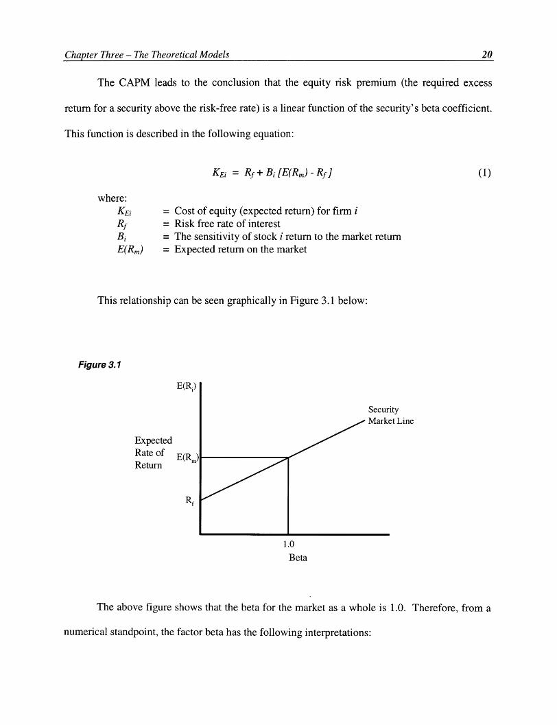
The CAPM leads to the conclusion that the equity risk premium (the required excess
return for a security above the risk-free rate) is a linear function of the security's beta coefficient.
This function is described in the following equation:
KEi = f + Bi [E(Rm) - Rf ]
where:KEi
Rf
BiE(Rm)
(1)
= Cost of equity (expected return) for firm i= Risk free rate of interest= The sensitivity of stock i return to the market return= Expected return on the market
This relationship can be seen graphically in Figure 3.1 below:
Figure 3.1
ExpectedRate ofReturn
ityt Line
1.0
Beta
The above figure shows that the beta for the market as a whole is 1.0. Therefore, from a
numerical standpoint, the factor beta has the following interpretations:

Chapter Three - The Theoretical Models 21
Beta > 1.0 The rates of return for the subject company tend to move in the samedirection and with greater magnitude than the market returns. Many hightech companies are examples of stocks with high betas.
Beta = 1.0 Movements in the rates of return for the subject tend to equal movementsin the rates of return for the market portfolio.
Beta < 1.0 When the market rates of return fluctuate, rates of return for the subjectcompany tend to also fluctuate, but to a lesser extent. Examples of lowbeta stocks include equity REITs and utilities.
Beta < 0 Rates of return for the subject company tend to move in the oppositedirection from changes in the market portfolio. Stocks with negative betasare very rare.
The CAPM, like most economic models, offers a theoretical framework for how
relationships should exist if certain assumptions hold. It is imperative that anyone who chooses
to employ the CAPM to predict returns or estimate the cost of equity understands the
assumptions underlying the model. The extent to which these assumptions are or are not met in a
real world application will have an impact on the usefulness of the CAPM for the valuation of
projects or investments. The main assumptions are listed below.
1. Investors are risk averse.
2. Rational investors seek to hold fully efficient (fully diversified) portfolios.
3. All investors have identical investment time horizons.
4. All investors have identical expectations about such variables as expected rates ofreturn and how capitalization rates are generated.
5. There exist no transaction costs.
6. There are no investment-related taxes
7. The borrowing and lending rates are equivalent.
8. The market has perfect divisibility and liquidity.
Chapter Three - The Theoretical Models 22
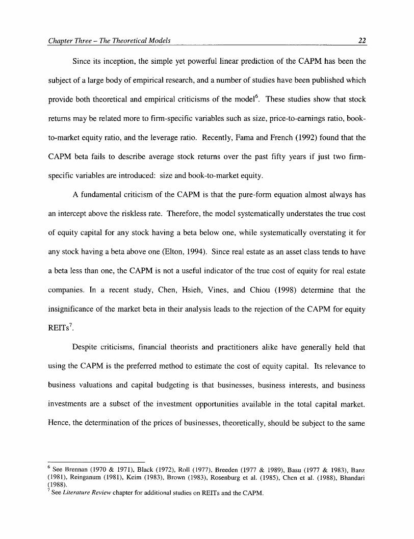
Since its inception, the simple yet powerful linear prediction of the CAPM has been the
subject of a large body of empirical research, and a number of studies have been published which
provide both theoretical and empirical criticisms of the model6. These studies show that stock
returns may be related more to firm-specific variables such as size, price-to-earnings ratio, book-
to-market equity ratio, and the leverage ratio. Recently, Fama and French (1992) found that the
CAPM beta fails to describe average stock returns over the past fifty years if just two firm-
specific variables are introduced: size and book-to-market equity.
A fundamental criticism of the CAPM is that the pure-form equation almost always has
an intercept above the riskless rate. Therefore, the model systematically understates the true cost
of equity capital for any stock having a beta below one, while systematically overstating it for
any stock having a beta above one (Elton, 1994). Since real estate as an asset class tends to have
a beta less than one, the CAPM is not a useful indicator of the true cost of equity for real estate
companies. In a recent study, Chen, Hsieh, Vines, and Chiou (1998) determine that the
insignificance of the market beta in their analysis leads to the rejection of the CAPM for equity
REITs 7.
Despite criticisms, financial theorists and practitioners alike have generally held that
using the CAPM is the preferred method to estimate the cost of equity capital. Its relevance to
business valuations and capital budgeting is that businesses, business interests, and business
investments are a subset of the investment opportunities available in the total capital market.
Hence, the determination of the prices of businesses, theoretically, should be subject to the same
6 See Brennan (1970 & 1971), Black (1972), Roll (1977), Breeden (1977 & 1989), Basu (1977 & 1983), Banz(1981), Reinganum (1981), Keim (1983), Brown (1983), Rosenburg et al. (1985), Chen et al. (1988), Bhandari(1988).7 See Literature Review chapter for additional studies on REITs and the CAPM.
Chapter Three - The Theoretical Models 23
economic forces and relationships that determine the prices of alternative investment assets
(Pratt, 1998).
THE FAMA-FRENCH MODEL
The Fama-French Model (FFM) is a multiple linear regression model developed by
Eugene Fama and Ken French in the early 1990s8. The FFM can be thought of as a multivariate
extension of the CAPM. The intuition is that there exist other factors that impact security prices
in addition to the movement of the market and the risk free rate. Fama and French propose that a
security's expected return depends on the sensitivity of its return to the market and the returns on
two portfolios meant to mimic these additional risk factors (Fama and French, 1997).
The additional mimicking portfolios are SMB (small minus big) and HML (high minus
low). SMB is the difference between the returns on a portfolio of small stocks and a portfolio of
big stocks, measured in terms of equity capitalization. The motivation for including SMB is to
capture the size premium present in historical common equity returns. Many empirical studies
performed since the CAPM was originally developed indicate that the realized total returns on
smaller companies have been substantially greater than predicted returns over a long period of
time9.
The other factor, HML, is the difference between the returns on a portfolio of high-book-
to-market-equity stocks and low-book-to-market-equity stocks. This "relative distress factor"
assumes that the earnings prospects of firms are associated with a risk factor in returns. Firms
that the market judges to have poor earnings prospects, signaled by low stock prices and high
8 See Fama, E.F., and K.R. French. "The Cross-Section of Expected Stock Returns." Journal of Finance (1992) 47,427-65, and "Common Risk Factors in the Returns on Stocks and Bonds." Journal of Financial Economics (1993)33, 3-56.9 See Banz (1981), Huberman and Kandel (1987), Berk (1995), etc.
Chapter Three - The Theoretical Models 23

Chapter Three - The Theoretical Models 24
ratios of book-to-market equity, have higher expected stock returns (hence, a higher cost of
equity capital) than firms with strong earnings prospects (Fama and French, 1992).
The expected return equation of the Fama-French Model is the following:
KE = Rf + Bil[E(Rm) - Rf ]+ Bi2[E(SMB)] + Bi3 [E(HML)] (2)
where:KEi = Cost of equity (expected return) for firm iRf = Risk free rate of interest (20-year T-Bond)Bil = The sensitivity of stock i return to the market returnE(Rm) = Expected return on the marketBi2 = The sensitivity of stock i to the return of a portfolio that mimics SMBE(SMB) = Expected return on a portfolio that mimics SMBBi3 = The sensitivity of stock i to the return of a portfolio that mimics HMLE(HML) = Expected return on a portfolio that mimics HML
Fama and French use six value-weighted portfolios formed on size and book-to-market
equity to construct the two specific risk factors in their model. Each year, all NYSE stocks on
the Center for Research in Securities Pricing (CRSP) tapes are ranked based upon price times
number of shares. The median NYSE size is then used to split NYSE, AMEX and NASDAQ
stocks into two groups, small (S) and big (B). In addition, they also divide the stocks into three
book-to-market equity groups based upon the bottom 30% (Low), middle 40% (Medium), and
top 30% (High) of the ranked values.
In their analysis, Fama and French define book common equity as the COMPUSTAT
book value of shareholders' equity plus balance-sheet deferred taxes and investment tax credit
minus the book value of preferred stock. The ratio of book-to-market equity is book common
equity for the fiscal year ending in calendar year t-l, divided by market equity at the end of
December of t-1 (Fama and French, 1993). It is interesting to note that only firms with ordinary
Chapter Three - The Theoretical Models 24

Chapter Three - The Theoretical Models 25
common equity (as classified by CRSP) are included in the tests. This means that ADRs, REITs,
and units of beneficial interest are excluded.
Fama and French then construct the six portfolios from the intersections of the two size
and three book-to-market equity groups. Monthly value-weighted returns on the six portfolios
are calculated from July of year t to June of t+l, and the portfolios are reformed in June of t+l.
The portfolio SMB is the difference each month between the simple average of the returns on
three small-stock portfolios (S/L, S/M, and S/H) and the simple average of the returns on the
three big stock portfolios (B/L, B/M, and B/H). Thus, SMB is the difference between the returns
on small-and big-stock portfolios with about the same weighted-average book-to-market equity.
This ensures the difference will be largely free of the influence of the book-to-market equity
factor, focusing instead on the different return behaviors of small and big stocks (Fama and
French, 1993).
The portfolio HML is defined in the same manner as SMB. HML is the difference each
month between the simple average of the returns on the two high book-to-market equity
portfolios (S/H and B/H) and the average of the returns on the two low book-to-market equity
portfolios (S/L and B/L). The two components of HML are returns on high and low book-to-
market equity portfolios with about the same weighted-average size. As a result, the difference
between the two returns should be largely free of the size factor in returns. Evidence of the
success of this simple procedure is reflected in the extremely low correlation between the two
monthly mimicking returns (Fama and French, 1993).
The results of Fama and French's initial study (1992) indicate that the CAPM beta does
not help explain the average returns on NYSE, AMEX, and NASDAQ stocks for the period 1963
through 1990. However, the two additional risk factors, SMB and HML, are statistically

Chapter Three - The Theoretical Models 26
significant predictors of returns over the same period. Similar results were obtained in
subsequent studies by Fama and French, as well as other researchers. The lack of support for the
CAPM is not surprising, as much of the financial research completed in the past 15 years arrives
at the same conclusion. However, the work of Fama and French is significant in that it shows
how two easily-measured variables can be used in practice to predict the cost of equity capital.
THE ARBITRAGE PRICING MODEL
The concept of Arbitrage Pricing Theory (APT) was introduced by Stephen Ross in
19761°. Similar to the FFM, APT can also be thought of as a multivariate extension of the
CAPM. In the APT model, the expected return (cost of equity) for an investment varies
according to that investment's sensitivity to a variety of risk factors, one of which may be a
CAPM-type market risk. The model itself does not specify what the risk factors are, but most
applications consider risk factors that are of a pervasive macroeconomic nature. Examples of
common risk factors used include unanticipated inflation, the unanticipated change in the term
structure, the unanticipated change in risk premium, and the unanticipated change in the growth
rate in industrial production.
In APT, as in the CAPM, there exist two sources of risk for any individual stock. First is
the risk associated with the macroeconomic factors which cannot be eliminated through
diversification, or systematic risk. Second is the risk arising from the possible events that are
unique to the specific company, or unsystematic risk. As with the CAPM, it is assumed that this
company-specific risk can be eliminated through holding stocks in large, well-diversified
10 See Ross, S.A. "The Arbitrage Theory of Capital Asset Pricing." Journal of Economic Theory (1976), 341-60.

Chapter Three - The Theoretical Models 27
portfolios. Therefore, the expected risk premium on a stock is affected only by factor or
macroeconomic risk (Brealey & Myers, 2000).
The econometric estimation of the Arbitrage Pricing Model (APM) with multiple risk
factors yields the following formula:
KE = Rf + Bil[E(K9)]+ Bi2 [E(K2 )] +... + Bin[E(Kn)] (3)
where:KE = Cost of equity (expected return) for firm iRf = Risk free rate of interest (20-year T-Bond)Bin = The sensitivity of stock i return to the return of a portfolio that mimics
KnE(K,) = Expected return on a portfolio that mimics factor K,
Notice that the APT formula makes two important statements (Brealy & Myers, 2000):
1. If a value of zero is plugged into each of the factor betas, the expected risk premiumis zero. A diversified portfolio that is constructed to have zero sensitivity to eachmacroeconomic factor is essentially risk-free, and therefore must be priced to offerthe risk-free rate of interest. If this did not hold, investors could make an arbitrageprofit.
2. A diversified portfolio that is constructed to have exposure to a factor will offer a riskpremium which will vary in direct proportion to the portfolio's sensitivity to thatfactor. For example, if portfolio A is twice as sensitive to a factor as portfolio B,portfolio A must offer twice the risk premium. If this did not hold, investors couldmake an arbitrage profit.
If the arbitrage pricing relationship as it is described above holds for all diversified
portfolios, then it must generally hold for individual stocks. Each stock must offer an expected
return commensurate with its contribution to portfolio risk. In the framework of APT, this
contribution depends on the sensitivity of the stock's return to the unexpected variations in the
specified macroeconomic factors.

Chapter Three - The Theoretical Models 28
Most academicians consider the Arbitrage Pricing Model (APM) richer in its
informational content and explanatory and predictive power than the CAPM. Empirical research
suggests that the multivariate APM explains expected rates of returns more effectively than the
univariate CAPM11. In fact, some researchers (Roll and Ross, 1980) propose APT as a testable
alternative, and perhaps natural successor to the CAPM.
1" See Chen (1983), Bower et al. (1984), Chen et al. (1986), and Berry et al. (1988).
Chapter Three - The Theoretical Models 28

Chapter Four - Literature Review 29
CHAPTER FOUR
Literature Review
REITs and the CAPM
Much research has been done comparing the returns of REITs to the returns of the overall
stock market. Although the results of these studies vary, essentially, the findings suggest that
REIT risk-adjusted returns have been superior to those of other stocks from the-mid 1960s
through the early 1980s, with a small number of aberrations. However, stock market portfolios
have dominated REIT returns since the mid-1980s.
One of the first studies to specifically compare the performance of equity REITs with that
of common stocks was by Smith and Shulman (1976). They tracked the quarterly returns of 16
equity REITs over eleven years from 1963 to 1974. These returns were contrasted against those
of the S&P composite index and a sample of closed-end funds by employing various measures
including comparing geometric mean returns, goodness of fit (R 2), and CAPM. The findings
revealed that equity REITs underperformed the broader market and fared about the same as the
closed-end funds. However, by reducing the holding period by one year (thus eliminating 1974,
a year in which the stock market experienced particularly high negative returns) equity REIT's
outperformed the S&P composite index.
In a subsequent study, Burns and Epley (1982) demonstrate that adding equity REITs to a
portfolio of common stocks results in a more efficient portfolio frontier. The data examines
quarterly returns, which include 35 REITs (10 equity REITs) from the first quarter of 1970
through the fourth quarter of 1979. The study explores various combinations of assets in order to
obtain the highest efficient portfolio frontier. Previous studies indicate that the correlation
Chapter Four - Literature Review 29

Chapter Four - Literature Review
coefficients between real estate and stocks is
assets produces a more efficient portfolio.
1970 through 1979, confirm that the outcome
surpasses single-asset portfolios at all points
return. Furthermore, this mixed asset portfolio
period.
30
s generally rather low. Hence, combining these
kccordingly, the results from the period between
of combining portfolios of both REITs and stocks
along the efficient frontier in terms of risk and
outperformed the S&P 500 index during the same
The findings of Walther (1986) and Kuhle (1987) reveal that REIT stocks outperformed
the S&P index during the 1977-1984 period, but underperformed the index from 1973-1976.
These results are also supported by research by Sagalyn (1990). This study examines the ex-post
real returns of REITs over the period from 1973 to 1987 and shows that equity REITS exhibited
less volatility with higher returns in comparison to the S&P 500 index.
A study by Howe and Shilling (1990) suggests that REITs have underperformed the
CRSP Equally-Weighted index from 1973 to 1987. In agreement with this, Gobel and Kim
(1989) examine the returns of 32 REITs over a four-year period from 1984-1987. They
compared their findings to the S&P 500 index, the Consumer Price Index, and Treasury bills.
Their results indicate that the sample of REITs underperformed the S&P 500 index over the
study period.
The findings from a research study performed by Martin and Cook (1991) determine
through using generalized stochastic dominance that stock portfolios generated slightly higher
risk-adjusted returns for the period between 1980-1990. Han and Liang (1995) studied eight
REIT portfolios during 1970-1993. Their results indicate that REIT stock performance was
slightly worse than the stock market portfolio. More recently, Chen and Peiser (1999) conclude

Chapter Four - Literature Review 31
that equity REITs underperformed both the S&P 500 index and the S&P Midcap 400 index over
the period 1993 through 1997.
REITs and the FFM
Up to this point, there have been no previous research projects which specifically use the
Fama-French model to estimate the returns of equity REITs. However, Fama and French
completed a study in 1997 which employs both the CAPM and the FFM to examine the cost of
equity for 48 industries, including Real Estate, for the period 1963 through 199412.
Unfortunately, the Real Estate industry used in the study did not include REITs. Fama and
French used four-digit SIC codes to form their industry groups, and because REITs have their
own SIC code separate from other real estate companies, they were included in a general Finance
industry. The results from the study are worth noting, however, as they provide additional
rationale for employing the FFM in our research.
Not surprisingly, the results from the 1997 study show large differences between the cost
of equity estimates obtained using CAPM and those using the FFM. For the five-year estimates,
the CAPM and FFM figures differ by more than 2% for 19 industries and by more than 3% for
15 industries (Fama and French, 1997). These differences are attributable to the SMB and HML
slopes in the three-factor regressions. Those industries with slopes close to zero consequently
produce results similar to the CAPM. Examples of industries where this occurs is Food,
Machinery, Electrical Equipment, Boxes, Building Materials, and Insurance.
Industries for which the CAPM and FFM produced significantly lower estimate for the
cost of equity include health industries (Health Services, Medical Equipment, and Drugs) and
12 See Fama, E.F., and K.R. French. "Industry Costs of Equity." Journal of Financial Economics (1997) 43, 153-93.

Chapter Four - Literature Review 32
high-tech industries (Computers, Chips, and Laboratory Equipment). This result is largely due to
strong negative risk loadings on the HML factor. The FFM identifies these as industries with
strong growth prospects over the sample period and rewards them with comparatively lower
costs of equity.
Conversely, many industries, including Real Estate, have cost of equity estimates using
the FFM that are at least 2% higher than those obtained using the CAPM. Specifically, Fama
and French estimated the industry cost of equity premium for Real Estate to be 5.99% using the
CAPM and 11.16% using the FFM . This dramatic difference is a function of the low beta of
real estate assets and the lack of significance of the CAPM in predicting returns for real estate
companies. Other industries where similar discrepancies also observed include Textiles,
Banking, Steel, and Autos. The FFM assigns high costs of equity for each of these industries
because their returns covary with the returns on small stocks (they have large positive slopes on
SMB) and because they behave like distressed stocks (they have large positive slopes on HML).
REITs and APT
There have been a number of research studies done in the past which attempt to link the
returns from real estate to market-level factors. Many studies indicate that certain variables such
as inflation and interest rates may be significant in predicting returns to real estate' 3 . In recent
years, researchers have used Arbitrage Pricing Theory to examine macroeconomic influences
using publicly traded REITs as the real estate proxy. The results from these studies vary widely
depending on the sample of REITs chosen and the time period examined. However, in most
13 See Hartzell et al. (1987), Fama and Schwert (1977), Rubens et al. (1989), Brueggeman et al. (1984), Ibbotson anSiegel (1984), and Miles and Mahoney (1997).

Chpe or-Ltrtr eiw3
cases, multifactor models are more effective at predicting REIT returns than the single-factor
CAPM.
Titman and Warga (1986)
Titman and Warga's is the first study to specifically examine the risk-adjusted
performance of REITs using both the CAPM and APT. Since it was generally viewed that the
returns from REITs, as well as real estate in general, were sensitive to inflation and interest rates,
Titman and Warga set out to examine whether the APM provided more accurate measures of
risk-adjusted returns.
The research sample consists of 16 equity and 20 mortgage REITs listed on the NYSE
and AMEX in 1973. The study examines the returns over two sample periods, January 1973
through December 1977, and January 1978 through December 1982. The single index, or
CAPM, models employ both the CRSP Value-Weighted index and Equally-Weighted index as
the market proxy. Two types of multiple-index models are also examined. The first includes a
portfolio of long-term government bonds along with the (Equally-Weighted or Value-Weighted)
market portfolio in a two-factor model. In addition, a model using five-factor portfolios formed
with maximum likelihood factor analysis is also examined. In theory, these portfolios are
designed to mimic changes in inflation, interest rates, and any other macroeconomic variables
that generate returns on capital assets.
The results of the study suggest that the single-index and multiple-index models can
provide very different estimates of the performance of REITs. In particular, the performance
measures are almost always higher for the models that included the Value-Weighted index as a
benchmark portfolio than they are for the models that include either the Equally-Weighted index
Chapter Four - Literature Review 33

Chapter Four - Literature Review 34
or the five-factor analysis portfolios. The five-factor model generates performance measures that
are substantially lower than those generated with the Value-Weighted market index. However,
since the single-factor model that employs the Equally-Weighted index as its benchmark
portfolio generates performance figures that are very similar to those produced by the five-factor
model, the above mentioned difference can not be attributed to the additional factors.
Titman and Warga conclude that neither the CAPM or APT-based techniques are
powerful enough to provide reliable evaluations of the investment performance of real estate
portfolios. The main reason for their result may be due to the research sample. The returns for
the chosen REITs over the period examined were extremely volatile. Therefore, even large
measures of abnormal performance were not statistically different from zero.
Chan, Hendershott, and Sanders (1990)
The purpose of this study is to examine the notion that real estate both provides
substantial risk-adjusted excess returns and serves as a hedge against inflation. Instead of using
traditional appraisal-based returns, Chan et al. analyze monthly returns of eighteen to twenty-
three equity REITs traded between 1973 to 1987. In their analysis, they use both the CAPM and
the APM to assess the relative riskiness of real estate returns.
The macroeconomic factors identified in this study are the same variables specified by
Chen, Roll, and Ross (1986). They include (1) industrial production growth, (2) the change in
expected inflation, (3) unexpected inflation, (4) the difference between the returns on low-grade
corporate bonds and long-term Treasury bonds, and (5) the difference in the returns between the
long-term Treasury bonds and the one-month T-Bill rate. REIT excess returns (returns over the
Chapter Four - Literature Review 35
risk-free rate) are regressed against excess returns of portfolios whose returns mimic the
individual prespecified factors to evaluate REIT risk-adjusted performance.
The study found that using a simple CAPM framework shows evidence of excess REIT
returns over the study period, most notably in the 1980s. However, this effect is eliminated
when using the multifactor arbitrage pricing approach. Furthermore, the APM shows that three
factors consistently drive both REIT and general stock market returns: changes in the risk and
term structures and unexpected inflation. Moreover, since unexpected inflation is shown to have
a negative impact, REITs are not a hedge against unexpected inflation, as is often believed to be
the case.
McCue and Kling (1994)
The purpose of this study is to identify and examine the relationship between the
macroeconomy and commercial real estate returns. More specifically, McCue and Kling set out
to determine the channels of influence followed by macroeconomic variables, the extent to which
the macroeconomic variables explain real estate returns, and how real estate returns react to
shocks in the macroeconomy.
Unlike previous research into real estate returns which use commingled real estate fund
data, McCue and Kling employ equity REIT data as the real estate data series. They examine
monthly returns of the NAREIT Composite index for the period from May 1974 through
December 1991. The four factors used as proxies for the macroeconomic variables include
prices (the Consumer Price Index), short-term nominal interest rates (the three-month Treasury
Bill rate), output (the Federal Reserve's Industrial Production Index), and investment (the
Chapter Four - Literature Review 35

Chapter Four - Literature Review 36
McGraw Hill Construction Contract Index). They utilize a vector autoregressive model for the
period examined, and estimate the coefficients by ordinary least squares.
McCue and Kling found that the macroeconomy explains nearly 60% of the variation in
equity REIT returns. Of the macroeconomic variables employed, nominal interest rates explain
the greatest percentage of variation, nearly 36% of the total. Conversely, the price, output, and
investment variables explain very little of the variation in returns. Shocks to nominal rates are
significantly negative, while shocks to investment and output are significantly positive. A shock
to prices results in a decline in REIT returns.
Chen, Hsieh, and Jordan (1997)
This aim of this study is to follow and expand the work of Titman and Warga (1986) and
Chan, Hendershott, and Sanders (1990) by utilizing Arbitrage Pricing Theory to explain real
estate returns. Chen et al. utilize two empirical implementations of APT: the factor loading
model and the macrovariable model. The study compares the ability of these two models to
explain the observed returns of equity REITs over three six-year periods, January 1974 -
December 1979, January 1980 - December 1985, and January 1986 - December 1991. The
sample includes 14, 12, and 27 equity REITs for each respective period.
The procedure utilized to determine the factor risk premiums is essentially identical to the
widely-used approach pioneered by Fama and MacBeth (1973). The factor premiums can be
interpreted as the predicted or fitted values from running a cross-sectional weighted least squares
regression of a prespecified industry portfolio on the factor loadings each month. For the
macrovariable model, the study uses the following variables: (1) the unanticipated inflation rate,
(2) the change in expected inflation, (3) the unanticipated change in term structure, (4) the

Chapter Four - Literature Review 37
unanticipated change in risk premium, and (5) a market index residual derived from regressing
the market index on the other four macrovariables.
The results of the study indicate that the five-factor macrovariable model is superior in
explaining equity REIT returns for two of the three time periods examined, January 1980 -
December 1985 and January 1986 - December 1991. In the remaining period (January 1974 -
December 1979) the hypothesis of equal performance could not be rejected. The macrovariable
model is also determined to be superior when the three periods are considered together.
Regarding the variables themselves, coefficients on the unanticipated inflation rate, the
unanticipated change in term structure, and the market residual are all significant at the 10%
level in the later two periods examined. None of the macrovariables are found to be significant
in the first period, the period for which both models have equal performance.
Chen, Hsieh, Vines, and Chiou (1998)
This study examines whether any of the common factors prevailing among ordinary
equities is useful in explaining the cross-sectional variation in equity REIT returns. The
difference between this and previous studies is most of the existing work investigating the
relative performance of REITs examines only time-series returns. Cross-sectional tests are
designed to explain differences in the returns across various assets in a specific time period.
Chen et al. employ four different pricing models to explain the returns of equity REITs.
The first is the traditional CAPM. The other three are multi-factor models differing in the
number and type of explanatory factors included. In the firm-specific variable model, the factors
are attributes unique to individual firms, namely firm size and the book-to-market equity ratio.
The macroeconomic variable model employs the same economic time-series variables used by

Chapter Four - Literature Review 38
Chen, Hsieh, and Jordan (1997). For the combined model, all the variables associated with the
other three models are combined together as factors.
The results of the study show that the regression coefficient associated with the market
beta is not significantly different from zero. Therefore, the data does not support the market
index as a relevant variable for explaining cross-sectional variation of equity REIT returns, and
CAPM is rejected. The study also shows that firm size is significantly priced among equity
REITs over time. The significance remains even when all of the other factors are present. The
book-to-market equity ratio is not significant in either of the two pricing models.
The results also indicate that the macroeconomic variables used are generally
insignificant in equity REIT pricing. The only exception is the unanticipated change in term
structure. The risk premium is negatively significant at the 5% level in the macroeconomic
variable model, but significance disappears in the combined model. In summary, Chen et al.
found that none of the macroeconomic variables are significant in explaining the cross-sectional
variation of equity REIT returns when the two firm-specific models are also included.

Chapter Five - The Research Models 39
CHAPTER FIVE
The Research Models
This study employs three asset-pricing models to estimate the cost of equity capital for
REITs. The first model is the traditional CAPM, where the total excess returns for each REIT in
the sample are regressed against the total excess returns of the broad market index14. The second
research model incorporates the two firm-specific factors developed by Fama and French, SMB
and HML. Again, ordinary least squares regression is used to estimate the required returns. In
the third model, two additional macroeconomic factors are included to represent the change in
expected inflation and the change in risk premium. Using factors that are of a pervasive
macroeconimic nature is in line with the Arbitrage Pricing Theory of Ross.
The goal of this study is to determine a model which produces results that are accurate
and consistent as to be used in practice. Therefore, our starting point for the research sample was
all 130 equity REITs in the four major property sectors: Office/Industrial, Retail, Residential
(Multifamily), and Diversified, as of December 31, 1999. Since the REIT industry has gone
through such dramatic changes in recent years, we imposed three additional criteria for the final
sample to insure accurate results. The first criterion was the existence of sixty consecutive
monthly returns from January 1995 through December 1999 on the Center for Research in
Security Prices (CRSP) tapes. This is to allow for the estimation of the betas in the regression
equations.
The second criterion was that each REIT have a Standard Industrial Classification (SIC)
code of 6798 for the entire sixty-month period. This is to ensure the company was organized as
14 Excess returns are monthly returns in excess of the one-month risk free rate.
39Chapter Five - The Research Models

Chapter Five - The Research Models 40
a REIT for the complete sample period. The unique requirements and limitations of the REIT
structure make these companies very different from other equities. Since the goal of this study is
to develop a model for equity REITs, we want to examine the historical returns of only those
companies organized as a REIT.
The third and final criterion is that the company has the same CRSP Permanent Number
for the entire sample period. The total research sample of 49 equity REITs is listed in Appendix
A. In order to determine a proxy for the overall REIT market, the total excess returns of the
NAREIT Value-Weighted indexes for all REITs and equity REITs are also examined.
THE RISK FACTORS
The most important element in estimating asset returns is the unexpected change in the
variables that affect asset prices. For instance, it is generally held that earnings expectations are
important in affecting the value of a company, and that earnings expectations are fully reflected
in the current share price. Thus, changes in expectations result in changes in the share price and
are directly reflected in returns. If an investor wants to predict the return for a company over a
certain period of time, the most important earnings variable is how earnings expectations change
- the actual earnings estimate or the error in the forecast becomes almost irrelevant.
Because only innovations or unanticipated changes in the variables are required, we use
realized total returns rather than stated yields or levels for our risk factor data'5 . There are
statistical tolls and methods that can be utilized to estimate the innovations from data such as
yields on Government Bonds and the level of the Consumer Price Index (CPI)16 . However, such
methods are not very efficient for use in practice, as continually updating the results becomes
15 Assuming efficient markets, actual returns are, by definition, innovations.

C F
cumbersome and time consuming. Using returns as opposed to yields enables the research
database to be updated easily using published data, and the factor premiums and coefficients to
be recalculated as needed.
The first two models used in this study, the CAPM and Fama-French Model, dictate
which risk factors are to be used to estimate stock returns. Conversely, the third model based
upon Arbitrage Pricing Theory does not specify which factors are to be employed. Therefore,
we draw upon previous research results for both general equities and REITs in defining the risk
factor variables for this model. As mentioned in a previous section, most applications of the
Arbitrage Pricing model consider risk factors that are of a pervasive macroeconomic nature. The
most common risk factors used are those first defined by Chen, Roll, and Ross (1986) and
include changes in expected inflation, changes in unexpected inflation, the unanticipated change
in the term structure, the unanticipated change in risk premium, and the unanticipated change in
the growth rate in industrial production.
Based upon recent studies dealing specifically with real estate, notably Chan,
Hendershott, and Sanders (1990) the unanticipated change in industrial production is not
included in our model. Despite the fact that their study also found no significant role in the
change in expected inflation for equity REIT returns, the variable is retained in our model due to
the amount of empirical findings related to the impact of inflation on real estate. Furthermore,
since it has been shown that changes in expected inflation are highly correlated with changes in
unexpected inflation, we do not add an additional factor for this risk.
We also do not include an additional variable for the change in term structure. This is
due to the fact that our variable for the change in expected inflation is the one-year Treasury
16 See Fama and MacBeth (1973).
Chater Five - The Research Models 41

Chapter Five - The Research Models 42
Bond less the one-month Treasury Bill. Since, theoretically, the change in term structure can be
measured by the difference between any two points on the yield curve, this factor captures some
of this effect. Moreover, the high correlation between the change in term structure factor and the
change in expected inflation factor would cause erroneous results.
Of the common factors used in Arbitrage Pricing Models, we employ only two: the
change in expected inflation and the change in the risk premium (which we label as Confidence
Risk). Because of the overwhelming significance of the two Fama-French factors and their
universal applicability, they are retained for our combined model. Furthermore, we also use the
market premium from the CAPM in order to assess its significance in the presence of additional
factors.
Each of the risk factors used in this paper is identified and discussed below.
1. Market Risk (MKP)
In the CAPM model, the MKP is the only risk factor employed. This follows from
Capital Market Theory which states that all systematic risk is represented by the single market
beta coefficient.
In the multifactor models, including the MKP factor makes the CAPM a special case. In
the FFM and APM, the MKP represents that part of the total market return that is not explained
by the other variables and an intercept term. Therefore, if the risk exposure to all of the other
factors is exactly zero, than the MKP is proportional to the total market return. Under these
extremely unlikely conditions, a stock's exposure to MKP would be exactly equal to its CAPM
beta. By retaining the MKP, the FFM and APM can be viewed as extensions or generalizations
of the CAPM.

Chapter Five - The Research Models 43
2. Size Factor (SMB)
The Size Factor is used to capture the size premium that exists in common equity returns.
This factor was constructed by Eugene Fama and Ken French and represents the difference
between the returns on a portfolio of small stocks and a portfolio of big stocks, measured in
terms of equity capitalization. See Chapter Three for a complete description of the derivation of
SMB.
We expect SMB to have a significant impact on the cost of equity for REITs. Correcting
for the size disparity is important for this industry, as the average REIT is much smaller than the
average company listed on the NYSE. Furthermore, Colwell and Park (1990) and McIntosh,
Liang, and Tompkins (1991) find the small firm effect exists within the REIT industry.
3. Relative Distress Factor (HML)
The Relative Distress Factor (HML) is the other Fama-French factor employed in this
study. HML is used to account for the return premium that exists for companies with relatively
high book-to-market-equity ratios. The factor is measured as the difference between the total
returns on a portfolio of high-book-to-market-equity stocks and low-book-to-market-equity
stocks.
The Relative Distress Factor assumes that the earnings prospects of firms are associated
with a risk factor in returns. Firms that have high book-to-market-equity ratios (a low stock
price relative to book value) tend to have low earnings on assets, and the low earnings persist for
at least five years before and five years after the ratio is measured. Conversely, firms with low
book-to-market-equity ratios (a high stock price relative to book value) tend to have persistently
high earnings (Fama and French, 1993). Consequently, firms that the market judges to have poor

44
earnings prospects, have higher expected stock returns (a higher cost of equity capital) than firms
with strong earnings prospects.
Research by Fama and French indicate that, despite the fact that the size effect has
attracted more attention, the book-to-market equity ratio has a consistently stronger role in
predicting returns (Fama and French, 1992). Given that HML is significant in measuring the
returns for other equities, we expect it to be an important factor in measuring the cost of equity
for REITs.
4. Change in Expected Inflation (EXI)
The Change in Expected Inflation represents the unanticipated changes in investors'
outlook on inflation. There are many options that can be used to proxy inflation expectations.
Several studies use the forecast for the Consumer Price Index or various estimates from
professional surveys. However, as mentioned previously, determining the innovations from a
time-series of yields is not efficient for a model designed to be used in practice. Therefore, we
use the excess return on the one-year U.S. Treasury Bond to proxy the Change in Expected
Inflation. Existing interest rate literature indicates that the movements in short-term U.S.
Government securities are primarily due to changes in inflation expectations'7. Hence, the one-
year Bond can be thought of as representing investors' expectations for inflation for the next
year.
Most stocks have negative exposures to changes in expected inflation. Thus, a positive
inflation surprise causes a negative contribution to return, whereas a negative inflation surprise (a
17 See Fama (1975).
Chapter Five - The Research Models

Chapter Five - The Research Models 45
deflation shock) contributes positively toward returns (Burmeister, 1994)18. Alternatively,
companies that have large asset holdings, such as real estate, may actually benefit from increased
inflation. Several research studies indicate that unsecuritized real estate provides an effective
hedge against the expected and unexpected components of inflation19. Studies which examine
the relationship between REITs and inflation have not been as conclusive, however. Some
studies show that REITs and inflation are unrelated, while others indicate that REITs provide a
hedge against the temporary or permanent components of certain inflation measures20.
5. Confidence Risk (CON)
Confidence Risk is the unanticipated changes in investors' willingness to undertake
relatively risky investments. CON is measured as the difference between the rate of return on
relatively risky (Baa) and relatively safe (Aaa) corporate bonds. In any month when the return
on Baa-rated bonds exceeds the return on Aaa-rated bonds by more than the long-run average,
this measure of Confidence Risk is positive. The intuition is that a positive return difference
reflects investor confidence because the required yield on relatively risky bonds has fallen with
respect to relatively safe bonds. Most equities have a positive exposure to CON, and small
stocks generally have greater exposure than large stocks (Burmeister, 1994).
18 In this study, EXI is measured in terms of returns, not yields. Therefore, the relationship to unanticipated changesin inflation is the same as stated, but the sign on the coefficients is the opposite.19 See Chapter Four.
20 For unrelated, see Murphy and Kleiman (1989), Chen et al. (1990), Park et al. (1990), and Yabaccio et al. (1995).For related, see Gyourko and Linneman (1988), Chen and Tzang (1988), and Chatrath and Liang (1998).

Chapter Five - The Research Models 46
Table 5.1 provides a summary of the risk factors and their derivation.
Table 5.1Glossary and
Symbol VariablePanel A: Basic Data Series and Source
Market t Stock market index
1MoTB t Treasury-bill rate
SMB t FF size factor
HML t FF distress factor
1 YrTB t Treasury-bond rate
Aaa t Aaa-rated industrial bor
Baa t Baa-rated industrial bor
Measurement of Risk Factor Variables
Data Source or Measurement
Total return on value-weighted portfolio of all NYSE, AMEX, andNASDAQ stocks (CRSP)
U.S. Treasury Bill total returns (Ibbotson Associates, 2000)
Total average return on three small portfolios minus three bigportfolios (Ken French)
Total average return on two value portfolios minus two growthportfolios (Ken French)
U.S. Treasury Bond total returns (CRSP)
Total return on Lehman Bros. Investment Grade Aaa Long Index(Datastream)
Total return on Lehman Bros. Investment Grade Baa Long Index(Datastream)
Panel B: Derived Risk Factors
MKP t Market Risk Market t - 1MoTB t
SMB t Size Factor 1/3 (small value + small neutral +small growth) - 1/3(big value +big neutral + big growth)
HML t Relative Distress Factor 1/2 (small value + big value) - 1/2 (small growth + big growth)
EXI t Change in Expected Inflation 1YrTB t - 1MoTB t
CON t Confidence Risk Baa t -Aaa t
Factor Risk Premiums
In order to determine the premiums required for each of the various risk factors, we first
compiled the total monthly returns for each variable over the 27-year period from January 1973
through December 199921. Next, we perform the necessary operations to derive the returns for
each of the risk factors. For example, the total returns for each month for the 30-day Treasury
.
nd
nd

Chapter Five - The Research Models 47
Bill is subtracted from those of the CRSP Value-Weighted Index to determine the monthly
Market Risk (MKP) returns. After the 324 monthly returns for each of the derived factors are
compiled, the simple arithmetic mean is computed 22. The mean monthly premium was then
annualized to ascertain the factor risk premium. Table 5.2 below lists each factor and associated
annual risk premium.
Table 5.2
Factor Risk Premiums%, for the period 1/73 - 12/99
Avg. Monthly Standard AnnualReturn Deviation Premium
Market Risk - MKP 0.61 4.61 7.27Size Factor- SMB 0.12 2.87 1.46Relative Distress Factor - HML 0.30 2.93 3.56Change in Expected Inflation - EXI 0.11 0.58 1.28Confidence Risk - CON 0.09 1.05 1.04
THE CAPITAL ASSET PRICING MODEL
Estimating the cost of equity capital for each REIT using the CAPM is relatively
straightforward. As mentioned previously, the required rate of return is composed of only two
factors, the risk-free rate and the company's relationship to the market's general risk premium.
Regarding the risk-free rate, the general consensus of practitioners is to use the 20-year U.S.
Treasury yield to maturity as of the effective day of valuation for the following reasons (Pratt,
1998):
21 The sample period was determined by data availability. Specifically, the data series for the Lehman BrothersInvestment-Grade Corporate Bond Index begins in January 1973.22 Following common practice, the arithmetic mean is used as opposed to the geometric mean [see Pratt (1998),Ibbotson (2000), and Brealey and Myers (2000)].
Chapter Five - The Research Models 48
1. It most closely matches the often-assumed perpetual lifetimehorizon of an equity investment.
2. The longest-term yields to maturity fluctuate considerably less thanshort-term rates and thus are less likely to introduce unwarrantedshort-term distortions into the actual cost of capital.
3. People are generally willing to recognize and accept the fact thatthe maturity risk is impounded into this base, or otherwise risk-free, rate.
4. For compiling historical data, 20 years was the longest U.S.Treasury obligation issued during the early part of the twentiethcentury.
Many analysts use a 30-year yield, but as a practical matter it usually is not greatly
different than the 20-year yield.
The second factor in the CAPM is the Market Risk Premium (MKP). Since the expected
total return on equities is much more risky than the interest and maturity payments on U.S.
Treasury obligations, investors require a comparatively higher return for investing in equities.
This excess return is known as the Market Risk Premium.
In practice, a common method for estimating the expected MKP is to use historical data.
It is important to note, however, that doing so assumes the amount of excess return investors
expect for the future time horizon is approximately equal to the excess returns that have actually
been achieved in the historical period for which the premium was computed. As shown in Table
5.2, the average market premium from 1973 to 1999 was 7.27%23.
The specific application of Equation (1) used for estimating the cost of equity capital in
this study is identified below:
KEi = Rf + Bi [E(MKP)] (la)
23 Ibbotson Associates reports the 72-year (1926-1997) historical premium as 7.5%.

Chapter Five - The Research Models 49
where:KEi = Cost of equity (expected total return) for REIT iRf = Risk free rate of interest (20-year T-Bond)Bil = The sensitivity of REIT i excess return to the excess market returnE(MKP) = Expected excess return on the market
Given the calculated market risk premium of 7.27% and the 20-year Treasury yield of
6.69% as of December 31, 1999, the estimated cost of equity for the average U.S. public
company (B = 1.0) is about 14%:
KE = 6.69+ 1.0 (7.27)= 13.96%
In Equation (la), Bi is the sensitivity of REIT i to the return on the CRSP Value-
Weighted Index. We estimate Bi for each REIT in the research sample by examining the
historical relationship between the REIT and the broad market for the 60-month period January
1995 through December 1999. The value is estimated by fitting the time-series regression in the
form:
Ri, - Rft = ai + Bi(MKP) + eit (5)
where:Ri, - Rft = Total return for REIT i in month t less the total return on the one-month
T-Bill in month tai = Intercept for REIT iMKP = Total excess return on the CRSP Index in month tBi = The sensitivity of REIT i excess return to the excess market returneit = Residual for REIT i in period t, assumed to have a mean of zero
Results
The results from the CAPM regression equation and the estimated cost of equity for each
REIT in the research sample, the entire research sample (average returns), and the two NAREIT
indexes are displayed in Table 5.3.
Chapter Five - The Research Models 49

Chapter Five - The Research Models 50
Table 5.3 - CAPM Model Regression ResultsRi - Rf = ai + B (MKP) + ei
Coefficients t- statisticsREIT a B t(a) t(B) R2 KENAREIT Index
All REITs -0.399 0.399 -0.913 4.030 0.22 9.59Equity REITs -0.334 0.376 -0.772 3.841 0.20 9.42
Office / IndustrialDuke-Weeks Realty Corporation -0.007 0.471 -0.010 3.014 0.14 10.12Spieker Properties, Inc. 1.127 0.052 1.507 0.308 0.00 7.07Liberty Property Trust -0.093 0.506 -0.141 3.381 0.16 10.37Mack-Cali Realty Corporation 0.271 0.517 0.391 3.294 0.16 10.45Highwoods Properties, Inc. -0.412 0.544 -0.542 3.163 0.15 10.64CarrAmerica Realty Corporation -0.261 0.544 -0.368 3.388 0.17 10.64HRPT Properties Trust -0.715 0.441 -1.078 2.939 0.13 9.90First Industrial Realty Trust, Inc. -0.034 0.623 -0.044 3.585 0.18 11.22Koger Equity, Inc. 0.833 0.437 0.818 1.897 0.06 9.87Pacific Gulf Properties, Inc. 0.190 0.470 0.277 3.018 0.14 10.10Keystone Property Trust 1.241 0.482 0.994 1.706 0.05 10.20Average 0.195 0.463 0.375 3.934 0.21 10.05
RetailKimco Realty Corporation 0.060 0.368 0.088 2.380 0.09 9.36General Growth Properties, Inc. 0.486 0.065 0.678 0.403 0.00 7.17New Plan Excel Realty Trust, Inc. 0.455 0.304 0.538 1.588 0.04 8.90Regency Realty Corporation 0.269 0.235 0.394 1.521 0.04 8.40Developers Diversified Realty Corporation -0.355 0.211 -0.546 1.437 0.03 8.23Macerich Company, The -0.358 0.397 -0.513 2.518 0.10 9.58Taubman Centers, Inc. 0.120 0.223 0.196 1.618 0.04 8.31Realty Income Corporation 0.330 0.237 0.474 1.502 0.04 8.41CBL & Associates Properties, Inc. 0.168 0.075 0.288 0.565 0.01 7.23Chelsea GCA Realty, Inc. -0.005 0.331 -0.006 1.758 0.05 9.10Mills Corporation, The -0.179 0.426 -0.184 1.936 0.06 9.79Glimcher Realty Trust -1.033 0.478 -1.226 2.509 0.10 10.17Commercial Net Lease Realty, Inc. -0.752 0.513 -1.090 3.284 0.16 10.42JP Realty, Inc. -0.601 0.307 -0.831 1.875 0.06 8.92Saul Centers, Inc. 0.045 0.246 0.065 1.568 0.04 8.48Crown American Realty Trust -1.399 0.401 -1.331 1.683 0.05 9.61Mid-Atlantic Realty Trust 0.319 0.312 0.401 1.736 0.05 8.96Acadia Realty Trust -1.855 0.348 -2.350 1.946 0.06 9.22Kranzco Realty Trust -1.142 0.409 -1.238 1.956 0.06 9.66Ramco-Gershenson Properties Trust -0.553 0.266 -0.940 1.993 0.06 8.62Malan Realty Investors, Inc. 0.550 0.054 0.725 0.314 0.00 7.08Average -0.259 0.296 -0.578 2.918 0. 13 8.84
Residential (Multifamily)Equity Residential Properties Trust 0.061 0.476 0.089 3.063 0.14 10.15Apartment Investment & Mgmt. Co. 1.232 0.308 1.678 1.850 0.06 8.93Camden Property Trust -0.077 0.359 -0.107 2.216 0.08 9.30BRE Properties, Inc. 0.680 0.108 0.982 0.686 0.01 7.47Gables Residential Trust 0.222 0.187 0.374 1.388 0.03 8.05Essex Property Trust, Inc. 1.075 0.330 1.515 2.053 0.07 9.09Summit Properties Inc. -0.117 0.222 -0.187 1.565 0.04 8.30Mid-America Apartment Communities, Inc. -0.532 0.387 -0.846 2.719 0.11 9.51Town and Country Trust, The 0.127 0.501 0.208 3.618 0.18 10.33Associated Estates Realty Corporation -1.536 0.372 -1.745 1.864 0.06 9.39Average 0.114 0.325 0.234 2.962 0.13 9.05
DiversifiedVornado Realty Trust 0.814 0.255 0.898 1.241 0.03 8.54Crescent Real Estate Equities, Inc. -0.393 0.796 -0.420 3.754 0.20 12.48Washington Real Estate Investment Trust -0.377 0.270 -0.725 2.297 0.08 8.66Colonial Properties Trust -0.299 0.414 -0.518 3.168 0.15 9.70Pennsylvania Real Estate Investment Trust -0.146 0.107 -0.207 0.668 0.01 7.47Transcontinental Realty Investors, Inc. -0.110 0.439 -0.104 1.832 0.05 9.88Boddie-Noell Properties, Inc. -0.325 0.114 -0.456 0.704 0.01 7.52Average -0.119 0.342 -0.271 3.431 0.17 9.18
TOTAL SAMPLE AVERAGE -0.061 0.346 -0.143 3.566 0~~O. 17 .18 92
TOTAL SAMPLE AVERAGE -0.061 0.346 -0.143 3.566 0.18 9.20

Chapter Five - The Research Models 51
As expected, the CAPM systematically understates the cost of equity capital for equity
REITs. The average cost of equity estimate for the research sample is 9.20%, with a standard
error (s.e.) of 3.07%. Using standard convention of plus or minus two standard errors from the
mean, the average cost of equity falls between 3.06% and 15.34%. In addition, the MKP factor
is only significant at the 5% level in less than 45% of the individual time-series regressions. It is
significant at the 10% level in 65% of the regressions.
The range for the total sample is 7.07% (Spieker Properties) to 12.48% (Crescent Real
Estate Equities). The estimate for many of the REITs is less than their respective unsecured
borrowing costs. The highest average property sector estimate is for the Office/Industrial sector
at 10.05% (s.e. = 3.7%). The Retail sector has the lowest estimate at 8.84% (s.e. = 3.2%). Since
the REITs are organized in terms of equity market capitalization, we can examine the
relationship between the cost of equity estimate and company size within each property sector.
In the CAPM results, there is little evidence to support the claim that larger companies enjoy a
lower cost of equity capital.
The best and most widely used measure of the explanatory ability of a linear regression
model is the coefficient of determination, denoted by R 2. The R 2 for the CAPM is 0.18,
indicating the model only explains 18% of the variation in the average returns for the research
sample. The range of R 2 's for the individual REITs in the research sample is 0.00 (three REITs)
to 0.20 (Crescent Real Estate Equities). The extremely low coefficients of determination
indicate the lack of predictive ability of the CAPM, and suggest the model is not particularly
useful for estimating the cost of equity for REITs.

Chapter Five - The Research Models 52
THE FAMA-FRENCH MODEL
The method for estimating the cost of equity capital using the Fama-French Model (FFM)
is identified as the following application of Equation (2):
KE = Rf + Bil[E(MKP )]+ Bi2[E(SMB)] + Bi3[E(HML)] (2a)
where:KEi
RfBilE(MKP)Bi2
E(SMB)Bi3
E(HML)
= Cost of equity (expected return) for REIT i= Risk free rate of interest (20-year T-Bond)= The sensitivity of REIT i excess return to the excess market return= Expected excess return on the market= The sensitivity of REIT i excess return to the return of a portfolio that
mimics SMB= Expected return on a portfolio that mimics SMB= The sensitivity of REIT i excess return to the return of a portfolio that
mimics HML= Expected return on a portfolio that mimics HML
The factor sensitivities (B's) are calculated the same way as in the CAPM model. The
historical total monthly excess returns for each REIT are regressed against the total excess
returns for the market-portfolio, the SMB portfolio, and the HML portfolio for the 60-month
period January 1995 through December 1999. The values are estimated by fitting the following
time-series regression equation:
Rit - Rft = ai + Bil(MKP) + Bi2(SMB) + Bi3(HML) + eit (7)

Chapter Five - The Research Models
= Total return for REIT i in month t less the total return on the one-monthT-Bill in month t
= Intercept for REIT i= Total excess return on the CRSP Index in month t= The sensitivity of REIT i excess return to the excess market return= Total return the SMB portfolio= The sensitivity of REIT i excess return to the SMB portfolio return= Total return on the HML portfolio= The sensitivity of REIT i excess return to the HML portfolio return= Residual for REIT i in period t, assumed to have a mean of zero
Results
The results from the Fama-French regression equation and the estimated cost of equity
for each REIT in the research sample, the entire research sample (average returns), and the two
NAREIT indexes are displayed in Table 5.4.
where:Ri - gf,
aiMKPBilSMBBi2HMLBi3
eit
53
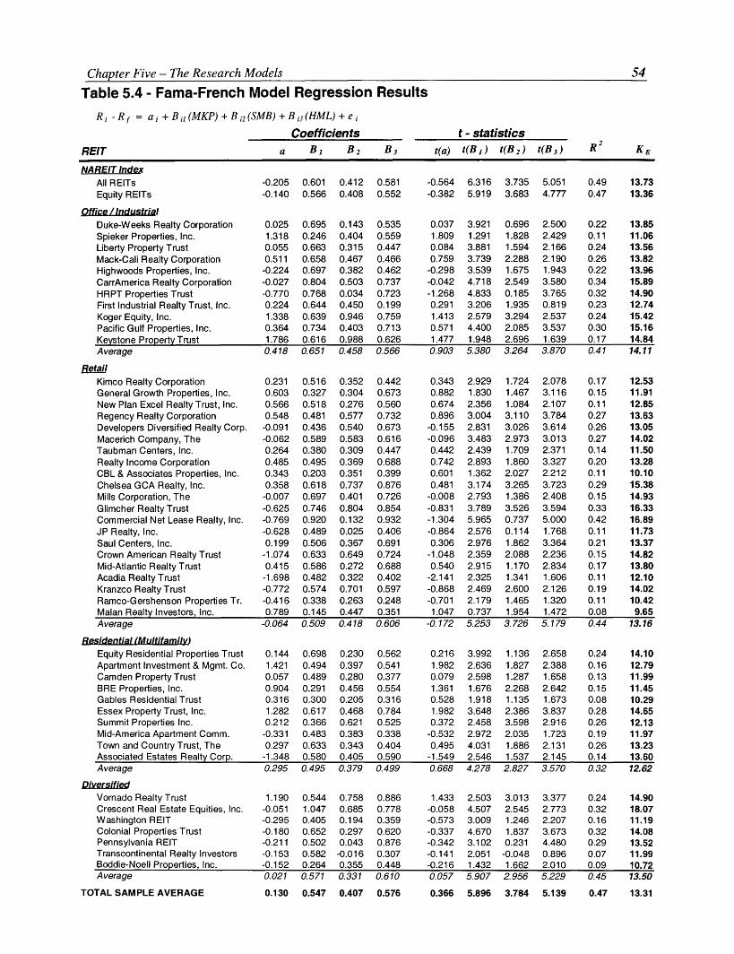
Chapter Five - The Research Models 54
Table 5.4 - Fama-French Model Regression ResultsRi -Rf = ai +Bil(MKP) + Bi 2 (SMB) +Bi 3(HML)+ei
Coefficients t- statisticsREIT a B1 B 2 B3 t(a) t(B 1) t(B 2) t(B ) R2 K
NAREIT IndexAll REITs -0.205 0.601 0.412 0.581 -0.564 6.316 3.735 5.051 0.49 13.73Equity REITs -0.140 0.566 0.408 0.552 -0.382 5.919 3.683 4.777 0.47 13.36
Office /ndustrialDuke-Weeks Realty Corporation 0.025 0.695 0.143 0.535 0.037 3.921 0.696 2.500 0.22 13.85Spieker Properties, Inc. 1.318 0.246 0.404 0.559 1.809 1.291 1.828 2.429 0.11 11.06Liberty Property Trust 0.055 0.663 0.315 0.447 0.084 3.881 1.594 2.166 0.24 13.56Mack-Cali Realty Corporation 0.511 0.658 0.467 0.466 0.759 3.739 2.288 2.190 0.26 13.82Highwoods Properties, Inc. -0.224 0.697 0.382 0.462 -0.298 3.539 1.675 1.943 0.22 13.96CarrAmerica Realty Corporation -0.027 0.804 0.503 0.737 -0.042 4.718 2.549 3.580 0.34 15.89HRPT Properties Trust -0.770 0.768 0.034 0.723 -1.268 4.833 0.185 3.765 0.32 14.90First Industrial Realty Trust, Inc. 0.224 0.644 0.450 0.199 0.291 3.206 1.935 0.819 0.23 12.74Koger Equity, Inc. 1.338 0.639 0.946 0.759 1.413 2.579 3.294 2.537 0.24 15.42Pacific Gulf Properties, Inc. 0.364 0.734 0.403 0.713 0.571 4.400 2.085 3.537 0.30 15.16Keystone Property Trust 1.786 0.616 0.988 0.626 1.477 1.948 2.696 1.639 0.17 14.84Average 0.418 0.651 0.458 0.566 0.903 5.380 3.264 3.870 0.41 14.11
RetailKimco Realty Corporation 0.231 0.516 0.352 0.442 0.343 2.929 1.724 2.078 0.17 12.53General Growth Properties, Inc. 0.603 0.327 0.304 0.673 0.882 1.830 1.467 3.116 0.15 11.91New Plan Excel Realty Trust, Inc. 0.566 0.518 0.276 0.560 0.674 2.356 1.084 2.107 0.11 12.85Regency Realty Corporation 0.548 0.481 0.577 0.732 0.896 3.004 3.110 3.784 0.27 13.63Developers Diversified Realty Corp. -0.091 0.436 0.540 0.673 -0.155 2.831 3.026 3.614 0.26 13.05Macerich Company, The -0.062 0.589 0.583 0.616 -0.096 3.483 2.973 3.013 0.27 14.02Taubman Centers, Inc. 0.264 0.380 0.309 0.447 0.442 2.439 1.709 2.371 0.14 11.50Realty Income Corporation 0.485 0.495 0.369 0.688 0.742 2.893 1.860 3.327 0.20 13.28CBL & Associates Properties, Inc. 0.343 0.203 0.351 0.399 0.601 1.362 2.027 2.212 0.11 10.10Chelsea GCA Realty, Inc. 0.358 0.618 0.737 0.876 0.481 3.174 3.265 3.723 0.29 15.38Mills Corporation, The -0.007 0.697 0.401 0.726 -0.008 2.793 1.386 2.408 0.15 14.93Glimcher Realty Trust -0.625 0.746 0.804 0.854 -0.831 3.789 3.526 3.594 0.33 16.33Commercial Net Lease Realty, Inc. -0.769 0.920 0.132 0.932 -1.304 5.965 0.737 5.000 0.42 16.89JP Realty, Inc. -0.628 0.489 0.025 0.406 -0.864 2.576 0.114 1.768 0.11 11.73Saul Centers, Inc. 0.199 0.506 0.367 0.691 0.306 2.976 1.862 3.364 0.21 13.37Crown American Realty Trust -1.074 0.633 0.649 0.724 -1.048 2.359 2.088 2.236 0.15 14.82Mid-Atlantic Realty Trust 0.415 0.586 0.272 0.688 0.540 2.915 1.170 2.834 0.17 13.80Acadia Realty Trust -1.698 0.482 0.322 0.402 -2.141 2.325 1.341 1.606 0.11 12.10Kranzco Realty Trust -0.772 0.574 0.701 0.597 -0.868 2.469 2.600 2.126 0.19 14.02Ramco-Gershenson Properties Tr. -0.416 0.338 0.263 0.248 -0.701 2.179 1.465 1.320 0.11 10.42Malan Realty Investors, Inc. 0.789 0.145 0.447 0.351 1.047 0.737 1.954 1.472 0.08 9.65Average -0.064 0.509 0.418 0.606 -0.172 5.253 3.726 5.179 0.44 13.16
Residential (Multifamily)Equity Residential Properties Trust 0.144 0.698 0.230 0.562 0.216 3.992 1.136 2.658 0.24 14.10Apartment Investment & Mgmt. Co. 1.421 0.494 0.397 0.541 1.982 2.636 1.827 2.388 0.16 12.79Camden Property Trust 0.057 0.489 0.280 0.377 0.079 2.598 1.287 1.658 0.13 11.99BRE Properties, Inc. 0.904 0.291 0.456 0.554 1.361 1.676 2.268 2.642 0.15 11.45Gables Residential Trust 0.316 0.300 0.205 0.316 0.528 1.918 1.135 1.673 0.08 10.29Essex Property Trust, Inc. 1.282 0.617 0.468 0.784 1.982 3.648 2.386 3.837 0.28 14.65Summit Properties Inc. 0.212 0.366 0.621 0.525 0.372 2.458 3.598 2.916 0.26 12.13Mid-America Apartment Comm. -0.331 0.483 0.383 0.338 -0.532 2.972 2.035 1.723 0.19 11.97Town and Country Trust, The 0.297 0.633 0.343 0.404 0.495 4.031 1.886 2.131 0.26 13.23Associated Estates Realty Corp. -1.348 0.580 0.405 0.590 -1.549 2.546 1.537 2.145 0.14 13.60Average 0.295 0.495 0.379 0.499 0.668 4.278 2.827 3.570 0.32 12.62
DiversifiedVornado Realty Trust 1.190 0.544 0.758 0.886 1.433 2.503 3.013 3.377 0.24 14.90Crescent Real Estate Equities, Inc. -0.051 1.047 0.685 0.778 -0.058 4.507 2.545 2.773 0.32 18.07Washington REIT -0.295 0.405 0.194 0.359 -0.573 3.009 1.246 2.207 0.16 11.19Colonial Properties Trust -0.180 0.652 0.297 0.620 -0.337 4.670 1.837 3.673 0.32 14.08Pennsylvania REIT -0.211 0.502 0.043 0.876 -0.342 3.102 0.231 4.480 0.29 13.52Transcontinental Realty Investors -0.153 0.582 -0.016 0.307 -0.141 2.051 -0.048 0.896 0.07 11.99Boddie-Noell Properties, Inc. -0.152 0.264 0.355 0.448 -0.216 1.432 1.662 2.010 0.09 10.72Average 0.021 0.571 0.331 0.610 0.057 5.907 2.956 5.229 0.45 13.50
TOTAL SAMPLE AVERAGE 0.130 0.547 0.407 0.576 0.366 5.896 3.784 5.139 0.47 13.31

Chapter Five - The Research Models 55
The predictive ability of the regression model is greatly improved with the addition of the
two Fama-French factors. The SMB factor is significant at the 5% level in nearly 40% of the
individual REIT regressions, and significant at the 10% level in 63% of the regressions. The
HML factor is significant at the 5% level in nearly 80% of the regressions, and significant at the
1% level nearly half of the time. At the 10% level HML is significant in nearly 90% of the
regressions. With the addition of the two Fama-French factors, the MKP factor also gains
significance. The MKP factor is significant at the 5% level in 84% of the regressions, and
significant at the 10% level in all but four of them. The resulting coefficient of determination is
0.47 for the total research sample. This indicates that the FFM explains approximately half of
the variation in REIT returns over the 60-month sample period, nearly a 30% improvement over
the CAPM.
The FFM cost of equity estimate using the average returns for the total research sample is
13.31%. In order to calculate the estimate error, the following equation is used:
s.e.(KE) = [var(MKp) x MKP2 + var(sMB) x SMB2 + var(HML) X HML2 + 2COV(MKP,SMB) x MKP (8)x SMB + 2COV(MB,HML) x SMB x HML + 2COV(MKP,HML) x MKP x HML] %
where:s.e.(KE) = The standard error of the cost of equity estimatevar(MKP) = Variance in the monthly returns for MKP, 1/95 - 12/99MKP = The historical MKP risk factor premiumvar(sMB) = Variance in the monthly returns for SMB, 1/95 - 12/99SMB = The historical SMB risk factor premiumvar(HML) = Variance in the monthly returns for HML, 1/95 - 12/99HML = The historical HML risk factor premiumCOV(MKP,SMB) = Covariance in monthly returns for MKP and SMB, 1/95-12/99COV(SMB,HML) = Covariance in monthly returns for SMB and HML, 1/95-12/99COV(MKP,HML) = Covariance in monthly returns for MKP and HML, 1/95-12/99

Chapter Five - The Research Models 56
The result of Equation (8) is 0.973%. Using standard convention of plus or minus two
standard errors from the mean, the average cost of equity falls between 11.36% and 15.26%.
The standard error is considerably less, and the actual estimate is much more reasonable than that
provided by the CAPM.
The range for the research sample is 9.65% (Malan Realty Investors) to 18.07%
(Crescent Real Estate Equities). The relatively low estimate for Malan Realty Investors is
misleading, as the coefficient of determination for the regression (0.08) was tied for the lowest in
the sample. However, it is interesting to note that the CAPM and the FFM indicate that Crescent
Real Estate Equities has the highest cost of equity in the research sample. Furthermore, the
Office/Industrial sector is again shown to have the highest average estimate at 14.11%. The
lowest average estimate is for the Multifamily sector at 12.62%. As with the CAPM, it is
difficult to ascertain a size premium in the estimates. However, there is some indication of the
effect within the Office/Industrial sector.

Chapter Five - The Research Models 57
THE ARBITRAGE PRICING MODEL
The method for estimating the cost of equity capital using the combined Arbitrage
Pricing Model (APM) is summarized as the following application of Equation (3):
KEi = Rf + Bil[E(MKP)] + Bi2[E(SMB)] + Bi3[E(HML)] + Bi4[E(EXI)] + Bis[E(CON)] (3a)
where:KEi
RfBilE(MKP)Bi2
E(SMB)Bi3
E(HML)Bi4
E(EXI)Bi5
E(CON)
= Cost of equity (expected return) for REIT i= Risk free rate of interest (20-year T-Bond)= The sensitivity of stock i excess return to the market excess return= Expected excess return on the market= The sensitivity of stock i excess return to the return of a portfolio that
mimics SMB= Expected total return on a portfolio that mimics SMB= The sensitivity of stock i excess return to the return of a portfolio that
mimics HML= Expected total return on a portfolio that mimics HML= The sensitivity of stock i excess returnto the return of a portfolio that
mimics EXI= Expected total return on a portfolio that mimics EXI= The sensitivity of stock i excess return to the return of a portfolio that
mimics CON= Expected total return on a portfolio that mimics CON
The factor sensitivities (B's) are calculated the same way as in the CAPM and Fama-
French model. The historical total monthly excess returns for each REIT are regressed against
the total excess returns for the market-portfolio, the SMB portfolio, the HML portfolio, the EXI
portfolio, and the CON portfolio for the same 60-month period. The values are estimated by
fitting the following time-series regression equation:
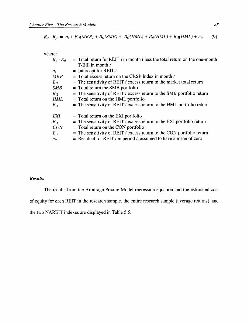
58
Rit - Rft = ai + Bil(MKP) + Bi2(SMB) + Bi3(HML) + Bi 3 (HML) + Bi3 (HML) + eit
where:Ri - Rf,
aiMKPBilSMBBi2HMLBi3
(9)
= Total return for REIT i in month t less the total return on the one-monthT-Bill in month t
= Intercept for REIT i= Total excess return on the CRSP Index in month t= The sensitivity of REIT i excess return to the market total return= Total return the SMB portfolio= The sensitivity of REIT i excess return to the SMB portfolio return= Total return on the HML portfolio= The sensitivity of REIT i excess return to the HML portfolio return
EXI = Total return on the EXI portfolioBi4 = The sensitivity of REIT i excess return to the EXI portfolio returnCON = Total return on the CON portfolioBi5 = The sensitivity of REIT i excess return to the CON portfolio returneit = Residual for REIT i in period t, assumed to have a mean of zero
Results
The results from the Arbitrage Pricing Model regression equation and the estimated cost
of equity for each REIT in the research sample, the entire research sample (average returns), and
the two NAREIT indexes are displayed in Table 5.5.
Chapter Five - The Research Models

Chapter Five - The Research Models
Table 5.5 - Arbitrage Pricing Model Regression ResultsR i -Rf = a i + B i] (MKP) + B i2 (SMB) + B 3 (HML) + B 4 (EXI) + B (CON) + e i
-0.182 0.606 0.405 0.585 -0.440 0.160-0.070 0.576 0.393 0.562 -1.053 -0.115
Office /Industrial
Duke-Weeks Realty Corporation -0.129 0.685 0.145 0.521 1.180 2.919Spieker Properties, Inc. 1.778 0.312 0.317 0.624 -6.550 -1.771Liberty Property Trust 0.025 0.667 0.302 0.448 -0.271 1.701Mack-Call Realty Corporation 0.456 0.652 0.474 0.459 0.656 0.505Highwoods Properties, Inc. -0.250 0.705 0.360 0.466 -0.616 2.341CarrAmerica Realty Corporation 0.464 0.864 0.431 0.800 -6.221 -3.657HRPT Properties Trust -0.836 0.764 0.036 0.716 0.535 1.159First Industrial Realty Trust, Inc. 0.504 0.680 0.406 0.236 -3.667 -1.829Koger Equity, Inc. 0.685 0.555 1.049 0.673 8.553 4.233Pacific Gulf Properties, Inc. 0.385 0.742 0.389 0.719 -0.677 0.807Keystone Property Trust 1.760 0.623 0.969 0.629 -0.497 2.076Average 0.440 0.659 0.443 0.572 -0.689 0.771
RetailKimco Realty Corporation 0.651 0.550 0.329 0.486 -3.902 -6.384General Growth Properties, Inc. 0.955 0.393 0.205 0.732 -6.222 1.415New Plan Excel Realty Trust, Inc. 0.475 0.502 0.299 0.545 1.509 -0.138Regency Realty Corporation 0.552 0.500 0.536 0.743 -1.545 3.385Developers Diversified Rlty Corp. 0.200 0.487 0.467 0.719 -4.829 0.423Macerich Company, The 0.249 0.642 0.506 0.665 -5.085 0.303Taubman Centers, Inc. 0.361 0.406 0.266 0.467 -2.284 1.688Realty Income Corporation -0.143 0.402 0.494 0.598 9.167 1.906CBL & Associates Properties, Inc. 0.148 0.181 0.375 0.375 2.300 1.860Chelsea GCA Realty, Inc. 0.472 0.638 0.708 0.894 -1.889 0.164Mills Corporation, The 0.334 0.735 0.360 0.768 -3.990 -3.294Glimcher Realty Trust -0.472 0.770 0.771 0.877 -2.337 -0.257Commercial Net Lease Realty, Inc -0.568 0.951 0.089 0.962 -3.034 -0.374JP Realty, Inc. -0.324 0.558 -0.085 0.463 -6.265 3.247Saul Centers, Inc. -0.044 0.487 0.379 0.666 2.213 3.781Crown American Realty Trust -0.486 0.682 0.611 0.787 -5.656 -8.485Mid-Atlantic Realty Trust 0.380 0.568 0.306 0.676 1.509 -2.188Acadia Realty Trust -1.515 0.502 0.301 0.425 -2.117 -1.805Kranzco Realty Trust -0.807 0.580 0.683 0.599 -0.389 2.165Ramco-Gershenson Properties Tr. -0.435 0.330 0.278 0.242 0.672 -0.864Malan Realty Investors, Inc. 0.924 0.205 0.336 0.393 -5.075 6.708Average 0.043 0.527 0.391 0.623 -1.774 0.155
Residential (Multifamily)Equity Residential Properties Tr. 0.476 0.729 0.203 0.598 -3.385 -4.326Apartment Investment & Mgmt. C( 1.591 0.529 0.344 0.571 -3.206 1.107Camden Property Trust 0.261 0.529 0.219 0.412 -3.766 1.188BRE Properties, Inc. 1.120 0.319 0.423 0.583 -2.817 -1.423Gables Residential Trust 0.651 0.333 0.173 0.354 -3.611 -3.976Essex Property Trust, Inc. 1.065 0.586 0.509 0.753 3.104 0.779Summit Properties Inc. 0.381 0.384 0.602 0.545 -1.926 -1.746Mid-America Apartment Cmtys -0.315 0.495 0.360 0.346 -0.967 1.644Town and Country Trust, The 0.296 0.617 0.377 0.395 1.252 -2.824Associated Estates Realty Corp. -1.751 0.540 0.443 0.543 4.318 4.813Average 0.378 0.506 0.365 0.510 -1.101 -0.476
DiversifiedVomado Realty Trust 1.731 0.624 0.649 0.964 -7.936 -1.562Crescent Real Estate Equities, Inc 0.129 1.082 0.631 0.809 -3.294 0.968Washington REIT -0.300 0.393 0.219 0.351 0.963 -1.997Colonial Properties Trust -0.306 0.632 0.327 0.601 2.014 -0.026Pennsylvania REIT -0.574 0.448 0.117 0.823 5.346 0.997Transcontinental Realty Investors -0.215 0.577 -0.012 0.300 0.603 0.886Boddie-Noell Properties, Inc. -0.129 0.251 0.386 0.441 0.987 -3.096Average 0.048 0.572 0.331 0.613 -0.188 -0.547
t- statisticsB4 B, t(a) t(B) t(B 2 ) t(B3) t(B 4 ) t(B5) R
2
-0.463 6.137 3.498 4.938 -0.237 0.093 0.49-0.178 5.828 3.391 4.736 -0.565 -0.066 0.47
-0.178 3.758 0.677 2.380 0.343 0.918 0.242.328 1.626 1.409 2.710 -1.810 -0.529 0.170.036 3.776 1.460 2.112 -0.081 0.552 0.240.627 3.570 2.215 2.095 0.191 0.159 0.26
-0.308 3.468 1.513 1.909 -0.161 0.660 0.220.688 5.101 2.172 3.938 -1.947 -1.238 0.39
-1.276 4.637 0.186 3.627 0.172 0.404 0.320.614 3.292 1.679 0.952 -0.942 -0.508 0.250.693 2.234 3.607 2.259 1.827 0.978 0.290.559 4.289 1.918 3.464 -0.208 0.268 0.301.349 1.902 2.525 1.599 -0.080 0.363 0.170.882 5.257 3.020 3.803 -0.291 0.353 0.42
0.938 3.151 1.608 2.322 -1.186 -2.098 0.241.338 2.191 0.974 3.401 -1.840 0.452 0.210.524 2.203 1.120 1.994 0.351 -0.035 0.120.849 3.062 2.800 3.792 -0.502 1.188 0.300.323 3.121 2.556 3.844 -1.642 0.156 0.290.365 3.742 2.519 3.229 -1.572 0.101 0.310.565 2.530 1.417 2.428 -0.755 0.604 0.16
-0.217 2.442 2.559 3.026 2.951 0.664 0.320.242 1.182 2.083 2.036 0.795 0.695 0.130.588 3.163 2.998 3.696 -0.497 0.047 0.290.327 2.866 1.198 2.496 -0.825 -0.737 0.17
-0.582 3.780 3.234 3.592 -0.609 -0.072 0.33-0.900 5.997 0.479 5.053 -1.014 -0.135 0.43-0.429 2.943 -0.381 2.038 -1.754 0.983 0.18-0.063 2.806 1.866 3.199 0.676 1.249 0.24-0.455 2.543 1.944 2.446 -1.118 -1.814 0.210.460 2.737 1.260 2.715 0.386 -0.605 0.18
-1.776 2.343 1.197 1.651 -0.524 -0.483 0.12-0.842 2.411 2.423 2.074 -0.086 0.516 0.19-0.679 2.054 1.475 1.254 0.222 -0.308 0.111.202 1.060 1.485 1.696 -1.394 1.992 0.180.109 5.290 3.350 5.210 -0.944 0.089 0.45
0.675 4.113 0.980 2.816 -1.013 -1.401 0.272.073 2.740 1.521 2.467 -0.882 0.329 0.170.340 2.741 0.967 1.780 -1.036 0.353 0.151.573 1.781 2.016 2.716 -0.835 -0.456 0.161.039 2.113 0.940 1.876 -1.216 -1.448 0.141.537 3.364 2.497 3.608 0.945 0.256 0.290.624 2.503 3.348 2.959 -0.666 -0.652 0.27
-0.472 2.944 1.830 1.717 -0.305 0.561 0.200.462 3.831 1.997 2.044 0.412 -1.006 0.28
-1.899 2.330 1.633 1.956 0.989 1.192 0.170.792 4.223 2.603 3.550 -0.487 -0.228 0.33
1.996 2.864 2.544 3.687 -1.931 -0.411 0.290.135 4.514 2.248 2.813 -0.729 0.232 0.33
-0.545 2.836 1.351 2.116 0.369 -0.827 0.17-0.533 4.378 1.936 3.471 0.741 -0.010 0.32-0.883 2.739 0.610 4.200 1.735 0.350 0.32-0.183 1.959 -0.034 0.851 0.109 0.173 0.07-0.171 1.322 1.739 1.941 0.276 -0.936 0.110.120 5.709 2.821 5.098 -0.100 -0.313 0.45
0.527 5.829 3.464 5.104 -0.645 0.038 0.48 11.98
REIT
59
NAREIT IndexAll REITsEquity REITs
Coefficientsa B, B2 B3
13.3711.98
18.281.39
14.9915.1215.644.67
16.736.46
30.0315.1816.3914.08
1.275.93
14.5215.287.718.25
10.5126.2214.7713.29
6.7513.2712.88
7.5819.92-0.7113.357.70
15.7910.3310.5011.19
5.5810.108.716.611.87
19.178.02
12.5111.8223.7310.81
3.7915.1310.2816.4620.9513.63
8.7112.71
--
--
--
-
TOTAL SAMPLE AVERAGE 0.201 0.559 0.389 0.587 -1.166 0.064

Chapter Five - The Research Models 60
The addition of the two macroeconomic variables to the regression model does not
improve the predictive ability of the model. The EXI factor is not significant at the 5% level for
any of the REITs in the sample, with one exception. The factor is significant at the 10% level for
only four of the REITs. It is interesting to note, however, that the sign of the coefficient is
negative in over 63% of the individual regressions, as well as in the regressions for the total
sample average and the NAREIT indexes. This may indicate that equity REITs do provide some
degree of a hedge against inflation. Notwithstanding, since the factor is not significant in the
model, the actual effect and its magnitude is inconclusive. The other macroeconomic factor,
CON, is also only significant at the 5% level for one REIT in the research sample, and two at the
10% level. The sign on this coefficient appears to be random.
The insignificance of the two additional variables results in a coefficient of determination
(R2) of 0.478, an improvement of only 0.004 over the FFM. The mechanics of the regression
equation make it impossible for the addition of more variables to result in a smaller R2. If the
additional variables are significant at all, the R2 should always increase. Hence, the increase in
our model of less than half of one percent is inconsequential.
Another indication of the lack of validity and reliability of the combined APM is the wide
variation in cost of equity estimates. The range of estimates is -0.71% (Mid-Atlantic Realty
Trust) to 30.03% (Koger Equity, Inc.). Obviously, a negative cost of equity is impossible
(although desirable). The model results in an estimate of less than 5.0% for five REITs in the
research sample, and over 20% for four of them.
Chapter Six - Conclusions & Recommendations for Further Research 61
CHAPTER SIX
Conclusions & Recommendations for Further Research
Project and asset valuation is central to the success of any firm. Unfortunately, the
process is plagued with uncertainty. First of all, there exists inaccuracy regarding the level of
future cashflow estimates. But even perfectly projected cashflows are subject to the uncertainty
pertaining to the correct discount rate, or "hurdle rate", used to compute the present value of an
asset or investment. This "hurdle rate" is often the estimate of a firm's cost of capital, or the
minimum rate of return the company can earn on existing assets and still meet the expectations
of its capital providers. The uncertainty in the discount rate is a function of the difficulty in
estimating the return expectations of equity holders, or the cost of equity capital.
Estimating the cost of equity capital for a firm is at once the most critical and the most
difficult element of most business valuations and capital expenditure decisions. The expected
returns on common equity have two components: (1) dividends or distributions, and (2) changes
in market value (capital gains or losses). Because these return expectations cannot be directly
observed, they must be estimated from current and past market evidence. Therefore, it is
necessary to look to the investment markets for the necessary data for estimating the cost of
capital for any company, security, or project.
This study examines three specific asset-pricing models in an effort to determine a
reliable pricing model that can be used in practice to effectively estimate the cost of equity
capital for Real Estate Investment Trusts (REITs). While this subject is important for all
industries, it has particular relevance for the REITs, as the current competitive environment has
Chapter Six - Conclusions & Recommendations for Further Research 62
forced many REITs to explore new methods of increasing earnings. Hence, it is vital that REITs
have an accurate benchmark on which to base new capital budgeting and investment decisions.
The first research model employed is the traditional CAPM, where the total excess
returns for each REIT in the sample are regressed against the total excess returns of the broad
market index. The second research model incorporates the two firm-specific factors developed
by Fama and French, SMB and HML. In the third model, two additional macroeconomic factors
are included to represent the change in expected inflation and the change in the risk premium.
Using factors that are of a pervasive macroeconimic nature is in line with the Arbitrage Pricing
Theory of Ross.
The results indicate that the Fama-French model is far superior to the other two models in
predicting excess total returns (cost of equity) for the research sample of equity REITs. This
conclusion is based upon a nonparametric test comparing the fitted R 2's from each of the
regressions. Furthermore, the range of cost of equity estimates seems rational given the specific
characteristics of equity REITs.
It is important to recognize that, despite the superiority of the FFM, it still an imprecise
measurement tool. While the coefficient of determination for the sample average regression
equation is much higher than that of the CAPM, the model still predicts less than half of the
variation of excess REIT returns. Moreover, the standard error of the average regression is
0.97%. Using standard convention of plus and minus two standard errors results in a total
estimate range of 11.36% to 15.26%. While the standard error is much less than for the CAPM,
the wide range for the discount rate will result in a large degree of uncertainty in the subsequent
asset or investment valuation.

Chapter Six - Conclusions & Recommendations for Further Research 63
Another issue which affects the validity and reliability of the FFM (as well as other
models) is the historical time period over which the factor risk premiums are calculated. The
risk premiums vary substantially over certain time periods, which results in very different cost of
equity estimates for the same firm. The general consensus is to use focus on long-term history,
as short-term observations may lead to illogical forecasts. Furthermore, using more observations
in the calculation results in a lower standard error of the estimate. Alternatively, there are
several arguments for focusing on recent history. For instance, return patters tend to change over
time, and the recent past may be most relevant to investors. In addition, the longer periods
include "major events" that have not repeated over time. This study uses data over a 27-year
period from January 1973 through December 1999 to calculate the factor risk premiums.
As with any asset-pricing (or cost of equity) model, the FFM is at best a guide - a starting
point for any valuation analysis. The ultimate discount rate must reflect the risks inherent in the
specific company, project, or asset, as well as the cash flows themselves. The results of this
analysis indicate that the Fama-French model provides a much better guide than the CAPM or
the particular Arbitrage Pricing Model used in this study when estimating the cost of equity
capital for REITs.
Recommendations for Further Research
While the REIT industry has been in existence since the 1960s, most of the growth has
occurred within the past decade. The modern REIT industry emerged through the IPO frenzy of
1993-94, when nearly two-thirds of all REITs in existence today were formed. The industry
continues to evolve as real estate markets mature and increased competition forces many firms to

Chapter Six - Conclusions & Recommendations for Further Research 64
sharpen their focus. The relative youth and volatility of the REIT industry brings into question
the validity of using historical data to predict future. As time passes, and the industry matures,
continued research should provide useful insight regarding expected REIT returns and cost of
equity capital.
Concerning the specific asset pricing models, the multifactor Arbitrage Pricing Model
presents a unique case in that the theory does not specify what risk factors, or how many, are to
be used. Most applications consider risk factors that are of a pervasive macroeconomic nature,
and existing research has indicated that five total factors seems to be the optimal number. In
addition to multiple factors, there are several options available to measure each factor. It is not
unreasonable to assume that the method of measurement employed can noticeably affect the
significance of a particular factor.
In this study, we chose the unanticipated Change in Expected Inflation (EXI) and the
Confidence Risk (CON) as our macroeconomic variables. This selection is based upon the
findings of previous studies, as well as availability of time-series data. Exploring the existence
and significance of other pricing factors, as well as ways to measure their effects, provides
another avenue for future study.
Continued research regarding the application of the Fama-French Model is also
important, especially with respect to the SMB and HML factors. For instance, the long-term
historical size premium that exists in ordinary equity returns has not been evident in recent
history. In fact, the premium is slightly negative for the past five years (1995 through 1999).
This may be due to the current bull market, or it may signal that the market is becoming more
efficient. Regardless, if the premium diminishes over time, so does the rationale for using the
SMB factor.
Bibliography 65
BIBLIOGRAPHY
Banz, R.W. "The Relationship between Return and Market Value of Common Stocks." Journalof Financial Economics (1981), 9, 103-26.
Basu, S. "The Relationship between Earnings, Yield, Market Value, and Return for NYSECommon Stocks: Further Evidence." Journal of Financial Economics (1983), 12, 129-56.
Berry, M., E. Burmeister, and M. McElroy. "Sorting out Risks Using Known APT Factors."Financial Analysts Journal (March/April 1988), 29-42.
Bhandari, L.C. "Debt/Equity Ratio and Expected Common Stock Returns: Empirical Evidence."Journal of Finance (1988), 43, 507-28.
Brealey, R.A. and S.C. Myers. Principles of Corporate Finance, 6 th Edition, Boston: IrwinMcGraw-Hill, 2000.
Brueggeman, W.B., J.D. Fisher. Real Estate Finance and Investments, 1 0 th Edition, Chicago:Irwin, 1997.
Burns, W. and D. Epley. "The Performance of Portfolios of REITs and Stocks." The Journal ofPortfolio Management (Spring 1982), 37-41.
Burmeister, E., R. Roll, and S.A. Ross. "A Practitioner's Guide to Arbitrage Pricing Theory." APractitioner's Guide to Factor Models, Charlottesville, VA: Research Foundation of theInstitute of Chartered Financial Analysts, 1994.
Chan, K.C., P.H. Hendershott, and A.B. Sanders. "Risk and Return on Real Estate: Evidencefrom Equity REITs." The Journal of the American Real Estate and Urban EconomicsAssociation (1990), 18, 431-52.
Chen, N.F. "Some Empirical Tests of the Theory of Arbitrage Pricing." Journal of Finance(December 1983) 38, 1393-414.
Chen, N.F., R. Roll, and S. Ross. "Economic Forces and the Stock Market." Journal of Business(July 1986), 383-403.
Chen, S., C. Hsieh, and B.D. Jordan. "Real Estate and the Arbitrage Pricing Theory:Macrovariables vs. Derived Factors." Real Estate Economics (1997) 25, 505-23.
Chen, S., C. Hsieh, T.W. Vines, and S. Chiou. "Macroeconomic Variables, Firm-SpecificVariables, and Returns to REITs." Journal of Real Estate Research (1998) 16, 269-77.
Copeland, T., T. Koller, and J. Murrin. Valuation: Measuring and Managing the Value ofCompanies, 2 nd Edition, New York: John Wiley and Sons, 1996.
Bibliography 65

Bibliography 66
Elton, E.J., M.J. Gruber, and J. Mei. "Cost of Capital Using Arbitrage Pricing Theory: A CaseStudy of Nine New York Utilities." Financial Markets, Institutions, and Instruments (August1994) 3, 46-73.
Fama, E.F. and J.D. MacBeth. "Risk, Return, and Equilibrium: Empirical Tests." Journal ofPolitical Economy (1973) 71, 607-36.
Fama, E.F., and K.R. French. "The Cross-Section of Expected Stock Returns." Journal ofFinance (1992) 47, 427-65.
Fama, E.F., and K.R. French. "Common Risk Factors in the Returns on Stocks and Bonds."Journal of Financial Economics (1993) 33, 3-56.
Fama, E.F., and K.R. French. "Industry Costs of Equity." Journal of Financial Economics(1997) 43, 153-93.
Garrigan, R.T. and J.F.C. Parsons. Real Estate Investment Trusts: Structure, Analysis, andStrategy. New York: McGraw-Hill, 1998.
Gobel, P.R. and K.S. Kim. "Performance Evaluation of Finite-Life Real Estate InvestmentTrusts." Journal of Real Estate Research (1989) 4, 57-69.
Gyourko J., and T. Sinai. "The REIT Vehicle: Its Value Today and in the Future." The Journalof Real Estate Research (1999) 18, 355-75.
Han, J. and Liang, Y. "The Historical Performance of Real Estate Investment Trusts." TheJournal of Real Estate Research (1995) 3, 235-62.
Howe, J. and J. Shilling. "REIT Advisor Performance." The Journal of the American Real Estateand Urban Economics Association (July 1990) 4, 479-99.
Kincheloe, S.C. "The Weighted Average Cost of Capital - The Correct Discount Rate."Appraisal Journal (January 1990), 88-95.
Kuhle, J.L. "Portfolio Diversification and Return Benefits - Common Stocks verses Real EstateInvestment Trusts." Journal of Real Estate Research (1987) 2, 1-9.
Lally, M. "The Accuracy of CAPM Proxies for Estimating a Firm's Cost of Equity." Accounting& Finance (May 1995), 63-72.
Ling, D. and A. Naranjo. "The Fundamental Determinants of Commercial Real Estate Returns."Journal of Real Estate Finance (1998), 13-24
Litt, J. and J.P. Mei. "A Risk Adjustment Model for REIT Evaluation." Journal of Real EstateFinance (1999), 9-19.
Bibliography 66
Bibliography 67
Maris, B.A. and F.A. Elayan. "Capital Structure and the Cost of Capital for Untaxed Firms: TheCase of REITs." The Journal of the American Real Estate and Urban Economics Association(1990) 18, 22-39.
Martin, J. and D. Cook. "A Comparison of the Recent Performance of Publicly Traded RealProperty Portfolios and Common Stocks." The Journal of the American Real Estate and UrbanEconomics Association (1991) 2, 184-210.
McCue, T.E. and J.L. Kling. "Real Estate Returns and the Macroeconomy: Some EmpiricalEvidence from Real Estate Investment Trust Data." Journal of Real Estate Research (1994) 9,277-87.
McIntosh, W., Y. Liang, and D. Tomkins. "An Examination of the Small-Firm Effect within theREIT Industry." Journal of Real Estate Research (1991) 6, 9-17.
Pratt, S.P. Cost of Capital: Estimation and Applications, New York: John Wiley & Sons, 1998.Reinganum, M.R. "Misspecification in Capital Asset Pricing: Empirical Anomalies Based onEarnings Yields and Market Values." Journal of Financial Economics (1981) 9, 19-46.
Riddiough, T. "Real Estate Capital Markets Lecture Notes." MIT, Spring 2000.
Roll, R., and S.A. Ross. "An Empirical Investigation of the Arbitrage Pricing Theory." Journalof Finance (1980) 35, 1073-103.
Rosenberg, B., K. Reid, and R. Lanstein. "Persuasive Evidence of Market Inefficiency." Journalof Portfolio Management (1985) 11, 9-17.
Ross, S.A. "The Arbitrage Theory of Capital Asset Pricing." Journal of Economic Theory(1976), 341-60.
Sagalyn, L. "Real Estate Risk in the Business Cycle: Evidence from Security Markets." Journalof Real Estate Research (March 1990) 5, 203-18.
Sharpe, W.F. "Capital Asset Prices: A Theory of Market Equilibrium Under Conditions ofRisk." Journal of Finance (1964) 19, 425-42.
Smith, K. and D. Shulman. "The Performance of Equity Real Estate Investment Trusts."Financial Analysts' Journal (September 1976), 61-66
Taggart, R.A., Jr. Quantitative Analysis for Investment Management, New Jersey: Prentice Hall,1996.
Titman, S. and A. Warga. "Risk and the Performance of Real Estate Investment Trusts: AMultiple Index Approach." The Journal of the American Real Estate and Urban EconomicsAssociation (1986) 14, 414-31.
Bibliography 67

Bibliography 68
Internet Resources:
www.birr.com
www.stls.frb.org
www.nareit.com
www.web.mit.edu/kfrench/www
wrds.wharton.upenn.edu

Appendix A 69
EQUITY REIT RESEARCH SAMPLE(Ranked by equity market capitalization; December 31, 1999)
Equity Market Capitalization (1)Ticker Current Property $ % of % of
Rank Company Symbols Exchange Subsector (Millions) Sector Industry
Office I/ Industrial1 Duke-Weeks Realty Corporation2 Spieker Properties, Inc.3 Liberty Property Trust4 Mack-Cali Realty Corporation5 Highwoods Properties, Inc.6 CarrAmerica Realty Corporation7 HRPT Properties Trust8 First Industrial Realty Trust, Inc.9 Koger Equity, Inc.
10 Pacific Gulf Properties, Inc.11 Keystone Property Trust
Sector Totals
Retail1 Kimco Realty Corporation2 General Growth Properties, Inc.3 New Plan Excel Realty Trust, Inc.4 Regency Realty Corporation5 Developers Diversified Realty Corporation6 Macerich Company, The7 Taubman Centers, Inc.8 Realty Income Corporation9 CBL & Associates Properties, Inc.
10 Chelsea GCA Realty, Inc.11 Mills Corporation, The12 Glimcher Realty Trust13 Commercial Net Lease Realty, Inc.14 JP Realty, Inc.15 Saul Centers, Inc.16 Crown American Realty Trust17 Mid-Atlantic Realty Trust18 Acadia Realty Trust19 Kranzco Realty Trust20 Ramco-Gershenson Properties Trust21 Malan Realty Investors, Inc.
Sector Totals
Residential (Multifamily)1 Equity Residential Properties Trust2 Apartment Investment & Mgmt. Co.3 Camden Property Trust4 BRE Properties, Inc.5 Gables Residential Trust6 Essex Property Trust, Inc.7 Summit Properties Inc.8 Mid-America Apartment Communities, Inc.9 Town and Country Trust, The
10 Associated Estates Realty CorporationSector Totals
Diversified1 Vornado Realty Trust2 Crescent Real Estate Equities, Inc.3 Washington Real Estate Investment Trust4 Colonial Properties Trust5 Pennsylvania Real Estate Investment Trust6 Transcontinental Realty Investors, Inc.7 Boddie-Noell Properties, Inc.
Sector Totals
DRESPKLRYCLI
HIWCREHRPFRKE
PAGKTR
KIMGGPNXLREGDDRMACTCO0
CBLCCGMLSGRTNNNJPRBFS
CWNMRRAKRKRTRPTMAL
EQRAIVCPTBREGBPESSSMTMAATCTAEC
VNOCEI
WRECLPPEITCIBNP
NYSENYSENYSENYSENYSENYSENYSENYSEAMEXNYSEAMEX
NYSENYSENYSENYSENYSENYSENYSENYSENYSENYSENYSENYSENYSENYSENYSENYSENYSENYSENYSENYSENYSE
NYSENYSENYSENYSENYSENYSENYSENYSENYSENYSE
MixedOfficeMixedOfficeOfficeOfficeOffice
IndustrialOffice
IndustrialIndustrial
Shopping CentersRegional Malls
Shopping CentersShopping CentersShopping Centers
Regional MallsRegional MallsFree StandingRegional Malls
Shopping CentersRegional MallsRegional MallsFree StandingRegional Malls
Shopping CentersRegional Malls
Shopping CentersShopping CentersShopping CentersShopping CentersShopping Centers
MultifamilyMultifamilyMultifamilyMultifamilyMultifamilyMultifamilyMultifamilyMultifamilyMultifamilyMultifamily
NYSENYSENYSENYSENYSENYSEAMEX
2,452.952,314.181,657.451,521.821,466.001,427.161,187.171,045.23
450.46418.80126.69
14,067.93
2,052.131,447.531,397.571,154.62
789.41708.79572.74553.21514.28470.09413.16305.93301.55275.64187.50144.14143.00117.56
93.0691.1369.17
6.3856.0244.3143.961
3.8163.7153.0902.7211.1731.0900.330
36.619
7.8535.5395.3484.4183.0212.7122.1922.1171.9681.7991.5811.1711.1541.0550.7180.5520.5470.4500.3560.3490.265
1.9991.8861.3511.2401.1951.1630.9670.8520.3670.3410.103
11.464
1.6721.1801.1390.9410.6430.5780.4670.4510.4190.3830.3370.2490.2460.2250.1530.1170.1170.0960.0760.0740.056
11,802.20 45.164 9.618
5,335.36 23.266 4.3482,662.01 11.608 2.1691,224.08 5.338 0.9981,013.66 4.420 0.826
605.79 2.642 0.494565.56 2.466 0.461441.03 1.923 0.359408.32 1.781 0.333283.09 1.234 0.231169.68 0.740 0.138
12,708.57 55.419 10.356
2,793.27 25.944 2.2762,233.13 20.741 1.820
535.38 4.973 0.436515.47 4.788 0.420194.04 1.802 0.158107.94 1.003 0.08848.61 0.451 0.040
6,427.85 59.701 5.238
TOTAL RESEARCH SAMPLE
(1) Equity market capitalization does not include operating partnership units or preferred stock.
45,006.55 -- 36.676

Apeni B7
Property Sectors and Relative Weights in the NAREIT Real-Time Index
(Ranked by equity market capitalization; December 31, 1999)
Equity Mkt. Cap.(1)# REIT $ millions %ofTotal
38 Office / IndustrialOffice (21)Industrial (10)Mixed (7)
50 RetailShopping Centers (31)Regional Malls (12)Free Standing (7)
28 ResidentialMultifamily (22)Manufactured Homes (6)
20 Diversified
15 Lodging / Resorts
4 Self Storage
13 Health Care
8 Specialty
24 MortgageHome Financing (14)Commercial Financing (10)
200
(1) Equity market capitalization does not include operating partnership units or preferred stock.
38,417.4023,904.28
8,485.426,027.71
26,131.7512,000.3711,213.242,918.13
25,027.1122,931.662,095.45
10,766.71
31.30719.4806.9154.912
21.2959.7799.1382.378
20.39518.687
1.708
8.774
5.293
3.823
3.791
3.652
1.6710.9020.769
100.000
6,495.11
4,691.61
4,652.17
4,480.86
2,050.061,106.63
943.43
122,712.77
Appendix B 70

71Annendix C
AVERAGE TOTAL RETURNSJanuary 1995 - December 1999
Average AverageTicker Current Monthly Annualized
Rank Company/ Index Symbols Exchange Return Return
IndexesCRSP Value-Weighted Index 2.08 24.96NAREIT Composite Index (All REITs) 0.68 8.17NAREIT Composite Index (Eq. REITs) 0.71 8.50
Office / Industrial1 Duke-Weeks Realty Corporation DRE NYSE 1.19 14.322 Spieker Properties, Inc. SPK NYSE 1.63 19.573 Liberty Property Trust LRY NYSE 1.17 14.004 Mack-Cali Realty Corporation CLI NYSE 1.55 18.585 Highwoods Properties, Inc. HIW NYSE 0.91 10.926 CarrAmerica Realty Corporation CRE NYSE 1.06 12.727 HRPT Properties Trust HRP NYSE 0.44 5.238 First Industrial Realty Trust, Inc. FR NYSE 1.42 17.029 Koger Equity, Inc. KE AMEX 1.98 23.73
10 Pacific Gulf Properties, Inc. PAG NYSE 1.39 16.6611 Keystone Property Trust KTR AMEX 2.46 29.52
Sector Average 1.38 16.57
Retail1 Kimco Realty Corporation KIM NYSE 1.09 13.062 General Growth Properties, Inc. GGP NYSE 1.01 12.143 New Plan Excel Realty Trust, Inc. NXL NYSE 1.38 16.534 Regency Realty Corporation REG NYSE 1.08 12.915 Developers Diversified Realty Corporation DDR NYSE 0.41 4.966 Macerich Company, The MAC NYSE 0.72 8.647 Taubman Centers, Inc. TCO NYSE 0.91 10.908 Realty Income Corporation O NYSE 1.14 13.689 CBL & Associates Properties, Inc. CBL NYSE 0.71 8.51
10 Chelsea GCA Realty, Inc. CCG NYSE 0.96 11.5411 Mills Corporation, The MLS NYSE 0.95 11.3612 Glimcher Realty Trust GRT NYSE 0.18 2.1613 Commercial Net Lease Realty, Inc. NNN NYSE 0.52 6.2114 JP Realty, Inc. JPR NYSE 0.33 3.9215 Saul Centers, Inc. BFS NYSE 0.87 10.4516 Crown American Realty Trust CWN NYSE (0.32) (3.79)17 Mid-Atlantic Realty Trust MRR NYSE 1.26 15.0718 Acadia Realty Trust AKR NYSE (0.86) (10.31)19 Kranzco Realty Trust KRT NYSE (0.05) (0.55)20 Ramco-Gershenson Properties Trust RPT NYSE 0.31 3.6721 Malan Realty Investors, Inc. MAL NYSE 1.06 12.68
Sector Average 0.65 7.80
Residential (Multifamily)1 Equity Residential Properties Trust EQR NYSE 1.27 15.242 Apartment Investment & Mgmt. Co. AIV NYSE 2.16 25.933 Camden Property Trust CPT NYSE 0.94 11.254 BRE Properties, Inc. BRE NYSE 1.28 15.315 Gables Residential Trust GBP NYSE 0.95 11.396 Essex Property Trust, Inc. ESS NYSE 2.04 24.487 Summit Properties Inc. SMT NYSE 0.67 8.038 Mid-America Apartment Communities, Inc. MAA NYSE 0.53 6.349 Town and Country Trust, The TCT NYSE 1.38 16.53
10 Associated Estates Realty Corporation AEC NYSE (0.50) (6.01)Sector Average 1.07 12.85
Diversified1 Vornado Realty Trust VNO NYSE 1.65 19.862 Crescent Real Estate Equities, Inc. CEI NYSE 1.35 16.183 Washington Real Estate Investment Trust WRE NYSE 0.49 5.874 Colonial Properties Trust CLP NYSE 0.81 9.685 Pennsylvania Real Estate Investment Trust PEI NYSE 0.45 5.386 Transcontinental Realty Investors, Inc. TCI NYSE 1.04 12.437 Boddie-Noell Properties, Inc. BNP AMEX 0.28 3.37
Sector Average 0.87 10.40
TOTAL RESEARCH SAMPLE 0.93 11.17