The Cost of Environmental Protection

Richard D. MorgensternWilliam A. PizerJhih-Shyang Shih

Discussion Paper 98-36

May 1998

1616 P Street, NWWashington, DC 20036Telephone 202-328-5000Fax 202-939-3460

c©1998 Resources for the Future. All rights reserved.No portion of this paper may be reproduced without permissionof the authors.

Discussion papers are research materials circulated by theirauthors for purposes of information and discussion. They havenot undergone formal peer review or the editorial treatmentaccorded RFFbooks and other publications.

The Cost of Environmental Protection

Richard D. Morgenstern, William A. Pizer, and Jhih-Shyang Shih

Abstract

Expenditures for environmental protection in the U.S. are estimated to exceed $150 billionannually or about 2% of GDP. This estimate, based on largely self-reported information, is oftencited as an assessment of the burden of current regulatory efforts and a standard against which theassociated benefits are measured. Little is known, however, about how well reported expendituresrelate to true costs. The potential for both incidental savings and uncounted burdens means thatactual costs could be either higher or lower than reported expenditures.

A significant literature supports the notion that increases in reported environmental expendi-tures probablyunderstateactual economic costs. Estimates of the true cost of a dollar increase inreported environmental spending range from $1.50 to $12.

This paper explores the relationship between reported expenditures and economic cost in themanufacturing sector in the context of a large plant-level data set at the four-digit SIC level. Weuse a cost function modeling approach which treats both environmental and non-environmentalproduction activities as distinct, unrelated cost minimization problems for each plant. We thenexplore the possibility that these activities are, in fact, related by including reported regulatoryexpenditures in the cost function for non-environmental output. Under the null hypothesis thatreported regulatory expenditures accurately measure the cost of regulation, the coefficient on thisterm should be zero.

In ten of eleven industries studied, including all of the heavily regulated industries, this nullhypothesis is accepted using our preferred fixed-effects model. Our best estimate, based on anexpenditure weighted average of the four most heavily regulated industries, indicates that an incre-mental dollar of reported environmental expenditure reduces non-environmental production costsby eighteen cents with a standard error of forty-two cents. This is equivalent to saying that totalcosts rise by eighty-two cents for every dollar increase in reported environmental expenditures.Using an alternative pooled model we find uniformly higher estimates. Although consistent withprevious results, we believe these higher estimates are biased by omitted variables characterizingdifferences among plants.

Summarizing, our results enable us to reject claims that environmental spending imposes largehidden costs on manufacturing plants. In fact, our best estimate indicates a modest though statisti-cally insignificantoverstatementof regulatory costs.

Key words: environmental costs, fixed-effects, translog cost model

JEL Classification No(s): C33, D24, Q28

ii

Contents

1 Introduction 1

2 Background 42.1 Distinguishing Reported Expenditures and Economic Costs . . . . . . . . . . . . . 42.2 The Potential for Overstatement . . . . . . . . . . . . . . . . . . . . . . . . . . . 62.3 Empirical Studies of PACE Data . . . . . . . . . . . . . . . . . . . . . . . . . . . 7

3 Model 93.1 General Approach . . . . . . . . . . . . . . . . . . . . . . . . . . . . . . . . . . . 103.2 Specification . . . . . . . . . . . . . . . . . . . . . . . . . . . . . . . . . . . . . 123.3 Accounting for Plant-Level Differences . . . . . . . . . . . . . . . . . . . . . . . 15

4 Measuring the Cost of Environmental Expenditures 194.1 Marginal Regulatory Cost . . . . . . . . . . . . . . . . . . . . . . . . . . . . . . . 204.2 Industry and Manufacturing Sector Estimates . . . . . . . . . . . . . . . . . . . . 234.3 Small Expenditure Industries . . . . . . . . . . . . . . . . . . . . . . . . . . . . . 25

5 Conclusion 27

A Data Sources 32

B Estimation 37B.1 Distinguishing Environmental and Non-Environmental Cost Shares . . . . . . . . . 38B.2 Parameter Validity . . . . . . . . . . . . . . . . . . . . . . . . . . . . . . . . . . 41

List of Figures

1 Fixed Effects versus Pooled Estimator . . . . . . . . . . . . . . . . . . . . . . . . 16

List of Tables

1 Offset Estimates – Large Expenditure Industries . . . . . . . . . . . . . . . . . . . 222 Offset Estimates – Small Expenditure Industries . . . . . . . . . . . . . . . . . . . 26A.1 Sample Size by Industry . . . . . . . . . . . . . . . . . . . . . . . . . . . . . . . 33B.2 Estimation results . . . . . . . . . . . . . . . . . . . . . . . . . . . . . . . . . . . 35B.3 Assessment of Model Consistency . . . . . . . . . . . . . . . . . . . . . . . . . . 39

iii

The Cost of Environmental Protection?

Richard D. Morgenstern, William A. Pizer, and Jhih-Shyang Shih1

1 Introduction

Expenditures for environmental protection in the U.S. are estimated to exceed $150 billion annually

or about 2% of GDP. This estimate, based on largely self-reported information, is often cited as an

assessment of the burden of current regulatory efforts and a standard against which the associated

benefits are measured. Little is known, however, about how well reported expenditures relate to

true economic costs. Reported expenditures in the manufacturing sector reflect expenses that the

plant manager identifies with environmental protection. Yet, the cost to society depends on the

resulting changes in total production costs and output prices. Increases in reported environmental

expenditures at the plant level may or may not result in dollar-for-dollar increases in production

costs. Specifically, the change in production costs depends on whether an increase in reported

environmental expenditures incidentally saves money, involves uncounted burdens, or has no other

consequence.2

Most research on this distinction between reported environmental expenditures and total pro-

duction costs has focused on the possibility that the former mayunderstatethe latter. Studies have

examined a number of issues, including the possible “crowding out” effect of environmental ex-

penditures on other productive investments, the importance of the so-called “new source bias” in

discouraging investment in more efficient facilities, and the potential loss of operational flexibility

1The authors are Visiting Scholar, Fellow, and Research Consultant, respectively, Quality of the Environment Divi-sion, Resources for the Future. (Morgenstern is also Associate Assistant Administrator, on leave, U.S. EnvironmentalProtection Agency). The authors gratefully acknowledge financial support from the U.S. Environmental ProtectionAgency (Cooperative Agreement No. 821821-01-4) and technical assistance from the Center of Economic Studies(CES), U.S. Bureau of the Census. Robert Bechtold, Arnold Reznek, and Mary Streitwieser at CES all providedhelpful assistance. At Resources for the Future, Raymond Kopp has been a continuing source of advice and support.Dallas Burtraw, Wayne Gray, Winston Harrington, Richard Newell, Paul Portney and Kerry Smith, along with otherseminar participants at RFF, EPA, the American Petroleum Institute, Harvard University, American University andthe University of Maryland provided helpful comments on an earlier draft. The authors alone are responsible for allremaining errors.

2Our focus on production costs as the correct measure of the resource cost associated with environmental protectionassumes that no monopolistic rents exist. If firms collect such rents, we would also need to consider the effect ofregulation on these rents (e.g., producer surplus) in order to estimate the economic cost of regulation.

1

associated with environmental controls. It has also been suggested that reported environmental

expenditures fail to capture significant managerial and other overhead costs allocable to environ-

mental protection. Data collected by industry, based on broader definitions of environmental ex-

penditure than those used by the Census Bureau, generally yields larger estimates.

In contrast, more limited research suggesting an overstatement of costs has explored the possi-

bility that there is complementarity between pollution control and other production activities.3 That

is, the costs of jointly producing conventional output and a cleaner environment may be lower than

if each were produced separately.4 Generally, only anecdotal information, along with some limited

case studies, support the notion that pollution control expenditures may be partially (or wholly)

offset by efficiency gains elsewhere in the firm.

Whether a $1 increase in reported environmental expenditures translates into changes in total

production costs of more or less than a $1 involves netting out a number of complex, often com-

peting effects. Frequently posed in terms of competitiveness or productivity, the prevailing view in

the economics literature is that an incremental $1 of reported environmental expenditures probably

increases total production costs by more than $1. Recent studies suggest that total costs may rise

by as much as $12 for every $1 of reported expenditures.

In our attempt to address this relationship between reported environmental expenditures and

true economic costs, we merge several large data sets containing plant-level information on re-

ported regulatory expenditures as well as prices and quantities of both inputs and outputs. The

sample consists of more than 800 different manufacturing plants for multiple industries at the 4-

digit SIC level over the period 1979-1991. We employ a cost-function modeling approach that

involves three basic steps. First, we distinguish between environmental abatement expenditures

and non-environmental production expenditures. Second, we model both the production of con-

ventional output and environmental services as distinct cost minimization problems and derive

3There is also a literature comparingex anteto ex postecosts. That is a related but distinct issue from the oneaddressed in this paper.

4Suppose a potential investment both increases efficiency and reduces pollution but has a slightly lower rate ofreturn than a firm’s other investment opportunities. When environmental regulation is imposed, the cost of compliancemight be relatively small since the necessary investment was almost profitable when the environmental benefits wereignored.

2

expressions for the resulting cost and factor input shares. Third, we estimate our cost modelinsert-

ing a term that reflects the possible impact of environmental expenditures on non-environmental

production. Under the null hypothesis that reported environmental expenditures accurately reflect

costs, the coefficient on this term should be zero. Our approach differs from previous work with

similar data by using a cost-function modeling approach that distinguishes the production of envi-

ronmental services and conventional output, by considering a larger number of industries, and by

paying particular attention to plant-specific effects.

Our main results, based on four large, heavily regulated industries, indicate large but statis-

tically insignificant variability across industrial sectors. We find that reported environmental ex-

penditures tend to generate offsetting savings in some industries and added burdens in others.

However, none of the estimated offsets is statistically significant from zero. Using our preferred

fixed-effects model, a weighted average of the four industries yields a best estimate of aggregate

savings in conventional production costs of eighteen cents for every dollar of reported incremental

pollution control expenditures, with a standard error of forty-two cents. This is equivalent to say-

ing that total production costs rise by eighty-two cents (one dollar minus eighteen cents) for every

dollar of reported environmental expenditures. Estimates based on an alternative, pooled model

consistently show smaller savings and larger additional burdens than the fixed-effects model. Al-

though the higher, pooled estimates are more consistent with previous work, we believe they are

biased by omitted variables characterizing differences among plants.

In the remainder of the paper, we first review the literature surrounding cost estimates of envi-

ronmental protection. We then present an industry level model of plant behavior in the presence

of environmental regulation using a cost function approach. In Section 4 we discuss the estima-

tion of this cost function and use the results to compute the marginal cost associated with reported

environmental expenditures. Section 5 offers a set of concluding observations. Details concerning

construction of the dataset and estimation of the model parameters are contained in the Appendix.

3

2 Background

2.1 Distinguishing Reported Expenditures and Economic Costs

The key issue addressed in this paper is the possible gap between the true cost of environmental

regulation and readily available, self-reported expenditure estimates. To obtain anaccurate mea-

sure of true economic cost, one can imagine plant managers providing accurate responses to the

following (hypothetical) question:

“Identify the increase in costs associated with your efforts to reduce environmentalemissions or discharges from your facility. In preparing your estimates, be sure to con-sider the extent to which environmental activities : (a) involve direct outlays of capitaland operating costs; (b) reduce other (i.e., non-environmental) capital and operatingcosts; (c) lead to cost-saving innovations; (d) affect operating flexibility; (e) crowd outnon-environmental investments; or (f) discourage purchase of new equipment becauseof differential performance requirements for new versus existing equipment. Includeestimates of the plant managers’ time and other overhead items associated with theseactivities. Exclude expenditures related to occupational health and safety. When pro-cess changes (as opposed to end-of-the pipe additions) are involved, allocate only thatportion of the costs attributable to environmental protection.”

Of course few firms possess the information to reliably answer such a complex and comprehen-

sive question. Instead, we have at our disposal the Pollution Abatement Costs and Expenditures

(PACE) Survey. Collected by the U.S. Census Bureau in most years 1973-1994, the PACE ques-

tionnaire asks a sample of manufacturing plants to provide information on capital and operating

expenditures, including depreciation, labor, materials, energy and other inputs – essentially item

(a) of our hypothetical question.5

PACE results have been regularly published by Census and represent, by far, the most compre-

hensive source of information on environmental expenditures. They form the basis of calculations

that annualized environmental costs exceed $150 billion (U.S. Environmental Protection Agency

5The Census Bureau ceased collecting PACE in1994 for budgetary reasons. The PACE questionnaire asks plantmanagers how expenditures compare to what they would have been in the absence of environmental regulation. Thisraises the issue of the appropriate baseline. Absent regulation, firms might still engage in some pollution control tolimit tort liability, maintain good relations with communities in which they are located, maintain a good environmentalimage, and other reasons. However, it is unclear whether survey respondents are able to determine what environmentalexpenditures would have been made in the absence of regulation.

4

1990).6 PACE data have been used as inputs in dynamic general equilibrium analyses to estimate

the long-run consequences of environmental regulation. These results indicate social costs which

are from 30 to 50 percent higher than reported annual expenditures (Hazilla and Kopp 1990; Jor-

genson and Wilcoxen 1990). PACE data have also been used to analyze the decline in productivity

growth observed during the 1970’s. For example, researchers have found that environmental regu-

lations accounted for 8 to 44 percent of the declines in total factor productivity observed in various

industries (U.S. Office of Technology Assessment 1994).

Despite the broad use of PACE data and the widespread presumption that it measures economic

costs, numerous issues distinguish PACE data from true economic costs. When firms report oper-

ating expenses, for example, it is unclear how they handle management time and other overhead

items. As discussed by Noreen and Soderstrom (1994), treating overhead as either completely

variable or completely fixed is generally wrong – leading to over- or understatement of costs, re-

spectively. Various studies also suggest that responses to items (d-f) in the hypothetical question

would likely raise estimates of costs above those implied by the expenditure data alone (for ex-

cellent surveys, see Jaffee, Peterson, Portney, and Stavins 1995; Schmalensee 1993). There is

some evidence, for example, that environmental investments may crowd out other investments by

firms (Rose 1983). Further, many environmental regulations mandate stringent standards for new

plants but effectively exempt older ones from requirements. This new source bias may discour-

age investment in new, more efficient facilities and thereby raise production costs (Gruenspecht

1982; Nelson, Tietenberg, and Donihue 1993). It has also been suggested that pollution control

requirements may reduce operating flexibility which, in turn, could also lead to higher costs (Joshi

et al. 1997). Industry estimates of pollution control expenditures, using broader definitions of cost

than those used by the Census Bureau, routinely generate higher estimates. One recent industry

estimate was almost double the PACE number (American Petroleum Institute 1996).

6The EPA estimates are somewhat higher than those developed by Census Bureau largely because: 1) EPA annu-alizes investment outlays (at a 7 percent discount rate) rather than directly reporting annual expenditures; and 2) theEPA data includes some programs not covered by Census, e.g., drinking water and Superfund.

5

2.2 The Potential for Overstatement

In contrast to items (d-f), (b) and (c) in the hypothetical survey question represent a very different

line of thinking. Item (b) addresses the argument that potential complementarities between con-

ventional production and environmental expenditures may offset part of the reported environmental

expenditures. Especially when process changes are involved (as opposed to end-of-the-pipe treat-

ment), the cost of jointly producing both conventional output and a cleaner environment may be

lower than the cost of producing them separately. Such complentarities might arise, for example,

from cost savings associated with recovered or recycled effluents. The PACE survey has attempted

to estimate these so-called offsets but they are among the items thought to be most subject to

measurement error (Streitweiser 1996).

Another complementarity story arises when the costs of shutting down a production line are

substantial. Once it becomes necessary to stop production in order to make environmentally mo-

tivated modifications, it is only natural that other, non-environmentally motivated projects might

also be undertaken. This “harvesting” of non-environmental projects alongside necessary environ-

mental ones reduces the expenses associated the non-environmental projects, leading to a comple-

mentarity.

Item (c) represents the notion that environmental requirements may stimulate plant managers

to innovate and thus may offset some of the added costs associated with environmental protection.

The underlying argument has its roots in the work of Leibenstein (1966) and others who have writ-

ten about suboptimal firm behavior. The application to environmental issues goes back at least to

Ashford, Ayers, and Stone (1985). The most recent discussion is associated with Porter (1991)

who claims that “environmental standards can trigger innovation that may partially or more than

fully offset the costs of complying with them” (Porter and Van der Linde 1995). In effect, the argu-

ment is that the complementarities between environmental activities and conventional production

(item b) combined with the induced innovations associated with environmental requirements (item

c) may actually exceed the direct expenditures associated with environmental protection (item a).

The empirical basis for assessing these claims is quite limited. A study by Meyer (1993), which

6

examines whether states with strict environmental laws demonstrate poor economic performance

relative to states with more lax standards, is frequently cited in support of the Porter hypothesis.

Althought the study found that states with stricter laws actually performed better, the paper sheds

little light on a possible causal relationship between regulation and economic performance because

it does not control for many of the factors relevant to a state’s economic performance. Various case

studies of particular plants have been conducted but problems of selection bias make it impossible

to generalize from the results (Palmer, Oates, and Portney 1995).

Most economists have been unsympathetic to Porter’s arguments because they depend on the

assumption that firms consistently ignore or are ignorant of profitable opportunities, including the

use of innovative technologies (Palmer and Simpson 1993). This skepticism does not preclude spe-

cific instances where government regulations may lead to cost savings, e.g., the well-known case

of controls on vinyl chloride emissions (Doniger 1978). Alternatively, others have conjectured that

environmental regulation could have the effect of lowering costs – at least at the industry level – by

forcing exceptionally inefficient plants to close and thereby expanding production at the remaining,

more efficient facilities (U.S. Office of Technology Assessment 1980). Still, these examples are

generally regarded as special cases and considered atypical of behavior in a competitive economy.

2.3 Empirical Studies of PACE Data

Actual plant-level responses to our hypothetical survey question would enable researchers to mea-

sure the relative importance of the various, often countervailing influences. Absent such detailed,

data, we can only estimate the net effect based on available PACE and Census information. Sev-

eral other papers have also attempted to do this. Work by Gray (1987) and Gray and Shadbegian

(1994) explored these issues in the context of growth accounting. Using a straightforward model

where environmental activities are entirely separate from conventional production, they show that

a 1% increase in the ratio of environmental expenditures to total costs should lead to a 1% fall

in measured total factor productivity. Any deviation from this one-for-one relation indicates joint

production; in their terminology, productivity effects. Their results indicate a more than one-for-

7

one fall in measured productivity, suggesting that the cost of regulation is understated by reported

environmental expenditures. In the steel industry, for example, they find a $3.28 increase in total

costs for every additional dollar of environmental expenditure.

Similar work by Joshi, Lave, Shih, and McMichael (1997) (hereafter, JLSM) focuses on the

steel industry over the period 1979-88. JLSM distinguish between thedirect effects of regulation

(i.e., the reported abatement expenditures) and theindirecteffects reflecting any difference between

reported expenditures and changes in total production cost.7 JLSM estimate a cost function in

which pollution abatement expenditures enter as a fixed output, finding that the indirect effects of

regulation are large – on the order of $7-12 for each $1 in reported expenditures.

Our approach differs from previous work with similar data by considering a larger number of

industries, using a cost-function modeling approach that distinguishes the production of environ-

mental services and conventional output, and paying particular attention to plant-specific effects.

We prefer this method to the growth accounting framework of Gray and Shadbegian because it

more closely resembles the plant-level decision problem. Namely, prices are fixed and the plant

seeks to minimize costs, making costs and factor inputs the endogenous quantities. The growth

accounting framework, in contrast, treats factor inputs as fixed and output as the endogenous

variables.8

In contrast to JSLM, we adopt a cost function approach that allows for the possibility of disjoint

environmental and non-environmental activities under our null hypothesis. Their joint modeling

approach, while flexible, implicity rules out the possibility that environmental activities are unre-

lated to conventional production activities. By extension, this also eliminates the possibility that

reported environmental expenditures exactly measure true economic costs.9

We distinguish ourselves from both the Gray and Shadbegian and JSLM studies, however, in

7Gray (1987) refers to these indirect effects as thereal effect of regulation.8This assumes that productivity shocks are uncorrelated with factor inputs and that the scale of regulatory expen-

ditures depends on the level of inputs rather than the level of output.9By modeling the log of total costs as a linear function of the log of reported regulatory expenditure, it is impossible

for the derivative of total cost with respect to regulatory expenditure to identically equal one in the JSLM framework.The derivative in levels depends on the ratio of total costs divided by regulatory expense which varies across obser-vations. We instead specify our relation in terms of the log ofnon-environmentalproduction costs so that a zerocoefficient on regulatory expense reflects complete separation of environmental and non-environmental production.

8

our treatment of differences among plants. While we are able to replicate their general results in

Section 4, we show that those results depend critically on strong assumptions about homogeneity

among plants.10 Specifically, they assume that differences in plant location, age and management

have no effect on either productivity or environmental expenditure – an assumption that seems

unlikely to be satisfied in practice. Allowing for such differences (by estimating a fixed-effects

rather than a pooled model) substantially reduces the estimated economic cost associated with an

incremental dollar of reported expenditures. Our results, in fact, allow us to statistically reject the

hypothesis that the economic cost of an additional dollar of reported environmental expenditure is

much more than one dollar.

3 Model

The most transparent way to measure the relation between changes in total costs and changes in

reported PACE expenditures would be to focus on two identical groups of plants, one of which

is randomly subject to higher regulatory standards. Using this data we could simply examine the

difference in average non-environmental production costs between the two populations and then

compare it to the difference in average reported PACE expenditures. The ratio of the differences

would reveal the degree, if any, to which the reported PACE data over- or understates true costs.

Since the two groups would be otherwise identical (due to randomization), this would yield an

unbiased estimate of any potential savings or uncounted burdens.

In the absence of such a transparent, randomized experiment, we are forced to construct a

more complete model of production. This model must adequately account for other factors besides

regulation which affect costs. If we fail to do this, the influence of these factors may be falsely

attributed to regulation.

An important source of such confounding influence may be unobservable productivity differ-

ences among plants. These differences, which might be related to geographical location, man-

10Gray and Shadbegian report results allowing for plant heterogeneity but argue that they are more likely to beaffected by measurement error. As we discuss in Section B.2, this is not necessarily the case and, even if it were, thereare other compelling reasons to prefer the results allowing for heterogeneity.

9

agement style, age, or other plant characteristics, could influence the level of both environmental

and non-environmental expenditures. Simple pooling of the data to estimate the cost implications

of higher reported PACE expenditures without controlling for these differences would be equiva-

lent to asking what happens when regulatory expenditures changealong withassociated changes

plant location, management style and age. To the extent that we are interested in the economic

cost of higher environmental expenditures holding plant characteristics constant, this constitutes

an omitted-variable bias.

Since our data set contains multiple observations for each plant, we have the ability to con-

sider fixed-effects models which explicitly accomodate plant-level differences in productivity. The

downside to this approach is that between-plant variation in costs will be ascribed to these fixed

effects. Thus, the uncounted effects of more expensive regulation are estimated solely by exam-

ining changes in non-environmental expendituresover timeassociated with changes in reported

PACE expendituresover time. If there are, in fact, no productivity differences among plants, this

approach leads to unnecessarily noisier and less efficient parameter estimates. This potential loss

of efficiency is the cost of protecting ourselves against omitted-variable bias.

3.1 General Approach

Our analytic approach involves three distinct steps. First, we distinguish between environmental

abatement expenditures and non-environmental production expenditures. This distinction allows

us to consider the null hypothesis that conventional, non-environmental production expenditures

are unaffected by PACE activities. Second, we model the production of both environmental ser-

vices and conventional output as distinct cost minimization problems and derive expressions for

the resulting cost and factor input shares. Third, we estimate our cost modelinsertinga term that

reflects the possible impact of environmental expenditures on non-environmental production. If

regulatory efforts and conventional production are, in fact, distinct, this term will not be statis-

tically significant and we would conclude that reported environmental expenditures are a good

assessment of the true costs. Conversely, if the inserted environmental expenditure variable is sig-

10

nificant, then one would conclude that reported environmental expenditures arenot an accurate

measure of the cost of environmental regulation.

Estimation of our cost model is complicated by two data limitations: We cannot separate ob-

served factor inputs into those used for abatement efforts and those used for conventional produc-

tions. Also, we do not observe a “level” of environmental output. These limitations lead us to

make stronger identifying assumptions but do not fundamentally hinder our approach.

The first step, separating total expenditures into abatement effort and conventional production,

allows us to focus squarely on the hypothesis of interest. Under the null hypothesis that reported

environmental expenditures accurately reflect the cost of environmental regulation, the remaining

expenditures on conventional production should be completely determined by the level of conven-

tional output, prices of inputs, a time trend, and possible idiosyncratic differences among plants.

This leads to the second step, where we derive distinct expressions for expenditures on both

conventional production and abatement based on cost minimizing behavior by plants. By adopting

a structural approach, with model parameters representing technological constraints rather than

simple correlations in the data, we have greater confidence that the parameters are invariant to

changes in regulatory policy. Our cost function approach also assumes output and prices are ex-

ogenous. The plant then chooses the cost-minimizing combination of endogenous inputs. This, in

turn, determines expenditures on abatement and conventional output.

Our cost function approach has two advantages over conventional production function ap-

proaches, which instead treats inputs as exogenous and outputs as endogenous. First, we avoid

regressing output on regulatory expenditure which may be biased if the scale of output influences

regulatory costs.11 Second, we take advantage of the first order conditions for cost minimization

to impose additional restrictions on our parameters and improve estimation efficiency.

The third step of our analysis allows for potential economies of scope.12 Specifically, we in-

sert regulatory expenditures into our model of conventional, non-environmental production costs.

11Gray and Shadbegian (1994), for example, find that scaling abatement expenditures by output tends to bias theircost estimates upward.

12See Bailey and Friedlaender (1982).

11

This gives us an idea, loosely speaking, of the possible complementarities involved in the joint

production of conventional output and environmental activities. To the extent that environmental

activities are completely disjoint from regular production, the coefficient on regulatory expendi-

tures will be zero. In that case, the marginal economic cost of an additional dollar of environmental

expenditures will be entirely reflected by environmental expenditures alone and will exactly equal

one dollar.

If, however, environmental expenditures somehow complement conventional production, the

marginal cost could be less than a dollar. As noted, such complementarities might arise from

process changes which were almost profitable even without environmental considerations, from

benefits associated with recovered and recycled effluents, or from unforeseen spillovers caused

by regulatory activities. Alternatively, such efforts might impose additional, uncounted costs. The

possible crowding out of productive investments, higher administrative costs, and loss of flexibility,

for example, are presumably not counted in the measure of reported regulatory expenditures and

could lead to a marginal economic cost exceeding one dollar.

3.2 Specification

We now explain the key technical aspects of our model. In each periodt we assume each planti

wishes to minimize the cost associated with producing a given quantity of conventional outputY .

The functionFi,t(·) defines a production technology involvingY coupled with inputs of capital,

labor, energy, and materials. In particular,Fi,t(·) = 0 is the productionfrontier andFi,t(·) < 0

describes feasible but inefficient input/output combinations.13 The production function is indexed

over both plantsi and timet to allow for exogenous time trends in productivity as well as differ-

ences between plants.

13That is, given any feasible production combination it is always possible to use more inputs or produce feweroutputs by simply discarding the excess. However, unless some prices are zero this will not be efficient.

12

The cost minimization performed by the plant is given by:

PC = minK,L,E,M

PkK + PlL + PeE + PmM

such thatFi,t(Y,K, L,E,M) ≤ 0 with Y fixed,

(1)

wherePk, Pl, Pe, andPm represent prices of capital, labor, energy and materials, respectively, and

PC is the production cost associated withY .

The minimization in (1) defines a cost functionPC = Gi,t(Y, Pk, Pl, Pe, Pm).14 We specify

the cost function to be of the translog functional form:15

log(PC) = αi + α′i,x ·X +1

2X ′βxX + αr logR (2)

whereX = {logY, logPk, logPl, log Pe, log Pm, t}′, αi,x = {αy, αi,k, αi,l, αi,e, αi,m, αt}′, βx =[βy βk βl βe βm βt

], βy = {βyy, βyk, βyl, βye, βym, βyt}′, etc., andR is regulatory expenditure.

Note that we have assumed that plant differences as well as a time trend may change overall pro-

ductivity and bias the factor shares (see factor share equations below). We have also added a term

(αr logR) reflecting the possible influence of regulatory expenditures on conventional production

costs. Our null hypothesis is that the coefficientαr should be zero and that reported regulatory ex-

penditures accurately reflect the cost of environmental regulation. That is, PACE activities should

have no effect on non-environmental production costs.

Taking the first derivatives of this log cost function with respect to log prices yields expressions

for the associated factor shares by Shepard’s Lemma:

vk,y = αi,k + β ′kX

vl,y = αi,l + β ′lX

ve,y = αi,e + β ′eX

vm,y = αi,m + β ′mX

wherevk,y, vl,y, ve,y andvm,y are the input cost shares for capital, labor, energy and materials,

14For a general discussion of cost functions see Varian (1992).15See Diewert and Wales (1987) for a discussion of the translog and other flexible functional forms.

13

respectively, associated with producingY units of output, andβk = {βky, βkk, βkl, βke, βkm, βkt}′,

etc. As noted above, our specification allows for plant specific differences in factor demand.16

Normally, we would proceed with the simultaneous estimation of both the cost function (2)

and the share equations. However, the cost shares associated withY production costs (vk,y, vl,y,

etc.) are not, in fact, observed. Instead, we observe the cost shares associated with both production

costsandabatement costs. These “aggregate” cost shares are a weighted average of production and

abatement cost shares. The aggregate cost shares will not equal the production cost shares except

under the very restrictive assumption that the technology for producting outputY and abatement

are almost identical.

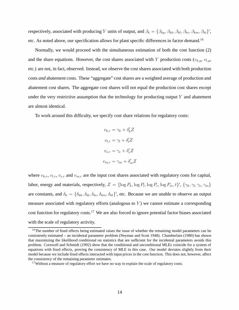
To work around this difficulty, we specify cost share relations for regulatory costs:

vk,r = γk + δ′kZ

vl,r = γl + δ′lZ

ve,r = γe + δ′eZ

vm,r = γm + δ′mZ

wherevk,r, vl,r, ve,r andvm,r are the input cost shares associated with regulatory costs for capital,

labor, energy and materials, respectively,Z = {logPk, logPl, logPe, logPm, t}′, {γk, γl, γe, γm}

are constants, andδk = {δkk, δkl, δke, δkm, δkt}′, etc. Because we are unable to observe an output

measure associated with regulatory efforts (analogous toY ) we cannot estimate a corresponding

cost function for regulatory costs.17 We are also forced to ignore potential factor biases associated

with the scale of regulatory activity.

16The number of fixed effects being estimated raises the issue of whether the remaining model parameters can beconsistently estimated – an incidental parameter problem (Neyman and Scott 1948). Chamberlain (1980) has shownthat maximizing the likelihood conditional on statistics that are sufficient for the incidental parameters avoids thisproblem. Cornwell and Schmidt (1992) show that the conditional and unconditional MLEs coincide for a system ofequations with fixed effects, proving the consistency of MLE in this case. Our model deviates slightly from theirmodel because we include fixed effects interacted with input prices in the cost function. This does not, however, affectthe consistency of the remaining parameter estimates.

17Without a measure of regulatory effort we have no way to explain the scale of regulatory costs.

14

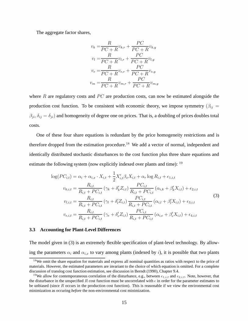
The aggregate factor shares,

vk =R

PC +Rvk,r +

PC

PC +Rvk,y

vl =R

PC +Rvl,r +

PC

PC +Rvl,y

ve =R

PC +Rve,r +

PC

PC +Rve,y

vm =R

PC +Rvm,r +

PC

PC +Rvm,y

whereR are regulatory costs andPC are production costs, can now be estimated alongside the

production cost function. To be consistent with economic theory, we impose symmetry(βij =

βji, δij = δji) and homogeneity of degree one on prices. That is, a doubling of prices doubles total

costs.

One of these four share equations is redundant by the price homogeneity restrictions and is

therefore dropped from the estimation procedure.18 We add a vector of normal, independent and

identically distributed stochastic disturbances to the cost function plus three share equations and

estimate the following system (now explicitly indexed over plants and time):19

log(PCi,t) = αi + αi,x ·Xi,t +1

2X ′i,tβxXi,t + αr logRi,t + ε1,i,t

vk,i,t =Ri,t

Ri,t + PCi,t(γk + δ′kZi,t)

PCi,tRi,t + PCi,t

(αi,k + β ′kXi,t) + ε2,i,t

vl,i,t =Ri,t

Ri,t + PCi,t(γl + δ′lZi,t)

PCi,tRi,t + PCi,t

(αi,l + β ′lXi,t) + ε3,i,t

ve,i,t =Ri,t

Ri,t + PCi,t(γe + δ′eZi,t)

PCi,tRi,t + PCi,t

(αi,e + β ′eXi,t) + ε4,i,t

(3)

3.3 Accounting for Plant-Level Differences

The model given in (3) is an extremely flexible specification of plant-level technology. By allow-

ing the parametersαi andαi,x to vary among plants (indexed byi), it is possible that two plants

18We omit the share equation for materials and express all nominal quantities as ratios with respect to the price ofmaterials. However, the estimated parameters are invariant to the choice of which equation is omitted. For a completediscussion of translog cost function estimation, see discussion in Berndt (1990), Chapter 9.4.

19We allow for contemporaneous correlation of the disturbance, e.g., betweenε1,i,t andε2,i,t. Note, however, thatthe disturbance in the unspecifiedR cost function must be uncorrelated withε in order for the parameter estimates tobe unbiased (sinceR occurs in the production cost function). This is reasonable if we view the environmental costminimization as occuringbeforethe non-environmental cost minimization.

15

Figure 1: Fixed Effects versus Pooled Estimatora

0 0.5 1 1.5 20

0.5

1

1.5

2

plant 1 obs.

plant 2 obs.

pooled regression line fixed-effect

regression line

reported environmental expenditure ($)

non-

envi

ronm

enta

l pro

duct

ion

cost

($)

aThis is a stylized representation of the model given in Equa-tion (2). It emphasizes the role of fixed effects but ignores othercovariates besides regulation as well as the log-log specification.

producing the same amount of output and facing the same input prices may have different produc-

tion costs and may use different combinations of inputs. Requiring some of these parameters to be

similar across plants then allows us to explore more restrictive models.

We could assume, for example, that there is no variation in any of theα’s across plants. That

would be the case if all plants shared exactly the same production technology. Under this assump-

tion, we could estimate the model by simply pooling the data and ignoring the panel structure (i.e.,

multiple observations for each plant).

To estimate the full model, we take advantage of the panel structure of the data, allow theα’s to

differ and estimate them along with the other parameters. We do this by adding dummy variables

for each plant in both the cost function and share equations and otherwise following the same

procedure as before.20

Figure 1 illustrates the potential discrepancy between these assumptions. Consider data from

two plants with six observations of production costs and regulatory expenditures for each. As

20The dummy variables appearing the share equations also appear in the cost function interacted with the corre-sponding prices.

16

drawn, there is a negligible effect of rising regulation on production costs for both plant 1 (denoted

by ◦) and plant 2 (denoted by×) viewed separately. If we view each plant separately – but require

increased environmental expenditures to have the same incremental effect – it would appear that

there is a roughly $0.20 decrease in production costs for every $1 increase in regulation. That is,

costs areoverstatedby reported expenditures. This is the fixed-effects estimate.

However, plant 1 has, on average, $0.50 more regulation than plant 2 and, on average, $1

more production costs – an increase of $2 in production costs per dollar of regulation. Pooling

the data, in effect averaging the zero-for-one fixed-effects relation with this two-for-one relation,

we estimate a pooled slope coefficient of 1.5. That is, based on the pooled estimate, costs are

substantiallyunderstatedby reported expenditures (by nearly 150%).

If there was no discrepancy between these two relations – that is, the relation among plant

means versus the relation among observations for each plant – then the fixed-effects and pooled

slope estimates would be roughly the same. Visually, the data points in Figure 1 would lie along

the same (dotted) line, rather than along two different (solid) lines. In this scenario, the pooled

estimator would be preferred since it uses more information (the relation between plant means)

than the fixed-effects estimator. This is especially important if there is more variation between

plants than within plants, as is usually the case.21

When there is a discrepancy, as illustrated in Figure 1 and as we find in our data, it is not imme-

diately obvious which of the two slope estimates – the fixed-effects or the pooled – is preferred.22

If we believe that the differences between plants are actuallycausedby differences in regulation,

then the pooled estimator is appropriate. Suppose, for example, that both regulatory expenditures

and total costs differ by plant location. In such a scenario, firms might only be willing to select

locations with higher regulatory expenditures if the other costs at that location were lower, at least

partially offsetting the higher regulatory costs. In that case, we might be interested in a slope

coefficient which included the indirect effect of higher regulation on total cost via the choice of

21See Table 2 in Gray and Shadbegian (1994).22We statistically reject the hypothesis that the intercepts are the same in every industry and at any reasonable level

of significance. See discussion in Appendix B.

17

plant location. This would correspond to the pooled estimate, where variation between plants, e.g.,

location, is used to identify the effect of regulation. The fixed-effect estimate, in contrast, ignores

this variation by controlling for all fixed (i.e., time invariant) differences among plants. In light of

this distinction, we might view the pooled estimate, which allows plant characteristics to change,

as along-runelasticity and the fixed-effects estimate, which holds constant differences between

plants, as ashort-runelasticity.23

There are three reasons why this scenario where regulation causes plant differences is inappro-

priate and why we instead prefer the fixed-effects model. First, it seems that there are many more

plant characteristics which are likely to influence regulatory costs rather than be influenced by it.

If firms choose their plant locations without regard for regulatory costs, even though regulatory

differences exist, it would be incorrect to compute an estimator which insinuated that regulation

affects location, rather than the other way around.24 Considering characteristics like age and man-

agement style, it becomes even more apparent that plant differences in regulatory expenditure are

more likely to be an effect than a cause of other plant differences. If environmental expenditures

are, in fact, affected by factors like plant age, location and management, the pooled estimator will

suffer from omitted-variable bias while the fixed-effects estimator will remain unbiased.

The second reason for preferring the fixed-effects model is an empirical one. As discussed in

Section 4, the pooled estimates are uniformlylarger than the fixed-effects estimates (as depicted

in Figure 1). If the purpose of the pooled estimator is to capture the increased flexibility over the

long run, the pooled slope estimate should instead besmaller. Thus, there are empirical reasons to

reject the pooled results.

Finally, even if we decide to estimate a regulatory effect which includes effects transmitted via

differences in plant characteristics, it would be inappropriate to simply pool the data as described.25

23Caves, Christensen, Tretheway, and Windle (1985) use this distinction to differentiate returns to scale from returnsto density in the U.S. railroad industry. Assuming the track network used by firms is fixed over time, they use a fixed-effects model to estimate return to density, holding network fixed, and a random-effects (e.g., pooled) model to estimatereturn to scale, allowing network size to vary.

24Bartik (1988), Bartik (1989), Friedman, Gerlowski, and Silberman (1992), Levinson (1992) and McConnell andSchwab (1990) all find small or insignificant effects of regulation on plant location.

25That is because differences in regulatory expenditures are unlikely to explainall the differences among plants,leaving a random, unexplained difference in cost which is common among the observations of a given plant. The pa-

18

Instead, a random-effects model would be appropriate (Mundlak 1978). The random-effects es-

timator, however, continues to suffer from the first two criticisms, i.e., omitted variable bias and

empirical incongruity with theory, again recommending the fixed-effects approach.26

4 Measuring the Cost of Environmental Expenditures

To determine the relationship between environmental expenditures and actual cost we estimate the

cost function and share equations derived in the previous section. The measure that concerns us –

the potential influence of environmental expenditures on non-environmental production costs – is

then determined from the estimated parameters.

In particular, the parameterαr measures the elasticity of non-environmental production costs

with respect to reported environmental expenditures. Multiplying this estimated elasticity by the

ratio of non-environmental costs to environmental expenditures for a particular plant reveals the

dollar change in non-environmental costs for a dollar change in reported environmental expendi-

tures. We refer to this quantity as the non-environmental costoffset. Adding one to this number

reveals the dollar change in total costs (environmental+ non-environmental) for a dollar change

in reported environmental costs. We refer to this quantity as themarginal costof reported environ-

mental expenditures.

The cost function and share equations given in (3) are estimated using maximum likelihood.

The resulting parameter estimates are reported in Table B.2 and described in Appendix B. It is

interesting to note that while just over half of the estimated parameters are significantly different

from zero,αr is significant in only one of the eleven industries.27 This immediately suggests that

there will be little evidence supporting the hypotheses of either understatement or overstatement

of regulatory costs.

rameterαi in this case would be a randomly distributed variable. While a simple pooled estimator would be consistentand unbiased, it would not be efficient nor would the standard errors be correct.

26There are potentially two opposing econometric reasons one might prefer the random-effects model over thefixed-effect model – measurement error and endogeneity. This is discussed in Appendix B.2.

27The results in the one significant industry, motor vehicles, are questionable based on the unrealistically largeestimate of $25 in additional, uncounted costs for every dollar of reported costs.

19

These results also indicate that our flexible modeling approach captures significant features of

the data. Tests that the fixed effects in each equation are zero, for example, are strongly rejected by

likelihood ratio tests.28 Therefore, alternative approaches which assume a simpler relation between

regulation and total costs may be misspecified.

4.1 Marginal Regulatory Cost

We examine the connection between environmental expenditures and total costs in terms of marginal

changes around the observed level of expenditures. In other words, we estimate the associated

change in total costs if current reported environmental expenditures rise by one dollar. An al-

ternative and different question is what fraction ofexistingreported expenditures actually reflect

existingeconomic costs – an average cost measure. Unfortunately, this is a more complex question

because it requires us to determine the relationship between reported expenditures and economic

costs, not only over the range of expenditures which we observe in the data, but all the way back

to zero expenditures. Such an extrapolation would not be credible. We do believe, however, that a

marginal cost considerably higher or lower than one would suggest a similar directional effect for

the average cost relation.

To calculate marginal cost, we differentiate the cost function in Equation (2) with respect to

regulatory expendituresR. This yields an estimate of non-environmental offset,O, associated with

an increase in reported environmental expenditure,

∂PC

∂R= O =

PC

Rαr (4)

wherePC is non-environmental production cost,R is regulatory expenditure, andαr is a param-

eter estimate from the cost function in Equation (2). Intuitively, this measure reveals the degree to

which additional environmental expenditures affect non-environmental expenditures. If this deriva-

tive is near zero, increases in reported expenditures are, in fact, a good measure of the additional

economic burden of further regulation. If the derivative is not equal to zero, such expenditures

28In each test, we compare the difference in the maximized log-likelihood between thepooled and fixed effectsmodels, multiplied by two, to a chi-squared distribution with4(n− 1) degrees of freedom, wheren is the number offirms in the sample and4(n− 1) is the number of additional restriction imposed by the pooled model.

20

misrepresent incremental costs, with offset values greater than zero indicating an understatement

of true costs and offset values less than zero an overstatement.

UsingO, we can also compute marginal costsMC = ∂(PC + R)/∂R = 1 + O. That is, the

change intotal costs associated with a change in reported regulatory expenditure. This measure

is useful because it summarizes the true cost associated with an incremental dollar of reported

environmental expense.

Since the value ofO computed in (4) depends on observation specific values ofPC andR,

these offset measures will vary from observation to observation. In order to compute an aggregate

answer, summarizing the offset at the industry or sectoral level, we have to make assumptions

about how to weight these different values. Conceptually, we are deciding how an increase in ag-

gregate regulatory expenditures would likely be allocated among firms in the sample. We could

compute a simple arithmetic average over all the observations. However, this would amount to

dividing up additional expenditures evenly among all observations – even though some plants cur-

rently have much lower regulatory expenditures than others. A more plausible alternative would be

to consider the aggregate offset of raising environmental expenditures across plantsin proportion

to each plant’s current expenditures.29 That is, plants with small expenditures would have small in-

creases and plants with large expenditures would have large increases. Such a calculation involves

a weighted average where the weights correspond to the level of each observation’s regulatory

expenditure:30

Oagg =∑i,t

(Ri,t∑j,sRj,s

)·Oi,t (5)

Aggregate marginal cost then equals one plus the computed value ofOagg.

21

Table 1: Offset Estimates – Large Expenditure Industries(standard errors are in parentheses)

Industry:

pu

lpan

dp

aper

pla

stic

s

pet

role

um

stee

l

cro

ss-in

du

stry

aver

age

Full sample# of obs. 615 404 717 536

➀fixed –0.36 –0.80 –0.22 0.41 –0.18effect (0.26) (0.56) (0.76) (0.42) (0.42)

➁pooled –0.03 –0.33 2.47∗ 2.28∗ 1.73∗

(0.23) (0.49) (0.62) (0.33) (0.34)

weight† 0.130 0.089 0.430 0.166 0.816

†Ratio of expenditures in each industry to eleven-industry total. This weight is used to compute cross-industryaverages. See footnote 31 in the text concerning calculationof the weights.∗Significant at the 5% level.

22

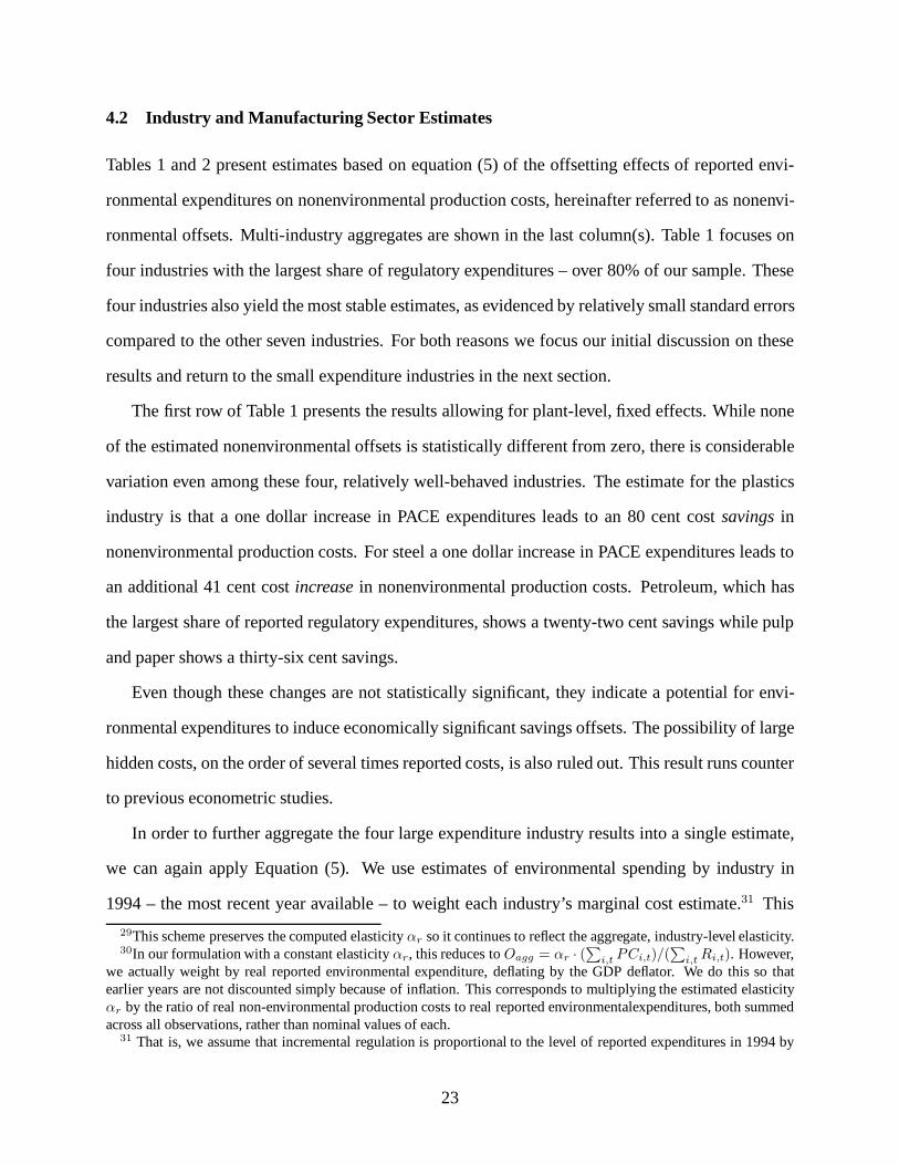
4.2 Industry and Manufacturing Sector Estimates

Tables 1 and 2 present estimates based on equation (5) of the offsetting effects of reported envi-

ronmental expenditures on nonenvironmental production costs, hereinafter referred to as nonenvi-

ronmental offsets. Multi-industry aggregates are shown in the last column(s). Table 1 focuses on

four industries with the largest share of regulatory expenditures – over 80% of our sample. These

four industries also yield the most stable estimates, as evidenced by relatively small standard errors

compared to the other seven industries. For both reasons we focus our initial discussion on these

results and return to the small expenditure industries in the next section.

The first row of Table 1 presents the results allowing for plant-level, fixed effects. While none

of the estimated nonenvironmental offsets is statistically different from zero, there is considerable

variation even among these four, relatively well-behaved industries. The estimate for the plastics

industry is that a one dollar increase in PACE expenditures leads to an 80 cent costsavingsin

nonenvironmental production costs. For steel a one dollar increase in PACE expenditures leads to

an additional 41 cent costincreasein nonenvironmental production costs. Petroleum, which has

the largest share of reported regulatory expenditures, shows a twenty-two cent savings while pulp

and paper shows a thirty-six cent savings.

Even though these changes are not statistically significant, they indicate a potential for envi-

ronmental expenditures to induce economically significant savings offsets. The possibility of large

hidden costs, on the order of several times reported costs, is also ruled out. This result runs counter

to previous econometric studies.

In order to further aggregate the four large expenditure industry results into a single estimate,

we can again apply Equation (5). We use estimates of environmental spending by industry in

1994 – the most recent year available – to weight each industry’s marginal cost estimate.31 This

29This scheme preserves the computed elasticityαr so it continues to reflect the aggregate, industry-level elasticity.30In our formulation with a constant elasticityαr, this reduces toOagg = αr · (

∑i,t PCi,t)/(

∑i,tRi,t). However,

we actually weight by real reported environmental expenditure, deflating by the GDP deflator. We do this so thatearlier years are not discounted simply because of inflation. This corresponds to multiplying the estimated elasticityαr by the ratio of real non-environmental production costs to real reported environmentalexpenditures, both summedacross all observations, rather than nominal values of each.

31 That is, we assume that incremental regulation is proportional to the level of reported expenditures in 1994 by

23

approach yields an aggregate estimate of nonenvironmental offsets of eighteen cents for every

dollar of increased reported regulatory expenditures, with a standard error of forty-two cents.32

Thus, our best estimate of the economic cost of a dollar increase in PACE expenditures is only

eighty-two cents (one dollar minus eighteen cents). Based on a 95% confidence interval, the true

economic cost ranges from negative two cents to positive $1.68. While this confidence interval is

quite large, it again indicates that extremely large values (> $1.68), are unlikely.

In contrast to the first row of estimates in Table 1 – which is based on the fixed effects model

– the second row of estimates is based on a pooled model. Unlike the fixed effects approach, the

pooled model assumes that the nonenvironmental offsets are completely explained by the included

right-hand side variables. This means that the effect of any omitted variables will be attributed to

the included right-hand side variables. This confounding of different effects potentially biases the

environmental offset estimates.

Interestingly, the pooled estimates are higher than the fixed-effects estimates for all four indus-

tries, significantly so in petroleum and steel. The (weighted) average environmental offset, driven

heavily by large increases in the petroleum and steel industries, rises to positive $1.73 per dollar of

PACE expenditures, with a standard error of $0.34. Based on this pooled model, the total economic

costs of a marginal dollar of reported environmental expenditures is $2.73 ($1.00 plus $1.73). The

pooled estimate is not only much higher, it is also in line with previous estimates concerning the

cost of regulation. Joshi et al. (1997) report an estimate of $7-12 for the steel industry using a cost

function modeling approach. Based on a growth accounting model, Gray and Shadbegian (1994)

find marginal costs of $1.74, $1.35 and $3.28 for paper mills, oil refineries and steel mills, respec-

tively. Both studies pool their data, although Gray and Shadbegian (1994) also report results for a

fixed-effects model that, like our fixed-effects results, are uniformly lower.33

industry. Withineach industry incremental regulation is allocated toeach observation in our multi-year sample inproportion to that observation’s real regulatory expenditure.

32Note that with a weight of0.430/0.816, petroleum plays a key role in determining the aggregate estimate.33$0.55, $0.97, and $2.76 for paper mill, oil refineries and steel mills, respectively, all of which are insignificantly

different from both zero and one. They downplay these results based on the argument that measurement error is abigger problem for the fixed-effect estimates than the pooled model. We disagree with this argument, as explained inSection B.2.

24

The implication of this comparison between the fixed-effects and pooled models is striking.

Comparing differencesamongplants based on the pooled model, there appear to be additional

costs associated with environmental protection but not included in PACE. Going back to Figure 1,

this is analogously reflected by the pooled regression line which exhibits a positive slope. These

additional costs generate a more than dollar-for-dollar increase in total costs for any change in

reported environmental expenditures. However, such a comparison potentially ignores other im-

portant differences which exist among plants and which could confound such a measurement. If we

instead control for these differences, estimate a fixed-effects model, and examine how changes in

PACE expenditures fora given plantlead to changes in non-environmental costs for that plant, we

find no evidence of a positive relationship. This is analogous to the fixed-effects regression line in

Figure 1 which is almost flat. In our view, controlling for these omitted variables provides a more

reliable measure of the true marginal cost. We therefore interpret these results as an indication that

PACE expenditures, while generally accurate, may modestlyoverstatethe cost of environmental

regulation.

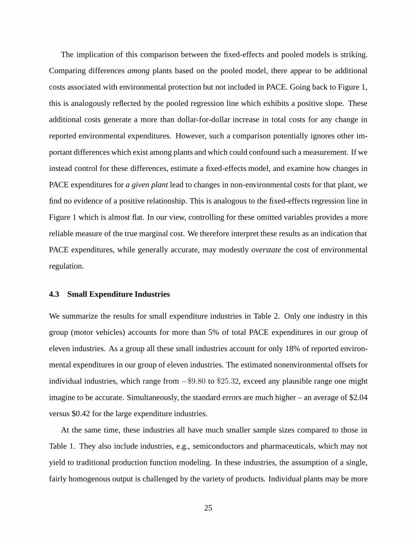
4.3 Small Expenditure Industries

We summarize the results for small expenditure industries in Table 2. Only one industry in this

group (motor vehicles) accounts for more than 5% of total PACE expenditures in our group of

eleven industries. As a group all these small industries account for only 18% of reported environ-

mental expenditures in our group of eleven industries. The estimated nonenvironmental offsets for

individual industries, which range from−$9.80 to $25.32, exceed any plausible range one might

imagine to be accurate. Simultaneously, the standard errors are much higher – an average of $2.04

versus $0.42 for the large expenditure industries.

At the same time, these industries all have much smaller sample sizes compared to those in

Table 1. They also include industries, e.g., semiconductors and pharmaceuticals, which may not

yield to traditional production function modeling. In these industries, the assumption of a single,

fairly homogenous output is challenged by the variety of products. Individual plants may be more

25

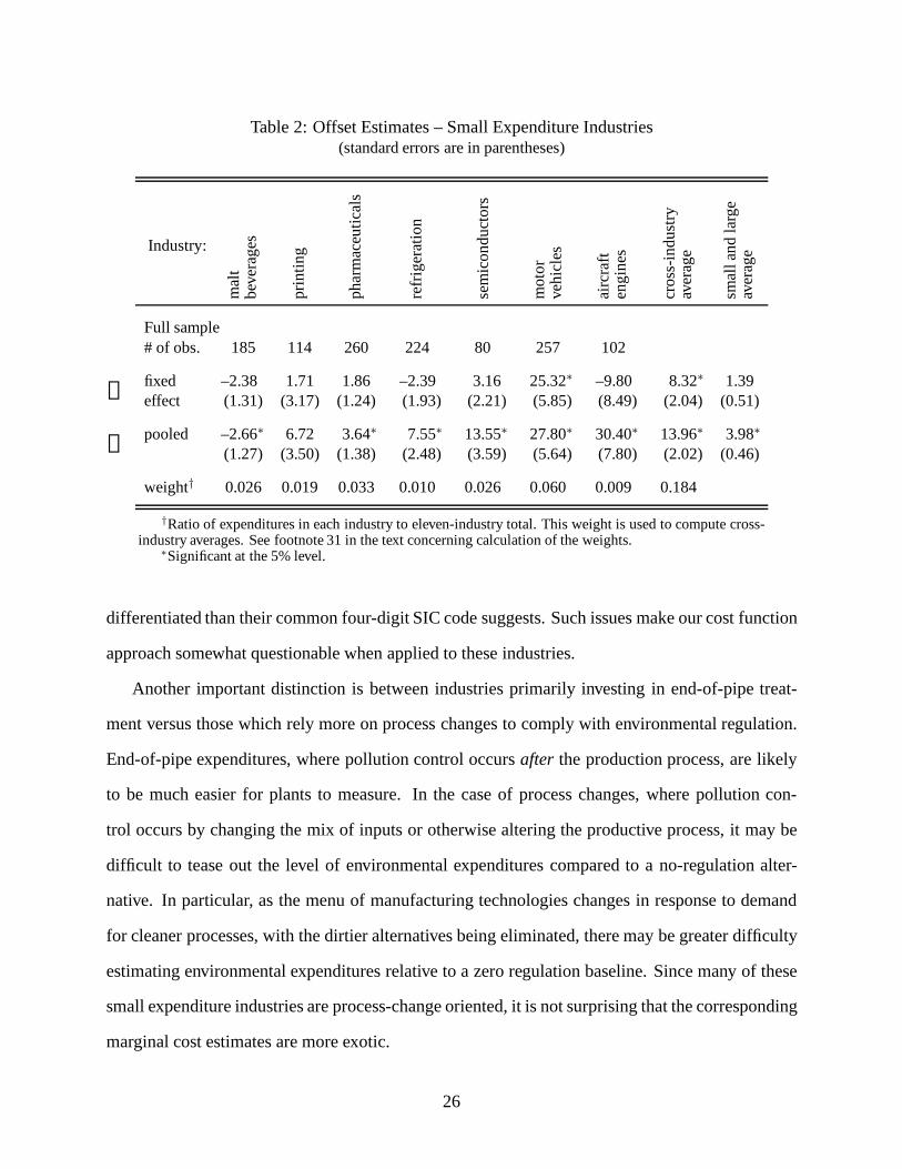
Table 2: Offset Estimates – Small Expenditure Industries(standard errors are in parentheses)

Industry:m

alt

bev

erag

es

prin

ting

ph

arm

aceu

tical

s

refr

iger

atio

n

sem

ico

nd

uct

ors

mo

tor

veh

icle

s

airc

raft

eng

ines

cro

ss-in

du

stry

aver

age

smal

lan

dla

rge

aver

age

Full sample# of obs. 185 114 260 224 80 257 102

➀fixed –2.38 1.71 1.86 –2.39 3.16 25.32∗ –9.80 8.32∗ 1.39effect (1.31) (3.17) (1.24) (1.93) (2.21) (5.85) (8.49) (2.04) (0.51)

➁pooled –2.66∗ 6.72 3.64∗ 7.55∗ 13.55∗ 27.80∗ 30.40∗ 13.96∗ 3.98∗

(1.27) (3.50) (1.38) (2.48) (3.59) (5.64) (7.80) (2.02) (0.46)

weight† 0.026 0.019 0.033 0.010 0.026 0.060 0.009 0.184

†Ratio of expenditures in each industry to eleven-industry total. This weight is used to compute cross-industry averages. See footnote 31 in the text concerning calculation of the weights.∗Significant at the 5% level.

differentiated than their common four-digit SIC code suggests. Such issues make our cost function

approach somewhat questionable when applied to these industries.

Another important distinction is between industries primarily investing in end-of-pipe treat-

ment versus those which rely more on process changes to comply with environmental regulation.

End-of-pipe expenditures, where pollution control occursafter the production process, are likely

to be much easier for plants to measure. In the case of process changes, where pollution con-

trol occurs by changing the mix of inputs or otherwise altering the productive process, it may be

difficult to tease out the level of environmental expenditures compared to a no-regulation alter-

native. In particular, as the menu of manufacturing technologies changes in response to demand

for cleaner processes, with the dirtier alternatives being eliminated, there may be greater difficulty

estimating environmental expenditures relative to a zero regulation baseline. Since many of these

small expenditure industries are process-change oriented, it is not surprising that the corresponding

marginal cost estimates are more exotic.

26

While it would have been reassuring to see results in the small expenditure industries parallel

those in the large expenditure industries, we find two useful messages in Table 2. First, some

patterns remain: the pooled estimates remain higher than the fixed-effects estimates for all but

one of the small expenditure industries (malt beverages), suggesting that omitted-variable bias

continues to be a problem. Second, the wide-ranging and implausible estimates may be just another

indicator of the poor quality of the underlying PACE data, only exacerbated by the small sample

size. This is consistent with the hypothesis that there may not be a systematic relationship between

reported environmental expenditures and additional economic costs/savings in some industries.

5 Conclusion

Most previous analyses find that reported environmental expenditures are likely tounderstatethe

true economic cost of environmental protection. In contrast, our results rule out any significant un-

derstatement and instead point to a modest though statistically insignificantoverstatement. Using

our preferred fixed-effects model, we estimate an aggregate savings of eighteen cents in conven-

tional production costs for every dollar of reported incremental pollution control expenditures with

a standard error of forty-two cents. This is equivalent to saying that a dollar increase in reported

environmental expenditures raises total (environmental + non-environmental) production costs by

eighty-two cents.

We observe economically large, though statistically insignificant, variation in our estimates

among industries. We find that reported environmental expenditures tend to generate savings in

conventional production costs in the petroleum refining, plastics, and pulp and paper industries. In

the iron and steel industry they generate added burdens. This variation could be viewed as a con-

sequence of acknowledged quality issues in the PACE data. Alternatively, the observed variation

might explain why some firms and/or industries may believe that PACE understates the true cost of

environmental protection even if, on average, PACE is roughly right or even overstates true costs.

An important finding in our work is that alternative assumptions about productivity differences

among plants produce vastly different estimates of economic costs. We find that estimates based

27

on an alternative, pooled model consistently show smaller savings and larger additional burdens

than the fixed-effects model. Use of a pooled model generates an aggregate estimate of $2.73 in

higher costs for every additional dollar of reported regulatory expenditure – versus $0.82 for the

fixed-effects model. In contrast to the fixed-effects specification, the pooled specification assumes

that unmodeled differences between plants (e.g., age, location, management style) are unrelated to

either total costs or reported environmental expenditures – or that environmental regulationcauses

those differences. Although the higher, pooled estimates are more consistent with previous work,

we believe they are biased by omitted variables characterizing differences among plants.

Previous work that found substantial understatement of regulatory costs has leaned on several

explanations of those results. Reduced flexibility, the crowding out of new investments, new source

bias or simply poor accounting are all plausible reasons why reported costs would understate actual

costs.

Our own observation of possible overstatement leans on two possible explanations: production

complementarities/economies of scope or, once again, poor accounting. A plausible complemen-

tarity story arises, for example, if shutting down a production line is a substantial expense. Then,

it makes sense that plant managers would undertake non-environmental modifications alongside

environmental ones in order to take advantage of the forced downtime. Since it is cheaper to do

the two modifications together rather than separately, this represents economies of scope. If the

cost of the downtime is entirely allocated to the environmental project, it would not be surprising

to find savings in conventional production associated with the increased expense on environmental

activities.

While we find no statistical evidence of either over- or understatement of the cost of environ-

mental regulation, the range of values included in a reasonable confidence interval, from 100%

overstatement to 70% understatement, is economically significant and deserves to be scrutinized

further. Based on these results, it is fair to say that the current emphasis on better measurement of

the benefits associated with environmental protection ought to be balanced with greater attention

to uncertainties about costs.

28

References

American Petroleum Institute (1996).Petroleum Industry Environmental Performance, FifthAnnual Report. Washington, DC: API.

Ashford, N. A., C. Ayers, and R. Stone (1985). Using regulation to change the market forinnovation.Harvard Environmental Law Review 9, 419–466.

Bailey, E. E. and A. F. Friedlaender (1982). Market structure and multiproduct industries.Jour-nal of Economic Literature 20, 1024–1048.

Barbera, A. J. and V. D. McConnell (1990). The impact of environmental regulation on in-dustry productivity: Direct and indirect effects.Journal of Environmental Economics andManagement 18, 50–65.

Bartelsman, E. J. and W. B. Gray (1994).NBER Productivity Database[online].URL:ftp://nber.nber.org/pub/productivity.

Bartik, T. J. (1988). The effects of environmental regulation on business location in the UnitedStates.Growth Change 19(3), 22–44.

Bartik, T. J. (1989). Small business start-ups in the United States: Estimates of the effects ofcharacteristics of states.Southern Economic Journal 55(4), 1004–1018.

Berndt, E. R. (1990).The Practice of Econometrics: Classic and Contemporary. New York:Addison-Wesley.

Caves, D. W., L. R. Christensen, and W. E. Diewert (1982a). The economic theory of index num-bers and the measurement of input, output, and productivity.Econometrica 50(6), 1393–1414.

Caves, D. W., L. R. Christensen, and W. E. Diewert (1982b). Multilateral comparisons of output,input and productivity using superlative index numbers.Economic Journal 92, 73–86.

Caves, D. W., L. R. Christensen, M. W. Tretheway, and R. J. Windle (1985). Network effectsand the measurement of returns to scale and density for U.S. railroads. In A. F. Daughety(Ed.),Analytical Studies in Transport Economics, pp. 97–120. Cambridge University Press.

Chamberlain, G. (1980). Analysis of covariance with qualitative data.Review of Economic Stud-ies 47, 225–238.

Chamberlain, G. (1984). Panel data. In Griliches and Intriligator (Eds.),Handbook of Econo-metrics, Volume 2, pp. 1247–1318. Amsterdam: North-Holland.

Christensen, L. and D. Jorgenson (1969). The measurement of U.S. real capital input, 1929-1967.Review of Income and Wealth, 293–320.

Cornwell, C. and P. Schmidt (1992). Models for which the mle and conditional mle coincide.Empirical Economics 17(1), 67–75.

Deily, M. E. and W. B. Gray (1991). Enforcement of pollution regulation in a declining industry.Journal of Environmental Economics and Management 21, 260–274.

Diewert, W. and T. Wales (1987). Flexible functional forms and global curvature conditions.Econometrica 55(1), 43–68.

29

Doniger, D. (1978).The Law and Policy of Toxic Substances Control: A Case Study of VinylChloride. Baltimore: Johns Hopkins University Press.

Engle, R. F., D. F. Hendry, and J.-F. Richard (1983). Exogeneity.Econometrica 51(2), 277–304.

Friedman, J., D. A. Gerlowski, and J. Silberman (1992). What attracts foreign multinationalcorporations? evidence from branch plant location in the United States.Journal of RegionalScience 32(4), 403–418.

Gray, W. B. (1987). The cost of regulation: OSHA, EPA and the productivity slowdown.Amer-ican Economic Review 77(5), 998–1006.

Gray, W. B. and R. J. Shadbegian (1994). Pollution abatement costs, regulation and plant-levelproductivity. Discussion Paper, U.S. Department of Commerce, Center for Economic Stud-ies.

Greene, W. H. (1990).Econometric Analysis. New York: MacMillan.

Griliches, Z. (1979). Sibling models and data in economics: Beginnings of a survey.Journal ofPolitical Economy 87(5, part 2), S37–S64.

Gruenspecht, H. K. (1982). Differentiated regulation: the case of auto emission standards.American Economic Review 72, 328–331.

Hall, R. and D. Jorgenson (1967). Tax policy and investment behavior.American EconomicReview 57, 391–414.

Hazilla, M. and R. J. Kopp (1986). The social cost of alternative ambient air quality standardsfor total suspended particulates: A general equilibrium analysis (final report). Technical re-port, Office of Air Quality, Planning and Standards, U.S. Environmental Protection Agency,Research Triangle Park, NC.

Hazilla, M. and R. J. Kopp (1990). Social cost of environmental quality regulation: A generalequilibrium analysis.Journal of Political Economy 98(4), 853–873.

Hsiao, C. (1986).Analysis of Panel Data. Cambridge: Cambridge University Press.

Hulten, C. R. and F. C. Wykoff (1981). The measurement of economic depreciation. In C. R.Hulten (Ed.),Depreciation, Inflation, and the Taxation of Income from Capital. Washington:Urban Institute Press.

Jaffee, A. B., S. R. Peterson, P. R. Portney, and R. N. Stavins (1995). Environmental regulationand the competitiveness of U.S. manufacturing: What does the evidence tell us?Journal ofEconomic Literature 33, 132–163.

Jorgenson, D. and R. Landau (1993).Tax Reform and the Cost of Capital: An InternationalComparison. Washington: Brookings.

Jorgenson, D. and K.-Y. Yun (1991).Tax Reform and the Cost of Capital. Oxford: ClaredonPress.

Jorgenson, D. W. and P. J. Wilcoxen (1990). Environmental regulation and U.S. economicgrowth.Rand Journal of Economics 21(2), 314–340.

Joshi, S., L. Lave, J.-S. Shih, and F. McMichael (1997). Impact of environmental regulations onthe U.S. steel industry. Mimeo, Carnegie Mellon University.

30

Leibenstein, H. (1966). Allocative efficiency vs. ‘X-efficiency’.American Economic Review 56,392–415.

Levinson, A. (1992). Environmental regulation and manufacturers’ location choices: Evidencefrom the census of manufactures. New York: Columbia University.

McConnell, V. D. and R. M. Schwab (1990). The impact of environmental regulation on industrylocation decisions: The motor vehicle industry.Land Economics 17(3), 67–81.

Meyer, S. M. (1993). Environmentalism and economic prosperity: Testing the environmentalimpact hypothesis. M.I.T. Mimeo, Cambridge, MA.

Mundlak, Y. (1978). On the pooling of time series and cross section data.Econometrica 46(1),69–85.

Nelson, R. A., T. Tietenberg, and M. R. Donihue (1993). Differential environmental regula-tion: Effects on electric utility capital turnover and emissions.Review of Economics andStatistics 77(2), 368–373.

Neyman, J. and E. Scott (1948). Consistent estimates based on partially consistent observations.Econometrica 16(1), 1–32.

Noreen, E. and N. Soderstrom (1994). Are overhead costs strictly proportional to activity? ev-idence from hospital service departments.Journal of Accounting and Economics 17, 255–278.

Palmer, K. L., W. E. Oates, and P. R. Portney (1995). Tightening environmental standards: Thebenefit-cost or the no-cost paradigm?Journal of Economic Perspectives 9(4), 119–132.

Palmer, K. L. and D. R. Simpson (1993). Environmental policy as industrial policy.Re-sources 10(4), 371–382.

Perroni, C. and T. F. Rutherford (1996). A comparison of the performance of flexible functionalforms for use in applied general equilibrium modelling. Mimeo, University of Colorado.

Porter, M. E. (1991, April). America’s green strategy.Scientific American.

Porter, M. E. and C. Van der Linde (1995). Toward a new conception of the environment-competitiveness relationship.Journal of Economic Perspectives 9(4).

Rose, A. (1983). Modeling the macroeconomic impact of air pollution abatement.Journal ofRegulatory Science 23(4), 441–459.

Schmalensee, R. (1993). The costs of environmental protection. InBalancing Economic Growthand Environmental Goods, pp. 53–80. Washington, DC: American Council for Capital For-mation.

Streitweiser, M. L. (1996). Evaluation and use of the pollution abatement costs and expendituresurvey. Mimeo, Center for Economic Studies, Bureau of Census.

U.S. Department of Commerce (various issues).Survey of Current Business.

U.S. Environmental Protection Agency (1990). Environmental investments: The cost of a cleanenvironment.

U.S. Office of Technology Assessment (1980). Technology and steel industry competitiveness.OTA-M-122, Washington, DC.

31

U.S. Office of Technology Assessment (1994). Industry, technology and the environment: Com-petitiveness, challenges, and business opportunities. OTA-ITE-586, Washington, DC.

Varian, H. R. (1992).Microeconomic Analysis(third ed.). New York: Norton.

A Data Sources

The data used in this paper are drawn from several plant-level datasets developed by the U.S.

Census Bureau:

• The Longitudinal Research Database (LRD). This is a pooled, cross-section, time seriescomprised of the establishment responses to the Annual Survey of Manufacture (ASM) andthe quinquennial Census of Manufactures (CM) for over 50,000 establishments in each year.The LRD contains information on cost, outputs and inputs at the plant level. Detailed quan-tity and expenditure information for energy consumption are only available up to 1981.

• The Manufacturing Energy Consumption Survey (MECS). Collected by the Department ofEnergy every three years beginning 1985, MECS contains detailed fuel consumption andexpenditure data by establishment.

• The Pollution Abatement Control Expenditure (PACE). This dataset includes pollution abate-ment investment spending and operating expenditures at the establishment level and has beencollected by the Census Bureau for most years between 1979 and 1991, except 1983 and1987.

For 11 four-digit SIC industries, our analysis includes the years 1979, 1980, 1981, 1985, 1988, and

1991. Sample sizes are shown in Table A.1.

Data on input and output quantities and prices are constructed as follows:

• Output.Data on the total value of shipments, by individual product codes, are contained inthe LRD. We construct a divisia index of output price based on the corresponding producerprices of different product obtained from Bureau of Labor Statistics (Caves, Christensen,and Diewert 1982a; Caves, Christensen, and Diewert 1982b). The quantity index is obtainedby dividing total value of shipments, adjusted for inventory, by this aggregate output priceindex.

• Regulation.Data on (nominal) annual pollution abatement operating costs at the plant levelare from the annual Pollution Abatement Costs and Expenditure (PACE) Survey. Operatingexpenses for pollution abatement include depreciation on the pollution abatement capital.Detailed data are available for the years 1979-1991, except 1983 and 1987. Real regulatoryexpenditures are computed by deflating nominal pollution abatement operating costs by theGDP deflator.

32

Table A.1: Sample Size by Industry

Industry Plants Sample Size

Malt Beverage 45 185Pulp and Paper 142 612Printing 45 114Plastic Material 107 403Pharmaceutical 73 257Petroleum 165 708Steel 127 527Refrigeration 76 224Semiconductors 28 80Motor Vehicles and Car Body 59 203Aircraft Engine 29 102

• Capital Stock.The gross book value of the capital stock at the beginning of the year and newcapital expenditures each year are reported in the LRD. Gross book value is used to computethe capital stock in 1979.34 A perpetual inventory method (Christensen and Jorgenson 1969)is then used to generate a real capital stock series covering the period 1980-1991 based onthe following formula:

kt = (1− δ)kt−1 +q0

qtIt (A.1)

wherekt is the periodt capital stock andIt is new capital expenditure measured in currentdollars. The industry-specific economic depreciation rate (δ) is from Hulten and Wykoff(1981). The capital stock price indices (qt) for various industries are drawn from a datasetdeveloped by Bartelsman and Gray (1994).

• Service Price of Capital.The service price of capital is calculated using the Hall-Jorgenson(1969) procedure. The service price of capital is given by:

pk(t) = [qt−1rt + δqt − (qt − qt−1) + qtCt]1− utzt − kt

1− ut(A.2)

where,

34Specifically, capital stock is initialized to 0.45 times the gross book value in 1979. This ratio is based on theaggregate net asset to gross book value ratio computed in the steel industry where firm 10-Ks were available.

33

pk(t) = service price of capital,qt = price index of new capital equipment,rt = after tax rate of return on capital (opportunity cost),δ = rate of economic depreciation,Ct = effective property tax rate,ut = effective corporate income tax rate,zt = present value of allowed depreciation tax deductions on a dollar’s

investment over the life time of an asset,kt = investment tax credit,t = year.

We use the average yield on Moody’s “Baa” bonds for the after tax rate of return on capital.The data on the tax policy variables are from Jorgenson and Yun (1991) and Jorgenson andLandau (1993).

• Capital Costs. The capital costs were constructed as the product of the service price ofcapital and the stock of capital.

• Labor. The quantity of labor is defined as the number of production workers. The cost oflabor includes production worker wages plus supplemental labor cost (which accured to bothproduction workers and non-production workers) adjusted to reflect the production workershare. The price of labor is defined as the cost of production workers divided by the numberof production workers.

• Price of Materials.Expenditure data on individual materials are collected on a five year cycleby the Census of Manufacturers (CM). We derive a divisia index of the price of materials foreach plant for the years 1977, 1982, 1987, 1992. Estimates for intervening years are linearlyinterpolated.

• Cost of Materials.We use reported total expenditures on materials and parts in the LRD tocalculate material costs.

• Price of Energy.Detailed data on total quantities consumed and total expenditures on variousfuels were collected in LRD (through 1981) and MECS (1985, 88, 91). These data are usedto calculate the prices of individual fuels ($/Mbtu) paid by each plant. The individual fuelsinclude coal, natural gas, dfo, rfo, lpg and electricity. These fuels typically account for about90 percent of total energy cost. The price of energy is computed as a divisia index of thesefuels.

• Cost of EnergyThe cost of energy is the summation of expenditures for the six individualfuels.

34

Table B.2: Estimation resultsa

(standard errors are in parentheses)

Sector:

mal

tb

ever

ages

pu

lpan

dp

aper

pri

ntin

g

pla

stic

s

ph

arm

aceu

tical

s

pet

role

um

stee

l

refr

iger

atio

n

sem

ico

nd

uct

ors

mo

tor

veh

icle

s

airc

raft

eng

ines

αy 0.7864∗ 0.7456∗ 0.7731∗ 0.8417∗ 0.4647∗ 0.6468∗ 0.7137∗ 0.7232∗ 0.4602∗ 0.7554∗ 0.7712∗(0.0293) (0.0278) (0.0679) (0.0356) (0.0462) (0.0383) (0.0300) (0.0252) (0.0927) (0.0214) (0.0463)

αr –0.0167 –0.0109 0.0073 –0.0150 0.0247 –0.0026 0.0112 –0.0119 0.0347 0.0675∗ –0.0257(0.0092) (0.0078) (0.0135) (0.0105) (0.0165) (0.0091) (0.0116) (0.0096) (0.0242) (0.0156) (0.0223)

αt –0.0097∗ 0.0109∗ 0.0286∗ 0.0124∗ 0.0383∗ –0.0033 –0.0023 0.0024 –0.0409∗ –0.0122∗ 0.0352∗(0.0019) (0.0011) (0.0030) (0.0020) (0.0034) (0.0020) (0.0022) (0.0025) (0.0123) (0.0024) (0.0045)

βkk 0.1020∗ 0.1047∗ 0.0425∗ 0.0501∗ 0.0660∗ 0.0101∗ 0.0693∗ 0.0067 0.0618 0.0033 0.0829∗(0.0155) (0.0172) (0.0126) (0.0119) (0.0112) (0.0018) (0.0073) (0.0049) (0.0937) (0.0036) (0.0191)

βll 0.0273 0.1055∗ 0.0842∗ 0.0684∗ 0.1423∗ 0.0141∗ 0.0572∗ 0.0744∗ 0.3072∗ 0.0274∗ 0.1709∗(0.0166) (0.0116) (0.0355) (0.0092) (0.0205) (0.0014) (0.0205) (0.0150) (0.0477) (0.0139) (0.0476)

βee 0.0180∗ 0.0693∗ 0.0093∗ –0.0140 0.0192∗ 0.0112∗ 0.0340 0.0084∗ 0.0279∗ 0.0009 0.0058∗(0.0034) (0.0073) (0.0038) (0.0146) (0.0078) (0.0018) (0.0182) (0.0014) (0.0081) (0.0006) (0.0029)

βyy –0.0678 –0.0215 0.2565∗ –0.0343 0.0603 0.0283 0.0432∗ –0.0292 0.1288∗ 0.1553∗ 0.0999∗(0.0388) (0.0322) (0.0980) (0.0335) (0.0460) (0.0236) (0.0198) (0.0223) (0.0476) (0.0248) (0.0200)

βtt –0.0012 0.0032∗ 0.0004 –0.0006 –0.0007 –0.0036∗ 0.0002 0.0041∗ –0.0034 –0.0105∗ –0.0056∗(0.0009) (0.0006) (0.0013) (0.0010) (0.0016) (0.0009) (0.0009) (0.0011) (0.0034) (0.0011) (0.0017)

βkl –0.0107 0.0053 0.0112 –0.0115 –0.0078 –0.0027∗ –0.0113 0.0168∗ –0.0323 –0.0132∗ –0.0285(0.0105) (0.0095) (0.0101) (0.0074) (0.0103) (0.0007) (0.0083) (0.0051) (0.0442) (0.0047) (0.0219)

βke –0.0012 –0.0229∗ 0.0009 0.0024 –0.0104 –0.0010 –0.0115 –0.0032∗ –0.0067 –0.0001 –0.0016(0.0034) (0.0080) (0.0048) (0.0077) (0.0067) (0.0011) (0.0064) (0.0014) (0.0119) (0.0005) (0.0043)

βky 0.0048 0.0056 0.0060 –0.0393∗ –0.0259∗ –0.0110∗ –0.0442∗ –0.0180∗ –0.0238 –0.0093∗ –0.0144∗(0.0072) (0.0070) (0.0066) (0.0047) (0.0068) (0.0021) (0.0030) (0.0019) (0.0177) (0.0012) (0.0064)

βkt 0.0004 0.0020∗ 0.0029∗ 0.0013∗ 0.0040∗ 0.0014∗ 0.0001 0.0021∗ 0.0497∗ 0.0023∗ 0.0012(0.0008) (0.0006) (0.0008) (0.0005) (0.0009) (0.0002) (0.0004) (0.0004) (0.0067) (0.0004) (0.0013)

βle 0.0072 –0.0159∗ 0.0027 –0.0079 –0.0068 0.0000 0.0220 –0.0052∗ –0.0218∗ –0.0013 –0.0078(0.0041) (0.0058) (0.0055) (0.0061) (0.0082) (0.0010) (0.0127) (0.0018) (0.0059) (0.0007) (0.0056)

βly –0.0031 –0.0477∗ –0.0294 –0.0299∗ –0.0731∗ –0.0051∗ 0.0032 –0.0146∗ –0.0450∗ –0.0340∗ –0.0432∗(0.0057) (0.0053) (0.0222) (0.0039) (0.0123) (0.0010) (0.0067) (0.0048) (0.0201) (0.0032) (0.0131)

βlt –0.0008 –0.0025∗ –0.0099∗ –0.0022∗ –0.0067∗ 0.0002∗ –0.0043∗ –0.0036∗ –0.0316∗ 0.0010 –0.0121∗(0.0007) (0.0005) (0.0023) (0.0005) (0.0014) (0.0001) (0.0010) (0.0008) (0.0061) (0.0009) (0.0024)

βey –0.0052∗ –0.0061 –0.0081∗ 0.0063 –0.0084 –0.0081∗ –0.0134 –0.0065∗ –0.0070∗ –0.0024∗ –0.0105∗(0.0014) (0.0052) (0.0034) (0.0088) (0.0051) (0.0015) (0.0080) (0.0006) (0.0033) (0.0002) (0.0015)

βet –0.0001 –0.0013∗ –0.0002 0.0012 0.0020∗ –0.0001 –0.0003 0.0002∗ 0.0028∗ 0.0002∗ 0.0000(0.0002) (0.0004) (0.0004) (0.0008) (0.0006) (0.0002) (0.0010) (0.0001) (0.0010) (0.0001) (0.0003)

βyt –0.0060∗ 0.0040∗ –0.0001 0.0113∗ 0.0124∗ –0.0020 –0.0002 –0.0031 –0.0045 –0.0146∗ 0.0106∗(0.0024) (0.0014) (0.0043) (0.0020) (0.0029) (0.0016) (0.0015) (0.0023) (0.0088) (0.0026) (0.0022)

35

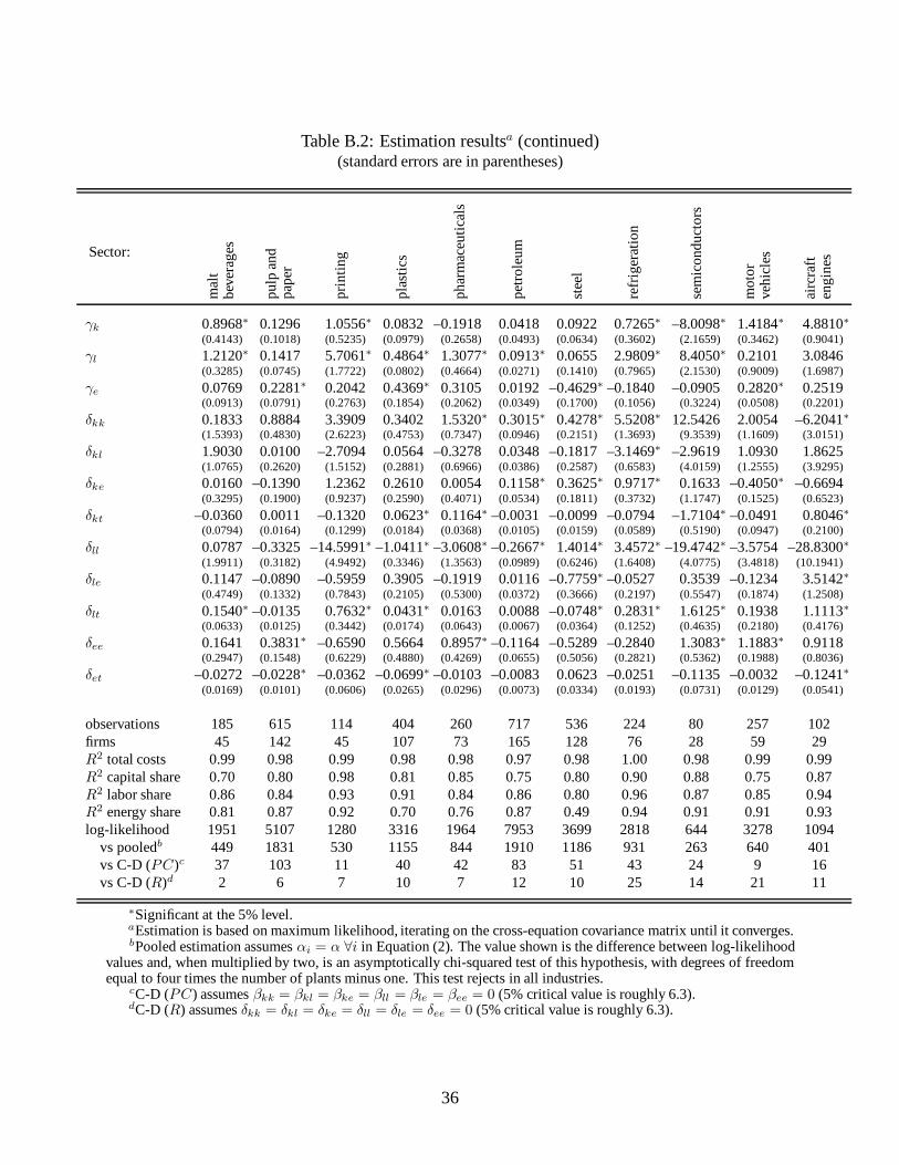
Table B.2: Estimation resultsa (continued)(standard errors are in parentheses)

Sector:

mal

tb

ever

ages

pu

lpan

dp

aper

pri

ntin

g

pla

stic

s

ph

arm

aceu

tical

s

pet

role

um

stee

l

refr

iger

atio

n

sem

ico

nd

uct

ors

mo

tor

veh

icle

s

airc

raft

eng

ines

γk 0.8968∗ 0.1296 1.0556∗ 0.0832 –0.1918 0.0418 0.0922 0.7265∗ –8.0098∗ 1.4184∗ 4.8810∗(0.4143) (0.1018) (0.5235) (0.0979) (0.2658) (0.0493) (0.0634) (0.3602) (2.1659) (0.3462) (0.9041)

γl 1.2120∗ 0.1417 5.7061∗ 0.4864∗ 1.3077∗ 0.0913∗ 0.0655 2.9809∗ 8.4050∗ 0.2101 3.0846(0.3285) (0.0745) (1.7722) (0.0802) (0.4664) (0.0271) (0.1410) (0.7965) (2.1530) (0.9009) (1.6987)

γe 0.0769 0.2281∗ 0.2042 0.4369∗ 0.3105 0.0192 –0.4629∗ –0.1840 –0.0905 0.2820∗ 0.2519(0.0913) (0.0791) (0.2763) (0.1854) (0.2062) (0.0349) (0.1700) (0.1056) (0.3224) (0.0508) (0.2201)

δkk 0.1833 0.8884 3.3909 0.3402 1.5320∗ 0.3015∗ 0.4278∗ 5.5208∗ 12.5426 2.0054 –6.2041∗(1.5393) (0.4830) (2.6223) (0.4753) (0.7347) (0.0946) (0.2151) (1.3693) (9.3539) (1.1609) (3.0151)

δkl 1.9030 0.0100 –2.7094 0.0564 –0.3278 0.0348 –0.1817 –3.1469∗ –2.9619 1.0930 1.8625(1.0765) (0.2620) (1.5152) (0.2881) (0.6966) (0.0386) (0.2587) (0.6583) (4.0159) (1.2555) (3.9295)

δke 0.0160 –0.1390 1.2362 0.2610 0.0054 0.1158∗ 0.3625∗ 0.9717∗ 0.1633 –0.4050∗ –0.6694(0.3295) (0.1900) (0.9237) (0.2590) (0.4071) (0.0534) (0.1811) (0.3732) (1.1747) (0.1525) (0.6523)

δkt –0.0360 0.0011 –0.1320 0.0623∗ 0.1164∗ –0.0031 –0.0099 –0.0794 –1.7104∗ –0.0491 0.8046∗(0.0794) (0.0164) (0.1299) (0.0184) (0.0368) (0.0105) (0.0159) (0.0589) (0.5190) (0.0947) (0.2100)

δll 0.0787 –0.3325 –14.5991∗ –1.0411∗ –3.0608∗ –0.2667∗ 1.4014∗ 3.4572∗ –19.4742∗ –3.5754 –28.8300∗(1.9911) (0.3182) (4.9492) (0.3346) (1.3563) (0.0989) (0.6246) (1.6408) (4.0775) (3.4818) (10.1941)

δle 0.1147 –0.0890 –0.5959 0.3905 –0.1919 0.0116 –0.7759∗ –0.0527 0.3539 –0.1234 3.5142∗(0.4749) (0.1332) (0.7843) (0.2105) (0.5300) (0.0372) (0.3666) (0.2197) (0.5547) (0.1874) (1.2508)

δlt 0.1540∗ –0.0135 0.7632∗ 0.0431∗ 0.0163 0.0088 –0.0748∗ 0.2831∗ 1.6125∗ 0.1938 1.1113∗(0.0633) (0.0125) (0.3442) (0.0174) (0.0643) (0.0067) (0.0364) (0.1252) (0.4635) (0.2180) (0.4176)

δee 0.1641 0.3831∗ –0.6590 0.5664 0.8957∗ –0.1164 –0.5289 –0.2840 1.3083∗ 1.1883∗ 0.9118(0.2947) (0.1548) (0.6229) (0.4880) (0.4269) (0.0655) (0.5056) (0.2821) (0.5362) (0.1988) (0.8036)

δet –0.0272 –0.0228∗ –0.0362 –0.0699∗ –0.0103 –0.0083 0.0623 –0.0251 –0.1135 –0.0032 –0.1241∗

(0.0169) (0.0101) (0.0606) (0.0265) (0.0296) (0.0073) (0.0334) (0.0193) (0.0731) (0.0129) (0.0541)

observations 185 615 114 404 260 717 536 224 80 257 102firms 45 142 45 107 73 165 128 76 28 59 29R2 total costs 0.99 0.98 0.99 0.98 0.98 0.97 0.98 1.00 0.98 0.99 0.99R2 capital share 0.70 0.80 0.98 0.81 0.85 0.75 0.80 0.90 0.88 0.75 0.87R2 labor share 0.86 0.84 0.93 0.91 0.84 0.86 0.80 0.96 0.87 0.85 0.94R2 energy share 0.81 0.87 0.92 0.70 0.76 0.87 0.49 0.94 0.91 0.91 0.93log-likelihood 1951 5107 1280 3316 1964 7953 3699 2818 644 3278 1094

vs pooledb 449 1831 530 1155 844 1910 1186 931 263 640 401vs C-D (PC)c 37 103 11 40 42 83 51 43 24 9 16vs C-D (R)d 2 6 7 10 7 12 10 25 14 21 11

∗Significant at the 5% level.aEstimation is based on maximum likelihood, iterating on the cross-equation covariance matrix until it converges.bPooled estimation assumesαi = α ∀i in Equation (2). The value shown is the difference between log-likelihood

values and, when multiplied by two, is an asymptotically chi-squared test of this hypothesis, with degrees of freedomequal to four times the number of plants minus one. This test rejects in all industries.

cC-D (PC) assumesβkk = βkl = βke = βll = βle = βee = 0 (5% critical value is roughly 6.3).dC-D (R) assumesδkk = δkl = δke = δll = δle = δee = 0 (5% critical value is roughly 6.3).

36

B Estimation

Table B.2 presents detailed estimation results for the eleven industries considered in this study

using the fixed-effects model discussed in Section 3.3. Parameter estimates for the 30 free slope

parameters in Equation (3), standard errors, goodness of fit and likelihood statistics are reported.

The difference in the log-likelihood relative to three alternative models is also provided.

Over half of the estimated parameters are significant at the 5% level. Many of the second order

price coefficients are among the significant parameter estimates, both for the conventional produc-

tion function (β) and the environmental abatement cost function (δ). It should not be surprising,

then, that the tests of unit elasticity of substitution are rejected twenty-one out of twenty-two times.

The test that the model reduces to a pooled form, where all the fixed effects are the same, is

also strongly rejected. In every industry the test difference in likelihoods is on the order of ten

times the number of firms, whereas the critical value is on the order of four times the number of

firms, divided by two.

These tests suggest that the flexible functional form being estimated cannot be reduced in a

substantial way without significantly reducing the model’s fit. The goodness of fit statistics indicate

that large fraction of the observed variation is captured by our model. Much of this, especially in

the share equations, is accounted for by the fixed effects.

Table B.3 provides additional information about the consistency of the estimated share values,

fitted share values and own-price demand elasticities in light of economic theory. We first compare

the observed cost shares to values found in both aggregate data (U.S. Department of Commerce)

and another microeconomic study (Hazilla and Kopp 1990). Our estimates generally fall between

the two estimates reflecting the fact that the historical scope of our data lies between the the more

recent aggregate data and the older Hazilla and Kopp study.

Next we examine whether the fitted cost shares (e.g., factor demands) are positive and whether

the own-price elasticities are negative.35 Only a few of the fitted cost shares turn out to be negative.

This typically occurs in those industries where one or more shares is near zero (petroleum, for

35This is less restrictive than the concavity required by economic theory but is simpler to verify.

37

example, where materials account for over 90% of costs). However, a large number of the own-

price elasticities are positive, especially capital. This means that the factor demand schedules are

locally upward sloping in many cases, contradicting economic theory.

A commonly acknowledged problem with the translog cost function is it’s inability to accu-

rately capture relatively inelastic factor demand (Perroni and Rutherford 1996). Because the elas-

ticity varies with the factor shares, an average own-price elasticity near zero will imply that many

of the locally evaluated elasticities will be positive. This is in fact what we observe.

By estimating an alternative Cobb-Douglas model, we verify that the observed positive own-

price elasticities do not have important consequences for our primary results. This model re-

stricts the factor demands by imposing an own-price elasticity of -1. This specification leads to

an aggregate36 estimate of the offset associated with environmental expenditures of 0.28, larger

but insignificantly different from the translog estimate of−0.18. Since the Cobb-Douglas restric-

tion is strongly rejected based on the log-likelihood test, we continue to focus our attention on the

unrestricted model.

B.1 Distinguishing Environmental and Non-Environmental Cost Shares

Our econometric model is novel in that we estimate a cost function associated solely with produc-

tion of conventional outputY alongside factor shares associated with the production of bothY and

abatement effort. We are unable to estimate a cost function associated with abatement because we

are unable to control for the scale of abatement, which is unobserved. Also, the raw data do not

allow us to distinguish between those factor inputs used for abatement and those used for conven-

tional production, making it impossible to estimate share equations associated solely with conven-

tional production. However, the model specified in (3) circumvents this problem, distinguishing

econometrically between factors used for environmental and non-environmental production.

To understand how environmental and non-environmental cost shares are identified, it is useful

36E.g., across the four large expenditure industries: pulp and paper, plastics, petroleum and steel.

38

Table B.3: Assessment of Model Consistency

Industry:

mal

tb

ever

ages

pu

lpan

dp

aper

pri

ntin

g

pla

stic

s

ph

arm

aceu

tical

s

pet

role

um

stee

l

refr

iger

atio

n

sem

ico

nd

uct

ors

mo

tor

veh

icle

s

airc

raft

eng

ines

Comparison of average value shares

capital 0.056 0.092 0.059 0.063 0.074 0.020 0.060 0.026 0.136 0.015 0.047labor 0.141 0.201 0.359 0.085 0.238 0.019 0.230 0.236 0.370 0.118 0.333energy 0.028 0.120 0.024 0.057 0.032 0.022 0.104 0.016 0.046 0.006 0.022

Tab

leB

.2es

timat

esa

material 0.774 0.587 0.558 0.794 0.657 0.939 0.606 0.723 0.448 0.861 0.598

capital 0.131 0.153 0.166 0.173 0.302 0.105 0.074 0.099 0.166 0.063 0.067labor 0.177 0.265 0.350 0.180 0.314 0.071 0.299 0.366 0.387 0.123 0.414energy 0.014 0.052 0.012 0.049 0.014 0.021 0.095 0.012 0.019 0.008 0.011

19

87

I-O

tab

lesb

material 0.678 0.530 0.471 0.598 0.370 0.803 0.532 0.523 0.428 0.805 0.508

capital 0.020 0.066 0.054 0.059 0.071 0.055 0.061 0.032 0.166 0.032 0.021labor 0.116 0.202 0.362 0.212 0.146 0.039 0.258 0.292 0.387 0.231 0.298energy 0.013 0.046 0.009 0.040 0.112 0.037 0.034 0.016 0.019 0.010 0.013

Haz

illa

and

Ko

ppc

material 0.852 0.685 0.574 0.689 0.672 0.870 0.647 0.660 0.428 0.727 0.668

Fraction of observations with negative estimated share values (zeros are omitted)d

capital 0.005 0.005 0.018 0.002 0.004 0.060 0.024 0.027 0.038 0.101 0.069labor 0.007 0.004 0.001 0.025energy 0.002 0.025 0.027 0.007material

Fraction of observations with positive own-price elasticities (zeros are omitted)d

capital 0.968 0.730 0.526 0.436 0.485 0.287 0.692 0.121 0.288 0.218 0.971labor 0.037 0.559 0.277 0.389 0.007 1.000 0.176energy 0.070 0.171 0.061 0.010 0.415 0.237 0.032 0.134 0.188 0.004 0.069material 0.184 0.130 0.035 0.077 0.200 0.138 0.054 0.013 1.000 0.137

aAverage of the observed share values in each industry.bEnergy, materials and value added expenditures are from the 1987 Benchmark Input-Output Tables, U.S. Depart-

ment of Commerce (April, 1994). Further breakdown of value added is based on a more detailed version of GrossProduct Originating data, U.S. Department of Commerce (August, 1996).

cFrom Hazilla and Kopp (1986).

39

to consider a simpler model where production costs are given by

PC = α0 + αk logPk + αl log Pl + αe logPe + αm logPm

and the aggregate shares by

vk =R

R + PCγk +

PC

R + PCαk

etc. Here, the translog specifications have been simplified to Cobb-Douglas and all plant, time and

scale effects have been suppressed. The share equations can be rewritten

vk = αk +R

R + PC(γk − αk) (B.3)

Based on (B.3) one way to view the distinction between cost shares is how variation in the level

of regulatory expenditures leads to different aggregate factor shares, all else equal. Suppose, for

example, that no abatement occurs andR/(R + PC) = 0. The observed cost share of capital

would then reveal the value ofαk, the underlying non-environmental cost share. In contrast, if no

production of conventional outputY occurs andR/(R + PC) = 1, the observed cost share of

capital would reveal the value ofγk, the underlying environmental cost share. While we are un-

likely to observe such extreme cases, variation inR/(R+PC) coupled with our specific modeling

assumptions are sufficient to distinguish environmental from non-environmental factor inputs.

If the ratio of regulatory expenditures to total costs,RR+PC

is constant, this method of identi-

fication will not work.37 That is, if RR+PC

is constant, it becomes colinear with the constant term

in (B.3). However, jointly estimating the production cost model with the share equations contin-

ues to identify all the parameters even in this case. Specifically, theα’s will be identified by the

cost/price elasticities in the cost function and theγ’s will be identified by the difference betweeen

those cost/price elasticities and the observed aggregate share values. In other words, as input prices

vary, changes in non-environmental production costsPC identify theα parameters. Descrepancies

between these values and the observed cost shares then reveal theγ parameter values.

The standard motivation for estimating the share equations jointly with the cost function is to

improve efficiency by providing multiple relations (cost function and share equations) that involve37In the petroleum sector, this ratio varies from less than 0.01% to slightly more than 11.0% with a mean of 1.1%

and standard deviation of 1.2%.

40

only those parameters in the original cost function. Under the aforementioned circumstances,

however, this gain is nullified by the additional parameters that appear in the share equations (γ’s).

It is therefore possible that this effort to estimate multiple equations will be no more efficient

than the estimation of a single cost function equation. These circumstances require (a) a lack of

variation inR/(R + PC), the share of reported regulatory expenditures in total costs, and (b)

additional parametersγ that appear one-for-one with eachα appearing in the share equations.38

To the extent that these conditions arenotsatisfied, there continue to be efficiency gains from joint

estimation.

B.2 Parameter Validity

Since our goal is to use the estimated parameters to compute the cost of environmental expendi-

tures, the validity of these parameter estimates is critical.39 Our estimates hinge on the following

key assumptions:

1. The translog cost function given in Equation (2) provides a reasonable local approximation

to the true underlying cost function.

2. The data are measured accurately.

3. Input prices and the level of output are fixed prior to the plant’s production decisions each

period.

There are, of course, grounds to question each of these assumptions. The first assumption deals

with specification: if the model is misspecified, the parameter estimates will be biased. More to

the point, the parameters are no longer structural in the sense of revealing the true nature of a

production technology. However, this is a criticism with little practical import since our model is

more flexible than other models which have been applied to the same problem. For the industries

with smaller samples discussed in Section 4.3, one might argue that our specification istooflexible.38If, for example, the model forPC were translog and the model for environmental costs were Cobb-Douglas, the

number of additional parametersγ would be smaller than the number of original parametersα, reducing this effect.39The consistency of the estimated parameters with economic theory, e.g., positive and downward sloping factor

demand, is explored in Table B.3 and discussed in the Appendix.

41

The second assumption raises the issue of measurement error in the data – a problem widely

acknowledged with regard to PACE data. However, since we want to relate reported expenditures to

actual costs, whether or not reported expenditures accurately reflect some well-defined cost concept

is not particularly important. Our concern that reported expenditures might be a poor indicator of

related changes in production costs actuallyhingeson the presence of some measurement error.

To the extent that this measurement error might be exacerbated by our fixed-effects approach – an

issue often cited in discussions of panel data (Griliches 1979) – there are several countervailing

points.40 The first is that the exacerbation of measurement error bias in fixed-effects estimates

hinges on the assumption that the measurement error is less correlated across observations from the

same plant than the underlying regressor (true regulatory expenditures). If instead the measurement

error is more correlated – as might arise if variation in plant accounting is the major source of error

– a fixed-effects modelremovesmeasurement error.41 Second, even if there is a bias, it is unclear

which direction it goes. With both positive and negative estimates of non-environmental offsets,

a bias towards zero has ambiguous results in the aggregate. Finally and most importantly, any

concern about measurement error must be balanced against the possibility of omitted variable bias.

Given the long list of potential confounding variables which could affect both reported regulatory

expenditures and total costs, the risk of falsely attributing such effects to reported expenditures

leads us to side strongly with the fixed-effects model.

The last assumption deals with the issue of endogeneity. Specifically, we are interested in

the effect of increased environmental expenditures – presummably caused by tighter regulations –

on non-environmental expenditures. If changes in non-environmental expenditures instead affect

environmental expenditures, or if some omitted variable besides regulation affects both, the esti-

40Measurement error in a given variable biases that coefficient estimate towards zero. See Section 9.5 of Greene(1990) regarding the general issue of bias due to measurement error and Chamberlain (1984) or Hsiao (1986) regardingthe issue of measurement error in panel data.

41Gray and Shadbegian (1994) make exactly the opposite point: if measurement error has nothing to do withdifferences between plants, using a fixed-effects model will serve only to remove a large fraction of the real underlyingvariation in data, e.g., between plants. This leaves measurement error as a larger percentage of the remaining within-plant variation. Such an effect would tend to favor the random-effects or pooled models, where between plant variationis preserved. We see no reason, however, to believe that measurement error is less related to plant differences than thetrue variation.

42

mated parameters may be biased.42 For example, suppose that downtime is a significant expense

and that plants have a number of planned production upgrades which remain unimplemented be-

cause of these downtime costs. When it becomes necessary to stop production to install additional

abatement equipment, these queued projects might be then simultaneously undertaken. This “har-

vesting” of non-environmental projects introduces a negative correlation between between envi-

ronmental expenditures and annual production costs – especially if the full cost of the downtime

is attributed to environmental expenditures and the non-environmental projects are productivity

enhancing.

Whether such a decrease in production costs is attributable to increased environmental ex-

penditures depends on whether the non-environmental improvements would, in fact, have been

implemented anyway. If so, we would have to view increased environmental expenditures as an

endogenous outcome of the decision to shut down production (made by the plant), rather than

an exogenous consequence of tighter regulation (made by some external authority). Deily and

Gray (1991) have gone even further, arguing that the level of external regulatory stringency and

enforcement is itself sensitive to productivity shocks (e.g., production costs), potentially making

environmental expenditures endogenous even if they are beyond the control of the plant.

There is no easy way to deal with this potential endogeneity. On the one hand, there has

been considerable exogenous variation over time in regulatory stringency.43 This only indirectly

addresses the issue, however, by suggesting the endogenous response is likely to be small. On

the other hand, instrumental variables which might be used to isolate only exogenous changes in

regulation are likely to vary only across plants.44 As pointed out in Section 3.3, using variation

across plants to estimate the effect of regulation is itself problematic because of omitted plant-

specific variables. It is our belief that omitted-variables bias is the more significant of these two

42In particular, we need environmental expenditures to bepredetermined(see Engle, Hendry, and Richard 1983).43The level of stringency of air, water, and waste regulations increased significantly over the period of our data

(1979-91). In (real) dollar terms, total environmental expenditures (with investment outlays annualized at a 7% dis-count rate) have doubled over the period (U.S. Environmental Protection Agency 1990) while reported annual PACEexpenditures have increased by 50%.

44For example, the instruments used by Gray and Shadbegian (1994) – activeness of state enforcement, fuel use,inclusion in a non-attainment area – are all primarily, if not exclusively, plant-specific characteristics.

43

problems.45 In Section 4.2 we see that this omitted-variable bias is potentially quite large.

45Gray and Shadbegian (1994) test the exogeneity of regulatory expenditures with respect to output and fail to rejectthat hypothesis. The relevance of the their test to our predicament is unclear, however, since they are using a differentdependent variable and are focused on cross-section variation, which we ignore.

44