THE COST OF CAPITAL UNDER DIVIDEND IMPUTATION

Prepared for the

AUSTRALIAN COMPETITION AND CONSUMER COMMISSION

by

Martin Lally

Associate Professor

School of Economics and Finance

Victoria University of Wellington

June 2002

The helpful comments of Jeff Balchin, David Chapman and other staff of the ACCCand the ORG (Victoria) are gratefully acknowledged. However, the opinionsexpressed here are those of the author.

2

EXECUTIVE SUMMARY 3

1. Introduction 5

2. The Officer Model 6

3. The Relevance of Foreign Investors 9

4. Estimation of the Utilisation Rate 12

5. Estimation of the Ratio of Imputation Credits to Tax Paid 18

6. Estimation of the Market Risk Premium 20

6.1 Estimation by Historical Averaging 20

6.2 Other Estimates From Historical Data 27

6.3 Forward-Looking Estimates 29

6.4 Summary 34

7. Differential Taxation of Ordinary Income and Capital Gains 34

7.1 Modeling Differential Taxation 34

7.2 Comparison of Models 37

7.3 Summary 40

8. Conclusion 42

REFERENCES 44

3

EXECUTIVE SUMMARY

In Australia a consensus seems to have developed in recent years in favour of the

“Officer” approach to valuation and cost of capital in the presence of Dividend

Imputation. This treats imputation as a process that lowers the company tax rate and

redefines dividends to include the attached imputation credits, to the extent that they

can be used. Furthermore, a consensus has also developed in favour of a 50%

reduction in the company tax rate, to reflect the benefits of imputation, and also in

favour of an estimated market risk premium of 6%. In its recent regulatory decisions,

in which output prices are prescribed for various firms, the ACCC has also favoured

this approach and these parameter estimates. It has also assumed that investors in

Australian companies are Australians rather than foreigners.

This paper has reviewed these conclusions, by addressing the following questions.

First, to what extent if any should foreign investors be recognized. Second, what is an

appropriate adjustment to the company tax rate to reflect the benefits of imputation.

This adjustment reflects both the utilization rate for imputation credits and the ratio of

credits assigned to company tax paid. Third, what is an appropriate estimate for the

market risk premium in the “Officer” model. Finally, and in view of the simplifying

assumption in the “Officer” approach that ordinary income and capital gains are

equally taxed, should an allowance be made for differential taxation of ordinary

income and capital gains.

The conclusions are as follows. First, regarding the issue of recognizing foreign

investors, continued use of a version of the Capital Asset Pricing Model that assumes

that national equity markets are segmented rather than integrated (such as the Officer

model) is recommended. It follows that foreign investors must be completely

disregarded. Consistent with the disregarding of foreign investors, most investors

recognized by the model would then be able to fully utilize imputation credits.

Second, regarding the appropriate adjustment to the company tax rate to reflect the

benefits of imputation, the utilization rate for imputation credits should be set at one,

and this follows from the first point above. In addition the ratio of imputation credits

assigned to company tax paid should be set at the relevant industry average, which

4

appears to be at or close to one for most industries. These two recommendations

imply an imputation-adjusted company tax rate of zero rather than the generally

accepted figure of 50% of the statutory rate. Put another way, they imply that the

product of the utilization rate and the ratio of imputation credits assigned to company

tax paid (denoted gamma by the ACCC) should be at or close to 1 for most companies

rather than the currently employed figure of 0.50. The effect of this change would be

to reduce the allowed output prices of regulated firms.

Third, in respect of the market risk premium in the Officer model, the range of

methodologies examined give rise to a wide range of possible estimates for the market

risk premium and these estimates embrace the current value of 6%. Accordingly,

continued use of the 6% estimate is recommended.

Finally, regarding the differential taxation of capital gains and ordinary income, the

simplifying assumption in the “Officer” model that they are equally taxed at the

personal level could lead to an error in the estimated cost of equity of up to 1.1%,

depending upon the relevant industry average cash dividend yield and franking ratio.

Prima facie this is a sufficiently large sum to justify use of a cost of equity formula

that recognizes differential personal taxation of capital gains and ordinary income, and

such a formula is presented in this paper. However a consensus has not yet developed

amongst Australian academics and practitioners for making such an adjustment and it

seems inappropriate for the ACCC to lead in this area. Consequently the continued

use of the Officer model is recommended. If such an adjustment were made, it would

raise the allowed output prices of some firms. However the argument for raising the

utilisation rate on imputation credits is at least as strong, and the net effect of the two

changes is unlikely to significantly benefit any firm.

5

1. Introduction

Since the introduction of Dividend Imputation in Australia in 1987 there has been

considerable debate concerning its implications for valuation and the cost of capital.

Two approaches have been employed. The first treats imputation as a process that

lowers the personal tax rate on cash dividends (Ball and Bowers, 1986; Australian

Department of Treasury, 1991; Monkhouse, 1993). Paralleling this was UK and New

Zealand work (Ashton, 1989, 1991; Cliffe and Marsden, 1992; Lally, 1992). The

second approach treats imputation as a process that lowers the company tax rate and

redefines dividends to include the attached imputation credits (van Horne et al, 1990;

Hathaway and Dodd, 1993; Officer, 1994). In recent years a consensus seems to have

developed in Australia in favour of the second of these approaches. Consistent with

this, the ACCC has favoured this approach (generally called the “Officer” model) in

its recent regulatory decisions1.

Nevertheless, a number of fundamental questions arise from the use of this approach.

The first concerns foreign investors, and the extent to which they should be

recognized, with the ACCC currently ignoring them. The second question concerns

the appropriate value for “gamma” in the Officer model, and its implications for the

market risk premium and the effective tax rate. The ACCC currently favours a value

of .50, but there are arguments for both lower and higher values. The third question

concerns the appropriate value for the market risk premium in the Officer model, with

the ACCC favouring a value of .06 but with arguments for alternative values. The

final question concerns the simplifying assumption within the Officer model that

ordinary income and capital gains are equally taxed. Clearly some investors face

lower tax on capital gains than on ordinary income, and this calls into question the

Officer assumption.

This paper seeks to address these four issues. Recent changes to the Australian tax

regime have implications for the usability of imputation credits and for the taxation of

capital gains, and the discussion will reflect this. The paper commences with a review

of the Officer model.

6

2. The Officer Model

Officer (1994) presents a model for the valuation of companies in the presence of

dividend imputation. The model treats imputation as a process in which some

company tax is a prepayment of shareholders’ personal taxation on dividends. The

level of company taxation that is treated in this way is the amount assigned as

imputation credits, to the extent that investors can use them. The company tax rate is

then reduced to reflect this, and dividends are defined to be the sum of cash paid and

the imputation credits, to the extent they can be used. Officer formalizes the model in

the context of a level perpetuity, and there is some ambiguity in definitions.

However, Monkhouse (1993, 1996) develops a model that admits any cash flow

profile and there is less ambiguity in definitions. Two versions are presented,

corresponding to each of the two approaches to imputation that were discussed earlier

(as a reduction in company tax rather than personal tax on dividends). In respect of

the former, Officer, approach the value of the company is

[ ]

{ }∑−+−+

−−= t

ede

ttet

TLkkL

QEYETYEV

)1(ˆ)1(1

)()()(0 (1)

where Yt is the firm’s year t cash flow before deductions for interest and tax, Qt are the

year t deductions from Yt to yield taxable income for an unlevered firm, L is the

leverage ratio, kd the cost of debt, and ek̂ the cost of equity with dividends defined to

include utilized imputation credits. The company tax rate Te is defined as

−=

TAXICUTT ce 1 (2)

where Tc is the statutory company tax rate, U a weighted average over investor

utilization rates for imputation credits (each investor’s rate can range from zero to 1),

IC are the imputation credits assigned by the company during a period and TAX is the

company tax paid during that period. Clearly the ratio IC/TAX can vary from year to

1 This is purely a matter of form rather than substance. Lally (2000b, p 10-11) demonstrates that thetwo approaches are equivalent.

7

year, and this is recognized by Monkhouse (1996). It may also be stochastic. In the

interests of simplicity it is treated here as non-random and equal across time. The cost

of equity, with returns defined to include imputation credits to the extent that they can

be used, is

[ ] efmfe RkRk β−+= ˆˆ (3)

where Rf is the riskfree rate, eβ the equity beta defined against the Australian market

index, and mk̂ the expected rate of return on the Australian market portfolio inclusive

of imputation credits to the extent they can be used. This is identical to the standard

version of the CAPM (Sharpe, 1964; Lintner, 1965; Mossin, 1966) except that the

returns in (3) include imputation credits. If the parameter mk̂ is expressed as the sum

of the conventional expected return (cash dividends and capital gains), plus the

imputation credits to the extent of being usable, then the last equation becomes

efm

mmmfe R

DIVIC

UDkRk β

−++=ˆ (4)

where Dm is the cash dividend yield on the market portfolio, and ICm/DIVm is the

franking ratio for the market portfolio (the ratio of credits attached to cash dividends

paid). In equations (3) and (4), the equity beta is defined over returns inclusive of

imputation credits. Nevertheless, estimates are generally obtained from returns that

do not include the imputation credits. This inconsistency is innocuous because the

inclusion or exclusion of dividends has no appreciable effect upon beta estimates

(Brailsford et al, 1997, Table 4, reveals the similarity in beta results from use of the

AOI price and accumulation). The same conclusion then extends to the issue of

including or excluding imputation credits from the definition of dividends.

Turning now to Officer’s (1994) presentation, he introduces the symbol γ (“gamma”),

and defines it (ibid, p. 8) such that it must correspond to the following product in (2)

TAXICU (5)

8

However, he later (ibid, p. 9) uses it in such a way that it must correspond to the

utilization rate U. Clearly, if the ratio IC/TAX is equal to 1, then the two uses of

“gamma” coincide, and this is consistent with Officer’s consideration of a level

perpetuity scenario. However, outside of a level perpetuity scenario, the ratio IC/TAX

may be less than 1, and some estimates of “gamma” clearly reflect this possibility.

Consequently the use of the term “gamma” to describe two phenomena is a recipe for

confusion. The ACCC clearly uses the term to refer to the product in equation (5)

rather than the utilization rate. However, at various points, various writers have

defined it in a way that corresponds to the utilization rate. Accordingly, to avoid any

confusion, this paper desists from use of the term “gamma”. Instead it refers to the

utilization rate and the ratio of imputation credits assigned to company tax paid.

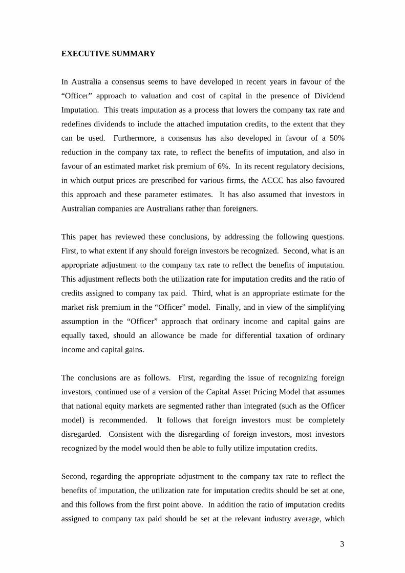
We now consider the valuation formula used by the ACCC (ACCC, 2000). This

matches equation (1), except that it values the cash flows to equityholders rather than

to equityholders and debtholders, i.e.,

[ ]∑+

−−−−=

te

tttett

kINTEQEYETBEYE

S)ˆ1(

)()()()()(0

where S0 is the value of the cash flows to equityholders, Bt is the year t payment to

debtholders (principal and interest) and INTt is the year t interest payment. The

allowed output price is then chosen (more precisely, an escalation rate applicable to a

base level of pricing is chosen) so that the present value of the cash flows to

equityholders equals the level of equity funding required (being proportion 1-L of the

investment required), i.e., the escalation rate in the output price is chosen so that

[ ]∑

+−−−−

=−t

te

tttett

kINTEQEYETBEYE

LA)ˆ1(

)()()()()()1( (6)

where A is the investment required.

9

3. The Relevance of Foreign Investors

Foreign investors are clearly significant in the Australian equity market, with around

30% of foreign shares so held (J.B. Were, 1996). Furthermore there is virtually free

flow of equity capital between Australia and the world’s principal equity markets.

Prima facie it then seems that models for valuation and the cost of capital should take

account of this. However modeling all features of the real world is impossible, and

certain abstractions are unavoidable. Inter alia, the Officer version of the CAPM (like

the standard version) assumes that national equity markets are completely segregated.

As a consequence the “market” portfolio is an Australian one, and betas are defined

against it. Versions of the CAPM have been developed that recognize that

international investment opportunities are open to investors, starting with Solnik

(1974). We will examine this model because, dividend imputation aside, it closely

parallels the Officer model. As with most international versions of the CAPM,

international capital flows are assumed to be unrestricted and investors exhibit no

irrational home country biases, i.e., there is no preference for local assets for non-

financial reasons. Like the standard version of the CAPM, it assumes that interest,

dividends and capital gains are equally taxed. The resulting cost of equity for an

Australian company is2

ewwfe MRPRk β+= (7)

where Rf is (as before) the Australian riskfree rate, MRPw is the risk premium on the

world market portfolio and βew is the beta of the company’s equity against the world

market portfolio. By contrast with the Officer CAPM in equation (4), there is no

recognition of dividend imputation. However, since most investors in Australia’s

equity market would be foreigners in this full internationalization scenario, and

foreigners gain only slight benefits (at most) from imputation credits under any

imputation regime, this feature of the model is not significant. The remaining, and

significant, distinction between the models lies in the definition of the market

2 This cost of equity is defined in respect of returns that do not include imputation credits, and istherefore denoted as ke without the “hat”.

10

portfolio, i.e., the “market” is Australian in the Officer model and the world in the

Solnik model. Thus the market risk premiums may differ across the two models and

the beta of an asset is defined against a different portfolio.

These distinctions in the market risk premium and beta have significant numerical

implications. In respect of the market risk premium, under the Officer model, an

estimate of the Australian market risk premium is about .06 (this is discussed in

section 6). By contrast, under the Solnik model in which markets are assumed to be

integrated, investors will now be holding a world rather than a national portfolio of

equities, and the latter will have a considerably lower variance due to the

diversification effect. Since the market risk premium is a reward for bearing risk, then

the world market risk premium under integration should be less than that for Australia

under segmentation. Stulz (1995) argues that, if the ratio of the market risk premium

to variance is the same across countries under segmentation, the same ratio will hold

at the world level under integration and this fact should be invoked in estimating the

world market risk premium3. Merton (1980) estimates the ratio at 1.9 for the US for

the period 1926-78. Harvey (1991, Table VIII) offers estimates for 17 countries over

the period 1970-90, which average 2.3. All of this suggests a figure of about 2. If we

use this figure then this suggests a market risk premium for the Solnik CAPM of

22 wwMRP σ= (8)

Cavaglia et al (2000) estimates the world market variance over the period 1985-2000

as .1352. Substitution into equation (8) then implies an estimate for the world market

risk premium of about .04.

Turning now to the question of betas, the average Australian stock has a beta against

the Australian market portfolio of 1, by construction. Similarly, the average asset

world-wide has a beta against the world market portfolio of 1, but this does not imply

that the average Australian stock has a beta of 1 against the world market portfolio.

Ragunathan et al (2001, Table 1) provide beta estimates for a variety of Australian

3 It would not be sensible to attempt to estimate the world market risk premium by historical averaging overa long time-series of returns, because even if markets were currently fully integrated this would not havebeen true for very long.

11

portfolios for the period 1984-1992, against both Australian and world market

indexes. The average of the latter to the former is about .40. In addition Gray (2000)

regresses the Australian index against a world index, for the period 1995-2000, and

obtains a beta of .72. The fact that these estimates are less than 1 is unsurprising in

view of Australia’s small weight in the world market index and the large weights for

some markets. To illustrate this point, suppose the world comprised four equity

markets with weights of .01, .245, .245 and .50. Also, the correlation between all

markets is .30 (Odier and Solnik, 1993) and they have the same variance. It follows

that the small market (market 1) has a beta against the world portfolio of

55.)50.245.245.01(.

)50.245.245.01,.(

4321

432111 =

++++++

=RRRRVar

RRRRRCovwβ

regardless of the value for the common variance. The other three markets have betas

of .84, .84 and 1.16 (the weighted average of the four betas is of course 1). Lally

(1996, Appendix 2) presents a more realistic example utilizing actual country weights

but the outcome is similar: ceteris paribus, very small markets have betas against a

world market portfolio that are much less than 1. For illustrative purposes we will

assume a beta for a typical Australian stock against the world market portfolio of .70.

We now combine this information about betas and market risk premiums. Employing

the Officer CAPM in equation (4), a riskfree rate of .06, and the estimated market risk

premium of .06 referred to above, the cost of equity for an average Australian stock

would be

12.)1(06.06. =+=ek

By contrast, under the Solnik CAPM in equation (7), with the Australian riskfree rate

of .06, and estimates for the world market risk premium and the beta of an average

Australian stock against the world market portfolio as indicated above, the cost of

equity for an average Australian stock would be

088.)70(.04.06. =+=ek

12

The difference in costs of equity under the two models is quite substantial, and is

essentially due to the difference in the market portfolio. Since the difference is so

large, and the Officer model rests upon an assumption about segregation of national

equity markets that is clearly false, then the Solnik model (or some other international

CAPM) would appear to be more appealing. However the real test is which is the

better description of how the expected returns on equities are determined. All direct

tests of this question suffer from the Roll (1977) problem, in which the use of mere

proxies for the true market portfolio may induce significant test biases. However less

direct tests can be performed. One of these is to examine investors’ portfolios. The

Solnik model implies that all investors will hold risky assets (both foreign and local)

in proportion to their market values. Clearly this is not the case, with investors

exhibiting pronounced home country bias, i.e., investors in most major markets hold

at least 90% of their risky asset holdings in home country assets (Cooper and

Kaplanis, 1994; Tesar and Werner, 1995). Not all international versions of the CAPM

have the same implications for investor portfolio holdings, but none can be readily

reconciled with this overwhelming home country bias (Huberman, 2001).

In view of this significant difficulty, it is understandable that analysts in Australia and

elsewhere have not (yet) invoked international CAPMs in estimating the cost of equity

capital. Furthermore, until home country bias is significantly ameliorated, such

caution is likely to persist. A similar caution is warranted in setting the costs of

capital for regulated industries. Thus the continued use of a version of the CAPM that

assumes capital markets are completely segregated (such as the Officer model) is

recommended. Consistency then requires that foreign investors be completely

disregarded.

4. Estimation of the Utilisation Rate

The utilisation rate is a weighted average across the imputation utilisation rates of

investors. This is unclear in Officer (1994) but is clear from Monkhouse (1993).

Furthermore, and this is not clear in even Monkhouse, it is a weighted average over all

13

investors in the market rather than those holding the equity in a particular company4.

Consistent with this, the same utilisation rate arises inside the company’s effective tax

rate in equation (2) and in the market risk premium in equation (4). The fact that this

utilization rate is a weighted average across investors implies that it is not the rate for

the “marginal” investor.

One approach to estimating this parameter derives from the fact that the Officer model

(like the standard CAPM) assumes that national equity markets are segmented.

Consistency then suggests that U be estimated on the basis that all investors in

Australian equities are Australians. In respect of such investors, most of those who

are taxed can fully utilise the credits, whilst tax-exempt investors cannot5. Wood

(1997, footnote 10) estimates that the proportion of shares held by Australians who

are tax exempt is 3-4%. Thus the estimate of U should be very close to 1. Even this

estimate presumes that tax-exempt investors cannot sell the credits to those who can

use them. In so far as they can, the estimate of U should be even closer to 1.

An alternative, and more popular, approach to estimating U is to do so from

examination of ex-dividend day returns. Bruckner et al (1994), using data from 1990-

93, estimated U as 0.68. The mechanism was as follows: per $1 of cash dividend the

maximum imputation credit attachable with a corporate tax rate (Tc) of .39 was

64.39.1

39.1

=−

=− c

c

TT

In addition the average ex-dividend day price drop per $1 of cash dividends was $1.06

for fully franked dividends and 62c for unfranked ones, a difference of 44c. The

value U then satisfied the following equation:

44.0$)64.0($ =U (9)

4 In the work of Cliffe and Marden (1992), and Lally (1992), it is clear that the averaging is over allinvestors in the market place. This averaging is a consequence of aggregating over investors in order toobtain market equilibrium. In intuitive terms the explanation is that market prices are determined byinvestors in aggregate.5 Recent tax changes allow investors a tax rebate instead of a tax credit for the imputation credits, and thisshould allow most taxed investors to fully benefit from the imputation credits.

14

This implies that U = 0.68. Other studies yield a range of values: Hathaway and

Officer (1995) obtain U = 0.44 using 1986-95 data, Brown and Clarke (1993) obtain

0.80 using 1989-91 data6, and Walker and Partington (1999) obtain 0.88 using

contemporaneous cum and ex trades in 1995-97. Taking account of these studies, an

estimate for U of around .60 is generally employed7.

This approach to estimating U is subject to a number of problems. Firstly, the 95%

confidence intervals on the estimates are large (for example, Bruckner et al’s is from

.44 to .92). Secondly, ex-dividend day returns are known to exhibit perverse

behaviour, which contaminates the estimate (see, for example, Frank and Jagannathan,

1998, in respect of Hong Kong and Brown and Walter, 1986, in respect of Australia).

Thirdly, these studies assume that capital gains and ordinary income are equally taxed

in Australia. This is clearly not the case, and this issue will be examined in more

detail in section 7. If capital gains are taxed at 10%, and ordinary income at 30%,

then equation (9) becomes

)10.1(44.0$)30.1)(64.0($ −=−U

and this implies U equals 0.88 rather than 0.68.

Finally, these estimates of U may and presumably do reflect the presence of foreign

investors in the Australian market, who cannot use or fully use the credits and this

exerts a downward effect on the estimates8. However, as noted earlier, the Officer

CAPM (like the standard CAPM) assumes that national equity markets are segmented.

Consequently the use of an estimate for U that is potentially significantly influenced

by the presence of foreign investors introduces an inconsistency into the model. One

possible response to this might be to argue that the shortcoming from use of a model

that fails to reflect the reality of international capital flows should not be compounded

by using an estimate of U that also fails to reflect international investors. However

6 Brown and Clarke use slightly different methodology enabling them to include partly franked dividends inthe data set.7 Interestingly McDonald (2001) obtains a similar figure in a study of the German market.8 J.B. Were (1996) estimate that 30% of Australian equities were foreign owned. This fact alone wouldpoint to an estimate for U of .70, which is almost identical to the Bruckner et al (1994) estimate.

15

the effect of recognising foreign investors only in this one respect would be to lower

the perceived value of a firm (and hence raise the output price allowed by the ACCC).

By contrast, the overall effect of internationalization is likely to involve raising the

value of a firm (and hence lower the output price that should be allowed by the

ACCC), because the adverse effect upon the usability of imputation credits is likely to

be more than offset by the positive effects from a lower risk premium. Thus

recognition of foreigners only in the estimate of U would push the calculated value of

a firm further away rather than closer to the “correct” answer, i.e., it leads to a raising

in the output price allowed by the ACCC when the appropriate direction is a lowering.

To illustrate this point, consider a regulated firm that has just been set up, with no

debt, and with assets costing $100m and of indefinite life. The expected output is 1m

units per year and there are no operating costs. Letting the allowed output price be

denoted P, then the expected cash flow in year 1 before company tax is $Pm. Taxable

income is likewise and both are expected to grow at 3% pa indefinitely. Consistent

with the discussion in the next section, the ratio IC/TAX is assumed to be 1. If equity

markets are fully segmented then a utilization rate U of close to 1 will prevail, and we

assume 1. In addition the Officer version of the CAPM is employed. Consistent with

the example in the previous section, we use a riskfree rate of .06, a market risk

premium of .06, and an equity beta of 1, leading to a cost of equity of .12. Following

equation (2), the effective tax rate is

[ ] 0)1(1130. =−=eT (10)

Following equation (6), the output price P should be chosen so that the present value

of the cash flows to equityholders, discounted at the cost of equity of .12, equals the

asset cost of $100m, i.e.,

03.12.

)01($.....)12.1(

)03.1)(01($12.1

)01($100$ 2 −−=+−+−= PmPmPmm (11)

Solving this yields an output price of $9. By contrast, if national equity markets are

completely integrated, then the Officer CAPM should be replaced by an international

16

version. Following the discussion in the previous section, we invoke the Solnik

model and the estimate there for the cost of equity of this firm of .088. In addition a

value for U of zero is invoked. Recomputing the effective tax rate in (10) and then the

output price in (11), the results are

[ ] 30.)0(1130. =−=eT

03.088.

)30.1($.....)088.1(

)03.1)(30.1($088.1

)30.1($100$ 2 −−=+−+−= PmPmPmm

Solving the last equation yields an output price of $8.28. Thus the full effect of

internationalization is to reduce the appropriate output price. By contrast, if one

continues to use the Officer model but recognizes the effect of internationalization

upon the value of U, by reducing the estimate from 1 to the generally employed figure

of .60, then the last two equations become

[ ] 12.)60(.1130. =−=eT

03.12.

)12.1($.....)12.1(

)03.1)(12.1($12.1

)12.1($100$ 2 −−=+−+−= PmPmPmm

Solving the last equation then yields an output price of $10.23. Thus the full effect of

internationalization would be to reduce the allowed output price by 10%, whereas

recognizing only a reduction in U leads to the allowed output price rising by 14%.

Thus the common practice of recognizing the effect of foreign investors in the

estimate of U, but not also in the choice of CAPM, has a totally perverse effect.

Accordingly it is not recommended.

In summary then, the estimate for U of around .60 that has been deduced from ex-

dividend studies is not recommended. Lonergan (2001) goes even further and argues

that an appropriate estimate of U is close to zero, primarily because Australia “..is a

price-taker in the world’s capital market”. He goes on to note that use of a higher

value for U by regulatory authorities leads to the result that “..some investors are

17

being deprived of part of the return to which they properly should be entitled”.

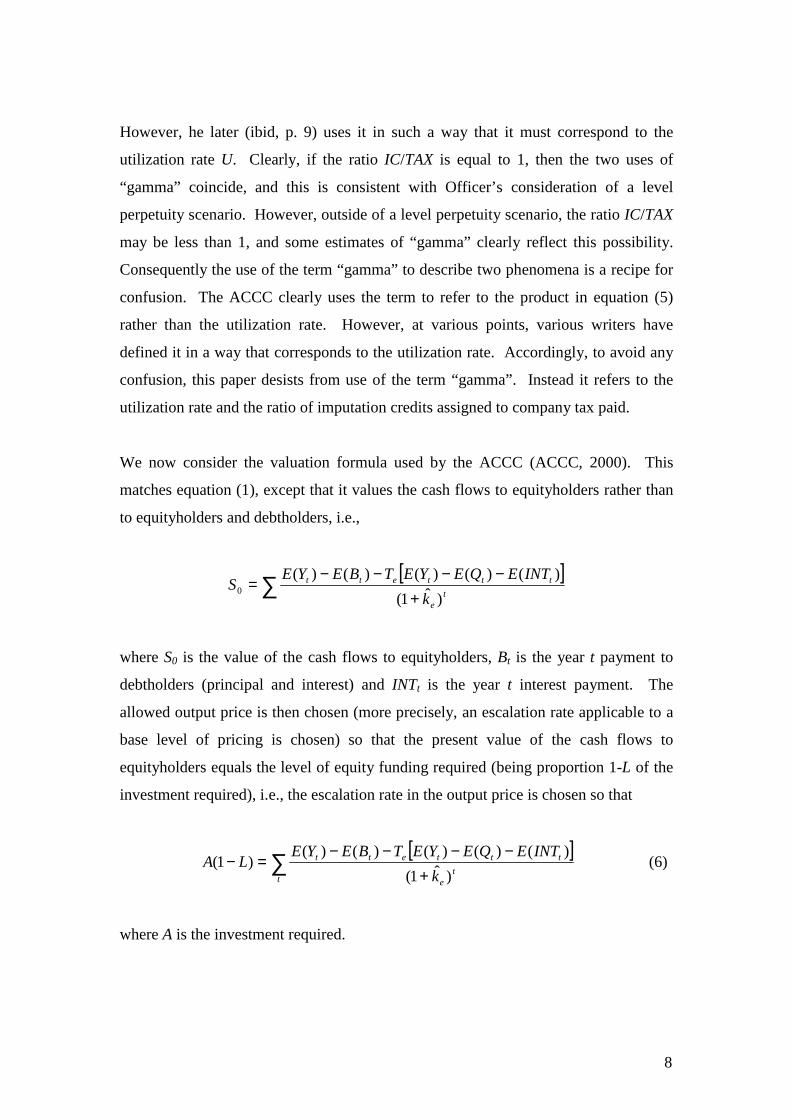
However, if it is true that Australia is a price-taker in the world’s capital market, then

it follows not only that the value of U is close to zero but also that the appropriate

CAPM to employ is an international version. In the above example, the allowed

output price should then fall from $9 to $8.28. However, if a value for U of zero was

adopted, but the Officer model was still used, then equations (10) and (11) would

become

[ ] 30.)0(1130. =−=eT

03.12.

)30.1($.....)12.1(

)03.1)(30.1($12.1

)30.1($100$ 2 −−=+−+−= PmPmPmm

Solving the last equation yields an output price of $12.86. However the correct figure

is somewhere between $8.28 and $9. By lowering the utilization rate U, but not also

modifying the form of the CAPM, a form of “cherry picking” is being practiced,

whose effect is to raise the allowed output price when it should be lowered.

An alternative means of illustrating the same point is to examine a recent ACCC

Decision in which a WACC is presented that includes within it the imputation effect

on company tax. Considering the Moomba Final Decision (ACCC, 2001), Table 2.14

presents a pre-tax nominal WACC of this form and the figure given is .0949. Inter alia

this calculation embodies a market risk premium of .06, an equity beta of 1.16 and a

“gamma” value of .50 (this is the product of U and the IC/TAX ratio). If gamma is

reduced to zero, as suggested by Lonergan, then the WACC will rise from .094 to

.097, i.e., in the direction recommended by Lonergan. However, consistency requires

that an international CAPM is also invoked. Using the Solnik model, with a market

risk premium of .04 and an equity beta reduced by 30% (as discussed earlier in section

4), the resulting WACC falls to .081, i.e., in the opposite direction to that

recommended by Lonergan10.

9 The formula here is Officer’s (1994) formula (7) converted to pre-tax terms by dividing throughWACC by (1-T).10 Lally (1998) considers this issue in the context of a CAPM that impounds the imputation tax effectinto the discount rate rather than the cash flows. The overall effect of a shift from a domestic to aninternational CAPM is to reduce the discount rate, and this implies a reduction in the allowed outputprice. This is consistent with the result obtained here.

18

In summary then, within the context of the Officer model, it is not appropriate to

recognize foreign investors. Consequently an estimate for the utilisation rate of close

to 1 is recommended.

5. Estimation of the Ratio of Imputation Credits to Company Tax Paid

Within the context of the Officer model, the ratio IC/TAX is firm specific. Variation

across firms will arise from variation in the ratio of Australian company tax paid to

Australian sourced “profits”, and variation in the ratio of cash dividends to “profits”11.

For example, a firm might generate “profits” of $4m, pay Australian company tax of

$1m and pay a dividend of $3m. There is no rationale for withholding imputation

credits, and hence this firm would be expected to attach the entire $1m as imputation

credits. The value of IC/TAX would then be 1, as would the payout rate. However,

the two rates can diverge. If the dividend (DIV) was less than $2.33m, the attached

imputation credits would have to be less than $1m, in accordance with the restriction

that

DIVDIVT

TDIVIC

c

c 43.30.1

30.1

=

−=

−

≤

Thus, if the dividend was $2m, then IC could not exceed $.86m. Assuming it was set

at this upper limit, then IC/TAX would be .86, and the payout rate would be .67. If the

dividend was $2.5m then IC/TAX would be 1 but the payout rate would be .83. These

examples demonstrate that the ratio IC/TAX may diverge from the payout rate, and

therefore the latter should not be treated as an estimate of the former. This caveat

appears warranted in the light of frequent suggestions that appear to involve using the

payout rate in this way.

11 Profit is used here to mean some performance measure on which dividends are based rather than tomean taxable income. The obvious performance measure is accounting profit. Also, as indicatedearlier, the Officer formula presumes that the operation being valued is Australian, and therefore anycompany taxes paid are Australian, which give rise to imputation credits.

19

Within the present context, in which the ACCC prescribes an output price, there are

some difficulties in utilizing the firm’s actual ratio IC/TAX. First, it raises the

computational burden to the ACCC. Secondly, it generates a further area of

controversy in estimation. Finally, if the firm’s ratio is less than 1, then the firm will

be encouraged to raise its payout rate, and such behaviour may be value damaging

because the valuation model employed does not capture all aspects relevant to

dividend policy12. However these concerns can be mitigated by using the relevant

industry average. This compromise is then recommended.

Notwithstanding this recommendation, the market average is still of interest, as an

indicator of a typical outcome at the industry level. Accordingly the ratios for the

eight largest listed firms in Australia were examined, i.e., Telstra, News Corporation,

NAB, BHP, Rio Tinto, Westpac, Commonwealth Bank and ANZ. Collectively they

constitute almost 50% of listed equity in Australia. In all cases their most recent

financial statements reveal that the ratio IC/TAX was equal to one. In respect of

Telstra, News Corp and BHP, it is evident that the ratio is one from the fact that some

recent dividends have not been fully franked. In respect of the remaining companies,

recent dividends have all been fully franked. Nevertheless there are currently no

surplus imputation credits. Accordingly, all company taxes that have been paid have

been passed on as imputation credits. This selective sample suggests that the ratio

IC/TAX is close to one for most industries.

In summary then, it is recommended that the ratio IC/TAX for the firm of interest be

set at the industry average. In most cases this should be at or close to one. In

conjunction with the recommended estimate for the utilization rate of 1, this implies

that the product of these two parameters (called gamma by the ACCC) should be at or

close to 1 for most firms. Thus the imputation-adjusted company tax rate should be

zero for most firms rather than the currently employed estimate of 50% of the

statutory tax rate. The effect of this change would be to lower the allowed output

prices of regulated firms.

12 For example, one factor relevant to dividend policy is the extent to which capital gains are taxed lessonerously than ordinary income. However, to simplify, the Officer model assumes that they areequally taxed.

20

6. Estimating the Market Risk Premium

6.1 Estimation by Historical Averaging

As indicated in equation (4) the market risk premium in the Officer CAPM is defined

as

fm

mmm R

DIVIC

UDk −+ (12)

A number of approaches are available for estimating this parameter. The first

employs historical data, and averages over the ex post annual outcomes for a long

time series. The ex-post outcome for (12) in any year is

fm

mmm R

DIVIC

UDR −+ (13)

where Rm is the actual rate of return on the market portfolio over a period, comprising

only cash dividends and capital gains. For years prior to 1987, when dividend

imputation did not operate, the central term in (13) disappears and the ex-post value is

simply Rm – Rf. This process of averaging over ex-post outcomes follows Ibbotson

and Sinquefield (1976), who applied it to US market returns from 1926.

In applying the process there are four significant controversies. The first concerns

how much historical data is used. Use of older data risks sampling from periods in

which the market risk premium was different. Disregarding all but the most recent

data guarantees an impossibly large standard error on the estimate. Theory offers no

guidance as to the optimal trade-off.

The second controversy involves whether the time-series averaging should be

arithmetic or geometric. Proponents of the latter (minority) view include Copeland et

al. (1994, pp. 260-263) and Damodaran (1997, pp. 126-127), and the effect of using

such a process is to reduce the estimate of the Australian market risk premium by

almost .02 (Dimson et al, 2000, Table 5). Theoretical support for the geometric mean

is offered by Blume (1974), who argues that one should seek an estimator m̂ of the

21

expected return m which has the property that, over n future years, the estimator nm̂ is

unbiased with respect to nm . For n = 1, the arithmetic mean is an unbiased estimator

of m. However, for n > 1, Blume shows that the arithmetic mean is biased up and the

geometric mean biased down. Accordingly he proposes a weighted average of the

two.

Cooper (1996) extends this approach to argue that, for discounted cash flow purposes,

one should seek an estimator m̂ such that nm)ˆ/(1 is unbiased with respect to nm/1 .

Because of both the power and inverse transformations just described, an estimator m̂

that is unbiased with respect to m will not meet this test. Thus the arithmetic mean is

inappropriate. However Cooper offers no support for the geometric mean. The

appropriate estimator lies above the arithmetic mean, and hence even further from the

geometric mean (which is always below the arithmetic mean). Furthermore, for n <

20 years, the preferred estimator is close to the arithmetic mean. For n > 20 years, the

preferred estimator departs significantly from the arithmetic mean but the effect on

present value is small.

A third level of sophistication is to allow for the well-documented evidence of

negative autocorrelation in long-horizon returns (see Fama and French, 1988a;

Poterba and Summers, 1988). Indro and Lee (1997) show by simulation that negative

autocorrelation affects the biases in both arithmetic and geometric means.

Nevertheless, for n < 20 years, the effect is very small so that Cooper’s conclusion is

preserved, i.e. the arithmetic mean is a good approximation13.

The third significant controversy in this area concerns the choice of term for the

riskfree rate. In principle it should correspond to the investor horizon implicit within

the CAPM. However the model gives no guidance in determining this. Booth (1999)

examines the errors that can arise. For example, suppose that the Ibbotson averaging

is done over market return net of the yield on long-term government bonds, but the

investor horizon is short term. The short-term investor horizon implies that the

expected market return (km) is the sum of the short-term government stock rate (RfS)

13 Indro and Lee examine the effect of negative autocorrelation on estimates of nm rather than nm/1 .Clearly the latter is more appropriate for DCF purposes.

22

plus the market risk premium (u). In addition the short-term investor horizon implies

that the long-term government bond rate (RfL) is the sum of the short rate plus a risk

allowance (p). It follows that the market risk premium relative to long bonds is

[ ] [ ] pupRuRRk fSfSfLm −=+−+=−

Thus, if the current value of p exceeds the historical average then the current value of

the market risk premium relative to long bonds will be low. However the Ibbotson

averaging process engaged in will embody the historical average for p rather than the

current value, and will therefore be biased up. Booth (1999) shows that the systematic

risk of long-term bonds is particularly high at the present time, suggesting that p is

currently high. Consequently, if the investor horizon is short-term, and the Ibbotson

averaging process uses yields on long-term bonds, it will be biased up. In addition,

even if the current value for p equals the historical average, error will still arise for

stocks whose beta differs from 1. It might seem that the solution here is to define the

market risk premium relative to short bonds. However, the investor horizon may be

long term, and therefore we just swap one source of bias for another.

Applying the Ibbotson methodology, with arithmetic averaging and long-term bond

yields (10 yr), Dimson et al (2000, Table 2) estimates the Australian market risk

premium at .07, using data from 1900-200014. This data omits inclusion of the central

term in (12). However, since this term applies only since 1987, the omission exerts

only a minor effect on the average across the full 100 years of data. To see this, the

current value for the central term in (12) involves a value for U of 1, a market

dividend yield of .032 (data courtesy of JP Morgan), and a franking rate of .19 (data

also courtesy of JP Morgan). The product is .006. If it is attributed to each of the 13

years since the introduction of imputation, the effect upon the estimate of (12) is to

raise it by less than .00115. In addition to this data issue, the introduction of

14 The data are largely drawn from Officer (1989), who had earlier estimated the premium using datafrom 1882-1987. However it should be noted that Officer uses bond yields in his calculation whereasDimson et al use bond returns. The use of bond yields seems more in accord with the model and theeffect of using them would be to slightly raise the estimate for the market risk premium.

15 The average cash dividend yield of the “market” over the 13 year period was in fact slightly morethan the current figure of .032 (data courtesy of JP Morgan). However the average franking rate islikely to have been less than the current value because franking credits can only be obtained from

23

imputation in 1987 would have introduced a regime shift (downwards) in km.

However, as noted by Officer (1994, p. 10) this should be equal to the central term in

(12) so that (12) would have been invariant to the regime shift.

A variant on the Ibbotson approach arises from Siegel (1992), who observes that the

expected real return on equity appears to be stable over time. This suggests that km

should be estimated from the long-run average real return on equity and the current

forecast for inflation. The market risk premium then follows by deducting the current

value for the riskfree rate, and Siegel generates significantly different results for the

US from this approach relative to the Ibbotson approach. This approach is free of the

problem identified by Booth (1991), and described above. However it ignores the

presence of dividend imputation. Notwithstanding this point, modifications can be

made.

Applying this approach, the average real value of Rm is .091 (Dimson et al, 2000,

Table 2), and forecast medium term inflation is .025 (Australian Department of

Treasury, 2001)16. Invoking the Fisher relationship, the current estimate for km is then

.118. Deducting the current long-term bond yield of .062 (using 10 yr bonds to be

consistent with the Dimson data17) generates an estimate for the market risk premium

over long-term bonds of

056.062.118. =−=− fm Rk

However, as noted, km will have experienced a regime shift downwards with the

introduction of imputation, equal to the central term in (12), i.e., UDmICm/DIVm. This

regime shift will have had little effect upon the historical average but a more

pronounced effect upon the current value. Thus, to estimate the current value of km,

one should deduct the current value of the central term from the above estimate of

.118. This estimate for km should then be inserted into equation (12) to yield an

estimate for (12) of

company tax paid after the introduction of imputation; this has no appreciable effect today but wouldhave had a downward effect in the first few years following 1987. Thus even the figure of .001 may betoo high.16 The forecast is from October 2001 but is not expected to change when it is updated shortly.17 The figure represents an average of the daily rates over April and May reported on the ReserveBank’s website.

24

fm

mm

m

mm R

DIVIC

UDDIVIC

UD −+

−118.

Clearly the central terms here disappear and we are left with the same estimate of .056

appearing in the preceding equation. This estimate is close to the .06 figure currently

used by the ACCC.

Whichever period, definition of the riskfree rate and form of averaging is used, there

are a number of concerns with this historical averaging methodology. First, the true

market portfolio is a value weighting of all risky capital assets (those held for

investment purposes). The proxy used in the historical averaging approach is listed

equity at most. This represents only a small proportion of the actual market portfolio,

and the rest is not obviously similar in its risk characteristics18. The resulting

potential for bias is well recognised in empirical tests of the CAPM – see Roll (1977),

Kandel and Stambaugh (1987), Shanken (1987), and Roll and Ross (1994). In respect

of the cost of equity capital, Lally (1995) indicates the potential for serious bias,

through non-compensating biases in estimating both beta and the market risk

premium.

The second concern is that the 95% confidence intervals on these estimates are large

enough to admit substantial estimation error, even if the true value has not changed

over the estimation period. With a standard deviation of .20 per year (see Dimson et

al, 2000, Table 5), and 100 years of data, the resulting 95% confidence interval is ±

.04. Since the point estimate arising from the Dimson data is .07, the 95% confidence

interval ranges from .03 to .11. Relative to the debate over the correct value, these

intervals are huge.

The third concern is that the estimates may be biased in a number of ways even if the

true value has not changed over time. One of these is survivorship bias, in that

estimation is based on data drawn from markets that survived, and this implies a

sample average return in excess of the population parameter. The theoretical work of

18 Stambaugh (1982) estimates that equities represent only about 25% of the US market portfolio.

25

Brown et al. (1995) suggests that substantial bias may thereby arise. In addition

Jorion and Goetzmann (1999) survey a large set of markets, many of which have

failed at some point, and find that the results from Anglo-Saxon markets are unusually

high by about .03. However Dimson et al. (2000) identify a number of deficiencies in

this study and, upon correcting for this, find that the results for Anglo-Saxon markets

are not unusual. In particular the Australian result is close to the average. Another

possible source of bias, suggested by Siegel (1992), is that unexpected inflation over

the post WWII period has led to real returns on bonds (but not stocks) being

significantly less than expected, and this has led to MRP estimates being biased

upwards.

The fourth concern is bias arising from changes over time in the true value. Siegel

(1999) suggests that the costs of acquiring a well-diversified portfolio (via a mutual

fund) have fallen considerably in the past 20 years, and offers an estimate for the

resulting reduction in the US market risk premium of .015. Other factors affecting the

market risk premium, and which may have changed, are the “term premium”, risk

aversion, personal taxation, market risk and internationalisation. The “term premium”

is the issue raised by Booth (1999), as discussed earlier, and it afflicts only the

Ibbotson approach to historical averaging. In respect of risk aversion, a number of

papers (Keim and Stambaugh, 1986; Campbell, 1987; Fama and French, 1988a, 1989;

Schwert, 1990) indicate that a set of time-varying variables that could be regarded as

proxies for risk aversion have some power to explain changes in the market risk

premium19. However the statistical reliability of these relationships is weak.

In respect of personal taxation Gordon and Gould (1984) examine Canadian data for

1956-82, and found that the market risk premium net of personal tax averaged 4.9%

over that period. They then construct a time-series for the pre-tax counterpart (i.e. the

standard market risk premium) that would preserve the 4.9%. They find that it would

have to vary enormously, from .5% to 5%! Such variation has two sources: changes

in personal tax rates and changes in the riskfree rate. In respect of the latter, an

increase in the riskfree rate implies a less than equal increase is needed in the pre-tax

expected return on equities so as to preserve the market risk premium net of personal

26

tax, because equities are taxed less onerously. Thus the pre-tax market risk premium

falls in response to this rise in the riskfree rate.

In respect of market risk, changes can be measured with a high degree of accuracy,

and they have been substantial. Merton (1980, Table 4) presents US estimates over

successive four year periods from 1926 to 1978, and finds that the annuallised

standard deviation ranges from .45 during the Great Depression to .11 during the

1960s. Finally, in respect of internationalization, clearly there have been considerable

developments since 1970. As indicated in section 3, this should lower the Australian

market risk premium.

The fact that the market risk premium changes is aggravated by the fact that, as it

changes, it drives equity prices and hence historical average returns in the opposite

direction. Thus the bias is aggravated. For example, the apparent decline in market

volatility over the sample period implies that the current market risk premium is

below the historical average. Thus there is upward bias in the historical average

return even if the decline in volatility did not raise market prices. The fact that it did

raise prices implies that the historical average return is even more biased as an

estimator of the current market risk premium. To illustrate this point, suppose that the

market risk premium recently fell by .02, inducing a decline in km from .13 to .11 and

raising market prices such that the average market return over the estimation period

was raised by .01. Most past market returns would then be drawn from a distribution

with mean .13 rather than the current value of .11. Consequently there will be an

upward bias of almost .02 in estimating the current market risk premium from past

data. In addition, the very event in question here raises average market returns by .01,

and thereby imparts a further bias of .01. Thus the aggregate upward bias in

estimating the current market risk premium from historical data is .03.

In recognition of this problem some authors (Fama and French, 2002; Jagannathan et

al, 2000) have sought to estimate the standard market risk premium by historical

averaging methods that avoid averaging actual market returns. The standard market

risk premium is

19 These include business conditions, dividend yields and returns on low grade versus high-grade

27

fm Rk −

and km is the sum of the expected dividend yield and the expected capital gain. The

expected dividend yield can be estimated by the historical average dividend yield.

The expected capital gain comes from expected growth in dividends, which in turn

comes from expected growth in profits, and this in turn from expected growth in GDP.

Fama and French (2002) estimate the expected capital gain from the average growth

rate in dividends and also from the average growth rate in profits. Coupling these

estimates of expected capital gain with the average dividend yield yields an estimate

of km. Subtracting the average value of Rf then yields an estimate of the market risk

premium. Jagannathan et al (2000) undertake a similar analysis except that they

estimate the expected capital gain from the average growth rate in GDP. Applying

these approaches to the US market yields estimates of the standard market risk

premium of .026 - .043, considerably lower results than those obtained by historical

averaging of the Ibbotson type. Results from the application of this methodology to

Australian data are not yet available.

6.2 Other Estimates From Historical Data

The possibility that the market risk premium has changed over time has given rise to

estimation processes that attempt to model this. The seminal paper in this area is

Merton (1980), who suggests that the (standard) market risk premium is proportional

to volatility and attempts to model this relationship. Scruggs (1998) clarifies the

earlier controversy about the sign of the relationship (French et al., 1987, and Glosten

et al., 1993, reach opposite conclusions) and concludes that it is positive. However

the functional form of the relationship is not apparent. Friend and Blume (1975)

conclude that aggregate relative risk aversion is constant, and this implies that the

standard market risk premium is proportional to variance (see Chan et al., 1992).

Merton estimates this ratio of the standard market risk premium to market variance at

1.9, using US data over the period 1926-78. Harvey (1991, Table VIII) offers

estimates for 17 countries over the period 1970-1990, with a mean of 2.3 and a

corporate bonds.

28

standard error of .3020. All of this suggests a figure of around 2. If we use this figure,

and couple it with an estimate for the Australian market variance of .1832 (Cavaglio et

al, 2000, Table 1, using data from 1985-2000), the resulting estimate of the Australian

market risk premium is

( ) 067.183.2 2 =

This is an estimate of the standard market risk premium, i.e., km – Rf. If the data used

to estimate the reward to risk ratio (estimated at 2) were drawn from the Australian

market in the period since imputation was introduced, the estimate of .067 would

require addition of the central term in (12). This would raise the .067 figure by about

.013, as discussed in the previous section. If the data were drawn from the Australian

market prior to the introduction of imputation, no adjustment would be required

because the standard premium in the pre-imputation period should be equal to the

Officer premium in the post imputation period. However the data are drawn from a

variety of markets, some with imputation and some without. Even in markets with

imputation (such as Australia) the data is drawn largely from the pre-imputation

period. Thus the figure of .067 requires some adjustment, but by much less than .013.

This suggests an estimate for the market risk premium of about .07.

As a form of cross-check, application of this methodology to the US market, along

with the above reward to risk ratio of 2 and an estimate of the US market variance

over the same 1985-2000 period (of 2153. : see Cavaglia et al, 2000, Table 1), yields

an estimate for the US market risk premium of

047.)153(.2 2 =

This is remarkably consistent with Cornell’s (1999, Chapter 4) estimate of .045 by the

forward-looking approach or Welch’s (2001) result of .045 from survey evidence

(using long-term bond yields in both cases).

20 Harvey also gives an estimate for Australia of 1.1, but the standard error of .90 is so large that theestimate is quite unreliable.

29

This approach to estimating the market risk premium avoids most of the problems

associated with historical averaging. However both the estimated reward to risk ratio

and the estimated variance are subject to statistical uncertainty, particularly the

former. There is also doubt surrounding the choice of variance rather than standard

deviation as a measure of volatility. Merton (1980) estimates the ratio for each of

these approaches, and they can generate dramatically different estimates of the market

risk premium.

In addition, even if the market volatility estimate is accurate, the resulting estimate of

the market risk premium is only good for a future period matching that for which

current volatility will remain unchanged. Clearly the fact that it has changed in the

past implies that it will do so in the future. If it follows a random walk without drift,

this will not be a concern because today’s value will then be the best estimate for all

future years. However, as one might expect, the market risk premium appears to

exhibit mean reversion over time (see Bookstaber and Pomerantz, 1989).

Consequently one would have to estimate market risk over a sufficiently long period

in the past as to act as a good estimate for the future period of interest. If this past

period is equal to that used in Ibbotson type analysis, the resulting MRP estimate will

be much like that from the Ibbotson approach. For the ACCC’s purpose, in which

output prices are set for five years, the estimate for the market risk premium need only

hold for five years. Thus an estimate of market volatility should be good for the same

period. Just which historical period should be used for this purpose is unclear.

The Merton study is only one of a number of papers that have attempted to generate

time-varying estimates of the market risk premium by estimating a functional

relationship from historical data. Other examples are Fama and French (1988b,

1989), Schwert (1990) and Pastor and Stambaugh (2001). All appear to face

estimation difficulties even more severe than those of the Merton methodology.

6.3 Forward-Looking Estimates

Forward-looking estimates are determined by first finding a value for km that

reconciles the current market value of the “market” portfolio with forecasts of future

dividends. This is then inserted into equation (12) along with the current values of the

30

other parameters to yield a current estimate of the market risk premium. Thus there is

no reliance upon historical data, only current information and forecasts. The

mechanics of estimating km are as follows. Let P denote the current value of the

“market” portfolio, DIVm the current level of cash dividends and g1, g2…..the forecast

growth rates in cash dividends to existing shareholders. It follows that

.....)1(

)1)(1(1

)1(2

211 ++

+++

++

=m

m

m

m

kggDIV

kgDIV

P

The focus upon dividends to existing shareholders implies that future share issues can

be ignored, and it implies that the expected growth rates g1, g2…are equal to those for

dividends per share. From some point (call it year N) the expected growth rate must

be assumed to be constant, and is denoted g. Following the constant growth model

(Gordon and Shapiro, 1956), and letting PN denote the value of the market portfolio in

N years, the preceding equation can then be expressed as

Nm

NN

tt

m

tm

kPE

kggDIV

P)1()(

)1()1)....(1(

1

1

++

+++

= ∑=

Nm

m

NmN

tt

m

tm

kgk

gggDIV

kggDIV

)1(

)1)(1)....(1(

)1()1)....(1(

1

1

1

+

−

+++

++

++= ∑

=

Dividing through by P yields

Nm

m

NmN

tt

m

tm

kgk

gggD

kggD

)1(

)1)(1)....(1(

)1()1)....(1(

1

1

1

1

+

−

+++

++

++= ∑

=

(14)

where Dm is the current dividend yield on the “market” portfolio. This current

dividend yield is observable. However the expected growth rates must be estimated.

31

A particularly simple case of equation (14) is to assume that the expected growth rates

in dividends per share for all future years are equal, i.e., the growth rate g applies

immediately and hence N = 0. Equation (14) then collapses to

gkgD

m

m

−+

=)1(

1

Solving for km yields

ggDk mm ++= )1(

This is the well known “Discounted Dividends Model” but applied to the entire

market rather than a single company. One commonly used approach to the estimation

of the expected growth rate in dividends per share (g) is to employ analysts’ forecasts

for earnings per share over the next few years (see Harris and Marston, 1992, 2001)21.

However Cornell (1999, Ch. 4) observes that these short-term forecasts are typically

in excess of reasonable estimates of the long-run growth rate in GDP. Since

dividends are part of GDP, the indefinite extrapolation implies that dividends will

eventually exceed GDP, and this is logically impossible. Accordingly Cornell

suggests that short-run forecasts of the growth rate in earnings per share should

converge upon the forecast long-run GDP growth rate, and he suggests a convergence

period of 20 years. Since the long-run growth rate in dividends per share cannot

exceed the long-run growth rate in aggregate dividends, and the latter cannot exceed

the long-run growth rate in GDP, then the resulting estimate of the market risk

premium is an upper bound on the true value.

This process is now applied to the Australian market. Recent estimates for the

weighted average growth in earnings per share of Australian companies are .129 for

2002 and .115 for 2003 (data courtesy of JP Morgan)22. In addition the current cash

21 Dividends per share may grow at a rate differing from that of earnings per share, but this can only betemporary and must have a future offsetting effect. For example, faster initial growth in dividends pershare relative to earnings per share must be followed by slower growth. In the interests ofsimplification, it is assumed that dividends per share always grow at the same rate as earnings pershare.22 There is evidence of upward bias in these estimates but the degree appears to be small for forecastsout to two years ahead. Claus and Thomas (1999, Table V) report upward biases of less than 1% forthis forecast period. Biases of this order would have little effect upon the results in this paper.

32

dividend yield on the Australian market is .032 (data courtesy of JP Morgan).

Furthermore, an estimate for the long-run growth in Australia’s GDP is .061,

comprising inflation of .025 and real growth of .035 (Australian Department of

Treasury, 2001)23. This inflation rate is consistent with use of the current riskfree

rate. However the estimate for the real growth rate is more problematic, and

alternative values will be considered.

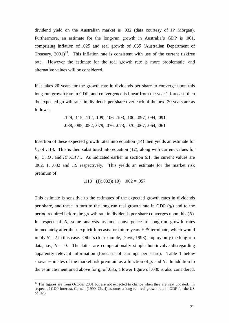
If it takes 20 years for the growth rate in dividends per share to converge upon this

long-run growth rate in GDP, and convergence is linear from the year 2 forecast, then

the expected growth rates in dividends per share over each of the next 20 years are as

follows:

.129, .115, .112, .109, .106, .103, .100, .097, .094, .091

.088, .085, .082, .079, .076, .073, .070, .067, .064, .061

Insertion of these expected growth rates into equation (14) then yields an estimate for

km of .113. This is then substituted into equation (12), along with current values for

Rf, U, Dm and ICm/DIVm. As indicated earlier in section 6.1, the current values are

.062, 1, .032 and .19 respectively. This yields an estimate for the market risk

premium of

057.062.)19)(.032)(.1(113. =−+

This estimate is sensitive to the estimates of the expected growth rates in dividends

per share, and these in turn to the long-run real growth rate in GDP (gr) and to the

period required before the growth rate in dividends per share converges upon this (N).

In respect of N, some analysts assume convergence to long-run growth rates

immediately after their explicit forecasts for future years EPS terminate, which would

imply N = 2 in this case. Others (for example, Davis, 1998) employ only the long-run

data, i.e., N = 0. The latter are computationally simple but involve disregarding

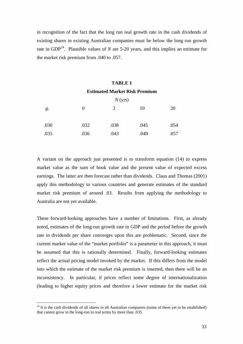
apparently relevant information (forecasts of earnings per share). Table 1 below

shows estimates of the market risk premium as a function of gr and N. In addition to

the estimate mentioned above for gr of .035, a lower figure of .030 is also considered,

23 The figures are from October 2001 but are not expected to change when they are next updated. Inrespect of GDP forecast, Cornell (1999, Ch. 4) assumes a long-run real growth rate in GDP for the USof .025.

33

in recognition of the fact that the long run real growth rate in the cash dividends of

existing shares in existing Australian companies must be below the long run growth

rate in GDP24. Plausible values of N are 5-20 years, and this implies an estimate for

the market risk premium from .040 to .057.

TABLE 1

Estimated Market Risk Premium

N (yrs)

gr 0 2 10 20

.030 .032 .038 .045 .054

.035 .036 .043 .049 .057

A variant on the approach just presented is to transform equation (14) to express

market value as the sum of book value and the present value of expected excess

earnings. The latter are then forecast rather than dividends. Claus and Thomas (2001)

apply this methodology to various countries and generate estimates of the standard

market risk premium of around .03. Results from applying the methodology to

Australia are not yet available.

These forward-looking approaches have a number of limitations. First, as already

noted, estimates of the long-run growth rate in GDP and the period before the growth

rate in dividends per share converges upon this are problematic. Second, since the

current market value of the “market portfolio” is a parameter in this approach, it must

be assumed that this is rationally determined. Finally, forward-looking estimates

reflect the actual pricing model invoked by the market. If this differs from the model

into which the estimate of the market risk premium is inserted, then there will be an

inconsistency. In particular, if prices reflect some degree of internationalization

(leading to higher equity prices and therefore a lower estimate for the market risk

24 It is the cash dividends of all shares in all Australian companies (some of them yet to be established)that cannot grow in the long-run in real terms by more than .035.

34

premium using this method), then this estimate will be too low for insertion into the

Officer version of the CAPM.

6.4 Summary

To summarise this review of evidence on the market risk premium in the Officer

CAPM, the estimates are .07 from historical averaging of the Ibbotson type, .056 from

historical averaging of the Siegel type, .07 from the Merton methodology, and .040-

.057 from the forward-looking approach. If a point estimate for the last approach is

.048, then the average across these four approaches is .061. In addition various other

methodologies have been alluded to, for which Australian results are not available but

which have generated low values in the markets to which they have been employed.

All of this suggests that the ACCC’s currently employed estimate of .06 is reasonable,

and no change is recommended.

7. Differential Taxation of Ordinary Income and Capital Gains

7.1 Modeling Differential Taxation

As previously discussed the Officer model assumes that ordinary income and capital

gains are equally taxed in Australia. The extent to which this assumption is false

depends upon the set of investors examined. The principal holders of Australian

equities are foreigners, companies, superannuation funds and individuals. As

discussed previously in section 4, on account of assuming that national capital

markets are segregated, recognition of foreign investors is both inconsistent and leads

to perverse results. Accordingly they are omitted from consideration. In respect of

corporate holdings of shares in other companies, inclusion of them would lead to

double-counting because the values of shares held by companies is already reflected

in the values of shares held by the other three classes of shareholders. Consequently

corporate owners of shares are ignored. Nevertheless, if companies were subject to

taxation on the dividends received from other companies, then the personal tax rates

faced by the ultimate recipients of dividends (individuals and superannuation funds)

would need to be increased to reflect this. However, companies are not taxed on

dividend income, and therefore this potential complication is absent. Thus, having

35

excluded both foreign investors and corporate shareholders, only individuals and

superannuation funds need to be considered.

In respect of individuals and superannuation funds there are three factors that suggest

that their taxes on capital gains will be considerably less than on ordinary income.

Firstly, it is probable that most of their equities are held for more than one year, and

therefore most of the resulting capital gains will be taxed at the concessionary “long-

term” rates. This is true despite an average turnover rate for Australian stocks in

recent years of around 50% (Australian Stock Exchange, 2001), because of wide

variation across investors in their holding periods25. To illustrate this point, suppose

10% of stock is traded four times a year and the rest is traded every ten years; the

turnover rate is then 50% but 90% of stocks are subject to long-term capital gains tax.

Secondly, in respect of these long-term gains, individuals are now subject to tax on

only 50% of the assessable gains, and superannuation funds on only 67% of them26.

Finally, capital gains are taxed only on realisation and the resulting opportunity to

defer payment of the tax is equivalent to a reduction in the statutory rate of tax.

Protopapadakis (1983) estimates that the opportunity to defer reduces the effective tax

rate on capital gains by about 50%.27 Collectively these features of investor behaviour

and the Australian taxation regime for capital gains suggest that, on average,

individual investors and superannuation funds will pay capital gains tax at only 25%

and 33% respectively of the rates applicable to ordinary income28.

These results suggest that a significant error in estimating the cost of capital may arise

from use of a model that assumes equal tax treatment of capital gains and ordinary

income. Furthermore the principle that capital gains are taxed less onerously than

ordinary income, because of exemptions and/or the deferral option, is well recognised,

25 Froot et. al (1992, Table 1) report variations across investor classes in the US ranging from one to sevenyears, the latter for passive pension funds. The variation across individual investors will be even morepronounced.26 Under the previous tax regime, only the real return was subject to tax.27 The result reflects the US tax regime in a period in which long-term capital gains (greater than one year)were subject to concessionary treatment similar to the current situation in Australia. Thus, prima facie, theresult is suggestive about the Australian situation. It should also be noted that the opportunity to deferlowers the effective tax rate not only because of the time value of money but also, as Hamson and Ziegler(1990, p. 49) note, because gains can be realised when the investor’s tax rate is lower, such as in retirement.

36

not only for Australia (see Howard and Brown, 1992) but other countries including

the US (see Constantinides, 1984) and the UK (see Ashton, 1991). Within New

Zealand this point is sufficiently acknowledged, and has been for several years, to the

extent that standard practice in estimating the cost of capital is to invoke a model

recognizing less onerous tax treatment of capital gains relative to ordinary income

(see, for example, New Zealand Treasury, 1997).

To determine whether recognition of this issue would materially alter the results from

the Officer model, it is necessary to construct a model of the cost of equity that allows

for differential tax treatment of capital gains and ordinary income. Various authors

have done so, including Ashton (1989, 1991), Lally (1992), Cliffe and Marsden

(1992), Dempsey (1996) and Brailsford and Davis (1995). However all of these

models treat dividend imputation as a process that lowers the tax rate on dividends

rather than the corporate tax rate. Consequently their cost of equity is defined over

returns exclusive of imputation credits. Consistency with the Officer model would

require that returns be defined to include imputation credits. Lally and van Zijl (2001)

have done this and the result is

em

mmfmfe T

DIVIC

UDTRkTDIVICUDTRk β

+−−−+

++−= 1)1(ˆ1)1(ˆ (15)

where D is the cash dividend yield for the company in question. In addition the

parameter T is a weighted average (across investors) of the following tax ratio

gi

gii

ttt

−−

1

where ti is the ordinary tax rate of investor i and tgi is their tax rate on capital gains

(this rate impounds the effect of the deferral option). Thus the parameter T is a

measure of the extent to which ordinary income is taxed more heavily than capital

gains29.

28 The 25% figure for individuals reflects all gains being taxed at the long-term rate, with a 50% exemptionand a further 50% reduction to reflect the deferral effect. The 33% figure for institutions is calculated in aparallel fashion.

37

Clearly the formula (15) is more complex than the Officer model (3), and the intuition

for the additional terms is as follows. The additional terms are of two types: firstly, a

dividend term for the firm in question, inclusive of imputation credits to the extent

they are usable (and its market counterpart inside the market risk premium term);

secondly, the riskfree rate Rf is replaced by Rf(1-T). In respect of the gross dividend

term, as this rises, the firm substitutes gross dividend for capital gain. The former is

taxed at the ordinary rate and the latter at the capital gains tax rate. If the ordinary tax

rate is higher than the rate on capital gains then the increase in gross dividend at the

expense of capital gain is disadvantageous in tax terms and therefore must be

compensated for by higher expected return. This is the effect of the dividend term. In

respect of the riskfree rate, to see the effect of this, assume that the dividend is zero.

Now consider the effect as beta goes to zero. Equation (15) says that the expected

return on equity goes to Rf(1-T), which is less than the riskfree rate. This occurs

because the firm’s equity resembles a riskless asset except that it is taxed as capital

gain rather than at the ordinary tax rate applicable to interest. If the tax rate on capital

gains is less than the ordinary tax rate (i.e., T is positive) then the expected return of

zero beta equity before personal tax does not need to be as high as Rf.

7.2 Comparison of Models

Whether equation (15) yields a materially different result to that of the Officer model

(3) depends on a number of factors. One of them is how the market risk premium is

estimated. One possibility is that the current value of km is estimated by the Siegel

(1992) or forward-looking methods, and then translated into an estimate of the market

risk premium using current values of the remaining parameters. In this event, models

(3) and (15) will involve the same estimate for km, and hence mk̂ . The excess of the

estimated cost of equity in (15) over that of the Officer model in (3), and denoted ∆,

will then be

+−+−

+=∆

m

mmfef D

ICUDRRDIVICUDT 11 β (16)

29 Equation (15) can also be obtained from Lally (1992, 2000b) by adding the imputation credits (to theextent they can be used) to his formula for the cost of equity.

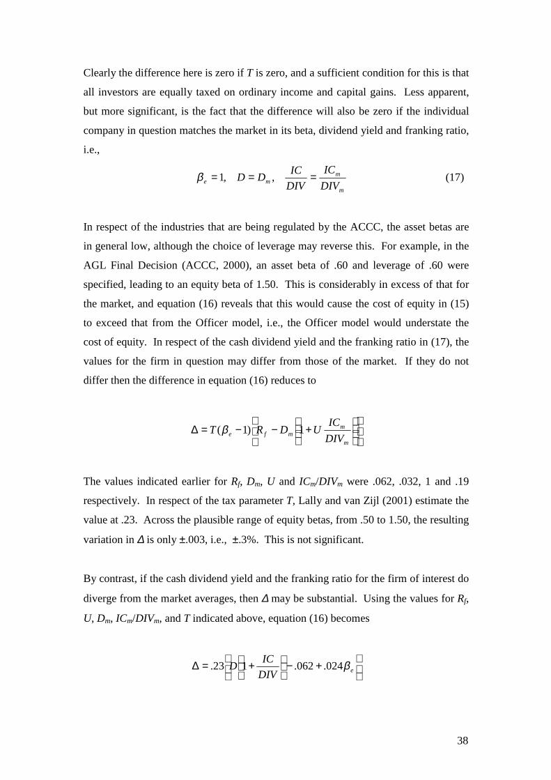
38

Clearly the difference here is zero if T is zero, and a sufficient condition for this is that

all investors are equally taxed on ordinary income and capital gains. Less apparent,

but more significant, is the fact that the difference will also be zero if the individual

company in question matches the market in its beta, dividend yield and franking ratio,

i.e.,

m

mme DIV

ICDIVICDD === ,,1β (17)

In respect of the industries that are being regulated by the ACCC, the asset betas are

in general low, although the choice of leverage may reverse this. For example, in the

AGL Final Decision (ACCC, 2000), an asset beta of .60 and leverage of .60 were

specified, leading to an equity beta of 1.50. This is considerably in excess of that for

the market, and equation (16) reveals that this would cause the cost of equity in (15)

to exceed that from the Officer model, i.e., the Officer model would understate the

cost of equity. In respect of the cash dividend yield and the franking ratio in (17), the

values for the firm in question may differ from those of the market. If they do not

differ then the difference in equation (16) reduces to

+−−=∆

m

mmfe DIV

ICUDRT 1)1(β

The values indicated earlier for Rf, Dm, U and ICm/DIVm were .062, .032, 1 and .19

respectively. In respect of the tax parameter T, Lally and van Zijl (2001) estimate the

value at .23. Across the plausible range of equity betas, from .50 to 1.50, the resulting

variation in ∆ is only ±.003, i.e., ±.3%. This is not significant.

By contrast, if the cash dividend yield and the franking ratio for the firm of interest do

diverge from the market averages, then ∆ may be substantial. Using the values for Rf,

U, Dm, ICm/DIVm, and T indicated above, equation (16) becomes

+−

+=∆ eDIV

ICD β024.062.123.

39

The bounds on a firm’s dividend yield D are zero to .08 (the latter is the outer limit of

observed yields on Australian companies when averaged over the last three years and

when averages that are significantly influenced by one year’s result are excluded).

The bounds on the franking rate IC/DIV are zero to .43 (the latter is the largest value

possible with a corporate tax rate of .30). Finally, plausible bounds on βe are .50 to

1.50. Using these bounds, the most extreme values for ∆ in the last equation are -.011

and .020.

We now consider the implications of estimating the market risk premium by historical

averaging of the Ibbotson type. In this case, one should determine the ex-post value

for the market risk premium for each year in a long time-series, and then average over

these. As we have indicated earlier, using data for the last 100 years, the result for the

Officer model is an estimate of about .07. For the model in (15) the estimate would

be

+−−− T

DIVICUDTRRAV

m

mmfm 1)1(ˆ

where AV[.] denotes the sample average over [.]. This is equal to

[ ] ( )[ ]

−−+− T

DIVICUDAVTDRAVRRAV

m

mmmffm

ˆ (18)

The first of these terms is the historical averaging estimate for the market risk

premium in the Officer model, i.e., .07. The last term is zero until 1987, because

imputation did not commence until then. This represents only 13 of the 100 years in

the data used for the historical averaging. Thus an estimate of it is 13% of the average

value since 1987. This will be close to zero, as follows. The market cash dividend

yield averaged .035 over this period (data courtesy of JP Morgan). Thus, even if the

franking ratio was as much as .50 and T was as much as .30, then with U = 1, the post

1987 average for the last term in (18) would only be .005. Multiplication by .13 then

yields less than .001, i.e., less than .1%. This can be ignored. The average in (18) is

then

40

( )[ ]TDRAV mf −+07. (19)

The last term in (19) is also close to zero because the estimate of T is well below one

and, over the last 100 years, the difference between the riskfree rate and the market

cash dividend yield has not been large. The average value for Rf over this period was

.064 (Dimson, 2000, Table 2). Also, the average for Dm was about .0430. If the

current estimate for T of .23 is attributed to the last 100 years, then the last term in

(19) becomes .005 and the average in (19) becomes .07531. The excess of the

estimated cost of equity in equation (15) over that of the Officer model in (3) is then

efRDIVICUDT β005.1 +

−

+=∆ (20)

If the dividend yield and the franking ratio for the firm of interest are similar to the

market averages (of .032 and .19) then, with U =1, T = .23 and the current value of Rf

of .062, the difference in (20) reduces to

eβ005.006. +−=∆

Across the plausible range of values for the equity beta, from .50 to 1.50, the value of

∆ departs from zero by only .004 at most. So, as with the situation in which the

market risk premium is estimated by the Siegel or forward-looking methods, the

difference between the estimated costs of equity from models (15) and (3) is slight.

However, if the firm’s values for D, IC/DIV or βe depart from the market averages,

then the excess in the estimated cost of equity from equation (15) over (3), as shown

in equation (20), could be substantial. To demonstrate this we use the values above

for Rf, U and T of .062, 1 and .23 respectively. In addition, we use the same bounds

30 Data on Dm over the entire period is not available but Datastream gives an average of .043 over theperiod since 1973.31 Clearly the Australian tax regime changes as one moves back through time over the last century. Inparticular, capital gains tax did not apply to individuals prior to 1986, and this would induce anincrease in T. However, it is also true that superannuation funds were not taxed on anything prior to1986, and this would induce a reduction in T. It is also true that, as one moves back in time, the ratesof tax on ordinary income tend to decline, and this also exerts a downward effect upon T. Takingaccount of all this, the current estimate for T of .23 seems reasonable as an upper bound estimate of theaverage value over the last 100 years.

41

used earlier for D, IC/DIV and βe of 0 to .08, 0 to .43 and .50 to 1.50. Accordingly the

difference in (20) could range from -.012 to .020.

7.3 Summary

In summary then, regardless of whether the market risk premium is estimated through

the Ibbotson, Siegel or forward-looking methods, the difference in the estimated cost

of equity from equations (3) and (15) is not significant if the cash dividend yield and

franking ratio for the firm of concern are similar to their market counterparts. If they

are not constrained to be similar, then the estimated cost of equity from (15) could

diverge from the Officer model by as much as -.011 to .020 if the market risk

premium is estimated through the Siegel or forward-looking methods, and by as much

as -.012 to .020 under the Ibbotson method. The results from these two estimation

approaches are pleasingly consistent. Clearly an increase in the cost of equity of .020

is significant. Nevertheless, even if it is true that the firm’s cash dividend yield and

franking ratio are unusual, there still remains the question of whether these parameter

values should be acknowledged. As indicated in section 5, when discussing the ratio

IC/TAX, it may not be desirable to use the firm’s actual values. The compromise

suggested there was to use the averages for the relevant industry. Applying the same

practice here involves using the relevant industry averages for D and IC/DIV, and this

will generate less extreme values for them. For example, if the maximum industry

average D (dividend yield) fell from .08 to .053, then the most extreme difference in

the costs from equity from models (3) and (15) would fall from .020 to .011.32

Whether effects up to this level justify a change in the model used is a matter for

debate. Clearly no consensus has yet developed amongst Australian academics and

practitioners for making such an adjustment, and it seems inappropriate for the ACCC

to lead in this area. Consequently the continued use of the Officer model is

recommended. Nevertheless, the suggestion that the cost of equity could be increased

by up to .011 may lead to some enthusiasm for the adjustment on the part of regulated

firms. However the argument for raising the utilization rate on imputation credits

from the present generally employed figure of .60 to 1 is at least as strong, and will

42

exert a countervailing effect upon the output price granted to a regulated firm. To

illustrate this, consider the simple example of a regulated firm in section 4. With a

utilization rate on imputation credits of .60 and a cost of equity of .12, the effective

tax rate Te and the valuation equation for the firm were as follows

[ ] 12.)60(.1130. =−=eT

03.12.

)12.1($.....)12.1(

)03.1)(12.1($12.1

)12.1($100$ 2 −−=+−+−= PmPmPmm

Solving the last equation yielded an output price of $10.23. If the cost of equity is

raised by .011, then the last equation becomes

03.131.)12.1($.....

)131.1()03.1)(12.1($

131.1)12.1($100$ 2 −

−=+−+−= PmPmPmm

and this implies that the output price rises from $10.23 to $11.48. However, if the

utilisation rate is raised to 1, then the effective tax rate falls to zero and the output

price drops back to $10.10, i.e., slightly less than the original $10.23.

In conclusion, no consensus has yet developed amongst Australian academics and

practitioners for making an adjustment for differential taxation of capital gains and

ordinary income, and it seems inappropriate for the ACCC to lead in this area.

Consequently the continued use of the Officer model is recommended. If such an

adjustment were made, it would raise the allowed output prices of some firms.

However the argument for raising the utilisation rate on imputation credits is at least

as strong, and the net effect of the two changes is unlikely to significantly benefit any

firm.

8. Conclusion

32 The largest industry average cash dividend yield in 2001 was .053 for “utilities” (data courtesy of JPMorgan).

43

This paper has examined a series of issues relating to the cost of equity under

dividend imputation. The conclusions are as follows. First, regarding the issue of

recognizing foreign investors, continued use of a version of the Capital Asset Pricing

Model that assumes that national equity markets are segmented rather than integrated

(such as the Officer model) is recommended. It follows that foreign investors must be

completely disregarded. Consistent with the disregarding of foreign investors, most

investors recognized by the model would then be able to fully utilize imputation

credits.

Second, regarding the appropriate adjustment to the company tax rate to reflect the

benefits of imputation, the utilization rate for imputation credits should be set at one,

and this follows from the first point above. In addition the ratio of imputation credits

assigned to company tax paid should be set at the relevant industry average, which

appears to be at or close to one for most industries. These two recommendations

imply an imputation adjusted company tax rate of zero rather than the generally

accepted figure of 50% of the statutory rate. Put another way, they imply that the

product of the utilization rate and the ratio of imputation credits assigned to company

tax paid (denoted gamma by the ACCC) should be at or close to 1 for most companies

rather than the currently employed figure of 0.50. The effect of this change would be

to reduce the allowed output prices of regulated firms.

Third, in respect of the market risk premium in the Officer model, the range of

methodologies examined give rise to a wide range of possible estimates for the market

risk premium and these estimates embrace the current value of 6%. Accordingly,

continued use of the 6% estimate is recommended.

Finally, regarding the differential taxation of capital gains and ordinary income, the

simplifying assumption in the “Officer” model that they are equally taxed at the

personal level could lead to an error in the estimated cost of equity of up to 1.1%,

depending upon the relevant industry average cash dividend yield and franking ratio.

Prima facie this is a sufficiently large sum to justify use of a cost of equity formula

that recognizes differential personal taxation of capital gains and ordinary income, and

such a formula is presented in this paper. However a consensus has not yet developed

amongst Australian academics and practitioners for making such an adjustment and it

44

seems inappropriate for the ACCC to lead in this area. Consequently the continued

use of the Officer model is recommended. If such an adjustment were made, it would

raise the allowed output prices of some firms. However the argument for raising the

utilisation rate on imputation credits is at least as strong, and the net effect of the two

changes is unlikely to significantly benefit any firm.

REFERENCES

Ashton, D. 1989, ‘Textbook Formulae and UK Taxation: Modigliani and MillerRevisited’, Accounting and Business Research, vol.19, pp.207-12.

_________ 1991, ‘Corporate Financial Policy: American Analytics and UKTaxation’, Journal of Business Finance and Accounting, vol.31, 465-482.

Australian Competition and Consumer Commission. 2000, Access Arrangement byAGL Pipelines (NSW) Pty Ltd for the Central West Pipeline.

___________________________________________ 2001, Final Decision: AccessArrangement Proposed by Epic Energy South Australia for the Moomba to AdelaidePipeline System.

Australian Department of Treasury. 1991, ‘Financial Monitoring of GovernmentBusiness Enterprises: An Economic Framework’, Treasury Economic Paper No. 14.

______________________________ 2001, Mid-Year Economic and Fiscal Outlook2000-01.

Australian Stock Exchange. 2001, ASX Fact Book.

Ball, R. and Bowers, J. 1988, ‘The Cost of Equity Capital under the AustralianImputation Tax System’, working paper.

Blume, M. 1974, ‘Unbiased Estimation of Long-Run Expected Rates of Return’,Journal of the American Statistical Association, vol.69, pp.634-38.

Bookstaber, R. and Pomerantz, S. 1991, ‘An Information-Based Model of MarketVolatility’, Financial Analysts Journal, Nov-Dec, pp.37-46.

Booth, L. 1999, ‘Estimating the Equity Risk Premium and Equity Costs: New Waysof Looking at Old Data’, Bank of America Journal of Applied Corporate Finance, Vol12 No. 1, pp. 100-112.

Brailsford, T. and Davis, K. 1995, ‘Valuation with Imputation’, JASSA, March, pp.14-18.

45

___________ Faff, R. and Oliver, B. 1997, Research Design Issues in the Estimationof Beta, McGraw-Hill Series in Advanced Finance, Volume 1, McGraw-HillAustralia, Sydney.

Brown, P. and Walter, T. 1986, ‘Ex-Dividend Day Behaviour of Australian SharePrices’, Australian Journal of Management, vol.11, pp.139-52.

________ and Clarke, A. 1993, ‘The Ex-Dividend Day Behaviour of AustralianShare Prices Before and After Dividend Imputation’, Australian Journal ofManagement, vol.18, pp.1-40.

Brown, S., Goetzmann, W. and Ross, S. 1995, ‘Survival’, Journal of Finance, vol.50,pp.853-73.

Bruckner, K., Dews, N. and White, D. 1994, ‘Capturing Value from DividendImputation’, McKinsey and Company.

Campbell, J. 1987, ‘Stock Returns and the Term Structure’, Journal of FinancialEconomics, vol.18, pp.373-99.

Chan, K., Karolyi, A. and Stulz, R. 1992, ‘Global Financial Markets and the RiskPremium on US Equity’, Journal of Financial Economics, vol.32, pp.137-67.

Cavaglia, S., Brightman, C. & Aked, M. 2000, ‘The Increasing Importance of IndustryFactors’, Financial Analysts Journal, Sept-Oct, pp. 41-54.

Claus, J. and Thomas, J. 1999, ‘The Equity Risk Premium is Much Lower than youthink it is: Estimates from a New Approach’, working paper.

____________________ 2001, ‘Equity Premia as Low as Three Percent?: Evidencefrom Analysts’ Earnings Forecasts for Domestic and International Stocks’, TheJournal of Finance, vol. 56, pp. 1629-1666.

Cliffe, C. and Marsden, A. 1992, ‘The Effect of Dividend Imputation on CompanyFinancing Decisions and the Cost of Capital in New Zealand’, Pacific AccountingReview, vol.4, pp.1-30.

Constantinides, G., 1984, Optimal Stock Trading with Personal Taxes: Implicationsfor Prices and the Abnormal January Returns, Journal of Financial Economics 13, 65-89.

Cooper, I. 1996, ‘Arithmetic Versus Geometric Mean Estimators: Setting DiscountRates for Capital Budgeting’, European Financial Management, vol.2, pp.157-67.

________ and Kaplanis, E. 1994, ‘Home Bias in Equity Portfolios, Inflation Hedgingand International Capital Market Equilibrium’, The Review of Financial Studies,vol.7, pp.45-60.

Copeland, T., Koller, T. and Murrin, J. 1994, Valuation: Measuring and Managingthe Value of Companies, J.Wiley & Sons Inc., New York.

46

Cornell, B. 1999, The Equity Risk Premium, John Wiley & Sons, New York.

Damodaran, A. 1997, Corporate Finance: Theory and Practice, John Wiley & Sons,New York.

Davis, K. 1998, The Weighted Average Cost of Capital for the Gas Industry, reportprepared for Australian Competition and Consumer Commission and Office of theRegulator General.

Dempsey, M. 1996, ‘The Cost of Equity Capital at the Corporate and Investor LevelsAllowing a Rational Expectations Model with Personal Taxation’, Journal of BusinessFinance and Accounting, vol.23, pp.1319-31.

Dimson, E., Marsh, P. and Staunton, M. 2000, ‘Twelve Centuries of Capital MarketReturns’, working paper.

Fama, E. and French, J. 1988a, ‘Permanent and Transitory Components of StockPrices’, Journal of Political Economy, pp.246-73.

_____________________ 1988b, ‘Dividend Yields and Expected Stock Returns’,Journal of Financial Economics, vol.22, pp.3-25.

______________________ 1989, ‘Business Conditions and Expected Returns onStocks and Bonds’, Journal of Financial Economics, vol.25, pp.23-49.

______________________ 2002, ‘The Equity Premium’, The Journal of Finance,vol. 57, pp. 637-659.

Frank, M. and Jagannathan, R. 1998, ‘Why do Stocks Prices Drop by less than theValue of the Dividend? Evidence from a Country Without Taxes’, Journal ofFinancial Economics, vol.47, pp.161-88.

French, K., Schwert, W. and Stambaugh, R. 1987, ‘Expected Stock Returns andVolatility’, Journal of Financial Economics, vol.19, pp.13-29.

Friend, I. and Blume, M. 1975, ‘The Demand for Risky Assets’, American EconomicReview, vol.65, pp.900-22.

Froot, K., Perold, A. and Stein, J. 1992, ‘Shareholder Trading Practices and CorporateInvestment Horizons’, Continental Bank Journal of Applied Corporate Finance, pp.42-58.

Glosten, L., Jagannathan, R. and Runkle, D. 1993, ‘On the Relation Between theExpected Value and the Volatility of the Nominal Excess Return on Stocks’, TheJournal of Finance, vol.40, pp.1779-1801.

Gordon, M. and Shapiro, E. 1956, ‘Capital Equipment Analysis: The Required Rate ofProfit’, Management Science, vol.3, pp.102-10.

47

_________ and Gould, L. 1984, ‘The Nominal Yield and Risk Premium on the TSE-300, 1956-1982’, Canadian Journal of Administrative Sciences, vol.1(1), pp.50-60.

Gray, S. 1999, Response to Consultation Paper No. 4: Cost of Capital Financing,submitted to the Office of the Regulator-General Victoria as part of the 2001Electricity Distribution Price Review.

Hamson, D. and P. Ziegler, 1990, The Impact of Dividend Imputation on Firms’Financial Decisions, Accounting and Finance 30, 29-53.

Harris, R. and Marston, F. 1992, ‘Estimating Shareholder Risk Premia UsingAnalysts’ Growth Forecasts’, Financial Management, vol.21 (2), pp.63-70.

________________________ 2001, ‘The Market Risk Premium: ExpectationalEstimates Using Analysts’ Forecasts’, working paper.

Hathaway, N. and Dodd, P. 1993, ‘Australian Public Sector Cost of Capital: A CriticalLook at the Treasury Model’, working paper, The University of Melbourne.

___________ and Officer, R. 1995, ‘The Value of Imputation Tax Credits’, workingpaper, University of Melbourne.

Harvey, C. 1991, ‘The World Price of Covariance Risk’, The Journal of Finance,vol.46, pp.111-57.

Howard, P. and R. Brown, 1992, Dividend Policy and Capital Structure under theImputation Tax System: Some Clarifying Comments, Accounting and Finance 32, 51-61.

Huberman, Gur. 2001, ‘Familiarity Breeds Investment’, The Review of FinancialStudies, vol. 14, pp. 659-680.

Ibbotson, R. and Sinquefield, R. 1976, ‘Stocks, Bonds, Bills and Inflation: Year-by-Year Historical Returns (1926-1974)’, Journal of Business, pp. 11-47.

Indro, D. and Lee, W. 1997, ‘Biases in Arithmetic and Geometric Averages asEstimates of Long-Run Expected Returns and Risk Premia’, Financial Management,vol. 26, no. 4, pp.81-90.

Jagannathan, R., McGrattan, E. and Scherbina, A. 2000, ‘The Declining US EquityPremium’, Federal Bank of Minneapolis Quarterly Review, vol. 24, pp. 3-19.

J. B. Were, 1996, Australian Equity Market Profile March 1996.

Jorion, P. and Goetzmann, W. 1999, ‘Global Stock Markets in the 20th Century’, TheJournal of Finance, vol. 54, pp. 953-980.

Kandel, S. and Stambaugh, R. 1987, ‘On Correlation and Inferences about Mean-Variance Efficiency’, Journal of Financial Economics, vol.18, pp.61-90.

48

Keim, D. and Stambaugh, R. 1986, ‘Predicting Returns in the Stock and BondMarkets’, Journal of Financial Economics, vol.17, pp.357-90.

Lally, M. 1992, ‘The CAPM Under Dividend Imputation’, Pacific AccountingReview, vol.4, pp. 31-44.

________ 1995, ‘The Accuracy of CAPM Proxies for Estimating a Firm’s Cost ofEquity’, Accounting and Finance, vol.35, pp. 63-72.

________ 1996, ‘The CAPM under Dividend Imputation and International PortfolioSelection’, Pacific Accounting Review, vol.8, pp. 48-65.

________ 1998, ‘The CAPM with Personal Taxes and International PortfolioSelection’, The New Zealand Investment Analyst, vol.19, pp. 22-24.

________ 2000a, ‘The Real Cost of Capital in New Zealand: Is it too High?’, NewZealand Business Roundtable, Wellington.

________ 2000b, The Cost of Equity Capital and its Estimation, McGraw-Hill Seriesin Advanced Finance, vol. 3, McGraw-Hill Australia, Sydney.

________ and van Zijl, A. 2001, ‘Capital Gains and the Capital Asset Pricing Model’,working paper, Victoria University of Wellington.

Lintner, J. 1965, ‘The Valuation of Risky Assets and the Selection of Investments inStock Portfolios and Capital Budgets’, Review of Economics and Statistics, vol.47,pp.13-37.

Lonergan, W. 2001, ‘The Disappearing Returns’, JASSA, Autumn, pp. 8-17.

McDonald, R. 2001, ‘Cross-Border Investing with Tax Arbitrage: The Case ofGerman Dividend Tax Credits’, The Review of Financial Studies, vol. 14, pp. 617-657.

Merton, R. 1980, ‘On Estimating the Expected Return on the Market’, Journal ofFinancial Economics, vol.8, pp.323-61.

Monkhouse, P. 1993, ‘The Cost of Equity under the Australian Dividend ImputationTax System’, Accounting and Finance, vol.33, pp.1-18.

____________ 1996, ‘The Valuation of Projects under the Dividend Imputation TaxSystem’, Accounting and Finance, vol. 36, pp. 185-212.

Mossin, J. 1966, ‘Equilibrium in a Capital Asset Market’, Econometrica, vol.24,pp.768-83.

New Zealand Treasury, 1997, Estimating the Cost of Capital for Crown Entities andState-Owned-Enterprises.

49

Odier, P. and Solnik, B. 1993, ‘Lessons for International Asset Allocation’, FinancialAnalysts Journal, March/April, pp. 63-77.

Officer, R. 1989. ‘Rates of Return to Shares, Bond Yields and Inflation Rates: AnHistorical Perspective’, in Share Markets and Portfolio Theory, 2nd edition, (Eds: RBall, F Finn, P. Brown and R. Officer), University of Queensland Press.

_________ 1994, ‘The Cost of Capital of a Company under an Imputation TaxSystem’, Accounting and Finance, vol.34, pp.1-17.

Pastor, L. and Stambaugh, R. 2001, ‘The Equity Premium and Structural Breaks’, TheJournal of Finance, vol. 56, pp. 1207-39.

Poterba, J. and Summers, L. 1988, ‘Mean Reversion in Stock Prices: Evidence andImplications’, Journal of Financial Economics, vol.22, pp.27-59.

Protopapadakis, A. 1983, ‘Some Indirect Evidence on Effective Capital Gains Taxes’,Journal of Business, vol.56, pp.127-38.

Ragunathan, V., Faff, R. and Brooks, R. 1999, ‘Australian Industry Beta Risk, theChoice of Market Index and Business Cycles’, Applied Financial Economics, vol. 10,pp. 49-58.

Roll, R. 1977, ‘A Critique of the Asset Pricing Theory’s Tests; Part I: On Past andPotential Testability of the Theory’, Journal of Financial Economics, vol. 4, pp. 129-76.

______ and Ross, S. 1994, ‘On the Cross-Sectional Relation Between ExpectedReturns and Betas’, Journal of Finance, vol.49, pp.101-21.

Schwert, G. 1990, ‘Stock Returns and Real Activity: A Century of Evidence’, Journalof Finance, vol.45, pp.1237-57.

Scruggs, J. 1998, ‘Resolving the Puzzling Intertemporal Relation Between the MarketRisk Premium and Conditional Market Variance: A Two-Factor Approach’, Journalof Finance, vol.53, pp.575-603.

Shanken, J. 1987, ‘Multivariate Proxies and Asset Pricing Relations: Living with theRoll Critique’, Journal of Financial Economics, vol.18, pp.91-110.

Sharpe, W. 1964, ‘Capital Asset Prices: A Theory of Market Equilibrium UnderConditions of Risk’, Journal of Finance, vol.19, pp.425-42.

Siegel, J. 1992, ‘The Equity Premium: Stock and Bond Returns since 1802’, FinancialAnalysts Journal, Jan-Feb, pp.28-38.

________ 1999, ‘The Shrinking Equity Premium’, Journal of Portfolio Management,Fall, pp. 10-17.

50

Solnik, B. 1974, ‘An Equilibrium Model of the International Capital Market’, Journalof Economic Theory, vol.8, pp.500-24.

Stambaugh, R. 1982, ‘On the Exclusion of Assets from Tests of the Two-ParameterModel: A Sensitivity Analysis’, Journal of Financial Economics, vol.10, pp.237-68.

Stulz, R. 1995, ‘The Cost of Capital in Internationally Integrated Markets: The Caseof Nestle’, European Financial Management, vol.1. pp.11-22.

Tesar, L. and Werner, I. 1995, ‘Home Bias and High Turnover’, Journal ofInternational Money and Finance, vol.14, pp.467-92.

Van Horne, J., Davis, K., Nicol, R. and Wright, K. 1990, Financial Management andPolicy in Australia, 3rd edition, Prentice-Hall, New York.

Walker, S. & Partington, G. 1999, ‘The Value of Dividends: Evidence from Cum-Dividend Trading in the Ex-Dividend Period’, Accounting and Finance, vol. 39, pp.275-96.

Welch, I. 2001, ‘The Equity Premium Consensus Forecast Revisited’, working paper.

Wood, J. 1997, ‘A Simple Model for Pricing Imputation Tax Credits under Australia’sDividend Imputation Tax System’, Pacific-Basin Finance Journal, vol.5, pp.465-80.