The Cost of Banking Regulation∗

Luigi Guiso

European University Institute, Ente Einaudi, and CEPR

Paola Sapienza

Northwestern University, NBER, and CEPR

Luigi Zingales

University of Chicago, NBER, and CEPR

February 2007

Abstract

We use exogenous variation in the degree of restrictions to bank competition across Italian provinces to

study both the effects of bank regulation and the impact of deregulation. We find that where entry was

more restricted the cost of credit was higher and - contrary to expectations - access to credit lower. The

only benefit of these restrictions was a lower proportion of bad loans. Liberalization brings a reduction in

rate spreads and an increased access to credit at the cost of an increase in bad loans. In provinces where

restrictions to bank competition were most severe, the proportion of bad loans after deregulation raises above

the level present in more competitive markets, suggesting that the pre-existing conditions severely impact

the effect of liberalizations.

∗We are grateful to the Foundation Banque de France for funding this paper and we thank the seminar participants at theUniversite de Paris 1 Pantheon Sorbonne where the final project was presented. We thank Patricia Ledesma, Marco Pagano, andFabio Schiantarelli and participants at the Bank of Italy conference “Financial Structure, Product Market Structure and EconomicPerformance” and the Lisbon European Banking History conference. Luigi Guiso thanks the EEC and MURST for financialsupport, while Luigi Zingales thanks the Center for Security Prices and the Stigler Center at the University of Chicago for financialsupport.

1

As Barth, Caprio and Levine (2006) exhaustively document, the banking sector is probably the most

intensely regulated sector throughout the world. This is hardly surprising. If we espouse a benign view of

government regulation, there are several rationales that justify a government intervention. But the same is true

if we think government intervention is driven by political and electoral interests, rather than by the desire to

address market inefficiencies. The two views of government interventions obviously differ in their implications:

one predicts a positive effect of government regulation, the second a negative one.

In spite of the opposite predictions, these two views of regulation are hard to disentangle empirically.

According to the benign view of regulation, governments intervene more where markets fail more. Hence,

any attempt to estimate the effects of bank regulation would spuriously attribute a negative effect to bank

regulation unless the pre-existing degree of market failure is controlled for (an almost impossible task). Only

if the extent of regulation was exogenously imposed, we could hope to identify the true effect of regulation.

In this paper we claim that the Italian banking law of 1936 represents such a natural experiment. Introduced

after major bank failures, the 1936 law had the objective of enhancing bank stability through severe restrictions

on competition. While homogeneously imposed throughout the country, these restrictions had different impact

in different areas, because they granted a different flexibility to expand to different types of banks. Thus, an

unintended consequence of the law was a different degree of competition across Italian provinces, determined on

the basis of the conditions pre-existing the 1936 law. We exploit this exogenous variation to assess the impact

that restrictions on competition have on the structure of the banking industry. Since all these regulations

were removed during the 1980s, we also exploit this difference in the starting points to assess how differentially

repressed financial systems respond to liberalization.

We first establish that the 1936 banking law curtailed competition in Italian banking industry pre deregu-

lation (i.e., pre 1990s) and differentially so depending on the type of banking institutions present in 1936. In

particular, the interest rate spread (lending minus deposit rate) charged to customers in different provinces (a

measure of monopoly power) is directly related to measures of banking structure in 1936.

Then, we use a local indicator of the interest rate spread pre-deregulation as a measure of lack of competition

and we study the effect of this lack of competition on the functioning of the banking industry and the real

economy. We find that in provinces where there was more competition there was more access to credit (contrary

to what predicted by Petersen and Rajan, 1995) for both households and firms, more firms, and higher growth.

Consistent with the goals of the 1936 Banking Law, we find that provinces where there was less competition

1

experience a lower percentage of bad loans. Finally, consistent with Jayaratne and Strahan (1996), we find

that competition does not impact the quantity of loans.

Between the late 1980s and early 1990s Italy experienced several banking reforms. Entry was liberalized

(1990), the separation between short and long-term lending was removed (1993), the savings and loans legal

structure was transformed into a normal corporation, facilitating acquisition and mergers (1993), and starting

in 1994, all the major state-owned banks were privatized. Hence, we study the effect of deregulation as a

function of the level of competition in the banking sector before deregulation. We find that provinces that had

a less competitive banking sector during the regulation period experience a significant increase in the number

of households with access to credit. They also experience a reduction in the cost of borrowing, and an increase

in the percentage of bad loans. The overall effect is that after deregulation the provinces that were more

penalized by the restrictions in competition experience a higher-than-normal aggregate growth rate.

We are not the first to identify the costs of bank regulation. The closest papers to ours are Jayaratne and

Strahan (1996), Dehejia and Lleras-Muney (2005), and Guiso et al. (2004). The first two papers use the cross

sectional variation in banking regulation across U.S. states to assess the impact of financial development on

growth. The major difference is that U.S. states are free to choose their own regulation. Hence, it is difficult to

disentangle the effect of regulation from the effects of the political and economic conditions that lead regulation

to be enacted or lifted. Such problem does not exist in our sample, since the legislation is homogenous and

we use the cross sectional difference in the tightness of this regulation. As we discuss in the text, this cross

sectional difference in tightness is determined by historical accidents and is unlikely to be correlated with the

phenomena we study. As Guiso et al. (2004), we use the cross sectional variation in regulation across Italian

provinces as an instrument. That paper, however, only focuses on the effect of access to credit on aggregate

growth during the regulation period. By contrast, in this paper we measure the degree of competition across

different local markets and relate it to several characteristics of the banking industry, as well as aggregate

growth, both before and after deregulation. In so doing we are better able to study the cost and benefits of

banking regulation.

Our paper can also be seen as a within country analog of Demirguc-Kunt, Laeven, and Levine (2004),

who study the effect of banking regulation on the cost of credit across countries. They find that regulation

increases the cost of credit but this effect disappears once they control for property rights protection, leading

them to conjecture that banking regulation may reflect broader features of a country approach to competition.

2

Our within country approach enables us to disentangle these two effects and isolate the costs (as well as the

benefits) of banking regulation.

Our paper is also related to Bertrand, Schoar and Thesmar (2007) who analyze the effects of banking

deregulation on the industrial structure in France in the 1980s. Their advantange is that they can rely on

firm-level data to trace the effect of financial liberalization on entry and exit. Our paper focuses instead on the

effect of banking regulation and deregulation on the structure of the banking industry. The advantage of our

research design is the exogeneity of the tightness of regulation, which gives us an opportunity to shed some

empirical light on the trade off between banking competition and banking stability studied by Allen and Gale

(2004).

The rest of the paper proceeds as follows. Section 1 provides a brief history of Italian banking regulation.

Section 2 describes the data. Section 3 shows that the 1936 Banking Law had an enduring effect on bank

competition, which translated into higher markups. Section 4 analyzes the impact that the different levels of

competition had on access to credit, quantity of credit, percentage of bad loans, and aggregate growth. Section

5 repeats a similar analysis focusing on how the initial conditions affected the impact of deregulation. Section

6 concludes.

I The History of Italian Banking Regulation

In response to the 1930-31 banking crisis, in 1936 Italy introduced a new banking law, which imposed rigid

limits on the ability of different types of credit institutions to open new branches and extend credit. According

to the law, each credit institution was assigned a geographical area of competence based on its presence in

1936 and its ability to grow and lend was restricted to this area. A further directive, issued in 1938, regulated

differentially the ability of these institutions to grow. National banks could open branches only in the main

cities; cooperative and local commercial banks could only open branches within the boundaries of the province

they operated in 1936, while savings banks could expand within the boundaries of the region - which comprises

several provinces - they operated in 1936. Furthermore, each of these banks was required to try and shut down

branches located outside of its geographical boundaries.

As Table 1 shows, this regulation deeply affected banks’ ability to grow. Between 1936 and 1985 the

total number of bank offices grew 87%. During the same period, the number of bank offices in the United

3

States increased by 1228%.1 But Table 1 also shows that different types of banks grew at a different rate.

Savings banks and cooperatives’ (both local banks) offices grew on average 138%, while big national banks

grew only 70%. Since these types of banks differ only in their legal structure but not in their functions, it is

hard to explain these differential growth rates with different growth in the demand for their service. A more

plausible explanation is that regulation allowed savings banks more latitude to grow. This regulation remained

substantially unchanged until the end of the 1980s.

We will exploit these differences in the tightness of financial regulation across local credit markets to study

the effects of restriction on competition. For this variation to be a good natural experiment, however, we

need to show that i) the number and composition of banks in 1936 is not linked to some characteristics of

the region that affect the ability to do banking in that region and of firms to grow; ii) this regulation was not

designed with the needs of different regions in mind, but it was “random”; iii) the reason why this regulation

was maintained until the end of the 1980s has nothing to do with the actual needs of different regions.

A Why Regions Differ in their Banking Structure in 1936

As discussed in Guiso et al. (2004), the number of bank branches in 1936 was not an equilibrium market

outcome, but the result of a Government-directed consolidation during the 1930-33 crisis. The Italian Govern-

ment bailed out the major national banks and the savings banks, but chose to let smaller commercial banks

and cooperative ones fail.

Furthermore, the regional diffusion of different types of banks reflects the interaction between the subse-

quent waves of bank creation and the history of Italian unification. The high concentration of savings banks

in the North East and the Center, for instance, reflects the fact that this institution originated in Austria and

expanded first in the territory dominated by the Austrian Empire (Lombardia and the North East) and in the

nearby states, especially Tuscany and the Papal States. By contrast, two of the major national banks (Banca

Commerciale and Credito Italiano) were the result of direct German investments in the most economically

advanced regions at the time (Lombardia and Liguria).

As a result, as Guiso et al. (2004) show in Table 4, the four indicators of banking structure in 1936 - the

number of total branches (per million inhabitants) present in a region in 1936, the fraction of branches owned

by local versus national banks, the number of savings banks, and the number of cooperative banks per million

1See the Federal Deposit Insurance Corporation’s Historical Statistics on Banking, http://www2.fdic.gov/hsob

4

inhabitants – are not correlated with economic development in 1936, once we control for a South dummy that

is equal to one for regions south of Rome.

B Why Did the 1936 Law Favor Savings Banks?

There are two reasons why the Fascist regime favored savings banks. First, savings banks were non-profit

organizations, which had to distribute a substantial fraction of their net income to “charitable activities”.

Until 1931 these donations were spread among a large number of beneficiaries. Subsequently, however, the

donations became more concentrated toward political organizations created by the Fascists, such as the Youth

Fascist Organization and the Women Fascist Organization (Polsi, 2000). Not surprisingly, the Fascist regime

found convenient to protect its financial supporters!

The second reason is that the 1930-33 banking crisis was mainly due to the insolvency of major national

banks. This fear of the disastrous consequences of the failure of large banks created in the legislator a natural

bias against large banks.

C Why Was This Structure Maintained For So Long?

These differential restrictions, thus, have a clear rationale within the Fascist regime. But when in 1946 the

Bank of Italy restarted to authorize the creation of new branches, “the new authorizations were mainly given

to savings banks and – to a smaller extent – to cooperative banks and local commercial banks” (Cotula and

Martinez Oliva, 2003). Hence, the two biases exhibited by the Central Bank during the Fascist period –hostility

toward national banks and favor towards Savings Banks – continued after the war. Why? All the historians

mention the quest for stability as an important factor. The memories of the 1930s crisis were still very vivid in

the Central Bank administration and continued to inform its action. This explanation could at best account

for the hostility towards large national banks, but what about savings banks? One opinion – prevalent among

historians inside the Central Bank – is that this policy was aimed at promoting the investment of local savings

in loco, supporting the less developed areas (Albareto and Trapanese, 1999). This argument, however, is based

on the wrong assumption that excess deposits cannot be “recycled” in the interbank market, as it indeed

occurred. A second, more credible, interpretation has it that Donato Menichella (governor of the Bank of Italy

from 1948 to 1960) promoted the development of local banks at the expenses of national State-owned banks

“for the desire to see the power of the Central Bank vis-a-vis the banking system strengthened” (De Cecco,

5

1968, p. 67). De Cecco, however, is not entirely clear on the channel through which this relation worked.

One possibility is that stronger national banks could acquire too much lobbying power vis-a-vis the Governor,

reducing his autonomy. Another possible channel is the institutional structure of the Bank of Italy. After 1936

the Bank of Italy was formally owned by the State-owned national banks and by the Savings banks, which

jointly elected the Central Bank’s Board. The Board nominated the Governor, who was subject to the approval

of the Government. Since the State-owned national banks were much more concentrated, by increasing the

power of the fragmented Savings banks, the Governor could play a ”divide et impera” strategy, to maximize his

autonomy. Regardless of the specific channel, however, this interpretation suggests that the hostility against

the big national bank was not determined by economic reasons, but was the result of a power struggle within

the Government bureaucracy. While both the previous arguments have some merits, we think that the main

reason for these policy biases is that the Christian Democratic party inherited the political clientele of the

Fascist Party, including the network of local notables and the right to direct Savings Banks’ donations to the

favorite charitable organizations. By inheriting this network, the Christian Democratic party inherited also

the Fascists’ party interest in promoting Savings Banks at the expenses of all the other types of banks. The

Savings Banks also maintained their advantageous position relatively to other local banks because they were

government owned. After the Second World War government banks were controlled by politics and especially

from the mid-fifties the practice of political appointments of top executives in state-owned banks became the

way for politics to insure strong ties with the public banking system (Sapienza, 2004).

D The Deregulation Process

This regulatory system was maintained almost unchanged until the late 1980s. What triggered change was

the process of European integration and in particular the prospect of the application of the European Banking

Directive, mandating free entry, scheduled to be introduced in 1992. In anticipation of this change, the

procedure to open new bank offices was eased in 1986. Instead of requiring an explicit authorization of the

Bank of Italy, the authorization was considered granted unless explicitly denied within 60 days from the

request.

Entry was then entirely liberalized in 1990. In 1993 a new banking law (incorporating the Banking European

Directive) was approved. The separation between short and long-term lending was removed and banks were

allowed to underwrite security offerings and own equity. The same year, the legal structure of savings banks was

6

changed. From mutual organizations, they were transformed into standard corporations, facilitating acquisition

and mergers. Finally, in 1994 the Government started to privatize all the major State-owned banks.

II Data Description

To capture different aspects of the problem in this paper we use four main different data sources.

To measure the number of registered firms, their rate of formation, and the incidence of bankruptcy by

province we collected data coming from the Italian Statistical Institute (ISTAT) from a yearly edition of ”Il

Sole 24 Ore”, a financial newspaper. Table 2a reports summary statistics for these data. The Italian territory

is divided into 20 regions and each region is made up of a several provinces. New provinces have been created

over time up to 103 provinces; however, since our data go back in time we will be working with the 95 province

classification reconstructing the more recent data in order to be compatible with the old classification of

provinces.

The second dataset, is the Survey of Households Income and Wealth (SHIW). This survey, conducted

every two years by the Bank of Italy on a representative sample of about 8,000 households, collects detailed

information on Italian household income, consumption, and wealth and portfolio allocation across financial

instruments. For each household, the data also contain information on characteristics of the households’ head,

such as education, age, place of birth, and residence. An interesting feature of this survey is that each household

is asked to report whether it faced any problem in obtaining loans from financial intermediaries. We use this

information to create an indicator variable for households that were rationed in the market either because were

turned down or discouraged from borrowing. Table 2b reports the summary statistics for this sample.

The third dataset draws data from the 1988-2001 Survey of Investment in Manufacturing Firms (SIM)

which is run yearly by the Bank of Italy on a sample of about 1,000 firms with at least 50 employees. The

main purpose of the survey is to collect information on firms fixed investment, realized and planned for the

future. It also collects information on firms’ demographics and hiring and firing decisions. Since 1988, the

Survey of Investment in manufacturing asks questions on access to the loans market similar to those asked to

households in the SHIW, allowing us to construct an indicator for whether the firm was rationed in the loans

market. Table 2c shows summary statistics for this dataset.

Finally, the fourth dataset contains financial information about firms. It is from Centrale dei Bilanci

7

(CB), which provides standardized data on the balance sheets and income statements of about 30,000 Italian

non-financial firms. Data, available since 1982, are collected by a consortium of banks interested in pooling

information about their clients. A firm is included in the sample if it borrows from at least one of the banks

in the consortium. The database is highly representative of the Italian non-financial sector: a report by

Centrale dei Bilanci (1992), based on a sample of 12,528 companies drawn from the database (including only

the companies continuously present in 1982-90 and with sales in excess of 1 billion Lire in 1990), states that

this sample covers 57 percent of the sales reported in national accounting data. In particular, this dataset

contains a lot of small (less than 50 employees) and medium (between 50 and 250) firms

For some of the years prior to liberalization we have been able to merge the CB data data from the Credit

Register and thus obtain information on the interest rate charged by each bank (among those reporting to the

credit register which account for about 80% of total loans) that lends to the firms in our sample. In addition,

we can identify a number of characteristics of the lending banks, such as their size, profitability and relevance

of non-performing loans, by linking the merged dataset to an additional database that contains information

on the banks balance sheets. Table 2d reports the summary statistics for these data.

III The Effects of Banking Regulation on Competition

We want first to establish that regulation of bank entry designed in 1936 affected the working of the banking

industry before deregulation, i.e. until the late 1980s. To this purpose, we start by testing whether the

characteristics of the 1936 banking system have any impact on the structure of the banking industry along

two dimensions: the number of bank offices and the level of interest rates.

To characterize the regional structure of the banking system in 1936 and thus the tightness of regulation we

use four indicators that are inspired by the 1936 Inter-ministerial Committee for Credit and Savings (CICR)

anti-competitive regulation: (1) the number of bank branches per 1000 inhabitants in the region in 1936 (regions

with more branches in 1936 should have suffered less from the freeze); (2) the share of bank branches owned by

local banks over total branches in a region as of 1936 (the higher this ratio the less binding the CICR regulation

should have been); (3) the number of savings banks (the higher the number of Savings banks in 1936, the less

tight the 1936 regulation was); and (4) the number of cooperative banks per thousand inhabitants in the region

in 1936 (conditional on the proportion of local banks, cooperative banks were relatively disadvantaged in their

8

ability to grow). If the 1936 law had any bite, we should find opposite effects of these last two indicators.

A Effects on the number of bank offices

To assess the effects of differences in the bite of regulation on the level of the banking activity, Table 3 regresses

the number of bank offices in a province in 1985, before deregulation started, on the 1936 local bank structure.

As Table 3 column I shows, provinces with more bank branches per thousand inhabitants in 1936 also have

more bank branches per thousand inhabitants in 1985. This is hardly surprising, since it might simply reflect

that certain provinces are richer and so have more banks. But this effect persists, albeit smaller, even after we

control for the logarithm of the value added per capita in the province (column II). Even this reduced effect

is very noticeable quantitatively. A province that started with a level of bank branches per inhabitant one

standard deviation higher in 1936 had 17% more bank offices per inhabitants in 1985.

More interestingly, the proportion of bank offices controlled by local banks in 1936 affects the number of

bank offices present in 1985. As we said, local banks were given more room to expand locally compared to

national banks. This could explain why the total number of bank offices increased more in provinces where in

1936 the banking market was dominated by local banks. This effect is also quantitatively large. One standard

deviation increase in the fraction of branches controlled by local banks in 1936 leads to a 6 percentage points

increase in the number of bank branches per inhabitants in 1985 (a 20% increase).

As we said, among local banks the 1936 law granted more room to expand to savings banks, rather than

to cooperative banks. Once we control for the fraction of branches controlled by local banks this distinction

does not seem to make a big difference. As expected, in column I the coefficient on the number of cooperative

banks is negative and statistically significant, but when we insert the log of the GDP per capita the significance

disappears.

These four variables that summarize the structure of the banking system in 1936 can explain 27 percent

of the provincial variation in the number of bank branches before liberalization. Importantly, this effect is

not just a North-South divide. While ceteris paribus Southern provinces have fewer bank offices (see column

III of Table 3), the level of bank offices per inhabitant and the proportion of local banks remain statistically

significant after we insert a South dummy.

9

B Effect on the Cost of Credit

The second aspect we investigate is the effect of the 1936 law on the cost of credit. Table 4 presents some

estimates using the matched firms-bank register data that allow us to obtain a measure of the interest rate

on credit lines charged by each of the banks lending to a given firm. Since we do not have data for the

year 1985 we use data for the 1991, the earliest available year, before many of the liberalization steps were

undertaken. This assumption is supported by Angelini and Cetorelli (2003), who, by using bank-level balance

sheets, convincingly show that mark ups in the Italian banking industry remained unchanged until 1992, and

declined only after the liberalization started to unfold.

The dependent variable is the interest rate charged by each bank to each client. To control for differences

in riskiness across firms we insert a firm’s return on sales, its leverage, and its size (measured as log sales) as

explanatory variables. In addition, we also control for the Altman Z-score, which captures the probability of

bankruptcy, where a larger score value reflects a higher probability of default. This score is computed by CB

and is used by the banks belonging to the CB consortium to price their loans. Finally, we control for three

bank characteristics – size, share of non-performing loans and return on assets – which capture differences in

bank’s market power and efficiency that may be reflected in interest rates on loans.

The first two columns show that the loan rates paid by firms are affected by the bottlenecks created by

the 1936 law. The strongest effect is due to savings banks. In provinces where savings banks were more in

1936, we observe a lower spread between loans and deposits in 1991. By contrast firms in provinces where

cooperative banks were more diffuse in 1936, face, ceteris paribus, higher lending rates in the 1980s.

These effects are also economically significant. One standard deviation increase in the number of savings

bank per million inhabitants in 1936 reduces the lending rate by 239 basis points, while one standard deviation

increase in the number of cooperative banks in increases the lending rate by 157 basis points. Demirguc-

Kunt, Laeven, and Levine (2004) also find that banking regulation increases the cost of credit using cross

country variation. However, they also find that this effect disappears once they control for national indicators

of property rights protection, leading them to argue that banking regulation reflects broader features of a

country approach to competition. Our approach, based on within country variation in the bite of regulation,

is able to separate the effect of banking regulation on the cost of credit from other institutional features which

are automatically controlled for.

One potential problem is that the bank controls are few and the characteristics of 1936 banking structure

10

may be capturing unobserved bank characteristics that are relevant for interest rate setting, such as efficiency.

Since the same bank lends to multiple firms in different provinces we can account for unobservable bank

characteristics by adding bank fixed effect. When we do this in columns III and IV results are similar to those

in the first two columns.

In sum, the restrictions on entry imposed by the 1936 legislation seem to have substantially affected the

degree of local competition in the banking industry until the end of the 1980s. Having established this, we

can now study the effect of this lack of competition on the allocation of credit and, ultimately, on economic

growth. To do so, however, we need to construct a meaningful measure of the degree competition of the local

credit markets before deregulation and show that this measure of competition differs depending on how strong

was the effect of the 1936 regulation on the various local markets. Only after doing so can we analyze the real

impact of competition, using the structure of local credit markets in 1936 as instruments.

C Measuring competition in local credit markets

As a measure of competition we use a bank’s ability to charge its clients above its marginal cost (i.e., its

spread or mark up over the deposit rate).2 We use the CB data merged with the credit register to compute

the mark-up on deposit rates that a bank can charge to a given firm. This is computed by subtracting the

average rate on deposits in a province from the interest rate on the loans paid by the firm. Differences in this

spread could be due to differences in banks’ market power or differences in the riskiness of local borrowers.

In order to isolate the first effect from the second, we run regressions where we control for a number of

indicators that capture firms quality: the firm return on sales, its leverage (as a proxy for financial fragility),

its size (measured by log assets), which captures the fact that smaller firms are more likely to fail, and the

firm propensity score. For our purposes of controlling for the firm risk, the latter is a particularly important

variable. It is directly computed by the CB in order to obtain a synthetic indicator of the probability of default.

This score is then used by the banks that belong to the CB consortium to decide whether to grant a loan and

to price it. It is likely, thus, to capture most of the information on which banks condition for assessing firms’

risk.

Besides controlling for these firm characteristics we also include several bank controls: the size of the

lending banks (measured by log assets), its returns on assets, the ratio of non-performing loans on total loans

2The reason why most studies use a Herfindhal index of loans or deposits is that they do not have access to the bank-firm datawe have access to. Our measure speaks more directly to the effective market power banks have at a local level.

11

outstanding, and dummies for state or local government bank ownership (the first dummy is equal to 1 if the

bank is a savings bank, the second is equal to 1 if the bank is state-owned). These variables may affect the loan

rate as they capture differences across banks that are not picked up by the average deposit rate in a province.

For example, state-ownership of banks affects the lending rate, as state owned bank subsidize loans3; similarly,

bank profitability and non-performing loans affect the bank’s cost of raising funds.

To measure differences in the competition across local markets we insert a full set of dummies, one for

each Italian province for a total of 96 dummies, and take the coefficient on the province dummy as a measure

of the market power enjoyed by the banks lending in that market. The presumption is that the province – a

geographical unit close in size to a US county – is the relevant local market. There are two reasons why this

assumption is reasonable. First, according to the Italian antitrust authority the “relevant market” in banking

for antitrust purposes is the province. Second, this is also the definition the Central Bank used until 1990 to

decide whether to authorize the opening of new branches.

To transform the measure of market power into an indicator of the degree of competition in the local

credit markets we compute Competition = max(coefficient on provincial dummies) – (coefficient on provincial

dummies) so that the least competitive local market is standardized to zero and the units of the measure

of competition are deviations of the interest rate spread from the province where it is largest. Obviously, if

provincial markets were not geographically segmented – e.g. because firms could indifferently borrow in any

local market and could thus arbitrage away differences in lending rates – the coefficients on the provincial

dummies should not differ from each other. Thus, finding that these coefficients are indeed different can be

regarded as a test of local market segmentation. The F statistics for the hypothesis that the province effects

are equal to zero is 7,556.35 ( p-value = 0.0000), suggesting significant geographical dispersion in banking

competition.

Table 5, Panel A, lists our measure of local market competition sorting provinces from the least to the most

competitive one. The range of variation implies that in the most competitive province (Ravenna) the interest

rate spread is, ceteris paribus, 363 basis points lower than in the least competitive province (Catanzaro) while

in the median province the spread is 192 basis points lower than in the least competitive. The magnitude of

these figures implies that prior to liberalization local credit markets were markedly segmented.

Figure 1 shows visually how banking competition differs across local credit markets. While a North-South

3See Sapienza (2004).

12

divide is a clear feature of the data, there is considerable variation in the degree of competition suggesting

that one can rely on variation within the Center-North and the South to identify the effect of competition on

banking outcomes.

Table 5, panel B, shows how differences in the tightness of the 1936 regulation across regions has affected

banking competition. The first column regresses our measure of competition on the four indicators of 1936

regulation. In areas with more local banks and more savings banks and thus with less restricted opportunities

to compete in local markets, interest rate spreads are lower. A one standard deviation increase in the number

of bank offices belonging to local banks in 1936 lowers the spread by 18 basis points while a one standard

deviation increase in the number of savings banks per capita lowers the spread by 22 basis points. The number

of cooperative banks has, as expected, a negative impact on the degree of competition in the local credit

market but is not statistically significant. Similarly, the number of bank offices in 1936 has a positive effect

but not statistically significant. Overall, these 1936 variables explain 27 percent of the variation in the degree

of competition 50 years later. The hypothesis that they are jointly significantly equal to zero can be rejected

at conventional levels of significance, as shown by the value of the F -test.

The second column shows results when the two insignificant variables in the first regression are dropped; the

amount of variation explained falls to 22 percent but remains substantial even if only these two characteristics

of the 1936 banking structure are used to predict competition. The F -statistic for the joint significance of

these two variables raises to 14.24.

In the third column, we regress our competition index on the indicator of local credit market development

constructed by Guiso, Sapienza and Zingales (2004), based on the ease of access to credit. These two measures

are highly, but imperfectly, correlated suggesting that cost and availability of credit are two separate aspects

of a credit market.

IV The Effects of Restrictions on Bank Competition

In the previous section we have shown how the peculiarities of the Italian Banking Law of 1936 affected the

degree of bank competition at the provincial level. This link allows us to treat the component of the variation

in bank competition explained by the 1936 law as a random treatment. Hence, we can study how arbitrary

variations in the degree of competition across otherwise identical provinces can affect the allocation of credit

and, ultimately, economic performance. To this purpose, we will look at the effect of competition on a number

13

of indicators of banking and economic performance. Interestingly, we can do this exercise both for the regulated

period and for the deregulation period. We start with the regulated period.

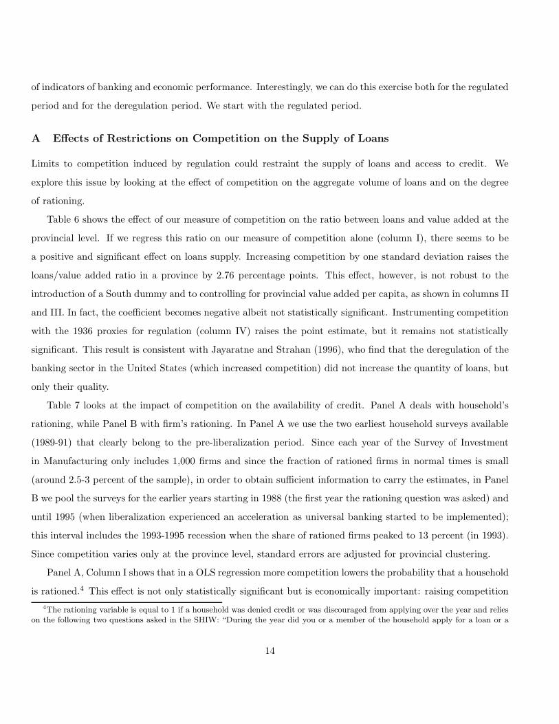
A Effects of Restrictions on Competition on the Supply of Loans

Limits to competition induced by regulation could restraint the supply of loans and access to credit. We

explore this issue by looking at the effect of competition on the aggregate volume of loans and on the degree

of rationing.

Table 6 shows the effect of our measure of competition on the ratio between loans and value added at the

provincial level. If we regress this ratio on our measure of competition alone (column I), there seems to be

a positive and significant effect on loans supply. Increasing competition by one standard deviation raises the

loans/value added ratio in a province by 2.76 percentage points. This effect, however, is not robust to the

introduction of a South dummy and to controlling for provincial value added per capita, as shown in columns II

and III. In fact, the coefficient becomes negative albeit not statistically significant. Instrumenting competition

with the 1936 proxies for regulation (column IV) raises the point estimate, but it remains not statistically

significant. This result is consistent with Jayaratne and Strahan (1996), who find that the deregulation of the

banking sector in the United States (which increased competition) did not increase the quantity of loans, but

only their quality.

Table 7 looks at the impact of competition on the availability of credit. Panel A deals with household’s

rationing, while Panel B with firm’s rationing. In Panel A we use the two earliest household surveys available

(1989-91) that clearly belong to the pre-liberalization period. Since each year of the Survey of Investment

in Manufacturing only includes 1,000 firms and since the fraction of rationed firms in normal times is small

(around 2.5-3 percent of the sample), in order to obtain sufficient information to carry the estimates, in Panel

B we pool the surveys for the earlier years starting in 1988 (the first year the rationing question was asked) and

until 1995 (when liberalization experienced an acceleration as universal banking started to be implemented);

this interval includes the 1993-1995 recession when the share of rationed firms peaked to 13 percent (in 1993).

Since competition varies only at the province level, standard errors are adjusted for provincial clustering.

Panel A, Column I shows that in a OLS regression more competition lowers the probability that a household

is rationed.4 This effect is not only statistically significant but is economically important: raising competition

4The rationing variable is equal to 1 if a household was denied credit or was discouraged from applying over the year and relieson the following two questions asked in the SHIW: “During the year did you or a member of the household apply for a loan or a

14

by one standard deviation lowers the probability a household is rationed by about 20 percent of the sample

mean. The second column instruments the degree of competition with the four indicators of the 1936 banking

structure. The estimated effect of competition retains its statistical significance and is more than twice as

large: a one standard deviation increase in competition lowers the probability that a household is shut off from

the credit market by 50 percent of the sample mean. This result is true even controlling for several household

characteristics: income, wealth (linear and squared), head of household age, his/her education (number of years

of schooling), number of people belonging to the household, number of children, and indicator variables for

whether the head is married, is a male, for the industry in which he/she works, for the level of job he/she has

and the size of the town or city were the individual lives. To capture possible local differences in the riskiness of

potential borrowers, we control in this regression for the percentage of firms that go bankrupt in the province

(average of the 1992-1995 period). We also add to the regression the percentage of non-performing loans on

total loans in the province; this control should eliminate the potentially spurious effects of over lending.5 The

estimate is left unchanged by the insertion of a South dummy, as shown in the last column.

Panel B reports the estimates for firm’s rationing.6 We control for firm size (the log of employment), nature

of ownership (state owned or private), whether the firm is hiring or firing workers (to proxy for perceived future

growth opportunities), the investment/sales ratio, and the share of sales abroad. Regressions also include a

full set of year dummies to account for the business cycles and contractions/expansions in money supply. The

OLS estimate of the effect of competition on the probability that the firm is turned down (totally or partially)

when applying for a loan is negative but its effect is small and is not statistically significant. Instrumenting

competition with the 1936 variables results in a much larger and statistically significant coefficient estimate.

A one standard deviation increase in competition lowers the probability that a firm is rationed by about two

percentage points, equivalent to 43 percent of the sample mean. The last column shows that this result is not

mortgage from a bank or other financial intermediary and was your application turned down?” and “During the year did you or amember of the household think of applying for a loan or a mortgage to a bank or other financial intermediary, but then changedyour mind on the expectation that the application would have been turned down?”. We create the variable “rationed” equals toone if a household responds positively to at least one of the two questions reported above and zero otherwise.

5If in certain areas banks lend excessively (i.e., even to non creditworthy individuals), it would be easier to have access to credit,but we can hardly claim this reflects a better functioning local market for loans. The percentage of non performing loans shouldeliminate this potential spurious effect.

6In the Survey of Investment in Manufacturing firms are asked three questions: a) “In the previous year, at the interest ratethat was prevailing in the market did your firm want a larger volume of loans?” b) “Was your firm willing to pay a slightly higherinterest rate in order to obtain the extra loan?” c) “Did your firm apply for the obtaining more loans but was turned down?”.These three questions, which mirror the questions asked in a Bank of Italy SHIW, can be used to identify credit rationed firms.We defined as rationed all firms that applied and were turned down, i.e. all those that answered “yes” to question (c). This is theindicator we use as left hand side variable in Table 7b.

15

due to a correlation of our competition proxy with the North-South divide: adding a South dummy leaves in

fact results unchanged.

These results are inconsistent with Petersen and Rajan (1995) who predict that more oligopolist markets

ease the access to credit of the more risky (marginal) firms, because a lender with market power can recoup the

cost of lending over time. Petersen and Rajan find evidence consistent with their hypothesis by using variation

in the degree of competition across U.S. regional markets. The difference in the results can probably be

attributed to two factors. First, Petersen and Rajan do not have any instrument for differences in competition.

When we do not instrument, our coefficient is basically zero. Second, our dataset does not contain the really

small firms, which are the most likely to be rationed. That we find the same effect with household, however,

speaks against this second interpretation.

B Effects of Restrictions on Competition on the Efficient Allocation of Credit

The 1936 banking law purposefully restricted competition with the goal of increasing bank stability. The

underlying idea was that “excessive” competition will lead to an increase in the fraction of bad loans, with

adverse consequences on the stability of the banking sector.

In Table 8 we test this hypothesis. Our dependent variable is the proportion of bad loans to total loans

in a province (in percentage terms) during the pre-deregulation period. Since we have data starting only in

1984, as a measure of the pre-deregulation period we use the 1984-1986 average. We compute this ratio both

in terms of number of loans (first five columns) and in terms of quantity of loans (second five columns). Since

the results are virtually identical, we will comment only the first measure.

If we regress the proportion of bad loans on our measure of competition alone (column I), there seems to

be no effect. But once we control for the North-South divide (column II), and even more so for differences in

income per capita (column III), higher competition appears to be associated with an increase in bad loans.

One standard deviation increase in competition increases the proportion of bad loans from 2.6% to 2.8% (a

20% increase). This result is consistent with Beck et al. (2006), who find that banking crises are less likely in

more concentrated banking markets.

To address potential endogeneity questions, in column IV we instrument competition with our four indi-

cators of the banking structure in 1936. Not only does the coefficient remain statistically significant, but it

quadruples in size. If we accept the IV estimates, thus, the effect is quite sizeable: one standard deviation

16

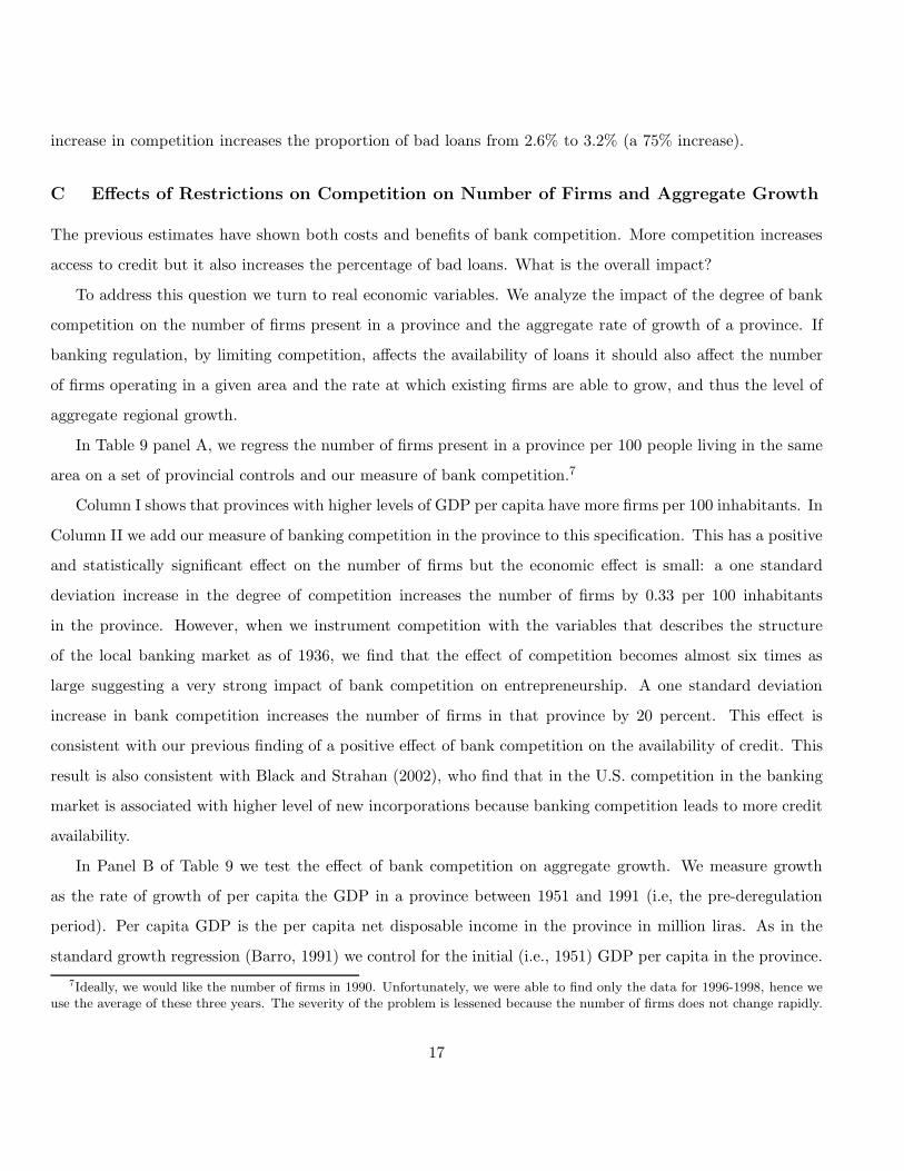
increase in competition increases the proportion of bad loans from 2.6% to 3.2% (a 75% increase).

C Effects of Restrictions on Competition on Number of Firms and Aggregate Growth

The previous estimates have shown both costs and benefits of bank competition. More competition increases

access to credit but it also increases the percentage of bad loans. What is the overall impact?

To address this question we turn to real economic variables. We analyze the impact of the degree of bank

competition on the number of firms present in a province and the aggregate rate of growth of a province. If

banking regulation, by limiting competition, affects the availability of loans it should also affect the number

of firms operating in a given area and the rate at which existing firms are able to grow, and thus the level of

aggregate regional growth.

In Table 9 panel A, we regress the number of firms present in a province per 100 people living in the same

area on a set of provincial controls and our measure of bank competition.7

Column I shows that provinces with higher levels of GDP per capita have more firms per 100 inhabitants. In

Column II we add our measure of banking competition in the province to this specification. This has a positive

and statistically significant effect on the number of firms but the economic effect is small: a one standard

deviation increase in the degree of competition increases the number of firms by 0.33 per 100 inhabitants

in the province. However, when we instrument competition with the variables that describes the structure

of the local banking market as of 1936, we find that the effect of competition becomes almost six times as

large suggesting a very strong impact of bank competition on entrepreneurship. A one standard deviation

increase in bank competition increases the number of firms in that province by 20 percent. This effect is

consistent with our previous finding of a positive effect of bank competition on the availability of credit. This

result is also consistent with Black and Strahan (2002), who find that in the U.S. competition in the banking

market is associated with higher level of new incorporations because banking competition leads to more credit

availability.

In Panel B of Table 9 we test the effect of bank competition on aggregate growth. We measure growth

as the rate of growth of per capita the GDP in a province between 1951 and 1991 (i.e, the pre-deregulation

period). Per capita GDP is the per capita net disposable income in the province in million liras. As in the

standard growth regression (Barro, 1991) we control for the initial (i.e., 1951) GDP per capita in the province.

7Ideally, we would like the number of firms in 1990. Unfortunately, we were able to find only the data for 1996-1998, hence weuse the average of these three years. The severity of the problem is lessened because the number of firms does not change rapidly.

17

In addition, we control for the preexisting level of infrastructure (defined as the sum of all the infrastructural

investments in the period 1936-1951 divided by the 1951 GDP per capita), and for the South dummy.

In column IV we insert, in addition to all these controls, our measure of bank competition. The coefficient

is positive, but it is not statistically significant. But if we instrument bank competition with our proxies for

exogenous restrictions on entry, we find that the degree of bank competition significantly affects GDP growth

rate of a province. Increasing competition by one standard deviation raises real economic growth by a quarter

of a percentage point per year. Almost half of the 60 basis points of difference in growth rate between the

Center-North and the South can be explained by the difference in the level of bank competition in these two

areas.

V How the Starting Level of Competition Affects the Impact of Deregu-

lation

By looking at the long-term effects of regulatory restrictions, in the previous section we have shown that

bank competition has positive economic effects, except for an increase in the percentage of bad loans. An

independent validation of the causal nature of this relationship comes from analyzing what happens when

these restrictions are removed. If the previously observed economic costs are really due to the lack of local

bank competition, after deregulation we should observe a catching up of those areas where the banking market

was less competitive during the regulation period.

This analysis of the effects of deregulation as a function of the pre-existing level of competition is interesting

also from another point of view. Many developing countries have liberalized their banking market without a

full understanding of what the cost and benefits of the transition are. This analysis can give us a sense of

these costs and benefits as a function of the starting conditions.

A Effects of Deregulation on the Supply of Loans

To study the effect of deregulation on the supply of credit to households, in Table 10a we pool the two

earliest surveys (1989 and 1991) with the two latest ones (1999-2001) and test the effect of the initial level of

competition on access to credit at a time of deregulation.

As Column I shows, deregulation brings a significant reduction in the number of households shut off from

18

the credit market (1.9% of all the households, equal to a reduction of 73% of the shut off households). Once

again, this effect cannot be attributed solely to deregulation because many other things change at the same

time. Nevertheless, it is hard to find any other plausible explanation for a reduction of this size.

As in Table 7a, households located in provinces with more bank competition are less likely to be shut off

from the credit market.

What Table 10a adds is that this effect disappears entirely after deregulation. Not only the coefficient of

the interaction between competition and deregulation is positive and statistically significant, but its magnitude

is almost exactly identical to the coefficient of competition alone. As expected, thus, deregulation makes all

local markets equally competitive, eliminating the effect of the initial conditions.

As column II shows, these results are robust to inserting a South dummy. Similarly, column III shows that

they are robust to instrumenting our measure of competition with the characteristics of the credit market in

1936.

In Table 10b we perform a similar type of analysis with the firms’ sample. We re-estimate the specification

in Table 7b pooling also the surveys after 1995 (de facto the surveys for the years 1998 and 2001).

As in Table 10a, we insert year dummies and an interaction between our measure of competition and a

liberalization dummy equal to 1 for the years 1998-2001. The pattern of the results is similar to the one

seen in Table 10a, but the effect is weaker. While the competition variable remains negative and statistically

significant and the interaction term is positive, the latter is not statistically significant and its size is an order

of magnitude smaller than the coefficient of competition alone.

One possible interpretation of these results is that there is not sufficient information in the data to estimate

precisely both effects given the size of the sample (each survey only includes 1,000 firms) and the small fraction

of rationed firms in normal times (around 2.5-3 percent). The pre-deregulation period includes the 1993-1995

recession when the share of rationed firms peaked to 13 percent, while there is no similar recession in the post

deregulation period. Hence, the higher magnitude of the coefficient and its statistical significance before but

not after might simply be due to this asymmetry in the data.

An alternative interpretation, however, is that the effect of deregulation is more immediate on household

credit than on business lending. This makes sense since it is much easier to create ex novo a consumer lending

department and find clients (given the high number of rationed households) than to initiate new relationship

with firms. The expertise associated to business lending is also more difficult to improvise.

19

If we accept this interpretation, this result carries an important implication for the effect of bank liber-

alization: consumer spending might react faster than business investments to the increased supply of credit.

This interpretation is consistent with Bayoumi (1993), who finds that consumption behavior is deeply affected

by financial liberalization in England in the 1980s.

B Effects of Deregulation on the Efficient Allocation of Credit

Table 6 showed that provinces with more bank competition experienced a higher fraction of bad loans during

the regulation period. How does the fraction of bad loan respond to the increase in competition generated by

deregulation? We look at this in Table 11. As a measure of the percentage of bad loans after deregulation we

use the average of 1999-2000 (the last year in our data). Our dependent variable is the difference between this

variable and the pre-deregulation level of bad loans, measured as in Table 6. For ease of reading, the difference

is multiplied by 100, so it is expressed in percentage points.

Interestingly, after deregulation the percentage of bad loans dropped, more in quantity (from 3.1% to 2.5%)

than in number (from 2.6 to 2.4%). We cannot, however, attribute this effect just to deregulation. Since, unlike

in Jayaratne and Strahan (1996), deregulation occurs simultaneously across the different provinces, we cannot

separate the effect of deregulation from other business cycle effects.

We can, however, study how this drop in percentage of bad loans relates to the initial level of competition

in the local banking market. This is what we do in Table 11. In the first column we show that the drop in

the percentage of bad loans is particularly pronounced in provinces that started the deregulation period more

competitive. One interpretation of this result is that local competition forced bank officers to be more skillful

in lending and this superior skill reduced the percentage of bad loans. Another interpretation is that in more

competitive areas, the percentage of bad loans was already high to begin with and so did not increase as much

(or decreased more) after deregulation.

If we look at the magnitude of the effect, however, the second explanation seems to be insufficient. During

regulation, a one standard deviation increase in competition increased the proportion of bad loans by 20 basis

points. After deregulation, a one standard deviation increase in the initial level of competition decreased the

proportion of bad loans by 54 basis points. Hence, the proportion of bad loans in non competitive areas not

only catches up to the level of competitive area, but exceeds it by 34 basis points. This suggests that lack of

competition has long lasting effect on banks’ ability to lend, which persist even after deregulation has taken

20

place.

As columns II and III suggest, the effect of the initial level of competition is not just a North-South effect

and it is not driven by differences in the GDP per capita. When we instrument competition with the structure

of the banking industry in 1936, the effect is much bigger in magnitude (one standard deviation increase in

competition decrease the proportion of bad loans by 134 basis points). The pattern is very similar if we use

the proportion of bad loans in terms of quantity rather than in terms of numbers (columns V to VIII).

C Effects of Deregulation on Number of Firms and Aggregate Growth

As for the level of regulation, we find that deregulation has both positive and negative effects: the supply of

loans increases but so does the percentage of bad loans. To assess the overall welfare effect we resort, once

again, to study the impact of deregulation on some real measures: the growth rate in the number of firms and

the aggregate growth rate.

In Table 12 panel A, we regress the number of new firms in a province per 100 people living in the same

area (average of 1996-98) on a set of provincial control and our measure of bank competition at the beginning

of deregulation.

Column I shows that provinces with higher levels of GDP per capita seem to have more creation of new

firms, but this effect is not statistically significant. Southern regions experience less firm creation. In Column

II we add our measure of banking competition in the province to this specification. This has a positive and

statistically significant effect on the creation of new firms after deregulation. This is somewhat surprising. We

would expect that the initial level of competition had no effect or even possibly a negative effect, since with

deregulation the other regions are catching up to the level of firm creation prevailing in the areas that started

more competitive. This effect persists when we instrument competition with the variables that describe the

structure of the local banking market as of 1936. Hence, it is not spurious.

While surprising, this result is consistent with our findings on the supply of credit. Deregulation does not

have an immediate impact on the supply of credit to firms and hence does not have an immediate impact on

the creation of new firms.

In Panel B of Table 12, we want to capture the effect of deregulation on the aggregate growth rate. If we

start from the standard growth regression used in Table 9b:

Growthit = α log(GDP ) it−1 + βCompetitionit + γSouthi + δIit + εit

21

where ”i” indexes the region and ”t” the time, then the effect of deregulation can be assessed by taking the

first difference between this equation before and after deregulation. Assuming that after deregulation all the

areas achieve a similar level of competition that we set equal to zero, and denoting Competitionib the index

of competition in region i before deregulation, we have

∆Growthit = α∆ log(GDP ) it−1 − βCompetitionib + δ∆Iit + ∆εit

Panel B of Table 12 runs this regression. We take the difference in the average growth rate after deregulation

(period 1991-1999) and the average growth rate before (period 1951 -1991). We regress this on the difference

in the log of the per capita GDP at the beginning of deregulation (1991) and the log of the per capita GDP at

the beginning gof the regulation period (1951). As we can see from column I, areas that started with a more

competitive banking sector grow relatively less during the deregulation period. Hence, deregulation allows less

competitive areas to catch up. This effect is present even if we control for the change in the initial level of

infrastructural investments (difference in infrastructural investment is the difference between the sum of all

the infrastructural investments before deregulation (1951-1991) divided by the 1991 GDP per capita and the

sum of all the infrastructural investments before the regulation period (1936-1951) divided by the 1951 GDP

per capita). The effect doubles in magnitude when we instrument our measure of competition with the 1936

banking structure variables.

Hence, while the effect of deregulation is not felt immediately on the entry of new firms, it is felt right

away on the growth rate.

VI Conclusions

In spite of the pervasiveness of bank regulation throughout the world, there is precious little evidence of its

welfare effects. By using some exogenous variation in the extent of restrictions on competition, this paper is

able to assess both the costs and benefits of regulation and the cost and benefits of deregulation.

We find that restrictions to competition reduce the supply of credit but also reduce the percentage of bad

loans. By contrast, deregulation increases the supply of credit and increases the percentage of bad loans.

Overall, restrictions on competition have negative effects on aggregate growth, effects that are undone when

bank regulation is lifted. We also find that in areas where competition was restricted, after deregulation the

percentage of bad loans raises above the level of competitive areas, suggesting that lack of competition has a

22

long lasting effect on a bank ability to grant credit in an efficient way.

23

References

[1] Albareto Giorgio and Maurizio Trapanese, 1999, “La politica bancaria negli anni cinquanta” Laterza,

Bari.

[2] Allen, Franklin and D. Gale, 2000, Comparing Financial Systems, M.I.T. Press, Cambridge MA.

[3] Allen, Franklin and D. Gale, 2004, “Competition and Financial Stability”, Journal of Money, Credit, and

Banking, Vol. 36, No. 3: 453-480.

[4] Allen N. Berger, Nathan H. Miller, Mitchell Petersen, Raghuram G. Rajan, and Jeremy C. Stein, 2005,

“Does Function Follow Organizational Form? Evidence From the Lending Practices of Large and Small

Banks,” Journal of Financial Economics, 76(2): 237-269

[5] Angelini P. and N. Cetorelli, 2003, “Bank Competition and Regulatory Reform: The Case of the Italian

Banking System,” Journal of Money Credit and Banking, 35, 663-684.

[6] Bank of Italy, 1977, Struttura Funzionale e territoriale del sistema bancario italiano, 1926-1974, Banca

D’Italia, Roma.

[7] Barth, James R., Gerard Caprio and Ross Levine, 2006, Rethinking Banking Regulation: till Angels

Govern, Cambridge University Press, Cambridge.

[8] Bayoumi, Tamin A., 1993, “Financial deregulation and consumption in the United Kingdom”, Review of

Economics and Statistics, 75(3):536-39.

[9] Beck, Thorsten, Norman Loayza and Ross Levine, 2000, “Finance and the Sources of Growth,” Journal

of Financial Economics, 58(1-2): 261-300.

[10] Beck, Thorsten, Asli Demirguc-Kunt and Ross Levine, 2006, “Bank Concentration, Competition, and

Crises: First Results,” Journal of Banking and Finance, 30(5): 1581-1603.

[11] Bekaert, Geert, C. Harvey, and Christian Lundblad, 2001, “Does Financial Liberalization Spur Growth,”

Duke University working paper.

[12] Bencivenga, Valerie and Bruce Smith, 1991, “Financial Intermediation and endogenous growth“, Review

of Economic Studies, 58(2), pp 195-209.

24

[13] Bernanke, Ben, 1983, “Non-Monetary Effects of the Financial Crisis in the Propagation of the Great

Depression,” American Economic Review, 73(3): 257-76.

[14] Bertrand, Marianne, Antoinette Schoar and Davif Thesmar, 2007, “Banking Deregulation and Industry

Structure: Evidence From the 1985 French Banking Reforms,” Journal of Finance, forthcoming

[15] Black Sandra and Philip Strahan, 2002, “Entrepreneurship and Bank Credit Availability,” Journal of

Finance, 57(6): 2807-33

[16] Bofondi, Marcello and Giorgio Gobbi , 2003, “Bad Loans and Entry in Local Credit Markets,” Bank of

Italy, Tema di discussione n. 509.

[17] Costi, Renzo, 2001, L’ordinamento bancario, Il Mulino, Bologna.

[18] Cotula, Franco and Juan Carlos Martizez Oliva, 2003, “Stabilit e sviluppo dalla liberazione al “miracolo

economico”,” in Franco Cotula, Marcello De Cecco and Gianni Toniolo (eds), 2003, La Banca dItalia.

Sintesi della ricerca storica 18931960, Laterza, Rome.

[19] De Cecco, Marcello, 1968, Saggi di Politica Monetaria, Giuffre, Milan.

[20] Dehejia, Rajeev and Adriana Lleras-Muney, 2005, “Financial Development and Pathways of Growth:

State Branching and Deposit Insurance Laws in the United States from 1900 to 1940,” Journal of Law

and Economics, forthcoming

[21] Demirguc, A. and V. Maksimovic, 1998, “Law, Finance, and Firm Growth,” Journal of Finance, 53,

2107-2138.

[22] Demirguc-Kunt, Aslı, Luc Laeven, and Ross Levine (2004) “Regulations, Market Structure, Institutions,

and the Cost of Financial Intermediation,” Journal of Money Credit and Banking, 36(3): 593-622

[23] Evans David S. and Boyan Jovanovic, 1989, “An Estimated Model of Entrepreneurial Choice under

Liquidity Constraints,” Journal of Political Economy ; 97(4): 808-27.

[24] Friedman, Thomas L., 1999, The Lexus and the Olive Tree: Understanding Globalization, New York :

Farrar, Straus & Giroux, 1999.

25

[25] Guiso, Luigi, Paola Sapienza, and Luigi Zingales, 2004, “Does Local Financial Development Matter?,”

Quarterly Journal of Economics, vol. 119 (3): 929-969

[26] Goldsmith, R., 1969, Financial Structure and Development, Yale University Press, New Haven.

[27] Gropp Reint, John Karl Scholz, and Michell J. White, 1997, “Personal Bankruptcy and Credit Supply

and Demand,” Quarterly Journal of Economics, 217-251.

[28] Holmstrom Bengt and Jean Tirole, 1997 “Financial Intermediation, Loanable Funds and the Real Sector,”

Quarterly Journal of Economics, 112(3): 663-691

[29] Holtz-Eakin, Douglas, David Joulfaian, and Harvey S. Rosen, 1994a, “Entrepreneurial Decisions and

Liquidity Constraints,” RAND Journal of Economics 23, 334-347.

[30] Holtz-Eakin, Douglas, David Joulfaian, and Harvey S. Rosen, 1994b, “Sticking it Out: Entrepreneurial

Survival and Liquidity Constraints,” Journal of Political Economy 102, 53-75.

[31] Higgins, 1977, “How much growth can a firm afford?” Financial Management, 6: 3-16.

[32] Jayaratne, Jith and Philip E. Strahan, 1996, “The Finance-Growth Nexus: Evidence from Bank Branch

Deregulation,” Quarterly Journal of Economics, CXI, 639-671.

[33] Levine, R., 1997, “Financial Development and Economic Growth: Views and Agenda,” Journal of Eco-

nomic Literature, 35: 688-726.

[34] Levine, R. And S. Zervos, 1998, “Stock Markets, Banks, and Economic Growth,” American Economic

Review, 88(3): 537-558.

[35] Lucas, Robert J. 1978, “On the Size Distribution of Business Firms,” Bell Journal of Economics, 9(2):

508-2.

[36] Petersen, Mitchell and Raghuram Rajan, 1995, “The Effect of Credit Market Competition on Lending

Relationships,” Quarterly Journal of Economics, 110 (2): 407-443.

[37] Petersen, Mitchell and Raghuram Rajan, 2002, “Does Distance Still Matter: The Information Revolution

in Small Business Lending,” Journal of Finance, 57, pp. 2533-2570.

26

[38] Polsi Alessandro (1996) “Financial institutions in nineteenth-century Italy. The rise of a banking system,”

Financial History Review, 3, October

[39] Polsi Alessandro (2000) “L’articolazione territoriale del sistema bancario italiano fra scelte di mercato e

intervento delle autorita monetarie,” in G. Conti and S. La Francesca Banche e reti di banche nell’Italia

Postunitaria, Il Mulino, Bologna

[40] Rajan, Raghuram and Luigi Zingales, 1998a, “Financial Dependence and Growth,” American Economic

Review, 88: 559-586.

[41] Rajan, Raghuram and Luigi Zingales, 1998b, “Which Capitalism? Lessons From the East Asia Crisis,”

Journal of Applied Corporate Finance, 11(3): 40-48.

[42] Rajan, R. and L. Zingales, 2001, “The Great Reversals: The Politics of Financial Development in the

20th Century,” Journal of Financial Economicsm 69(1), 5-50.

[43] Sapienza, Paola, 2004, “The Effects of Government Ownership on Bank Lending,” Journal of Financial

Economics, 72 (2): 357-384.

27

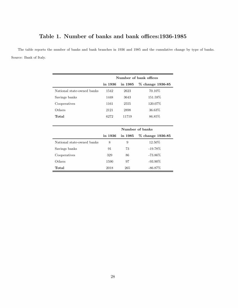
Table 1. Number of banks and bank offices:1936-1985

The table reports the number of banks and bank branches in 1936 and 1985 and the cumulative change by type of banks.

Source: Bank of Italy.

Number of bank offices

in 1936 in 1985 % change 1936-85

National state-owned banks 1542 2623 70.10%

Savings banks 1448 3643 151.59%

Cooperatives 1161 2555 120.07%

Others 2121 2898 36.63%

Total 6272 11719 86.85%

Number of banks

in 1936 in 1985 % change 1936-85

National state-owned banks 8 9 12.50%

Savings banks 91 73 -19.78%

Cooperatives 329 86 -73.86%

Others 1590 97 -93.90%

Total 2018 265 -86.87%

28

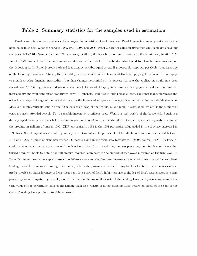
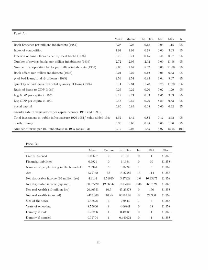
Table 2. Summary statistics for the samples used in estimation

Panel A reports summary statistics of the major characteristics of each province. Panel B reports summary statistics for the

households in the SHIW for the surveys 1989, 1991, 1998, and 2000. Panel C does the same for firms from SIM using data covering

the years 1998-2001. Sample for the SIM includes typically 1,000 firms but has been increasing I the latest year; in 2001 SIM

samples 2,793 firms. Panel D shows summary statistics for the matched firms-banks dataset used to estimate banks mark up on

the deposit rate. In Panel B credit rationed is a dummy variable equal to one if a household responds positively to at least one

of the following questions: “During the year did you or a member of the household think of applying for a loan or a mortgage

to a bank or other financial intermediary, but then changed your mind on the expectation that the application would have been

turned down?;” “During the year did you or a member of the household apply for a loan or a mortgage to a bank or other financial

intermediary and your application was turned down?.” Financial liabilities include personal loans, consumer loans, mortgages and

other loans. Age is the age of the household head in the household sample and the age of the individual in the individual sample.

Male is a dummy variable equal to one if the household head or the individual is a male. “Years of education” is the number of

years a person attended school. Net disposable income is in millions liras. Wealth is real wealth of the household. South is a

dummy equal to one if the household lives in a region south of Rome. Per capita GDP is the per capita net disposable income in

the province in millions of liras in 1990. GDP per capita in 1951 is the 1951 per capita value added in the province expressed in

1990 liras. Social capital is measured by average voter turnout at the province level for all the referenda on the period between

1946 and 1987. Number of firms present per 100 people living in the same area (average of 1996-98, source ISTAT). In Panel C

credit rationed is a dummy equal to one if the firm has applied for a loan during the year preceding the interview and was either

turned down or unable to obtain the full amount required; employees is the number of employees measured at the firm level. In

Panel D interest rate minus deposit rate is the difference between the firm level interest rate on credit lines charged by each bank

lending to the firm minus the average rate on deposits in the province were the lending bank is located; return on sales is firm

profits divides by sales; leverage is firms total debt as a share of firm’s liabilities; size is the log of firm’s assets; score is a firm

propensity score computed by the CB; size of the bank is the log of the assets of the lending bank; non performing loans is the

total value of non-performing loans of the lending bank as a %share of its outstanding loans; return on assets of the bank is the

share of lending bank profits to total bank assets.

29

Panel A:

Mean Median Std. Dev. Min Max N

Bank branches per millions inhabitants (1985) 0.28 0.26 0.18 0.04 1.15 95

Index of competition 1.91 1.94 0.75 0.00 3.63 95

Fraction of bank offices owned by local banks (1936) 0.76 0.74 0.15 0.46 0.97 95

Number of savings banks per million inhabitants (1936) 2.72 2.05 2.92 0.00 11.98 95

Number of cooperative banks per million inhabitants (1936) 8.60 7.57 5.62 0.00 21.66 95

Bank offices per million inhabitants (1936) 0.21 0.22 0.12 0.06 0.53 95

# of bad loans/total # of loans (1985) 2.59 2.51 0.83 1.04 5.07 95

Quantity of bad loans over total quantity of loans (1985) 3.14 2.81 1.78 0.78 11.28 95

Ratio of loans to GDP (1985) 0.27 0.22 0.20 0.02 1.29 95

Log GDP per capita in 1951 8.19 8.21 0.33 7.65 9.03 95

Log GDP per capita in 1991 9.43 9.52 0.26 8.89 9.83 95

Social capital 0.80 0.83 0.08 0.60 0.92 95

Growth rate in value added per capita between 1951 and 1999 (

Total investment in public infrastructure 1926-1951/ value added 1951 1.52 1.44 0.84 0.17 3.62 95

South dummy 0.36 0.00 0.48 0.00 1.00 95

Number of firms per 100 inhabitants in 1995 (obs=103) 9.19 9.03 1.55 5.97 13.55 103

Panel B:

Mean Median Std. Dev. 1st 99th Obs.

Credit rationed 0.02667 0 0.1611 0 1 31,358

Financial liabilities 0.6921 0 6.1384 0 10 31,358

Number of people living in the household 2.6946 3 1.35399 1 6 31,358

Age 53.2752 53 15.22586 16 114 31,358

Net disposable income (10 million lire) 4.3144 3.51645 3.47328 0.6 16.33377 31,358

Net disposable income (squared) 30.67722 12.36542 131.7036 0.36 266.7921 31,358

Net real wealth (10 million lire) 20.40553 10.5 45.23878 0 156 31,358

Net real wealth (squared) 2462.869 110.25 80197.08 0 24,336 31,358

Size of the town 2.47828 3 0.9843 1 4 31,358

Years of schooling 8.55606 8 4.66841 0 18 31,358

Dummy if male 0.76286 1 0.42533 0 1 31,358

Dummy if married 0.72794 1 0.445024 0 1 31,358

30

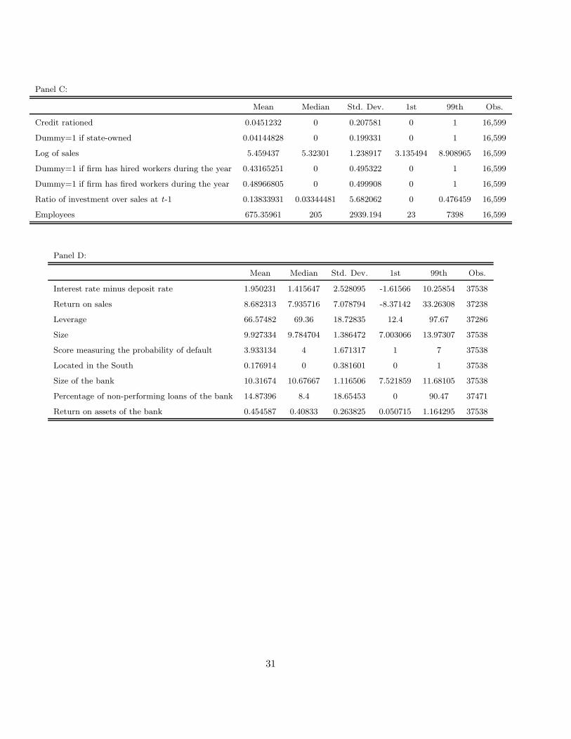
Panel C:

Mean Median Std. Dev. 1st 99th Obs.

Credit rationed 0.0451232 0 0.207581 0 1 16,599

Dummy=1 if state-owned 0.04144828 0 0.199331 0 1 16,599

Log of sales 5.459437 5.32301 1.238917 3.135494 8.908965 16,599

Dummy=1 if firm has hired workers during the year 0.43165251 0 0.495322 0 1 16,599

Dummy=1 if firm has fired workers during the year 0.48966805 0 0.499908 0 1 16,599

Ratio of investment over sales at t-1 0.13833931 0.03344481 5.682062 0 0.476459 16,599

Employees 675.35961 205 2939.194 23 7398 16,599

Panel D:

Mean Median Std. Dev. 1st 99th Obs.

Interest rate minus deposit rate 1.950231 1.415647 2.528095 -1.61566 10.25854 37538

Return on sales 8.682313 7.935716 7.078794 -8.37142 33.26308 37238

Leverage 66.57482 69.36 18.72835 12.4 97.67 37286

Size 9.927334 9.784704 1.386472 7.003066 13.97307 37538

Score measuring the probability of default 3.933134 4 1.671317 1 7 37538

Located in the South 0.176914 0 0.381601 0 1 37538

Size of the bank 10.31674 10.67667 1.116506 7.521859 11.68105 37538

Percentage of non-performing loans of the bank 14.87396 8.4 18.65453 0 90.47 37471

Return on assets of the bank 0.454587 0.40833 0.263825 0.050715 1.164295 37538

31

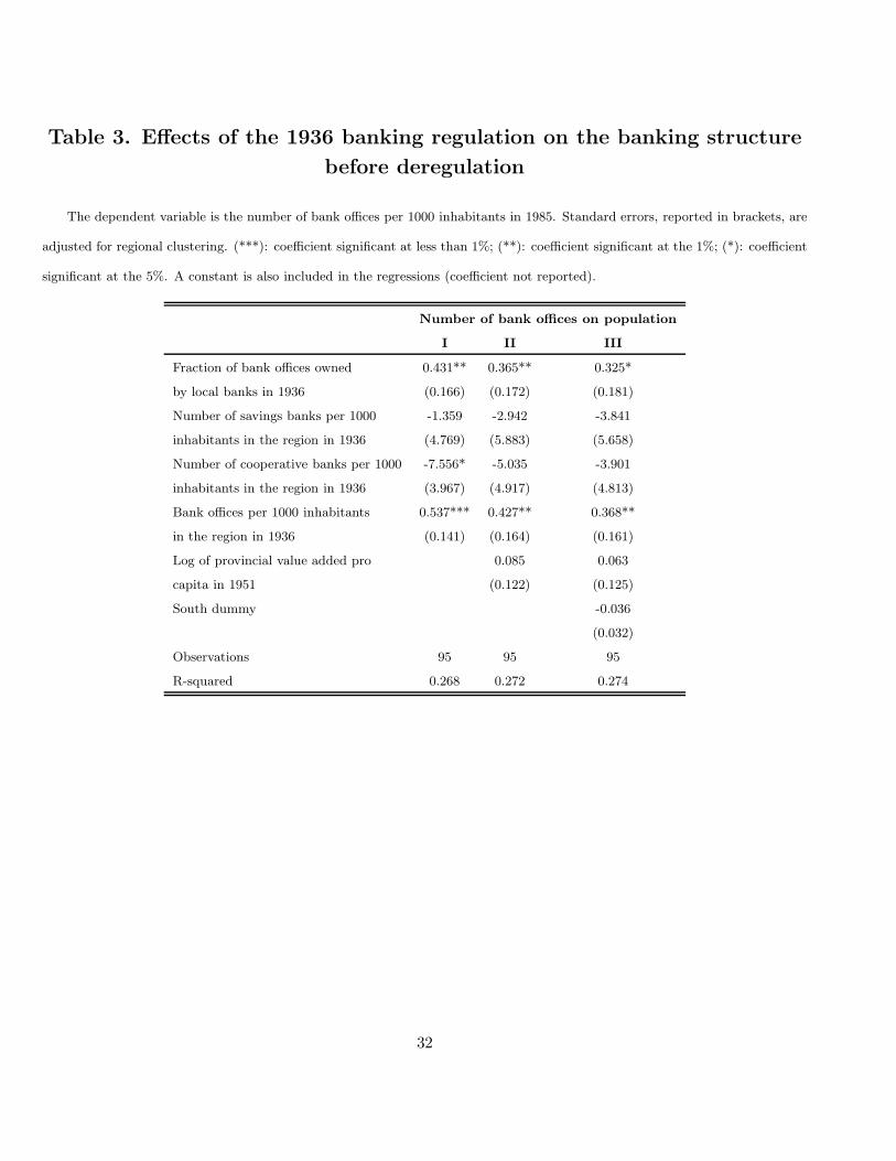
Table 3. Effects of the 1936 banking regulation on the banking structure

before deregulation

The dependent variable is the number of bank offices per 1000 inhabitants in 1985. Standard errors, reported in brackets, are

adjusted for regional clustering. (***): coefficient significant at less than 1%; (**): coefficient significant at the 1%; (*): coefficient

significant at the 5%. A constant is also included in the regressions (coefficient not reported).

Number of bank offices on population

I II III

Fraction of bank offices owned 0.431** 0.365** 0.325*

by local banks in 1936 (0.166) (0.172) (0.181)

Number of savings banks per 1000 -1.359 -2.942 -3.841

inhabitants in the region in 1936 (4.769) (5.883) (5.658)

Number of cooperative banks per 1000 -7.556* -5.035 -3.901

inhabitants in the region in 1936 (3.967) (4.917) (4.813)

Bank offices per 1000 inhabitants 0.537*** 0.427** 0.368**

in the region in 1936 (0.141) (0.164) (0.161)

Log of provincial value added pro 0.085 0.063

capita in 1951 (0.122) (0.125)

South dummy -0.036

(0.032)

Observations 95 95 95

R-squared 0.268 0.272 0.274

32

Table 4. Effects of the 1936 banking regulation on the level on interest

rates on firm loans before deregulation.

The table shows the effects of the 1936 banking structure on interest rates on loans charged to firms on credit lines before

deregulation. The data include a cross-section of bank-firm loan contracts for the year 1991. The dependent variable is the interest

rate charged to firm i by bank k at time t minus the prime rate at time t. Size of the firm is the logarithm of sales. We measure

the size of the bank by logarithm of total bank assets. The percentage of non-performing loans is a bank specific variable and it

calculated as the ratio of non-performing loans over total loans. Heteroscedasticity robust standard errors, reported in brackets, are

adjusted for regional clustering. (***): coefficient significant at less than 1%; (**): coefficient significant at the 1%; (*): coefficient

significant at the 5%.

33

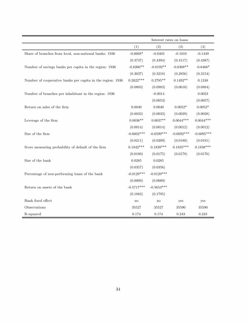
Interest rates on loans

(1) (2) (3) (4)

Share of branches from local, non-national banks: 1936 -0.6668* -0.6403 -0.1010 -0.1449

(0.3737) (0.4394) (0.4117) (0.4387)

Number of savings banks per capita in the region: 1936 -0.8266** -0.8192** -0.6308** -0.6466*

(0.3037) (0.3218) (0.2856) (0.3154)

Number of cooperative banks per capita in the region: 1936 0.2622*** 0.2785** 0.1492** 0.1248

(0.0803) (0.0983) (0.0616) (0.0884)

Number of branches per inhabitant in the region: 1936 -0.0014 0.0023

(0.0053) (0.0057)

Return on sales of the firm 0.0040 0.0040 0.0052* 0.0052*

(0.0033) (0.0033) (0.0029) (0.0028)

Leverage of the firm 0.0036** 0.0037** 0.0044*** 0.0044***

(0.0014) (0.0014) (0.0012) (0.0012)

Size of the firm -0.6602*** -0.6599*** -0.6092*** -0.6095***

(0.0211) (0.0209) (0.0180) (0.0181)

Score measuring probability of default of the firm 0.1842*** 0.1839*** 0.1835*** 0.1838***

(0.0180) (0.0175) (0.0178) (0.0176)

Size of the bank 0.0285 0.0285

(0.0357) (0.0356)

Percentage of non-performing loans of the bank -0.0129*** -0.0129***

(0.0009) (0.0009)

Return on assets of the bank -0.5717*** -0.5653***

(0.1882) (0.1795)

Bank fixed effect no no yes yes

Observations 35527 35527 35590 35590

R-squared 0.174 0.174 0.243 0.243

34

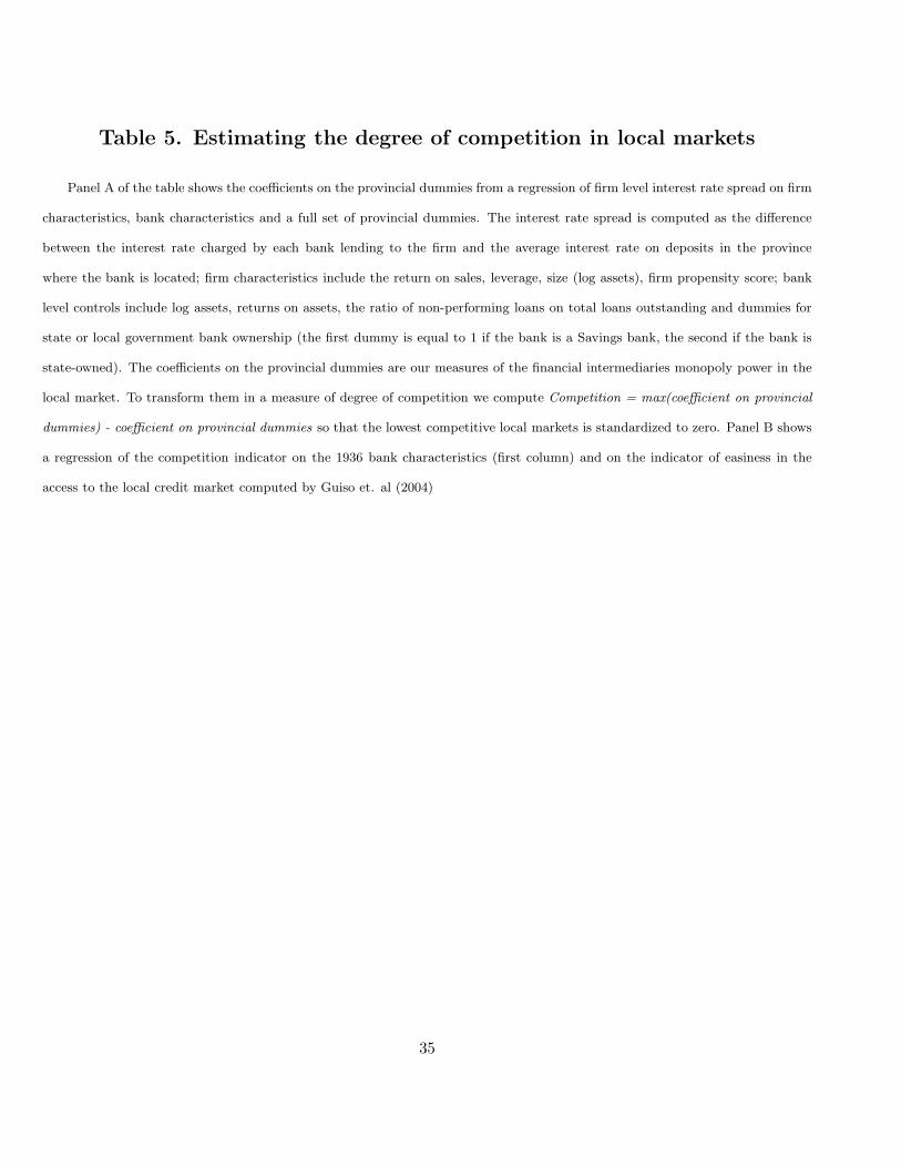
Table 5. Estimating the degree of competition in local markets

Panel A of the table shows the coefficients on the provincial dummies from a regression of firm level interest rate spread on firm

characteristics, bank characteristics and a full set of provincial dummies. The interest rate spread is computed as the difference

between the interest rate charged by each bank lending to the firm and the average interest rate on deposits in the province

where the bank is located; firm characteristics include the return on sales, leverage, size (log assets), firm propensity score; bank

level controls include log assets, returns on assets, the ratio of non-performing loans on total loans outstanding and dummies for

state or local government bank ownership (the first dummy is equal to 1 if the bank is a Savings bank, the second if the bank is

state-owned). The coefficients on the provincial dummies are our measures of the financial intermediaries monopoly power in the

local market. To transform them in a measure of degree of competition we compute Competition = max(coefficient on provincial

dummies) - coefficient on provincial dummies so that the lowest competitive local markets is standardized to zero. Panel B shows

a regression of the competition indicator on the 1936 bank characteristics (first column) and on the indicator of easiness in the

access to the local credit market computed by Guiso et. al (2004)

35

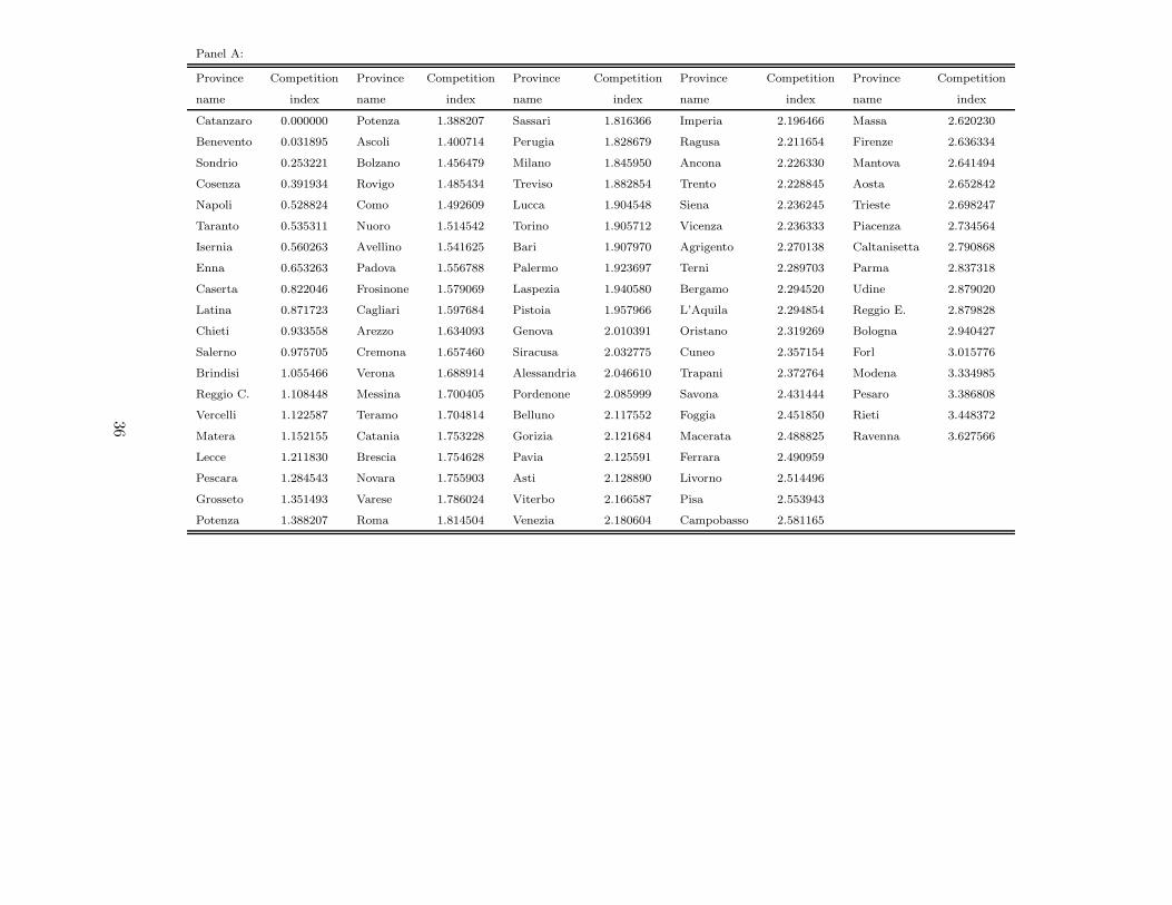
Panel A:

Province Competition Province Competition Province Competition Province Competition Province Competition

name index name index name index name index name index

Catanzaro 0.000000 Potenza 1.388207 Sassari 1.816366 Imperia 2.196466 Massa 2.620230

Benevento 0.031895 Ascoli 1.400714 Perugia 1.828679 Ragusa 2.211654 Firenze 2.636334

Sondrio 0.253221 Bolzano 1.456479 Milano 1.845950 Ancona 2.226330 Mantova 2.641494

Cosenza 0.391934 Rovigo 1.485434 Treviso 1.882854 Trento 2.228845 Aosta 2.652842

Napoli 0.528824 Como 1.492609 Lucca 1.904548 Siena 2.236245 Trieste 2.698247

Taranto 0.535311 Nuoro 1.514542 Torino 1.905712 Vicenza 2.236333 Piacenza 2.734564

Isernia 0.560263 Avellino 1.541625 Bari 1.907970 Agrigento 2.270138 Caltanisetta 2.790868

Enna 0.653263 Padova 1.556788 Palermo 1.923697 Terni 2.289703 Parma 2.837318

Caserta 0.822046 Frosinone 1.579069 Laspezia 1.940580 Bergamo 2.294520 Udine 2.879020

Latina 0.871723 Cagliari 1.597684 Pistoia 1.957966 L’Aquila 2.294854 Reggio E. 2.879828

Chieti 0.933558 Arezzo 1.634093 Genova 2.010391 Oristano 2.319269 Bologna 2.940427

Salerno 0.975705 Cremona 1.657460 Siracusa 2.032775 Cuneo 2.357154 Forl 3.015776

Brindisi 1.055466 Verona 1.688914 Alessandria 2.046610 Trapani 2.372764 Modena 3.334985

Reggio C. 1.108448 Messina 1.700405 Pordenone 2.085999 Savona 2.431444 Pesaro 3.386808

Vercelli 1.122587 Teramo 1.704814 Belluno 2.117552 Foggia 2.451850 Rieti 3.448372

Matera 1.152155 Catania 1.753228 Gorizia 2.121684 Macerata 2.488825 Ravenna 3.627566

Lecce 1.211830 Brescia 1.754628 Pavia 2.125591 Ferrara 2.490959

Pescara 1.284543 Novara 1.755903 Asti 2.128890 Livorno 2.514496

Grosseto 1.351493 Varese 1.786024 Viterbo 2.166587 Pisa 2.553943

Potenza 1.388207 Roma 1.814504 Venezia 2.180604 Campobasso 2.581165

36

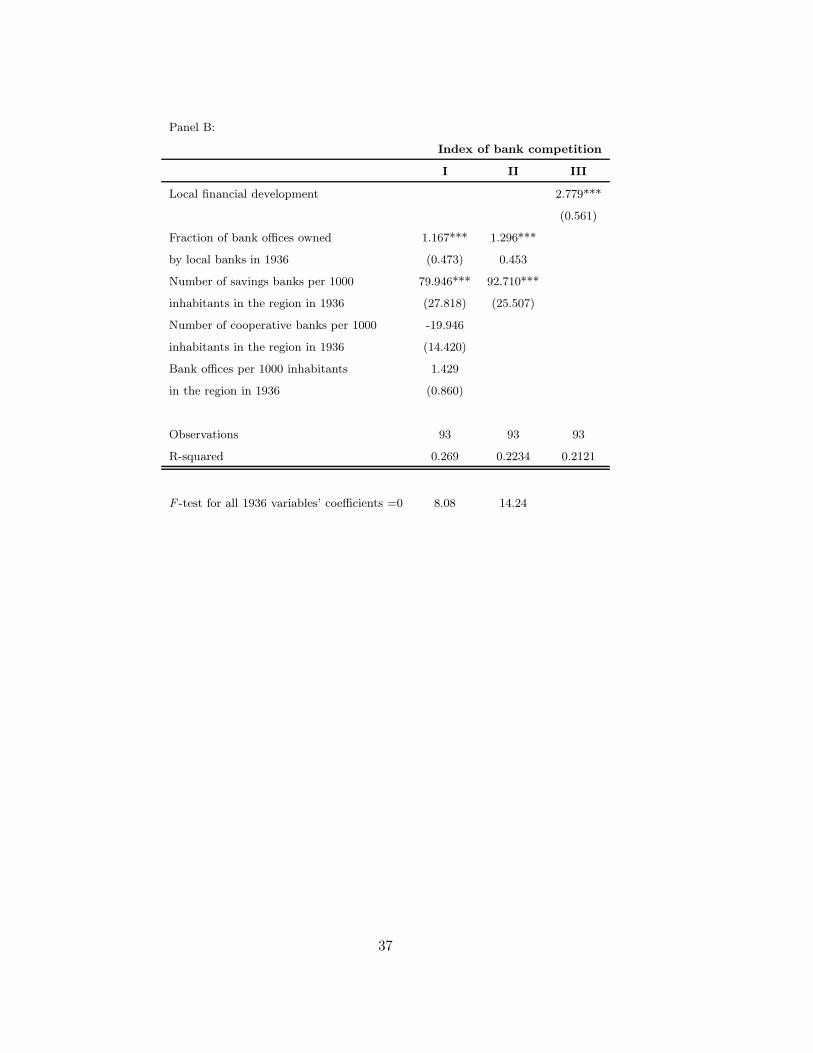
Panel B:

Index of bank competition

I II III

Local financial development 2.779***

(0.561)

Fraction of bank offices owned 1.167*** 1.296***

by local banks in 1936 (0.473) 0.453

Number of savings banks per 1000 79.946*** 92.710***

inhabitants in the region in 1936 (27.818) (25.507)

Number of cooperative banks per 1000 -19.946

inhabitants in the region in 1936 (14.420)

Bank offices per 1000 inhabitants 1.429

in the region in 1936 (0.860)

Observations 93 93 93

R-squared 0.269 0.2234 0.2121

F -test for all 1936 variables’ coefficients =0 8.08 14.24

37

Table 6. Effects of competition on the value of loans extended.

The table shows the effect of competition in the local credit market on the extension of loans prior to liberalization. The left

hand side is the value of loans extended scaled by value added in 1985. South is a dummy equal to one if the firm is located in

a region south of Rome. Competition is our measure of bank competition, based on interest rate spreads, derived in Table 5. IV

estimate use as instruments the 1936 measures of the structure of the banking system. Standard errors, reported in brackets, are

adjusted for regional clustering. (***): coefficient significant at less than 1%; (**): coefficient significant at the 1%; (*): coefficient

significant at the 5%. A constant is also included in the regressions (coefficient not reported).

Ratio of loans to value added

I II III IV

Competition in the local banking market 0.037** 0.008 -0.009 -0.161

(0.016) (0.020) (0.021) (0.098)

South dummy -0.101** 0.073 0.087

(0.043) (0.080) (0.089)

Log of provincial value added pro capita in 1981 0.382*** 0.633***

(0.131) (0.206)

Observations 95 95 95 95

R-squared 0.019 0.064 0.102

38

Table 7. Effect of competition on access to credit

In panel A the left hand side variable is a dummy equal to 1 if a household is credit constrained (i.e., declares it has been

turned down for a loan or discouraged from applying) and zero otherwise. The estimates include data from two SHIW surveys

prior to liberalization (1989-1991). Competition is our measure of bank competition, based on interest rate spreads, derived in

Table 5. In panel B the left hand side variable is a dummy equal to 1 if a firm is credit constrained (i.e., declares it has been turned

down for a loan or discouraged from applying) and zero otherwise. The estimates include observations from the surveys covering

the years 1988-1995. IV estimate use as instruments the 1936 measures of the structure of the banking system. Standard errors,

reported in brackets, are adjusted for regional clustering. (***): coefficient significant at less than 1%; (**): coefficient significant

at the 1%; (*): coefficient significant at the 5%.

39

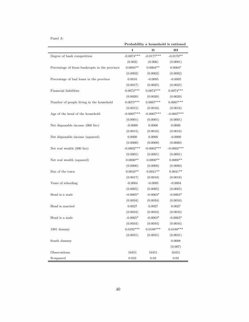
Panel A:

Probability a household is rationed

I II III

Degree of bank competition -0.0074*** -0.0177*** -0.0170**

(0.002) (0.006) (0.0081)

Percentage of firms bankrupts in the province 0.0004** 0.0004** 0.0004*

(0.0002) (0.0002) (0.0002)

Percentage of bad loans in the province 0.0016 -0.0005 -0.0005

(0.0017) (0.0025) (0.0025)

Financial liabilities 0.0073*** 0.0074*** 0.0074***

(0.0020) (0.0020) (0.0020)

Number of people living in the household 0.0075*** 0.0067*** 0.0067***

(0.0015) (0.0016) (0.0016)

Age of the head of the household -0.0007*** -0.0007*** -0.0007***

(0.0001) (0.0001) (0.0001)

Net disposable income (000 lire) -0.0000 0.0006 0.0006

(0.0015) (0.0016) (0.0016)

Net disposable income (squared) 0.0000 0.0000 -0.0000

(0.0000) (0.0000) (0.0000)

Net real wealth (000 lire) -0.0002*** -0.0002*** -0.0002***

(0.0001) (0.0001) (0.0001)

Net real wealth (squared) 0.0000** 0.0000** 0.0000**

(0.0000) (0.0000) (0.0000)

Size of the town 0.0043** 0.0041** 0.0041**

(0.0017) (0.0018) (0.0018)

Years of schooling -0.0004 -0.0005 -0.0004

(0.0005) (0.0005) (0.0005)

Head is a male -0.0065* -0.0063* -0.0063*

(0.0034) (0.0034) (0.0034)

Head is married 0.0027 0.0027 0.0027

(0.0034) (0.0034) (0.0034)

Head is a male -0.0065* -0.0063* -0.0063*

(0.0034) (0.0034) (0.0034)

1991 dummy 0.0192*** 0.0188*** 0.0188***

(0.0031) (0.0031) (0.0031)

South dummy 0.0008

(0.007)

Observations 16451 16451 16451

R-squared 0.022 0.02 0.02

40

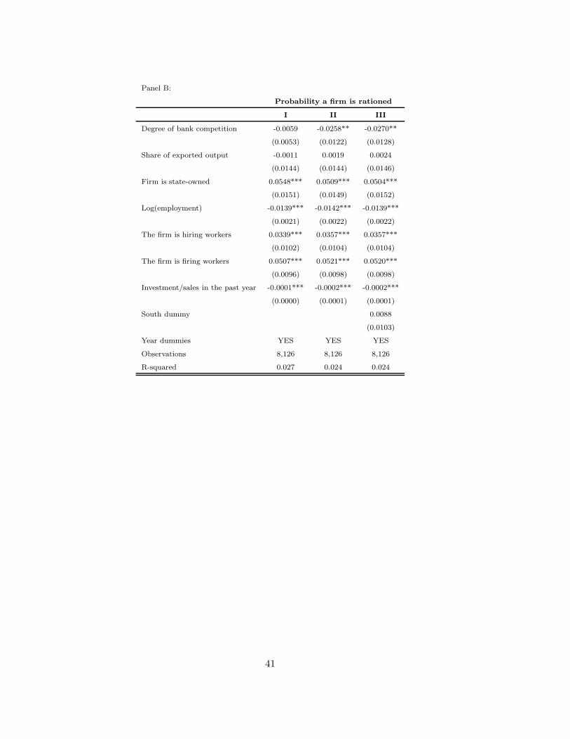
Panel B:

Probability a firm is rationed

I II III

Degree of bank competition -0.0059 -0.0258** -0.0270**

(0.0053) (0.0122) (0.0128)

Share of exported output -0.0011 0.0019 0.0024

(0.0144) (0.0144) (0.0146)

Firm is state-owned 0.0548*** 0.0509*** 0.0504***

(0.0151) (0.0149) (0.0152)

Log(employment) -0.0139*** -0.0142*** -0.0139***

(0.0021) (0.0022) (0.0022)

The firm is hiring workers 0.0339*** 0.0357*** 0.0357***

(0.0102) (0.0104) (0.0104)

The firm is firing workers 0.0507*** 0.0521*** 0.0520***

(0.0096) (0.0098) (0.0098)

Investment/sales in the past year -0.0001*** -0.0002*** -0.0002***

(0.0000) (0.0001) (0.0001)

South dummy 0.0088

(0.0103)

Year dummies YES YES YES

Observations 8,126 8,126 8,126

R-squared 0.027 0.024 0.024

41

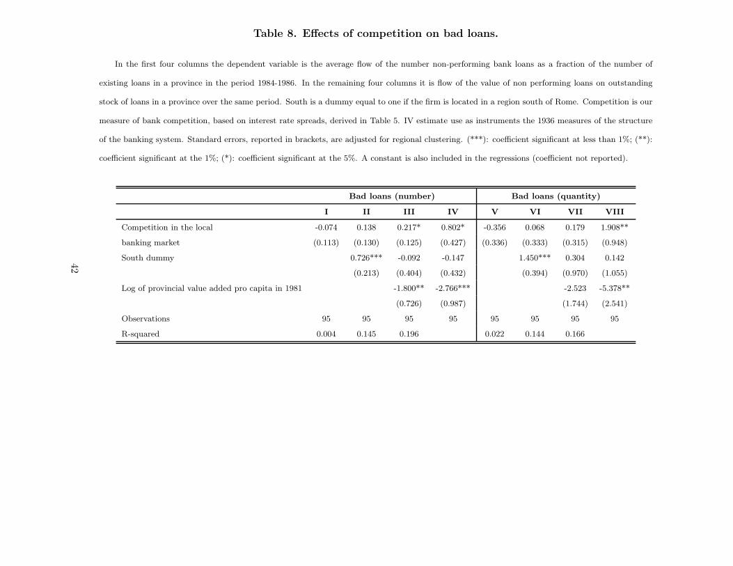
Table 8. Effects of competition on bad loans.

In the first four columns the dependent variable is the average flow of the number non-performing bank loans as a fraction of the number of

existing loans in a province in the period 1984-1986. In the remaining four columns it is flow of the value of non performing loans on outstanding

stock of loans in a province over the same period. South is a dummy equal to one if the firm is located in a region south of Rome. Competition is our

measure of bank competition, based on interest rate spreads, derived in Table 5. IV estimate use as instruments the 1936 measures of the structure

of the banking system. Standard errors, reported in brackets, are adjusted for regional clustering. (***): coefficient significant at less than 1%; (**):

coefficient significant at the 1%; (*): coefficient significant at the 5%. A constant is also included in the regressions (coefficient not reported).

Bad loans (number) Bad loans (quantity)

I II III IV V VI VII VIII

Competition in the local -0.074 0.138 0.217* 0.802* -0.356 0.068 0.179 1.908**

banking market (0.113) (0.130) (0.125) (0.427) (0.336) (0.333) (0.315) (0.948)

South dummy 0.726*** -0.092 -0.147 1.450*** 0.304 0.142

(0.213) (0.404) (0.432) (0.394) (0.970) (1.055)

Log of provincial value added pro capita in 1981 -1.800** -2.766*** -2.523 -5.378**

(0.726) (0.987) (1.744) (2.541)

Observations 95 95 95 95 95 95 95 95

R-squared 0.004 0.145 0.196 0.022 0.144 0.166

42

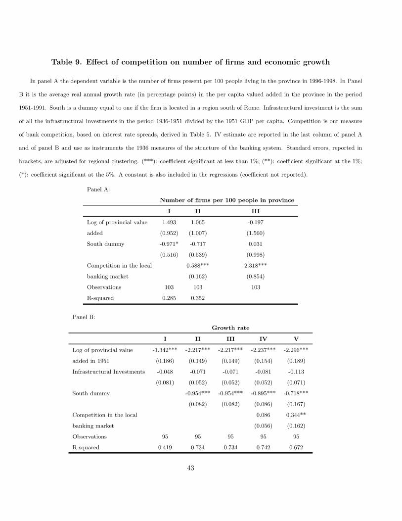
Table 9. Effect of competition on number of firms and economic growth

In panel A the dependent variable is the number of firms present per 100 people living in the province in 1996-1998. In Panel

B it is the average real annual growth rate (in percentage points) in the per capita valued added in the province in the period

1951-1991. South is a dummy equal to one if the firm is located in a region south of Rome. Infrastructural investment is the sum

of all the infrastructural investments in the period 1936-1951 divided by the 1951 GDP per capita. Competition is our measure

of bank competition, based on interest rate spreads, derived in Table 5. IV estimate are reported in the last column of panel A

and of panel B and use as instruments the 1936 measures of the structure of the banking system. Standard errors, reported in

brackets, are adjusted for regional clustering. (***): coefficient significant at less than 1%; (**): coefficient significant at the 1%;

(*): coefficient significant at the 5%. A constant is also included in the regressions (coefficient not reported).

Panel A:

Number of firms per 100 people in province

I II III

Log of provincial value 1.493 1.065 -0.197

added (0.952) (1.007) (1.560)

South dummy -0.971* -0.717 0.031

(0.516) (0.539) (0.998)

Competition in the local 0.588*** 2.318***

banking market (0.162) (0.854)

Observations 103 103 103

R-squared 0.285 0.352

Panel B:

Growth rate

I II III IV V

Log of provincial value -1.342*** -2.217*** -2.217*** -2.237*** -2.296***

added in 1951 (0.186) (0.149) (0.149) (0.154) (0.189)

Infrastructural Investments -0.048 -0.071 -0.071 -0.081 -0.113

(0.081) (0.052) (0.052) (0.052) (0.071)

South dummy -0.954*** -0.954*** -0.895*** -0.718***

(0.082) (0.082) (0.086) (0.167)

Competition in the local 0.086 0.344**

banking market (0.056) (0.162)

Observations 95 95 95 95 95

R-squared 0.419 0.734 0.734 0.742 0.672

43

Table 10. Effect of credit market liberalization on access to credit.

In panel A the left hand side variable is a dummy equal to 1 if a household is credit constrained (i.e., declares it has been turned

down for a loan or discouraged from applying) and zero otherwise. The estimates include data from two SHIW surveys both prior

to liberalization (1989-1991) and after liberalization (1998-2000). The number of observations in these regressions is slightly lower

than those shown in Table 2, panel B because the industry the household head works for is missing for some households. In panel

B the left hand side variable is a dummy equal to 1 if a firm is credit constrained (i.e., declares it has been turned down for a loan

or discouraged from applying) and zero otherwise. The estimates include observation both for the period prior to liberalization

(1988-1995) and after liberalization (1996-2001). The number of observations in these regressions is slightly lower than those shown

in Table 2, panel C because for some firms the location identifier is missing. IV estimate use as instruments the 1936 measures of

the structure of the banking system. Competition is our measure of bank competition, based on interest rate spreads, derived in

Table 5. Standard errors, reported in brackets, are adjusted for regional clustering. (***): coefficient significant at less than 1%;

(**): coefficient significant at the 1%; (*): coefficient significant at the 5%.

44

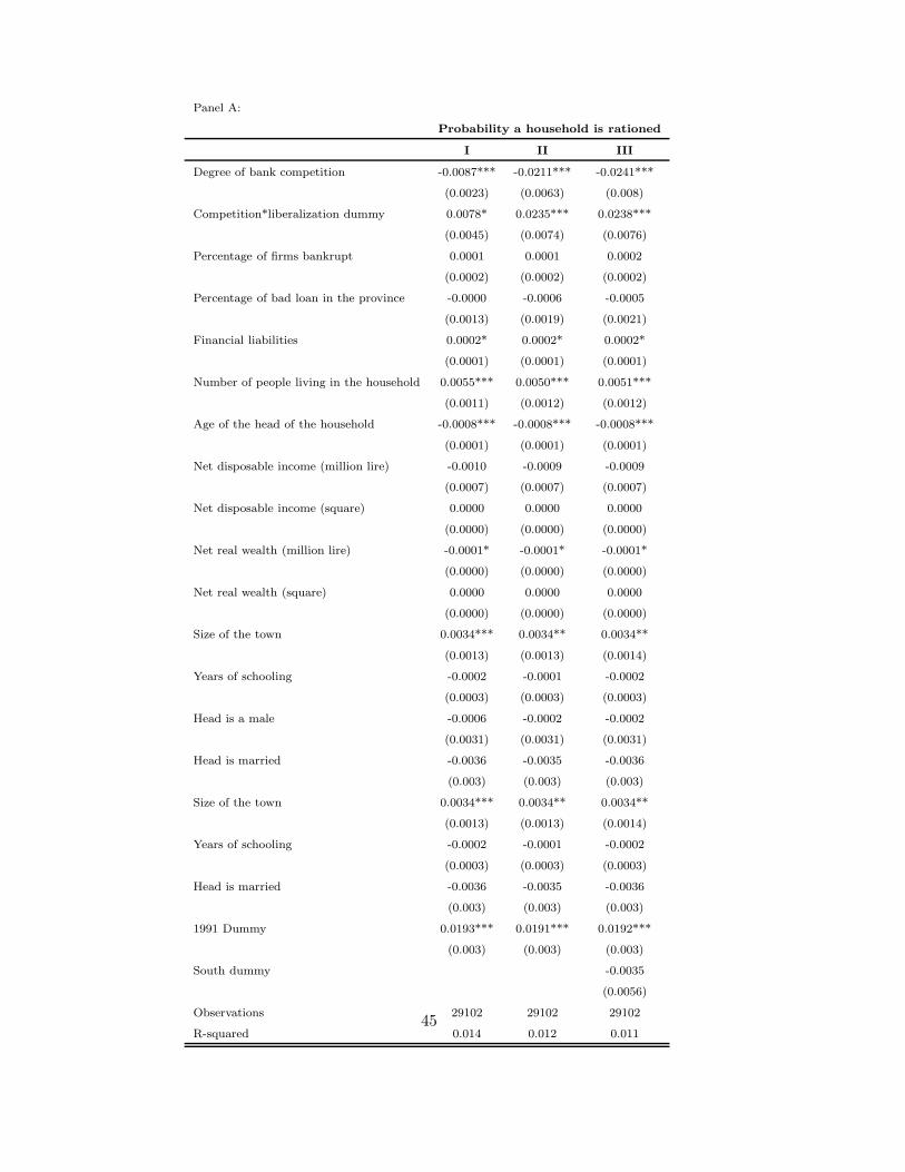
Panel A:

Probability a household is rationed

I II III

Degree of bank competition -0.0087*** -0.0211*** -0.0241***

(0.0023) (0.0063) (0.008)

Competition*liberalization dummy 0.0078* 0.0235*** 0.0238***

(0.0045) (0.0074) (0.0076)

Percentage of firms bankrupt 0.0001 0.0001 0.0002

(0.0002) (0.0002) (0.0002)

Percentage of bad loan in the province -0.0000 -0.0006 -0.0005

(0.0013) (0.0019) (0.0021)

Financial liabilities 0.0002* 0.0002* 0.0002*

(0.0001) (0.0001) (0.0001)

Number of people living in the household 0.0055*** 0.0050*** 0.0051***

(0.0011) (0.0012) (0.0012)

Age of the head of the household -0.0008*** -0.0008*** -0.0008***

(0.0001) (0.0001) (0.0001)

Net disposable income (million lire) -0.0010 -0.0009 -0.0009

(0.0007) (0.0007) (0.0007)

Net disposable income (square) 0.0000 0.0000 0.0000

(0.0000) (0.0000) (0.0000)

Net real wealth (million lire) -0.0001* -0.0001* -0.0001*

(0.0000) (0.0000) (0.0000)

Net real wealth (square) 0.0000 0.0000 0.0000

(0.0000) (0.0000) (0.0000)

Size of the town 0.0034*** 0.0034** 0.0034**

(0.0013) (0.0013) (0.0014)

Years of schooling -0.0002 -0.0001 -0.0002

(0.0003) (0.0003) (0.0003)

Head is a male -0.0006 -0.0002 -0.0002

(0.0031) (0.0031) (0.0031)

Head is married -0.0036 -0.0035 -0.0036

(0.003) (0.003) (0.003)

Size of the town 0.0034*** 0.0034** 0.0034**

(0.0013) (0.0013) (0.0014)

Years of schooling -0.0002 -0.0001 -0.0002

(0.0003) (0.0003) (0.0003)

Head is married -0.0036 -0.0035 -0.0036

(0.003) (0.003) (0.003)

1991 Dummy 0.0193*** 0.0191*** 0.0192***

(0.003) (0.003) (0.003)

South dummy -0.0035

(0.0056)

Observations 29102 29102 29102

R-squared 0.014 0.012 0.01145

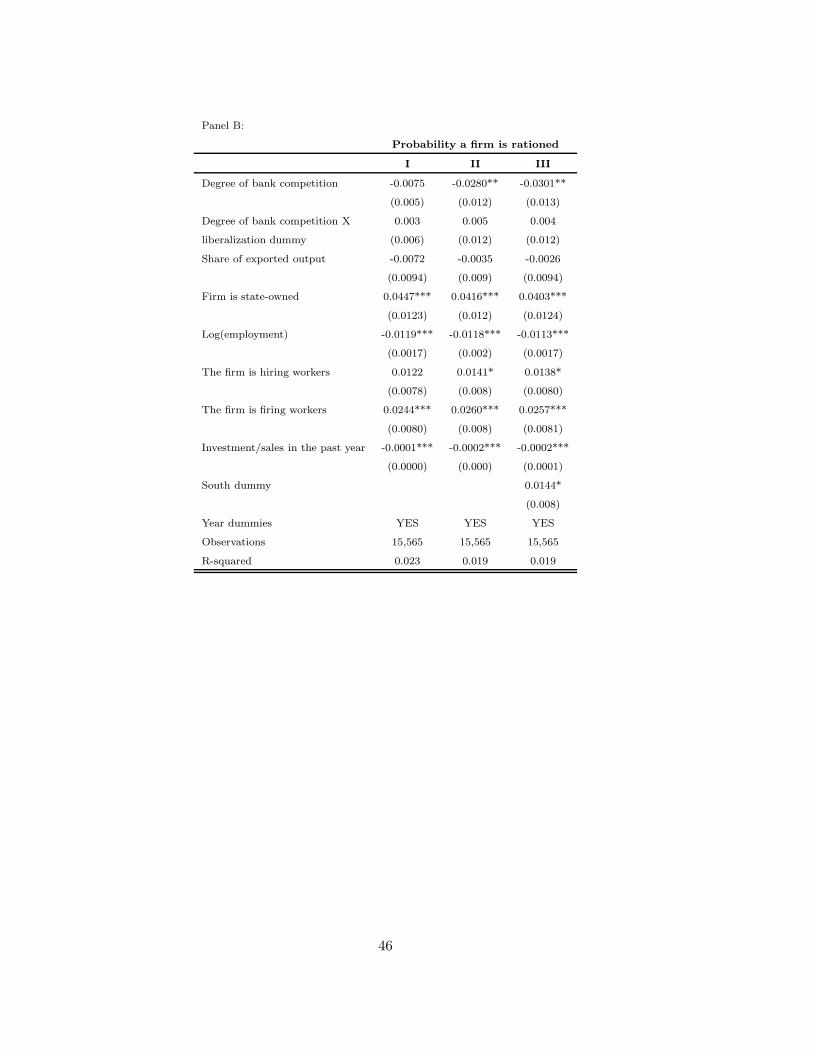
Panel B:

Probability a firm is rationed

I II III

Degree of bank competition -0.0075 -0.0280** -0.0301**

(0.005) (0.012) (0.013)

Degree of bank competition X 0.003 0.005 0.004

liberalization dummy (0.006) (0.012) (0.012)

Share of exported output -0.0072 -0.0035 -0.0026

(0.0094) (0.009) (0.0094)

Firm is state-owned 0.0447*** 0.0416*** 0.0403***

(0.0123) (0.012) (0.0124)

Log(employment) -0.0119*** -0.0118*** -0.0113***

(0.0017) (0.002) (0.0017)

The firm is hiring workers 0.0122 0.0141* 0.0138*

(0.0078) (0.008) (0.0080)

The firm is firing workers 0.0244*** 0.0260*** 0.0257***

(0.0080) (0.008) (0.0081)

Investment/sales in the past year -0.0001*** -0.0002*** -0.0002***

(0.0000) (0.000) (0.0001)

South dummy 0.0144*

(0.008)

Year dummies YES YES YES

Observations 15,565 15,565 15,565

R-squared 0.023 0.019 0.019

46

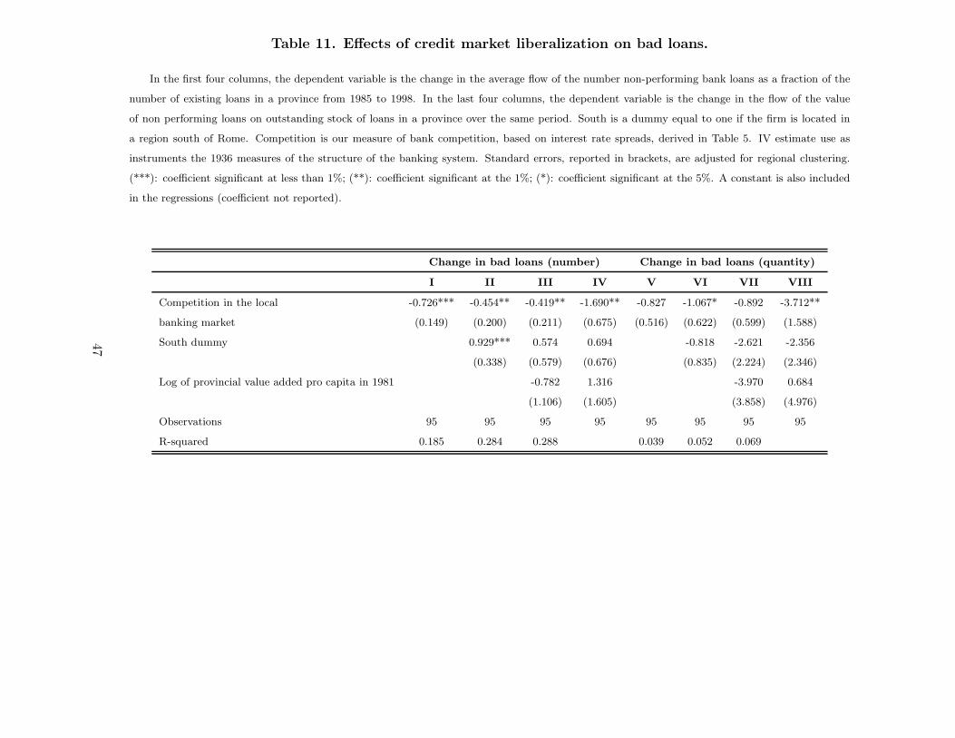
Table 11. Effects of credit market liberalization on bad loans.

In the first four columns, the dependent variable is the change in the average flow of the number non-performing bank loans as a fraction of the

number of existing loans in a province from 1985 to 1998. In the last four columns, the dependent variable is the change in the flow of the value

of non performing loans on outstanding stock of loans in a province over the same period. South is a dummy equal to one if the firm is located in

a region south of Rome. Competition is our measure of bank competition, based on interest rate spreads, derived in Table 5. IV estimate use as

instruments the 1936 measures of the structure of the banking system. Standard errors, reported in brackets, are adjusted for regional clustering.

(***): coefficient significant at less than 1%; (**): coefficient significant at the 1%; (*): coefficient significant at the 5%. A constant is also included

in the regressions (coefficient not reported).

Change in bad loans (number) Change in bad loans (quantity)

I II III IV V VI VII VIII

Competition in the local -0.726*** -0.454** -0.419** -1.690** -0.827 -1.067* -0.892 -3.712**

banking market (0.149) (0.200) (0.211) (0.675) (0.516) (0.622) (0.599) (1.588)

South dummy 0.929*** 0.574 0.694 -0.818 -2.621 -2.356

(0.338) (0.579) (0.676) (0.835) (2.224) (2.346)

Log of provincial value added pro capita in 1981 -0.782 1.316 -3.970 0.684

(1.106) (1.605) (3.858) (4.976)

Observations 95 95 95 95 95 95 95 95

R-squared 0.185 0.284 0.288 0.039 0.052 0.069

47

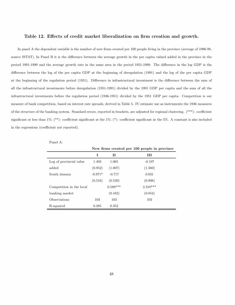
Table 12. Effects of credit market liberalization on firm creation and growth.

In panel A the dependent variable is the number of new firms created per 100 people living in the province (average of 1996-98,

source ISTAT). In Panel B it is the difference between the average growth in the per capita valued added in the province in the

period 1991-1999 and the average growth rate in the same area in the period 1951-1999. The difference in the log GDP is the

difference between the log of the per capita GDP at the beginning of deregulation (1991) and the log of the per capita GDP

at the beginning of the regulation period (1951). Difference in infrastructural investment is the difference between the sum of

all the infrastructural investments before deregulation (1951-1991) divided by the 1991 GDP per capita and the sum of all the

infrastructural investments before the regulation period (1936-1951) divided by the 1951 GDP per capita. Competition is our

measure of bank competition, based on interest rate spreads, derived in Table 5. IV estimate use as instruments the 1936 measures

of the structure of the banking system. Standard errors, reported in brackets, are adjusted for regional clustering. (***): coefficient

significant at less than 1%; (**): coefficient significant at the 1%; (*): coefficient significant at the 5%. A constant is also included

in the regressions (coefficient not reported).

Panel A:

New firms created per 100 people in province

I II III

Log of provincial value 1.493 1.065 -0.197

added (0.952) (1.007) (1.560)

South dummy -0.971* -0.717 0.031

(0.516) (0.539) (0.998)

Competition in the local 0.588*** 2.318***

banking market (0.162) (0.854)

Observations 103 103 103

R-squared 0.285 0.352

48

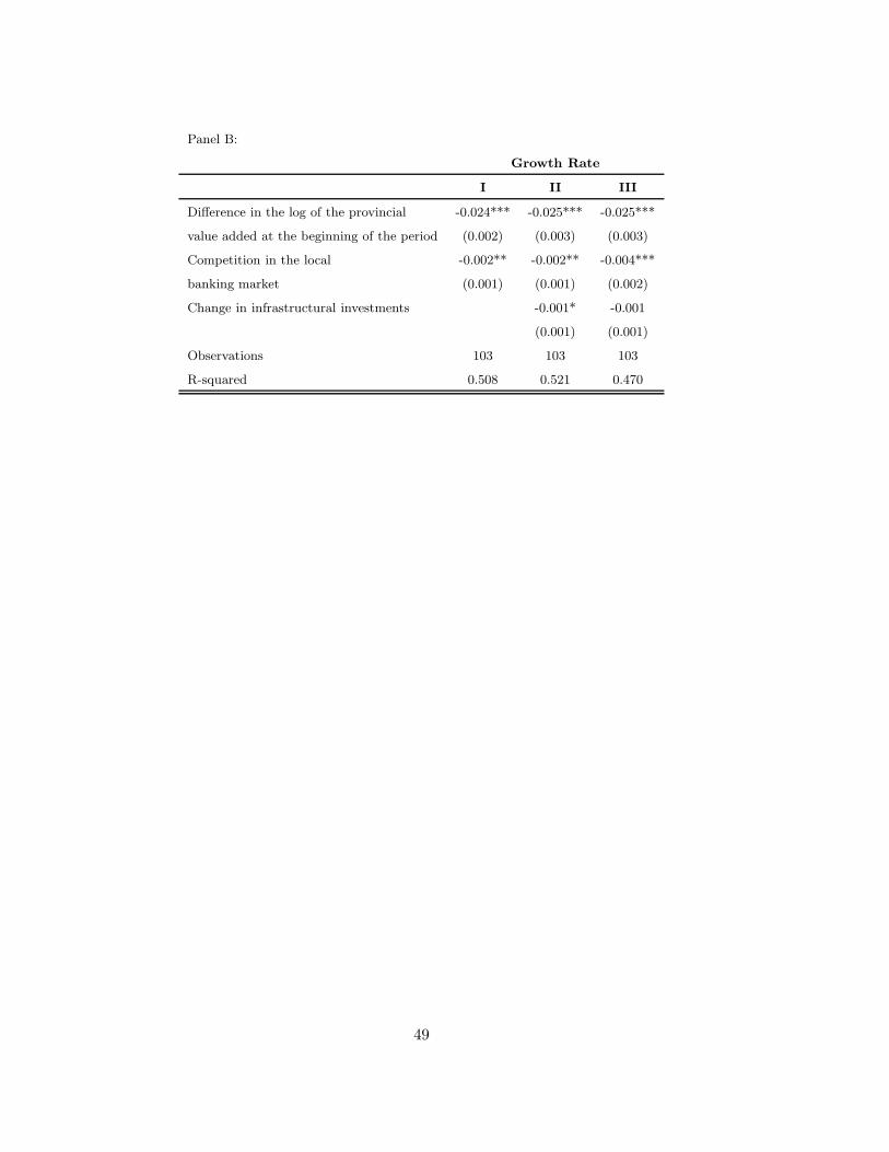
Panel B:

Growth Rate

I II III

Difference in the log of the provincial -0.024*** -0.025*** -0.025***

value added at the beginning of the period (0.002) (0.003) (0.003)

Competition in the local -0.002** -0.002** -0.004***

banking market (0.001) (0.001) (0.002)

Change in infrastructural investments -0.001* -0.001

(0.001) (0.001)

Observations 103 103 103

R-squared 0.508 0.521 0.470

49

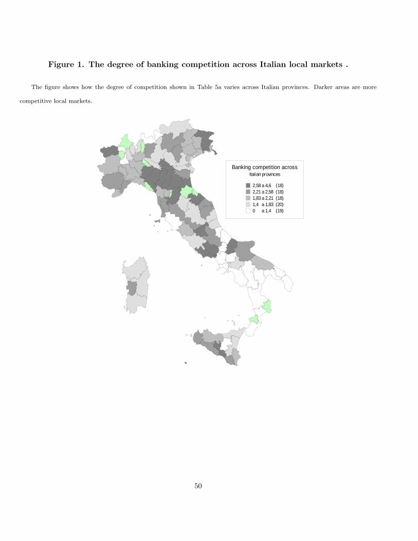
Figure 1. The degree of banking competition across Italian local markets .

The figure shows how the degree of competition shown in Table 5a varies across Italian provinces. Darker areas are more

competitive local markets.

Banking competition acrossItalian provinces

2,58 a 4,6 (18)2,21 a 2,58 (18)1,83 a 2,21 (18)1,4 a 1,83 (20)0 a 1,4 (19)

50