The Corpuscular Structure of Matter, the Interactions

1

The Corpuscular Structure of Matter, the Interactions between Particles, Quantum

Phenomena, and Cosmological Data as a Consequence of Selfvariations.

Emmanuil Manousos

APM Institute for the Advancement of Physics and Mathematics, 13 Pouliou str., 11 523

Athens, Greece

ABSTRACT

With the term “Law of Selfvariations” we mean an exactly determined increase of the

rest mass and the absolute value of the electric charge of material particles. In this article we

present the basic theoretical investigation of the law of selfvariations. We arrive at the central

conclusion that the interaction of material particles, the corpuscular structure of matter, and

the quantum phenomena can be justified by the law of Selfvariations. We predict a unified

interaction between particles with a unified mechanism (the Unified Selfvariation Interaction,

USVI). Every interaction is described by the three distinct terms with distinct consequences

in the USVI. The theory predicts a wave equation, whose special cases are the Maxwell

equations, the Schrödinger equation and the related wave equations. The theory provides a

mathematical expression for any conservable physical quantity, and the current density 4-

vector in every case. The corpuscular structure and wave behaviour of matter and the relation

between this emerge clearly and the theory also predicts the rest masses of material particles.

We prove an «internal symmetry» theorem which justifies the cosmological data. The study

we present can be the basis for further investigation of the theory and their consequences.

Keywords: Particles and Fields, Quantum Physics, Cosmology.

2

1. INTRODUCTION

The theoretical foundation of physics as developed in the last century, summed up

mainly in special and general theory of relativity and quantum mechanics. The great advances

in theoretical physics is mainly attributed to these two theories. There are however good

reasons to consider seriously that these two theories may not be the fundamental theories of

physics. The incompatibility between them, the failure to find a deeper cause of quantum

phenomena and the multiple assumptions, imposed by the experimental data, for the

development of quantum mechanics, are just some of these reasons.

These weaknesses of theoretical physics have led to build the confidence that the

deeper understanding of physical reality is impossible. Spearheading this argument was the

lack of understanding of quantum phenomena. Over the years Einstein's view that we should

seek and understand the cause of quantum phenomena was ignored and passed to the margin

A question that arises is whether there is a prominent fundamental law in nature. A

law which has the potential to reproduce our basic knowledge in physics. If indeed there is

such a law in nature then a continuing reduction of the axioms of theoretical physics is

expected to converge to this law. We present such a study below.

The present study is founded on three axioms: The principle of the conservation of the

four-vector of momentum, the equation of the Theory of Special Relativity for the rest mass

of the material particles and the law of Selfvariations.

With the term “Law of Selfvariations” we mean an exactly determined increase of the

rest mass and the absolute value of the electric charge of material particle. The law is

consistent with the principles of conservation of energy, momentum, angular momentum and

electric charge. It is also invariant under the Lorentz-Einstein transformations.

The most direct consequence of the law of Selfvariations is that energy, momentum,

angular momentum and electric charge (when the material particle is electrically charged) of

particles are distributed in the surrounding spacetime. For example, to compensate the

increase (in absolute value) of the electric charge of the electron, the particle emits a

corresponding positive electric charge into the surrounding spacetime. Otherwise, the

conservation of the electric charge is violated. Similarly, the increase of the rest mass of the

material particle involves the “emission” of negative energy as well as momentum in the

3

space-time surrounding the material particle (spacetime energy-momentum, STEM). Later

we will see that STEM contains charge in cose the particle is charged. The law of

Selfvariations quantitatively describes the interaction of material particles with the STEM.

Every material particle interacts both with the STEM emitted by itself due to the

selfvariations, and with the STEM originating from other material particles. The material

particle and the STEM with which it interacts, comprise a dynamic system which we called

“generalized particle”. In the present article we study this continuous interaction. The

conclusions resulting from the law of Selfvariations will be referred to as "the Theory of

Selfvariations" (TSV).

The main conclusion reached is that the three axioms we use reproduce all of our

basic knowledge in physics. In particular they predict and justify the particle structure of

matter, the interactions of particles, the quantum effects and the cosmological data. Moreover

an exceptionally large number of new statements about physical reality can be derived from

these axioms.

The TSV predicts a common mechanism for the interaction of particles which is the

Unified Selfvariation Interaction (USVI). The USVI implies that each interaction consists of

three components with different characteristics. One of these components corresponds to our

familiar Lorentz force as known from electromagnetism, one component corresponds to the

curvature of space-time, while the existence of the third component was totally unknown to

us before the formulation of the TSV.

The TSV predicts a wave equation whose special cases are the Maxwell's equations,

the Schrödinger equation and the associated wave equations. We determine a unified

mathematical expression for all conserved physical quantities and calculate the corresponding

4-vector for the current density. Both the density and the current density of conserved

physical quantities have a ‘crystalline’ structure which refers to the quantum behavior of

matter.

The equations of the TSV predict a strictly determined structure of matter. They

highlight both the particulate structure and the wave behavior of matter and the relationship

between them.

4

We prove a theorem, the internal symmetry theorem, which predicts and justifies the

cosmological data. We will show that for observations done at cosmological scale, our

observation instruments directly record the consequences of Selfvariations.

2. THE BASIC STUDY OF THE STRUCTURE OF THE GENERALIZED PARTICLE

2.1. Introduction

In this chapter we give the mathematical formulation of the law of selfvariations for

the rest mass and we determine the fundamental physical quantities , , 0,1,2,3ki k i which

are obtained from the law. For the formulation of the equations the following notation is

used:

W the energy of the particle

J the momentum of the particle

0m the rest mass of the particle

E the energy of the STEM interacting with the particle

P the momentum of the STEM interacting with the particle

0E the rest energy of the STEM interacting with the particle .

With the above symbolism, the law of Selfvariations for the rest mass is given by equations

00

0 0

m bEm

t

bm m

P

for 0 0m in every system of reference 0(t, , , )x y z , is the reduced Planck’s constant, b is

a constant, 0,b b and

x

y

z

.

5

The conclusions resulting from the law of Selfvariations will be referred to as "the

Theory of Selfvariations" (TSV). In the beginning we present the TSV in inertial frames of

reference.

2.2. The basic study of the internal structure of the generalized particle

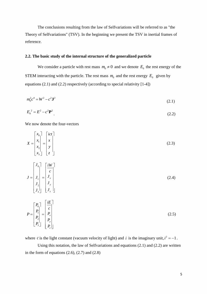
We consider a particle with rest mass 0 0m and we denote 0E the rest energy of the

STEM interacting with the particle. The rest mass 0m and the rest energy 0E given by

equations (2.1) and (2.2) respectively (according to special relativity [1-4])

2 4 2 2 2

0m c W c J (2.1)

2 2 2 2

0E E c P. (2.2)

We now denote the four-vectors

0

1

2

3

x ict

x xX

x y

zx

(2.3)

0

1

2

3

x

y

z

J iW

c

JJ J

JJ

JJ

(2.4)

0

1

2

3

x

y

z

iEP

cP

PPP

PP

P

(2.5)

where c is the light constant (vacuum velocity of light) and i is the imaginary unit, 2 1i .

Using this notation, the law of Selfvariations and equations (2.1) and (2.2) are written

in the form of equations (2.6), (2.7) and (2.8)

6

00 , 0,1,2,3k

k

m bP m k

x

,

0 0m (2.6)

2 2 2 2 2 2

0 1 2 3 0 0J J J J m c (2.7)

2

2 2 2 2 00 1 2 3 2

0.E

P P P Pc

(2.8)

However equations (2.7), (2.8) remain valid in the case where 0 0m ,

0 0E .

After differentiating equation (2.7) with respect to , 0,1,2,3kx k we obtain

20 3 01 2

0 1 2 3 0 0k k k k k

J J mJ JJ J J J m c

x x x x x

and with equation (2.6) we obtain

2 20 31 2

0 1 2 3 0 0k

k k k k

J JJ J bJ J J J P m c

x x x x


2 2 2 20 31 20 1 2 3 0 1 2 3 0k

k k k k

J JJ J bJ J J J P J J J J

x x x x

0 10 0 1 1

322 2 3 3 0, 0,1,2,3

k k

k k

k k

k k

J Jb bJ P J J P J

x x

JJ b bJ P J J P J k

x x

. (2.9)

We now symbolize

, , 0,1,2,3ik i ki

k

J bP J k i

x

. (2.10)

With this notation, equation (2.9) can be written in the form

0 0 1 1 2 2 3 3 0, 0,1,2,3k k k kJ J J J k . (2.11)

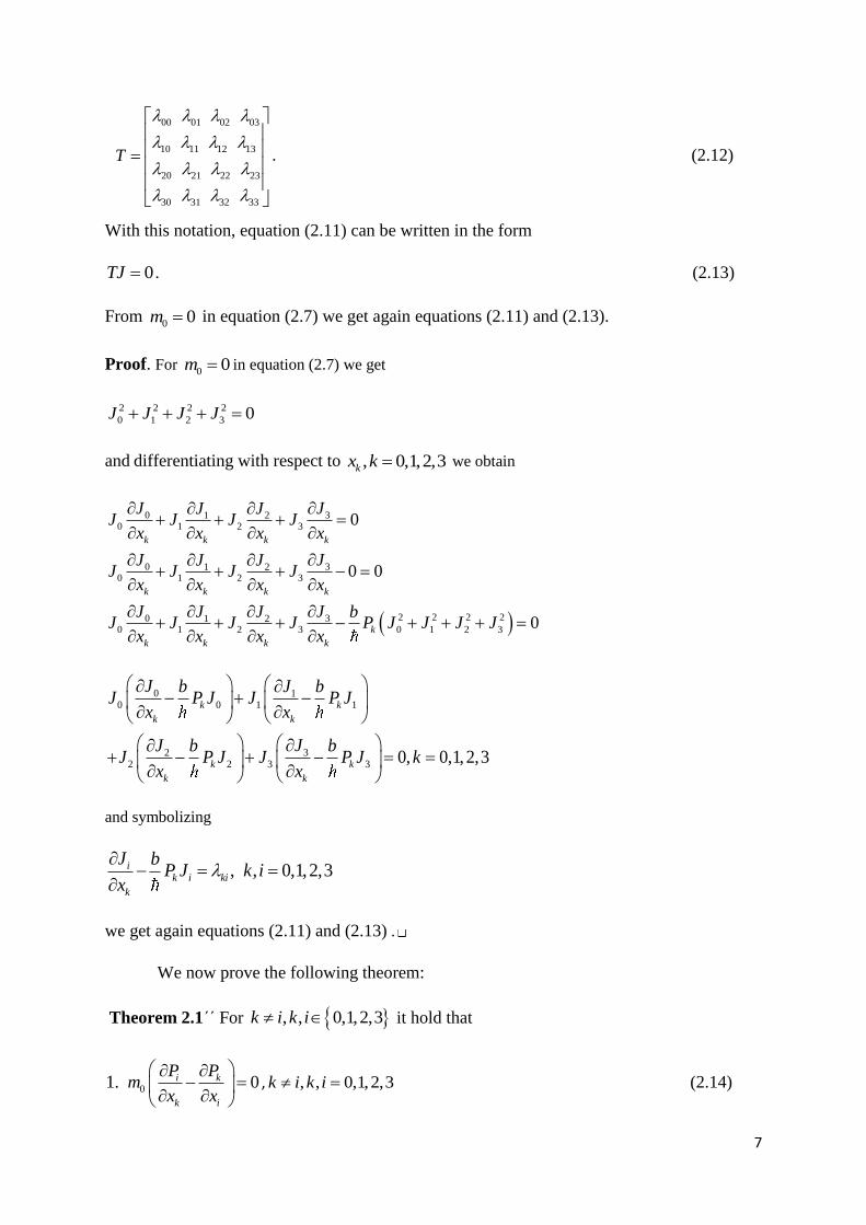
We now need the 4 4 matrix T as given by equation

7

00 01 02 03

10 11 12 13

20 21 22 23

30 31 32 33

T

. (2.12)

With this notation, equation (2.11) can be written in the form

0TJ . (2.13)

From 0 0m in equation (2.7) we get again equations (2.11) and (2.13).

Proof. For 0 0m in equation (2.7) we get

2 2 2 2

0 1 2 3 0J J J J

and differentiating with respect to , 0,1,2,3kx k we obtain

0 31 20 1 2 3

0 31 20 1 2 3

2 2 2 20 31 20 1 2 3 0 1 2 3

0

0 0

0

k k k k

k k k k

k

k k k k

J JJ JJ J J J

x x x x

J JJ JJ J J J

x x x x

J JJ J bJ J J J P J J J J

x x x x

0 10 0 1 1

322 2 3 3 0, 0,1,2,3

k k

k k

k k

k k

J Jb bJ P J J P J

x x

JJ b bJ P J J P J k

x x

and symbolizing

, , 0,1,2,3ik i ki

k

J bP J k i

x

we get again equations (2.11) and (2.13) .

We now prove the following theorem:

Theorem 2.1΄΄ For , , 0,1,2,3k i k i it hold that

1. 0 0i k

k i

P Pm

x x

, , , 0,1,2,3k i k i (2.14)

8

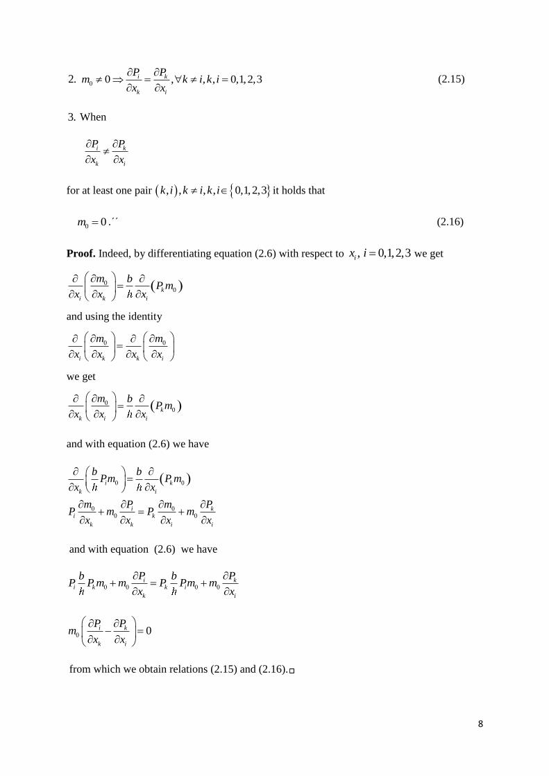
2. 0 0 , , , 0,1,2,3i k

k i

P Pm k i k i

x x

(2.15)

3. When

i k

k i

P P

x x

for at least one pair , , , , 0,1,2,3k i k i k i it holds that

0 0m .΄΄ (2.16)

Proof. Indeed, by differentiating equation (2.6) with respect to , 0,1,2,3ix i we get

00k

i k i

m bP m

x x x

and using the identity

0 0

i k k i

m m

x x x x

we get

00k

k i i

m bP m

x x x

and with equation (2.6) we have

0 0

0 00 0

i k

k i

i ki k

k k i i

b bPm P m

x x

m P m PP m P m

x x x x


0 0 0 0i k

i k k i

k i

P Pb bP P m m P Pm m

x x

0 0i k

k i

P Pm

x x

from which we obtain relations (2.15) and (2.16).

9

3. PHYSICAL QUANTITIES kiλ , k,i = 0,1,2,3 AND THE CONSERVATION

PRINCIPLES OF ENERGY AND MOMENTUM

3.1. Introduction

The physical quantities , , 0,1,2,3ki k i are related to the conservation of energy and

momentum of the generalized particle. This investigation we will present in this section.

We present the internal symmetry, which expresses the isotropy of spacetime, and

the external symmetry which expresses the anisotropy of spacetime. In this chapter we two of

the fundamental theorems of TSV: the theorem of internal symmetry and the first theorem of

external symmetry.

3.2. Physical quantities kiλ , k,i = 0,1,2,3 and the conservation principles of energy and

momentum

We start our study with the proof of the following theorem:

Theorem 3.1 ΄΄For 0 0m and when the generalized particle conserves its momentum along

the axes , 0,1,2,3ix i , that is

constanti i iJ P c (3.1)

then the following equation holds

ki ik k i i k i k k i k i i k

b b bJ P J P c J c J c P c P (3.2)

for every , 0,1,2,3, .k i k i ΄΄

Proof. Combining relation (2.15) with equation (3.1) we obtain

i i k k

k i

c J c Jx x

i k

k i

J J

x x

10

and with equation (2.10) we get

k i ki i k ik

ki ik k i i k

b bP J PJ

bJ P J P

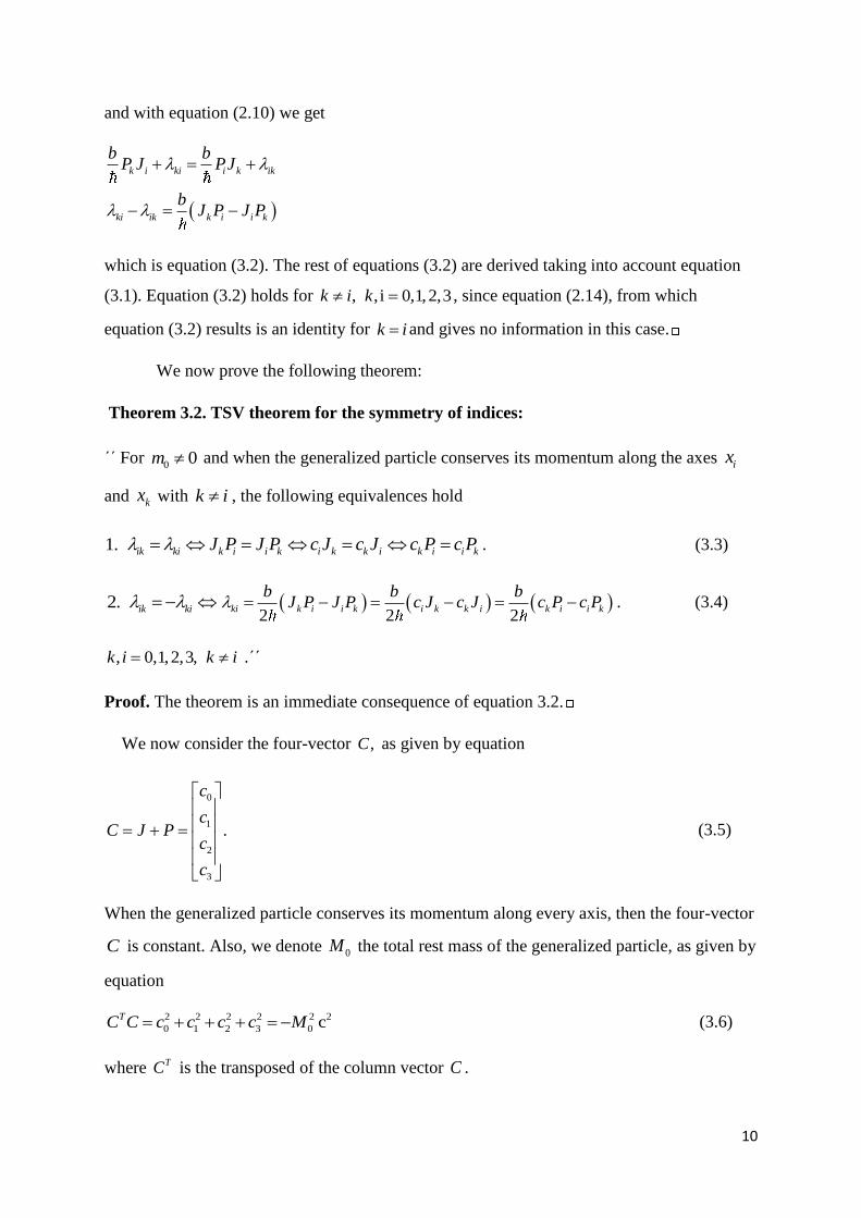
which is equation (3.2). The rest of equations (3.2) are derived taking into account equation

(3.1). Equation (3.2) holds for , , i 0,1,2,3k i k , since equation (2.14), from which

equation (3.2) results is an identity for k i and gives no information in this case.


Theorem 3.2. TSV theorem for the symmetry of indices:

΄΄ For 0 0m and when the generalized particle conserves its momentum along the axes ix

and kx with k i , the following equivalences hold

1. ik ki k i i k i k k i k i i kJ P J P c J c J c P c P . (3.3)

2. ik ki 2 2 2

ki k i i k i k k i k i i k

b b bJ P J P c J c J c P c P . (3.4)

, 0,1,2,3,k i k i .΄΄

Proof. The theorem is an immediate consequence of equation 3.2.

We now consider the four-vector ,C as given by equation

0

1

2

3

.

c

cC J P

c

c

(3.5)

When the generalized particle conserves its momentum along every axis, then the four-vector

C is constant. Also, we denote 0M the total rest mass of the generalized particle, as given by

equation

2 2 2 2 2 2

0 1 2 3 0 cTC C c c c c M (3.6)

where TC is the transposed of the column vector C .

11

For reasons that will become apparent later in our study, we give the following

definitions: We name the symmetry , , , 0,1,2,3ik ki k i k i internal symmetry, and the

symmetry , , , 0,1,2,3ik ki k i k i external symmetry. We now prove the following

theorem:

Theorem 3.3. Internal Symmetry Theorem:

΄΄ For 0 0m and when the generalized particle conserves its momentum in every axis, the

following hold:

1. ik ki for every , 0,1,2,3k i J , P and C are parallel

P J where . (3.7)

2. For 1 or 0 the following equations hold

2

0 0 0

0 0 0

0

0

E m c M

m M E

(3.8)

respectively.

3. For 1 and 0 the following equations hold:

0 0 1 1 2 2 3 3expb

K c x c x c x c x

(3.9)

00

1

Mm

(3.10)

2

00

1

M cE

(3.11)

, 0,1,2,31

ii

cJ i

(3.12)

, i 0,1,2,31

ii

cP

(3.13)

where K is a dimensionless constant physical quantity.

We have ik ki for every , i 0,1,2,3k

(3.14)

0ki for every , i 0,1,2,3k . ΄΄

12

Proof. Equivalence (3.7) result immediately from equivalence (3.3). For 1 from the

last of equivalence (3.7) we obtain P J and from equations (2.7), (2.8) and (3.5), (3.6) we

obtain

2 2 2

0 0 0 0E m c M

which is the first of the equations (3.8). For 0 from the last of equivalence (3.7) we

obtain 0P and from equations (3.5), (3.6) and (2.7) we obtain

2 2

0 0 0 0m M E

which is the second of the equations (3.8).

For 1 and 0 from the last of equivalence (3.7) we obtain i iP J for

every 0,1,2,3i and with equation (3.1) i i iJ P c we initially obtain equations (3.12) and

(3.13). Then, combining equations (2.7) and (3.12) we get

2 2 2 2 2 2

0 0 1 2 32

10

1m c c c c c

and with equation (3.6) we obtain equation

2 22 2 00 2

01

M cm c

(3.15)

and we finally have

00

1

Mm

which is equation (3.10). Similarly, combining equations (2.8) and (3.13) we obtain equation

(3.11). We now prove that function is given by equation (3.9).

Differentiating equation (3.15) with respect to , 0,1,2,3vx v and considering

equation (2.6) we obtain

2 22 2 00 3

220

1v

v

M cbPm c

x


13

2 2 2 2

0 0

2 30

1 1

1

v

v

v

v

M c M cbP

x

bP

x

and with equation (3.13) for i v we arrive at equation

, 0,1,2,3.v

v

bc v

x

(3.16)

By integration of equation (3.16) we obtain

0 0 1 1 2 2 3 3expb

K c x c x c x c x

where K is the integration constant, which is equation (3.9).

Combining equations (2.10), (3.12) and (3.13) for 0,1,2,3k we obtain

iki k i

k

J bP J

x

1 1 1

i k iki

k

c c cb

x

2 21 1

i k iki

k

c c cb

x

and with equation (3.16) for k we obtain

2 2

1 1

i k iki k

c c cb bc

0ki .

We formulated internal symmetry theorem for 0J in order for the material particle

to exist. If we formulate the theorem for 0P , the material particle and the STEM exchange

places in the equations and the conclusions of the TSV.

Following we do the study based on case 3. of the internal symmetry theorem. That is

in the case where 1 and 0 . The study of the cases 1 and 0 , i.e. of eqs.

(3.8) are not considered in the present publication.

14

According to the previous theorem, internal symmetry is equivalent to the parallelism

of the four-vectors ,J P . Starting from this conclusion we can determine the physical content

of the internal symmetry.

In an isotropic space the spontaneous emission of STEM by the material particle is

isotropic. Due to the linearity of the Lorentz-Einstein transformations, this isotropic emission

has as a consequence the parallelism of the four-vectors ,J P ([5] par. 5.3). Thus, the

theorem of internal symmetry 3.3 holds for the spontaneous emission of STEM by the

material particle due to Selfvariations .

In the following chapters, we will make clear that the internal symmetry refers to a

spontaneous internal increase of the rest mass and the electrical charge of the material

particles, independent of any external causes. The consequences of this increase is the

cosmological data, as we'll see in Chapter 16. Also, the internal symmetry is associated with

Heisenberg's uncertainty principle.

We start the investigation of the external symmetry with the proof of the following

theorem:

Theorem 3.4. First theorem of the TSV for the external symmetry: ΄΄ For 0 0m and

when the generalized particle conserves its momentum along every axis, and the symmetry

ik ki holds for every k i, , 0,1,2,3k i , then:

1.

0

0

0

i vk k iv v ki

i vk k iv v ki

i vk k iv v ki

c c c

J J J

P P P

(3.17)

for every , , , , , 0,1,2,3i v v k k i k i v .

2. 2 2

ki v vv ki ki v ki ki

v

bc bcb bP J

x

(3.18)

for every , , , 0,1,2,3k i k i .

3. 01 32 02 13 03 21 0 . ΄΄ (3.19)

Proof. From equivalence (3.4) we obtain

15

, , , 0,1,2,32

ki i k k i

bc J c J k i k i (3.20)

Considering equation (3.20) we get

02

i vk k iv v ki i k v v k k v i i v v i k k i

bc c c c c J c J c c J c J c c J c J .

Thus, we get the first of equations (3.17). Similarly, from the other two equalities of

equivalence (3.4) we obtain the second and the third equation of (3.17). Since k i in

equivalence (3.4), the physical quantities , ,k i ki in equations (3.17) are defined for

, , , , , 0,1,2,3k i k i k i .

Differentiating equation (3.20) with respect to , 0,1,2,3vx v we obtain

2

ki k ii k

v v v

J Jbc c

x x x


2

2

2 2

kii v k vk k v i vi

v

kiv i k k i i vk k vi

v

kiv i k k i i vk k vi

v

b b bc P J c P J

x

b bP c J c J c c

x

b b bP c J c J c c

x


2

kiv ki i vk k vi

v

b bP c c

x

and with the first of equations (3.17) we obtain

0

0

i k k i ki

i k k i ki

c c c

c c c

i vk k vi v kic c c

we get

16

2

ki vv ki ki

v

bcbP

x

which is equation (3.18). The second equality in equation (3.18) emerges from the

substitution

, 0,1,2,3v v vP c J v

according to equation (3.5).

Taking into account equation (3.20) we obtain

01 32 02 13 03 21

2

1 0 0 1 2 3 3 2 2 0 0 2 3 1 1 3 3 0 0 3 1 2 2 120

4

bc J c J c J c J c J c J c J c J c J c J c J c J

after the calculations.

From equation (2.14) it follows that, for 0 0m , we don’t know if it is i k

k i

P P

x x

or

i k

k i

P P

x x

, , , 0,1,2,3k i k i . Next we study the external symmetry based on equation (3.4),

which holds for 0 0m . In chapter 7 we will see the equation of the TSV that holds whether

it is 0 0m or

0 0m (see equations (7.89)).

4. THE UNIFIED SELFVARIATIONS INTERACTION (USVI)

4.1. Introduction

The most direct consequence of the law of selfvariations is the emission of STEM in

spacetime. Through STEM the TSV predicts a common mechanism, a common cause for the

interactions of the material particles (Unified Selfvariations Interaction, USVI).

In this chapter we prove the secod theorem of external symmetry which enables us to

determine the potential field ,α β of USVI. The field ,α β is defined for any interaction

and not only for the electromagnetic and the gravitational interaction. It also satisfies four

equations which correspond to the four Maxwell equations. These equations, as well as the

17

Maxwell equations, are special cases of more general equations as we shall see in the next

chapter. At the end of the chapter we calculate the field potential.

The USVI consists of the sum of three terms. The first term is demonstrated by a

force parallel to the 4 dimensional momentum of the material particle. This term is always

non-zero. The second term demonstrates the spacetime curvature and the third the familiar

from electromagnetism, Lorentz force.

4.2. The Unified Selfvariations Interaction (USVI)

According to the law of selfvariations every material particle interacts both with the

STEM emitted by itself due to the selfvariations, and with the STEM originating from other

material particles. In the second case, an indirect interaction emerges between material

particles through the STEM. STEM emitted by one material particle interact with another

material particle. Through this mechanism the TSV predicts a unified interaction between

material particles. The individual interactions only emerge from the different, for each

particular case, physical quantity Q which selfvariates, resulting in the emission of the

corresponding STEM.In this chapter we study the basic characteristics of the USVI. We

suppose that for the generalized particle the conservation of energy-momentum holds, hence

the equations of the preceding chapter also hold. For the rate of change of the four-vector

0

1J

m we get

0

2

0 0 0

1i i i

k k k

J J m J

x m m x m x

and with equations (2.6) and (2.10) we get

02

0 0 0

1i ik k i ki

k

J J b bP m P J

x m m m

and we finally obtain

0 0

, , 0,1,2,3i ki

k

Jk i

x m m

. (4.1)

According to equation (4.1), when 0ki for at least two indices , , , 0,1,2,3,k i k i

the kinetic state of the material particle is disturbed. According to equivalence (3.14) in the

internal symmetry it is 0ki for every , 0,1,2,3.k i Therefore, in the internal symmetry

18

the material particle maintains its kinetic state. In an isotropic space we expect that the

spontaneous emission of STEM by the material particle cannot disturb its kinetic state.

Consequently, the internal symmetry concerns the spontaneous emission of STEM by the

material particle in an isotropic space.

In contrast, in the case of the external symmetry it can be 0ki for some indices

, , , 0,1,2,3k i k i . Therefore, the external symmetry must be due to STEM with which the

material particle interacts, and which originate from other material particles. The distribution

of STEM depends on the position in space of the material particle relative to other material

particles. This leads to the destruction of the isotropy of space for the material particle. The

external symmetry factor will emerge in the study that follows.

The initial study of the Selfvariations concerned the rest mass and the electric charge.

The study we have presented up to this point allows us to study the Selfvariations in their

most general expression.

We consider a physical quantity Q which we shall call selfvariating “charge Q ”, or

simply charge Q , unaffected by every change of reference frame, therefore Lorentz-Einstein

invariant, and obeys the law of Selfvariations, that is equation

, 0,1,2,3.k

k

Q bP Q k

x

(4.2)

In equation (4.2) the momentum ,k 0,1,2,3kP , i.e. the four-vector P , depends on

the selfvariating charge .Q Two material particles carrying a selfvariating charge of the same

nature interact with each other when the STEM emitted by the charge 1Q of one of them

interacts with the charge Q of the other. In this particular case, we denote with Q the charge

of the material particle we are studying.

The rest mass 0m is defined as a quantity of mass or energy divided by 2c , which is

invariant according to the Lorentz-Einstein transformations. The 4-vector of the momentum

J of the material particle is related to the rest mass 0m through equation (2.7). The charge

Q contributes to the energy content of the material particle and, therefore, also contributes to

its rest mass. Furthermore, the charge Q modifies the 4-vector of momentum J of the

material particle and, therefore, contributes to the variation of the rest mass 0m of the

material particle. Consequently, for the change of the four-vector J of the material particle

due to the charge ,Q the four-vector P of equation (2.10) enters into equation (4.2). The

19

consequences of this conclusion become evident when we calculate the rate of change of the

four-vector 1

.JQ

Theorem 4.1 Second theorem of the TSV for the external symmetry:

΄΄1. The rate of change of the four-vector 1

JQ

due to the Selfvariations of the charge Q is

given by equation

, , 0,1,2,3i ki

k

Jk i

x Q Q

. (4.3)

2. For k i the physical quantities ki

Q

are given by

, k i,k,i 0,1,2,3kikiza

Q

(4.4)

where z is the function

0 0 1 1 2 2 3 3exp2

bz c x c x c x c x

. (4.5)

3. For the constants kia the following equations hold

0

0

0

i vk k iv v ki

i vk k iv v ki

i vk k iv v ki

c a c a c a

J a J a J a

Pa P a P a

(4.6)

for every , , , , , 0,1,2,3i v v k k i i k .

4. , , , 0,1,2,3ik ki k i k i (4.7)

5. 01 32 02 13 03 21 0 .΄΄ (4.8)

Proof. In order to prove the theorem, we take

2

1i i i

k k k

J J JQ

x Q Q x Q x


20

2

1i ik k i ki

k

J J b bP Q P J

x Q Q Q

i ki

k

J

x Q Q

which is equation (4.3). Equations (4.2) and (2.10) hold for every , i 0,1,2,3.k Therefore,

equation (4.3) also holds for every , 0,1,2,3.k i

For , , 0,1,2,3k i k i and 0,1,2,3v equation (3.18) holds and, since 0Q , we

obtain

2

ki vv ki ki

v

bcbQ PQ Q

x


2

2

1

2

2

ki vki ki

v v

ki kiki

ki v ki

v

bcQQ Q

x x

bcQQ

Q x x Q

bc

x Q Q

and integrating we obtain

0 0 1 1 2 2 3 3exp2

kiki

ba c x c x c x c x

Q

where , , , 0,1,2,3kia k i k i are the integration constants, and with (4.5) we get equation

(4.4). Equations (4.6) are derived from the combination of equations (3.17) and (4.4), taking

into account that 0zQ . Equation (4.7) is derived from the combination of equation

, , , 0,1,2,3ik ki k i k i with equation (4.4). Simirarly, equation (4.8) is derived from the

combination of equations (3.19) and (4.4).

We will also use equation

, 0,1,2,32

k

k

bczz k

x

(4.9)

which results immediately from equation (4.5).

21

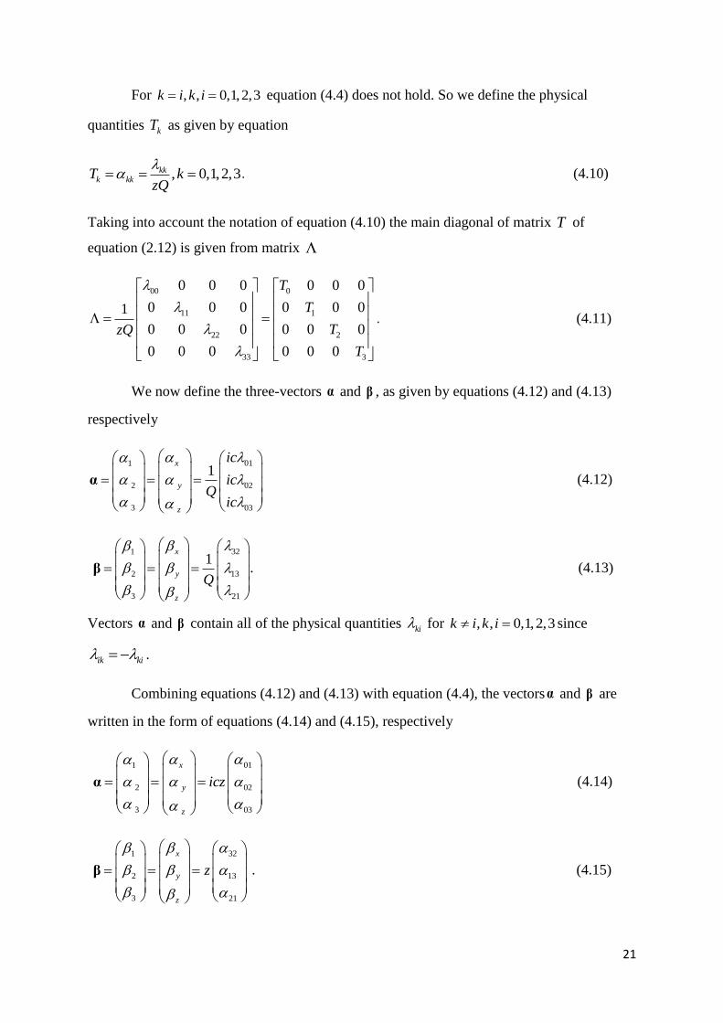
For , , 0,1,2,3k i k i equation (4.4) does not hold. So we define the physical

quantities kT as given by equation

, 0,1,2,3kkk kkT k

zQ

. (4.10)

Taking into account the notation of equation (4.10) the main diagonal of matrix T of

equation (2.12) is given from matrix

00 0

11 1

22 2

33 3

0 0 0 0 0 0

0 0 0 0 0 01

0 0 0 0 0 0

0 0 0 0 0 0

T

T

TzQ

T

. (4.11)

We now define the three-vectors α and β , as given by equations (4.12) and (4.13)

respectively

011

2 02

3 03

1x

y

z

ic

icQ

ic

α (4.12)

321

2 13

3 21

1x

y

z

Q

β . (4.13)

Vectors α and β contain all of the physical quantities ki for , , 0,1,2,3k i k i since

ik ki .

Combining equations (4.12) and (4.13) with equation (4.4), the vectorsα and β are

written in the form of equations (4.14) and (4.15), respectively

011

2 02

3 03

x

y

z

icz

α (4.14)

321

2 13

3 21

x

y

z

z

β . (4.15)

22

We write equation (2.10) in the form

, k,i 0,1,2,3.ik i ki

k

J bP J

x

(4.16)

The rate of change of the momentum of the material particle equals the sum of the two terms

in the right part of equation (4.16). For 0k , and since 0x ict , equation (83) gives the rate

of change of the particle momentum with respect to time ,t i.e. the physical quantity we call

“force”. By using the concept of force, as defined by Newton, we also have to use the concept

of velocity. For this reason we symbolize u the velocity of the material particle, as given by

equation

1

2

3

x

y

z

uu

u u

u u

u . (4.17)

Also, we define the 4-vector of the four-vector u , as given by equation

0

1

2

3

.x

y

z

icu

uuu

uu

u u

(4.18)


Theorem 4.2. ΄΄ The rates of change with respect to time 0t x ict of the four-vectors J

and P of the momentum of the generalized particle carrying charge Q are given by

equations

0 0

idJ dQ i i

J zQ u Q cdx Qdx c c

u α

α u β

(4.19)

0 0

idP dQ i i

J zQ u Q cdx Qdx c c

u α

α u β

.΄΄ (4.20)

23

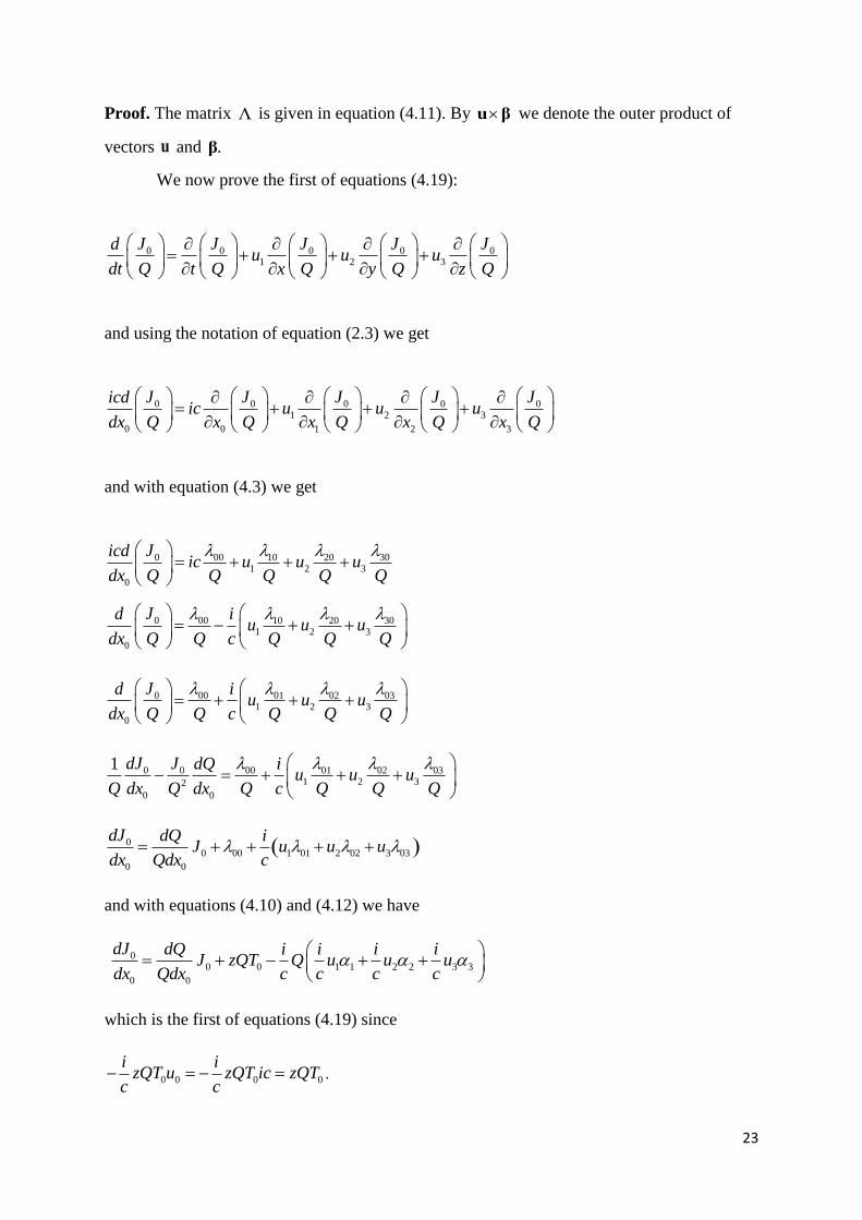
Proof. The matrix is given in equation (4.11). By u β we denote the outer product of

vectors u and .β

We now prove the first of equations (4.19):

0 0 0 0 01 2 3

J J J J Jdu u u

dt Q t Q x Q y Q z Q

and using the notation of equation (2.3) we get

0 0 0 0 01 2 3

0 0 1 2 3

J J J J Jicdic u u u

dx Q x Q x Q x Q x Q


0 00 10 20 301 2 3

0

Jicdic u u u

dx Q Q Q Q Q

0 00 10 20 301 2 3

0

Jd iu u u

dx Q Q c Q Q Q

0 00 01 02 031 2 3

0

Jd iu u u

dx Q Q c Q Q Q

0 0 00 01 02 031 2 32

0 0

1 dJ J dQ iu u u

Q dx Q dx Q c Q Q Q

00 00 1 01 2 02 3 03

0 0

dJ dQ iJ u u u

dx Qdx c

and with equations (4.10) and (4.12) we have

00 0 1 1 2 2 3 3

0 0

dJ dQ i i i iJ zQT Q u u u

dx Qdx c c c c

which is the first of equations (4.19) since

0 0 0 0

i izQT u zQT ic zQT

c c .

24

We prove the second of equations (4.19) and we can similarly prove the third and the

fourth:

1 2 3x x x x xJ J J J Jd

u u udt Q t Q x Q y Q z Q

and using the notation of equations (2.3) and (2.4) we obtain

1 1 1 1 11 2 3

0 0 1 2 3

J J J J Jicd icu u u

dx Q x Q x Q x Q x Q


01 311 11 211 2 3

0

Jicdic u u u

dx Q Q Q Q Q

01 3 131 1 11 2 21

0

iuJ iu iud

dx Q c Q Q c Q c Q

01 3 131 1 1 11 2 21

2

0 0

1 iudJ J iu iudQ

Q dx Q dx c Q Q c Q c Q

31 1 21 11 01 21 13

0 0

iudJ iu iudQJ

dx Qdx c c c

and with equations (4.10), (4.12) and (4.13), we obtain

11 1 1 2 3 3 2

0 0

dJ dQ i i iJ zQT Q Q u u

dx Qdx c c c

which is the second of equations (4.19). Equation (4.20) results from the combination of

equations (4.19) and (3.5).

Using the symbol J for the momentum vector of the material particle

1

2

3

x

y

z

JJ

J J

J J

J

and taking into account equations (2.3) and (2.4) and (4.11) the set of equations (4.19) can be

written in the form

25

2

0

1 1

2 2

3 3

dW dQW zQc T Q

dt Qdt

T ud dQ

zQ T u Qdt Qdt

T u

u α

JJ α u β

. (4.21)

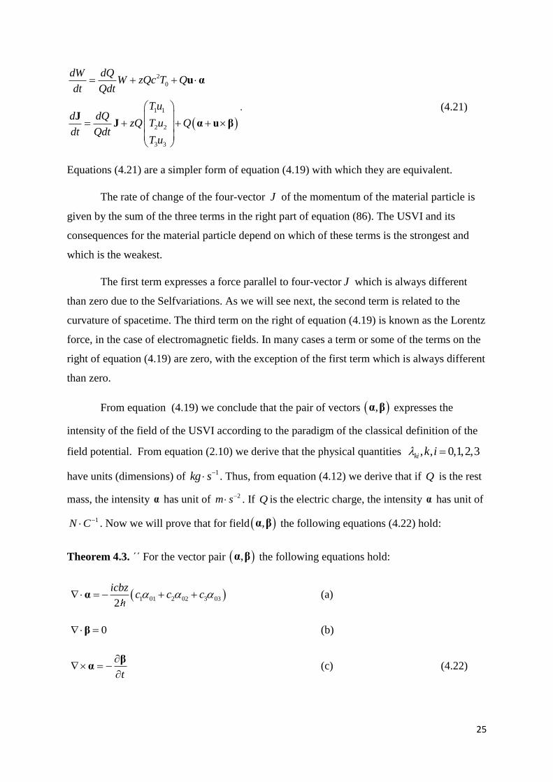
Equations (4.21) are a simpler form of equation (4.19) with which they are equivalent.

The rate of change of the four-vector J of the momentum of the material particle is

given by the sum of the three terms in the right part of equation (86). The USVI and its

consequences for the material particle depend on which of these terms is the strongest and

which is the weakest.

The first term expresses a force parallel to four-vector J which is always different

than zero due to the Selfvariations. As we will see next, the second term is related to the

curvature of spacetime. The third term on the right of equation (4.19) is known as the Lorentz

force, in the case of electromagnetic fields. In many cases a term or some of the terms on the

right of equation (4.19) are zero, with the exception of the first term which is always different

than zero.

From equation (4.19) we conclude that the pair of vectors ,α β expresses the

intensity of the field of the USVI according to the paradigm of the classical definition of the

field potential. From equation (2.10) we derive that the physical quantities , , 0,1,2,3ki k i

have units (dimensions) of 1kg s . Thus, from equation (4.12) we derive that if Q is the rest

mass, the intensity α has unit of 2m s . If Q is the electric charge, the intensity α has unit of

1N C . Now we will prove that for field ,α β the following equations (4.22) hold:

Theorem 4.3. ΄΄ For the vector pair ,α β the following equations hold:

1 01 2 02 3 032

icbzc c c α (a)

0 β (b)

t

βα (c) (4.22)

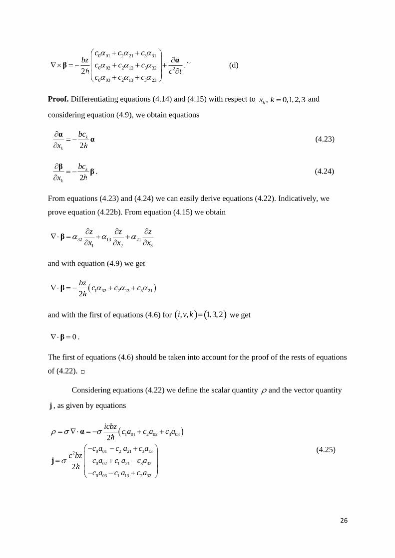
26

0 01 2 21 3 31

0 02 2 12 3 32 2

0 03 2 13 3 23

2

c c cbz

c c cc t

c c c

αβ .΄΄ (d)

Proof. Differentiating equations (4.14) and (4.15) with respect to , 0,1,2,3kx k and

considering equation (4.9), we obtain equations

2

k

k

bc

x

αα (4.23)

2

k

k

bc

x

ββ . (4.24)

From equations (4.23) and (4.24) we can easily derive equations (4.22). Indicatively, we

prove equation (4.22b). From equation (4.15) we obtain

32 13 21

1 2 3

z z z

x x x

β


1 32 2 13 3 212

bzc c c β

and with the first of equations (4.6) for , , 1,3,2i v k we get

0 β .

The first of equations (4.6) should be taken into account for the proof of the rests of equations

of (4.22).

Considering equations (4.22) we define the scalar quantity and the vector quantity

j , as given by equations

1 01 2 02 3 03

0 01 2 21 3 132

0 02 1 21 3 32

0 03 1 13 2 32

2

2

icbzc a c a c a

c a c a c ac bz

c a c a c a

c a c a c a

α

j

(4.25)

27

where 0 is a constant. We now prove that for the physical quantities and j the

following continuity equation holds:

0t

j . (4.26)

Proof. : From the first of equations (4.25) we obtain

t t

t t

α

α

α

and with the second of equations (4.25) and equation (4.22d) we get

2ct

t

β j

j

which is equation (4.26).

According to equation (4.26), the physical quantity is the density of a conserved

physical quantity q with current density j . The conserved physical quantity q is related to

field ,α β through equations (4.22).We will revert to the issue of sustainable physical

quantities in the next chapters.

The density and the current density j have a rigidly defined internal structure as

derived from equations (4.25). We now consider the four-vector of the current density j of

the conserved physical quantity q , as given by equation

0

1

2

3

x

y

z

i cj

jjj

jj

j j

(4.27)

and the 4 4 matrix M

28

01 02 03

01 21 13

02 21 32

03 13 32

0

0

0

0

M

. (4.28)

Using matrix M equations (4.25) can be written in the form of equation

2

2

c bzj MC

. (4.29)

From equations (4.22b,c) we conclude that the potential is always defined in the

,α β - field of the USVI. That is, the scalar potential

0 1 2 3, , , , , ,V V t x y z V x x x x

and the vector potential A

1

0 1 2 3 2

3

, , , , , ,

x

y

z

AA

t x y z x x x x A A

A A

A A A

are defined through the equations

0

icV V

t x

β Α

Α Αα

.

We can introduce in the above equations the gauge function .f That is, we can add to

the scalar potential V the term

0

f ic f

t x

and to the vector potential A the term

f

for an arbitrary function f

0 1 2 3, , , , , ,f f t x y z f x x x x

29

without changing the intensity ,α β of the field. The proof of the above equations is known

and trivial and we will not repeat it here. For the field potential of the USVI the following

theorem holds:

Theorem 4.4.

΄΄1. In the ,α β -field of USVI the pair of scalar-vector potentials ,V A is always defined

through equations

0

0

icV ic A

t x

β Α

Α Αα

. (4.30)

2. The four-vector A of the potential

0

1

2

3

x

y

z

iVA

cA

AAA

AA

A

(4.31)

is given by equation

2, for

, for

ki k

k i

i

k

i

fz i k

b c xA

fi k

x

(4.32)

where 0, 0,1,2,3 , 0,1,2,3kc k i and kf is the gauge function.

3. For 0, , , 0,1,2,3k ic c k i k i equation (4.33) holds

2

2

4, 0, , , 0,1,2,3ki

k i k i

k i

zf f c c k i k i

b c c

. ΄΄ (4.33)

Proof. Equations (4.30) are equivalent to equations (4.22b, c) as we have already mentioned.

The proof of equation (4.32) can be performed through the first of equations (4.6). The

mathematical calculations do not contribute anything useful to our study, thus we omit them.

You can verify that the potential of equation (4.32) gives equations (4.14) and (4.15) through

equations (4.30) taking also into account the first of equations (4.6). □

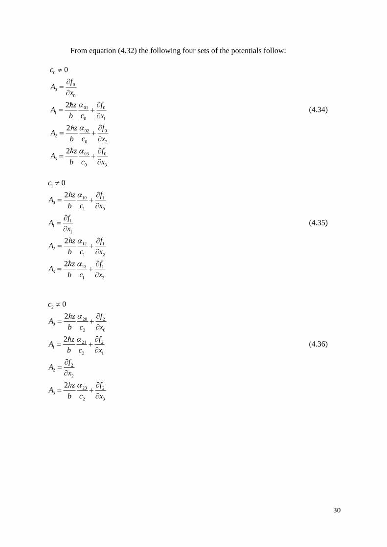
30

From equation (4.32) the following four sets of the potentials follow:

0

00

0

01 01

0 1

02 02

0 2

03 03

0 3

0

2

2

2

c

fA

x

fzA

b c x

fzA

b c x

fzA

b c x

(4.34)

1

10 10

1 0

11

1

12 12

1 2

13 13

1 3

0

2

2

2

c

fzA

b c x

fA

x

fzA

b c x

fzA

b c x

(4.35)

2

20 20

2 0

21 21

2 1

22

2

23 23

2 3

0

2

2

2

c

fzA

b c x

fzA

b c x

fA

x

fzA

b c x

(4.36)

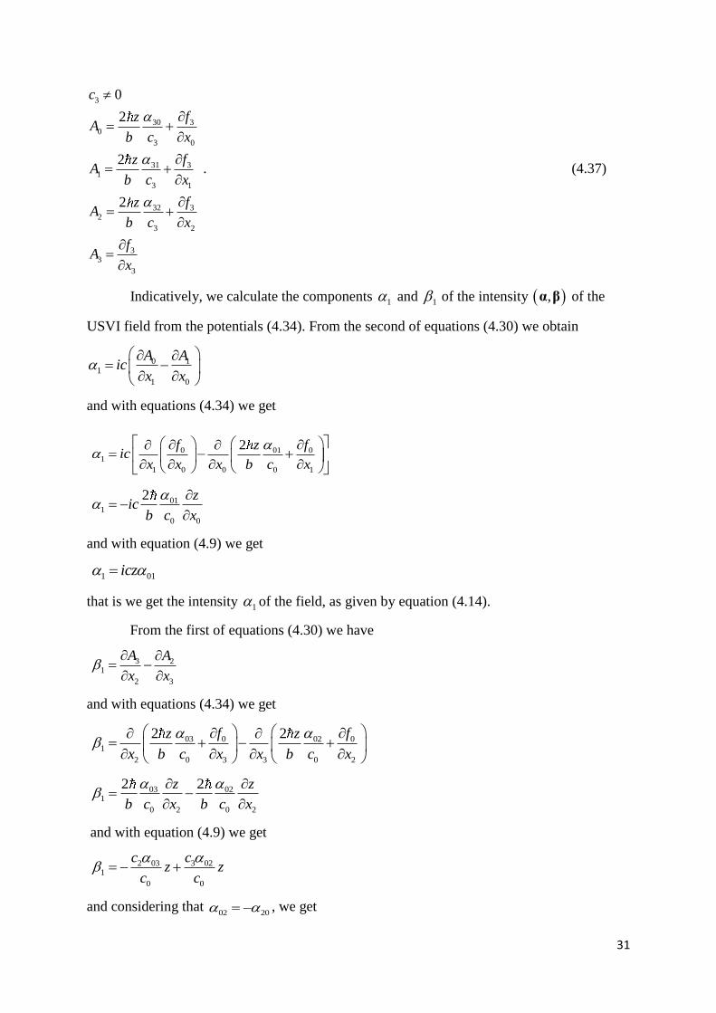
31

3

30 30

3 0

31 31

3 1

32 32

3 2

33

3

0

2

2

2

c

fzA

b c x

fzA

b c x

fzA

b c x

fA

x

. (4.37)

Indicatively, we calculate the components 1 and 1 of the intensity ,α β of the

USVI field from the potentials (4.34). From the second of equations (4.30) we obtain

0 11

1 0

A Aic

x x

and with equations (4.34) we get

0 01 01

1 0 0 0 1

2f fzic

x x x b c x

011

0 0

2 zic

b c x


1 01icz

that is we get the intensity 1 of the field, as given by equation (4.14).

From the first of equations (4.30) we have

3 21

2 3

A A

x x


03 0 02 01

2 0 3 3 0 2

2 2f fz z

x b c x x b c x

03 021

0 2 0 2

2 2z z

b c x b c x


2 03 3 021

0 0

c cz z

c c

and considering that 02 20 , we get

32

1 2 03 3 20

0

zc c

c . (4.38)

From the first of equations (4.6) for , , 2,0,3i v k we obtain

2 03 3 20 0 32

2 03 3 20 0 32

0c a c a c a

c a c a c a

and substituting into equation (4.38), we see that

1 32z

that is, we get the intensity 1 of the field, as given by equation (4.15).

The gauge functions ,k 0,1,2,3kf in equations (4.34)-(4.37) are not independent of

each other. For 0kc and 0ic for , , 0,1,2,3k i k i equation (4.39) holds

2

2

4, 0, , , 0,1,2,3ki

k i k i

k i

zf f c c k i k i

b c c

. (4.39)

The proof of equation (4.39) is through the first of equations (4.6). The proof is

lengthy and we omit it. Indicatively, we will prove the third of equations (4.34) from the third

of equations (4.35) for 1k and 0i in equation (4.39).

For 0 0c and

1 0c both equations (4.34) and equations (4.35) hold. From equation

(4.39) for 1k and 0i we get equation

2

101 0 2

1 0

4 zf f

b c c

. (4.40)

From the third of equations (4.35) and equation (4.40) we get

2

10122 0 2

1 2 0 1

2

0 10122 2

1 2 0 1 2

2 4

2 4

z zA f

b c x b c c

fz zA

b c x b c c x


0 2 10122

1 2 0 1

2 2f cz zA

b c x b c c

02 0 12 2 10

0 1 2

2 fzA c c

bc c x

and since 10 01 , we get equation

02 0 12 2 01

0 1 2

2 fzA c c

bc c x

. (4.41)

33

From the first of equations (4.6) for , , 0,1,2i v k we obtain

0 12 2 01 1 20

0 12 2 01 1 20

0 12 2 01 1 02

0c a c a c a

c a c a c a

c a c a c a

and substituting into equation (4.41) we obtain equation

02 02

0 2

2 fzA

b c x

. (4.42)

Equation (4.42) is the third of equations (4.34).

According to equation (4.39), if 0kc for more than one of the constants

, 0,1,2,3kc k , the sets of equations of potential resulting from equation (4.32) have in the

end a gauge function. In the application we presented assuming 0 0c and

1 0c for a

specific gauge function 0f in equations (4.34), the gauge function 1f in equations (4.35) is

given by equation (4.40).

We conclude the investigation of the potential of the field ,α β of USVI by proving

the following corollary:

Corollary 4.1. ΄΄In the external symmetry, the 4-vector C of the total energy content of the

generalized particle cannot vanish:

0

1

2

3

0

0

0

0

c

cC

c

c

.΄΄ (4.43)

Proof. Indeed, for 0C we obtain J P from equation (3.5). Therefore, the four-vectors

J and P are parallel. According to equivalence (3.7) the parallelism of the four-vectors J

and P is equivalent to the internal symmetry. Therefore, in the external symmetry it is 0C .

A direct consequence of these findings is that the potential of the field ,α β of USVI

is always defined, as given from equation (4.43). This conclusion is derived from the fact that

at least one of the constants , 0,1,2,3kc k is always different than zero.

34

5. THE CONSERVED PHYSICAL QUANTITIES OF THE GENERALIZED

PARTICLE AND THE WAVE EQUATION OF THE TSV

5.1. Introduction

The TSV predicts a wave equation whose special case are the Maxwell equations, the

Schrödinger equation and other relevant equations The wave equation of the TSV is

related to the conserved physical quantities. We determine a mathematical expression for the

total of the conservable physical quantities, and we calculate the current density 4-vector j .

The density and the current density j of the conserved physical quantities have a

strictly determined structure which relates with the quantum behavior of matter. The physical

quantities and j are related with an entirely different way than given by the equation

j u used by the theories of the previous century.

5.2. The conserved physical quantities of the generalized particle and the wave equation

of the TSV

The generalized particle has a set of conserved physical quantities q which we

determine in this chapter. At first, we generalize the notion of the field, as it is derived from

the equations of theTSV. We prove the following theorem:

Theorem 5.1.

΄΄1. For the field ,ξ ω of the pair of vectors

01

02

03

a

ic a

a

ξ (5.1)

32

13

21

a

a

a

ω (5.2)

where 0 1 2 3, , ,x x x x is a function satisfying equation

35

k k

k

bJ P

x

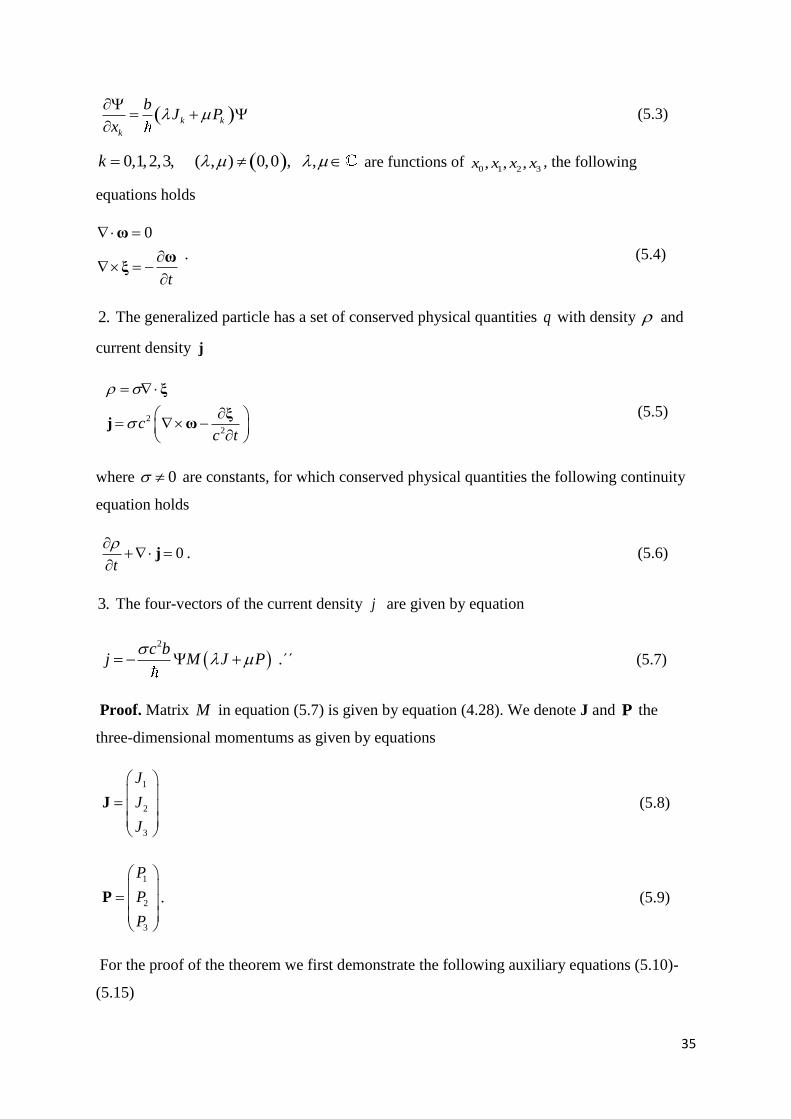
(5.3)

0,1,2,3, ( , ) 0,0 , ,k are functions of 0 1 2 3, , ,x x x x , the following

equations holds

0

t

ω

ωξ

. (5.4)

2. The generalized particle has a set of conserved physical quantities q with density and

current density j

2

2c

c t

ξ

ξj ω

(5.5)

where 0 are constants, for which conserved physical quantities the following continuity

equation holds

0t

j . (5.6)

3. The four-vectors of the current density j are given by equation

2c b

j M J P

.΄΄ (5.7)

Proof. Matrix M in equation (5.7) is given by equation (4.28). We denote J and P the

three-dimensional momentums as given by equations

1

2

3

J

J

J

J (5.8)

1

2

3

P

P

P

P . (5.9)

For the proof of the theorem we first demonstrate the following auxiliary equations (5.10)-

(5.15)

36

32

13

21

0

a

a

a

J (5.10)

32

13

21

0

a

a

a

P (5.11)

01 32

02 0 13

03 21

a a

a J a

a a

J (5.12)

01 32

02 0 13

03 21

a a

a P a

a a

P (5.13)

32 2 21 3 13

13 3 32 1 21

21 1 13 2 32

a J a J a

a J a J a

a J a J a

J (5.14)

32 2 21 3 13

13 3 32 1 21

21 1 13 2 32

a P a P a

a P a Pa

a Pa P a

P . (5.15)

In order to prove equation (5.10) we get

32

13 1 32 2 13 3 21

21

a

a J a J a J a

a

J

and with the second of equations (4.6) for ( , , ) (1,3,2)i v k , we have

32

13

21

0

a

a

a

J

Similarly, from the third of equations (4.6) we obtain equation (5.11). We now get

37

01 2 03 3 02 2 03 3 20

02 3 01 1 03 3 01 1 30

03 1 02 2 01 1 02 2 10

a J a J a J a J a

a J a J a J a J a

a J a J a J a J a

J

and with the second of equations (4.6) we obtain

01 0 32

02 0 13

03 0 21

a J a

a J a

a J a

J

which is equation (5.12). Similarly, by considering the third of equations (4.6) we derive

equation (5.13). Equations (5.14) and (5.15) are derived by taking into account equations

(5.8) and (5.9).

Equations (5.4) are proven with the use of equations (5.10)-(5.15). We prove the first as an

example. From equation (5.2) we obtain

32

13

21

a

a

a

ω


32 32

13 13

21 21

a ab b

a a

a a

ω J P

and with equations (5.10) and (5.11) we obtain

0 ω .

From equations (5.4) and (5.5), the continuity equation (5.6) results. The proof is similar to

the one for equation (4.26). The proof of equation (5.7) is done with the use of equations

(5.10)-(5.15), and equation (4.28).

Field ,α β presented in the previous chapter is a special case of the field ,ξ ω for

1

2 . For these values of the parameteres , we obtain from equations (5.3)

38

1 1

2 2

2

k k

k

k k

k

bJ P

x

bJ P

x


2

k

k

bc

x

and finally we obtain

0 0 1 1 2 2 3 3exp2

bz c x c x c x c x

and from equations (5.1),(5.2) and (4.14),(4.15) we obtain =ξ α and ω β .

From equation (2.10) it emerges that the dimensions of the physical quantities

, , 0,1,2,3ki k i are

1, , 0,1,2,3ki kgs k i .

Thus, from equations (4.12), (4.13) and (4.14), (4.15) we obtain the dimensions of the

physical quantities , , 0,1,2,3kiQ k i . Furthermore, from equation (4.11) we obtain the

dimensions of the physical quantities , 0,1,2,3.kT k Thus, we get the following relationships

1

1

, , , 0,1,2,3,

, 0,1,2,3.

ki

k

Q kgs k i k i

QT kgs k

(5.16)

Using the first of equations (5.16) we can determine the units of measurement of the

,ξ ω -field for every selfvariating charge Q . When Q is the electric charge, we can verify

that the field units are 1,TV m . When Q is the rest mass, the field units are 2 1m s s , .

The dimensions of the field depend solely on the units of measurement of the selfvariating

charge Q .

From equation (5.7) and taking into account that , we can define the

dimensions of the physical quantities q through the first of equations (5.16). When Q is the

electric charge, and for 0 , where 0 is the electric permittivity of the vacuum, q is a

39

conserved physical quantity of electric charge. For 0

e

, where e the constant value we

measure in the lab for the electric charge of the electron, q is a conserved physical quantity

of angular momentum. For 0

e

, q is a dimensionless conserved physical quantity, that

q . When Q is the rest mass, and for 1

4 G

, where G is the gravitational constant, q

is a conserved physical quantity of mass. Theorem 5.1 reveals the conserved physical

quantities of the generalized particle.

One of the most important corollaries of the theorem 5.1 is the prediction that the

generalized particle has wave-like behavior. We prove the following corollary:

Corollary 5.1. ΄΄For function the following equation holds

22 2

2

0

22 2

2 2

i kki

k i

i kki

k i

j jc

x x x

j jc

c t x x

(5.17)

, , 0,1,2,3k i k i .΄΄

Proof. To prove the corollary, considering that 0x ict , we write equations (5.4) and (5.5)

in the form

0

0

2

0

0

1

ij

c

ic

x

i

c c x

ξ

ω

ωξ

ξω j

. (5.18)

We will also use the identity (5.19) which is valid for every vector α

2 α α α . (5.19)

From the third of equations (5.18) we obtain

40

0

0

ic

x

ic

x

ωξ

ξ ω

and using the identity (5.19) we get

2

0

ic

x

ξ ξ ω

and with the first and fourth of equations (5.18) we get

2

2

0 2

0 0

i ij

c x c x

ξ jξ

and we finally get

2

2

02

0 0

ij

x c x

ξ jξ . (5.20)

Working similarly from equation (5.18) we obtain

2

2

2 2

0

1

x c

ωω j . (5.21)

Combining equations (5.20) and (5.21) with equations (5.1) and (5.2), we get

22

2 2

0

, , , 0,1,2,3i kki

k i

j jik i k i

x c x x


Equation (5.17) can be characterized as “the wave equation of the TSV”. The basic

characteristics of equation (5.17) depend on whether the physical quantity

2 2

2 2

2 2 2 2

0

Fx c t

(5.22)

is zero or not.

This conclusion is drawn through the following theorem:

41

Theorem 5.2. ΄΄For the generalized particle the following equivalences hold

2

2

2 20

c t

(5.23)

if and only if for each , , 0,1,2,3k i k i it is

i k

k i

j j

x x

(5.24)

if and only if

22

2 2

22

2 2

0

0

c t

c t

ξξ

ωω

.΄΄ (5.25)

Proof. In the external symmetry there exists at least one pair of indices

( , ), , , 0,1,2,3k i k i k i , for which 0ki . Therefore, when equation (5.24) holds, then

equation (5.23) follows from equation (5.17), and vice versa. Thus, equations (5.23) and

(5.24) are equivalent. When equation (5.24) holds, then the right hand sides of equations

(5.24) and (5.25) vanish, that is, equations (5.25) hold. The converse also holds, thus

equations (5.24) and (5.25) are equivalent. Therefore, equations (5.23), (5.24), and (5.25) are

equivalent. □

In case that 0F , that is in case that equivalences (5.23), (5.24) and (5.25) hold, we

shall refer to the state of the generalized particle as the “generalized photon”. According to

equations (5.25), for the generalized photon the ,ξ ω -field is propagating with velocity c in

the form of a wave. For the generalized photon, the following corollary holds:

Corollary 5.2: ΄΄ For the generalized photon, the four-vector j of the current density of the

conserved physical quantities q , varies according to the equations

2

2

2 20, 0,1,2,3k

k

jj k

c t

.΄΄ (5.26)

Proof. We prove equation (5.26) for 0k , and we can similarly prove it for 1,2,3k .

Considering equation (4.27), we write equation (5.6) in the form

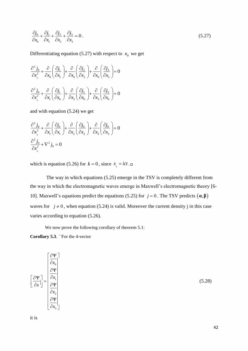
42

0 31 2

0 1 2 3

0j jj j

x x x x

. (5.27)

Differentiating equation (5.27) with respect to 0x we get

0

2

0 31 2

2

0 1 0 2 0 3

0j jj j

x x x x x x x

0

2

0 31 2

2

1 0 2 0 3 0

0j jj j

x x x x x x x


0

0

2

0 0 0 0

2

1 1 2 2 3 3

220

02

0

0

j j j j

x x x x x x x

jj

x

which is equation (5.26) for 0k , since 0

x ict .

The way in which equations (5.25) emerge in the TSV is completely different from

the way in which the electromagnetic waves emerge in Maxwell’s electromagnetic theory [6-

10]. Maxwell’s equations predict the equations (5.25) for 0j . The TSV predicts ,α β

waves for 0j , when equation (5.24) is valid. Moreover the current density j in this case

varies according to equation (5.26).

We now prove the following corollary of theorem 5.1:

Corollary 5.3. ΄΄For the 4-vector

0

1

2

3

x

x

x

x

x

(5.28)

it is

43

2

1M j

x c

(5.29)

where

01 02 03

01 21 13

02 21 32

03 13 32

0

0

0

0

M

and j the 4-vector of the current density of the conserved physical quantities of the

generalized particle.΄΄

Proof. From equation (5.3) and with the notation of equation (5.28) we have

b

J Px

and multiplying from the left with the matrix M we get

b

M M J Px


2

1M j

x c


The equations (5.3), (5.7) and (5.29) give the relation of the wave function with the

physical quantities J , P and j of the generalized particle.

One of the most important conclusions of the theorem 5.1 is that it gives the degrees

of freedom of the equations of the TSV. In equation (5.7) the parameters

, , ( , ) (0,0) can have arbitrary values or can be arbitrary functions of 0 1 2 3, , ,x x x x .

The TSV has two degrees of freedom. Therefore, the investigation of the TSV takes place

through the parameters and of equation (5.7).

If we set , , 1,0,b i or , ,0i

b

in equation (5.7), we get equations

0

0

iJ

x

i

J

. (5.30)

44

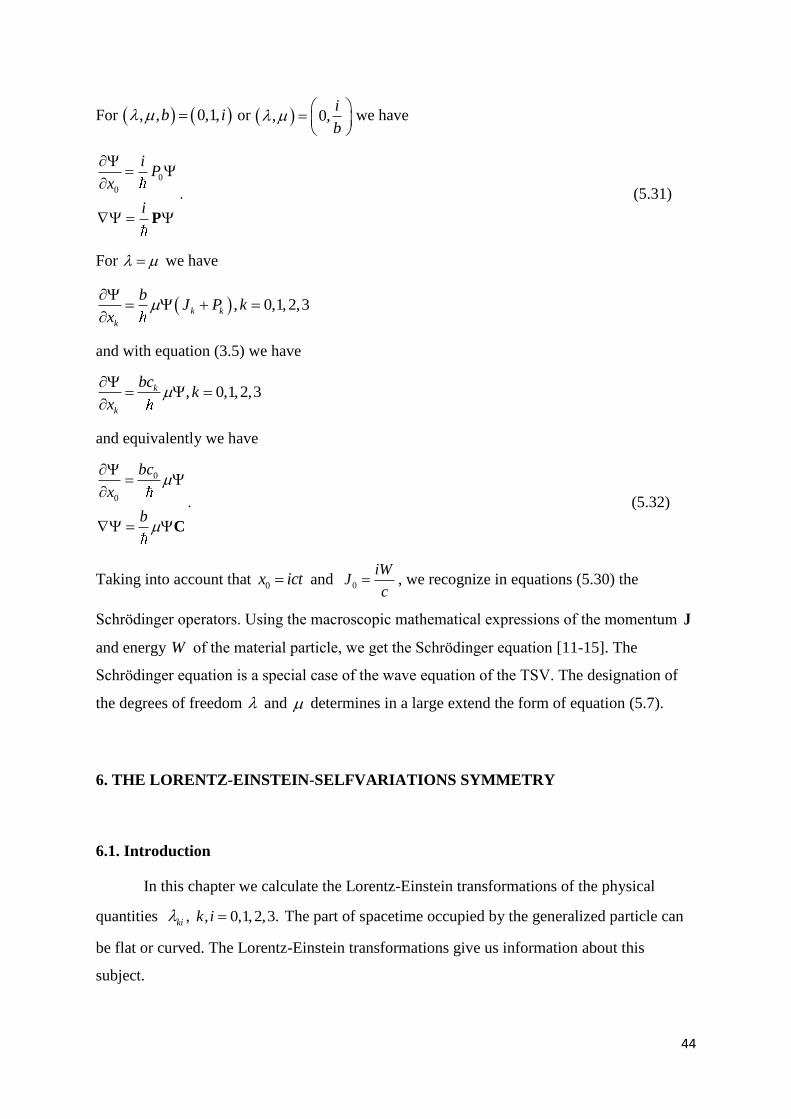
For , , 0,1,b i or , 0,i

b

we have

0

0

i

i

Px

P

. (5.31)

For we have

, 0,1,2,3k k

k

bJ P k

x


, 0,1,2,3k

k

bck

x

and equivalently we have

0

0

bc

x

b

C

. (5.32)

Taking into account that 0x ict and 0

iWJ

c , we recognize in equations (5.30) the

Schrödinger operators. Using the macroscopic mathematical expressions of the momentum J

and energy W of the material particle, we get the Schrödinger equation [11-15]. The

Schrödinger equation is a special case of the wave equation of the TSV. The designation of

the degrees of freedom and determines in a large extend the form of equation (5.7).

6. THE LORENTZ-EINSTEIN-SELFVARIATIONS SYMMETRY

6.1. Introduction

In this chapter we calculate the Lorentz-Einstein transformations of the physical

quantities ki , , 0,1,2,3.k i The part of spacetime occupied by the generalized particle can

be flat or curved. The Lorentz-Einstein transformations give us information about this

subject.

45

The spacetime curvature depends on the elements 00 11 22 33, , , of the main diagonal

of the matrix T of the TSV. We prove that if 0kk for at least one 0,1,2,3k spacetime

is curved. For 00 11 22 33 0 spacetime may be either curved or the flat spacetime of

special relativity.

6.2. The Lorentz-Einstein-Selfvariations Symmetry

We consider an inertial frame of reference , x , y ,zO t moving with velocity

,0,0u with respect to another inertial frame of reference , x, y, zO t , with their origins O

and O coinciding at 0t t . We will calculate the Lorentz-Einsteintransformations for the

physical quantities , , 0,1,2,3ki k i . We begin with transformations (6.1) and (6.2)

2

ut t x

u

x x c t

y y

z z

(6.1)

2

x

x x

y y

z z

W W uJ

uJ J W

c

J J

J J

2

x

x x

y y

z z

E E uP

uP P E

c

P P

P P

(6.2)

where

12 2

21 .

u

c

We then use the notation (2.3), (2.4), (2.5) and obtain the transformations (6.3) and (6.4)

46

0 10

1 01

22

33

ui

x c xx

ui

x c xx

xx

xx

(6.3)

0 0 1

1 1 0

2 2

3 3

uJ J i J

c

uJ J i J

c

J J

J J

0 0 1

1 1 0

2 2

3 3

uP P i P

c

uP P i P

c

P P

P P

. (6.4)

We now derive the transformation of the physical quantity 00 . From equation (2.10)

for 0k i we get for the inertial reference frame , x , y ,zO t

000 0 0

0

J bP J

x

and with transformations (6.3) and (6.4) we obtain

2 2

00 0 1 0 1 0 1

0 1

2 22 0 01 1

00 0 0 0 1 1 0 1 12 2

0 0 1 1

u u b u ui J i J P i P J i J

x c x c c c

J JJ Ju u u b u b u b u bi i P J i P J i PJ PJ

x c x c x c x c c c

and replacing physical quantities

0 01 1

0 0 1 1

, , ,J JJ J

x x x x

from equation (2.10) we get

47

22

00 0 0 00 0 1 01 1 0 10 1 12

2 2

11 0 0 0 1 1 0 1 12 2

(

)

b u b u u b u u bP J i P J i i PJ i PJ

c c c c c

u b u b u b u bP J i P J i PJ PJ

c c c c

and we finally obtain equation

22

00 00 01 10 112

u u ui ic c c

.

Following the same procedure for , i 0,1,2,3k we obtain the following 16 equations

(27) for the Lorentz-Einstein transformations of the physical quantities ki :

22

00 00 01 10 112

22

01 01 00 11 102

02 02 12

03 03 13

u u ui ic c c

u u ui ic c c

uic

uic

22

10 10 11 00 012

22

11 11 10 01 002

12 12 02

13 13 03

u u ui ic c c

u u ui ic c c

uic

uic

(6.5)

48

20 20 21

21 21 20

22 22

23 23

uic

uic

.

The first two of equations (6.5) is self-consistent when equation

00 11 . (6.6)

Then by the second of equations (6.5) we obtain

01 01 .

According to equivalence (3.14) these transformations relate to the external symmetry, in

which it holds that ik ki for , , 0,1,2,3i k i k . Thus, we obtain the following

transformations for the physical quantities , , 0,1,2,3ki k i

00 00

11 11

22 22

33 33

01 01

02 02 21

03 03 13

32 32

13 13 03

21 21 02

uic

uic

uic

uic

. (6.7)

Taking into account equations (4.4), (4.10) and that the physical quantity zQ is invariant

under the Lorentz-Einstein transformations, we obtain the following transformations for the

constants , , , 0,1,2,3ki k i k i and the physical quantities , 0,1,2,3kT k

49

0 0

1 1

2 2

3 3

T T

T T

T T

T T

01 01

02 02 21

03 03 13

32 32

13 13 03

21 21 02

uic

uic

uic

uic

. (6.8)

Equation (6.6) correlates the physical quantities 00 and 11 in the same inertial frame

of reference. Taking into account equation (4.10) we obtain 0 1T T . Thus, when

transformations (6.8) hold, 0 1T T also holds. The reference frame , , ,t x y z moves

with respect to the reference frame , , ,t x y z with constant velocity along the .x -axis. If

we assume that the motion is along the y - or z -axis, the generalization of equation 0 1T T

follows; the Lorentz-Einstein transformations lead to the following equation

0 1 2 3 0T T T T . Thus, we derive the following two corollaries.

Corollary 6.1. ΄΄ When the portion of spacetime occupied by the generalized particle is flat,

it is

0 1 2 3 0T T T T .΄΄ (6.9)

Corollary 6.2.΄΄When

0kT (6.10)

for at least one 0,1,2,3k the portion of spacetime occupied by the generalized particle is

curver and not flat.΄΄

Notice that from the way of proof of corollary 6.1 it follows that the converse is not

true. For external symmetries which have 0 1 2 3 0T T T T , spacetime may be either flat

or curved. In chapter 9 we have shown how to check if spacetime is flat or curved for

external symmetries with 0 1 2 3 0T T T T .

50

In the external symmetry it is 0ki for at least on pair of indices , 0,1,2,3k i .

Thus, in external symmetry it is 0ki only for some pairs of indices , 0,1,2,3k i . The

Lorentz-Einstein transformations reveal that in flat spacetime this cannot be arbitrary. Let’s

assume that it is

02 0

for every inertial frame of reference. Then, we obtain

02 0

and with transformations (6.8) we obtain

02 21 0u

ic

and since it is 02 0 we obtain that it also holds

21 0 .

Working similarly with all of the transformations (6.8) we end up with the following four sets

of equations of external symmetry in the flat spacetime:

0 1 2 3

01 01

02

03

32

13

21

0

0 0

0

0

0

0

0

T T T T

(6.11)

0 1 2 3

01 01

02

03

32 32

13

21

0

0 0

0

0

0 0

0

0

T T T T

(6.12)

51

0 1 2 3

01 01

02 02

03

32 32

13

21 21

0

0 0

0 0

0

0 0

0

0 0

T T T T

(6.13)

0 1 2 3

01 01

02

03 03

32 32

13 13

21

0

0 0

0

0 0

0 0

0 0

0

T T T T

. (6.14)

As we will see the number of external symmetries in four-dimensional spacetime is

59. From these 2 4 16 16 38 cases, 9 are discarded and only 29 are external

symmetries which belong to the set of 59external symmetries. The symmetry that equations

(6.11)-(6.14) express will be referred to as the symmetry of the Lorentz-Einstein-

Selfvarlations. These symmetries hold only in case that the part of spacetime occupied by the

generalized particle is flat.

7. THE FUNDAMENTAL STUDY FOR THE CORPUSCULAR STRUCTURE OF

MATTER IN EXTERNAL SYMMETRY. THE Π-PLANE. THE SV T METHOD

7.1. Introduction

The material particles are in a constant interaction between them (via the USVI)

because of STEM. This interaction has consequences in the internal structure of the

generalized particle, including the distribution of its total energy and momentum between the

material particle and the surrounding spacetime.

The internal structure of the generalized particle is determined by the relations among

the elements of the matrix T . The same holds for the rest mass 0m of the material particle, the

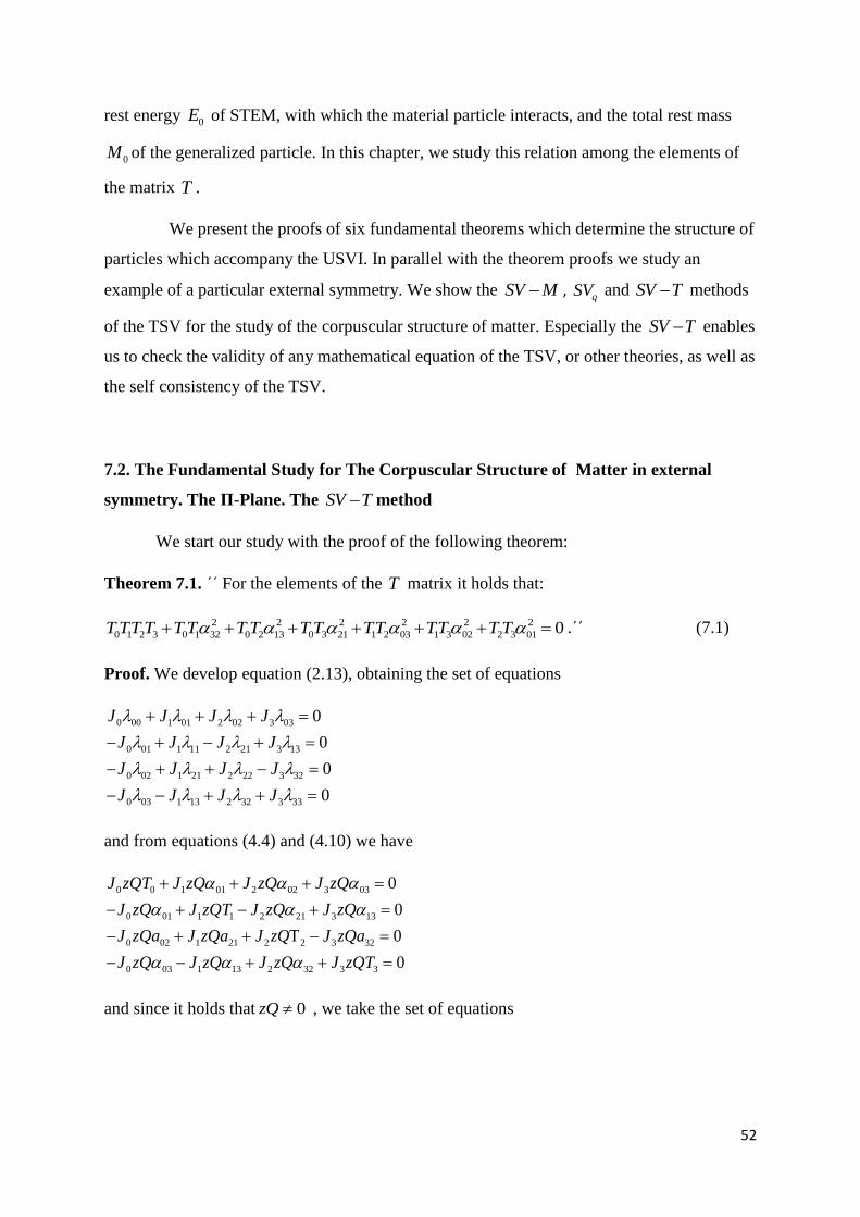
52

rest energy 0E of STEM, with which the material particle interacts, and the total rest mass

0M of the generalized particle. In this chapter, we study this relation among the elements of

the matrix T .

We present the proofs of six fundamental theorems which determine the structure of

particles which accompany the USVI. In parallel with the theorem proofs we study an

example of a particular external symmetry. We show the SV M , qSV and SV T methods

of the TSV for the study of the corpuscular structure of matter. Especially the SV T enables

us to check the validity of any mathematical equation of the TSV, or other theories, as well as

the self consistency of the TSV.

7.2. The Fundamental Study for The Corpuscular Structure of Matter in external

symmetry. The Π-Plane. The SV T method

We start our study with the proof of the following theorem:

Theorem 7.1. ΄΄ For the elements of the T matrix it holds that:

2 2 2 2 2 2

0 1 2 3 0 1 32 0 2 13 0 3 21 1 2 03 1 3 02 2 3 01 0T TT T T T T T T T TT TT T T .΄΄ (7.1)

Proof. We develop equation (2.13), obtaining the set of equations

0 00 1 01 2 02 3 03

0 01 1 11 2 21 3 13

0 02 1 21 2 22 3 32

0 03 1 13 2 32 3 33

0

0

0

0

J J J J

J J J J

J J J J

J J J J

and from equations (4.4) and (4.10) we have

0 0 1 01 2 02 3 03

0 01 1 1 2 21 3 13

0 02 1 21 2 2 3 32

0 03 1 13 2 32 3 3

0

0

0

0

J zQT J zQ J zQ J zQ

J zQ J zQT J zQ J zQ

J zQa J zQa J zQ J zQa

J zQ J zQ J zQ J zQT

and since it holds that 0zQ , we take the set of equations

53

0 0 1 01 2 02 3 03

0 01 1 1 2 21 3 13

0 02 1 21 2 2 3 32

0 03 1 13 2 32 3 3

0

0

0

0

J T J J J

J J T J J

J J J T J

J J J J T

. (7.2)

The set of equations given in (7.2) comprise a 4 4 homogeneous linear system of equations

with unknowns the momenta 0 1 2 3, , ,J J J J . In order for the material particle to exist, the

system of equations (7.2) must obtain non-vanishing solutions. Therefore, its determinant

must vanish. Thus, we obtain equation

2 2 2 2 2 2

0 1 2 3 0 1 32 0 2 13 0 3 21 1 2 03 1 3 02 2 3 01

2

01 32 02 13 03 21( ) 0

T TT T T T T T T T TT TT T T

and with equation (4.8) we arrive at equation (7.1).

We formulated theorem 7.1 for 0J in order for the material particle to exist. If we

formulate the theorem for 0P , then material particle and the STEM trade places in the

equations and the conclusions of the TSV.

We consider the 4 4 N matrix, given as:

32 13 21

32 03 02

13 03 01

21 02 01

0

0

0

0

N

. (7.3)

Using the matrix N , we now write equation (4.6) in the form of

0

0

0

NC

NJ

NP

. (7.4)

We now prove Lemma 7.1:

Lemma 7.1. ΄΄The four-vectors , ,C J P satisfy the set of equations

2

2

2

0

0

0

N C

N J

N P

.΄΄ (7.5)

54

Proof. We multiply the set of equations (7.4) from the left with the matrix N , and equations

(7.5) follow.

Using lemma 7.1 we prove theorem 7.2 :

Theorem 7.2. ΄΄For 0M it holds that:

1. 0MN NM . (7.6)

2. 2 2 2M N I (7.7)

2 2 2 2 2 2 2

01 02 03 32 13 21 . (7.8)

Here, I is the 4 4 identity matrix.

3. For 0 the matrix M has two eigenvalues 1 and 2 , with corresponding

eigenvectors 1 and 2 , given by:

1

2 2 2

01 02 03

01 03 13 02 21

1 2

02 01 21 03 32

03 02 32 01 13

0

1

i

i

(7.9)

2

2 2 2

01 02 03

01 03 13 02 21

2 2

02 01 21 03 32

03 02 32 01 13

0

1

i

i

. (7.10)

4. For 0 the matrix N has the same eigenvalues with the matrix M , and two

corresponding eigenvectors 1n and 2n , given by:

1

2 2 2

32 13 21

32 02 21 03 13

1 2

13 03 32 01 21

21 01 13 02 32

0

1

i

in

(7.11)

55

2

2 2 2

32 13 21

32 02 21 03 13

2 2

13 03 32 01 21

21 01 13 02 32

0

1

i

in

. (7.12)

5. When 2 2 , , , 0,1,2,3ki k i k i is

2 2 2 2 2 2 2

01 02 03 32 13 21 0 (7.13)

2

2

2

0

0

0

M C

M J

M P

. (7.14)

6. For 2 2 , , , 0,1,2,3ki k i k i it con be

2 0 .΄΄

Proof. The matrices M and N are given by equations (4.28) and (7.3). The proof of

equations (7.6), (7.7), (7.9), (7.10), (7.11) and (7.12) can be performed by the appropriate

mathematical calculations and the use of equation (4.8).

We multiply equation (7.7) from the right with the column matrices , ,C J P , and

obtain

2 2 2

2 2 2

2 2 2

M C N C C

M J N J J

M P N P P

and from equations (7.5) we obtain

2 2

2 2

2 2

M C C

M J J

M P P

. (7.15)

According to the set of equations (7.15), and for 0 , 2 2 , , , 0,1,2,3ki k i k i ,

the matrix 2 0M has as eigenvalue 2 0 with corresponding eigenvector 0 . From

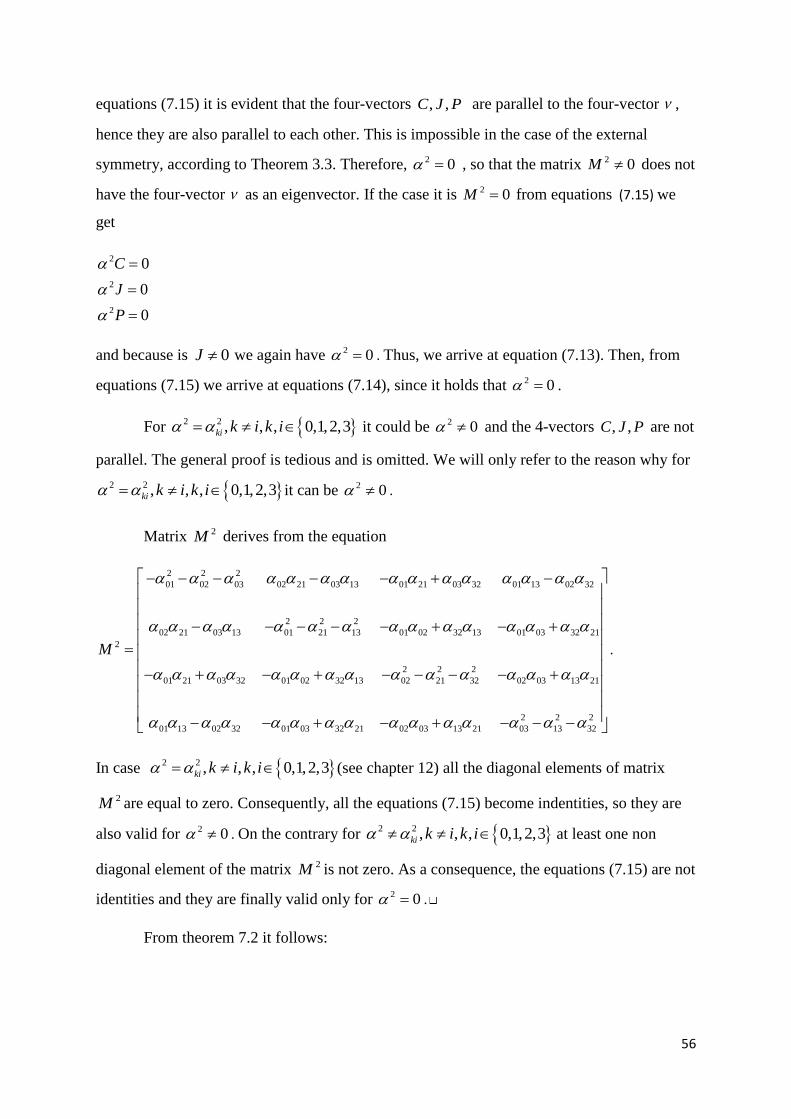
56

equations (7.15) it is evident that the four-vectors , ,C J P are parallel to the four-vector ,

hence they are also parallel to each other. This is impossible in the case of the external

symmetry, according to Theorem 3.3. Therefore, 2 0 , so that the matrix 2 0M does not

have the four-vector as an eigenvector. If the case it is 2 0M from equations (7.15) we

get

2

2

2

0

0

0

C

J

P

and because is 0J we again have 2 0 . Thus, we arrive at equation (7.13). Then, from

equations (7.15) we arrive at equations (7.14), since it holds that 2 0 .

For 2 2 , , , 0,1,2,3ki k i k i it could be 2 0 and the 4-vectors , ,C J P are not

parallel. The general proof is tedious and is omitted. We will only refer to the reason why for

2 2 , , , 0,1,2,3ki k i k i it can be 2 0 .

Matrix 2M derives from the equation

2 2 2

01 02 03 02 21 03 13 01 21 03 32 01 13 02 32

2 2 2

02 21 03 13 01 21 13 01 02 32 13 01 03 32 21

2

2 2 2

01 21 03 32 01 02 32 13 02 21 32 02 03 13 21

01 13 02 32 01 03 32 21

M

2 2 2

02 03 13 21 03 13 32

.

In case 2 2 , , , 0,1,2,3ki k i k i (see chapter 12) all the diagonal elements of matrix

2M are equal to zero. Consequently, all the equations (7.15) become indentities, so they are

also valid for 2 0 . On the contrary for 2 2 , , , 0,1,2,3ki k i k i at least one non

diagonal element of the matrix 2M is not zero. As a consequence, the equations (7.15) are not

identities and they are finally valid only for 2 0 .

From theorem 7.2 it follows:

57

Corollary 7.1. ΄΄For the four-vector j of the conserved physical quantities q it holds that:

1. 0Mj , for 2 2 , , , 0,1,2,3ki k i k i . (7.16)

2. 0Nj .΄΄ (7.17)

Proof. We multiply equation (5.7) by matrix M from the left and obtain

2

2 2c bMj M J M P

and with the second and the third of equations (7.14) we have

0Mj .

We multiply the terms of equation (5.7) from the left with the matrix N , and obtain

2c b

Nj NM J P

and with equation (7.6) we take

0Nj .

In the equations of the TSV there appear sums of squares that vanish, like the ones

appearing in equations (3.6) and (7.13). Writing these equations in a suitable manner, we can

introduce into the equations of the TSV complex numbers. From equation (3.6) , and for

0 0M , we obtain

2 2 2 2

0 31 2

0 0 0 0

1 0c cc c

M c M c M c M c

.

Therefore, the physical quantities

0 31 2

0 0 0 0

, , ,c cc c

M c M c M c M c

belong in general to the set of complex numbers . This transformation of the equations of

the TSV is not necessary. It suffices to remember that within the equations of the TSV there

are sums of squares that vanish. We now prove theorem 7.3, which also intercorrelates the

elements of the matrix T :

58

Theorem 7.3. ΄΄In the external symmetry and for the elements of the matrix T it holds that:

0

, , , , , 0,1,2,3

i kTa

i k k i i k

.΄΄ (7.18)

Proof. We differentiate the second equation of the set of equations (4.6)

0

, , , , , 0,1,2,3

i k k i kiJ J J

i k k i i k

with respect to , 0,1,2,3jx j . Considering equations (2.10) and (4.4), we have

0k j i ji i j k jk ki j j

b b bP J zQ P J zQ P J zQ

0j i k k i ki k ji i jk ki j

bP J J J zQ

and with the second equation of the set of equations (4.6), and taking into account that

0zQ , we obtain

0

, , , , , , 0,1,2,3

k ji i jk ki j

i k k i i k j

. (7.19)

Inserting into equation (7.19) successively , , 0,1,2 , 0,1,3 , 0,2,3 , 1,2,3i k and

0,1,2,3j , we arrive at the set of equations

0 32

0 13

0 21

1 02

1 03

1 32

2 01

2 03

2 13

3 01

3 02

3 21

0

0

0

0

0

0

0

0

0

0

0

0

T

T

T

T

T

T

T

T

T

T

T

T

. (7.20)

The set of equations (7.20) is equivalent to equation (7.18).

59

Theorem 7.3 is one of the most powerful tools for investigating the external

symmetry. This results from corollary 7.2 :

Corollary 7.2. ΄΄For the elements of the matrix T of the external symmetry the following

hold:

1. For every , , , , , 0,1,2,3k i k i k i it holds that

0

0

,

ki

k i

k i

. (7.21)

2.

0 32 13 21

1 02 03 32

2 01 03 13

3 01 02 21

0 0

0 0

0 0

0 0

T

T

T

T

.΄΄ (7.22)

Proof. Corollary 7.2 is an immediate consequence of theorem 7.3.

From theorem 7.3 the following corollary follows, regarding the elements of the main

diagonal of the matrices of the external symmetry:

Corollary 7.3. ΄΄At least one of the elements of the main diagonal of the matrix T is equal

to zero.΄΄

Proof. If 0T for every 0,1,2,3 , from equations (7.20) we obtain 0ki for every

set of indices , , 0,1,2,3k i k i , and from equation (7.1) we have

0 1 2 3 0T TT T .

This cannot hold, since we assumed that 0T for every 0,1,2,3 . Therefore, at least one

element of the main diagonal of the matrix T is equal to zero.

We present a second way for proving this result. In the case of 0T for every

0,1,2,3 , we obtain from equations (7.20) that 0ki , for every , , 0,1,2,3k i k i .

Thus, the matrix T takes the form

60

0

1

2

3

0 0 0

0 0 0

0 0 0

0 0 0

T

TT zQ

T

T

.

From equation (2.13) we take

0 0 1 1 2 2 3 3 0T J T J T J T J

Since we assumed that

0 1 2 3 0T TT T

we obtain

0 1 2 3 0J J J J .

Thus, the material particle does not exist.

The corollary 7.3 follows from the combination of theorems 7.1 and 7.3. We write the

equation (7.1)

2 2 2 2 2 2

0 1 2 3 0 1 32 0 2 13 0 3 21 1 2 03 1 3 02 2 3 01 0T TT T T T T T T T TT TT T T

in the form

0 1 2 3 0 32 1 32 0 13 2 13 0 21 3 21 1 03 2 03 1 02 3 02 2 01 3 01 0T TT T T T T T T T T T T T T T

and continuing with equations (7.20) we get

0 1 2 3 0T TT T

which implies that not all physical quantities 0 1 2 3, , ,T T T T can be nonzero. Notice that theorem

7.1 is a consequence of the relation 0J , which also lies ‘behind’ the proof of corollary 7.3

we presented above.

We consider now the three-dimensional vectors

1 32

2 13

3 21

τ (7.23)

61

1 01

2 02

3 03

n

n

n

n . (7.24)

In the case of the T matrices with τ 0 and n 0 , we define the vector μ 0 from equation

1 02 21 03 13

2 03 32 01 21

3 01 13 02 32

μ . (7.25)

Combining equations (5.1), (5.2) with equations (7.23) and (7.24) we obtain

ic ξ n (7.26)

ω τ . (7.27)

The field ξ is parallel to the vector n and the field ω is parallel to the vector τ . Moreover the

only variable quantity of the field , ξ ω is the function 0 1 2 3, , ,x x x x .

For every vector

1

2

3

α

which is determined by the physical quantities of the TSV, we define the physical quantity

1 1

2 2 22 21 2 3

T α α α . (7.28)

Here, the matrix Tα is the transposed matrix of the column matrix α .

From equations (7.23) and (7.24) we obtain

01 32 02 13 03 21 τ n .

Also, from equation (4.8) we have

0 τ n . (7.29)

Therefore, the vectors τ and n are perpendicular to each other. Considering also equation

(7.25), we see that the triple of the vectors { , ,μ n τ } forms a right-handed vector basis.

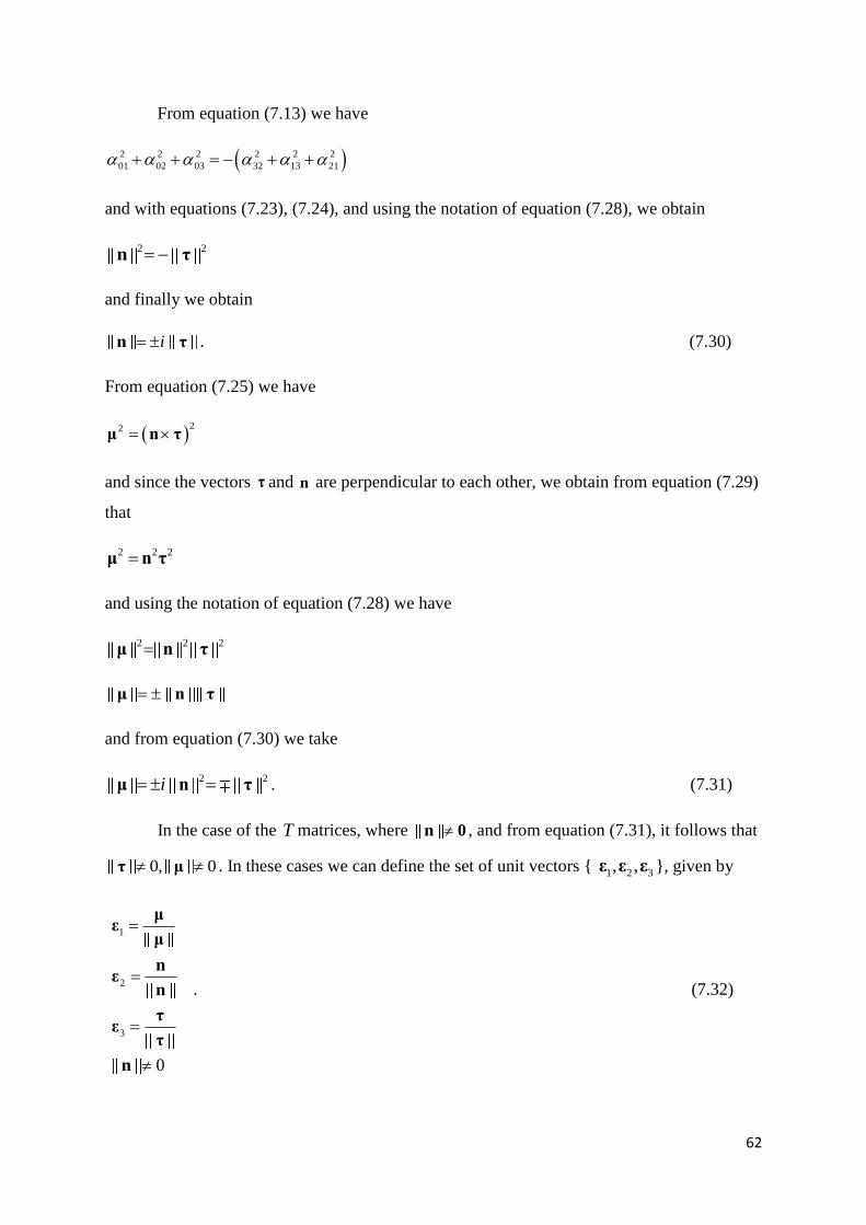
62

From equation (7.13) we have

2 2 2 2 2 2

01 02 03 32 13 21

and with equations (7.23), (7.24), and using the notation of equation (7.28), we obtain

2 2 n τ


i n τ . (7.30)


22 μ n τ

and since the vectors τ and n are perpendicular to each other, we obtain from equation (7.29)

that

2 2 2μ n τ

and using the notation of equation (7.28) we have

2 2 2μ n τ

μ n τ

and from equation (7.30) we take

2 2i μ n τ . (7.31)

In the case of the T matrices, where n 0 , and from equation (7.31), it follows that

0, 0 τ μ . In these cases we can define the set of unit vectors { 1 2 3, ,ε ε ε }, given by

1

2

3

0

με

μ

nε

n

τε

τ

n

. (7.32)

63

The triple of vectors { 1 2 3, ,ε ε ε } forms a right-handed orthonormal vector basis.

In the cases of the T matrices with τ 0 , we define with the plane perpendicular

to the vector τ 0 . In the cases where moreover n 0 , we obtain from equation (7.25) that

μ 0 .In these cases the vectors n and μ are perpendicular to the vector τ , as implied by

equations (7.25) and (7.29). Therefore, the vectors n and μ belong to the plane , and they

also form an orthogonal basis of this plane. We note that the vectors of the TSV, which may

belong to the plane , are given as a linear combination of the vectors n and μ . Therefore,

the condition for τ 0 is not sufficient, in order for the plane to acquire a physical

meaning. Also, we note that because of equation (7.13), the plane , when it is defined, is

not a vector subspace of 3 .

We now prove theorem 7.4:

Theorem 7.4. ΄΄In the case of the T matrices with τ 0 and n 0 and τ n 0 , the

vectors

, , , ,J P C j belong to the same plane .΄΄

Proof. From equations (4.6), for , , 1,3,2i k , we obtain

1 32 2 13 3 21

1 32 2 13 3 21

1 32 2 13 3 21

0

0

0

c c c

J J J

P P P

and from equations (5.8),(5.9) and (7.23) we get

0

0

0

τ C

τ J

τ P

(7.33)

where

C J P (7.34)

as implied by equation (3.5). From equation (7.33) we conclude that the vectors , ,C J P ,

being perpendicular to vector τ , belong to the plane . From equation (5.3) and equations

(5.8) and (5.9) we obtain

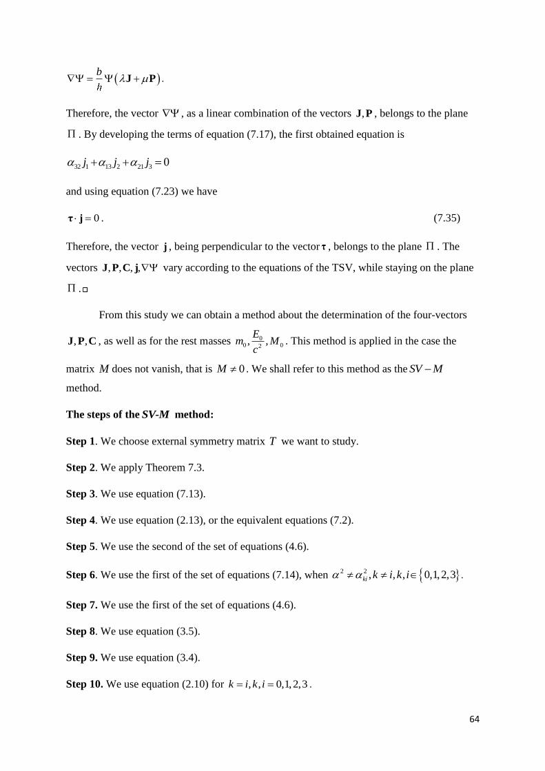
64

b

J P .

Therefore, the vector , as a linear combination of the vectors ,J P , belongs to the plane

. By developing the terms of equation (7.17), the first obtained equation is

32 1 13 2 21 3 0j j j

and using equation (7.23) we have

0 τ j . (7.35)

Therefore, the vector j , being perpendicular to the vector τ , belongs to the plane . The

vectors , , , ,J P C j vary according to the equations of the TSV, while staying on the plane

.

From this study we can obtain a method about the determination of the four-vectors

, ,J P C , as well as for the rest masses 00 02, ,E

m Mc

. This method is applied in the case the

matrix M does not vanish, that is 0M . We shall refer to this method as the SV M

method.

The steps of the SV-M method:

Step 1. We choose external symmetry matrix T we want to study.

Step 2. We apply Theorem 7.3.

Step 3. We use equation (7.13).

Step 4. We use equation (2.13), or the equivalent equations (7.2).

Step 5. We use the second of the set of equations (4.6).

Step 6. We use the first of the set of equations (7.14), when 2 2 , , , 0,1,2,3ki k i k i .

Step 7. We use the first of the set of equations (4.6).



Step 10. We use equation (2.10) for , , 0,1,2,3k i k i .

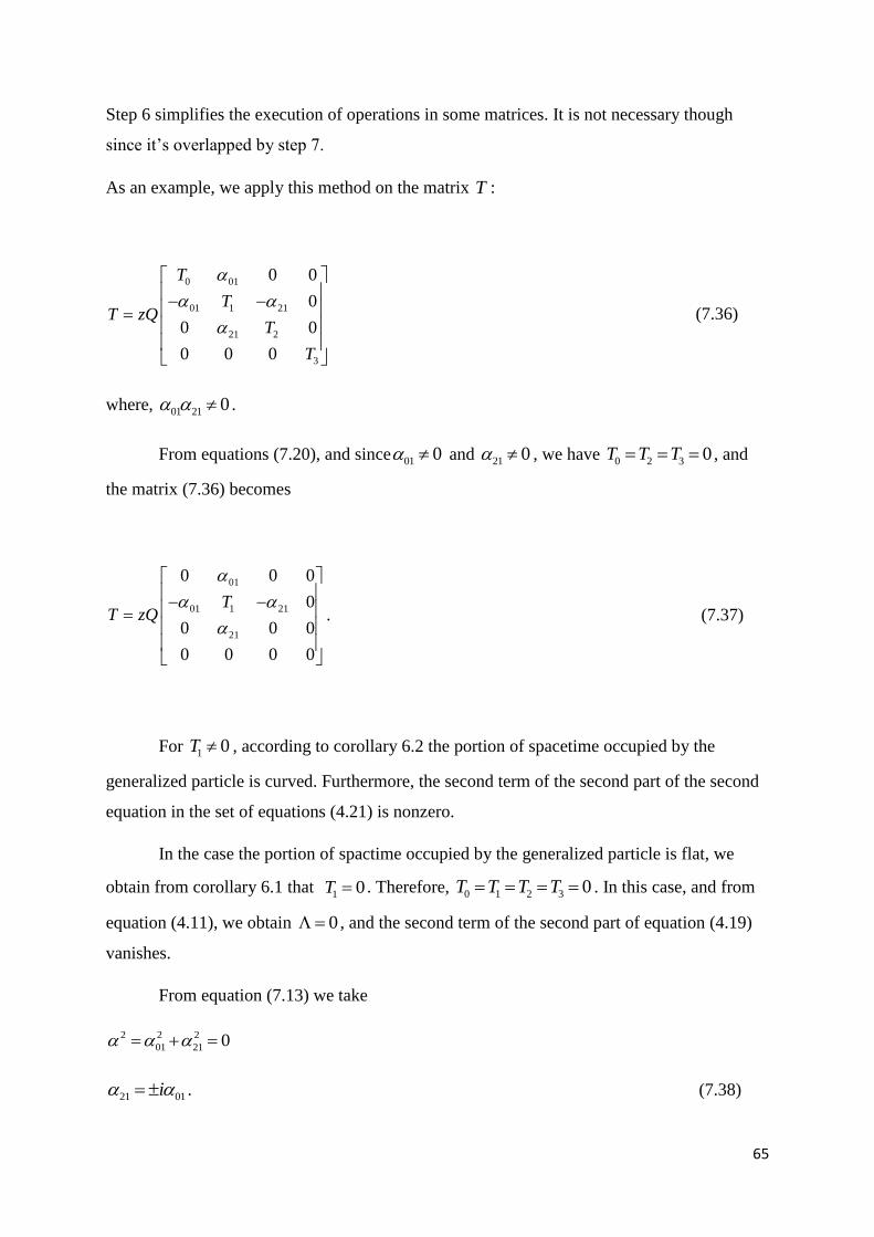
65

Step 6 simplifies the execution of operations in some matrices. It is not necessary though

since it’s overlapped by step 7.

As an example, we apply this method on the matrix T :

0 01

01 1 21

21 2

3

0 0

0

0 0

0 0 0

T

TT zQ

T

T

(7.36)

where, 01 21 0 .

From equations (7.20), and since 01 0 and 21 0 , we have 0 2 3 0T T T , and

the matrix (7.36) becomes

01

01 1 21

21

0 0 0

0

0 0 0

0 0 0 0

TT zQ

. (7.37)

For 1 0T , according to corollary 6.2 the portion of spacetime occupied by the

generalized particle is curved. Furthermore, the second term of the second part of the second

equation in the set of equations (4.21) is nonzero.

In the case the portion of spactime occupied by the generalized particle is flat, we

obtain from corollary 6.1 that 1 0T . Therefore, 0 1 2 3 0T T T T . In this case, and from

equation (4.11), we obtain 0 , and the second term of the second part of equation (4.19)

vanishes.

From equation (7.13) we take

2 2 2

01 21 0

21 01i . (7.38)

66

From equations (7.2) we obtain

1 01

0 01 1 1 2 21

1 21

0

0

0

J

J J T J

J

and since 01 21 0 , we have that

1

012 0

21

0J

J J

. (7.39)

From the second of equations (4.6), for , , 3,0,1i k we have

3 01 1 30 0 13 0J J J

and since

01 30 03 130, 0, 0

we obtain

3 0J . (7.40)

From equations (7.39) and (7.40), and from equation (2.4), we get the four-vector J

0 001

21

11

00 0

1

0 00

i

WJ J J

i c

. (7.41)

For the second equality in equation (7.41) we applied the second equation of equations

(7.38).

From equations (4.29) and (7.37) we have

01

01 21

21

0 0 0

0 0

0 0 0

0 0 0 0

M

(7.42)

67

2

01 01 21

2

2

01 21 21

0 0

0 0 0 0

0 0

0 0 0 0

M

. (7.43)

From the first of equations (7.14) we see that

2 0M C

and with equations (3.5) and (7.43) we obtain

2

01 0 01 21 2

2

01 21 0 21 2

0

0

a c a a c

a a c a c

and taking into account that 01 21 0 , we obtain

012 0

21

c c

. (7.44)

From the first of the equations (4.6), for , , 0,1,2 , 0,1,3 , 0,2,3 , 1,2,3i k we have

0 12 2 01 1 20

0 13 3 01 1 30

0 23 3 02 2 30

1 23 3 12 2 31

0

0

0

0

c c c

c c c

c c c

c c c

and taking into account the zero elements of the matrix T we have

0 21 2 01

3 01

3 12

0

0

0

c c

c

c

and since 01 21 0 we obtain

212 0

01

3 0

c c

c

. (7.45)

The first of equations (7.45) is equation (7.44), because of equation (7.38). From equations

(3.5) and (7.38), (7.45) we obtain the four-vector C

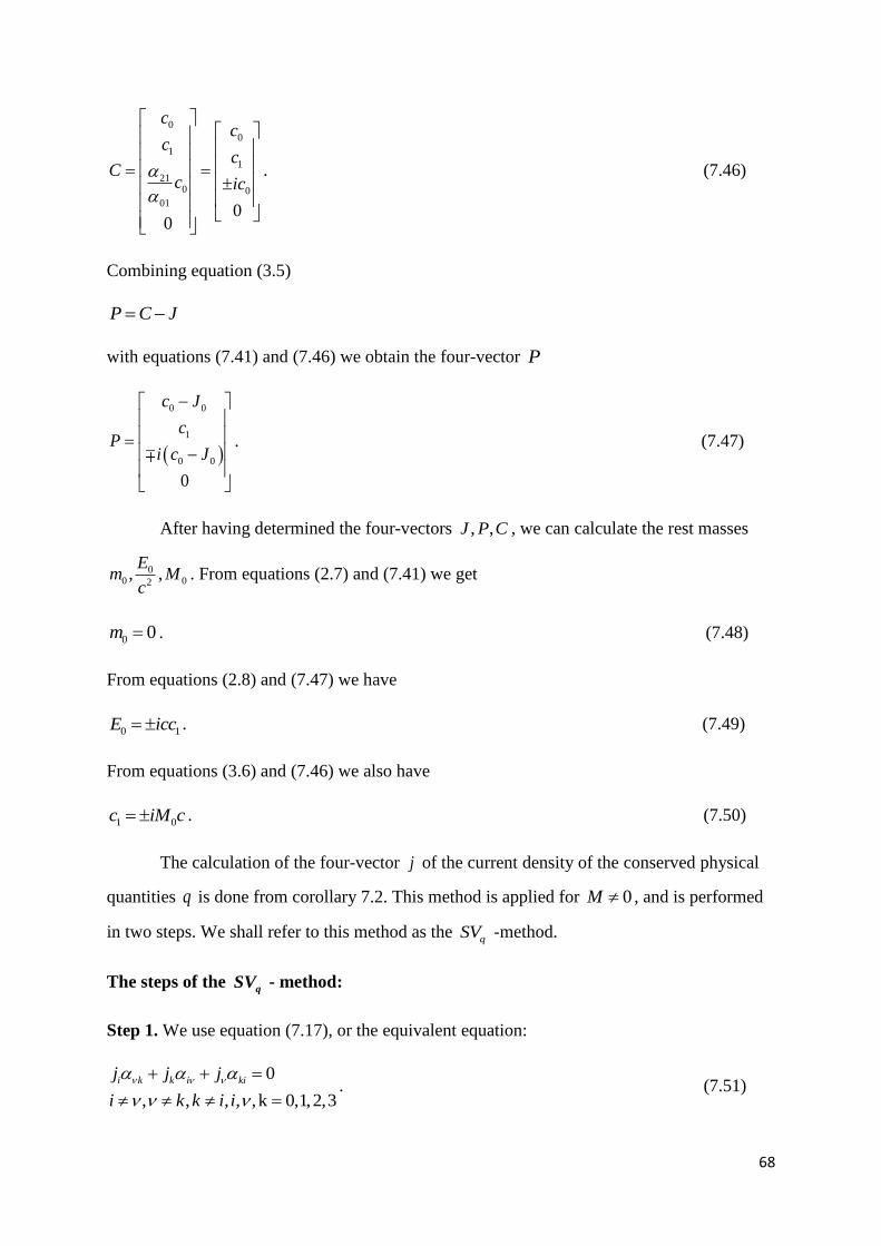
68

0

0

1

1

210 0

010

0

cc

cc

Cc ic

. (7.46)

Combining equation (3.5)

P C J

with equations (7.41) and (7.46) we obtain the four-vector P

0 0

1

0 0

0

c J

cP

i c J

. (7.47)

After having determined the four-vectors , ,J P C , we can calculate the rest masses

00 02, ,E

m Mc

. From equations (2.7) and (7.41) we get

0 0m . (7.48)


0 1E icc . (7.49)

From equations (3.6) and (7.46) we also have

1 0c iM c . (7.50)

The calculation of the four-vector j of the current density of the conserved physical

quantities q is done from corollary 7.2. This method is applied for 0M , and is performed

in two steps. We shall refer to this method as the qSV -method.

The steps of the qSV - method:

Step 1. We use equation (7.17), or the equivalent equation:

0

, , , , ,k 0,1,2,3

i k k i kij j j

i k k i i

. (7.51)

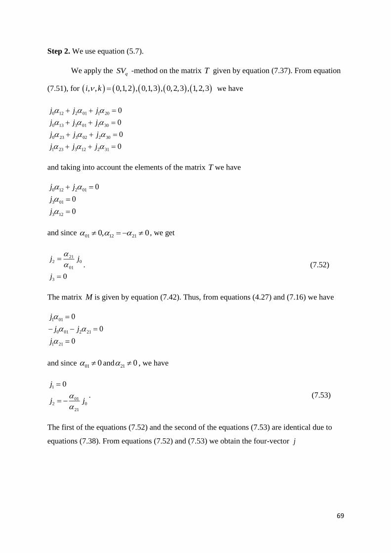
69


We apply the qSV -method on the matrix T given by equation (7.37). From equation

(7.51), for , , 0,1,2 , 0,1,3 , 0,2,3 , 1,2,3i k we have

0 12 2 01 1 20

0 13 3 01 1 30

0 23 3 02 2 30

1 23 3 12 2 31

0

0

0

0

j j j

j j j

j j j

j j j

and taking into account the elements of the matrix T we have

0 12 2 01

3 01

3 12

0

0

0

j j

j

j

and since 01 12 210, 0 , we get

212 0

01

3 0

j j

j

. (7.52)

The matrix M is given by equation (7.42). Thus, from equations (4.27) and (7.16) we have

1 01

0 01 2 21

1 21

0

0

0

j

j j

j

and since 01 0 and 21 0 , we have

1

012 0

21

0j

j j

. (7.53)

The first of the equations (7.52) and the second of the equations (7.53) are identical due to

equations (7.38). From equations (7.52) and (7.53) we obtain the four-vector j

70

0 021

01

11

00 0

1

0 00

i

j j j ci

. (7.54)

We now summarize the obtained information for the generalized particle of the matrix T of

equation (7.36):

0

1

0

0

J Ji

0 0

1

0 0

0

c J

cP

i c J

0

1

0

0

c

cC

ic

0

1

0

0

j ji

(7.55)

0 0m , 1 0c iM c , 2

0 1 0E icc M c .

1 0T curved spacetime (7.56)

flat spacetime 1 0T .

From equations (5.7) and (7.41), (7.47), (7.54) we have

2 2

0 1 01 1 21

c b i c bj c c


01

2

1

21

0

0

c bcj

(7.57)

for the matrix T of our study. Also, from equations (5.17) and (7.54) we obtain

2 2001 21

1

0 0

2 0

0

3

22

2

0

0

jc F i c F

x

j ji

x x

j

x

Fx

. (7.58)

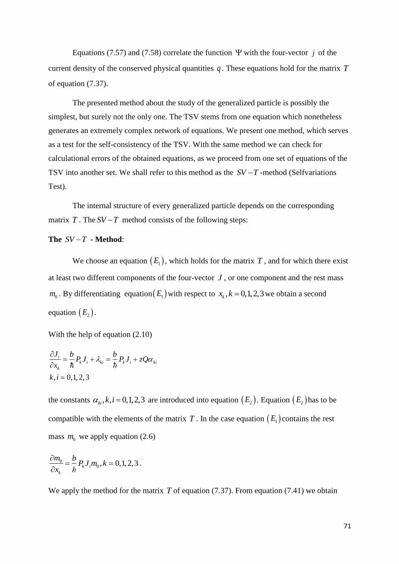
71

Equations (7.57) and (7.58) correlate the function with the four-vector j of the

current density of the conserved physical quantities q . These equations hold for the matrix T

of equation (7.37).

The presented method about the study of the generalized particle is possibly the

simplest, but surely not the only one. The TSV stems from one equation which nonetheless

generates an extremely complex network of equations. We present one method, which serves

as a test for the self-consistency of the TSV. With the same method we can check for

calculational errors of the obtained equations, as we proceed from one set of equations of the

TSV into another set. We shall refer to this method as the SV T -method (Selfvariations

Test).

The internal structure of every generalized particle depends on the corresponding

matrix T . The SV T method consists of the following steps:

The SV T - Method:

We choose an equation 1E , which holds for the matrix T , and for which there exist

at least two different components of the four-vector J , or one component and the rest mass

0m . By differentiating equation 1E with respect to , 0,1,2,3kx k we obtain a second

equation 2E .

With the help of equation (2.10)

, 0,1,2,3

ik i ki k i ki

k

J b bP J P J zQ

x

k i

the constants , , 0,1,2,3ki k i are introduced into equation 2E . Equation 2E has to be

compatible with the elements of the matrix T . In the case equation 1E contains the rest

mass 0m we apply equation (2.6)

00 , 0,1,2,3k i

k

m bP J m k

x

.

We apply the method for the matrix T of equation (7.37). From equation (7.41) we obtain

72

2 0J iJ . (7.59)

This equation contains the components 0 2,J J of the four-vector J . We differentiate equation

(7.59) with respect to , 0,1,2,3kx k , to obtain

2 2 0 0k k k k

b bP J zQ i P J zQ

and using equation (7.59) we have

2 0k kzQ izQ

and since 0zQ we get

2 0, 0,1,2,3k ki k . (7.60)

In equation (7.60) we insert successively 0,1,2,3k

For 0k we obtain

02 00 0i iT

which holds, since 02 00, 0T .

For 1k we get

12 10i

and since 10 01 , we get

12 01

2 2

01 21 0

i

which are equations (7.38).

For 2k we obtain

22 20

2 20

a ia

T ia

which holds for the matrix T , since 02 20, 0a T .

73

For 3k we have

32 30

32 03

i

i

which holds for the matrix T , since 32 030, 0 .

For the matrix we study it holds that τ 0 and n 0 and τ n 0 ,and therefore

plane is defined. From equations (7.32) we have

1

2

3

0

1

0

0

0

0

0

i

i

ε

ε

ε

. (7.61)


1

0 1 20 1

0

c

c ci ic

C ε ε . (7.62)

Equations (7.62) contains the components 0 1,ic c of the vector Cwith respect to the vector

basis 1 2,ε ε of the -plane. Considering that the vectors 1 2,ε ε are perpendicular to each

other, we obtain from equation (7.62)

1 0

2 1

ic

ic

ε C

ε C


1 0

0 12 0 2

ic

E icM

c c

ε C

ε C (7.63)

The material particle exists for 0J , hence from equation (7.41) we have

74

0 0J . (7.64)

From the equations (7.41) and (7.46) it follows that for 1 0c the 4-vectors J and C are

parallel, which is impossible in symmetry for the matrix T of our study. Therefore it is

1 0c (7.65)

for the symmetry of equation (7.37).


, , 0,1,2,32

ki i k k i

bc J c J k i


, , 0,1,2,32

ki i k k i

bzQ c J c J k i (7.66)

For 0, 1k i in equation (7.66) we have

01 1 0 0 12

bzQa c J c J

and because of 1 0J according to equation (7.41) we have

0 01

1

2J zQ

bc . (7.67)

Similarly for 2, 1k i in equation (7.66) we have

2 21

1

2J zQ

bc . (7.68)

Considering that 1 3 0J J according to equation (7.41), from equations (7.67) and (7.68)

we have

01

211

02

0

J zQbc

. (7.69)

Eq. (7.69) expresses the contribution of the charge Q to the 4-vector of momentum of the

material particle.

From equation (2.10) for 0k and taking into account equation

00 0 0zQT

75

we obtain

00 0

0

J bP J

x


0

0

zQ bP zQ

x

0

0 0

Q z bz Q P zQ

x x


0 0

0

b z bz PQ Q P zQ

x

0

0z

x


0 0c

and the equations (7.55) and (7.62), (7.63) written in the form

01

211

02

0

J zQbc

1

0

0

0

cC

P C J (7.70)

01

2

1

21

0

0

c bcj

2

1 0 1 0 0 1 00, 0, ,c m c iM c E icc M c

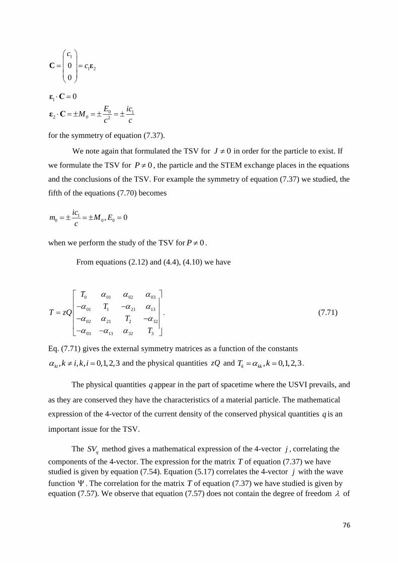
76

1 2

1

0

0

c

c

C ε

1

0 12 0 2

0

E icM

c c

ε C

ε C

for the symmetry of equation (7.37).

We note again that formulated the TSV for 0J in order for the particle to exist. If

we formulate the TSV for 0P , the particle and the STEM exchange places in the equations

and the conclusions of the TSV. For example the symmetry of equation (7.37) we studied, the

fifth of the equations (7.70) becomes

10 0 0, 0

icm M E

c

when we perform the study of the TSV for 0P .

From equations (2.12) and (4.4), (4.10) we have

0 01 02 03

01 1 21 13

02 21 2 32

03 13 32 3

T

TT zQ

T

T

. (7.71)

Eq. (7.71) gives the external symmetry matrices as a function of the constants

, , , 0,1,2,3ki k i k i and the physical quantities zQ and , 0,1,2,3k kkT k .

The physical quantities q appear in the part of spacetime where the USVI prevails, and

as they are conserved they have the characteristics of a material particle. The mathematical

expression of the 4-vector of the current density of the conserved physical quantities q is an

important issue for the TSV.

The qSV method gives a mathematical expression of the 4-vector j , correlating the

components of the 4-vector. The expression for the matrix T of equation (7.37) we have

studied is given by equation (7.54). Equation (5.17) correlates the 4-vector j with the wave

function . The correlation for the matrix T of equation (7.37) we have studied is given by

equation (7.57). We observe that equation (7.57) does not contain the degree of freedom of

77

equation (5.17), but only the degree of freedom . This is not a random fact valid for the

matrix we have studied, but is predicted by the next theorem:

Theorem 7.5

1. ΄΄The 4-vector j of the current density of the conserved physical quantities q of the

generalized particle is given by the equation

2bc

j J MC

(7.72)

where and the two degrees of freedom of the TSV and

0

1

2

3

0 0 0

0 0 0

0 0 0

0 0 0

T

T

T

T

01 02 03

01 21 13

02 21 32

03 13 32

0

0

0

0

M

the fundamental matrices and M of the TSV.

2. 2

0bc

J j MC

.΄΄ (7.73)

Proof. From equation (3.5) we have

P C J

and replacing the momentum P in equation (5.7) we have

2c b

j M J C J

2c b

j M J C

2c b

j MJ MC

. (7.74)

From equations (7.71) and (4.11), (4.28) we have

78

T zQ M

and from equation (2.13) we have

0zQ M J

and since 0zQ we have

0M J

0MJ J

and finally we get

MJ J (7.75)

From equations (7.74) and (7.75) we get equation (7.72). The equation (7.73) follows from

the equation (7.72) for 0J .

As we shall see next the relation 0J is valid for a large number of external

symmetry matrices. For these matrices Nr. 2.of theorem 7.5 is valid.


1

0 0 0 0

0 0 0

0 0 0 0

0 0 0 0

T

and with equation (7.41) we have 0J for the symmetry we have studied. Next from

equations (7.42) and (7.46), equation (7.57) follows from the relation (7.73).

We now prove the following corollary of theorem 7.5:

Corollary 7.4. ΄΄In flat spacetime the 4-vector j of the current density of the conserved

physical quantities q of the generalized particle is given by equation

2bc

j MC

.΄΄

Proof. From corollary 6.1 and equation (4.11) it follows that in flat spacetime we have 0

and therefore Nr. 2.of theorem 7.5 is true.

The next theorem 7.6 relates the four-vector J with the elements of the main

diagonal of the external symmetry matrix T .

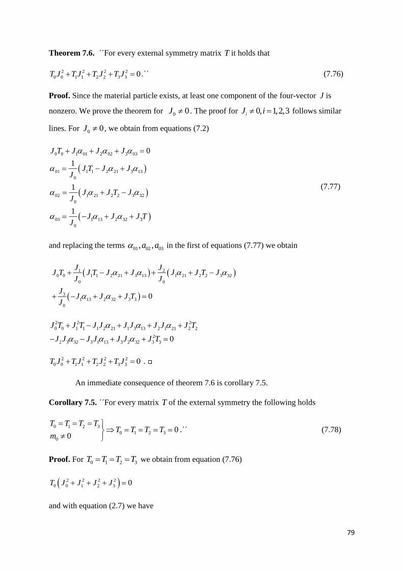
79

Theorem 7.6. ΄΄For every external symmetry matrix T it holds that

2 2 2 2

0 0 1 1 2 2 3 3 0T J T J T J T J .΄΄ (7.76)

Proof. Since the material particle exists, at least one component of the four-vector J is

nonzero. We prove the theorem for 0 0J . The proof for 0, 1,2,3iJ i follows similar

lines. For 0 0J , we obtain from equations (7.2)

0 0 1 01 2 02 3 03

01 1 1 2 21 3 13

0

02 1 21 2 2 3 32

0

03 1 13 2 32 3

0

0

1

1

1

J T J J J

J T J JJ

J J T JJ

J J J TJ

(7.77)

and replacing the terms 01 02 03, ,a a in the first of equations (7.77) we obtain

1 20 0 1 1 2 21 3 13 1 21 2 2 3 32

0 0

31 13 2 32 3 3

0

0

J JJ T J T J J J J T J

J J

JJ J J T

J

2 2 2

0 0 1 1 1 2 21 1 3 13 2 1 21 2 2

2

2 3 32 3 1 13 3 2 32 3 3 0

J T J T J J J J J J J T

J J J J J J J T

2 2 2 2

0 0 1 1 2 2 3 3 0T J T J T J T J .

An immediate consequence of theorem 7.6 is corollary 7.5.

Corollary 7.5. ΄΄For every matrix T of the external symmetry the following holds

0 1 2 3

0 1 2 3

0

00

T T T TT T T T

m

.΄΄ (7.78)

Proof. For 0 1 2 3T T T T we obtain from equation (7.76)

2 2 2 2

0 0 1 2 3 0T J J J J


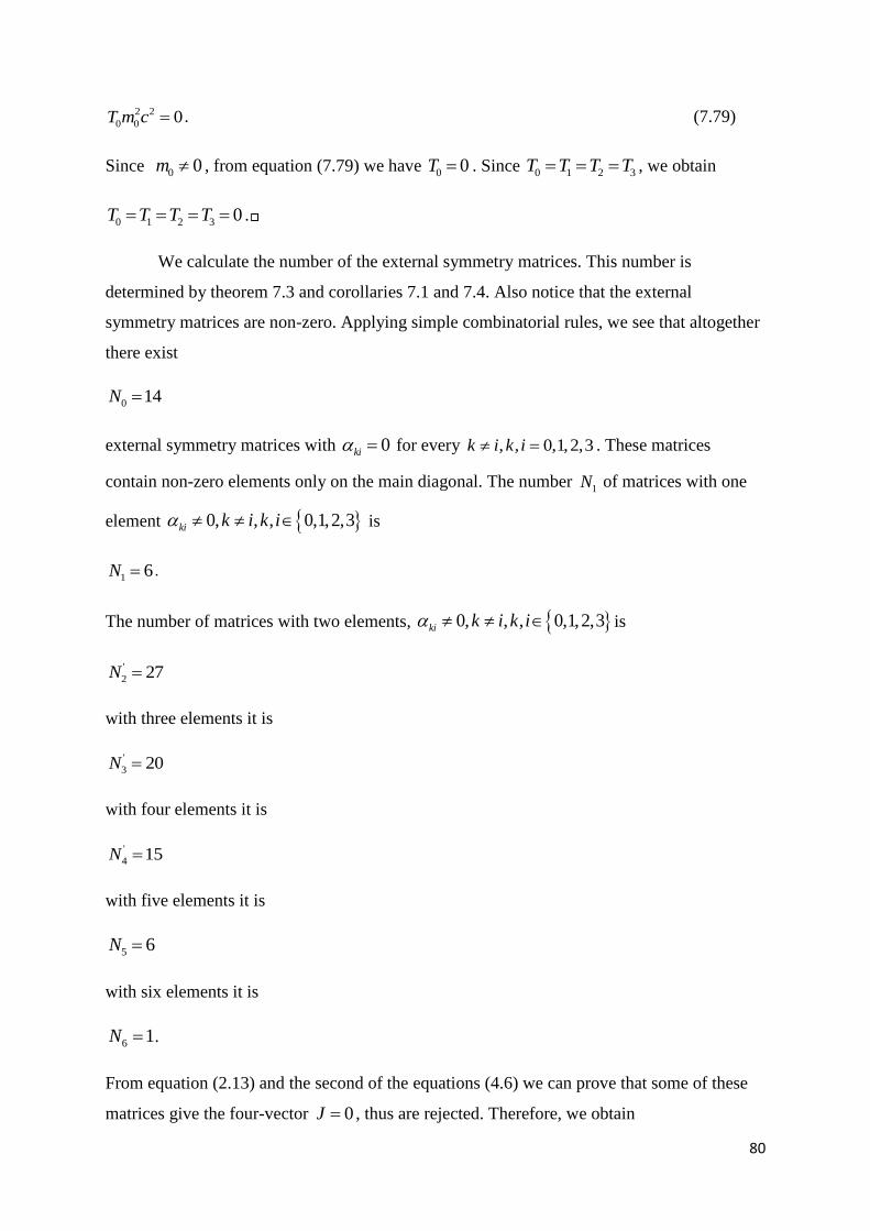
80

2 2

0 0 0T m c . (7.79)

Since 0 0m , from equation (7.79) we have 0 0T . Since 0 1 2 3T T T T , we obtain

0 1 2 3 0T T T T .

We calculate the number of the external symmetry matrices. This number is

determined by theorem 7.3 and corollaries 7.1 and 7.4. Also notice that the external

symmetry matrices are non-zero. Applying simple combinatorial rules, we see that altogether

there exist

0 14N

external symmetry matrices with 0ki for every , , 0,1,2,3k i k i . These matrices

contain non-zero elements only on the main diagonal. The number 1N of matrices with one

element 0, , , 0,1,2,3ki k i k i is

1 6N .

The number of matrices with two elements, 0, , , 0,1,2,3ki k i k i is

'

2 27N

with three elements it is

'

3 20N

with four elements it is

'

4 15N

with five elements it is

5 6N

with six elements it is

6 1N .

From equation (2.13) and the second of the equations (4.6) we can prove that some of these

matrices give the four-vector 0J , thus are rejected. Therefore, we obtain

81

0

1

'

2 2

'

3 3

'

4 4

5

6

14

6

4 24

8 12

12 3

6

1

N

N

N N

N N

N N

N

N

.

Thus the total number TN of external symmetry matrices is

0 1 2 3 4 5 6 66TN N N N N N N N . (7.80)

The matrix 0T is unique

1ON

and according to theorem 3.3 this matrix expresses the internal symmetry. Therefore, the total

number of the matrices of the internal and external symmetry predicted by the Law of

Selfvariations is

67OT O TN N N . (7.81)

There exist

16 50J TN N (7.82)

external symmetry matrices with different four-vectors , , ,J P C j .

We now prove for example that the following matrix

0 01 03

01 1 21 13

21 2

03 13 3

0

0 0

0

T

TT zQ

T

T

is not an external symmetry matrix. Applying theorem 7.3 for the above matrix we have

0 1 2 3 0T T T T

and therefore it takes the form

82

01 03

01 21 13

21

03 13

0 0

0

0 0 0

0 0

T zQ


1 01 3 03

0 01 2 21 3 13

1 21

0 03 1 13

0

0

0

0

J J

J J J

J

J J

and since

01 03 13 21 0

we have

0 1 2 3 0J J J J

which is impossible since there is no material particle in this case.

We present now a notation for the matrices of the external symmetry. In every matrix

T we use an upper and a lower index. As lower indices we use the pairs

, , , , 0,1,2,3k i k i k i of the constants 0ki , which are nonzero. These indices, which

appear always in pairs, are placed in the order of the following constants:

01 02 03 32 13 21, , , , , , which are nonzero. As upper indices we use the indices of the

nonzero elements of the main diagonal, in the following order: 0 1 2 3, , ,T T T T . For example, the

matrix T given in equation (7.37) is denoted as 1

0121T .

With this notation, the external symmetry matrices are given from the following seven

sets :

83

0 1 2 3 01 02 03 12 13 23 012 013 023 123

0

01 02 03 23 13 12

1 01 02 03 32 13 21

0 0 0 3 2 1

2 0102 0103 0103 0203 0203 3213 3213 3221 3221 1321 13210102

1 1

0113 0113 0121 01

, , , , , , , , , , , , ,

, , , , ,

, , , , , , , , , , , ,

, , ,

T T T T T T T T T T T T T T

T T T T T T

T T T T T T T T T T T T

T T T T

2 2 3 3

21 0232 0232 0221 0221 0332 0332 0313 0313

0 1 2 3

3 010203 010203 011321 011321 023221 023221 033213 033213

010221 010313 020332 321321

4 01023213 01033221 02031321

5 01020332

, , , , , , , ,

, , , , , , , ,

, , ,

, ,

T T T T T T T T

T T T T T T T T

T T T T

T T T

T

21 0102033213 0102031321 0102321321 0103321321 0203321321

6 010203321321

, , , , ,T T T T T

T

. (7.83)

We note that in the 4-dimensional spacetime the matrix 321321T of the set

3 is discarded by

the SV T method. The application of the SV T method to set 5 is of particular interest,

as we will see in chapter 14.

The internal symmetry expresses the spontaneous isotropic STEM emission from a

material particle because of the selfvariations. The external symmetry emerges when the

material particle interacts via the USVI with other material particles and this is equivalent

with the destruction of the spacetime isotropy. The rest mass of the material particle and of

the STEM in the first case, as well as the rest mass which stems from the USVI in the second

case, is given by the equations (2.7) and (2.8). The equations (7.69) and (7.70)

01

211

01

1

211

02

0

0

02

0

0 0

J J Q zQbc

cP P Q zQ

bc

(7.84)

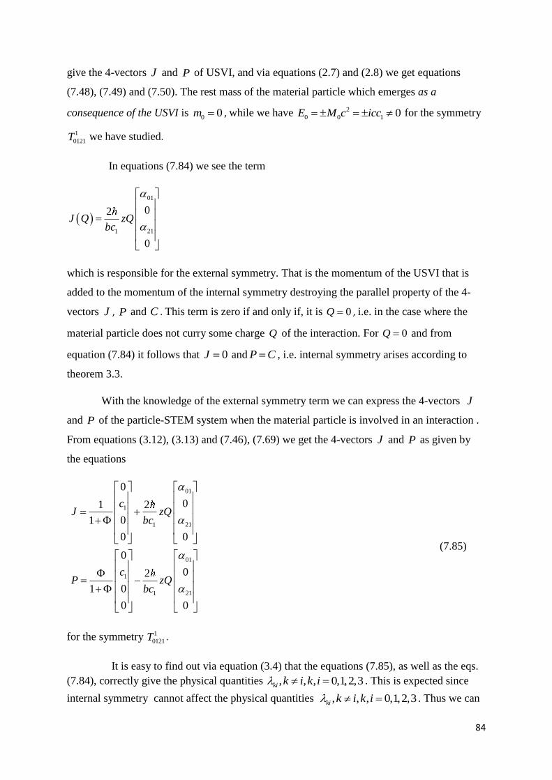
84

give the 4-vectors J and P of USVI, and via equations (2.7) and (2.8) we get equations

(7.48), (7.49) and (7.50). The rest mass of the material particle which emerges as a

consequence of the USVI is 0 0m , while we have 2

0 0 1 0E M c icc for the symmetry

1

0121T we have studied.

In equations (7.84) we see the term

01

211

02

0

J Q zQbc

which is responsible for the external symmetry. That is the momentum of the USVI that is

added to the momentum of the internal symmetry destroying the parallel property of the 4-

vectors J , P and C . This term is zero if and only if, it is 0Q , i.e. in the case where the

material particle does not curry some charge Q of the interaction. For 0Q and from

equation (7.84) it follows that 0J and P C , i.e. internal symmetry arises according to

theorem 3.3.

With the knowledge of the external symmetry term we can express the 4-vectors J

and P of the particle-STEM system when the material particle is involved in an interaction .

From equations (3.12), (3.13) and (7.46), (7.69) we get the 4-vectors J and P as given by

the equations

01

1

211

01

1

211

0

01 2

01

0 0

0

02

01

0 0

cJ zQ

bc

cP zQ

bc

(7.85)

for the symmetry 1

0121T .

It is easy to find out via equation (3.4) that the equations (7.85), as well as the eqs.

(7.84), correctly give the physical quantities , , , 0,1,2,3ki k i k i . This is expected since

internal symmetry cannot affect the physical quantities , , , 0,1,2,3ki k i k i . Thus we can

85

calculate the constants , , , 0,1,2,3ki k i k i and the physical quantities , 0,1,2,3kT k

either through equations (7.84) or through equations (7.85). The TSV equations are valid for

equations (7.84) as well as for equations (7.85).

For 0Q from equations (7.85) we have

1

1

0

1

01

0

0

01

0

cJ

cP

that is we get equations (3.12) and (3.13) with 0 2 3 10, 0c c c c . Therefore when the

material particle does not interact with other material particles, internal symmetry arises in

both cases. Also the equations (7.85) give the rest mass

00

1

Mm

of the material particle, as follows from equation (2.7). The interaction (USVI) in which the

material particle is involved does not affect its rest mass, as given by equation (3.10).

Every external symmetry has its own 4-vector C and its own term J Q . In every

external symmetry there exist equations corresponding to equations (7.84)

P Q C J Q

for the USVI particle and to equations (7.85)

1

1

1

J C J Q

P C J Q

(7.86)

for the material particle.

From equations (2.7) and (2.8) another important conclusion follows. In internal

symmetry the material particle and STEM exchange roles if mutually exchanged

0 0 00 1 2 3 0 0 0 1 2 3 02, , , , , , , , , , , 0,1,2,3k k

k k

m E Eb bJ J J J m P m P P P P J E k

x c x

. (7.87)

86

According to theorem 3.3 in internal symmetry the 4-vectors J and P are parallel which

implies that they have the same form. Hence the mutual exchange (7.87) has no consequences

in internal symmetry. If we assume that one of the 4-vectors J and P corresponds to the

material particle, then the other corresponds to STEM. This fact can also be seen from

equations (3.9)-(3.13) of the theorem 3.3, which can be written in an equivalent form.

* *

0 0 1 1 2 2 3 3 0 0 1 1 2 2 3 3

*

00 *

00 *

*

*

*

1 1exp exp

1

1

, 0,1,2,31

, 0,1,2,31

ii

ii

b bc x c x c x c x K c x c x c x c x

K

Mm

ME

cJ i

cP i

. (7.88)

The different appearance of the 4-vectors J and P , and the rest masses 0m and 0

2

E

c in

theorem 3.3 is superficial. Their form depends on whether we use equation or eq. * to

write them.

In external symmetry the mutual exchange (7.87) is not enough for the role exchange

of the material particle and STEM. From equations (7.85) it follows that the role exchange of

the material particle and STEM via equations (7.88) can only be realized with the

simultaneous change of sign of the charge Q Q Q .

Combining equations (2.10), (3.5) and (4.4), and with equation (2.13) we have

, , 0,1,2,3

0

ik i ki

k

J bP J zQ k i

x

J P C

TJ

. (7.89)

It is easy to find out that the TSV can be formulated starting from eqs. (7.89). The equations

(7.89) give the Selfvariations of the 4-vectors J and P . They are more general than equation

(2.6) since they give the TSV equations independent of whether the rest mass 0m of the

material particle is zero or not. We have chosen to start the formulation of the TSV from

equation (2.6), which gives the equations of the TSV for 0 0m , for the reason that there is

87

no other way to approach equations (7.89). Moreover their physical content would not be

clear.

Based on the theorems of the TSV we can study all external symmetry matrices. The

combination of methods SV M and qSV with which we studied the symmetry 1

0121T can be

applied to any external symmetry of the set 1 2 3 4 5 6 . We will also

apply this method in chapter 9 in our study of the symmetries of the set 3 . Equally well we

can study any external symmetry with a second method based on equations (7.20), (7.2),

(4.6), on the SV T method, on equation (7.17), on corollary 5.1 and on corollary 5.3. This

second method we present in the chapters 12, 13, 14 and 15 where we study the symmetries

of the sets 1 ,

4 , 5 and

6 . Generally we can say that the first method deepens the

understanding of the relations between the physical quantities which emerge from the TSV.

With the second method the study of the external symmetry is completed faster and more

elegant.

8. THE SET 0

8.1. Introduction

In this chapter we study the T matrices, which have all their elements equal to zero,

except the elements on the main diagonal. Thus we study matrices of the form

0

1

2

3

0 0 0

0 0 0

0 0 0

0 0 0

T

TT zQ zQ

T

T

i.e. the elements of the set 0 .

In the symmetries of the set 0 the rest mass of the particle which accompanies the

USVI may be non-zero. In all external symmetries this property can be found only in the sets

0 and 1 .

88

8.2. The Symmetries T=zQΛ


0

1

2

3

0 0 0

0 0 0

0 0 0

0 0 0

T

TT zQ zQ

T

T

. (8.1)

From equations (4.28) ,(7.3) and (8.1) we have

0

0

M

N

. (8.2)

The matrices M and N are zero; as a consequence the matrices of the symmetries T zQ

share common properties, which we shall study in the following.

According to corollary 7.4 , at least one of the diagonal elements of the matrices of

equation (8.1) is zero. Also they cannot be all zero, since in the case of the external symmetry

it holds that 0T . Therefore, there is a number of

0

4 4 414

1 2 3N

different matrices for which the relation T zQ holds.

A common characteristic for the 14 kinds of symmetries T zQ is that τ 0 , and

therefore the plane is not defined. Similarly, the vectors 1 2 3, ,ε ε ε of equations (7.32) are

not defined.

A fundamental characteristic of the symmetries T zQ is that the four-vector j of

the conserved physical quantites q vanishes. Combining the first of equations (8.2) with


0j . (8.3)

Therefore, in the part of spacetime occupied by the generalized particle, there is no flow of

conserved physical quantities q .

89

Another common characteristic is that the rest mass 0m of the material particle can

be diferent from zero

0 00 0m m (8.4)

for all 14 matrices of the symmetry. The form of the four-vector J is different for each matrix

of the symmetry.

We calculate now the four-vector of momentum J of the matrix 12T . According to

our notation we have

112

2

1 2

0 0 0 0

0 0 0

0 0 0

0 0 0 0

0

TT zQ

T

TT

. (8.5)

From equation (2.13), and since 1 2 0TT , 0 3 0T T , we obtain for the four-vector

J , in the form

0

3

0

0

J

J

J

. (8.6)

Combining equations (2.7) and (8.6), we obtain for the rest mass 0m the equation

2 2 2 2

0 0 3m c J J . (8.7)

We apply now the SV T method :

We differentiate equation (8.7) with respect to , 0,1,2,3kx k and taking into account

equations (2.6), (2.10) and (4.4) we obtain

2 2

0 0 0 0 3 3 3k k k k k

b b bP m c J P J zQ J P J zQ


0 0 3 3 0k kzQJ zQJ

90

and since 0zQ , we have

0 0 3 3 0, 0,1,2,3k kJ J k . (8.8)

We insert successively 0,1,2,3k into equation (8.8), hence:

For 0k we have

0 0 3 03 0J T J

which holds since for the matrix 12T it is 0 03 0T .

For 1k we have

0 10 3 13 0J J

which holds since for the matrix 12T it is 10 13 0 .

For 2k we have

0 20 3 23 0J J

which holds since for the matrix 12T it is 20 32 0 .

For 3k we have

0 30 3 3 0J J T

which holds since for the matrix 12T it is 30 3 0T .

According to the proof of equation (8.7) it is possible that 0 0J or 3 0J , but it is

not possible that 0 3 0J J , since in this case the material particle does not exist. Therefore

from equation (8.7) we conclude that

0 0 3 00 0m m J iJ . (8.9)

Simirarly we can prove that relations analogous to relation (8.10), hold for all matrices of the

symmetry T zQ .

For the matrix 12T it is 1 0T . Therefore the part of spacetime occupied by the

generalized particle in the symmetry 12T is curved, according to corollary 6.2.

91

Because of equation (8.3) the wave equation (5.17) holds identically 0 0 . Therefore for

the symmetries T zQ the study of the wave behavior of matter is done via equation (5.3).

Starting from equation (8.7) and applying the same method of proof as for equations

(4.19) and (4.20) we obtain

0 0

dJ dQJ

dx Qdx (8.10)

0 0

dP dQJ

dx Qdx (8.11)

for the symmetry 12T . From equations (8.6) and (8.10) we obtain

00

0 0

33

0 0

dJ dQJ

dx Qdx

dJ dQJ

dx Qdx


0 0

3 3

0 3

0 3

, 0,0

, constants

J Q

J Q

. (8.12)

Thus the four-vector J is given by equation

0

3

0 3

0 3

0

0

, 0,0

, constants

J J Q Q

(8.13)

as implied by equation (8.6). Therefore, for the symmetry 12T the momentum of the material

particle is proportional to the charge Q . This feature is a common characteristic for all

matrices of the symmetry T zQ .

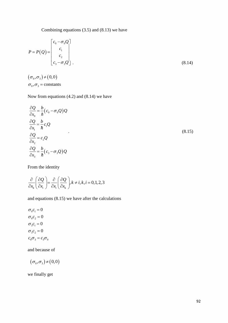
92

Combining equations (3.5) and (8.13) we have

0 0

1

2

3 3

0 3

0 3

, 0,0

, constants

c Q

cP P Q

c

c Q

. (8.14)

Now from equations (4.2) and (8.14) we have

0 0

0

1

1

2

2

3 3

3

Q bc Q Q

x

Q bc Q

x

Qc Q

x

Q bc Q Q

x

. (8.15)

From the identity

, , , 0,1,2,3k i i k

Q Qk i k i

x x x x

and equations (8.15) we have after the calculations

0 1

0 2

3 1

3 2

0 3 3 0

0

0

0

0

c

c

c

c

c c

and because of

0 3, 0,0

we finally get

93

1 2

0 3 3 0

0c c

c c

. (8.16)


0 3

0 0

0

3 3

3

,Q Q x x

Q bc Q Q

x

Q bc Q Q

x

. (8.17)


0

012 0 0 3 3

0 3 3 0

0

1

1 exp

0

cQ

bK c x c x

c c

(8.18)

3

312 0 0 3 3

0 3 3 0

3

1

1 exp

0

cQ

bK c x c x

c c

(8.19)

where 12 12, 0K K constant. For

0 3 0 the equations (8.18) and (8.19) are equivalent,

because of the second equation of (8.16).

From equation (8.14) and the first equation of (8.16) we have

0 0

3 3

0

0

c Q

P P Q

c Q

. (8.20)

From equation (3.5) and the first equation of (8.16) we have

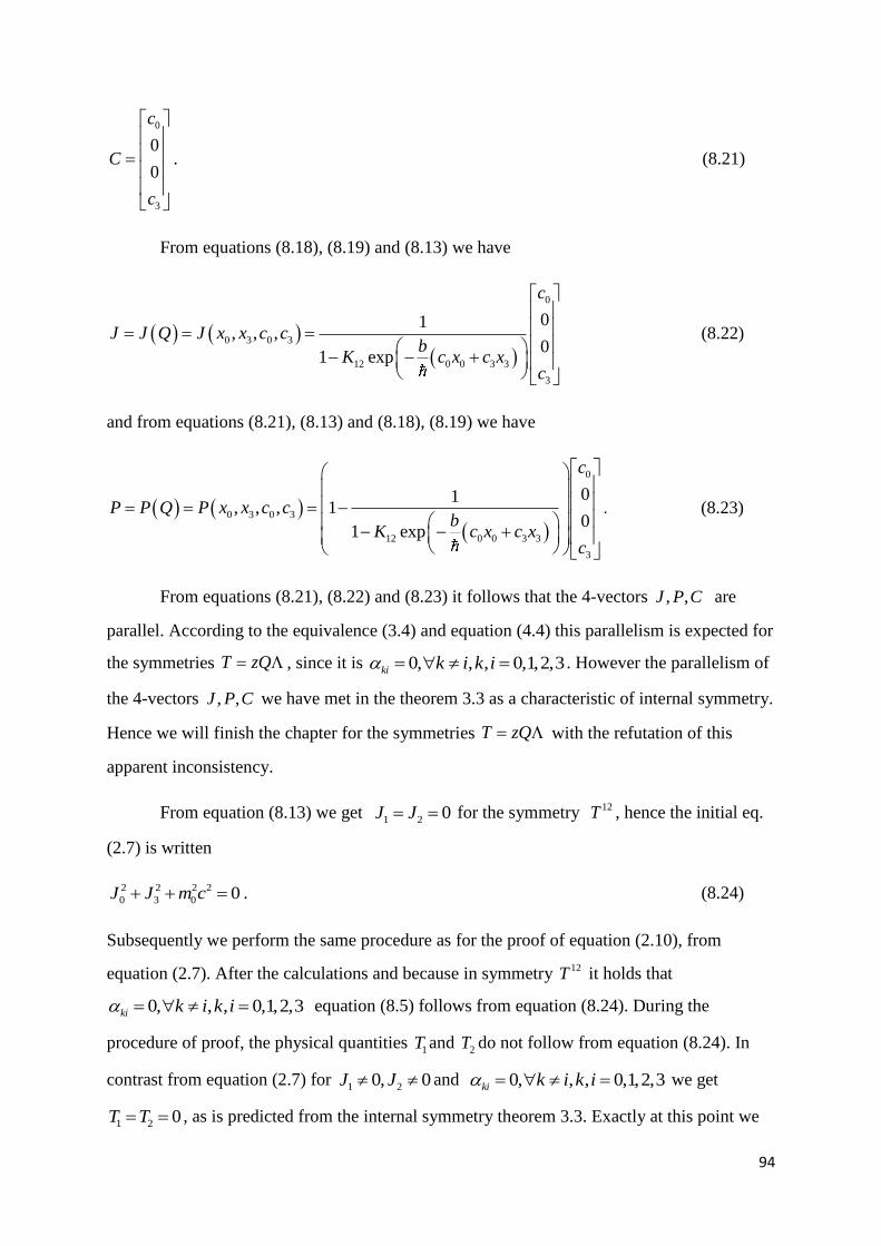
94

0

3

0

0

c

C

c

. (8.21)

From equations (8.18), (8.19) and (8.13) we have

0

0 3 0 3

12 0 0 3 3

3

01, , ,

01 exp

c

J J Q J x x c cb

K c x c xc

(8.22)

and from equations (8.21), (8.13) and (8.18), (8.19) we have

0

0 3 0 3

12 0 0 3 3

3

01, , , 1

01 exp

c

P P Q P x x c cb

K c x c xc

. (8.23)

From equations (8.21), (8.22) and (8.23) it follows that the 4-vectors , ,J P C are

parallel. According to the equivalence (3.4) and equation (4.4) this parallelism is expected for

the symmetries T zQ , since it is 0, , , 0,1,2,3ki k i k i . However the parallelism of

the 4-vectors , ,J P C we have met in the theorem 3.3 as a characteristic of internal symmetry.

Hence we will finish the chapter for the symmetries T zQ with the refutation of this

apparent inconsistency.

From equation (8.13) we get 1 2 0J J for the symmetry 12T , hence the initial eq.

(2.7) is written

2 2 2 2

0 3 0 0J J m c . (8.24)

Subsequently we perform the same procedure as for the proof of equation (2.10), from

equation (2.7). After the calculations and because in symmetry 12T it holds that

0, , , 0,1,2,3ki k i k i equation (8.5) follows from equation (8.24). During the

procedure of proof, the physical quantities 1T and

2T do not follow from equation (8.24). In

contrast from equation (2.7) for 1 20, 0J J and 0, , , 0,1,2,3ki k i k i we get

1 2 0T T , as is predicted from the internal symmetry theorem 3.3. Exactly at this point we

95

find the differences of the symmetries T zQ with internal symmetry. In internal

symmetry it is 0 1 2 3 0T T T T , and according to corollary 6.1 the part of spacetime

occupied by the generalized particle may be a plane. Moreover space is isotropic, in the part

of spacetime occupied by the generalized particle. The momentum vectors J , P and C are 3-

dimensional, and it is not possible to let vanish some component 1 2 3, ,J J J of the momentum

from equation (2.7), with an appropriate rotation of the reference system we use. There is a

very specific inertial reference frame in which 1 2 3 0J J J ([5], chapter 5.3). In contrast

with the symmetries T zQ spacetime is curved as implied by the corollary 6.2. Moreover

in symmetries T zQ space is intensely anisotropic, in the part of spacetime which is

occupied by the generalized particle. According to equations (8.21), (8.22) and (8.23) the

momentums C , J and P in symmetry 12T are 1-dimensional, towards the direction of the

axis 3x z . The intense anisotropy of space, in the part of spacetime which is occupied by

the generalized particle, is a basic characteristic of the symmetry T zQ . This anisotropy

varies for the symmetries of the set 1 in equation (7.83). One symmetry T zQ is

characterized by the symmetries of the 4-vector J which are absend in the equation (2.7). For

symmetry 12T the components are 1J and

2J .


2 2 2 2 2

0 3 0

0 3

0

, 0,0

Q m c

. (8.25)

Equation (8.25) gives the contribution of charge Q to the rest mass 0m of the material particle.

We now calculate the distribution of the total rest mass 0M of the generalized particle

between the material particle and STEM. From equations (8.22) and (8.24) we have

2 22 20 302

12 0 0 3 3

0

1 exp

c cm c

bK c x c x


96

2 22 2002

12 0 0 3 3

0

1 exp

M cm c

bK c x c x

and finally we get

00

12 0 0 3 31 exp

Mm

bK c x c x

(8.26)

Analogous from equations (8.23), (2.8), and (3.5) we have

2

0 12 0 0 3 3

0

12 0 0 3 3

exp

1 exp

bM c K c x c x

Eb

K c x c x

(8.27)

Equations (8.26) and (8.27) give the distribution of rest mass 0M between the material

particle and STEM. The study of the remaining 13 symmetries T zQ is done in the same

way as the one we demonstrated for symmetry 12T .

We now set 12K K in equations (8.22) and (8.23), where K the constant of

equation (3.9). Comparing equations (8.22), (8.23) and (3.9), (3.12), (3.13) we come to the

conclusion that the external symmetry 12T can emerge from the internal symmetry for

1 2 0J J . This can occur when an external cause blocks the emmision of STEM along the

axes 1x and

2x . In this way the isotropic emmision of the internal symmetry is converted into

the anisotropic external symmetry 12T . In general the following corollary of theorem 3.3

holds:

Corollary 8.1 : ΄΄The external symmetry T zQ can emerge from the internal symmetry

when the components of the momentum J of the material particle are in less than four axes

, 0,1,2,3ix i . These axes define the kind of external symmetry T zQ that results.΄΄

We present the method which can produce the symmetry 12T from internal symmetry.

We consider a case where an external cause can block the STEM emission in external

symmetry, on the plane defined by the two axes 1x and

2x . In this case we have

1 2 0P P . (8.28)

97

Now from equations (3.13), (3.12) and (8.28) we have

1 2

1 2

0

0

c c

J J

. (8.29)

From the combination of equations (8.28), (8.29) with equations (3.12), (3.13), (3.10), (3.11)

there arise the corresponding equations (8.22), (8.23), (8.26), (8.27) with 12K K .

Using function of equation (3.9) for 1 2 0c c , and

12K K equations (8.22),

(8.23), (8.26) and (8.27) are written in the form

1 2

, i 0,1,2,31

0

ii

cJ

c c

(8.30)

1 2

, i 0,1,2,31

0

ii

cP

c c

(8.31)

00

1 2

1

0

Mm

c c

(8.32)

2

00

1 2

1

0

M cE

c c

. (8.33)

Corollary 8.1 gives us a mechanism through which the symmetry T zQ can

emerge. The external cause is necessary, since the internal symmetry expresses the

spontaneous isotropic emmision of STEM due to the selfvariations.



and the conclusions of the TSV.

From the combination of equations (3.5), (5.3) and (8.30), (8.31) we get

0

0 1

1

cb

x

b

C

. (8.34)

By setting

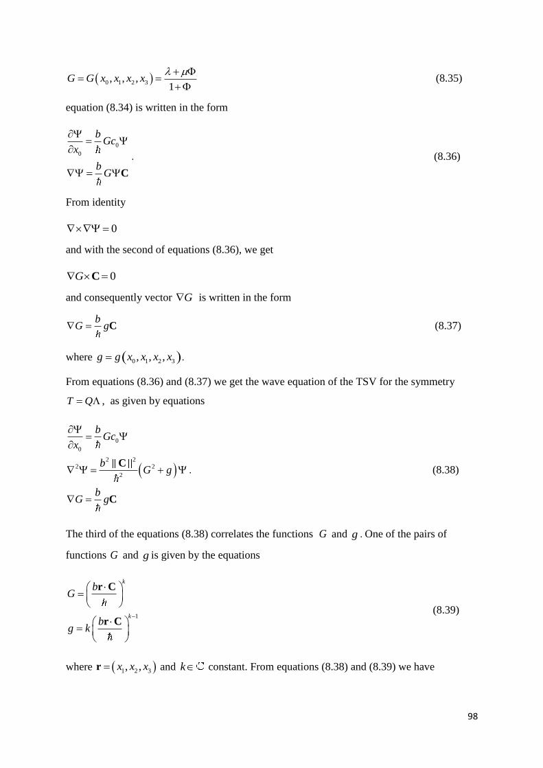
98

0 1 2 3, , ,1

G G x x x x

(8.35)

equation (8.34) is written in the form

0

0

bGc

x

bG

C

. (8.36)

From identity

0

and with the second of equations (8.36), we get

0G C

and consequently vector G is written in the form

bG g C (8.37)

where 0 1 2 3, , ,g g x x x x .

From equations (8.36) and (8.37) we get the wave equation of the TSV for the symmetry

T Q , as given by equations

0

0

2 22 2

2

bGc

x

bG g

bG g

C

C

. (8.38)

The third of the equations (8.38) correlates the functions G and g . One of the pairs of

functions G and g is given by the equations

1

k

k

bG

bg k

r C

r C (8.39)

where 1 2 3, ,x x xr and k constant. From equations (8.38) and (8.39) we have

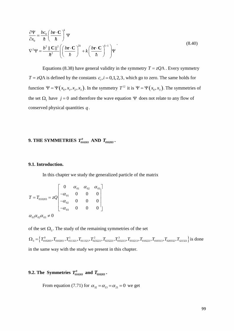
99

0

0

2 12 22

2

k

k k

bc b

x

b b bk

r C

rC C r C. (8.40)

Equations (8.38) have general validity in the symmetry T zQ . Every symmetry

T zQ is defined by the constants , 0,1,2,3ic i , which go to zero. The same holds for

function 0 1 2 3, , ,x x x x . In the symmetry 12T it is 0 3,x x . The symmetries of

the set 1 have 0j and therefore the wave equation does not relate to any flow of

conserved physical quantities q .

9. THE SYMMETRIES 0

010203T AND 010203

T .

9.1. Introduction.

In this chapter we study the generalized particle of the matrix

01 02 03

01

010203

02

03

01 02 03

0

0 0 0

0 0 0

0 0 0

0

T T zQ

of the set 3 . The study of the remaining symmetries of the set

0 1 2 3

3 010203 010203 011321 011321 023221 023221 033213 033213 010221 010313 020332 321321, , , , , , , , , , ,T T T T T T T T T T T T is done

in the same way with the study we present in this chapter.

9.2. The Symmetries 0

010203T and 010203T .

From equation (7.71) for 32 13 21 0 we get

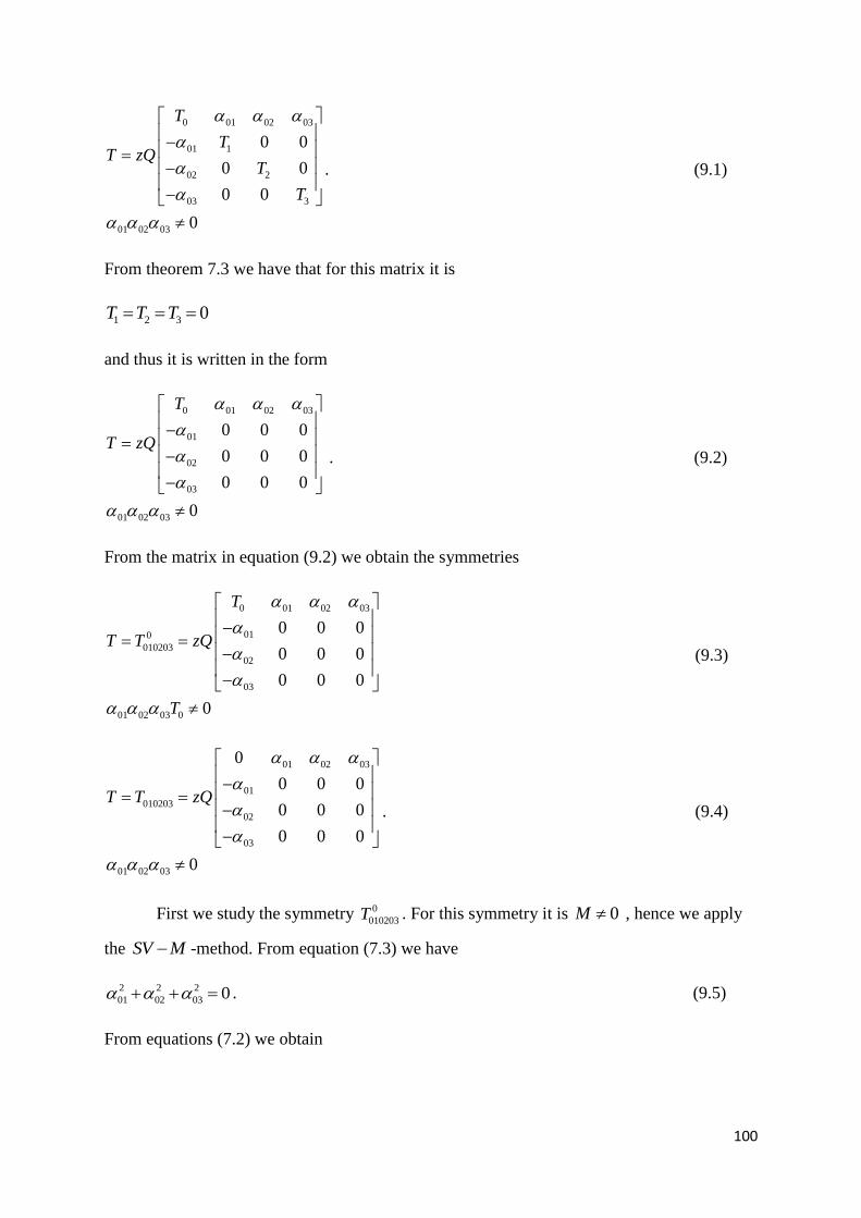
100

0 01 02 03

01 1

02 2

03 3

01 02 03

0 0

0 0

0 0

0

T

TT zQ

T

T

. (9.1)

From theorem 7.3 we have that for this matrix it is

1 2 3 0T T T

and thus it is written in the form

0 01 02 03

01

02

03

01 02 03

0 0 0

0 0 0

0 0 0

0

T

T zQ

. (9.2)

From the matrix in equation (9.2) we obtain the symmetries

0 01 02 03

010

010203

02

03

01 02 03 0

0 0 0

0 0 0

0 0 0

0

T

T T zQ

T

(9.3)

01 02 03

01

010203

02

03

01 02 03

0

0 0 0

0 0 0

0 0 0

0

T T zQ

. (9.4)

First we study the symmetry 0

010203T . For this symmetry it is 0M , hence we apply

the SV M -method. From equation (7.3) we have

2 2 2

01 02 03 0 . (9.5)


101

0 0 1 01 2 02 3 03

0 01

0 02

0 03

0

0

0

0

J T J J J

J

J

J

and since 01 02 03 0 and 0 0T we have

0

1 01 2 02 3 03

0

0

J

J J J

. (9.6)

From the second of the equations (4.6), and for , , 0,1,2 , 0,1,3 , 0,2,3 , 1,2,3i we

obtain

0 12 2 01 1 20

0 13 3 01 1 30

0 23 3 02 2 30

1 23 3 12 2 31

0

0

0

0

J J J

J J J

J J J

J J J

2 01 1 02

3 01 1 03

3 02 2 03

0

0

0

J J

J J

J J

. (9.7)

From equations (9.6), (9.7), and since it holds that 01 02 03 0a a a , we have

0

022 1

01

031

01

0J

J J

J J

. (9.8)

From equations (9.8) we obtain the four-vector J J Q

02

1

01

03

01

1

0

1

0

J J Q J

J

(9.9)

102


01 02 03

01

02

03

0

0 0 0

0 0 0

0 0 0

M

(9.10)

2 2 2

01 02 03

2

2 01 01 02 01 03

2

01 02 02 02 03

2

01 03 02 03 03

0 0 0

0

0

0

M


2

01 01 02 01 032

2

01 02 02 02 03

2

01 03 02 03 03

0 0 0 0

0

0

0

M

. (9.11)

From the first of the equations (7.14) and the equation (9.11), we get after the calculations

1 01 2 02 3 03 0c c c . (9.12)

From the first of the equations (4.6), and for , , 0,1,2 , 0,1,3 , 0,2,3 , 1,2,3i we

obtain

0 12 2 01 1 20

0 13 3 01 1 30

0 23 3 02 2 30

1 23 3 12 2 31

0

0

0

0

c c c

c c c

c c c

c c c

2 01 1 02

3 01 1 03

3 02 2 03

0

0

0

c c

c c

c c

. (9.13)


022 1

01

033 1

01

c c

c c

. (9.14)

103

From equations (9.14) we obtain the four-vector C

0

1

021

01

031

02

0 0

c

c

cC

c

c

. (9.15)

From equation (3.5) and equations (9.9) and (9.15) we obtain the four-vector P P Q

0

1 1

021 1

01

031 1

01

c

c J

c JP P Q

c J

. (9.16)

With the knowledge of the four-vectors , ,J P C we can calculate the rest masses

00 02, ,E

m Mc

of the material which emerges as a concequence of the USVI. From equations

(2.7) and (9.9) we get

2 2

2 2 2 02 030 1

01 01

1m c J

and using equation (9.5) we obtain

0 0m . (9.17)


0 0E icc . (9.18)

For the proof of equation (9.18) we used also equation (9.5). From equations (3.6) and (9.15)

we have

0 0c iM c . (9.19)

104

The vector τ vanishes

32

13

21

0

0

0

τ

and thus the plane is not defined. For the same reason it also holds that μ 0 . On the

contrary the vector n is nonzero

01

02

03

0

0

0

n . (9.20)

From equations (9.9),(9.15) and (9.16) we see that the vectors , , J P C are parallel to the

vector n . From equivalence (3.4) we obtain

, , , 0,1,2,32

ki i k k i

bc J c J k i k i


2

ki i k k i

bzQ c J c J

and for 0, 0,1,2,3k i we obtain

01 1 0 0 1

02 2 0 0 2

03 3 0 0 3

2

2

2

bzQ c J c J

bzQ c J c J

bzQ c J c J


001 1

002 2

003 3

2

2

2

bczQ J

bczQ J

bczQ J

and solving with respect to 1 2 3, ,J J J we obtain

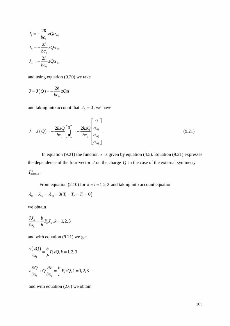
105

1 01

0

2 02

0

3 03

0

2

2

2

J zQbc

J zQbc

J zQbc

and using equation (9.20) we take

0

2Q zQ

bc J J n

and taking into account that 0 0J , we have

01

020 0

03

0

02 2zQ zQJ J Q

bc bc

n. (9.21)

In equation (9.21) the function z is given by equation (4.5). Equation (9.21) expresses

the dependence of the four-vector J on the charge Q in the case of the external symmetry

0

010203T .

From equation (2.10) for 1,2,3k i and taking into account equation

11 22 33 1 2 30 0T T T

we obtain

, 1,2,3kk k

k

J bP J k

x


, 1, 2,3k

k

zQ bP zQ k

x

, 1,2,3k

k k

Q z bz Q P zQ k

x x


106

, 1,2,3k k

k

b z bz P Q Q P zQ k

x

0, 1,2,3k

zk

x


1 2 3 0c c c


0

0

0

01

020

03

0

0

0

0

0

0 2

0

0

c

C

c

c

zQP P Q C J Q

bc

(9.22)

for the four-vectors C and P .




For the matrix 0

010203T it is 0M therefore we apply the qSV - method for the

determination of the four-vector j . For , , 0,1,2 , 0,1,3 , 0,2,3 , 1,2,3i in equation

(7.51) we get

0 12 2 01 1 20

0 13 3 01 1 30

0 23 3 02 2 30

1 23 3 12 2 31

0

0

0

0

j j j

j j j

j j j

j j j

and considering the elements of the matrix 0

010203T , we obtain

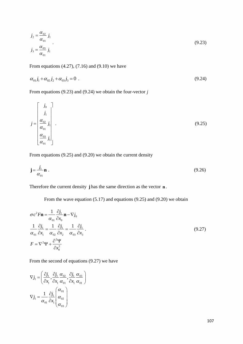
107

022 1

01

033 1

01

j j

j j

. (9.23)


01 1 02 2 03 3 0j j j . (9.24)

From equations (9.23) and (9.24) we obtain the four-vector j

0

1

021

01

031

01

j

j

jj

j

. (9.25)

From equations (9.25) and (9.20) we obtain the current density

1

01

j

j n . (9.26)

Therefore the current density j has the same direction as the vector n .

From the wave equation (5.17) and equations (9.25) and (9.20) we obtain

10

01 0

1 1 1

01 1 02 2 03 3

22

2

0

2 1

1 1 1

cj

jx

j j j

x x x

Fx

F

n n

. (9.27)

From the second of equations (9.27) we have

02 031 1 11

1 1 01 1 01

01

11 02

01 1

03

, ,

1

j j jj

x x x

jj

x

108


11

01 1

1 jj

x

n . (9.28)


2 2 2101 02 032

01 1

1 j

x

j


0 j . (9.29)

Combining the continuity equation (5.6) with equation (9.29) we obtain

0

0

0j

x

. (9.30)

Therefore the charge density 0j i c does not depend on time in the symmetry we study.

Combining equations (5.3), (9.9) and (9.16) we have

0

0

01

01 02

, , , 0,0

bc

x

cbJ

n . (9.31)

Let us remind that the parameters , appearing in equation (9.31) express the two degrees

of freedom of the TSV.

Setting

00 1 2 3 1

01 02

, , ,c

G G x x x x J

(9.32)

equation (9.31) is written in the form

0

0

bc

x

bG

n

. (9.33)

From identity

109

0

and the second of equations (9.33) we get

0G n

and, therefore, the vector G is written as

bG g n (9.34)

where 0 1 2 3, , ,g g x x x x .

From the second of equations (9.33) we get

2 bG G n

and with the second of equations (9.33), and equation (9.34) we get

2

2 2

2

bG g n n n

2

2 2

2

2bG g n


2

2 2 2 2 2

01 02 032

bG g

and with equation (9.5) we finally get

2 0 . (9.35)

In the symmetry 0

010203T the wave function of the TSV satisfies the Laplace equation. The

first of equations (9.33) and equation (9.35)

0

0

2 0

bc

x

(9.36)

constitute the wave function of the TSV for the symmetry 0

010203T .

From equation (9.25) it follows that the 4-vector of the current density j has two

free parameters 0j and

1j . In theorem 7.5 we find the information for these parameters.


110

0 0 0 0

0 0 0 0

0 0 0 0

0 0 0 0

T

and with equations (7.72) and (9.10), (9.9), (9.15) we get after calculations

0

2

01 01

0j

c bcj


2010

02

03

0

abc cj

a

a

(9.37)

for the symmetry 0

010203T . It is easy to prove that equation (9.37) is compatible with equations

(9.27) and (9.36). However equation (9.37) provides information which are not provided by

the qSV method via equation (9.25). The equation (9.25) does not provide the information

that 0 0j . Generally, for the symmetries which have 0J one must consider theorem 7.5.

The portion of space-time occupied by the generalized particle is curved, since 0 0T

, according to corollary 6.2. Also from the combination of equations (9.9), (4.19), and taking

into account that 1 2 3 0T T T and 0 0J , we obtain

0 0 0

d dQ i dQQ zQ

dx Qdx c Qdx

JJ Jα n (9.38)

for the USVI of the external symmetry 0

010203T .

In symmetry 010203T it holds that 0 1 2 3 0T T T T . Hence from theorem 7.6 we

could have that 0 0J , and the four-vector J could take the form

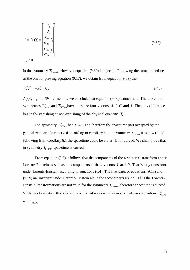
111

0

1

021

01

031

01

0 0

J

J

JJ J Q

j

J

(9.39)

in the symmetry 010203T . However equation (9.39) is rejected. Following the same procedure

as the one for proving equation (9.17), we obtain from equation (9.39) that

2 2 2

0 0 0m c J . (9.40)

Applying the SV T method, we conclude that equation (9.40) cannot hold. Therefore, the

symmetries 0

010203T and 010203T have the same four-vectors , ,J P C and j . The only difference

lies in the vanishing or non-vanishing of the physical quantity 0T .

The symmetry 0

010203T has 0 0T and therefore the spacetime part occupied by the

generalized particle is curved according to corollary 6.2. In symmetry 010203T it is

0 0T and

following from corollary 6.1 the spacetime could be either flat or curved. We shall prove that

in symmetry 010203T spacetime is curved.

From equation (3.5) it follows that the components of the 4-vector C transform under

Lorentz-Einstein as well as the components of the 4-vectors J and P . That is they transform

under Lorentz-Einstein according to equations (6.4). The first parts of equations (9.18) and

(9.19) are invariant under Lorentz-Einstein while the second parts are not. Thus the Lorentz-

Einstein transformations are not valid for the symmetry 010203T , therefore spacetime is curved.

With the observation that spacetime is curved we conclude the study of the symmetries 0

010203T

and 010203T .

112

10. THE GENERALIZED PARTICLE OF THE FIELD ,α β AND THE

CONFINEMENT EQUATION

10.1. Introduction

In this chapter we study the generalized particle of the field ,α β , for which the function

is known. This shall allow us to perform a particular application of theorem 5.1. The energy

content of the generalized particle is quantized when it is confined to a finite portion of

spacetime. We prove the condition of the confinement for the field ,α β . Following we

prove the general condition of the confinement for the field ,ξ ω .

At the end of the chapter we present a short study for the field ,α β of the symmetry

2

0221T . This study focuses on the 4-vector j of the field ,α β . That is we study the 4-vector j

in case where , ,ξ ω α β .

10.2. The Generalized Particle of the Field ,α β and the Confinement Equation

Initially we prove that the field ,α β is a special case of the field ,ξ ω . For

1

2 in equation (5.3) we obtain

, 0,1,2,32

kk k

k

bJ P k

x


, 0,1,2,32

k k

k

bck

x

and using the notation of equation (4.9) we have

0 0 1 1 2 2 3 3exp2

bz c x c x c x c x

(10.1)

From equation (10.1) and equations (5.1), (5.2) and (4.14), (4.15), we obtain

113

01

02

03

32

13

21

icz icz

z z

ξ α n

ω β τ

. (10.2)

The field ,α β is a special case of the field , ξ ω for 1

2 .

The fact that the function of the field ,α β is known allows us to derive two

impotant results about the total rest mass 0M of the generalized partcle. The first concerns

the relation between the total rest mass 0M of the generalized particle with theorem 5.2, in

case of field ,α β . From equation (10.1) we obtain

2 2 2

2 2 2 2 2 2

0 1 1 12 2 2 2

0 4

bc c c c

x c t


2 2 22 2 2 2

02 2 2 2

0 4

bM c

x c t

. (10.3)

According to equation (10.3) and theorem 5.2 the generalized photon in the field ,α β exists,

if and only if

0 0M , (10.4)

that is in the case the total rest mass of the generalized particle is zero. For 0 0M the

generalized particle appears.

Setting 1

2 in the equations of chapter 5, we arrive at the equations of the

field ,α β . For example, by setting 1

2 into equation (5.7) we obtain

114

2

2

c bzj MC

.

This is equation (4.29), as we have proved in chapter 4, for the field ,α β . On the other

hand, equation (10.3) results only because the function is known, as given by equation

(10.1) for the field ,α β .

The second conclusion concerns the consequences for the total energy 0c of the

generalized particle when it is trapped in a fixed volume V . By knowing the function we

can study the consequences for a material particle that is confined within a constant volume

V . The conserved physical quantity q , is constant within the volume V occupied by the

generalized particle. Therefore, it holds that

0

0

constant

dq icdq

dt dx

V

. (10.5)

The total conserved physical quantity q contained within the volume V occupied by

the generalized particle is

Vq dV . (10.6)

The equation (10.6) holds independently of the fact, whether the volume V of the generalized

particle variates or not. The density for the field ,α β is given by the first of the

equations (4.25)

1 01 2 02 3 032

icbzc c c . (10.7)

In the case of

1 01 2 02 3 03 0c c c ,

that is in the case of

0 n C ,

as derived from equations (3.5) and (7.24), we obtain from equation (10.7) that 0 . That

is, for the field ,α β the following equivalence holds

115

1 01 2 02 3 030 00 c c c n C . (10.8)

In the case of 0 , and from the combination of equations (10.6) and (10.7), we have

2

V

icbq zdV

n C. (10.9)

The integration in the second part of equation (10.9) is performed within the total volume V

occupied by the generalized particle. Therefore, in the case the volume V is constant, the

integral in the second part of equation (10.9) is independent of the quantiites

1 2 3, ,x x x y x z . Therefore, in the case volume V is constant, the physical quantity q in

equation (10.9) depends only on time.

Thus by combining equations (10.5) and (10.9) for a constant volume V , we obtain

0

cons t

0

tan

V

dzdV

dt

V

n C . (10.10)

Working with equation (10.10) in the general case presents some mathematical

difficulties. Therefore in the present work we will restrict our study on the simplest case. We

shall study the case for which the total momentum Cof the generalized particle is aligned on

the direction of the x - axis, that is for the case of 1 2 30, 0c c c . In this case we obtain

from equation (3.6) that 2 2 2 2

0 0 1M c c c . Furthermore it must also hold that 0 , that is

1 01 0c , according to equivalence (10.8), and since 1 0c , it must also hold that 01 0 .

Therefore our study refers to the particular case where

1

2 3

01

2 2 2 2

0 0 1

0

0

0

c

c c

M c c c

. (10.11)

We suppose that the generalized particle occupies the constant volume V defined by

the relations (10.12) in a frame of reference 1 2 3, , ,O t x x x y x z .

116

1

2 2

3 3

2 3 2 3

0

0

0

, 0, , constants

x

x L

x L

L

L L L L

. (10.12)

For the quantities , it holds that

d du c

dt dt

(10.13)

where u is the velocity with which the volume V is moving in the chosen frame of reference.

From equation (10.1), relations (10.11), and since 0x ict , we have

0 1exp exp2 2

icbc bcz t x

2 3 0 1 1

1

2exp exp exp

2 2 2V

L L icbc bc bczdV t

bc

. (10.14)

From equation (10.14) we see that equation equation (10.10) holds, if and only if

1 1

1

exp exp 02 2

exp 12

bc bc

bc

1exp 12

bc L

. (10.15)

Equation (10.15) holds only in the case the constant b of the Law of Selfvariations is an

imaginary number, b i b , b . In this case we obtain

1

1

cos 12

sin 02

,

bc L

bc L

b i b b

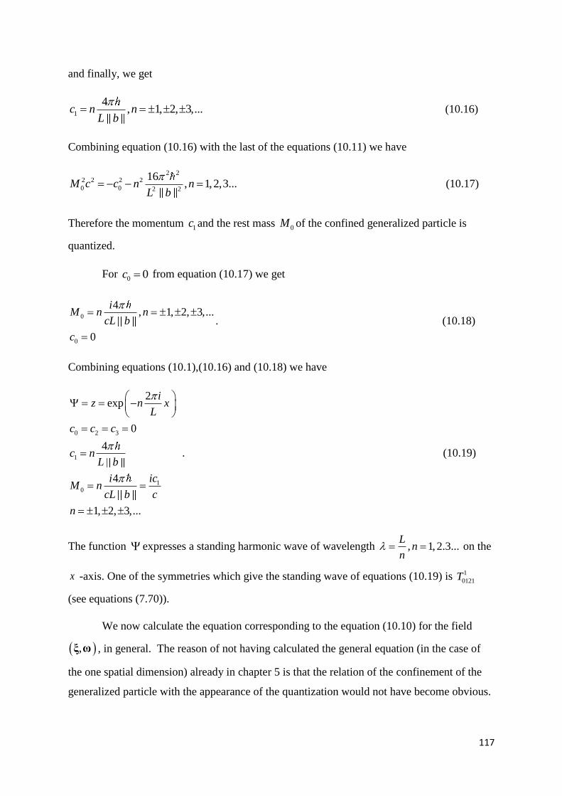
117

and finally, we get

1

4, 1, 2, 3,...c n n

L b

(10.16)

Combining equation (10.16) with the last of the equations (10.11) we have

2 22 2 2 2

0 0 2 2

16, 1,2,3...M c c n n

L b

(10.17)

Therefore the momentum 1c and the rest mass 0M of the confined generalized particle is

quantized.

For 0 0c from equation (10.17) we get

0

0

4, 1, 2, 3,...

0

iM n n

cL b

c

. (10.18)

Combining equations (10.1),(10.16) and (10.18) we have

0 2 3

1

10

2exp

0

4

4

1, 2, 3,...

iz n x

L

c c c

c nL b

iciM n

cL b c

n

. (10.19)

The function expresses a standing harmonic wave of wavelength , 1, 2.3...L

nn

on the

x -axis. One of the symmetries which give the standing wave of equations (10.19) is 1

0121T

(see equations (7.70)).

We now calculate the equation corresponding to the equation (10.10) for the field

, ξ ω , in general. The reason of not having calculated the general equation (in the case of

the one spatial dimension) already in chapter 5 is that the relation of the confinement of the

generalized particle with the appearance of the quantization would not have become obvious.

118

From equations (4.27), (4.28) and (5.7), and since it holds that 0j i c , we obtain:

01 1 02 2 03 3 01 1 02 2 03 3

icbJ J J P P P

and together with equations (5.8), (5.9) and (7.24) we have

icb

J n P n . (10.20)

From equations (10.5), (10.20) for the generalized particle occupying a constant volume V

we obtain

0

const

0

ant

V

ddV

dt

V

J n P n

J n P n . (10.21)

For 1

2 equation (10.21) gives equation (10.10), after considering equations (3.5)

and (10.1).

For the internal symmetry 0T it holds that 0M , and from equation (5.7) we

obtain 0j . Hence equation (10.5) degenerates into the identity, 0 0 , therefore the

confinement equation (10.21) does not hold. The same holds also for all the external

symmetries T zQ as follows from equation (8.4). Therefore the confinement equation

(10.21) is valid for the 44 generalized particles of the external symmetries of the sets

1 2 3 4 5, , , , of equations (7.83).

The field ,α β exists in all external symmetries, except the ones with T zQ of

the set 0 of equation (7.83). Every external symmetry of the set

1 2 3 4 5 6 expresses one of the possible states of the generalized

particle. For the field ,α β every external symmetry expresses one of the possible states of

the field. We complete the chapter with the study of the symmetry 2

0221T of the set 2 , for the

field ,α β . We consider the case where Q is electric charge, hence α is the electric field

and β the magnetic.

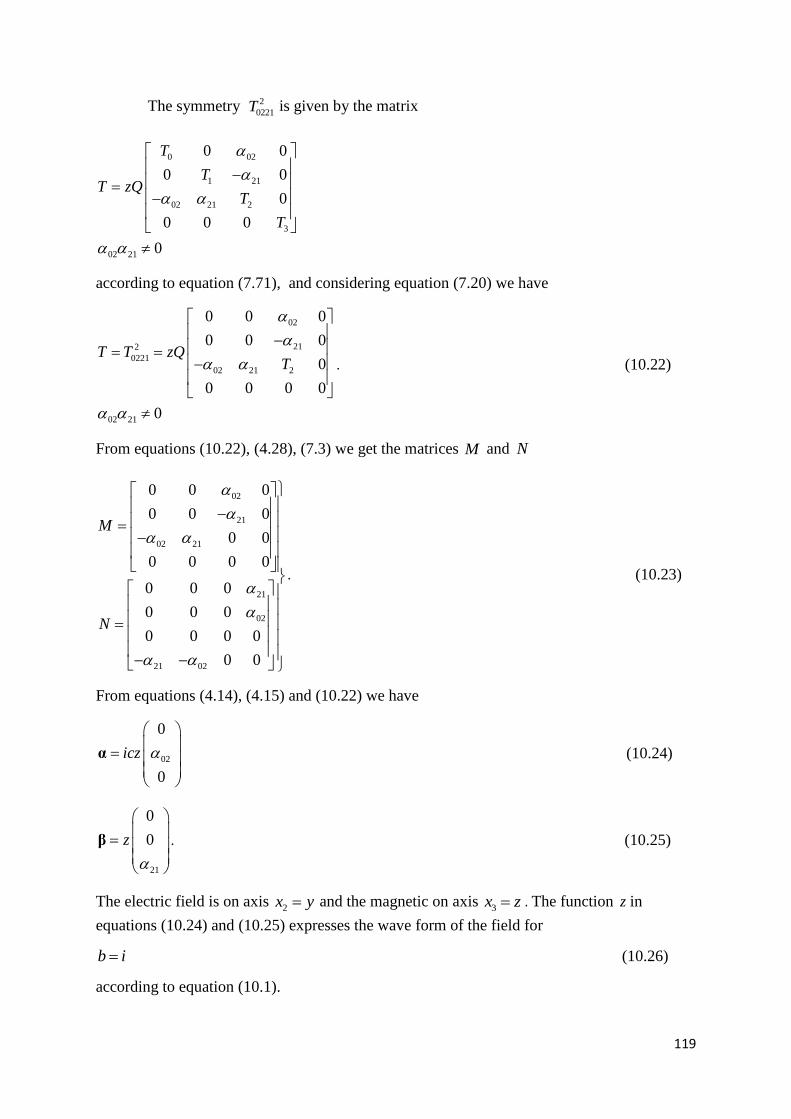
119

The symmetry 2

0221T is given by the matrix

0 02

1 21

02 21 2

3

02 21

0 0

0 0

0

0 0 0

0

T

TT zQ

T

T

according to equation (7.71), and considering equation (7.20) we have

02

212

0221

02 21 2

02 21

0 0 0

0 0 0

0

0 0 0 0

0

T T zQT

. (10.22)

From equations (10.22), (4.28), (7.3) we get the matrices M and N

02

21

02 21

21

02

21 02

0 0 0

0 0 0

0 0

0 0 0 0

0 0 0

0 0 0

0 0 0 0

0 0

M

N

. (10.23)


02

0

0

icz

α (10.24)

21

0

0z

β . (10.25)

The electric field is on axis 2x y and the magnetic on axis

3x z . The function z in

equations (10.24) and (10.25) expresses the wave form of the field for

b i (10.26)

according to equation (10.1).

120

Applying the SV M method we get the equations

2 2

02 21

21 02

0

2

0

1

0

0

0

0

0

i

iJ J Q J

Cc

P P Q C J Q

. (10.27)

The material particle exists for 0J , hence from the second of equations (10.27) we have

0 0J . (10.28)

From the fourth of equations (10.27) it follows that for 2 0c is 0C , which is impossible.

Therefore it is

2 0c . (10.29)

Considering the second of equations (10.27), the equation (10.24) can be written in the form

21

0

0

cz

α . (10.30)

From equations (10.25) and (10.30) it follows that the electric and the magnetic field have

equal norm:

α β (10.31)

From aquations (7.16), (7.17), (10.23), and taking into account the second of

equations (10.27) we have

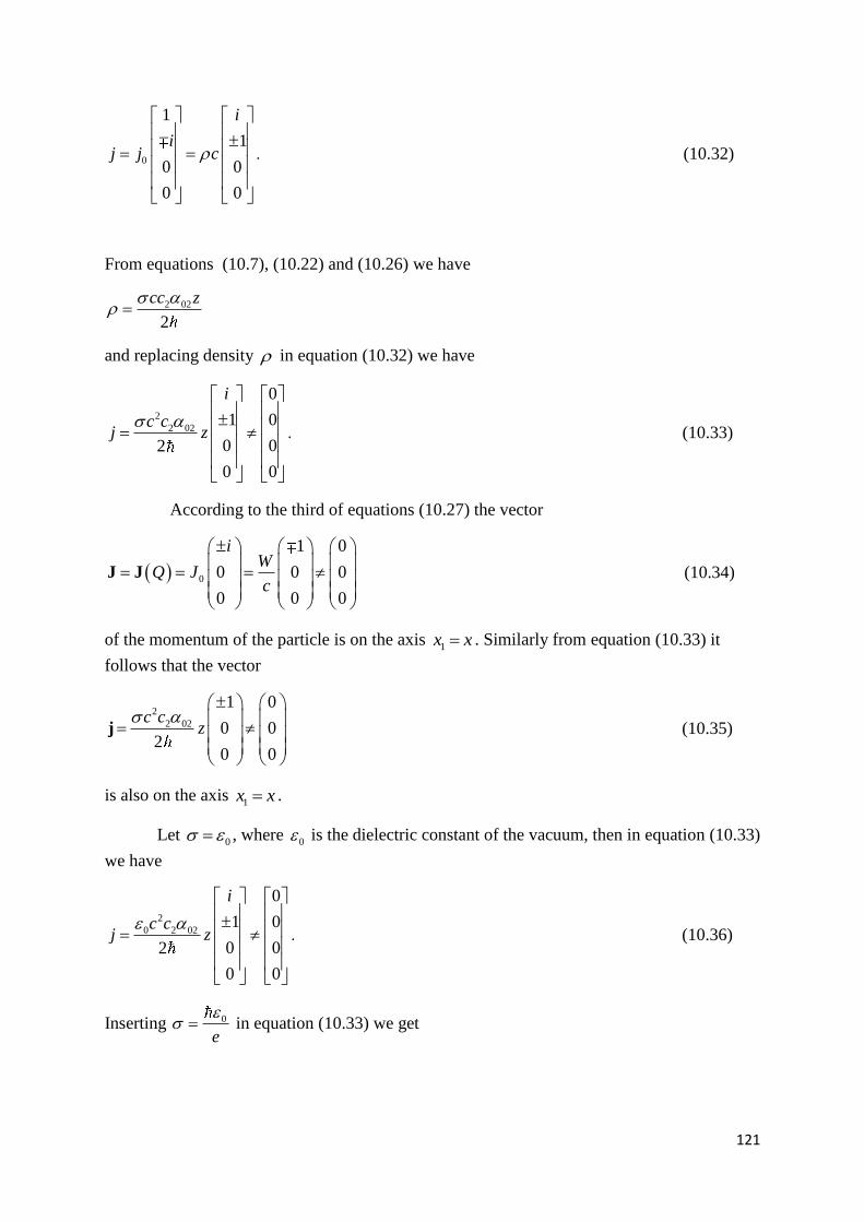
121

0

1

1

0 0

0 0

i

ij j c

. (10.32)


2 02

2

cc z

and replacing density in equation (10.32) we have

2

2 02

0

1 0

0 02

0 0

i

c cj z

. (10.33)

According to the third of equations (10.27) the vector

0

1 0

0 0 0

0 0 0

iW

Q Jc

J J (10.34)

of the momentum of the particle is on the axis 1x x . Similarly from equation (10.33) it

follows that the vector

2

2 02

1 0

0 02

0 0

c cz

j (10.35)

is also on the axis 1x x .

Let 0 , where

0 is the dielectric constant of the vacuum, then in equation (10.33)

we have

2

0 2 02

0

1 0

0 02

0 0

i

c cj z

. (10.36)

Inserting 0

e

in equation (10.33) we get

122

2

0 2 02

0

1 0

0 02

0 0

i

c cj z

e

. (10.37)

E quation (10.36) gives the 4-vector of the current density of a conserved quantity of electric

charge (see chapter 5.). Similarly equation (10.37) gives the 4-vector of the current density of

a conserved quantity of angular momentum. In both cases the vector j is on axis1x x , as

follows from equation (10.35). Finally from the third, fourth and fifth of equations (10.27)

we have

0

2 0

2

0 2 0

0

0

0

m

c M c

E cc M c

(10.38)

for the rest masses of the material particle which emerges as a consequence of the USVI.




The above eqs. completely describe the state of the field ,α β in the case of the

symmetry 2

0221T . Working in the same way we can study the field ,α β for the symmetries of

the sets 1 2 3 4 5 6, , , , , .

11. THE EXTERNAL SYMMETRY FACTOR

11.1. Introduction

In this chapter we study the factor which generates external symmetry. That is the

momentum which emerges from the USVI, which is added to the internal symmetry

momentum and eliminates the parallel property of the 4-vectors J , P and C .

In the symmetries where the field ,α β is defined the external symmetry factor is

determined by the potential of the field. The study we present demonstrates the physical

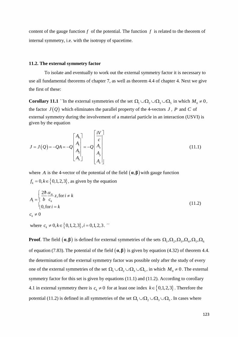
123

content of the gauge function f of the potential. The function f is related to the theorem of

internal symmetry, i.e. with the isotropy of spacetime.

11.2. The external symmetry factor

To isolate and eventually to work out the external symmetry factor it is necessary to

use all fundamental theorems of chapter 7, as well as theorem 4.4 of chapter 4. Next we give

the first of these:

Corollary 11.1 ΄΄In the external symmetries of the set 1 2 3 5 in which

0 0M ,

the factor J Q which eliminates the parallel property of the 4-vectors J , P and C of

external symmetry during the involvement of a material particle in an interaction (USVI) is

given by the equation

0

1

2

3

x

y

z

iVA

cA

AJ J Q QA Q QA

AA

A

(11.1)

where A is the 4-vector of the potential of the field ,α β with gauge function

0, 0,1,2,3kf k , as given by the equation

2, for

0, for

0

ki

ki

k

z i kb cA

i k

c

(11.2)

where 0, 0,1,2,3 , 0,1,2,3kc k i . ΄΄

Proof. The field ,α β is defined for external symmetries of the sets 1 2 3 4 5 6, , , , ,

of equation (7.83). The potential of the field ,α β is given by equation (4.32) of theorem 4.4.

the determination of the external symmetry factor was possible only after the study of every

one of the external symmetries of the set 1 2 3 5 , in which

0 0M . The external

symmetry factor for this set is given by equations (11.1) and (11.2). According to corollary

4.1 in external symmetry there is 0kc for at least one index 0,1,2,3k . Therefore the

potential (11.2) is defined in all symmetries of the set 1 2 3 5 . In cases where

124

0kc for more than one index 0,1,2,3k the potentials which emerge from equation

(11.2) are equivalent, according to equation (4.33) of theorem 4.4. The factor of external

symmetry is that what, in the field «language» we would name potential momentum of the

field ,α β of the USVI.

With the knowledge of the 4-vector J Q , as given by equations (11.1) and (11.2) we

get the 4-vector P Q of USVI from eq.

P P Q C J Q (11.3)

From equations (11.1) and (11.2) it follows that in all symmetries of the set 2 3 5

the rest mass 0m of the USVI particle is zero:

0, 0 0USVIm m (11.4)

From equations (11.3) and (11.2) it follows that the rest energy 0, 0USVIE E of the USVI

particle is not the same in every symmetry of the set 2 3 5 , in any case however we

have the equality

2

0, 0 0USVIE E M c (11.5)

where 0M the total rest mass of the generalized particle. For the

1 6N symmetries of the set

1 it can be 0, 0 0USVIm m .

In internal symmetry, i.e. the spontaneous STEM emission of the material particle

as a consequence of the Selfvariations, the 4-vectors J , P and C are parallel. When the

material particle involves in an interaction the direction of the 4-vector J Q of the potential

momentum of the USVI in spacetime depends not only on the material particle. Thus the

addition to the internal symmetry 4-vector destroys the parallel property of the 4-vectors J ,

P and C of the generalized particle. The momentum 4-vector of internal symmetry is given

by theorem 3.3, and considering equation (11.1) we have

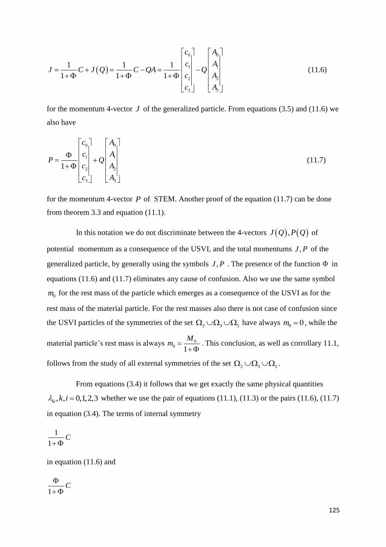
125

0 0

1 1

2 2

3 3

1 1 1

1 1 1

c A

c AJ C J Q C QA Q

c A

c A

(11.6)

for the momentum 4-vector J of the generalized particle. From equations (3.5) and (11.6) we

also have

0 0

1 1

2 2

3 3

1

c A

c AP Q

c A

c A

(11.7)

for the momentum 4-vector P of STEM. Another proof of the equation (11.7) can be done

from theorem 3.3 and equation (11.1).

In this notation we do not discriminate between the 4-vectors ,J Q P Q of

potential momentum as a consequence of the USVI, and the total momentums ,J P of the

generalized particle, by generally using the symbols ,J P . The presence of the function in

equations (11.6) and (11.7) eliminates any cause of confusion. Also we use the same symbol

0m for the rest mass of the particle which emerges as a consequence of the USVI as for the

rest mass of the material particle. For the rest masses also there is not case of confusion since

the USVI particles of the symmetries of the set 2 3 5 have always

0 0m , while the

material particle’s rest mass is always 00

1

Mm

. This conclusion, as well as corrollary 11.1,

follows from the study of all external symmetries of the set 2 3 5 .

From equations (3.4) it follows that we get exactly the same physical quantities

, , 0,1,2,3ki k i whether we use the pair of equations (11.1), (11.3) or the pairs (11.6), (11.7)

in equation (3.4). The terms of internal symmetry

1

1C

in equation (11.6) and

1C

126

in equation (11.7) do not affect the physical quantities , , 0,1,2,3ki k i . We suggest to select

one particular symmetry of the set 1 2 3 5 and do the mathematical calculations.

A good practice also for the understanding of the TSV is the proof of equations (5.10)-

(5.15), first with the pairs of 4-vectors (11.1), (11.3) and then with the pairs (11.6), (11.7).

The eqs. of the TSV are valid for the 4-vectors (11.1), (11.3) as well as for the 4-vectors

(11.6), (11.7). This fact reflects the physical content of the two symmetries, internal and

external. The spacetime isotropy implies the parallel property of the 4-vectors J and P

which in turn implies eq. 0, , 0,1,2,3ki k i , as follows from equation (3.4). The USVI

is caused by the spacetime anisotropy, which implies the relation 0ki for at least a pair of

indices , , , 0,1,2,3k i k i , as follows from equation (3.4).

We now apply corollary 11.1 to symmetry 0

010203T , whose elements we know from

chapter 9. According to equation (9.22) we have0 0c , hence from equations (11.2) we have

01

020

03

0

2 zA

bc

(11.8)


01

020

03

0

2 zQJ J Q

bc

(11.9)


0

01

020

03

0

0 2

0

0

c

zQP P Q

bc

(11.10)

for the momentum of the USVI particle.

Now from equations (11.6), (11.7), (9.22) and (11.8) we have

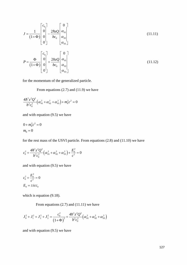
127

0

01

020

03

0

01 2

01

0

c

zQJ

bc

(11.11)

0

01

020

03

0

0 2

01

0

c

zQP

bc

(11.12)

for the momentum of the generalized particle.


2 2 2

2 2 2 2 2

01 02 03 02 2

0

40

z Qm c

b c


2 2

0

0

0 0

0

m c

m

for the rest mass of the USVI particle. From equations (2.8) and (11.10) we have

22 2 2

2 2 2 2 00 01 02 032 2 2

0

40

Ez Qc

b c c


22 00 2

0 0

0E

cc

E icc



2 2 2 22 2 2 2 2 2 200 1 2 3 01 02 032 2 2

0

4

1

c z QJ J J J

b c


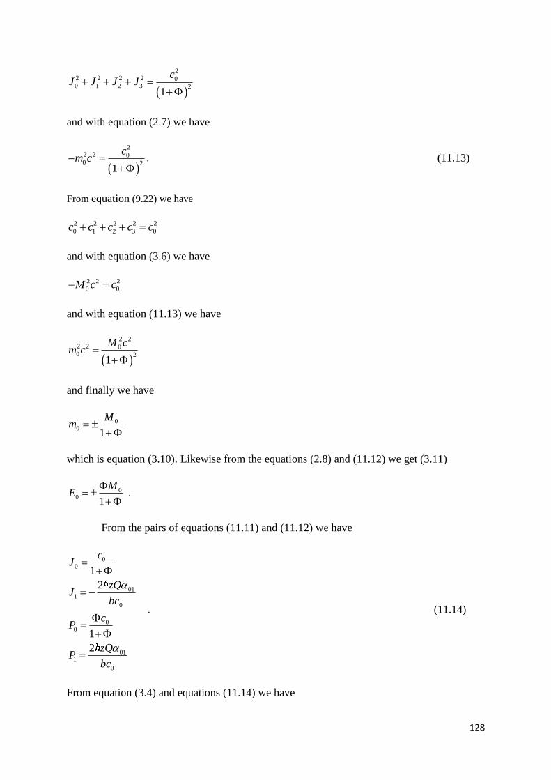
128

22 2 2 2 00 1 2 3 2

1

cJ J J J


22 2 00 2

1

cm c

. (11.13)


2 2 2 2 2

0 1 2 3 0c c c c c


2 2 2

0 0M c c


2 22 2 00 2

1

M cm c

and finally we have

00

1

Mm

which is equation (3.10). Likewise from the equations (2.8) and (11.12) we get (3.11)

00

1

ME

.

From the pairs of equations (11.11) and (11.12) we have

00

011

0

00

011

0

1

2

1

2

cJ

zQJ

bc

cP

zQP

bc

. (11.14)

From equation (3.4) and equations (11.14) we have

129

01 0 1 1 02

bJ P J P

0 01 001 01

0 0

22

2 1 1

c zQ cb zQ

bc bc

01 011 1

zQ zQ

01 01zQ . (11.15)

Equation (11.15) is the equation (4.4) for 0k and 1i . In the same way we can proof that

the pair of equations (11.1), (11.3) and (11.7), (11.8) give equations (4.4) for the symmetries

of the set 1 2 3 5 .

A question which arises from corollary 11.1 is if it can be generalized with the gauge

function , 0,1,2,3 , 0k kf k c to be different than zero ( 0kf ) in equation (4.32). The

answer is yes and is given by the following corollary:

Corollary 11.2 ΄΄For the factor J Q QA of external symmetries of the set

1 2 3 5 the 4-vector A of the potential of the field ,α β is given by eq.

2, for

, for

ki k

k i

i

k

i

fz i k

b c xA

fi k

x

(11.16)

where 0, 0,1,2,3 , 0,1,2,3kc k i and the gauge function kf satisfies the condition

, 0,1,2,3 , 0,1,2,3k kk i

i k

f fc c k i

x x

. (11.17)

In the case where 0kc for more than one index 0,1,2,3k , i.e. where

0, , , 0,1,2,3k ic c k i k i , the potentials which arise from equation (11.16) are equivalent, as

follows from equation (4.33)

2

2

4, 0, , , 0,1,2,3ki

k i k i

k i

zf f c c k i k i

b c c

(11.18)

of the theorem 4.4.΄΄

130

Proof. From equations (11.1) and (11.3) we have

, 0,1,2,3

k k

i i i

J QA

P c QA

k i

. (11.19)

Initially we ask that the combination of the equations (3.4) and (11.19) should give equation

(4.4):

2

ki k i i k

bJ P J P

2

ki k i i i k k

bzQ QA c QA QA c QA

2 2

2ki i k k i k i i k

bzQ Qc A Q A A Qc A Q A A

2

ki k i i k

bzQ Q c A c A

2ki k i i kz c A c A

b . (11.20)

Combining equations (11.20) and (11.16) for 0, 0,1,2,3 , , 0,1,2,3kc k i k i we have

2 2 ki k kki k i

k i k

f fz c z c

b b c x x

0 k kk i

i k

f fc c

x x

and finally we have

k kk i

i k

f fc c

x x

which is condition (11.17). The proof is completed by showing that the corollary is valid for

everyone of the external symmetries of the set 1 2 3 5 . The last step of the proof

is necessary because in the procedure of the proof we used equation (11.1) of corollary 11.1.

Corollary 11.1 is a special case of corollary 11.2 for 0, 0,1,2,3kf k . Via

equations (11.6), (11.7) and (11.1), (11.3) corollary 11.2 gives the 4-vectors J and P of the

material particle and the USVI particle respectively for the symmetries of the set

1 2 3 5 . It is easy to prove that the rest mass of the material particle is given by

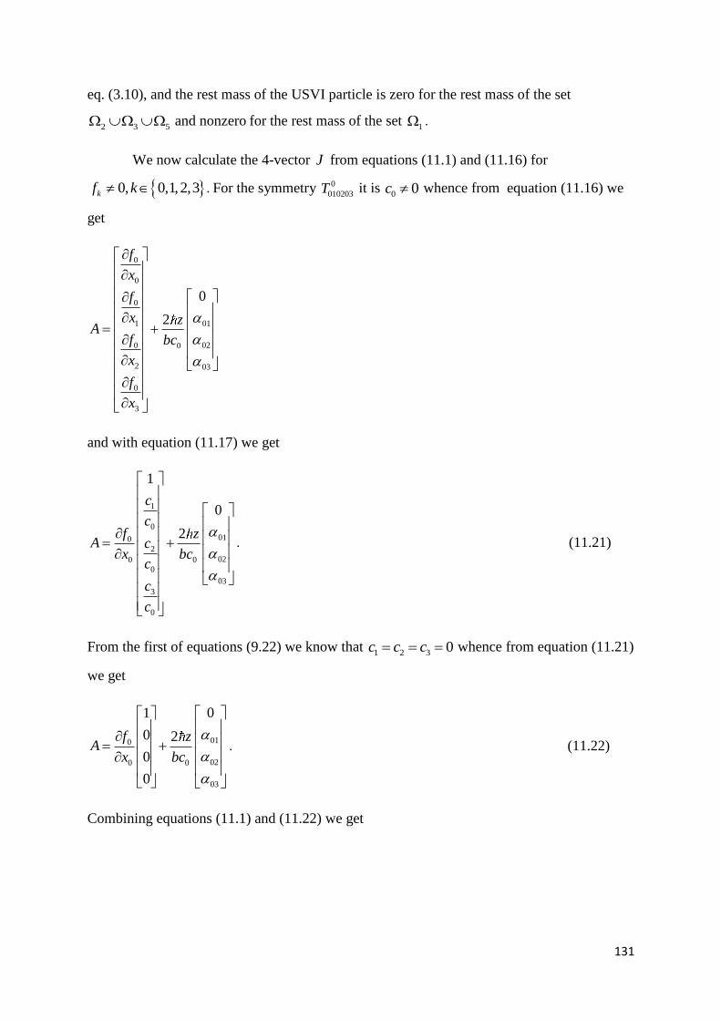
131

eq. (3.10), and the rest mass of the USVI particle is zero for the rest mass of the set

2 3 5 and nonzero for the rest mass of the set 1 .

We now calculate the 4-vector J from equations (11.1) and (11.16) for

0, 0,1,2,3kf k . For the symmetry 0

010203T it is 0 0c whence from equation (11.16) we

get

0

0

0

1 01

020 0

2 03

0

3

0

2

f

x

f

x zA

f bc

x

f

x


1

0

010

2

020 0

0

03

3

0

1

0

2

c

cf z

A cx bc

c

c

c

. (11.21)

From the first of equations (9.22) we know that 1 2 3 0c c c whence from equation (11.21)

we get

010

020 0

03

01

0 2

0

0

f zA

x bc

. (11.22)

Combining equations (11.1) and (11.22) we get

132

010

020 0

03

01

0 2

0

0

f zQJ Q

x bc

. (11.23)

Comparing equations (11.11) and (11.23) se see that the procedure of proof we followed

gives us equation (11.11) for 0 0f . Moreover a valid eq. is

0 0

0

0

1 2 3

1

0

0

f cQ

x

c

c c c

. (11.24)

Equation (11.24) gives the relation of the gauge function 0f with the function and the

charge Q for symmetry 0

010203T . An analogous equation is valid for every external symmetry

with determined field ,α β , that is for the set 1 2 3 4 5 6 . The

comparison of equations (11.11) and (11.23) reveals the physical content of the gauge

function f in the context of the TSV. The gauge function f is related with internal

symmetry, i.e. with isotropic emission of the STEM from material particles.

The method we presented results in equation (11.11) in a different way than from

the SV M method. The SV M method as well as the above proof procedure may be

applied for the external symmetries where the field ,α β , is determined i.e. for the set

1 2 3 4 5 6 .

For the symmetries T zQ of the set 0 the field ,α β is not defined. Therefore

the present study does not concern the symmetries T zQ . The cause of external

symmetries for the symmetries of the set 0 is given by corollary 8.1 of chapter 8.

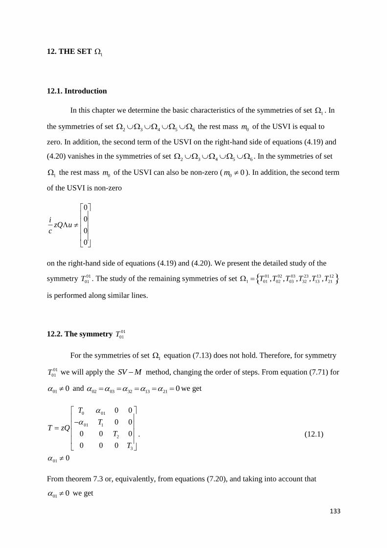
133

12. THE SET 1

12.1. Introduction

In this chapter we determine the basic characteristics of the symmetries of set 1 . In

the symmetries of set 2 3 4 5 6 the rest mass

0m of the USVI is equal to

zero. In addition, the second term of the USVI on the right-hand side of equations (4.19) and

(4.20) vanishes in the symmetries of set 2 3 4 5 6 . In the symmetries of set

1 the rest mass 0m of the USVI can also be non-zero (

0 0m ). In addition, the second term

of the USVI is non-zero

0

0

0

0

izQ u

c

on the right-hand side of equations (4.19) and (4.20). We present the detailed study of the

symmetry 01

01T . The study of the remaining symmetries of set 01 02 03 23 13 12

1 01 02 03 32 13 21, , , , ,T T T T T T

is performed along similar lines.

12.2. The symmetry 01

01T

For the symmetries of set 1 equation (7.13) does not hold. Therefore, for symmetry

01

01T we will apply the SV M method, changing the order of steps. From equation (7.71) for

01 0 and 02 03 32 13 21 0 we get

0 01

01 1

2

3

01

0 0

0 0

0 0 0

0 0 0

0

T

TT zQ

T

T

. (12.1)

From theorem 7.3 or, equivalently, from equations (7.20), and taking into account that

01 0 we get

134

2 3 0T T (12.2)

therefore, equation (12.1) becomes

0 01

01 1

01

0 0

0 0

0 0 0 0

0 0 0 0

0

T

TT zQ

. (12.3)

From the second of equations (4.6) for , , 0,1,2 , 0,1,3 , 0,2,3 , 1,2,3i k we

get

0 12 2 01 1 20

0 13 3 01 1 30

0 23 3 02 2 30

1 23 3 12 2 31

0

0

0

0

J a J a J a

J a J a J a

J a J a J a

J a J a J a

and taking into account that , , , 0,1,2,3ki ik k i k i , and the elements of matrix T as

given by equation (12.3) we get

2 01

3 01

0

0

J

J

and since 01 0 we get

2 3 0J J (12.4)

0

1

0

0

J

JJ

. (12.5)

Equation (12.5) gives the four-vector J Q . As we have already mentioned, we will use the

symbol J in equation (11.1) as well as in equation (11.6), since there is no issue of confusion

between the four-vectors J and J Q .

From equations (2.13) and (12.3), (12.5), and considering that 0zQ we get

135

0 01 0

01 1 1

0 0 0

0 0 0

0 0 0 0 0 0

0 0 0 0 0 0

T a J

a T J

and therefore

0 0 01 1

01 0 1 1

0

0

T J J

J T J

. (12.6)

Equations (12.6) constitute a 2 2 homogeneous system with the momenta 0J and

1J as

unknowns. Since it is 2 3 0J J and 0J system (12.6) has a non-zero solution and ,

therefore, its determinant is equal to zero, that is

2

0 1 01 0T T . (12.7)

From equation (12.7) and because 01 0 we get

0 1 0T T . (12.8)

Thus, from equation (12.3) and relation (12.8) we get

0 01

01 101

01

0 0

0 0

0 0 0 0

0 0 0 0

T

TT zQ

. (12.9)

We reitterate that, according to our naming convention, the elements in the matrices of the

sets of equation (7.83) are non-zero.

From the first of equations (4.6) for , , 0,1,2 , 0,1,3 , 0,2,3 , 1,2,3i k we get

0 12 2 01 1 20

0 13 3 01 1 30

0 23 3 02 2 30

1 23 3 12 2 31

0

0

0

0

c a c a c a

c a c a c a

c a c a c a

c a c a c a

and taking into account that , , , 0,1,2,3ki ik k i k i , and the elements of matrix 01

01T as

given by equation (12.9) we get

136

2 01

3 01

0

0

c

c


2 3 0c c (12.10)

0

1

0

0

c

cC

. (12.11)

From equations (3.4) and (4.4) we get

01 1 0 0 12

bzQ c J c J . (12.12)

Given that 01 0 we get from equation (12.12) relation

0 1 1 0c J c J . (12.13)

From relation (12.13) it follows that the four-vectors J and C of equations (12.5) and

(12.11) are not parallel.

Applying the SV T method it is easy to determine that equation (12.12) is

compatible with the symmetry 01

01T only when 0 10 0c c or

0 10 0c c . Therefore,

the four-vector C is expressed in the following two ways

0

0

0

0

0

0

c

C

c

(12.14)

1

1

0

0

0

0

cC

c

. (12.15)

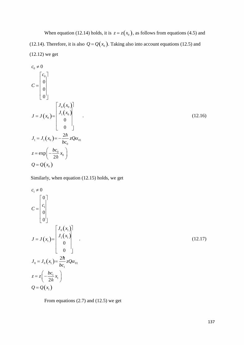
137

When equation (12.14) holds, it is 0z z x , as follows from equations (4.5) and

(12.14). Therefore, it is also 0Q Q x . Taking also into account equations (12.5) and

(12.12) we get

0

0

0 0

1 0

0

1 1 0 01

0

00

0

0

0

0

0

0

0

2

exp2

c

c

C

J x

J xJ J x

J J x zQbc

bcz x

Q Q x

. (12.16)

Similarly, when equation (12.15) holds, we get

1

1

0 1

1 1

1

0 0 1 01

1

11

1

0

0

0

0

0

0

2

2

c

cC

J x

J xJ J x

J J x zQbc

bcz z x

Q Q x

. (12.17)


138

2 2 2 2

0 1 0 0J J m c . (12.18)

We now prove that the rest mass 0m of the USVI particle can be non-zero in the symmetry

01

01T , that is

0 0m . (12.19)

For 0 0m in equation (12.18) we apply the SV T method differentiating with respect to

, 0,1,2,3x , and considering equations (2.10), (4.4) and (2.6) we get

20 010 1 0 0

J mJJ J m c

x x x

2

0 0 0 1 1 1 0 0 0b b b

J P J zQ J P J zQ m c P m

2 2 2 2

0 1 0 0 0 1 1 0b

P J J m c zQ J J


0 0 1 1 0zQ J J

and because 0zQ we have

0 0 1 1 0J J . (12.20)

For succesive 0,1,2,3 in equation (12.20) we get:

For 0 , 0 0 1 01 0J T J which is the first of equations (12.6).

For 1 , 0 10 1 1 0J J T and equivalently

0 01 1 1 0J J T which is the second of

equations (12.6).

For 2 , 0 20 1 21 0J J which holds since

20 21 0 for symmetry 01

01T .

For 3 , 0 30 1 31 0J J which holds since

30 21 0 for symmetry 01

01T .

We prove the equivalence

0 1 00m T T (12.21)

139

for symmetry 01

01T .

Proof. We prove that it is impossible to have

0 1 00m T T . (12.22)

For 1 0T T from equation (7.76) of theorem 7.6 we have

2 2 2

0 0 1 0T J J


2 2 2

0 0 0T m c

and from the relation (12.8) we get 0 0m which is absurd since we have assumed that

0 0m . Therefore we have the equivalence (12.21).

We prove now that for 0 0m the physical quantities

0T and 1T are not constant and

are given by the equations

0 1

0

22 01

0

0 00

2

011

0

0 0

0 0

0

ex

,

p 1

c c

m

Tbc x

co s

T

n a t

T

t n

(12.23)

0 1

0

22 01

1

1 11

2

010

1

1 1

0 0

0

ex

,

p 1

c c

m

Tbc x

co s

T

n a t

T

t n

. (12.24)

140

Proof. We prove the equation (12.23) and similarly equation (12.24) is proved. For

0 10 0c c from equations (3.4) and (4.4) we have

01 1 0 0 1

01 0 1

2

02

bzQ c J c J

bzQ c J

011

0

2J zQ

bc

. (12.25)

Form equation (12.25) and the first of equations (12.6) we have

0 0 01 1

010 1

0

0T J J

J JT

2

010 0 0

0 0

2 zQJ J x

bc T

. (12.26)

Differentiating equation (12.26) with respect to 0x we get

2 2

0 01 0 01

2

0 0 0 0 0 0 0

2 2 1 d zQdJ dTzQ

dx bc T dx bc T dx

and with equations (2.6), (2.10), (4.4) and (4.9) for 0 1 2 30 0c c c c we have

2 2

01 0 01 00 0 0 2

0 0 0 0 0

2 2 1

2

dT bcb zQ bP J zQT zQ

bc T dx bc T


2 2

01 0 010 2

0 0 0 0

2 dT zQzQzQT

bc T dx T

and because of 0zQ we have

23 201 0

0 01 0

0 0

2 dTT T

bc dx

and solving the differential equation we get

141

2

0

00 0

1

exp 1

Tbc

x

and with equation (12.7) we get equation (12.23).

Consequently, the rest mass 0m of the USVI particle can be non-zero in the symmetry 01

01T .

We now check whether it can be 0 0m in equation (12.18). For

0 0m we get

2 2

0 1 0J J

1 0J iJ . (12.27)

We apply the SV T method, we deferentiate equation (12.27) with respect to

, 0,1,2,3x , and, taking into account equations (2.10) and (4.4) we get

01JJ

ix x

1 1 0 0

b bP J zQ i P J zQ


1 0zQ izQ


1 0i . (12.28)

For succesive 0,1,2,3 in equation (12.14) we get:

For 0 , 01 00 0i iT and equivalently

0 01T i . (12.29)

For 1 , 1 10T i and equivalently

1 01T i . (12.30)

For 2 , 21 20i which holds since

20 21 0 for the symmetry 01

01T .

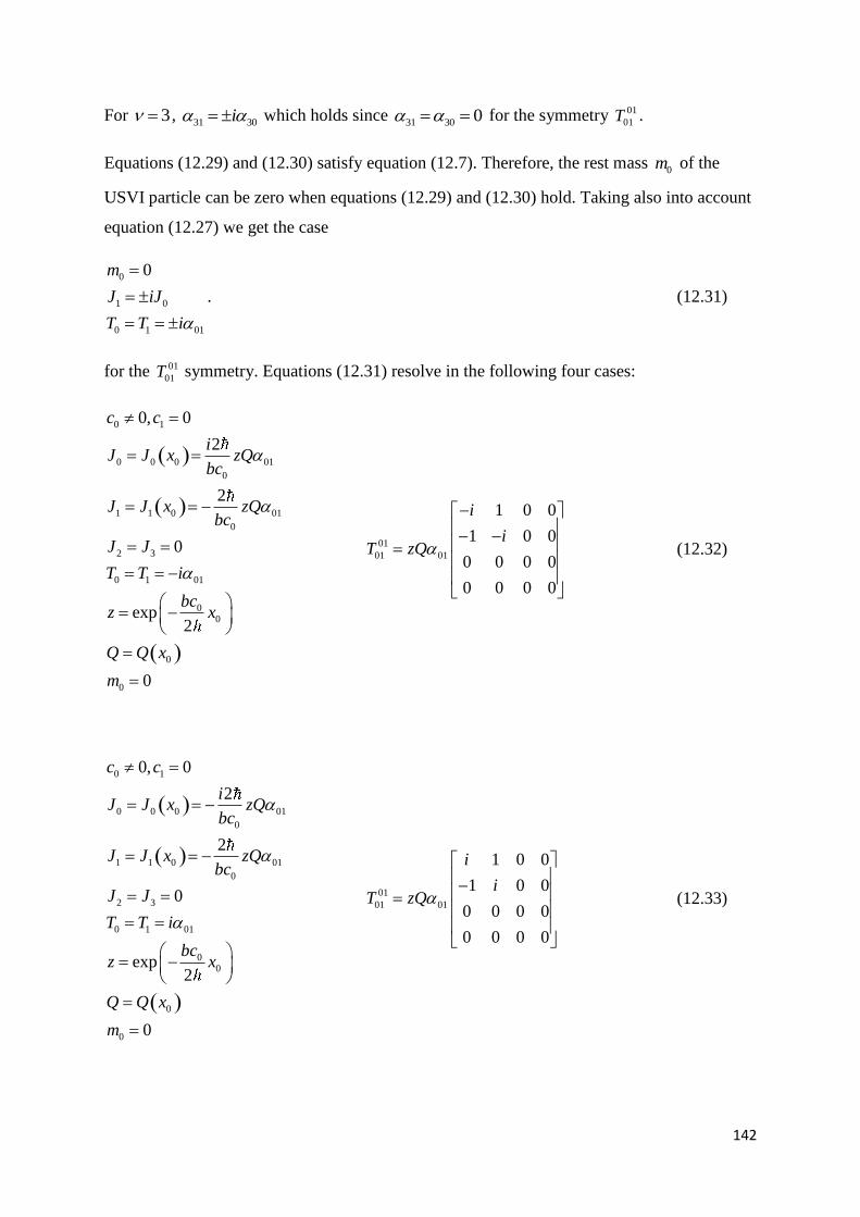
142

For 3 , 31 30i which holds since

31 30 0 for the symmetry 01

01T .

Equations (12.29) and (12.30) satisfy equation (12.7). Therefore, the rest mass 0m of the

USVI particle can be zero when equations (12.29) and (12.30) hold. Taking also into account

equation (12.27) we get the case

0

1 0

0 1 01

0m

J iJ

T T i

. (12.31)

for the 01

01T symmetry. Equations (12.31) resolve in the following four cases:

0 1

0 0 0 01

0

1 1 0 01

0

2 3

0 1 01

00

0

0

0, 0

2

2

0

exp2

0

c c

iJ J x zQ

bc

J J x zQbc

J J

T T i

bcz x

Q Q x

m

01

01 01

1 0 0

1 0 0

0 0 0 0

0 0 0 0

i

iT zQ

(12.32)

0 1

0 0 0 01

0

1 1 0 01

0

2 3

0 1 01

00

0

0

0, 0

2

2

0

exp2

0

c c

iJ J x zQ

bc

J J x zQbc

J J

T T i

bcz x

Q Q x

m

01

01 01

1 0 0

1 0 0

0 0 0 0

0 0 0 0

i

iT zQ

(12.33)

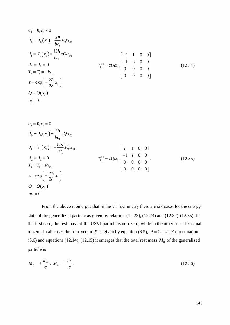
143

0 1

0 0 1 01

1

1 1 1 01

1

2 3

0 1 01

11

1

0

0, 0

2

2

0

exp2

0

c c

J J x zQbc

iJ J x zQ

bc

J J

T T i

bcz x

Q Q x

m

01

01 01

1 0 0

1 0 0

0 0 0 0

0 0 0 0

i

iT zQ

(12.34)

0 1

0 0 1 01

1

1 1 1 01

1

2 3

0 1 01

11

1

0

0, 0

2

2

0

exp2

0

c c

J J x zQbc

iJ J x zQ

bc

J J

T T i

bcz x

Q Q x

m

01

01 01

1 0 0

1 0 0

0 0 0 0

0 0 0 0

i

iT zQ

. (12.35)

From the above it emerges that in the 01

01T symmetry there are six cases for the energy

state of the generalized particle as given by relations (12.23), (12.24) and (12.32)-(12.35). In

the first case, the rest mass of the USVI particle is non-zero, while in the other four it is equal

to zero. In all cases the four-vector P is given by equation (3.5), P C J . From equation

(3.6) and equations (12.14), (12.15) it emerges that the total rest mass 0M of the generalized

particle is

0 10 0

ic icM M

c c . (12.36)

144




From equation (7.3), and taking into account the elements of matrix 01

01T , we get

01

01

0 0 0 0

0 0 0 0

0 0 0

0 0 0

N

and from equation (7.17) we get

0

1

01 2

01 3

0 0 0 0 0

0 0 0 0 0

0 0 0 0

0 0 0 0

j

j

j

j

and, equivalently,

01 3

01 2

0

0

j

j


2 3 0j j (12.37)

0

1

0

0

j

jj

(12.38)

for the current density four-vector j of the conserved physical quantities in the 01

01T

symmetry.

We obtain a different expression of the four-vector j from equation (5.7). From

equation (4.28) we get

145

01

01

0 0 0

0 0 0

0 0 0 0

0 0 0 0

M

(12.39)

for symmetry 01

01T . Combining equations (5.7) and (3.5) we get

2

2

c bj M J C

c bj MJ MC

and with equations (12.39) and (12.5), (12.14), (12.15) we get

1

20 001

0

0 0

0 0

J

J cc bj

(12.40)

1 1

2001

0

0 0

0 0

J c

Jc bj

(12.41)

where , the degrees of freedom of the TSV.

For the field ,α β it is 1

2 and z and, substituting in equations (12.40)

and (12.41), we get

2

0010

0

0

02

0

0

cc b zj j x

c

(12.42)

146

1

2

011

1

0

02

0

0

c

c b zj j x

c

. (12.43)

Using succesive ( , ) 0,1 , 0,2 , 0,3 , 3,2 , 1,3 , 2,1k i in equation (5.17) we get

22 2 01

01 2

0 0 1

0

2

0

3

1

3

1

2

0

0

0

0

jjc

x x x

j

x

j

x

j

x

j

x

and taking also into account equation (12.38) we get

22 2 01

01 2

0 0 1

0 0 0 1

1 1 0 1

2 3

,

,

0

jjc

x x x

j j x x

j j x x

j j

. (12.44)

Equations (12.44) give the wave-equation of the TSV for the 01

01T symmetry.

In the case of the ,α β field, we know the four-vector j in every symmetry of the set

1 2 3 4 5 6 . For the 01

01T symmetry, the four-vector j of field ,α β is

given by equations (12.42) and (12.43). Equations (12.44) concern the case of equations

(12.40) and (12.41).

From equations (4.19), (12.38) and taking into account the elements of matrix 01

01T we

obtain the USVI of the 01

01T symmetry:

147

0 0 0 1

01

1 1 1 10 0

2 3 0

J J T ic ud dQ i izQ zQ

J J Tu icdx Qdx c c

J J

. (12.45)

We note that the term

0 0

1 1

T uizQ

Tuc

on the right-hand side of equation (12.45) is different than zero, as follows from equation

(12.8). The fact that this term is not zero in the USVI is a common characteristic of the

symmetries of set 1 .

In the preceeding study we denoted J the four-vector J Q . Knowing the four-

vector J Q we can calculate the four-vectors J and P from equations (7.86). The

calculation of the four-vectors J and P can also be performed through equations (11.6) and

(11.7). The potential A is given by equation (11.16) for 0 1 2 30 0c c c c and

1 0 2 30 0c c c c , as emerges from equations (12.14), (12.15).

13. THE SET 4

13.1. Introduction

In this chapter we determine the basic characteristics of set 4 . We present the

analytical study of the 01033221T symmetry. The rest of the symmetries of set

4 01023213 01033221 02031321, ,T T T can be studied in a similar way.

In the symmetries of set 4 the rest masses

0m , 0

2

E

c and

0M are equal to zero,

00 02

0E

m Mc

. The same is true for the four-vector j of the density of the conserved

quantities of the generalized particle, which is 0j . Additionally, the generalized particle is

148

always in the form of the generalized photon. These three characteristics are also shared by

the 010203321321T symmetry of set

6 .

13.2. The symmetry 01033221T

The symmetry 01033221T is given by equation (7.71) when

01 03 32 21 0 and

02 13 0

0 01 03

01 1 21

21 2 32

03 32 3

01 03 32 21

0

0

0

0

0

T

TT zQ

T

T

. (13.1)

From theorem 7.3 or, equivalently, from equations (7.20) we get 0 1 2 3 0T T T T

therefore, from equation (13.1) we get

03

01

01 03 21

0101 21

01033221 01

21 32 3221

01 0103 32

03 32

01 01

0 1 0

0 01 0 0

0 0

0 00 0

0 0

0 0

T zQ zQ

. (13.2)

We reiterate that, according to the notation we use, the elements in the matrices of equation

(7.83) have non-zero values.

From equations (7.2) and taking into account the elements of matrix 01033221T we get,

after the calculations, equations

01 032 0 0

21 32

01 213 1 1

03 32

J J J

J J J

. (13.3)

From equations (13.3) we get

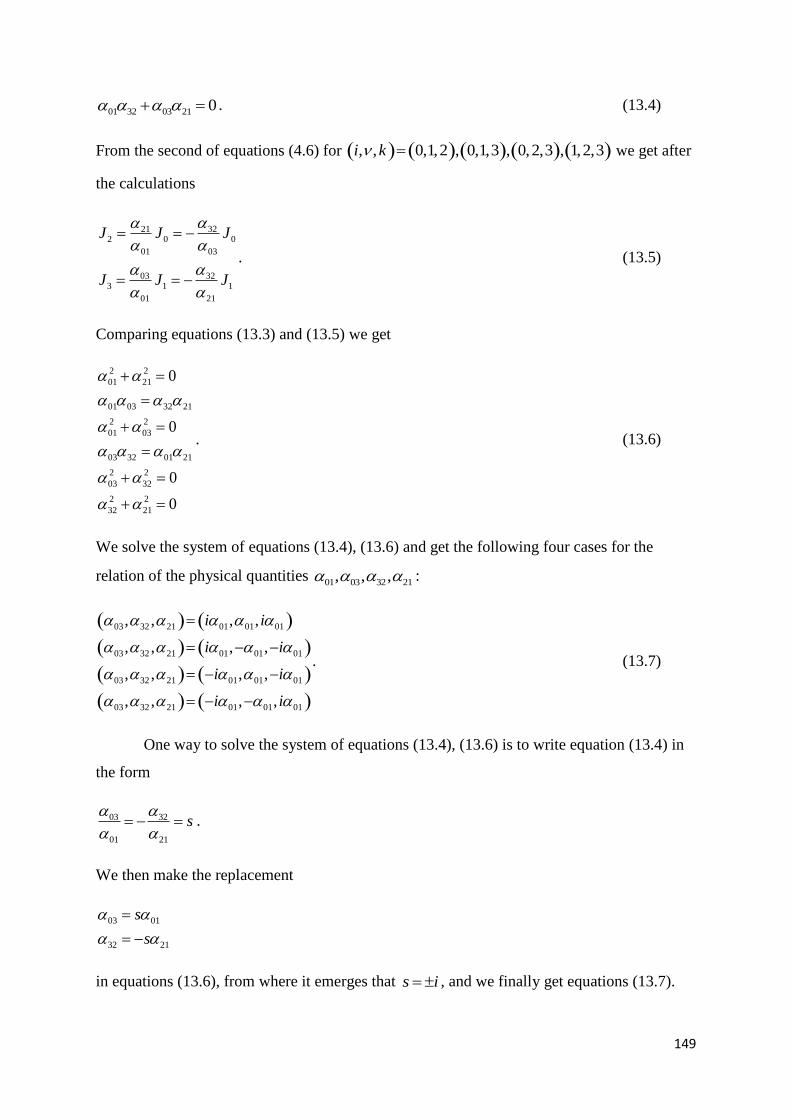
149

01 32 03 21 0 . (13.4)

From the second of equations (4.6) for , , 0,1,2 , 0,1,3 , 0,2,3 , 1,2,3i k we get after

the calculations

32212 0 0

01 03

03 323 1 1

01 21

J J J

J J J

. (13.5)

Comparing equations (13.3) and (13.5) we get

2 2

01 21

01 03 32 21

2 2

01 03

03 32 01 21

2 2

03 32

2 2

32 21

0

0

0

0

. (13.6)

We solve the system of equations (13.4), (13.6) and get the following four cases for the

relation of the physical quantities 01 03 32 21, , , :

03 32 21 01 01 01

03 32 21 01 01 01

03 32 21 01 01 01

03 32 21 01 01 01

, , , ,

, , , ,

, , , ,

, , , ,

i i

i i

i i

i i

. (13.7)

One way to solve the system of equations (13.4), (13.6) is to write equation (13.4) in

the form

03 32

01 21

s

.

We then make the replacement

03 01

32 21

s

s

in equations (13.6), from where it emerges that s i , and we finally get equations (13.7).

150


0

1

210

01

031

01

J

J

JJ

J

. (13.8)


after the calculations

0

1

210

01

031

01

c

c

cC

c

. (13.9)

In the symmetry 01033221T it is

01 0 , therefore, from equation (3.4) we get

01 1 0 0 1 02

bc J c J

0 1 1 0c J c J . (13.10)

Because of relation (13.10) the four-vectors J and C , as given by equations (13.8) and

(13.9) cannot be parallel.

From equations (13.8), (13.9) and (3.5) we get

0 0

1 1

210 0

01

031 1

01

c J

c J

c JP

c J

. (13.11)


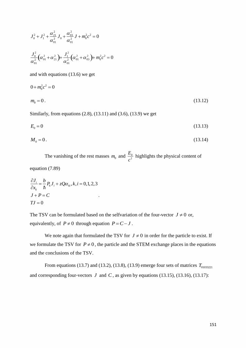
151

222 2 2 203210 1 0 02 2

01 01

0J J J J m c

2 2

2 2 2 2 2 20 101 21 01 03 02 2

01 01

0J J

m c


2 2

00 0m c

0 0m . (13.12)

Similarly, from equations (2.8), (13.11) and (3.6), (13.9) we get

0 0E (13.13)

0 0M . (13.14)

The vanishing of the rest masses 0m and 0

2

E

c highlights the physical content of

equation (7.89)

, , 0,1,2,3

0

ik i ki

k

J bP J zQ k i

x

J P C

TJ

.

The TSV can be formulated based on the selfvariation of the four-vector 0J or,

equivalently, of 0P through equation P C J .




From equations (13.7) and (13.2), (13.8), (13.9) emerge four sets of matrices 01033221T

and corresponding four-vectors J and C , as given by equations (13.15), (13.16), (13.17):

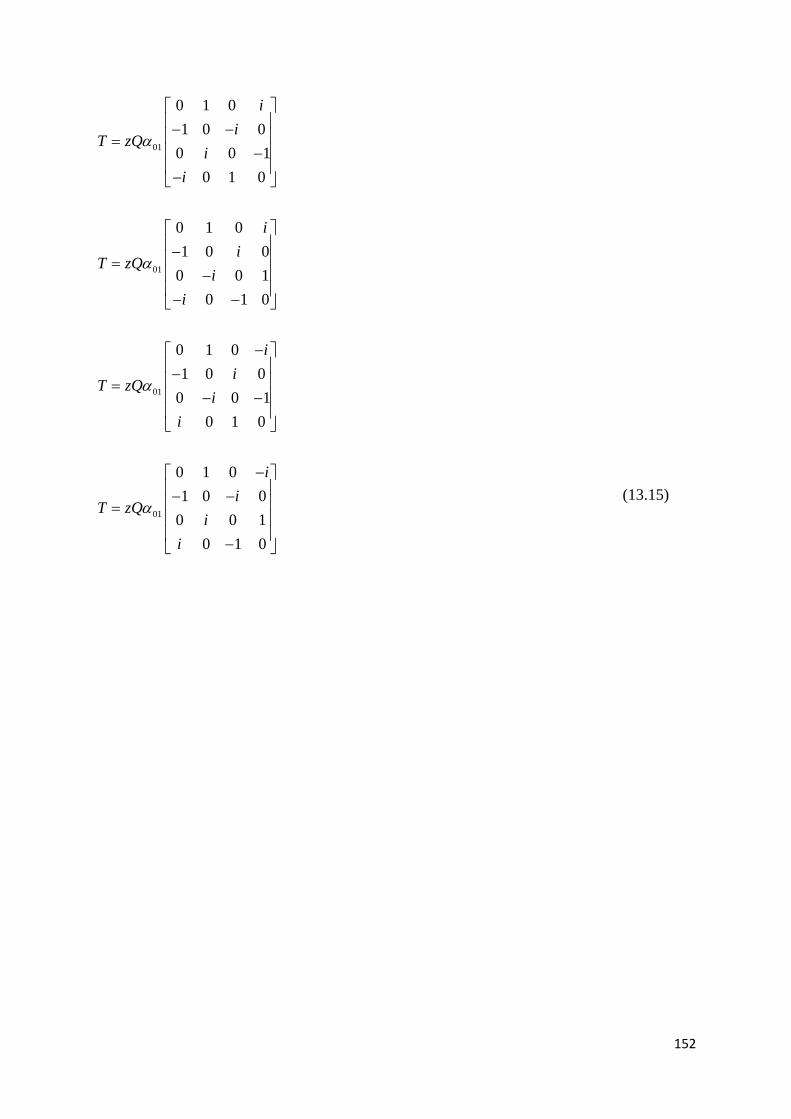
152

01

01

01

01

0 1 0

1 0 0

0 0 1

0 1 0

0 1 0

1 0 0

0 0 1

0 1 0

0 1 0

1 0 0

0 0 1

0 1 0

0 1 0

1 0 0

0 0 1

0 1 0

i

iT zQ

i

i

i

iT zQ

i

i

i

iT zQ

i

i

i

iT zQ

i

i

(13.15)

153

0

1

0

1

0

1

0

1

0

1

0

1

0

1

0

1

J

JJ

iJ

iJ

J

JJ

iJ

iJ

J

JJ

iJ

iJ

J

JJ

iJ

iJ

(13.16)

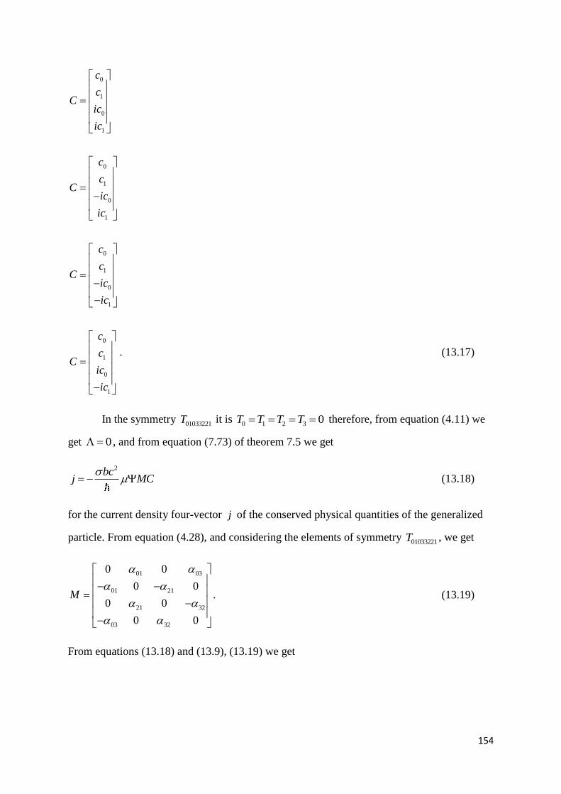
154

0

1

0

1

0

1

0

1

0

1

0

1

0

1

0

1

c

cC

ic

ic

c

cC

ic

ic

c

cC

ic

ic

c

cC

ic

ic

. (13.17)


0 1 2 3 0T T T T therefore, from equation (4.11) we

get 0 , and from equation (7.73) of theorem 7.5 we get

2bcj MC

(13.18)

for the current density four-vector j of the conserved physical quantities of the generalized

particle. From equation (4.28), and considering the elements of symmetry 01033221T , we get

01 03

01 21

21 32

03 32

0 0

0 0

0 0

0 0

M

. (13.19)

From equations (13.18) and (13.9), (13.19) we get

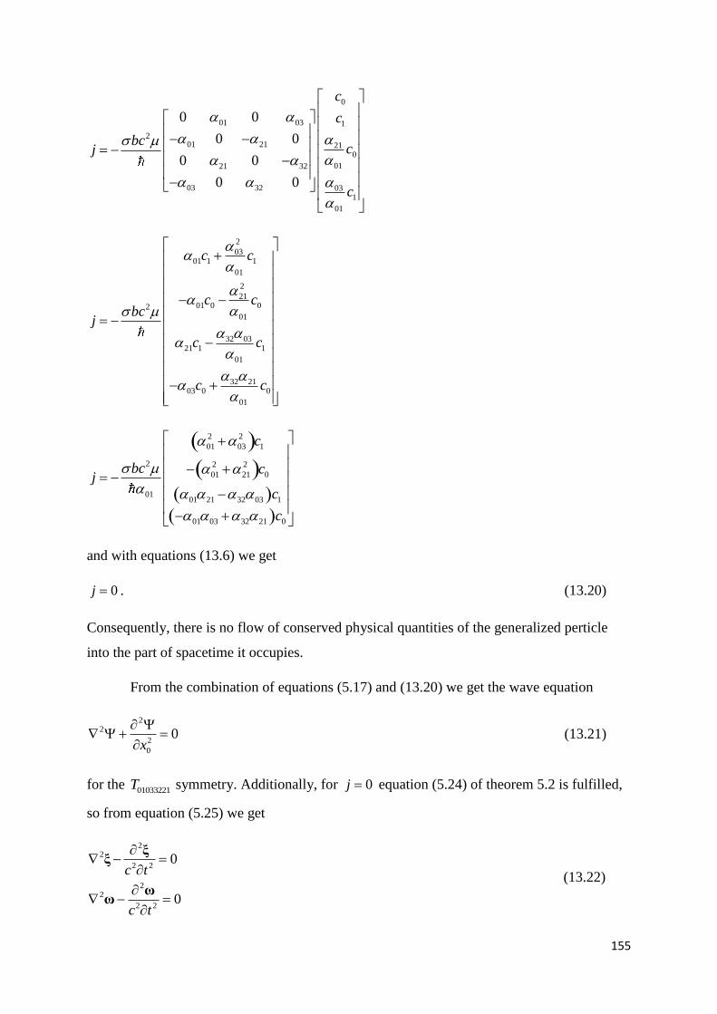
155

0

01 03 1

201 21 21

0

0121 32

03 32 031

01

0 0

0 0

0 0

0 0

c

c

bccj

c

2

0301 1 1

01

2

2101 0 02

01

32 0321 1 1

01

32 2103 0 0

01

c c

c cbc

j

c c

c c

2 2

01 03 1

2 2 2

01 21 0

0101 21 32 03 1

01 03 32 21 0

c

bc cj

c

c


0j . (13.20)

Consequently, there is no flow of conserved physical quantities of the generalized perticle

into the part of spacetime it occupies.

From the combination of equations (5.17) and (13.20) we get the wave equation

22

2

0

0x

(13.21)

for the 01033221T symmetry. Additionally, for 0j equation (5.24) of theorem 5.2 is fulfilled,

so from equation (5.25) we get

22

2 2

22

2 2

0

0

c t

c t

ξξ

ωω

(13.22)

156

for the field ,ξ ω . Consequently, in the symmetries of set 4 , the generalized particle is

always in the form of the generalized photon.

In the preceeding study we denoted J the four-vector J Q . Knowing the four-

vector J Q we can calculate the four-vectors J and P from equations (7.86). The 01033221T

symmetry has four versions as defined by equations (13.7). Consequently, from the

cobination of equations (7.86) and (13.7) four versions of the four-vectors J and P emerge.

The four-vectors J and P can also be calculated through equations (11.6), (11.7) and

(11.16). We note that in the 01033221T symmetry, equation (11.18) is applied since it can be

0 1 0c c .

Similarly, for every case of equations (13.7) we can calculate the USVI from

equations (4.19) and (4.20). We note that the term

izQ u

c

of the USVI vanishes

0

0

0

0

izQ u

c

since in the 01033221T symmetry it is 0 .

14. THE EMPTY SET 5 AND THE DIMENSIONALITY OF SPACETIME

14.1. Introduction

In this chapter we prove that 5 is the empty set,

5 . We come to this

conclusion by applying the SV T method. We present the detailed study for the 0103321321T

symmetry. The proof for the remaining symmetries of set

5 0102033213 0102033221 0102023213 0102321321 0103321321 0203321321, , , , ,T T T T T T is similar.

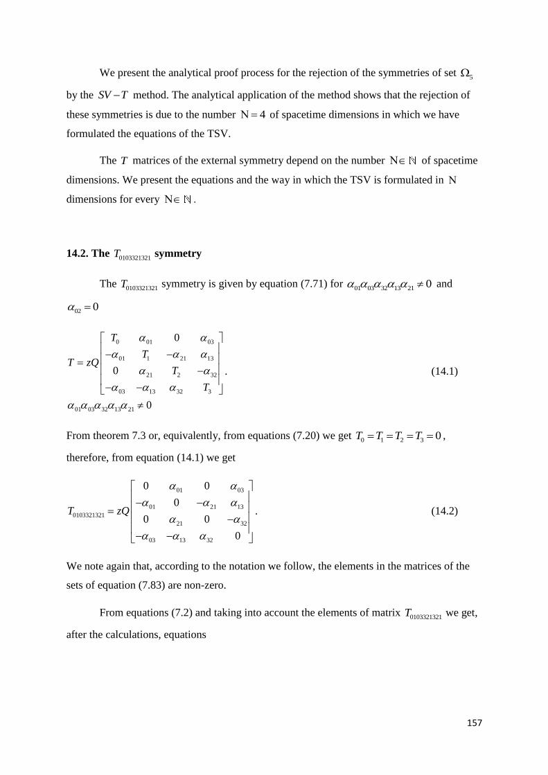
157

We present the analytical proof process for the rejection of the symmetries of set 5

by the SV T method. The analytical application of the method shows that the rejection of

these symmetries is due to the number 4 of spacetime dimensions in which we have

formulated the equations of the TSV.

The T matrices of the external symmetry depend on the number of spacetime

dimensions. We present the equations and the way in which the TSV is formulated in

dimensions for every .

14.2. The 0103321321T symmetry

The 0103321321T symmetry is given by equation (7.71) for

01 03 32 13 21 0 and

02 0

0 01 03

01 1 21 13

21 2 32

03 13 32 3

01 03 32 13 21

0

0

0

T

TT zQ

T

T

. (14.1)

From theorem 7.3 or, equivalently, from equations (7.20) we get 0 1 2 3 0T T T T ,


01 03

01 21 13

0103321321

21 32

03 13 32

0 0

0

0 0

0

T zQ

. (14.2)

We note again that, according to the notation we follow, the elements in the matrices of the

sets of equation (7.83) are non-zero.

From equations (7.2) and taking into account the elements of matrix 0103321321T we get,

after the calculations, equations

158

03 132 0 1

32 32

01213 1 1

32 03

J J J

J J J

. (14.3)

From the second of equations (4.6) for , , 0,1,2 , 0,1,3 , 0,2,3 , 1,2,3i k we get after

the calculations

32212 0 0

01 03

13 033 0 1

01 01

J J J

J J J

. (14.4)

The application of the SV T method, whether to equations (14.3) or to equations (14.4),

rejects the 0103321321T symmetry. We apply the method to equations (14.3).


32 3 21 1J J (14.5)

and differentiating with respect to , 0,1,2,3x , and taking into account equations (2.10)

and (4.4), we get

32 3 3 21 1 1

b bP J zQ P J zQ


32 3 21 1zQ zQ


32 3 21 1 . (14.6)

Setting successively 0,1,2,3 in equation (14.6) we get:

For 0 , 32 03 21 01 .

For 1 ,

32 13 21 11

32 13 21 1 0T

159

32 13 0 . (14.7)

Equality (14.7) is impossible in the 0103321321T symmetry.

For 2 , 32 23 21 21 .

For 3 ,

32 33 21 31

32 3 21 13T

and we finally get

21 13 0 (14.8)

since 3 0T . Equality (14.8) is impossible in the

0103321321T symmetry.

Fro the second of equations (14.3) we get 03 3 01 1a J a J and, differentiating with

respect to , 0,1,2,3x , we get

03 3 01 1 . (14.9)


For 0 ,

03 03 01 01 .

For 1 ,

03 13 01 11

03 13 01 1 0T

and we finally get

03 13 0 . (14.10)


For 2 ,

03 23 01 21 .

160

For 3 ,

03 33 01 31

03 3 01 13T a a

and we finally get

21 13 0 (14.11)

since 3 0T . Equality (14.11) is impossible in the


From the first of equations (14.3) we get 32 2 03 0 13 1J J J and, differentiating

with respect to , 0,1,2,3x , we get

32 2 03 0 13 1 . (14.12)


For 0 ,

32 02 03 20 13 01

13 010 0

and we finally get

13 01 0 . (14.13)


For 1 ,

32 12 03 10 13 11

32 21 03 01 13 1

32 21 03 01

T

.

For 2 ,

32 22 03 20 13 21

32 2 03 02 13 21T

and we finally get

13 21 0 (14.14)

161

since 02 0 and

2 0T in the 0103321321T symmetry. Equality (14.14) is impossible in the


For 3 ,

32 32 03 30 13 31 .

The 0103321321T symmetry is rejected since it is not compatible with equations (14.7),

(14.8), (14.10), (14.11), (14.13), (14.14), which emerge from the SV T method. It is

obvious that one of these equations suffices to reject the 0103321321T symmetry. However, there

is a very substantial reason for which we completed the proof, arriving at all these equations

and not just the first one.

The analytical application of the SV T method, which we presented, showed that

the matrices T of the external symmetry depend on the number of spacetime

dimensions. The only way to not have a new equation emerge during the differentiations with

respect to , 0,1,2,3x , during the application of the SV T method, is for the four-

vector J to be independent of , 0,1,2,3x . Therefore, in the cases where does not

attain all values 0,1,2,3 , the SV T method gives the , 0,1,2,3x that the

symmetry does not depend on (therefore also the , 0,1,2,3kx k on which it depends). In

equations (14.7), (14.8), (14.10), (14.11), (14.13), (14.14), all values 0,1,2,3 appear. This

is the real reason why the 0103321321T symmetry is rejected. The symmetries of set

5 are

rejected in the 4-dimensional spacetime. If we could increase the spacetime dimensions and,

similarly, the number of dimensions, the symmetries of set 5 would not be rejected.

In spacetimes with more than four dimensions, set 0T remains the same,

but the number of sets 0 1 2, , ,... of equation (7.83), as well as the symmetries-elements

of the sets, are altered. The number of spacetime dimensions defines the symmetries

contained in each set, as well as which of the sets 0 1 2, , ,... are rejected.

Assigning one component of momentum to each dimension of a spacetime of

dimensions, equations (2.7) (2.8), and (3.6) are written in the form

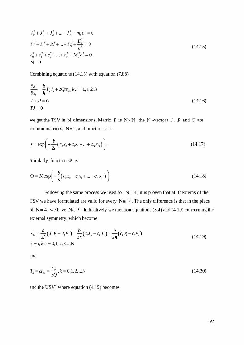
162

2 2 2 2 2 2

0 1 2 0

22 2 2 2 0

0 1 2 2

2 2 2 2 2 2

0 1 2 0

... 0

... 0

... 0

J J J J m c

EP P P P

c

c c c c M c

. (14.15)

Combining equations (14.15) with equation (7.88)

, , 0,1,2,3

0

ik i ki

k

J bP J zQ k i

x

J P C

TJ

(14.16)

we get the TSV in dimensions. Matrix T is , the -vectors J , P and C are

column matrices, 1 , and function z is

0 0 1 1exp ...2

bz c x c x c x

. (14.17)

Similarly, function is

0 0 1 1exp ...b

K c x c x c x

(14.18)

Following the same process we used for 4 , it is proven that all theorems of the

TSV we have formulated are valid for every . The only difference is that in the place

of 4 , we have . Indicatively we mention equations (3.4) and (4.10) concerning the

external symmetry, which become

2 2 2

, , 0,1,2,3,...

ki k i i k i k k i k i i k

b b bJ P J P c J c J c P c P

k i k i

(14.19)

and

, 0,1,2,...kkk kkT k

zQ

(14.20)

and the USVI where equation (4.19) becomes

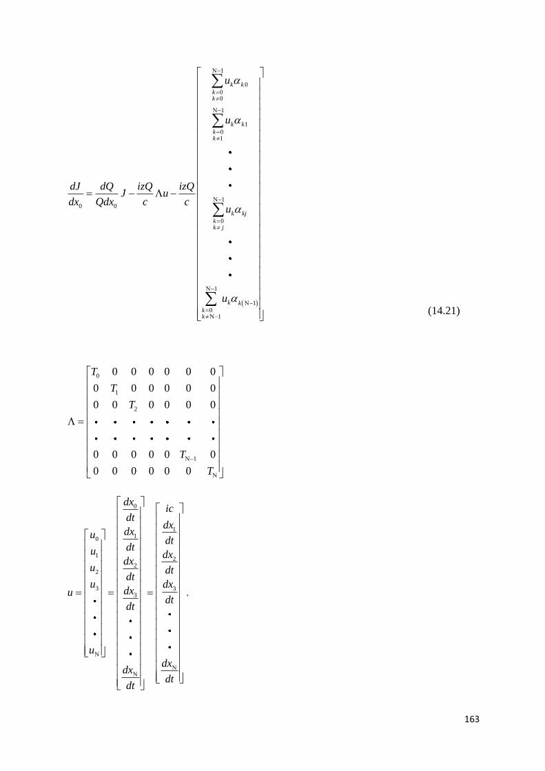
163

1

0

00

1

1

01

10 0

0

1

10

1

k k

kk

k k

kk

k kj

kk j

k kkk

u

u

dJ dQ izQ izQJ u

dx Qdx c cu

u

(14.21)

0

1

2

1

0 0 0 0 0 0

0 0 0 0 0 0

0 0 0 0 0 0

0 0 0 0 0 0

0 0 0 0 0 0

T

T

T

T

T

0

11

0

12

22

3 33

dxic

dtdx

dxudt

dtu dxdx

u dtdt

u dxdxu

dtdt

u

dxdx

dtdt

.

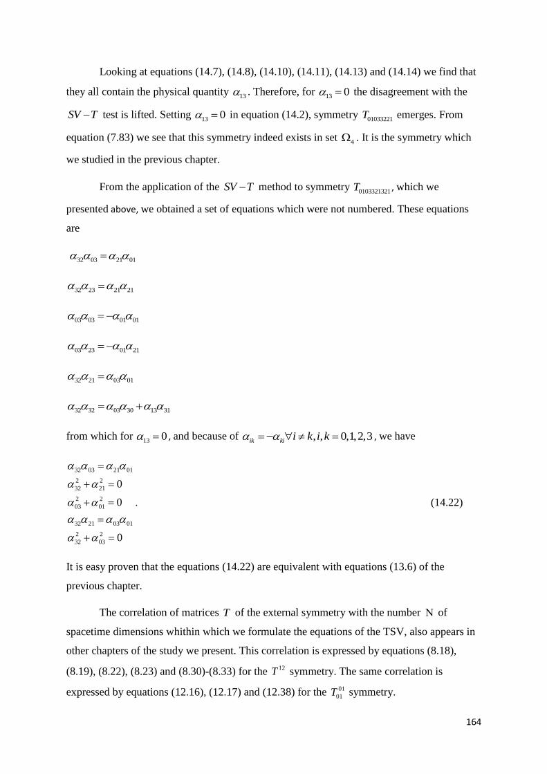
164

Looking at equations (14.7), (14.8), (14.10), (14.11), (14.13) and (14.14) we find that

they all contain the physical quantity 13 . Therefore, for

13 0 the disagreement with the

SV T test is lifted. Setting 13 0 in equation (14.2), symmetry

01033221T emerges. From

equation (7.83) we see that this symmetry indeed exists in set 4 . It is the symmetry which

we studied in the previous chapter.

From the application of the SV T method to symmetry 0103321321T , which we

presented above, we obtained a set of equations which were not numbered. These equations

are

32 03 21 01

32 23 21 21

03 03 01 01

03 23 01 21

32 21 03 01

32 32 03 30 13 31

from which for 13 0 , and because of , , 0,1,2,3ik ki i k i k , we have

32 03 21 01

2 2

32 21

2 2

03 01

32 21 03 01

2 2

32 03

0

0

0

. (14.22)

It is easy proven that the equations (14.22) are equivalent with equations (13.6) of the

previous chapter.

The correlation of matrices T of the external symmetry with the number of

spacetime dimensions whithin which we formulate the equations of the TSV, also appears in

other chapters of the study we present. This correlation is expressed by equations (8.18),

(8.19), (8.22), (8.23) and (8.30)-(8.33) for the 12T symmetry. The same correlation is

expressed by equations (12.16), (12.17) and (12.38) for the 01

01T symmetry.

165

The equations of the TSV apply when, in equation (14.15), at least one component of

the momentum J is non-zero. Therefore, the TSV is formulated for every . By

induction we can conclude that the equations of the TSV are also valid for .

15. THE SET 6

15.1. Introduction

In this chapter we determine the basic characteristics of the 010203321321T symmetry of

set 6 . It is the only symmetry in which all physical quantities , , , 0,1,2,3ki k i k i are

non-zero.

As is the case in the symmetries of set 4 , the rest masses

0m , 0

2

E

c and

0M vanish,

00 02

0E

m Mc

. The same is true for the four-vector j of the density of the conserved

quantities of the generalized particle, which is 0j . Additionally, the generalized particle is

always in the form of the generalized photon. On top of this, the 010203321321T symmetry has

two properties not shared by any other symmetry of the set 1 2 3 4 . The first is

that the vectors n and τ of equations (7.24), (7.23) are equal or opposite, τ n 0 . The

second property, which is a consequence of the first, is that the fundamental matrices M and

N are equal or opposite, M N .

In some of the equations we present, the symbol appears. In these equations, either

all of the ¨up¨ or all of the ¨down¨ signs apply. For τ n the up signs apply, while for

τ n the down.

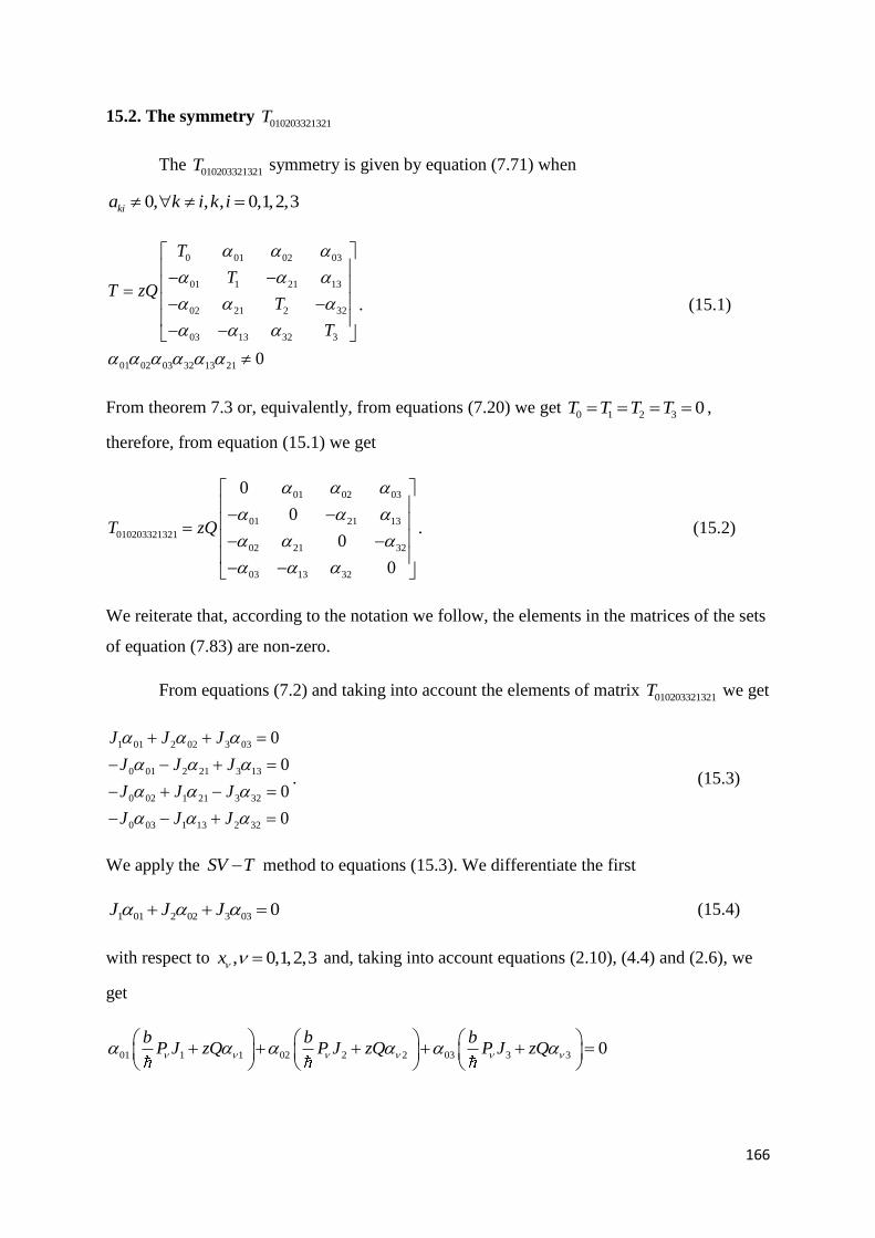
166

15.2. The symmetry 010203321321T

The 010203321321T symmetry is given by equation (7.71) when

0, , , 0,1,2,3kia k i k i

0 01 02 03

01 1 21 13

02 21 2 32

03 13 32 3

01 02 03 32 13 21 0

T

TT zQ

T

T

. (15.1)

From theorem 7.3 or, equivalently, from equations (7.20) we get 0 1 2 3 0T T T T ,


01 02 03

01 21 13

010203321321

02 21 32

03 13 32

0

0

0

0

T zQ

. (15.2)

We reiterate that, according to the notation we follow, the elements in the matrices of the sets

of equation (7.83) are non-zero.

From equations (7.2) and taking into account the elements of matrix 010203321321T we get

1 01 2 02 3 03

0 01 2 21 3 13

0 02 1 21 3 32

0 03 1 13 2 32

0

0

0

0

J J J

J J J

J J J

J J J

. (15.3)

We apply the SV T method to equations (15.3). We differentiate the first

1 01 2 02 3 03 0J J J (15.4)

with respect to , 0,1,2,3x and, taking into account equations (2.10), (4.4) and (2.6), we

get

01 1 1 02 2 2 03 3 3 0b b b

P J zQ P J zQ P J zQ

167

1 01 2 02 3 03 01 1 02 2 03 3 0b

P J J J zQ


01 1 02 2 03 3 0zQ

and because 0zQ we get

01 1 02 2 03 3 0 . (15.5)

Setting successively 0,1,2,3 into equation (15.5) we get:

For 0 ,

2 2 2

01 02 03 0a a a . (15.6)

For 1 ,

01 11 02 12 03 13

01 1 02 21 03 13

02 21 03 13

03 13 02 21

0

0

0 0

T

a a a a

a a a a

13 21

02 03

a a

a a . (15.7)

For 2 ,

01 21 02 22 03 23

01 21 02 2 03 32

01 21 03 32

01 21 03 32

0

0

0 0

a a a a a a

a a a T a a

32 21

01 03

. (15.8)

For 3 ,

168

01 31 02 32 03 33

01 13 02 32 03 3

01 13 02 32

01 13 02 32

02 32 01 13

0

0

0 0

0

T

32 13

01 02

. (15.9)

From equations (15.7), (15.8), (15.9) we get

32 13 21

01 02 03

. (15.10)


3 13 0 01 2 21J J J (15.11)

and differentiating with respect to , 0,1,2,3x and, taking into account equations (2.10)

and (4.4), we get

13 3 3 01 0 0 21 2 2

b b bP J zQ P J zQ P J zQ

3 13 13 3 0 01 2 21 01 0 21 2

b bP J zQ P J J zQ


13 3 01 0 21 2zQ zQ

and because 0zQ we get

13 3 01 0 21 2 . (15.12)


For 0 ,

169

13 03 01 00 21 02

13 03 01 0 21 02

13 03 21 02

13 03 21 02

0

T

13 21

02 03

a a

a a


For 1 ,

13 13 01 10 21 12

2 2 2

13 01 21

2 2 2

13 21 01

2 2 2

01 13 21 0 . (15.13)

For 2 ,

13 23 01 20 21 22

13 23 01 20 21 2

13 23 01 20

T

32 13 01 02 . (15.14)

For 3 ,

13 33 01 30 21 32

13 3 01 03 32 21

01 03 32 210

T

01 03 32 21 . (15.15)

From equations (15.6), (15.10), (15.13), (15.14) and (15.15) we get

32 13 21

01 02 03

2 2 2 2 2 2

01 02 03 32 13 21

1

0

. (15.16)

Similarly, the application of the SV T method to the third and fourth of equations (15.3),

always gives either one of the first or one of the second of the equations (15.16).

170

From equations (15.16) and (7.23), (7.24) we get

τ n 0

32 01

13 02

21 03

. (15.17)


01 02 03

01 03 02

010203321321

02 03 01

03 02 01

0

0

0

0

T zQ

. (15.18)

Equation (15.18) gives the two mathematical expressions of matrix 010203321321T .

From the second of equations (4.6) for , , 0,1,2 , 0,1,3 , 0,2,3 , 1,2,3i k we

get

0 12 2 01 1 20

0 13 3 01 1 30

0 23 3 02 2 30

1 23 3 12 2 31

0

0

0

0

J J J

J J J

J J J

J J J

0 21 2 01 1 02

0 13 3 01 1 03

0 32 3 02 2 03

1 32 3 21 2 13

0

0

0

0

J J J

J J J

J J J

J J J

. (15.19)

It is easy to prove that equations (15.19) and (15.3) are equivalent if we consider the first of

equations (15.16). Consequently, for the calculation of the momenta 0 1 2 3, , ,J J J J we have at

our disposal four independent equations.

Equations (15.19) constitute a 4 4 linear homogeneous system with the momenta

0 1 2 3, , ,J J J J as unknowns. The determinant, as well as all the 3 3 subdeterminants of the

system are equal to zero, while the 2 2 subdeterminants are non-zero. Consequently, there

are two independent variables in the sytem. If we consider as independent variables the

momenta 0 1,J J we get the solution

171

03 132 0 1

32 32

02 213 0 1

32 32

J J J

J J J

(15.20)

03 13

0 1

32 32

02 21

3232

1 0

0 1

J J J

. (15.21)


0 12 2 01 1 20

0 13 3 01 1 30

0 23 3 02 2 30

1 23 3 12 2 31

0

0

0

0

c c c

c c c

c c c

c c c

0 21 2 01 1 02

0 13 3 01 1 03

0 32 3 02 2 03

1 32 3 21 2 13

0

0

0

0

c c c

c c c

c c c

c c c

. (15.22)

Equations (15.22) constitute a 4 4 linear homogegeous system with the constants

0 1 2 3, , ,c c c c as unknowns. System (15.22) has the constants 0 1 2 3, , ,c c c c in place of the

momenta 0 1 2 3, , ,J J J J . Thus, it gives the solution corresponding to equation (15.19)

03 13

0 1

32 32

02 21

3232

1 0

0 1

C c c

(15.23)

where 0 1,c c , are independent parameters.

In the 010203321321T symmetry it is 0, , , 0,1,2,3kia k i k i , therefore, from

equations (3.4) and (4.4) we get

172

, , , 0,1,2,3k i i kc J c J k i k i . (15.24)

From relation (15.24) for , 0,1k i we get

0 1 1 0c J c J . (15.25)

From relation (15.25) emerges that the four-vectors J and C of equations (15.21) and

(15.23) cannot be parallel.

The four-vectors J and C have additional mathematical expressions other than

(15.21) and (15.23). These expressions emerge if we allow two other pairs of free parameters

in systems (15.19) and (15.22). All the mathematical expressions arising from the systems

(15.19) and (15.22) are equivalent to each other. The four-vector P is calculated from

equation (3.5)

P C J (15.26)

and equations (15.21) and (15.23).

From equation (2.7) and equation (15.21) we get

2 2

2 2 2 203 13 02 210 1 0 1 0 1 0

32 32 32 32

0J J J J J J m c

2 22 2 2 203 13 03 130 1 0 1 0 12 2 2

32 32 32

2 22 2 2 202 02 21210 1 0 1 02 2 2

32 32 32

2

20

J J J J J J

J J J J m c

and since, as follows from equation (15.16), is is 03 13 02 21 , we get

2 2 2 22 2 2 2 2 2 2 203 13 02 210 1 0 1 0 1 02 2 2 2

32 32 32 32

0J J J J J J m c

2 2 2 2 2 2 2 2 2 2

0 32 03 02 1 32 13 21 02

32

10J J m c

and since, as follows from equation (15.16), is is 32 01 , we get

2 2 2 2 2 2 2 2 2 2

0 01 03 02 1 32 13 21 02

32

10J J m c

173


2 2

00 0m c

0 0m . (15.27)

Similarly, from equations (3.6) and (15.23) we get

0 0M (15.28)

and from (2.8) and (15.26) we get

0 0E . (15.29)




In the preceding study we denoted J the four-vector J Q . Knowing four-vector

J Q we can calculate the four-vectors J and P from equations (7.86). The calculation of

the four-vectors J and P can also be made through equations (11.6), (11.7) and (11.16). We

note that in the 010203321321T symmetry, equation (11.18) applies, since it can be

0 1 0c c .


0 1 2 3 0T T T T , therefore, from equation (4.11)

we get 0 , and from equation (7.73) of theorem 7.5 we get

2bcj MC

. (15.30)

Taking into account equations (15.16) we get from equations (4.28) and (7.3) equation

N M (15.31)

for the fundamental matrices M and N in the 010203321321T symmetry. From equations (15.30)

and (15.31) we get

2bcj NC

and with the first of equations (7.4) we get

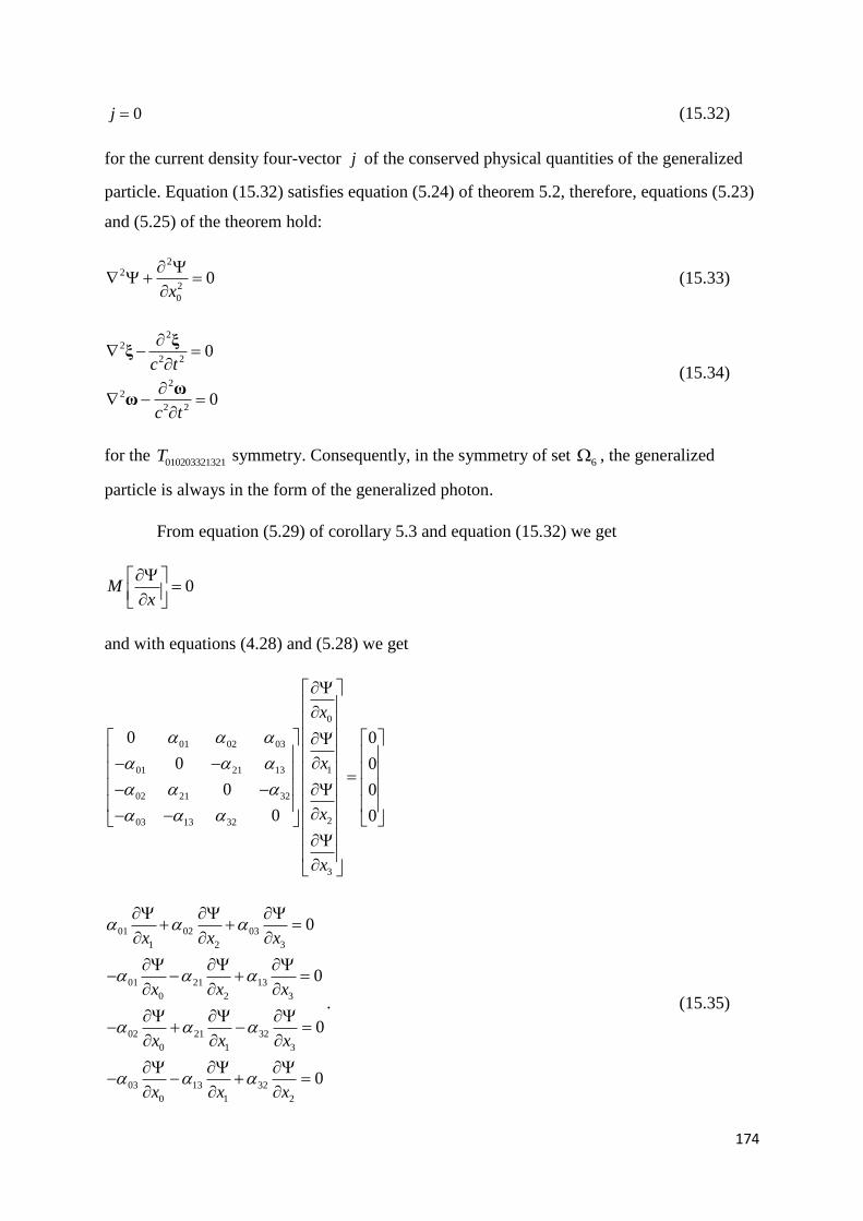
174

0j (15.32)

for the current density four-vector j of the conserved physical quantities of the generalized

particle. Equation (15.32) satisfies equation (5.24) of theorem 5.2, therefore, equations (5.23)

and (5.25) of the theorem hold:

22

2

0

0x

(15.33)

22

2 2

22

2 2

0

0

c t

c t

ξξ

ωω

(15.34)

for the 010203321321T symmetry. Consequently, in the symmetry of set

6 , the generalized

particle is always in the form of the generalized photon.

From equation (5.29) of corollary 5.3 and equation (15.32) we get

0Mx


0

01 02 03

101 21 13

02 21 32

203 13 32

3

0 0

0 0

0 0

0 0

x

x

x

x

01 02 03

1 2 3

01 21 13

0 2 3

02 21 32

0 1 3

03 13 32

0 1 2

0

0

0

0

x x x

x x x

x x x

x x x

. (15.35)

175

Equations (15.35) constitute a 4 4 linear homogeneous system with unknowns

, 0,1,2,3k

kx

. The determinant as well as all of the 3 3 subdeterminants of the system

are zero. The 2 2 subdeterminants of the system are non-zero. Therefore, there are two

independent variables in the system. If we set 0 1

,x x

as independent variables, we get the

solution

03 13

2 32 0 32 1

02 21

3 32 0 32 1

x x x

x x x


03 02

2 01 0 01 1

02 03

3 01 0 01 1

x x x

x x x

. (15.36)

Now the calculation of 0 1

,x x

is performed through equation (5.3)

0 0 0 0

0

1 1 1 1

1

b bJ P J c

x

b bJ P J c

x

(15.37)

where we necessarily introduce the degrees of freedom , of the TSV.

From equations (7.26), (7.27) and (15.17) we get

ic

i

c

ξ ω

ω ξ (15.38)

for the symetry 010203321321T . Field ω emerges from field ξ through rottation by angle

2

,

considering vectors ξ and ω on the complex plane. The sign of angle 2

is opposite from the

one in equation (15.17), according to the way in which we use the symbol.

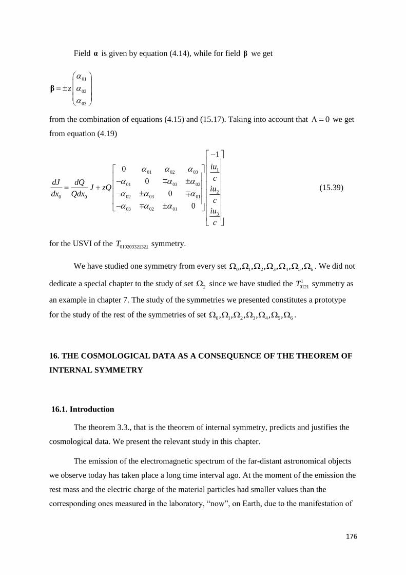
176

Field α is given by equation (4.14), while for field β we get

01

02

03

z

β

from the combination of equations (4.15) and (15.17). Taking into account that 0 we get

from equation (4.19)

101 02 03

01 03 02

202 03 010 0

03 02 013

1

0

0

0

0

iu

cdJ dQ

J zQ iudx Qdx

c

iu

c

(15.39)

for the USVI of the 010203321321T symmetry.

We have studied one symmetry from every set 0 1 2 3 4 5 6, , , , , , . We did not

dedicate a special chapter to the study of set 2 since we have studied the 1

0121T symmetry as

an example in chapter 7. The study of the symmetries we presented constitutes a prototype

for the study of the rest of the symmetries of set 0 1 2 3 4 5 6, , , , , , .

16. THE COSMOLOGICAL DATA AS A CONSEQUENCE OF THE THEOREM OF

INTERNAL SYMMETRY

16.1. Introduction

The theorem 3.3., that is the theorem of internal symmetry, predicts and justifies the

cosmological data. We present the relevant study in this chapter.

The emission of the electromagnetic spectrum of the far-distant astronomical objects

we observe today has taken place a long time interval ago. At the moment of the emission the

rest mass and the electric charge of the material particles had smaller values than the

corresponding ones measured in the laboratory, “now”, on Earth, due to the manifestation of

177

the Selfvariations. The consequences resulting from this difference are recorded in the

cosmological data. The cosmological data have a microscopic and not a macroscopic cause.

Due to the Selfvariations of the rest masses of the material particles the gravitational

interaction cannot play the role attributed to it by the Standard Cosmological Model (SCM).

The gravitational interaction cannot cause neither the collapse, nor the expansion of the

universe, since it decreases on a cosmological scale according to the factor 1

1 z. The

gravitational interaction exercised on our galaxy by a far-distant astronomical object with

redshift 9z is only the 1

10 of the expected one. The universe is static and flat, according

to the law of Selfvariations.

16.2. The Cosmological Data as a Consequence of the Theorem of Internal Symmetry

For a non- moving particle, that is for 1 2 3 0J J J , from equation (3.12) we get

that 1 2 3 0c c c and from equation (3.9) we obtain

0 0expb

K c x

and since 0x ict , we have

0expicc

K t

and from equation (3.10) we obtain

00 0

01 exp

Mm m t

iccK t

. (16.1)

The rest mass 0m of the material particle is a function of time t .

We now denote by k the constant

0icck

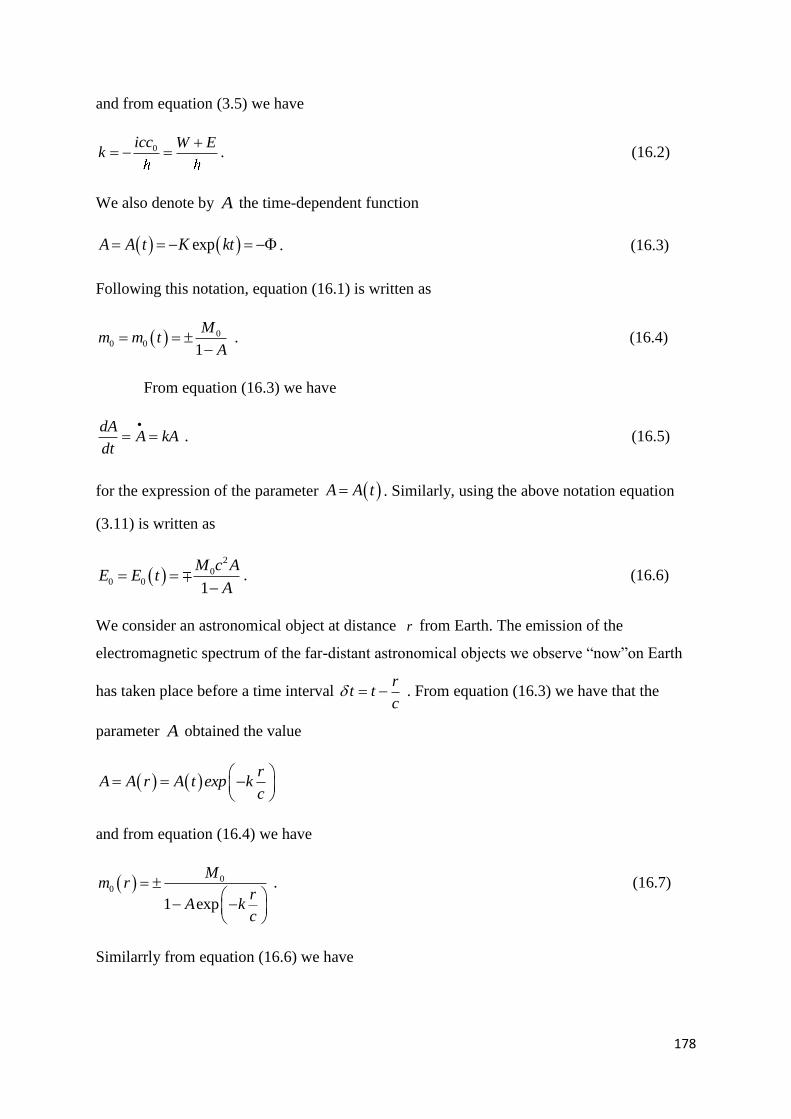
178


0icc W Ek

. (16.2)

We also denote by A the time-dependent function

expA A t K kt . (16.3)

Following this notation, equation (16.1) is written as

00 0

1

Mm m t

A

. (16.4)


dAA kA

dt

. (16.5)

for the expression of the parameter A A t . Similarly, using the above notation equation

(3.11) is written as

2

00 0

1

M c AE E t

A

. (16.6)

We consider an astronomical object at distance r from Earth. The emission of the

electromagnetic spectrum of the far-distant astronomical objects we observe “now”on Earth

has taken place before a time interval r

t tc

. From equation (16.3) we have that the

parameter A obtained the value

r

A A r A t exp kc


00

1 exp

Mm r

rA k

c

. (16.7)

Similarrly from equation (16.6) we have

179

2

0

0

exp

1 exp

rM c A k

cE r

rA k

c

. (16.8)


0 0

1

1 exp

Am r m

rA k

c

. (16.9)

We can prove that for the electric charge q of the material particles an equation

analogous to equation (16.7) is valid. From equation (4.2) we derive an equation

corresponding to equation (16.9), which is the following equation

1

1

1 exp

Bq r q

rB k

c

. (16.10)

The fine structure constant is defined as

2

04

q

c

(16.11)

and using equation (16.10) we obtain

2

1

1

1 exp

Br

rB k

c

. (16.12)

The wave length of the linear spectrum is inversely proportional to the factor 4

0m q ,

where 0m is the rest mass and q is the electric charge of the electron. If we denote by 0 the

wavelength of a photon emitted by an atom “now”on Earth, and by the same wavelength of

the same atom received “now” on Earth from the far-distant astronomical object, the

following relation holds:

4

0

4

0 0

m q

m r q r

and from equations (16.9) and (16.10) we obtain

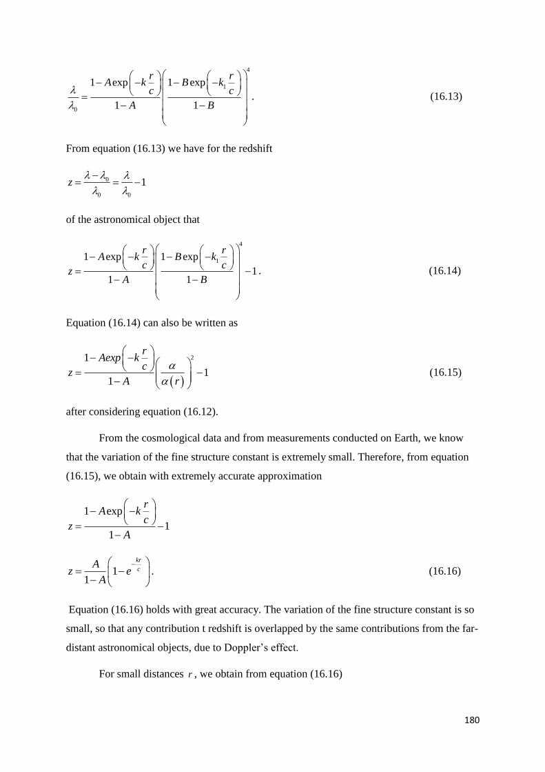
180

4

1

0

1 exp 1 exp

1 1

r rA k B k

c c

A B

. (16.13)

From equation (16.13) we have for the redshift

0

0 0

1z

of the astronomical object that

4

11 exp 1 exp

11 1

r rA k B k

c cz

A B

. (16.14)

Equation (16.14) can also be written as

21

11

rAexp k

cz

A r

(16.15)

after considering equation (16.12).

From the cosmological data and from measurements conducted on Earth, we know

that the variation of the fine structure constant is extremely small. Therefore, from equation

(16.15), we obtain with extremely accurate approximation

1 exp

11

rA k

cz

A

11

kr

cA

z eA

. (16.16)

Equation (16.16) holds with great accuracy. The variation of the fine structure constant is so

small, so that any contribution t redshift is overlapped by the same contributions from the far-

distant astronomical objects, due to Doppler’s effect.

For small distances r , we obtain from equation (16.16)

181

1 11

1

A krz

A c

kAz r

c A

and comparing this with Hubble’s law

cz Hr

we get

1

kAH

A

(16.17)

where H is Hubble’s parameter.


2

1

1

k A A kA AdHH

dt A

2

1

k AH

A


2

21

k AH

A


HH

A

. (16.18)

For 2

0 0

2 2

0 0

0 0m c E

M c M c or

2

0 0

2 2

0 0

0 0m c E

M c M c we have

2

0 0

2 2

0 0

0m c E

M c M c


182

2

01

0

and with equation (16.3) we finally get

0

0A

. (16.19)


01

kA

A

and considering relation (16.19) we get two combinations for the constant k and the

parameter A :

0 1 0 0 1 1 0

1 0 1 0 0

A k k

A k k

. (16.20)

From equations (16.7) and (16.8) it follows that the sign change of the constant k is

equivalent with the interchange of the roles of the rest masses 0m and 0

2

E

c . Hence it suffices

to present the conclusions resulting from the first case of (16.20).

For 0k for equation (16.16) we have

lim1r

Az

A

. (16.21)

The redshift has an upper limit which depends on the value of the parameter A , even in the

case that the universe extends to infinity. In the case the universe has finite extension, let

maxr R and from equation (16.16) we have

max 11

kR

cA

z eA

. (16.22)

Thus redshift has a maximum value. The upper redshift limit of equation (16.21) and maxz of

equation (16.22) are almost equal. Hence in the following we will use equation (16.21).

From equations (16.16) and (16.5) we get after the calculations

183

2

11

kr

cdz kA

z edt A


1 01

kr

cH H

z e zA A

. (16.23)

Thus the redshift of far distant astronomical objects increases slightly with the passage of

time.

According to equation (16.21) it is

1

Az

A

and because of 1 0A we have

1

zA

z

and because of 1A we have

11

zA

z

. (16.24)

From the inequality (16.24) it follows that

1A . (16.25)

We prove now that as 1A the equation (16.16) tends to Hubble’s law cz Hr . Let

1 Ax

A

then 0x for 1A , while from equation (16.17) we get k xH and

equation (16.16) may be written as

11 exp

Hrz

x c

.

Hence we get

1 0

1lim lim 1 expA x

Hr Hrz x

x c c

.

184

From relation (16.5) follows the conclusion that

0dA

kAdt

. (16.26)

Thus the parameter A increases with the passage of time. Hence according to the

forementioned proof, the equation (16.16) tends to the Hubble law with the passage of time.

Combining equations (16.9) and (16.16) we have

00

1

mm z

z

. (16.27)

The equation (16.27) has multiple consequences on cosmological scale.

According to equation (16.27) the gravitational interaction between two astronomical

objects is smaller than expected by the factor 1

1 z. The redshift z depends on their distance

r as given in equation (16.16). This is the redshift that an observer on one object would

measure by observing the other object.

For the solar system or for the structure of a galaxy or a galaxy cluster, equation

(16.27) has no consequences. On this distance scale we practically have 0z . However we

can seek consequences on this scale from another equation. From equation (16.4) we have

0

0 21

odm M Am

dt A


0 01

Am m

A


0

0 1

m kA

m A


185

0

0

mH

m

(16.28)

for the rest mass of the electron.

Equation (16.28) concerns the mass 0 0m m t . Therefore its consequences can be

found in our galaxy or even in the solar system. We notice that the value of the Hubble

parameter H is probably smaller than the one accepted today, but we will not continue the

analysis to this matter in this publication. In any case the experimental verification of

equation (16.28) requires measurements with sensitive instruments of observation. For the

conduct of these measurements equation (4.19) of the USVI must also be taken into account.

Equation (16.27) has important consequences on cosmological scale distances. For

such distances the gravitational interaction diminishes quickly and beyond some distance it

practically vanishes. It has however played an important role for the creation of all large

structures in the universe.

As we will see further down, the very early universe differed only slightly from

vacuum. The gravitational interaction strengthens with the passage of time, as the rest masses

of material particles increase. Moreover, its strength depends on distance as predicted by the

law of universal gravitation, but also for cosmological distances, as predicted by equation

(16.27). Both these factors played an important role for the creation of all large structures in

the universe and have not been both accounted for in the interpretation of the cosmological

data via the SCM.

From equations 2E mc and (16.27) we have

1

EE z

z

. (16.29)

In every case of transformation of mass to energy. The production of energy in the universe is

mainly achieved via hydrogen fusion and nuclear reactions. Therefore the energy produced in

the past in the far distant astronomical objects was smaller than the corresponding energy

produced today in our galaxy through the same mechanism. This fact has two immediate

consequences.

The first is that equation (16.16) is valid for the redshift az of the radiation which

stems from accelerated / decelerated electrons

186

11

kr

ca

Az e

A

. (16.30)

And hence for the continuous spectrum. Similar mechanisms which accelerate electrons in

our galaxy and in far distant astronomical objects do not give the same amount of energy to

the electrons. According to equation (16.29) the energy which is supplied to the electrons in

far distant astronomical objects is less than the corresponding energy in our galaxy.

The second consequence concers the luminosity distance D of far distant astronomical

objects. The overall decrease of the energy produced in the past, due to equation (16.29) has

as consequence the overall decrease of luminositites of distant astronomical objects. From the

definition of the luminosity distance D it follows easy that

1D r z . (16.31)

Between the distance r of the astronomical object and the distance D measured from its

luminosity. The luminosity distance D is measured always larger than the real distance of the

astronomical object. The real distance r of the distant astronomical object is given by eq.

ln

1 1

c Ar

k z A

(16.32)

which follows from equation (16.16). The distance measurement from equation (16.32) can

be made if we know the constant k and the parameter A . Generally, due to equation (16.17)

it suffices to know two of the parameters , ,k A H .

The ionization energy as well as the excitation energynX of atoms is proportional to

the factor 4

0m q , where 0m is the rest mass and q the electric charge of the electron. Hence we

get

4

0

0

n

n

X r m r q r

X m q

2

0

0

n

n

X r m r r

X m

and because of

187

1r

we have

0

0

n

n

X r m r

X m


1

1

n n

n n

X r X z

X X z

1

nn n

XX r X z

z

. (16.33)

From equation (16.33) we conclude tha the ionization and excitation energies of atoms

decrease with inceasing redshift. This fact has consequences on the degree of ionization of

atoms in the distant astronomical objects

The number of excited atoms in a gas in a state of thermodynamic equilibrium is

given by Boltzmann’s eq.

1 1

expn n nN g X

N g KT

(16.34)

where nN is the number of atoms at energy level n ,

nX the excitation energy from the the

1st to the nth energy level, 23 11.38 10K JK Boltzmann’s constant, T the temperature in

degrees Kelvin, and ng the multiplicity of level n , i.e. the number of levels into which level

n is split apart inside a magnetic field.

Combining equations (16.33) and (16.34) we get

1 1

exp1

n n nN g X

N g KT z

. (16.35)

For the hydrogen atom for 19

2 1 22, 10.5 16.4 10 , 2, 8n X eV J g g and at the surface

of the Sun where 6000T K equation (16.34) implies that just one in 810 atoms is at state

188

2n . Correspondingly from equation (16.35) and for 1z we have 42

1

2.2 10N

N

, for

2z we have 32

1

5.8 10N

N

, and for 5z we have 2

1

0.15N

N .

Considering eq. (16.21) we get from equation (16.33)

1n nX r X A . (16.36)

Considering relations (16.24) and (16.25) we conclude that the ionization and excitation

energies of atoms tend to zero in the very early universe. The universe went through an

ionization phase in its initial phase of evolution.

The laboratory value of the Thomson scattering coefficient is given by equation

4

2 4

0

8

3

q

m c

(16.37)

where 0m the rest mass and q the electric charge of the electron. Thus we have

2

0

0

T

T

z m

m z z

and because of z we get

2

0

0

T

T

z m

m z


21

T

T

zz

. (16.38)

The Thomson coefficient concerns the scattering of photons with low energy E . For

photons with high energy E the photon scattering is determined from the Klein-Nishina

coefficient :

0

2

0

3 2 1ln

8 2T

m E

E m c

(16.39)

189

in the laboratory and

2

0

2

0

23 1ln

8 2T

m z c E zz z

E z m z c

(16.40)

in astronomical objects with redshift z . From equations (16.27) and (16.29) we have

0 0

m z m

E z E

hence from equation (16.40) we get

2

0

2

0

3 2 1ln

8 2T

m c Ez z

E m c


21

T

T

z zz

. (16.41)

From equation (16.41) we conclude that the Thomson and Klein-Nishina scattering

coefficients increase with redshift and indeed in the same manner. Considering equation

(16.21) we have

2

1

1

T

T

r r

A

. (16.42)

Considering equations (16.24) and (16.25) we conclude that the Thomson and Klein-Nishina

scattering coefficients had enormous values in the vary early universe. In its initial phase the

universe was totally opaque. From this initial phase stems the cosmic microwave background

radiation (CMBR) we observe today.

The internal symmetry theorem (3.3) predicts that the initial universe was at a

‘vacuum state’ with temperature 0T K . Due to the Selfvariations the universe evolved to

the state we observe today. This evolution agrees with the fact that the CMRB corresponds to

a black body radiation with temperature 2.73T K .

Combining equations (3.11) and (16.3) we have in the laboratory

190

, 0,1,2,3

1

ii

cJ i

A t

and

, 0,1,2,3

1 1 exp

i ii

c cJ r i

r krA t A

c c

for an astronomical object at distance r , and combining these two equations with equation

(16.9) we get

0

0

i

i

J r m r

J m


1

1

i

i

J z

J z

, 0,1,2,31

ii

JJ z i

z

. (16.43)

From the Heisenberg uncertainty principle for the axis 1x x we have

1J x

in the lab, and

1J z x z

for the astronomical object, and combining these two relations we get

1 1J z x z J x


1x z z x . (16.44)

From equation (16.44) we conclude that the uncertainty x z of position of a

material particle increases with redshift. Moreover as the universe evolved towards the state

we observe today, the uncertainty of position of material particles was decreasing.

191


1

xx r

A

. (16.45)

Considering relations (16.24) and (16.25) we conclude that in the very early universe there

existed great uncertainty of position of material particles. The same conclusions arise for the

Bohr radius. The TSV is agrees with the uncertainty principle. In the next chapter we will see

that the uncertainty of position of a material particle is one more consequence of theorem 3.3.

From equation (16.33) it follows that as the universe evolved to the state we observe

today the ionization energy increased. This prediction is generally valid for any kind of

negative dynamical energies which bind together material particles to produce more complex

particles. From equation (16.27) we have

2

2 00

1

m cm z c

z

(16.46)

for the energy 2

0m c , the mass deficiency, which ties together the particles which constitute

the nuclei of the elements. According to equation (16.46) the energy 2

0m c , like the

ionization energies, increased as the universe evolved towards its present state.

Particle like the electron, which today are considered fundamental may in fact be

composed of other particles. Our inability to break them apart could be due to the

strengthening of the binding energies of the constituent particles. The mass0M in equation

(3.10) has many chances to the only realy fundamental rest mass, from which the masses of

all other particles are composed.


0 0 1 0m r m A . (16.47)

Considering the relations (16.24) and (16.25) we conclude that, towards the initial state of

the universe, the rest masses of material particles tend to zero:

0 0 1 0m r m A . (16.48)


0 0E r . (16.49)

192

According to the relations (16.48) and (16.49) the initial state of the universe slightly differed

from vacuum. The same conclusion arises in the case the universe is finite, taking

maxr R instead of the condition r we have used.

We have studied the case of 1 2 3 0J J J in equation (3.12) in order to bypass the

consequences on the redshift produced by the proper motion of the electron. Thus, from


00

icM

c .

From equation (16.2) we also have

0 2

kM

c . (16.50)

From equation (16.17) we obtain that the constant k obtains an extremely small value.

Therefore, the same holds and for the rest mass 0M , as a result of equation (16.50).

From equation (16.5) we conclude that the parameter Avaries only very slightly with the

passage of time. The age of the Universe is correlated at a greater degree with the value of the

parameter A we measure today, and less with Hubble’s parameter H . In any case the two

parameters Aand H are correlated via equation (16.17).

With the exception of equations (16.16) and (16.32), the TSV equations for

cosmology do not depend on the values of the parameters k , A and H . They solely depend

on z , which is accurately measured. Equation (16.27) allows us to express all the

fundamental astrophysical equations as a function of z . For measurements with higher

accuracy, and whenever allowed by the observation instruments, we have to consider

equations (16.10) and (16.12).

The redshift in equation (16.14) comes from the selfvariations of the rest mass and the

electric charge of the electron. The redshift in the main volume of the linear spectrum we

observe from distant astronomical objects, is actually caused by this effect. Today, however,

we have the capability [16] to perform high sensitivity measurements of the effects of the

Selfvariations. The structure of matter predicted by TSV must be taken into account in these

measurements. The fundamental rest mass 0M of equation (16.50) is by far smaller than the

neutrino mass. Neutrinos, not to speak of other particles, have internal structure. This

193

structure could influence the sum W E in the right part of equation (16.2). In such a case,

we will obtain a different value for the constants k and 0c for different material particles.

Writing equation (16.2) in the form

0, p p p

p

ic W Ek

(16.51)

we can introduce an index “ p ” in the equations of this chapter. Every index “ p ”

corresponds to a specific particle when the right part of equation (16.2) is not constant.

The measurements we perform on a cosmological scale depend on the physical

quantity

1

p p

p

p

k AH

A

. (16.52)

The main volume of the linear spectrum we get from distant cosmological objects comes

from the process of atomic excitation/relaxation, thus the Hubble parameter H as given by

equation (16.17)

1

kAH

A

expresses the consequences of the selfvariation of the electron rest mass. In equations

(16.14), (16.16), (16.22), (16.32), (16.33), (16.35), (16.41) and (16.42) the rest mass of the

electron comes into play. Therefore, these equations are unaffected by equation (16.51).

The energy of the radiation that comes from nuclear reactions, and not from

accelerated/decelerated electrons, depends on the particles that take part in the reaction.

Consequently, their energy depends on equation (16.51). In this case equation (16.9) takes the

form

0 0

1

1 exp

p

p p

Am r m

rA k

c

(16.53)

and considering that

2

0

2

0

r m c

m r c

194

we get

1 exp

1

p p

p

rA k

r c

A

and we finally get

1 exp1

p

p

p

A rz k

A c

. (16.54)

For relatively small distances, from equation (16.54) we get

1

p p

p

p

k A r rz H

A c c

. (16.55)

Correlating a source of radiation from nuclear reactions with a galaxy, we can compare the

z and z redshifts. From this comparison we can draw important conclusions about equation

(16.51) as well as about the predictions of the TSV. We note that the SCM, in explaining the

redshift through the hypothesis of universal expansion, does not predict any difference

between the z and z redshifts.

Equation (16.28)

0

0

mH

m

holds for the rest mass of the electron. For other particles it is written in the form

0

0 1

p p

p

p

k AmH

m A

. (16.56)

The mass of the electron represents a small part of the mass of the atom. Therefore, in

measurements based on the gravitational interaction, the consequences of the mass

selfvariation are governed by equation (16.56).

The rest mass 0,Hm of the hydrogen atom is

0, 0, 0,H p em m m (16.57)

195

where 0, pm and

0,em the rest mass of the proton and the electron respectively. From equation

(16.57) we have

0, 0, 0,H p em m m

and with equations (16.56) for the proton and (16.28) for the electron we have

0, 0, 0,H p p em H m Hm

. (16.58)


0, 0, 0,

0, 0, 0,

H p p e

H p e

H m Hmm

m m m

and considering that today it is

4

0, 0,5.4 10e pm m

we have

4

0, 0,0,

4

0, 0, 0,

4

0,0,

40, 0,

5.4 10

5.4 10

5.4 10

1 5.4 10

p p pH

H p p

p pH

H p

H m H mm

m m m

m H Hm

m m

40, 4

4

0,

5.4 105.4 10

1 5.4 10

H p

p

H

H HmH H

m

. (16.59)

From equation (16.59) we conclude that the ratio

0,

0,

H

H

m

m

of the hydrogen atom depends on the relation of the parameter pH for the proton with the

Hubble parameter H . Similarly we obtain

0, 4

0,

1 5.4 10a

p n

a

mH H H

m

(16.60)

196

for any atom, where is the atomic number and is the nucleon number of the atom.

Equations (16.59) and (16.60) is valid for relatively small distances, up to a few hundred kpc

. For larger distances we have to repeat the procedure of the proof using equations (16.9) and

(16.53) instead of (16.28) and (16.56).

Equation (16.51) affects equations (16.27) and (16.29), which are written in the form

00

1

mm z

z

(16.61)

1

EE z

z

. (16.62)

The energy produced in the past at distant astronomical objects was smaller than the

corresponding energy produced today in our galaxy. The production of energy in the universe

is mainly through hydrogen fusion and nuclear reactions. Therefore, equation (16.62) is of

greater accuracy than equation (16.29). Nevertheless, the selfvariation of the electron’s rest

mass played a defining role in the energy produced in the past at distant cosmological objects.

This is due to the fact that the fundamental astrophysical parameters depend on the rest mass

of the electron. These parameters, therefore, depend on the redshift z , and not on the z ,

according to equations (16.33), (16.35), (16.36), (16.41) and (16.42). The most characteristic

example concerns type a supernovae. The value of the rest mass of the electron, given as a

function of the redshift z from equation (16.27), plays a defining role at all phases of

evolution of a star undergoing type a supernovae. In any case it is obvious which of the

performed measurements are affected by redshift z and which by z .

It is very likely that there exists a small set of elementary particles with rest masses

0 2

pkM

c

and not just one elementary particle of rest mass

0 2

kM

c .

It seems improbable that the sum W E on the right side of equation (16.2) is not affected

by the internal structure of the generalized particles.

197

All of the presented consequences of theorem 3.3 are recorded within the

cosmological data [17-27]. For the confirmation of the predictions of the theorem for the

initial state of the Universe the improvement of our observational instruments is demanded.

We also recommend evaluating the data recorded in CMRB, based on the equations of the

TSV.

In the observations conducted for distances of cosmological scales, we observe the

Universe as it was in the past. That is, we observe directly the consequences of the

Selfvariations. We do not possess this possibility for the distances of smaller scales. The

cosmological data are the result of the immediate observation of the Selfvariations and their

consequences.

17. OTHER CONSEQUENCES OF THE THEOREM OF THE INTERNAL

SYMMETRY. THE SET

17.1. Introduction

The consequences of the theorem of the internal symmetry cover a wider spectrum,

than the one already stated for the cosmological data. In these, the consequences of the

dependence of the function on time 0x ict are recorded. The function , according to

equation (3.9), is a function of the set of the coordinates 0 1 2 3, , ,x x x x and also of the constants

0 1 2 3, , ,c c c c . Therefore function may change as a consequence of the change of the

constants 0 1 2 3, , ,c c c c . In this chapter we study the conditions under which such a change can

be. We come to the conclusion that the alteration of the constants 0 1 2 3, , ,c c c c implies an

uncertainty of position of the material particle.

The uncertainty of the material particle is predicted from the eqs. of the TSV for other

reasons as well. When the constant b of the law of Selfvariations is not a real number, when

b , the eqs. of the TSV do not determine the position of the material particle in

spacetime.

198

17.2. Other Consequences of the Theorem of the Internal Symmetry . The set

The function , according to equation (3.9), is a function of the set of the

coordinates and also of the constants 0 1 2 3 0 1 2 3, , , , , , ,x x x x c c c c and given as

0 1 2 3 0 1 2 3 0 0 1 1 2 2 3 3, , , , , , , expb

x x x x c c c c K c x c x c x c x

. (17.1)

As in the previous chapter, we refrain our study in the case of 1 0 , as included in

theorem 3.3. This case is equivalent with the relations 0C and 0P respectively.

Equations (3.10) and (3.11) express the rest mass 0m of the material particle and the

rest energy 0E as a function of

00

1

Mm

(17.2)

2

00

1

M cE

(17.3)

2 2

0 0 0E m c M c . (17.4)

In these equations the only constant is the rest mass 0M of the generalized particle.

Additionally the rest masses 0m and

0E depend on the constants 0 1 2 3, , ,c c c c , according to

equations (17.2), (17.3) and (3.9), in the following sense: For a constant rest mass 0M of a

generalized particle there are infinite values of the constants 0 1 2 3, , ,c c c c , i.e. infinite states of

the 4-vectorC , for which equation (3.6) is valid:

2 2 2 2 2 2

0 1 2 3 0c c c c M c . (17.5)

According to equation (3.12) the different states of the 4-vector C are equivalent with the

ability of the material particle to have different momentums at the same point 0 1 2 3, , ,A x x x x .

Therefore the evolution of the generalized particle depends on all physical quantities

0 1 2 3 0 1 2 3, , , , , , ,x x x x c c c c . We now deduce corollary 17.1 of theorem 3.3.

Corollary 17.1. ΄΄ The only constant physical quantity for a material particle is its total rest

mass 0M . The evolution of the Universe, or of a system of particles, or of one particle, does

199

not depend only on time. Its evolution is determined by the Selfvariations, as this

manifestation is expressed through the function .΄΄

Proof. Corollary 17.1 is an immediate consequence of theorem 3.3.

According to corollary 17.1, each material particle is uniquely defined from the rest mass 0M

of equations (17.2) and (17.3).

From equations (2.4), (2.5) and (3.5) , and since it holds that 0x ict , we can write

the function in the form

1 2 3 1 1 2 2 3 3, , , expb

t x x x K W E t c x c x c x

(17.6)

with the sum 0W E icc being constant. This equation gives as a function of time t ,

instead of the variable 0x ict .

In the afterword we present the reasons, according to which the TSV strenghtens at an

important degree the Theory of Special Relativity [28-29]. In contrast, the theorem of internal

symmerty highlights a fundamental difference between the TSV and the Theory of General

Relativity. According to equations (17.1) and (17.2), the physical quantity, which is being

introduced into the equations of the TSV and remains invariant with repsect to all systems of

reference, is the quantity given by

0 0 1 1 2 2 3 3

bc x c x c x c x . (17.7)

Therefore, the TSV studies the physical quantity , and not, the also invariant with respect

to all systems of reference, physical quantity of the four-dimensional arc length

2 2 2 22

0 1 2 3dS dx dx dx dx . (17.8)

This arc length is studied by the Theory of General Relativity. The study of 2dS can be

interpreted in the manner that the Theory of General Relativity is a macroscopic theory. On

the contrary, in the TSV a differentiation between the levels of the macrocosm and the

microcosm does not exist. In equations (3.12), and for the energy and the momentum of the

material particle,

200

, 0,1,2,31

ii

cJ i

the concept of velocity does not exist. With the exception of equations (4.19) and (4.20),

within the totality of the equations of the TSV we already presented, the concept of velocity

does not enter. As we will see in the following, theorem 3.3 which justifies the cosmological

data, predicts the uncertainty of the postion-momentum of the material particles. The

difference among these two theories is highlighted in a concrete manner by the comparison of

equations (17.7) and (17.8). In the first, spacetime appers together with the four-vector C .

The second equation refers only to spacetime.

We present an example which highlights the diffrences among these two theories. It is

the famous Twin Paradox. We consider that the reader is familiar with this thought

experiment, as well as the result of the Theory of General Relativity [30]. The Theory of

General Relativity predicts correctly the time difference in the time duration counted by the

two twins. On the other hand, according to corollary 17.1, this time difference does not

suffice for providing a difference in the evolution of the twins. The twins have the same

generalized particles, which acquire the same rest masses 0M , at the time they meet together.

At the beginning and at the end of the travel the two twins are identical. Einstein drives the

wrong conclusion, not because the Theory of General Relativity is wrong, but because he

regards that this time difference implies a different evolution of the twins. But, this is not a

characteristic of the Theory of General Relativity. This is a common characteristic of all the

physical theories preceding the TSV.

At this point let me commentate. Einstein refers to this thought experiment as the

“Twin Paradox”, and not as a consequence of the Theory of General Relativity. According to

my opinion, Einstein understood that something was missing from the Theory of General

Relativity. To this point advocates also his peristance for determining the cause of the

quantum phenomena.

General relativity has been experimentaly verified from a large number of

experiments. Moreover on a distance scale of a few hundred kpc its predictions are not

affected by equation (16.27). We expect that the combination of the two theories on this

distance scale will give important results for the physical reality.

201

We consider a generalized particle with rest mass 0M . The material particle of the

generalized particle (together with STEM) can be at the spacetime point 0 1 2 3, , ,A x x x x with

its energy-momentum having any value. According to equations (3.9) and (3.12) this can

happen only with the variation of the 4-vector C . For a generalized particle the rest mass0M

is constant, which means that through the variation of the 4-vector C , equation (17.5)

remains valid.


, , 0,1,2,3i i i

k k k

J P ck i

c c c

(17.9)


3

0

, 0,1, 2,3j

k j

jk kj k

cbx x k

c c

. (17.10)

Equations (17.9) and (17.10) remain valid for any variation of the 4-vectorC . We will know

prove the following corollary of theorem 3.3:

Corollary 17.2 ΄΄The variation of the 4-vectorC of a generalized particle with rest mass0M ,

2 2 2 2 2 2

0 1 2 3 0c c c c M c (17.11)

implies the variation of the 4-vectors J and P according to equations

3

0

1, , 0,1,2,3

1 1

ji i ik j

jk k kj k

cJ c cbx x k i

c c c

(17.12)

3

0

, , 0,1,2,31 1

ji i ik j

jk k kj k

cP c cbx x k i

c c c

.΄΄ (17.13)

Proof: From equation (17.11) it follows that any change of one of the constants

, 0,1,2,3kc k , induces a change to the others. Taking the derivatives with respect to

0, 0,1,2,3kc k we have

202

3

0

, 0, 0,1,2,3j

k j k

j kj k

cc c c k

c

. (17.14)

The corollary is then implied from the combination of the equations (3.12), (17.10) and

(17.9).

According to the relation (16.19) we have 0 , while according to the relations

(16.20) the physical quantity 1 can be a positive or negative number. Hence from

equations (17.12) and (17.13) we may determine the consequences for the material particle

depending on whether the rates of change of

, , , 0,1,2,3i i

k k

J Pk i

c c

are negative, positive or zero.

As the 4-vector C variates there arises an uncertainty for the position of the material

particle. Corollary 17.2 predicts many cases for this uncertainty. We will restrict ourselves to

one of them. For 0i

k

J

c

and 1 0 from equation (17.12) we have

3

0

0, , 0,1,2,31

ji ik j

jk kj k

cc cbx x k i

c c


3

0

0, , 0,1,2,3ji

i k j

jk kj k

cc bJ x x k i

c c

. (17.15)

From inequality (17.15) for , , 0,1,2,3i k k i we have

3

0

1 0, 0,1,2,3j

k k j

j kj k

cbJ x x k

c

and because 0 we have

203

3

0

, 0,1,2,3j

k j

j kj k

cJ x x k

c b

. (17.16)

In the case where

3

0

0j

j

j kj k

cx

c

(17.17)

from inequality (17.16) we have

, 0,1, 2,3

0

k kJ x kb

. (17.18)

From equations (3.12) and (3.13) it follows that , 0,1,2,3k kP J k , and considering that

0 we get from inequality (17.18) that

, 0,1,2,3k k

bP x k . (17.19)

The inequalities (17.16), (17.17), (17.18) and (17.19) reverse direction for 1 0 . The

inequalities (17.18) and (17.19) correspond to Heisenberg’s uncertainty principle [31].

Corollary 17.2 gives rise to restrictions in the position of the material particle, in the

spacetime area occupied by the generalized particle. These restrictions concern the position-

momentum product.

The USVI gives the variation of the 4-vectors J and P in spacetime. However the

internal symmetry theorem brings about a ‘hidden’ parameter of the interactions: The 4-

vectors J and P may variate according to the variation of the 4-vectorC . One of the

consequences of the variation of the 4-vector C is the intense uncertainty of position-

momentum showing up in the laboratory.

The theorem of internal symmetry, as well as the two degrees of freedom appearing in

equations (5.3) and (5.7), foundain on a novel basis the manipulation of quantum

information. The generalized particle is a sustained state, with constant total rest mass 0M .

We may however interfere with the internal structure of the generalized particle changing the

momentum of the material particle. According to equation (3.12) the variation of the

momentum of the material particle can be effected either with the change of position

204

0 1 2 3, , ,A x x x x of the material particle, or with the change of the 4-vector C . The first

variation is determined by the USVI and the second from corollary 17.2. With a periodic

variation of either the energy of the material particle or the 4-vector C we can achieve the

redistribution of the physical quatities 0 0, , , ,m E J P j in the spacetime area occupied by the

generalized particle. Through the variation of the physical quantities 0 0, , , ,m E J P j we can

transmit information in spacetime. Until now the transmission of information was achieved

only with the first approach. Moreover we did not know the origin or structure of STEM.

Corollary 17.2 permits us to study the possibility of information transmission through the

variation of the 4-vector C . The two degrees of freedom in equations (5.3) and (5.7) refer to

the function , which has a fundamental role for the transmission of information in either

way. This role is clearly visible in equation (5.7) for the 4-vector j of the current density of

the preserved quantities of the generalized particle.

In corollary 17.2 we assumed that the change of the 4-vector C does not change the

total rest mass 0M of the generalized particle. It is easy to show that the relations (17.12) and

(17.13) are also valid in the case where the change of the 4-vector C causes a change of the

total rest mass 0M of the generalized particle. In such a case there happens a transition to

another generalized particle since the rest mass 0M characterizes the generalized particle. In

this case we have a change of equation (17.14) which becomes

32 0

0

0

c , 0, 0,1,2,3j

k j k

j k kj k

c Mc c M c k

c c

. (17.20)

Equation (17.20) is obtained from differentiation with respect to 0, 0,1,2,3kc k of

equation (17.11).

If there is only one fundamental particle, with rest mass 0 2

kM

c , equation (17.14)

necessarily applies. The eq. (17.20) can only be applied if there are more than one

fundamental material particles, with rest masses

0 2

pkM

c .

Moreover, if there are more than one fundamental material particles, the constants

, 0,1,2,3kc k can vary independently, i.e. they can vary in a way such that

0, , 0,1,2,3 , 0,1,2,3j

k

cj k k j

c

(17.21)

205

during the variation of the 4-vector C . In this case from corollary 17.2 there follow the

inequalities (17.18) and (17.19) for 1 0 , and in opposite direction for 1 0 . The

condition (17.21) can be realized when rest masses 0M are more than one.

We now present a physical procedure where the 4-vector C varies. Initially we use

the notation 0 for the set which has as unique element the internal symmetry matrix. The

internal symmetry matrix is the 4 4 zero matrix 0T , hence

0T . (17.22)

The sets 0 1 2 3 4 6, , , , , , contain all symmetries of the TSV in four-dimensional

spacetime ( 4 ). Moreover the sets 0 1 2 3 4 6, , , , , , do not have common

elements, that is

0 1 2 3 4 6

0 1 2 3 4 6

. (17.23)

Every generalized particle corresponds to a particular matrix of the set . Therefore the set

all possible states of matter, all possible states of physical reality predicted by the TSV.

Inside the set any transition can happen, with the generalized particle going from

one symmetry to another. This transition can happen either inside one set

, ,0,1,2,3,4,6k k or between two different sets , , , ,0,1,2,3,4,6k i k i .

In four-dimensional spacetime ( 4 ) the set contains

0 1 2 3 4 61 1 14 6 24 11 3 1 60N N N N N N N matrices. The

transitions inside the set can happen to both directions, therefore there are in total

602 3540

2N

(17.24)

possible transitions inside the set . In 3524 of the 3540 possible transitions the 4-vector C

changes, and only in 16 cases it remains unchanged. In the 3524 cases where the 4-vector C

changes the corollary 17.2 is valid. Of particular interest are the

72 42

2

(17.25)

206

transitions between sets k and

i with , , ,0,1,2,3,4,6k i k i .

In contrast with the variation of the 4-vector C , in all transitions there is either a

constant rest mass

0 2

kM

c

or a limited, possibly small number of rest masses

0 2

pkM

c .

The finite number of rest masses 0M emerges as a consequence of the finite number of

elements of set .

In the 4 symmetries of the set 4 6 the matrix T of the symmetry, as well as the

4-vector C , have more than one mathematical expressions. In these symmetries the 4-vector

C can vary inside the symmetry. These transitions are not included in the 4290 possible

transitions of equation (17.24). A characteristic of these symmetries is that the total rest mass

of the generalized particle is 0 0M ( 0

0 020

Em M

c ). An example of such a symmetry is

01033221T of the set 4 4 6 . The matrix

01033221T has four different mathematical

expressions

207

01

01

01

01

0 1 0

1 0 0

0 0 1

0 1 0

0 1 0

1 0 0

0 0 1

0 1 0

0 1 0

1 0 0

0 0 1

0 1 0

0 1 0

1 0 0

0 0 1

0 1 0

i

iT zQ

i

i

i

iT zQ

i

i

i

iT zQ

i

i

i

iT zQ

i

i

and correspondingly four different 4-vectors C

208

0

1

0

1

0

1

0

1

0

1

0

1

0

1

0

1

c

cC

ic

ic

c

cC

ic

ic

c

cC

ic

ic

c

cC

ic

ic

.

The generalized particle has rest mass 0 0M ( 0

0 020

Em M

c ) .

There are symmetries in which the 4-vector C has more than one mathematical

expressions, with 0 0M . In these symmetries the 4-vector C can also vary inside the

symmetry. As an example we mention the symmetry 01

01T of the set 1 , which has two

mathematical expressions two the 4-vector C

0

0

0

0

0

0

c

C

c

209

1

1

0

0

0

0

cC

c

four mathematical expressions for the matrix 01

01T

0 01

01 101

01

1 0

0 0

0 0

0 0 0 0

0 0 0 0

T

TT zQ

T T

01

01 01

1 0 0

1 0 0

0 0 0 0

0 0 0 0

i

iT zQ

01

01 01

1 0 0

1 0 0

0 0 0 0

0 0 0 0

i

iT zQ

and the rest mass 0 0M ( 0 1

0 0

ic icM M

c c ).

The uncertainty of the material particle is predicted from the eqs. of the TSV for other

reasons as well. When the constant b of the law of Selfvariations is not a real number, when

b , the eqs. of the TSV do not determine the position of the material particle in

spacetime. For example we show the case where b i for symmetry 12T . From equation

(8.18) it follows that the charge Q has the same value at the different points 0 1 2 3, , ,A x x x x

and 0 1 2 3 3, , ,B x icT x x x X of spacetime when

3 3 0

0 0

2 , 0, 1, 2, 3,...c X c cT n n

W Ec ic

c

. (17.26)

210

For b i there are infinite points in spacetime where the charge Q has the same value.

Analogous conclusions are predicted for all symmetries, for various physical quantities, when

b .

The Selfvariations illuminate a property of the universe that cannot be illuminated by

the theories of the last century. It is the «internality of the universe to the process of

measurement». That is , the fact that the Selfvariations also affect the physical quantities we

use as units for the measurement of other similar physical quantities.

Comparing the rest masses of two similar material particles, two electrons for

example, we will always find them equal. This equality stems from the fact that a certain

material particle, like the electron, expresses a certain state within set ; a state in which the

Selfvariations are evolving in the exact same maner.

Two different material particles express two different states of set and, therefore,

the selfvariations could evolve at different rates. The ratio of the rest masses of two different

material particles could vary with time. In such a case, this variation will occur at an

extremely slow rate, as emerges from the analysis of the cosmological data.

The electric charge of material particles can be either positive or negative. It also

increases at a clearly slower rate than that of the rest mass of the electron. These are two

fundamental differences we already know between the rest mass and the electric charge. We

can make analogous hypotheses regarding the differences of the ΄΄selfvariating charge Q ΄΄

and the rest mass. We have not presented these hypotheses in the current article, since it is

about the basic study of the Selfvariations.

The observational instruments we have at our disposal, and the techniques that have

been devised [16, 19, 25, 26] have brought us on the cusp of a direct detection of the

consequences of the Selfvariations. Together with the measurements we perform, it is

essential to analyse the microwave background radiation (CMBR) according to the

predictions of the TSV. During the phase of evolution of the universe when the CMBR was

produced, the rest masses of material particles were clearly smaller than the corresponding

laboratory ones. A similar thing is true about the electric charge of the electron. We speculate

that this fact is in some way recorded on the CMBR.

The continuous emmision of STEM in the surrounding spacetime of the material

particles entails the continuous strengthening of negative potential energies of every kind.

211

The consequences of this strengthening are multiple: from the shortening of the Bohr radius,

to the strengthening of the cohesion of the material particles with time. The analysis of the

cosmological data allows us to define the order of magnitude of the rest mass 0M . A

conclusion that emerges is that particles we considered fundamental, like the electron and the

neutrino, constitute composites of simpler particles. Our inability to break up the electron in

the lab is a consequence of the strengthening of its cohesion, for the afforementioned reason.

There are a number of ways in which we can search for material particles with elementary

rest masses

0 2

kM

c

and

0 2

pkM

c

predicted by the TSV. But they all require the improvement of our observational instruments.

One way is to give material particles extremely large energies in the laboratory. The

energies at which we collide particles today are far too small to achieve such a disintegration.

Another way is to perform measurements at extremely large distances. In the very early

universe the cohesion of material particles, even of the neutrino, tends to zero. This phase of

the evolution of the universe is predicted over and above the limit set by the standard

cosmological model for the size of the universe.

The TSV predicts 0M as the minimum value of the rest mass of material particles.

Since neutrinos have the smallest rest mass of all material particles we know off today, it is

quite likely that they have the simplest structure of all known material particles. We,

therefore, propose the intensification of the experimental study of neutrinos and their

properties.

212

18. AFTERWORD

We offer as an epilogue some comments on the TSV as a whole. Having concluded

our study, it has become clear that the network of equations of the TSV arises from the

combination of the axiom of the Selfvariations, as given by equation (4.2), and the principle

of conservation of the momentum 4-vector and equation (2.7). The conservation principle of

the 4-dimentional momentum has emerged empirically, from the experimental data. The TSV

lays the axiomatic foundations of theoretical physics with just three axioms. Indeed, it is very

likely that equation (2.7) emerges from the other two axioms. As far as we know, no other

science, including mathematics, is axiomatically founded with such a small number of

axioms. Equation (2.7) comes from special relativity. We, therefore, start our comments with

the relation of the TSV with special relativity.

Special relativity imposes constraints on the mathematical formulation of physical

laws. All mathematical equations of physical laws have to be invariant under Lorentz-

Einstein transformations. The TSV comes to impose an even greater constraint on these

mathematical formulations. If we denote L the set of equations that are Lorentz-Einstein-

invariant and S the set of equations compatible with the law of Selfvariations, it is S L

with S L .

A classic example are the Lienard-Wiechert electromagnetic potentials. These were

proposed by Lienard and Wiechert in 1899 and give the correct electromagnetic field and

electromagnetic radiation for a randomely moving electric charge. After the formulation of

special relativity by Einstein in 1905, the Lienard-Wiechert potentials proved to also be

invariant under Lorentz-Einstein transformations. On the contrary, with the formulation of

the TSV they prove to be incompatible with the Selfvariations. The TSV replaces the

Lienard-Wiechert electromagnetic potentials with the macroscopic potentials of the TSV,

which give exactly the same field with the Lienard-Wiechert potentials. The macroscopic

potentials of the TSV are compatible with the Selfvariations as well as with the Lorentz-

Einstein transformations ( S L ). An additional characteristic of the macroscopic potentials

of the TSV is this: Whether we consider that the Selfvariations happen, or whether we

consider the electric charge constant, exactly the same field emerges. It is an expression of

the ‘’internality of the universe to the process of measurement’’.

To get the Lorentz-Einstein transformations we consider two observers exchanging

signals with velocity c . If the observers are moving with the same velocity with respect to

213

each other, the Lorentz-Einstein transformations emerge. If the observers exchange signals

with a velocity different from c , for example sound signals, other transformations emerge

which are incorrect. As is natural, Einstein was asked about this issue. His answer essentially

was that we chose the exchange of signals with light speed because of the result: the

transformations that emerge in this way are the correct ones.

On this point the TSV reinforces special relativity to a superlative degree. There is a

constant exchange of STEM between material particles which, in the macrocosm, and when

spacetime is flat, occurs with velocity c . According to the TSV the exchange of signals with

velocity c is not just a hypothesis we can make in order to obtain the Lorentz-Einstein

transformations, but constitutes a continuous physical reality.

The Selfvariations of the rest massess occur if and only if they are counterbalanced by

a corresponding emmission of negative energy in the surrounding spacetime of the material

particle, so that the energy-momentum conservation holds. This energy-content of the

spacetime is expressed by the 4-vector P of equation (2.5). Macroscopicaly this energy is

expressed by equation (16.8), which has emerged from equation (3.11), i.e. the internal

symmetry theorem. This is expected since the internal symmetry expresses specifically the

spontaneous realization of the Selfvariations. Something analogous holds for the electric

charge and for any selfvariating charge Q . The spontaneous emmision of negative energy in

spacetime has two fundamental consequences.

The continuous exchange of STEM implies a continuous exchange of information

between material particles. If the universe is finite, with a finite age, there are still parts of it

that have not exchanged information through the STEM, as a consequence of the finite speed

of the STEM. This, however, will occur in the future. With the passage of time, every part of

the universe interacts with an ever larger part of the rest of the universe. According to

equation (16.45), going back in time the uncertainty of the position of material particles tends

to become infinite. Regions of the universe which will interact through STEM at a future

time, have already interacted through material particles at a past time. The above hold even in

the case where the universe is infinite and of infinite age. The only difference is that all of its

parts have also interacted through STEM. We thus come to the following fundamental

conclusion of the TSV: The universe behaves as one object.

The second consequence is the indirect dynamic interaction of the material particles

(USVI). When I was differentiating for the calculation of the rate of change of the momentum

214

of the material particle, there where specific conditions: the law of Selfvariations predicts a

unified mechanism for all interactions. Consequently, the Lorentz force should emerge after

the differentiation and also, in some way, the relation of the USVI with the curvature of

spacetime according to Einstein’s work on gravity. We now know that equation (4.19)

contains both of these terms.

I was often asked why we set as an axiom the Selfvariations of the rest masses and the

electric charge, and not the Selfvariation of some other physical constant. An axiom is judged

exclusively by the conclusions to whch it leads. Nevertheless, there is always a specific

΄΄logic΄΄ for the introduction of an axiom in a scientific field. This is also the case for the

axiom of the Selfvariations. Taking into account the energy-momentum conservation

principle, the Selfvariation of the rest mass of the material particle can only take place with

the simultaneous emmision of energy-momentum into the surrounding spacetime of the

particle. The combination of the Selfvariations with the conservation of energy-momentum

has as a consequence the presence of energy-momentum in the surrounding spacetime of the

material particle. The introduction of the axiom of the rest mass Selfvariation was made with

the expectation that this energy-momentum in spacetime could provide a cause for the

interaction of material particles. In retrospect, this expectation was confirmed. The

fundamental physical quantities , , 0,1,2,3ki k i that emerge from this combination lead to

the USVI, and are at the heart of the TSV. Being aware of the existence of the gravitational

interaction we set as an axiom the selfvariation of the rest mass. Similarly, due to the

existence of the electromagnetic interaction we set as an axiom the selfvariation of the

electric charge. Following the same ΄΄logic΄΄ we introduce in the TSV the ΄΄selfvariating

charge Q ΄΄ through equation (4.2).

The internal symmetry theorem and the set express the isotropic emission of

STEM in the flat spacetime of special relativity. The theorems of external symmetry and the

set 0 1 2 3 4 6 express the anisotropic emmision of STEM in an

anisotropic four-dimensional spacetime. Every generalized particle corresponds to a matrix-

element of the set 0 1 2 3 4 6 . Every element of set contains

an extremely large amount of data and information about the physical condition it describes.

The set contains all the information about the physical reality predicted by the TSV, in

four-dimensional spacetime ( 4 ).

215

In the internal symmetry, the distribution of the total rest mass 0M of the generalized

particle, between the material particle and the STEM, is given by equations (3.10) and (3.11).

For every selfvariating charge Q there are 59TN external symmetry matrices in four-

dimensional spacetime ( 4 ). There are, therefore, 59TN ways to distribute the rest mass

0M in the external symmetry. In chapter 8 we proved that in the 0 14N symmetries

T zQ , it can be 0 0m for the rest mass of the USVI particle. Similarly, for the

1 6N

symmetries of the set 1 it can be

0 0m . In the remaining 59 14 6 39 external

symmetries, it is 0 0m .

We left for last some comments on equations (2.10), (2.13) and (4.6). Equation (2.10)

cannot arise without the axiom of the Selfvariations. The fundamental physical quantities

, , 0.1,2,3ki k i cannot arise from the physical theories of the last century. That is, they

cannot arise in any way other than the hypothesis of the Selfvariations. From equations (2.10)

flows the entire network of equations of the TSV, including equations (2.13) and (4.6).

Equations (2.13) and (4.6) predict the USVI and, additionally, correlate the

corpuscular with the wave behaviour of matter. The properties of the wave-function as

well as the 4-vector j of the conserved physical quantities, express exactly these equations.

The laws of Maxwell are four preciselly because the first of equations (4.6) expands into four

distinct equations. The theorems of chapter 7, which define the corpuscular structure of

matter, are nothing more than the consequences of equation (2.10). The same holds for the

internal symmetry theorem and its consequences, which emerge from equation (2.10).

Both the sets , 0,1,2,3...k k , as well as the properties of their elements, i.e. the

properties of external symmetries, depend on the number of spacetime dimensions.

That is, from the number of coordinates , 0,1,2...kx k required to express the dim

vectors J and P . For example the symmetries of the set 1 are 1-dimensional. In contrast, for

the symmetries of the set 5 at least 5 spacetime dimensions are required, while the

symmetries of the set 6 exist in 4-dimensional spacetime. The relation of the sets

, 0,1,2,3...k k with the number of spacetime dimensions is determined by the

entirety of the theorems of the TSV. The SV T method provides the simplest way to

determine this relation. A detailed application of this method is presented in chapter 14.

216

Using the SV T method we can verify the self-consistency of the network of

equations we provide. The TSV is a closed and self-consistent theory.

ACKNOWLEDGMENTS

I would like to express my greatest thanking to Prof. Xenophon Moussas for his valuable

counselling, Kyriakos Kefalas, Dr. Spyridoula Theodorou, Dr. Konstantinos Panteris, Dr.

Alexander Kiupakis, Dr. Panagiotis Papaspyrou, Msc. George Cheliotis, Msc. Kyriaki

Manousou and the public benefit foundation Alexander S. Onassis for their contribution to

the publication of this article.

REFERENCES

1. Einstein, A. (1905). On the electrodynamics of moving bodies. Annalen der

Physik, 17 (10), 891-921.

2. French, A. P. Special relativity. (CRC Press, 1968).

3. Resnick, R. Introduction to Special Relativity (Wiley, New York, 1968).

4. Woodhouse, N. M. J. Special relativity (Springer Science & Business Media,

2003).

5. Manousos, E. Mass and Charge Selfvariation: A Common Underlying Cause

for Quantum Phenomena and Cosmological Data. Progress in Physics 3, 73-

141 (2013).

6. Maxwell, J. C. A Dynamical Theory of the Electromagnetic Field.

Proceedings of the Royal Society of London 13, 531-536 (1863).

7. Shadowitz A. The Electromagnetic Field (Dover, New York, 1988).

8. Reitz J.R., Milford F.J., Christy R.W. Foundations of Electromagnetic Theory

(Addison-Wesley, MA, 2000).

9. Helrich, C. S. The Classical Theory of Fields: Electromagnetism (Springer

Science & Business Media, 2012).

10. Bécherrawy, Tamer. Electromagnetism: Maxwell Equations, Wave

Propagation and Emission. John Wiley & Sons, 2013.

217

11. Planck, M. On the law of distribution of energy in the normal spectrum.

Annalen der Physik 4 (553), 1 (1901).

12. Schrödinger, Erwin. "Die Erfüllbarkeit der Relativitätsforderung in der

klassischen Mechanik." Annalen der Physik 382.11 (1925): 325-336.

13. Dirac, Paul AM. "The quantum theory of the electron." Proceedings of the

Royal Society of London A: Mathematical, Physical and Engineering

Sciences. Vol. 117. No. 778. The Royal Society, 1928.

14. Gasiorowitz S. Quantum Physics (Wiley, New York, 1974).

15. French, A. P., & Taylor, E. F. An Introduction to Quantum Mechanics

(Norton, New York, 1978).

16. Melnikov, V. N. "A need to return to space project SEE for measuring G and its

possible variations." Gravitation and Cosmology 22.4 (2016): 333-338.

17. Hubble, Edwin, and Milton L. Humason. "The velocity-distance relation

among extra-galactic nebulae." The Astrophysical Journal 74 (1931): 43.

18. Penzias, Arno A., and Robert Woodrow Wilson. "A Measurement of Excess

Antenna Temperature at 4080 Mc/s." The Astrophysical Journal 142 (1965):

419-421.

19. Izmailov, V. P., et al. "Temporal and spatial variations of measured values of

the gravitational constant." Measurement Techniques 36.10 (1993): 1065-

1069

20. Riess A.G. et al. Observational Evidence from Supernovae for an

Accelerating Universe and a Cosmological Constant. Astronomical Journal

116, 1009–1038 (1998).

21. Perlmutter S., Turner M.S., White M. Constraining Dark Energy withType Ia

Supernovae and Large-Scale Structure. Physical Review Letters 83, 670–673

(1999).

22. Melnikov, Vitaly N. "Gravity as a key problem of the millenium." arXiv

preprint gr-qc/0007067 (2000).

23. Gott J.R. et al. A Map of the Universe. ApJ 624, 463 (2005)

24. Manousos, E. The theory of self-variations. A continuous slight increase of

the charges and the rest masses of the particles can explain the cosmological

data. Nuovo Cimento B Serie,122, 359-388 (2007).

218

25. Webb J.K., King J. A., Murphy M. T., Flambaum V. V., Carswell R. F.,

Bainbridge M. B. Indications of a Spatial Variation of the Fine Structure

Constant. Physical Review Letters 107, 191101-1-191101-5 (2011).

26. King, J. A., Webb, J. K., Murphy, M. T., Flambaum, V. V., Carswell, R. F.,

Bainbridge, M. B., ... & Koch, F. E. Spatial variation in the fine-structure

constant–new results from VLT/UVES. Monthly Notices of the Royal

Astronomical Society 422(4), 3370-3414 (2012).

27. Manousos, E. Selfvariations vs Standard Cosmological Model Using as

Criterion the Cosmological Data. Global Journal of Science Frontier

Research 14(2), (2014).

28. Einstein, Albert. "Die grundlage der allgemeinen relativitätstheorie." Annalen

der Physik 354.7 (1916): 769-822.

29. Adler, Ronald, Maurice Bazin, and Menahem Schiffer. Introduction to

general relativity. Vol. 220. New York: McGraw-Hill, 1975.

30. Rodrigues Jr, Waldyr A., and Marcio AF Rosa. "The meaning of time in the

theory of relativity and “Einstein's later view of the Twin Paradox”."

Foundations of Physics 19.6 (1989): 705-724.

31. Heisenberg, W. "Heisenberg Nobel lecture." (1933).

Documents

The Corpuscular Structure of Matter, the Interactions