Embed Size (px)
Citation preview

1
Forthcoming in Journal of Human Resources
The contributions of school quality and teacher qualifications to student performance:
Evidence from a natural experiment in Beijing middle schools
Fang Lai New York University [email protected]
Elisabeth Sadoulet
University of California at Berkeley [email protected]
Alain de Janvry
University of California at Berkeley [email protected]
September 2009

2
The contributions of school quality and teacher qualifications to student performance:
Evidence from a natural experiment in Beijing middle schools
Abstract
We use administrative data from the lottery-based open enrollment system in Beijing middle schools to obtain unbiased estimates of school fixed effects on student performance. To do this, we classify children in selection channels, with each channel representing a unique succession of lotteries through which a child was assigned to a school, given his parents’ choice of schools and the schools’ enrollment quotas. Within each channel, students had an equal probability of being assigned to a given school. Results show that school fixed effects are strong determinants of student performance. These fixed effects are shown to be highly correlated with teacher qualifications measured in particular by their official ranks. Furthermore, teacher qualifications have about the same predictive power for student test scores as do school fixed effects, implying that observable aspects of school quality almost fully account for the role of school quality differences.
1. Introduction
While common sense suggests that school quality should affect student performance, there is
limited rigorous supporting evidence. The main reason for this is that the endogeneity of school
selection makes it difficult to sort out the direction of causation in the relationship between school
quality and student performance, and to separate school effects from unobserved individual student
characteristics that might affect both school selection and performance. The ideal way of identifying the
role of school quality on student performance would be through random assignment of students across
schools.
While a completely random assignment of students to schools rarely exists, we show in this
paper how the preference-based random assignment of students to schools, which was part of the middle
school education reform implemented in 1998 in Beijing, can be used to estimate the contributions of
school quality and teacher qualifications to student performance. Our analysis is based on the
performance of the second cohort of students that was affected by the reform (i.e., students who entered
middle school in 1999), measuring their achievements at the end of three years of middle school.
3
As school application and admission procedures consist of a mix of choice and randomized
assignment, we construct “selection channels” that reflect how students were assigned to schools based
on their parents’ school choices. These channels map parents’ choices into the complex open enrollment
system in which neighborhoods have overlapping sets of schools available to them and schools have
neighborhood specific quotas. Each channel corresponds to a unique set of successive lotteries such that,
within a given channel, students have the same probability of being assigned to a particular school. The
validity of this randomization controlling for selection channels is verified to hold.
Randomization within selection channels and overlapping school choices across channels allow
measuring the school impact on student performance through school fixed effects. These school fixed
effects account for the role of both observable and non-observable school characteristics on student
performance. Results show that school fixed-effects are strong determinants of academic performance as
measured by scores achieved in the unified High School Entrance Examination (HSEE). This applies to
the overall test score and especially to the scores obtained in different subjects individually.
Relating school fixed effects to observable characteristics of the schools, we find that they are
predominantly explained by teacher characteristics, leaving little role for other school resources and peer
quality. Among these characteristics, most important are the school’s teacher qualifications
characterized by their official ranks,1 education levels, informal training, and years of teaching. The
percentage of teachers in different ranks is a strong positive predictor of performance while average
years of teaching has a negative impact on performance and the percentage of teachers with informal
training has no impact. Results are shown to be robust to several shortcomings of the randomization
process (some unidentified student transfers and some imbalances in observables), to student attrition
(some children not taking the HSEE), and to some missing information on test scores, giving us
confidence that the estimated roles of school quality and teacher qualifications are unbiased.
1 This is a four-level rank system established by the Education Bureau and in place since 1980. Rank is based on the teacher’s formal education level, training, experience, and honors; on evaluations from the headmaster, colleagues, students, and parents; and on direct audits of the teacher’s class.

4
Before 1998, schools were individually selecting which applicants to admit, resulting in
merit-based student admissions. By breaking the selection system by which good students went to good
schools, we find that the reform has substantially changed the relative performance of schools. We
observe little correlation between school performance after and before the reform except for the best
four schools, which suggests that the pre-reform school heterogeneity was largely due to the selection of
students or to peer effects rather than to teacher qualifications and other school resources which were not
affected by the reform. Furthermore, after randomization of students, when one can effectively
distinguish school effects from selection of students, we find little remaining peer effects on student
performance, at least at the aggregate school level. The reduction in peer heterogeneity across schools,
which is also a consequence of the reform, might explain this lack of effect. The dominant factor in
explaining school heterogeneous performances is thus teacher qualifications, and in particular teacher
ranks. School choices, however, show that parents did not anticipate this transformation, and at least in
this second year of the reform, were still selecting as first choices those schools that performed best
before the reform.
2. The roles of school quality and teacher qualifications on performance
Great challenges in rigorously assessing the impact of school quality on academic achievements
are (1) to find an effective identification strategy that isolates school effects from confounding
unobserved factors, (2) to estimate a measure of school quality that is comprehensive of the multiple
school characteristics that affect academic achievements, and (3) to identify which school characteristics
matter in explaining quality differences across schools. In this paper, we propose a novel way of doing
this that capitalizes on increasingly prevalent open enrollment systems with parental school choices and
randomized lottery-based school assignment, and estimate individual school fixed effects which measure
the role of both observable and non-observable school characteristics on outcomes.
A number of studies have measured the effect of school quality via non-experimental
approaches. One can for example capture the effect of measurable school resources that vary over time
from panel data on individual student performance, using school fixed effects to control for the

5
nonrandom matching between students and schools (e.g., Rivkin, Hanushek, and Kain, 2005). These
fixed effects, however, also absorb invariant dimensions of school quality and resources. Other analyses
based on cross sectional data of student performance rely on controlling for a large number of household
and child characteristics (Newhouse and Beegle, 2006; Dearden, Ferri, and Meghir, 2002), including
fully controlling for household characteristics by using siblings (Newhouse and Beegle, 2006). In
contrast, most natural and randomized experiments provide exogenous variation in a particular resource
across schools or across classes within a school. These experiments give strong identification, but only
inform on the role of the particular resource that has been the object of the experiment such as class size
or teaching materials (Angrist and Lavy, 1999; Krueger, 1999; Banerjee, Cole, Duflo, and Linden, 2007).
An exception is a study showing that immigrant students randomly assigned to Israeli elementary
schools with higher overall school quality (characterized by students’ average math test score) have
improved future academic performance (Gould, Lavy, and Paserman, 2004).
Recent introduction in public schools of open enrollment systems that combine parental school
choices with lottery-based randomized school assignments open new possibilities of identifying the
impacts of a broad range of factors on academic performance relying on the identification advantages of
randomization. We use the open enrollment system that was introduced in 1998 in Beijing to assign
students to middle schools. We are able to identify school fixed effects by constructing “selection
channels” where school assignment was random within the self-selected channel. Because not all
students complied with the randomization procedure, we use the preference-based randomization
procedure to construct instruments to deal with nonrandom attritions such as transferring school after
random assignment. The methodology we propose is relevant for many similar cases of open enrollment
with lotteries in U.S. cities and across the world, where randomized assignments are conditional on
student school choices.
Similar open enrollment systems with randomization have been exploited in previous studies,
but the questions asked and the methods used were not the same as those we consider here. Hastings,
Kane, and Staiger (2006) used the public school choice lottery system in Charlotte, North Carolina, to
6
examine whether being assigned to a first-choice school improves academic performance. They find that
it depends on parents’ preferences in choosing schools. While there are no academic gains on average
from attending a first-choice school, there are significant academic gains for the children of parents who,
in their school choice, put high weight on school academic quality as opposed to geographical proximity
or racial mix. This indirectly shows that recognizable measures of school quality such as school average
test scores can indeed influence student academic achievements. Cullen, Jacob, and Levitt (2006)
analyze the impact of winning a lottery in the Chicago high school open enrollment system on student
outcomes. Again, there are no gains in academic performance for lottery winners, but winners tend to
attend better schools based on observables such as peer achievements and attainment levels. This result
indirectly suggests that measurable school inputs have no positive impact on student academic
performance, confirming similar results obtained by Hanushek (1997). Our paper is, as far as we know,
the first attempt to use this kind of data to directly examine the comprehensive effect of school quality
on student performance, and we find that school quality does indeed contribute to student performance.
School fixed effects are the most comprehensive measure of school quality, but they do not reveal
which school characteristics determine the impact on academic performance. We therefore proceed to
relate the estimated fixed effects to observable school characteristics and in particular to teacher
qualifications. Our paper thus relates to studies that attempt to identify the role of teacher quality and
characteristics on student performance. Several studies use matched teacher-student panel data and
characterize the role of teachers on student performance by teacher fixed effects (Rockoff, 2004; Rivkin,
Hanushek, and Kain, 2005; Clotfelter, Ladd, and Vidgor, 2006; Koedel and Betts, 2007). Other studies
use the experimental design of the STAR project, whereby students and teachers were randomly
matched, to estimate either teacher fixed effects (Nye, Konstantopoulos, and Hedges, 2004) or the
importance of specific teacher characteristics (Krueger, 1999; Dee, 2004). The general findings are that
teacher fixed effects have significant impacts on student test scores, but are not well-explained by
observable teacher characteristics that might proxy for quality. While these studies use the heterogeneity
of individual teachers within a school to measure their effects, our analysis characterizes the
qualifications of a school's body of teachers and contrasts effects across schools.

7
In terms of observable teacher characteristics, we use a comprehensive measure of teacher
quality that is rarely available in the existing literature, the official teacher rank. At the school level, we
thus use the distribution of teachers by rank together with other teacher characteristics such as the
percentage of teachers with a university degree and with informal training, and their average years of
teaching. We find that the school’s teacher qualifications, particularly as characterized by their ranks,
are important predictors of student performance.
3. The education reform as a natural experiment
3.1. The middle school education reform in the Eastern City District
This paper uses an educational reform in middle school admissions implemented in the Eastern
City District of Beijing to examine the effect of school quality and teacher qualifications on student
academic performance. The Eastern City District is the second largest precinct in the old city section. Its
residents come from diverse socioeconomic backgrounds, quite typical of the metropolitan areas of
China’s developed regions in terms of demographic and socioeconomic composition.
Before the reform, primary school graduates were admitted by public middle schools on a merit
basis. Although the allocation of public educational funds across schools officially depended on school
size, better schools always received far more resources from the private sector, creating huge disparities
in resource allocation across schools. As a result, middle schools were very heterogeneous, with vastly
different performances in the city-wide HSEE as indicated by excellence rates2 ranging from 55% to
100%. The better schools were in high demand and hence could select the best students among
applicants, a phenomenon that could only reinforce inequities across schools. This situation led, for
quite some time, to demands for an equalization of access to school resources across students. Because
equalizing resources across schools would have been very difficult given existing disparities and vested
interests, and because the government considered that merit-based selection puts unhealthy pressure on
2 The excellence rate is the percentage of students in a middle school with test scores higher than 455 out of 560 on the HSEE. A middle school’s excellence rate is a strong predictor of the chance of being admitted to a good high school, which is, in turn, a strong predictor of access to university education.

8
children at these early ages, it launched in 1998 an educational reform involving drastic changes in the
admissions procedure.
The district was divided into school neighborhoods based on primary school enrollment.
Students in each neighborhood had access to up to seven middle schools, with some middle schools
available to more than one school neighborhood. The formerly best schools were available to more than
one school neighborhood, while most lower-quality schools were only available to the school
neighborhood of proximity. All schools were given a neighborhood specific enrollment quota by the
Education Bureau.
A student could apply to all of the middle schools available in his school neighborhood, ranking
them from a first choice through, say, a seventh choice depending on the number of middle schools he
applied to. These choices were incorporated into a centralized school assignment system as follows. A
computer-generated 10-digit number was randomly assigned to each student. Students were considered
for admission in their first-choice school and admitted if the number of first-choice applicants was less
than the school quota for the specific school neighborhood. If the number of first-choice applicants to
the school exceeded its quota, students with the lower numbers were admitted up to the quota. All
students not admitted to their first-choice school were considered for a second round of admission based
on their second-choice school with a similar procedure, and so on. If a student had missed all of the
schools he applied to, he was randomly assigned to any middle school available to his neighborhood that
had not yet filled its enrollment quota. Thus, conditional on the student’s school application and
neighborhood of residence, the new enrollment procedure is a random assignment independent of a
student’s own characteristics and family background. Through this system, students of diverse
backgrounds were mixed and expected to spend their three years of middle school together.
In 1999, the private school system was not well developed and randomization was implemented
in all districts in Beijing. Moreover, the Eastern City District has a very good reputation in educational
quality among all districts in Beijing, in addition to its advantage in location. Therefore, there was not
much incentive for students to leave the public school system or to transfer out of this district to avoid

9
randomization. However, two types of admissions could occur that did not follow randomized
assignments. First, schools admitted some students directly if their parents were employed in the school,
if the students had received at least a city-level prize in academic or special skill achievements, or if a
considerable direct payment was made to the school. This direct admission had taken place before the
lottery-based assignments. Second, schools admitted some transfer students not in compliance with their
random assignments after the outcomes of the lottery were known. Randomization was thus incomplete,
with a fraction of the students avoiding the random drawing process. In what follows, we show that
incomplete randomization does not bias the results obtained.
3.2. The data
The data consist of the administrative school records for all 7,102 students enrolled in the third
and last year of the 28 public middle schools of the district in 2002, a questionnaire applied to them and
their families, and administrative data on their teachers. Dropout and repetition is very rare in middle
schools of this district, and hence we consider this to be the population of students who entered middle
school in 1999.
Our analysis focuses on the 4,717 students among them that went through the randomized
application process. For each of them, the administrative data provide their choice sequence and the
school they have attended, but neither the randomly assigned lottery number nor the actual lottery
outcome. A key issue is thus to identify the non-compliers. By comparing the school a student attends
with his choice sequence, one can identify students who transferred to a school that was either not in
their choice set or that had already been filled by the round in which it was reported in their choice
sequence, and we find 300 such cases. But this does not identify the non-compliers that managed to get
in one of their chosen schools after having lost the lottery. For this, we turn to two complementary
sources of information. First, the survey includes an explicit question on whether the student transferred
schools after the randomization result, which obtained a response rate of 98%. Only 180 students
admitted to having transferred, among which 125 were enrolled in a school outside their choice set and
55 in one of their chosen schools. If the ratio of 55 to 125 applies to all transfer students, one would
10
expect to have a total of 130 lottery losers that managed to get in their chosen school. Second, we have
the full records of all transfer students for one of the most popular schools, which accounts for 14.5% of
the seats assigned by winning the first choice lottery. This school reports a total of 57 transfers, 14 of
them having chosen it as their first choice. Applying this ratio to the population of non-compliers would
give around 100 lottery losers that managed to get in their chosen school. Using survey responses and
school records, we can identify a total of 67 such non-compliers. This probably leaves us with 33 to 63
unidentified non-compliers, which represent less than 1.5% of the sample.3
The administrative records also provide the test scores on the HSEE taken by students at the end
of their three years in middle school, and on all semester exams through the six semesters of middle
school. Both HSEE and semester exams are official city-wide uniform exams. The HSEE has the
important advantage of being graded by one single committee appointed by the Education Bureau, while
the semester exams are graded by the schools themselves, introducing possible heterogeneity in scores
across schools. We verified this heterogeneity in grading by regressing the last semester test scores
(overall and by subject) on the HSEE test scores and school fixed effects. In all regressions, school fixed
effects are strongly significant. Hence semester test scores cannot be used as the main performance
indicator to compare schools. Using the HSEE test scores, however, raises another issue. Only students
who intend to enter high school take the exam, and the participation rate in that year was around 70%.
Moreover, we were able to get test scores for only two-thirds of the students that took the exam because
of errors in administrative records and data input. Hence, critical issues of concern are selective test
taking and attrition from the test score sample. We will address these with different types of robustness
checks in section 6.2.
The administrative school records provide information on students’ primary school attended and
graduation test scores in two subjects, Chinese and mathematics. School records also give information
3 School transfers after the randomization are highly restricted, and in most cases could only be done with substantial financial donations to the schools. By regulation as well as school capacity constraints, schools are not allowed to add extra classes to accommodate transfers, and only 5 students per class are allowed to enroll after the randomized open enrollment procedure is finished, a number that closely matches our figures.

11
about school resources such as playground area, number of computer labs, number of libraries, and
number of years in operation. In a survey, students were asked to give their opinions about their study
environment, and to answer questions about their attitudes toward school and society. A questionnaire
directed at parents in 2002 collected information on household income and parents’ education levels,
and their opinions on various matters concerning their children.
Finally, administrative data were collected on the teachers who taught this cohort of students
during the three years, and interviews were conducted with around 600 of them in 2002. The teacher
data include (1) basic characteristics of the teachers such as gender, age, official rank, education, and
experience, and (2) attitudinal characteristics demonstrated by their responses to questions regarding
school quality and their satisfaction with their current job. By the time the teacher data were collected,
four of the middle schools had been merged with other middle schools, and most of their teachers had
been dismissed, so the teacher data are available for only 24 of the 28 schools.
4. The preference-based randomized process of student assignment to schools
4.1. The process
In 1999, the district had 28 schools that served 7,102 students. 2,165 students were enrolled in
schools without going through the randomization process, either because they transferred from other
districts (1,247)4 or were directly admitted as described above (918). The other 4,937 students went
through the school assignment process as summarized in Figure 1 and described in what follows.
There were 15 school neighborhoods in that year,5 each with access to 4 to 7 schools in the
district. Within each neighborhood, every student submitted a list of schools in order of preference. Of
the 28 schools, 16 could accommodate all students that selected them as their first choice. The 220
4 Transfers resulted from direct negotiations between parents and school officials, with consideration of various criteria, e.g., talents and awards, financial contribution, connections between the school and the parents’ working institution. Each school had some flexible quota to accommodate these students, and these students did not take up quota for random assignment. 5 The division into school neighborhoods varies across years.

12
students that chose them were thus directly assigned to their first choice. The remaining 12 schools had
more first choice applicants than they could accommodate. We label these most coveted schools as A
schools. They proceeded to randomly select students among these first choice applicants. This step 1
randomization allocated 1,800 students to their first choice school.
For the 2,917 students who did not get into their first choice school, the process was repeated for
their second choice. If their second choice was one of the A schools that had filled up in the first round,
it was considered an invalid second choice and they missed this round. If their second choice was a
school that could accommodate all applicants, this is where they were enrolled. If their second choice
was a school that received more applicants than it could accommodate in that round, the school
proceeded to randomly select its students (step 2 randomization in the second round). For all remaining
unallocated students (those with invalid second choices and those randomly selected out of their second
choice) the process continued with their third choice in a similar way. We label the schools that could
accommodate all first choice applicants but eventually had to apply a randomized selection of students
in later rounds as B schools, and the randomization involved a step 2 randomization regardless of on
which round it happened.6 The remaining least popular schools that never had excess demand are
labeled as C schools. Students who missed all their previous choices and did not choose a C school in
their neighborhood were randomly assigned to one of these C schools. It turns out that no children had
to go through more than these three randomization steps.
Figure 1 gives a summary of this assignment process. Among the 2,917 students that were not
assigned to a school through the step 1 randomization, 607 went through the step 2 randomization. Of
these, 203 were admitted in their chosen B school, 51 did not comply with the lottery outcome and
transferred out to a school of their choice, and the other students were assigned to a C school. Among
the students that never faced a second randomization, 508 chose B schools in rounds before they filled
up, 1,486 either chose a C school that accommodated them, or had only invalid choices (schools that 6 One school that serves four neighborhoods had applications in excess of their quotas, and was thus classified as an A school in two neighborhoods, while it could accommodate all applicants in the two other neighborhoods, and was thus classified as B school in those two neighborhoods.

13
were already full) and hence ended up in C schools, and 316 did not comply with their assigned C
schools and transferred to another school. The allocation of middle schools across neighborhoods was
relatively even, with each neighborhood given access to at least 2 and often 3 A schools, and at least 1 of
each B and C schools. Many students either reported a C school in their applications or were in a
neighborhood with only one C school, leaving 156 students unassigned by all their choices that were
randomly assigned to one of the C schools in their school neighborhoods. We will denote this residual
assignment the step 3 randomization.
4.2. The construction of selection channels
As only the 4,717 students choosing an A school as their first choice actually went through the
randomization, we only refer to these students in this section, as well as in most subsequent analyses.
The school choices expressed by students reveal their preferences, and it would be ideal to compare
among students who had made the same school choices but ended up in different schools. Because
students were allowed to select up to seven schools, the number of different possible sequences is too
large to be used in the analysis. Therefore, we classify these choices into 137 “selection channels” that
uniquely characterize the process through which a student reached the school he is enrolled in. In other
words, within each channel, students had the same probability of being sequentially chosen by the same
set of schools regardless of their school choices.
Each selection channel is specific to a neighborhood and represented by three schools in
addition to the corresponding neighborhood index {NB s1 s2 s3}. NB is the neighborhood index. s1 is
the student’s first choice (one of the 12 A schools). s2 is the second or higher order choice, if it led to a
step 2 randomization (necessarily one of the B schools), and 0 otherwise. s3 is the school in which the
student would be enrolled if he missed the preferred schools because of the randomizations he faced.
Students from neighborhoods with more than one C school who did not select any C school among their
choices have s3 = 0.

14
We illustrate the process for neighborhood 10 as an example in which all step 2 randomizations
took place on the second choices. Neighborhood 10 has access to three category A schools, A1, A2, and
A3, one B school, and one C school. Students that chose, for example, (A1 B C) as their first three
choices faced a selection process that potentially entailed two steps of randomization. As schools A1,
A2, and A3 were filled in the first round, they were considered invalid whenever selected as second or
higher choice. As school B was filled in the second round, it was considered invalid whenever selected
as third or higher choice. Hence, in this neighborhood, we need only show the first two choices of a
student’s total 7 choices to completely characterize the selection and randomization processes the
student went through. In the following examples, we include students’ first three choices to make this
clear.
Students who chose (A1 A2 C) or (A1 A3 C) as their first three choices were de facto facing the
same selection process as those that chose (A1 C B), (A1 C A2), or (A1 C A3). Both types of students
were randomized on their first choice, and, if they were selected out of school A1, would automatically
be enrolled in school C (because schools A2 and A3 were full before the second round). Similarly, if a
student that chose (A1 A2 B) or (A1 A3 B) was randomized out of his first choice, not only the second
choice, but also the third choice was invalid because B was full by round 3; thus, he would end up being
sent to school C. All seven choice sequences ultimately imply the same selection process that we can
summarize as {10 A1 0 C}, meaning that students were from neighborhood 10, were first randomized
for entry into school A1, and if selected out were automatically enrolled in school C. Note that even if
students did not choose school C explicitly on their applications, but were randomized out of their
preferred choices, they would be placed in school C as there was only one C school in neighborhood 10.
Some students selected the same school for several choices, as illustrated by choices (A1 A1 C) and (A1
B B) as the first three choices. We also assign them to {10 A1 0 C} and {10 A1 B C}, respectively,
following the rationale above. Thus, an exhaustive list of the selection channels available in this
neighborhood includes {10 A1 B C}, {10 A2 B C}, {10 A3 B C}, {10 A1 0 C}, {10 A2 0 C}, and {10
A3 0 C}. They fall under two types of channels: {10 A B C} and {10 A 0 C}.

15
We summarize all possible types of channels encountered in the whole district in Table 1, and
show where the children were enrolled for the 4350 children who did not transfer after the random
assignment. The 163 students that are under a selection channel of type {NB A 0 0} selected only
schools of type A in their choices, and were thus randomized into a C school if they missed their first
choice. By far the most frequent channel type is {NB A 0 C}, corresponding in most cases to a sequence
of invalid choices (schools already filled in earlier rounds) before the choice of a C school. Children
choosing a channel of that type were enrolled in school C if they lost at the randomization on their first
choice. The channel type {NB A 0 B} corresponds to cases of students choosing a B school in a round
before it had filled up its quota. The last two channel types {NB A B 0} and {NB A B C} correspond to
all choices that led to a second step randomization. Children that won at the first randomization step
went to A, those that lost at the first step but won at the second step enrolled in B, and the others went to
C. There are 137 specific channels, with each neighborhood having between 3 and 31 of them. These
channels perfectly characterize all the factors that affected the school placement of children other than
the random drawing.
4.3. Tests of validity of the randomization
In the subsequent analysis of student performance, we compare students that belong to the same
selection channel, arguing that the school to which they have been assigned is random within each
channel. The validity of that analysis requires verification that children randomly selected in or out of a
school within a channel are similar. We perform tests on all the variables that could not possibly be
influenced by the outcome of the randomization. These include two student characteristics (gender and
primary school graduation test score), four parental characteristics (income, education level, whether
they have a relative in the school, and an index of parents’ attitude toward their children, namely, the
parents’ declared ideal for the final education level of their child), quality of primary school the student
attended measured by its students’ average graduation test score, and three variables related to the
expressed school choice (the number of type A schools in the application, and the average quality of the

16
schools in the student’s first three choices measured by the HSEE test scores in 1999 and by the percent
of teachers with rank II and above).
For each of the randomization steps 1 and 2, separately, we perform an overall test of the
randomization by pooling the channels together and estimating:
xic=! +" IN
i+#
c+ $
ic, (1)
where xic
is a characteristic of student i from channel c, !c are channel fixed effects, and IN
i is an
indicator equal to 1 if the student is selected into the chosen school during the random assignment, and 0
otherwise. The parameter ! measures a weighted average of within channel differences in mean
characteristics between students randomly selected in and out (schools with more applications and a
selection rate closer to 50-50 are weighted more heavily). Perfect randomization implies a
non-significant ! .
Results are reported in Table 2, for the 4,717 students subjected to the step 1 randomization
(column 1) and the 607 students subjected to the step 2 randomization (column 2). Differences in mean
characteristics between children randomly selected in and out are all small, and the equality of means is
rejected in only three cases at the 0.01, 0.05, and 0.10 significance level, respectively. The significant
differences are that students randomly selected in through the first randomization have parents with
slightly higher education than those randomized out, about 1.5% of the mean level (column 1), and
students who were randomly selected in through the second randomization have parents with slightly
lower income (column 2), which is of the opposite sign to the attrition created by parents’ paying to get
their children in. They also were more likely to have a relative in the school; yet only 14% students have
a relative in the school they attended. Furthermore, as many of the variables included in the
randomization test are correlated, the p-value of individual tests does not provide guidance for the
proportion of the tests expected to be rejected. We thus conduct a Monte Carlo simulation test as done
by Cullen, Jacob, and Levitt (2006) to examine how many statistically significant differences would be
17
observed if school assignment were truly random within each channel, and then compare the simulation
results to the observed values. For each randomization step, we randomly assign the students in each
channel to the corresponding schools in proportion to the number of seats observed in the initial
allocation, and re-estimate equation (1) for all variables. We repeat this experiment 1,000 times to
construct distributions of the number of statistically significant differences in students’ and parents’
characteristics under random assignment for significance levels equal to 0.01, 0.05 and 0.1, respectively.
For the step 1 randomization, we find statistically significant differences at the 0.01 level in at least one
variable (which is the outcome of the tests using the actual sample) in 8.4% of the simulated samples.
For the step 2 randomization, 16.1% of the simulated samples have at least as many significant
differences as are observed. We thus conclude that none of the observed imbalances are inconsistent
with the random assignment procedure having been conducted as it should have been.
To provide further assurance that observed imbalances are not problematic, we estimated a
simple regression of the HSEE overall test scores on these background characteristics and school fixed
effects in a non-experimental setting, i.e. without using the random assignment feature. The regression
reveals that neither parents’ education and income nor whether they have a relative in the school are
significant predictors of the overall test score in the estimated model. In addition to the school fixed
effects, the only variables predicting HSEE scores are the student gender and primary school test score,
and parents’ ideal for the child final education level. This result should alleviate any concern with the
observed small imbalances in characteristics.
Test of the validity of the step 3 randomization across C schools for the 156 children who had
not specified any Type C school on their application and missed all their choices is done by estimating:
xisc
= !s+"
c+ #
isc,
where xisc
is a characteristic of child i from channel c assigned to school s, and !s are school fixed
effects, and by testing for the joint significance of the school fixed effects. Results are reported in Table

18
2, column 3. Test results reject the non-significance of school fixed effects for three variables
characterizing the students at the 0.05 level. The global Monte-Carlo simulation-based test shows that
2.1% of the simulated samples have at least three significant differences at the 0.05 level. Therefore, we
cannot effectively defend the randomization of this step; however, excluding these students from the
sample in the analysis does not affect the results of later analysis.
One concern is that, as described above, a large number of students had transferred schools or
had missing HSEE scores, 367 and 2,112 students, respectively, so that the analysis is done using only
the 2,360 students who neither transferred schools nor had missing HSEE scores. The process
responsible for some of these missing observations was not random. One would expect transfers to
come from students that were randomized out of their preferred school and had wealthier and more
educated or ambitious parents. Children that did not take the exam are among those expected to obtain
lower scores, more likely to come from worse schools, and hence to have missed better schools in the
random assignment. Both of these sources of attrition would create a bias in favor of better background
characteristics for randomized-in students. On the other hand, missing test scores due to administrative
errors have no reason to carry any bias across student characteristics. To evaluate the potential bias
brought by these sources of attrition, we analyze the differences in characteristics between the students
randomized in and out among the sample of non-transfer students with observed HSEE test scores.
Results reported in columns 4 to 6 show some additional imbalances compared to the full sample in the
number of type A schools in their choice list, but here again of very small magnitude. On the other hand,
imbalances in parents’ income and education and having a relative in the school (in the step 2 and 3
randomizations) have become less significant; all but one characteristic in the step 3 randomization are
balanced. And here again, none of the imbalanced characteristics have significant predictive power for
the HSEE overall score in the non-experimental regression.
We therefore proceed with confidence in the validity of comparing students randomized in and
out with observed test scores. And we will conduct robustness checks to further confirm the stability of
the obtained results.
19
5. Effects of school quality on student performance
5.1. Estimation of school fixed effects
We now proceed to the analysis of the impact of school quality on student performance. School
quality is measured by a fixed effect that accounts for both observable and non-observable school
characteristics. Performance is measured by the student test scores on the HSEE. This exam includes
five subjects—Chinese, mathematics, English, physics, and chemistry—graded on a scale of 120 points
for the first three subjects, 100 points for physics, and 80 points for chemistry. The passing score is 300
out of 560, with an excellence distinction if the overall score is at least 455. Almost all students (96.4%)
successfully passed the exam, but only 21.6% obtained the excellence level. The overall score also
determines high school admission. In 2002, 21 public high schools recruited students based on these
HSEE results. The recognized top five high schools required a minimum score of 450, while the other
high schools admitted students with scores of at least 389. With those thresholds, 72% of the sample
students qualified for high school.
We confine our analysis to the 2,211 students who enrolled through the random assignment
process described in the previous section, did not transfer after the randomization, and for which we
have HSEE test scores and core individual characteristics.7 We first regress students’ overall test scores
on individual school fixed effects, controlling for selection channels and individual characteristics.
Because students in the same channel are randomly assigned to different schools, the school assignment
is orthogonal to unobserved student characteristics for students in the same channel. Thus, after
controlling for channel effects, the coefficients on the school dummies are unbiased estimates of the
overall school effects averaged across selection channels.
The regression model is:
yicsm = ! +"c + # s + µm + Zi$ + %icsm (2) 7 We control for some important individual characteristics to improve the efficiency of the estimation and the balancing quality of the randomization. We will discuss the issue raised by missing observations in the subsequent section.
20
where yicsm is the score obtained by child i from selection channel c and enrolled in school s from
market m, !c is the selection channel fixed effect, !
s denotes the school fixed effect, µ
m is the
market fixed effect, Zi are child characteristics, and !
icsm denotes the unobserved heterogeneity
clustered at the school level.8 A school market is defined by the set of schools that are related either
directly or indirectly to each other through common selection channels. Because school fixed effects are
identified by the random assignment within channel, only schools that pertain to the same market can be
compared, justifying the role of the market fixed effects. Analyzing the channels reveals that the 28
schools constitute two markets of unequal size, one composed of 23 schools and the other of 5 schools.
We also include some important individual characteristics to increase the efficiency of the estimation
and control for potential residual differences observed between the students randomized in and those
randomized out of their first choice (as seen in Table 2). These include the child primary school test
scores and gender, the child primary school dummy variable (totaling 66 schools), and his parents’
income and average education level. Inclusion of the wider set of individual characteristics from Table 2
will be done in robustness checks in section 6.2.
Table 3 reports a summary of estimation results. The F tests of the joint significance of the
school fixed effects show that they are indeed strongly significant in determining test scores in all
subjects. Estimated school effects are significantly positively correlated with the overall score and across
the five subjects. For the 23-schools market, the correlation coefficients between the fixed effects for
each subject and the overall fixed effects are in the 0.57-0.84 range. Across subjects, correlations are
in the 0.29-0.81 range, except for the low correlation of 0.19 between physics and English, suggesting
that school effects represent overall school quality. The school effects are consistently strongly
significant when clustering the errors at the class level, or including more controls in the model such as
the number of type A schools reported in the choice list.
8 Alternative error models consist of clustering errors at the class level or including class random effects without clustering of errors. These models give very similar results and we therefore only report the results from the model with errors clustered at the school level.

21
To examine the importance of variation in school quality (measured by the school fixed effects)
on student academic outcomes (measured by students’ test scores), we estimate the variance of school
fixed effects. The sample variance of the estimated school fixed effects can be decomposed into two
parts:
var !̂( ) = var ! + "( ) = var !( ) + var "( )
where ! is the vector of true school effects and ! is the vector of estimation errors. Here we assume
cov ! ,"( ) = 0 . Then, following Koedel and Betts (2007), we scale the Wald statistic by the number of
schools minus one, and use it as an estimate of var !̂( ) var "( ) . That is:
var !̂( )var "( )
=1
S #1!̂ # !( )V̂S
#1 !̂ # !( )$% &'
where S is the number of estimated school fixed effects, ! is a S x 1 matrix with each entry equal to
the sample average of the estimated school fixed effects, and V̂S
is the variance-covariance matrix of
the estimated school fixed effects. The variance of school fixed effects is then estimated by:
var !( ) = var !̂( )"var !̂( )
1
S "1!̂ " !( )V̂S
"1 !̂ " !( )#$ %&
.
The ratio between this measurement error-adjusted estimate of the standard deviation of the
school fixed effects and the standard deviation of the student test scores gives a scale for interpreting the
importance of the school fixed effects on student performance. As school fixed effects are not
comparable across the two market segments, we only use the 23 schools from the larger market segment.
Results reported in Table 3 show that raising school quality by one standard deviation in the distribution
of school effects is equivalent to an average increase in student test scores of 0.25 standard deviations of
its distribution, with values ranging from 0.24 to 0.31 for the different individual subjects. Those values

22
are slightly higher than what has been measured for the contribution of teacher effects in most U.S.
schools by Koedel and Betts (2007). Note however that they are not directly comparable, as the effect
estimated in most U.S. domestic studies are identified from the within-school variation of teacher quality
whereas our study explores school quality and teacher qualifications across schools. School and teacher
effects are also likely to differ across cultures and school systems.
5.2. Relating school fixed effects to popularity and observable characteristics
What do individual school fixed effects measure and how do they relate to the observed
performance and popularity of the schools? We find a relatively low correlation between the measured
school fixed effects and either the pre-reform school performances or their popularity while they are
highly correlated with the average HSSE test scores in 2002. This, in essence, was the justification for
the reform in the first place. Heterogeneity in school performance before the reform came from a
combination of heterogeneity in their quality (material and human endowments) and in the quality of
their students. And school popularity, measured by their oversubscription status in the application and
school admission process (type A, B, and C schools), largely reflected this pre-reform performance.
Figure 2 shows how the reform, by breaking the traditional student selection process by which good
students went to good schools, affected relative school performances. Four of the type A schools with
high performances in 1999 fell very low in 2002, while several type C schools with poor performance in
1999 obtained good average scores in 2002. Except for the four top schools, there is no clear difference
in average performance in 2002 across the three school types. This is suggestive of the fact that the
student selection process was a main contributor to school heterogeneity prior to the reform.
What factors contribute to school quality? We grouped all the available school characteristics in
three categories: (i) teacher characteristics, (ii) other physical and human resources, and (iii)
characteristics of the non-randomized students.
We are particularly interested in different aspects of teacher qualifications because, following
traditional Chinese educational philosophy, middle school teachers are intensely involved in students’
23
lives and studies. Teacher qualifications are measured by rank in the official 4-level system, by having a
university or an informal training degree, and by years of teaching. We also consider the teacher gender
ratio as a potential contributor to school quality, although without any theoretical a priori for the
direction of its influence. The informal training degree is acquired by attending an on-the-job training
program, a practice that has been encouraged in the Chinese education system as a way of improving
teacher quality, especially during this period of reform. The distribution of teacher characteristics varies
a great deal across schools, ranging from 8 to 56 percent with high ranks (III and IV combined), from 25
to 100 percent with university degree, from 14 to 53 percent with informal degrees; average years of
teaching range from 11 to 22 years; and the teacher female ratio varies from 69 to 84 percent.
Other physical and human resources include the teacher-student ratio, average class size,
number of years the school has been in operation, school size, and the playground area, number of
libraries, number of computer laboratories, and number of media facilities per 100 students.
Characteristics of children that were enrolled in the school without going through the randomization
process include their gender ratio, average primary school test score, and average parents’ income and
education. In addition, we include the percent of League members in previous cohorts to capture past
peer quality.9
With only 24 schools for which we observe characteristics, establishing the respective roles of
these factors is difficult and will be done in different complementary ways. We first focus on the role of
teacher characteristics. We find that school effects are positively correlated with some teacher
qualifications (percent of teachers of rank II and III-IV, and with a university degree), but negatively
with percent of teachers with informal training degree and with years of teaching. Multivariate
regression analysis shows that these correlations remain strong and significant when put together, except
for the percentage of teachers with a university degree and the gender ratio. The result of the estimation
9 Only students over 14 years old with excellent resume inside and outside schools are eligible to join the League.
24
of school fixed effects on the other four teacher qualification indicators reported in Table 4, column 1,
show that these variables jointly explain 74% of the variance of school fixed effects.10
A key question of course is whether this estimation suffers from omitted variable bias, if teacher
qualifications are highly correlated with other determinants of school quality. With only few schools
for the regression, we proceed by selectively adding some of the observed school characteristics.
Candidate variables are selected on the basis of their predictive power of the HSEE score (in a simple
regression of scores on individual and school characteristics) and their correlation with teacher
qualifications. Among the category of other school inputs, we recognize two groups of variables highly
correlated among themselves. In the first group (school size, class size, teacher-students ratio, and
years of operation), the teacher-student ratio is the most correlated with the different teacher
qualification variables and is an important contributor to explaining HSEE scores. Similarly, in the
second group constituted of indicators of facilities (playground area, number of computer laboratories,
media facilities, or libraries per 100 students) we retain the number of libraries per 100 students. And
for the non-randomized student characteristics, which are highly correlated among them, we retain
average parents’ income. Adding each of these three variables one at a time or jointly shows that none
significantly contributes to school quality after teacher qualifications are taken into account, and that the
coefficients on teacher qualifications are robust. The joint estimation is reported in Table 4 column 2.
Further attempts at adding any of the other characteristics give the same robust results.
The strong coefficients on the percentage of teachers with different ranks support the validity of
this teacher evaluation system. To further explore the value of the rank system, we developed the best
possible estimation of the school fixed effects based on the traditional measures of teacher
characteristics (gender ratio, percent with university training, percent with informal training, and years
of teaching) and those variables from each group that most contribute to increasing the fit. These criteria
10 As the dependent variable, i.e., school fixed effects, are themselves estimated with errors, the variance of the error term of this second-stage regression will usually not be homoskedastic. We report robust standard errors estimated with the Huber/White/sandwich estimator.

25
led to the selection of teacher-student ratio, years of operation, percent of League members in previous
cohorts, and playground area per 100 students. The regression results reported in column 3 of Table 4
show that by restricting to the more standard teacher characteristics, we can only predict 65% of the
variation in overall school quality measured by the school fixed effects, and none of the effects are
individually significant.
In conclusion, teacher qualifications do appear to be explaining most of the differences in school
quality, and the rank system in vigor in the country seems to capture important dimensions of teacher
qualifications.
The two-stage approach, first estimating the school fixed effects and then regressing these fixed
effects on teacher characteristics, fully exploits the identification of teacher qualifications on student test
scores that can be found in the data. However, linking teacher qualifications directly to student academic
performance gives a direct interpretation of the magnitude of the effect on scores, is more efficient, and
facilitates the implementation of some robustness tests. We therefore now proceed with this direct
estimation.
6. Effects of teacher qualifications on student test scores
6.1. The basic estimation
The effect of teacher qualifications on student test scores is identified by replacing the school
fixed effects in the original equation (2) by Xs:
yics =! +"c + Xs# + Zi$ + % icsn (3)
where Xs is the set of average teacher qualifications in school s. In the basic estimation, Z
i includes
the core set of student variables, i.e., child primary school test scores and gender, the child primary
school dummy variable (totaling 66 schools), and his parents’ income and average education level. Due

26
to missing information on teacher qualifications in four schools and on some students, the estimation is
done on 1,978 students from 24 schools.
Results in Table 5 confirm our findings in the second stage regressions in the last section.
Student test scores improve with teacher ranks in the school. Trading 10% of rank I teachers for rank II
teachers will raise the average overall score by 8 points. Trading these rank I teachers for rank III
teachers raises the average score by 11 points. These effects are large when compared to the range of
variation in the overall score, measured by its standard deviation of 52.6 or by the 61 point difference
between the threshold for entering the top high schools of the district and the passing grade for entering
any high school. By contrast, having teachers with at least a university degree does not have a
significant impact on test scores.
Both the percentage of teachers receiving informal training degrees and the average number of
years of teaching have either insignificant or significantly negative effects on test scores. Specifically,
the average number of years of teaching has a significantly negative effect in all subjects, with a decline
of 13 points in the overall score for an increase of 3 in average years of teaching. The size of the
negative effect of average years of teaching is thus comparable to the size of the beneficial effect
derived from increasing the share of teachers with ranks III/IV.11 This result persists when using
different measures of teacher experience.12
One possible explanation for the negative effects of years of teaching and informal degree
training is that their benefits have been captured by the teacher rank variable. However, this cannot be
the only reason, as the coefficients of these two variables remain insignificant or negative when the
measures of teacher rank are removed from the regression. When we include the square of years of
teaching in the regression without the two measures of teacher rank, we find a significant quadratic
11 This is obtained by comparing the effect of one standard deviation in years of teaching (3.2 years) on the average score to the effect of one standard deviation in the share of teachers with rank III/IV (11.9%). Both induce an around 13 point difference in the average overall score, although in opposite directions. 12 Measures of experience include years of teaching, years of teaching graduating classes, and years of teaching as head-teacher.

27
pattern implying that the marginal effect of years of teaching becomes negative after the 16th year. Many
existing studies (e.g., Rockoff, 2004; Rivkin et al., 2005) also find that teacher’s experience only has
positive effects for the first several years of a teacher’s career. Here, the mean level of average years of
teaching across schools is around 17, at which time the marginal effect of a year of teaching has turned
negative. With teacher rank possibly taking up part of the positive effects of experience for the first 16
years, what remains in the teacher experience variable might in fact capture the disproportionate share of
older teachers in the group. Another more worrisome explanation derives from our fieldwork. Interviews
clearly revealed that teachers’ main complaint with their job is being overloaded with responsibilities,
and that the excessive burden seriously affects their productivity. The detrimental effects of these
burdens are apparently accumulating over the years of teaching.
The above results also hold for test scores on individual subjects as reported in Table 5. To add
emphasis on the critical role of teachers in getting students admitted into high school, we run a probit
estimation on whether a student’s overall score meets the minimum requirement for high school
admission. Coefficient estimates reported in the last column of Table 5 suggest that a 10% increase in
the percentage of teachers of rank II or III/IV increases a student’s chances of passing the high school
entrance threshold by 4.8% and 12.2%, respectively, while accumulation of an average 3 additional
years of teaching reduces this probability by 8.3%. These are large effects considering that only 72% of
students in the sample passed that threshold.
An indirect way of measuring how well the teacher qualification variables capture the school
fixed effects is to compare the school fixed effects and the teacher qualification models in their capacity
to predict students test scores, using the same observations and the same set of controls. The
goodness-of-fit measure we use is the square of the correlation between the predicted values and the
observed values. These values are 0.28 and 0.27 for the school fixed effects model (similar to that
reported in column 1 of Table 3) and for the teacher qualifications model (similar to that reported in
column 1 of Table 5), respectively. In addition, the square of the correlation between the two series of
predicted values by these models is 0.98. This suggests that the observable teacher qualification

28
variables capture almost all of the observable and non-observable dimensions of school quality
contained in the school fixed effects.
6.2. Robustness checks
We proceed in this section with three types of robustness checks that respond to concerns about
omitted variable bias and sample selection. First, we check that the effects of the teacher qualifications
on the overall HSEE scores estimated in Table 5 do not capture omitted school characteristics. This was
already established in the two-stage procedure, and we simply verify that the results carry over in this
direct estimation. Second, we show that the results are robust to alternative specifications that would
reveal potential problems associated with quality of the randomization and selective transfer of children
out of their assigned school. And finally, we confirm that the estimated impacts of teacher
characteristics are not confounded by the selection of students for which we have HSEE scores.
Omitted variable bias
Row (1) in Table 6 reports the estimation from the original overall test score regression in Table
5 with the core set of individual characteristics and selection channel fixed effects. Results reported in
row (2) show that the coefficients are robust to the addition of the core set of school characteristics
defined above, i.e, teacher-student ratio, non-randomized students parent income, and ratio of libraries to
100 students. As in section 5.2, we added other school characteristics in different combinations, and
always found the same stable coefficients for teacher qualifications. This confirms that it is unlikely that
the estimated effects of teacher qualifications are due to omitted school characteristics.
Randomization and student transfers
We argued in section 4.3 that evidence of differences in individual characteristics among
students randomly selected in and out at each step of the assignment process was not strong enough to
invalidate the randomization procedure. To check that these factors are not confounding the results on
teacher effects, we control for them as well all the other individual characteristics described in Table 2

29
(parents having a relative in the school, parental ideal for child final education level (6 levels), the
number of type A schools in the application sequence, the average scores in 1999 of the first three
choices, and the average percentage of teachers of rank II and higher in the first three choices, in
addition to the core set of characteristics). We verify in row (3) that these control variables do not
significantly affect the coefficients of teacher qualifications.
Finally, we check for the risk of bias introduced by exclusion from the sample of 367 students
who transferred schools after the random assignment. This also reveals the direction of possible bias that
might result from the unidentified school transfers. To check this, we add these students back to the
sample, and conduct a two-stage least squares (2SLS) regression of the overall test scores on teacher
qualifications. In this estimation, we instrument the teachers’ qualifications by the qualifications of the
teachers of the schools the student could have attended had he not transferred.13 Results in row (4) show
no evidence that the original estimations systematically overestimate the effects of teaching resources on
student test scores.
Missing HSEE test scores
A final concern is that nearly 50% of the 4,717 students do not have HSEE scores. There are
three major reasons for missing HSEE scores: first, students who did not expect to successfully pass the
threshold of high school entrance did not take the HSEE; second, students whose persistent excellent
performance enabled them to enter a desirable high school without taking the HSEE; and third, the data
center was unable to merge some students’ test score data with the administrative data from schools and
census data for various reasons, such as typos in student names in the database. Unfortunately, with the
available information, we are unable to distinguish non-attendance from data entry errors, and thus we
will treat them as a joint problem. The first and third reasons are, however, the major reasons for
13 We assume that the student lost the lottery of his first choice (with a few of them losing the second step randomization as well), and would have attended one of the other (B or C) schools that correspond to his selection channel. When the selection channel implies a third randomization on the C school, we use the average teacher characteristics across these schools.

30
missing test scores, as the mean semester test score over the three years was 78 for students with HSEE
scores and only 60 for students without HSEE scores.
We find that, on average within each selection channel, students who were randomized in during
the Step 1 randomization were 3% less likely to have missing HSEE scores than students who were
randomized out, and this difference is marginally significant at the 5% level. Thus missing HSEE scores
are not random. We conduct several tests to explore whether the nonrandom allocation of missing HSEE
scores compromises the estimates of teacher qualifications. First, we show in row (5) of Table 6 that
controlling for the percentage of students with missing HSEE scores and their average semester score
relative to the school average leads to point estimates that show less contrasts (positive effect of ranks
lower, negative effects of years of teaching and informal training less negative, and university degree
significantly positive) but not statistically different from the original results. Second, as student
performance across the semesters is the most important determinant of whether the student would take
the HSEE at the end of the three years, we weight each observation in regression model (3) by the
inverse of the predicted probability of not having a missing HSEE score (i.e., the probability of being
included in the sample) to correct for the sampling bias introduced by missing scores. The probability of
non-missing HSEE score is predicted using polynomials of the student average semester scores over the
five semesters, individual and parental characteristics such as student gender, primary and middle school
dummies, primary school test scores, and parents’ income and education. The estimated teacher effects
shown in row (6) are somewhat more contrasted than but also not significantly different from the
original results. The results are robust to sampling weights predicted from various models. To conclude,
we do not find evidence that missing HSEE scores have caused significant overestimates of teacher
effects.
Finally, we report in row (7) an estimation of the effects of teacher characteristics on the student
test scores, including all the controls previously introduced in blocks: school characteristics, individual
characteristics and control for missing HSEE test score. Point estimates are very close to the original
estimates.

31
These alternative estimations confirm the important role of a school’s teacher qualifications in
student performance, with a robust positive effect of teachers of higher ranks, a robust negative effect of
number of years of teaching, and a less robust but somewhat negative effect of informal training.
7. Conclusions
The educational reform introduced in the Beijing Middle School System offers a unique natural
experiment to measure the contributions of school quality and the school’s teacher qualifications to
student academic performance. This paper exploits the preference-based random assignment of students
across schools to construct selection channels that regroup students whose choices made them face the
exact same lotteries. Students in the same channel therefore all have the same probabilities of being
selected in any of the schools included in the channel. The facts that schools have neighborhood quotas
and that neighborhoods have access to common schools create overlaps across selection channels,
allowing school quality to be compared across a large school market. We carefully test the validity of
the intra-channel randomization. We estimate school fixed effects on student performance, providing a
measure of the contribution of both observable and non-observable aspects of school quality on
academic performance. We find that the school fixed effects are large both on overall test scores and on
individual subject test scores. School fixed effects are shown to be strongly associated with observable
teacher qualifications, particularly teacher rank. Upgrading a school’s teacher pool by having 10% more
of their teachers with ranks II or III/IV rather than rank I would increase the average students score by 8
to 11 points, increasing by 5% to 12% the probability of students to be admitted in high school. In
contrast, after controlling for teacher rank measures, informal degree training and average number of
years of teaching are at best insignificant and at worst significantly negative. We show that these results
are robust to specific features of the school assignment process and data availability such as incomplete
randomization, unidentified transfers, attrition in taking the High School Entrance Examination, and
missing test scores. We also show that teacher qualifications, with a strong role for teacher rank, are
equally good predictors of the impact of school quality on student academic performance as are school
32
fixed effects, indicating that most of the non-observable component of fixed effects can be accounted for
by observable teacher qualifications.
The paper shows that, in this Beijing school district, the random assignment of students to
school has considerably affected the relative performance of schools. Results suggest that much of the
heterogeneity across schools observed prior to the reform was due to the selection of students.
Furthermore, after the reform, all heterogeneity of school seems to be explained by teacher
qualifications, leaving no role for other school resources or peer effect in explaining student
performance. For the peer effect, this can of course be the consequence of the reform itself, which has
considerably reduced the heterogeneity of the student body across schools. In this second year of the
reform, parents were still expressing preference for the schools with best performance before the reform
rather than for those that had best teachers. To the extent that parents judge school quality from student
performance, this misjudgment should correct itself, as parents gradually see better outcomes coming
from schools with better teachers.
References
Angrist, Joshua, and Victor Lavy. 1999. “Using Maimonides’ Rule to Estimate the Effect of Class Size on Children’s Academic Achievement.” Quarterly Journal of Economics, 114(2): 533–575.
Banerjee, Abhijit, Shawn Cole, Esther Duflo, and Leigh Linden. 2007. “Remedying Education: Evidence from Two Randomized Experiments in India.” Quarterly Journal of Economics, 122(3): 1235-1264.
Clotfelter, Charles, Helen Ladd, and Jacob Vidgor. 2006. “Teacher-Student Matching and the Assessment of Teacher Effectiveness.” Journal of Human Resources, 41(4): 778-820.
Cullen, Julie, Brian Jacob, and Steven Levitt. 2006. “The Effect of School Choice on Participants: Evidence from Randomized Lotteries.” Econometrica, 74(5): 1191-1230.
Dee, Thomas. 2004. “Teachers, Race, and Student Achievement in a Randomized Experiment.” The Review of Economics and Statistics, 86(1): 195-210.
Dearden, Lorraine, Javier Ferri, and Costas Meghir. 2002. “The Effect of School Quality on Educational Attainment and Wages.” The Review of Economics and Statistics, 84(1): 1-20.
Gould, Eric, Victor Lavy, and Daniele Paserman. 2004. “Immigrating to Opportunity: Estimating the Effect of School Quality Using a Natural Experiment on Ethiopians in Israel.” Quarterly Journal of Economics, 119(2): 489-526.
Hanushek Eric. 1997. “Assessing the Effects of School Resources on Student Performance: An Update.” Educational Evaluation and Policy Analysis, 119(2): 141-164.

33
Hastings, Justine, Thomas Kane, and Douglas Staiger. 2006. “Preferences and Heterogeneous Treatment Effects in a Public School Choice Lottery.” NBER Working Paper No. 12145.
Koedel, Cory, and Julian Betts. 2007. “Re-Examining the Role of Teacher Quality in the Educational Production Function.” University of California at San Diego.
Krueger, Alan. 1999. “Experimental Estimates of Education Production Functions.” Quarterly Journal of Economics, 114(2): 497-532.
Newhouse, David, and Kathleen Beegle. 2006. “The Effect of School Type on Academic Achievement: Evidence from Indonesia.” Journal of Human Resources, 41(3): 529-557.
Nye Barbara, Spyros Konstantopoulos, and Larry Hedges. 2004. “How Large Are Teacher Effects?” Educational Evaluation and Policy Analysis, 26(3): 237-257.
Rivkin, Steven, Eric Hanushek, and John Kain. 2005. “Teachers, Schools, and Academic Achievement.” Econometrica, 73(2): 417-458.
Rockoff, Jonah. 2004. “The Impact of Individual Teachers on Student Achievement: Evidence from Panel Data.” American Economic Review, 94(2): 247-252.

34
Figure 1. The school assignment process in the Beijing Eastern School District
Figure 2. Schools’ average performance before and after the reform

35
Table 1. Selection channel types and assignment of students to school types
Selection channel Number of
type A B C All channels
NB A 0 0 67 96 (50) 163 (50) 12
NB A 0 B 333 508 (31) 841 (31) 24
NB A 0 C 1066 1390 (218) 2456 (218) 54
NB A B 0 7 24 14 45 (6) 8
NB A B C 327 179 339 845 (62) 39
Total 1800 203 353 4350 (367) 137
Number of students assigned by school type
Numbers in parentheses are students who transferred after their initial assignments. For the last two channel
types, it is not known whether the student had been assigned to school B or C.

36
Table 2. Tests of validity of the randomizations
Step 1 Step 2 Step 3 Step 1 Step 2 Step 3
(1) (2) (3) (4) (5) (6)
Number of observations 4717 4717 607 156 2360 314 71
Number of channels 137 46 18 134 43 16
Test on school
effects:
Test on school
effects:
Fstat [p-value] Fstat [p-value]
Student characteristics
Female (0/1) 0.51 -0.01 -0.04 0.92 0.01 0.10 0.60
(0.50) [0.02] [0.06] [0.55] [0.02] [0.08] [0.66]
0.00 0.01 0.08 2.11** 0.03 -0.11 0.32
(1.00) [0.03] [0.10] [0.01] [0.03] [0.09] [0.87]
Parents and family characteristics
Parents' income (log) 6.83 -0.06 -0.57** 2.04** 0.08 -0.79* 0.92
(2.62) [0.09] [0.25] [0.02] [0.11] [0.45] [0.47]
Parents' years of education (0-24) 12.52 0.18*** -0.14 2.08** 0.45*** 0.38 0.31
(2.03) [0.07] [0.25] [0.01] [0.09] [0.32] [0.90]
Have a relative in the school 0.14 0.004 0.06* 1.52 0.00 0.03 1.53
-(0.20) [0.007] [0.04] [0.12] [0.01] [0.03] [0.20]
4.31 0.02 -0.09 1.25 0.04 -0.04 0.54
(1.17) [0.04] [0.14] [0.24] [0.04] [0.15] [0.71]
Primary school average test score 182.49 0.07 0.18 0.95 0.09 -0.60 1.31
(5.37) [0.13] [0.50] [0.52] [0.19] [0.67] [0.28]
School choice application
Number of type A schools 2.89 -0.04 0.13 0.99 -0.07* 0.24* 1.17
(1.02) [0.03] [0.09] [0.47] [0.04] [0.13] [0.34]
527.2 0.12 -0.47 1.12 0.03 0.49 3.88***
(8.9) [0.30] [0.52] [0.35] [0.39] [0.69] [0.00]
69.08 -0.27 -0.65 0.77 0.04 -0.69 1.45
(8.11) [0.20] [0.51] [0.71] [0.27] [0.71] [0.21]
* significant at 10%; ** significant at 5%; *** significant at 1%.
All regressions include selection channel effects.
Average % of teachers of rank II and
higher in the first three choices
#Education levels for children are: 1 - middle school, 2 - high school, 3 - professional college, 4 - university, 5 - master degree, 6 - doctoral degree
and higher.
Average HSEE scores of the first three
choices in 1999
Non-transfer students with HSEE scoresAll students
Standardized primary school test score
Mean values
(st. dev.)
Difference between
randomized in and out
Difference between
randomized in and out
Parents' ideal for child final education
level (1 to 6)#
[standard error in brackets] [standard error in brackets]

37
Table 3. Statistical significance and variance of estimated school fixed effects
Chinese Mathematics Physics Chemistry English
Individual school effects
F statistic 9217.2 965.0 16157.9 404.8 503.0 111.4
p-value 0.00 0.00 0.00 0.00 0.00 0.00
Number of observations 2211 2211 2211 2211 2211 2211
13.2 1.9 5.1 2.7 2.8 5.4
413.6 93.1 88.8 77.0 68.8 85.9
52.3 7.9 16.3 10.6 9.6 18.3
0.25 0.24 0.31 0.25 0.29 0.29All regressions include selection channel effects and individual characteristics (student gender, primary school dummies, primary school test scores,
parents' education level, and parents' income). Errors are clustered at the school level.
Overall test
score
Individual subject test scores
The standard deviation of the school fixed effects and its ratio to the standard deviation of the test scores are computed for schools from the larger of
the two market segments and the corresponding students.
Estimated standard deviation of school effects
Mean score
Standard deviation of scores
Ratio of school effects standard deviation to
scores standard deviation

38
Table 4. Partial correlations between school fixed effects and teacher qualifications
(1) (2) (3)
Teacher characteristics
Percentage of teachers
- of rank II 0.82*** 0.79**
[0.26] [0.31]
- of ranks III and IV 1.12*** 1.03*
[0.33] [0.53]
- with university degree 0.25
[0.37]
- with informal training -0.61** -0.72** -0.09
[0.27] [0.30] [0.34]
Average years of teaching -4.50*** -4.47** 0.10
[1.48] [1.73] [1.42]
Teacher female ratio -19.88
[82.37]
Peer characteristics
Non-randomized student parents' income1 0.20
[0.51]
Previous cohort's league membership -0.20
[0.51]
School resources2
Teacher-student ratio -1.12 263.85
[238.50] [255.25]
Palyground area / 100 students 13.85
[42.73]
Ratio of libraries / 100 students -32.43
[28.69]
School's years of operation 0.08
[0.10]
Market fixed effect Y Y Y
Number of observations 24 23 22
R-squared 0.74 0.75 0.65
Robust standard errors in brackets. * significant at 10%; ** significant at 5%; *** significant at 1%
2 Other school resources are class size, school size, and playground area, and number of computer laboratories
and media facilities per students. None are significant when added to the regressions.
School fixed effects
1 Other non-randomized student characteristics are parents' education, gender ratio, average primary school test
scores, and league membership. None of them are significant when added to the regressions.

39
Table 5. Effect of teacher qualifications on test scores and success in high school admission
High school
admission probit
Chinese Mathematics Physics Chemistry English (marginal effects*100)
Percentage of teachers
- of rank II 0.76*** 0.09*** 0.17*** 0.13*** 0.15*** 0.23*** 0.48***
(mean: 38.6%; SD: 12.5%) [0.16] [0.02] [0.06] [0.03] [0.03] [0.06] [0.14]
- of ranks III and IV 1.10*** 0.15*** 0.23*** 0.13** 0.23*** 0.35*** 1.22***
(mean: 27.6%; SD: 11.9%) [0.24] [0.02] [0.06] [0.06] [0.05] [0.07] [0.28]
- With at least a university degree 0.06 0.01 0.01 0.00 -0.01 0.06** -0.015
(mean: 54.2%; SD: 15.2) [0.07] [0.01] [0.02] [0.02] [0.02] [0.03] [0.079]
- With informal training -0.45*** -0.09*** -0.12** -0.08** -0.08** -0.07 -0.21
(mean: 31.6%; SD: 10.7%) [0.12] [0.02] [0.05] [0.03] [0.03] [0.05] [0.16]
Average years of teaching -4.22*** -0.41*** -1.33*** -0.40 -0.86*** -1.23*** -2.75**
(mean: 15.7; SD: 3.2) [1.01] [0.12] [0.29] [0.24] [0.23] [0.36] [1.07]
Number of observations 1978 1978 1978 1978 1978 1978 1892
Mean of dependent variable 412.7 93.1 88.8 76.8 68.6 85.4 0.722
St. dev. of dependent variable 52.6 7.6 16.2 10.7 9.8 18.5
Robust standard errors clustered at school level. p-value in brackets. * significant at 10%; ** significant at 5%; *** significant at 1%
Individual subject test scoresOverall test
score
All estimations include student gender, primary school dummy and test score, parents' income and years of education, and selection channel fixed
effects.
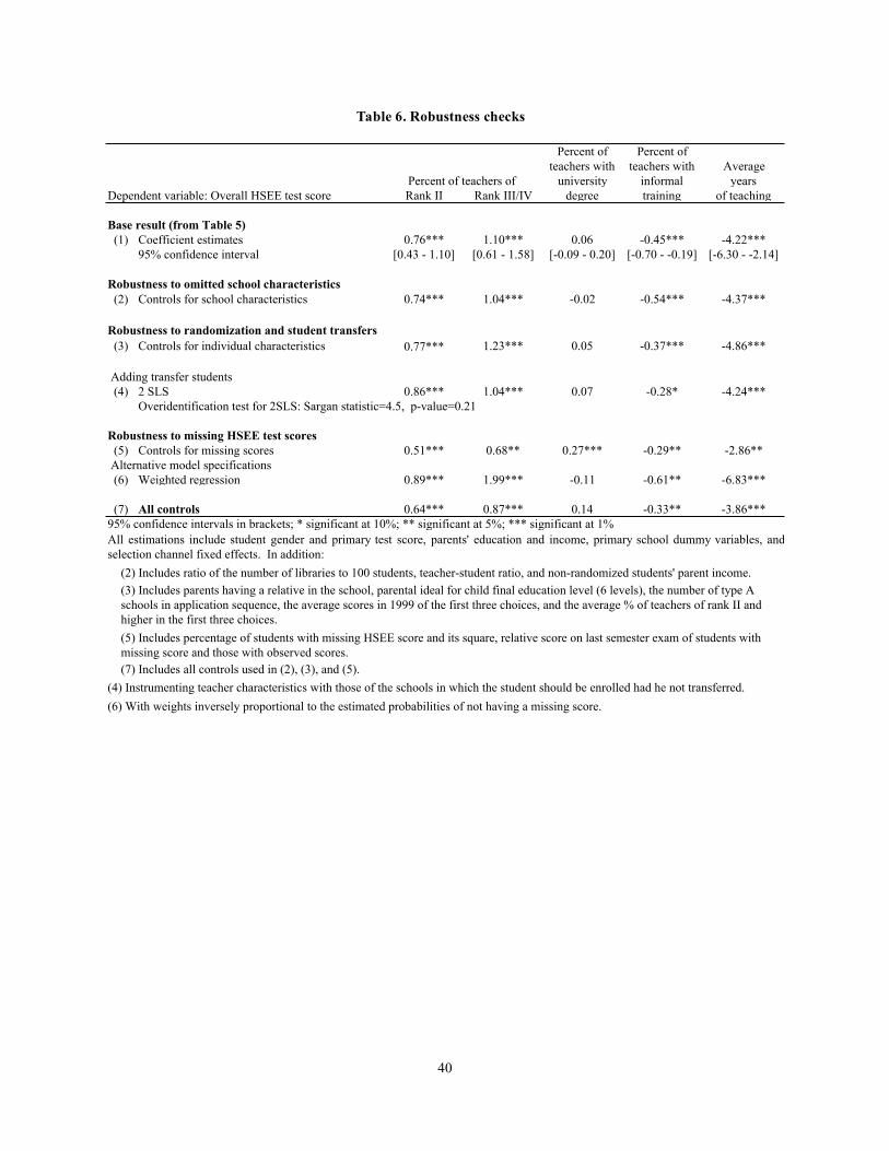
40
Table 6. Robustness checks
Percent of Percent of
teachers with teachers with Average
university informal years
Dependent variable: Overall HSEE test score Rank II Rank III/IV degree training of teaching
Base result (from Table 5)
(1) Coefficient estimates 0.76*** 1.10*** 0.06 -0.45*** -4.22***
95% confidence interval [0.43 - 1.10] [0.61 - 1.58] [-0.09 - 0.20] [-0.70 - -0.19] [-6.30 - -2.14]
Robustness to omitted school characteristics
(2) Controls for school characteristics 0.74*** 1.04*** -0.02 -0.54*** -4.37***
Robustness to randomization and student transfers
(3) Controls for individual characteristics 0.77*** 1.23*** 0.05 -0.37*** -4.86***
Adding transfer students
(4) 2 SLS 0.86*** 1.04*** 0.07 -0.28* -4.24***
Overidentification test for 2SLS: Sargan statistic=4.5, p-value=0.21
Robustness to missing HSEE test scores
(5) Controls for missing scores 0.51*** 0.68** 0.27*** -0.29** -2.86**
Alternative model specifications
(6) Weighted regression 0.89*** 1.99*** -0.11 -0.61** -6.83***
(7) All controls 0.64*** 0.87*** 0.14 -0.33** -3.86***
(7) Includes all controls used in (2), (3), and (5).
(4) Instrumenting teacher characteristics with those of the schools in which the student should be enrolled had he not transferred.
(6) With weights inversely proportional to the estimated probabilities of not having a missing score.
All estimations include student gender and primary test score, parents' education and income, primary school dummy variables, and
selection channel fixed effects. In addition:
(2) Includes ratio of the number of libraries to 100 students, teacher-student ratio, and non-randomized students' parent income.
(3) Includes parents having a relative in the school, parental ideal for child final education level (6 levels), the number of type A
schools in application sequence, the average scores in 1999 of the first three choices, and the average % of teachers of rank II and
higher in the first three choices.
(5) Includes percentage of students with missing HSEE score and its square, relative score on last semester exam of students with
missing score and those with observed scores.
Percent of teachers of
95% confidence intervals in brackets; * significant at 10%; ** significant at 5%; *** significant at 1%