The Contribution of Economic Datato Bank-Failure Models

Working Paper 2003-03August 2003

Daniel A. Nuxoll∗

∗ This working paper reports the details of one part of a three-part study done in close collaboration with JohnO’Keefe and Katherine Samolyk. See Nuxoll, O’Keefe, and Samolyk (2003). While each author had primaryresponsibility for one part of that study, many of the ideas in this part were developed in close collaboration withO’Keefe and Samolyk.

The opinions expressed here are the author’s and do not necessarily reflect the views of the FDIC.

1

Abstract

The wave of bank failures during the late 1980s and early 1990s was caused in part by a

series of regional recessions. This paper examines whether the FDIC can use state-level

economic data to forecast bank failures and finds that these data do not improve models

that use only bank-level data. The paper also proposes a number of explanations for the

lack of improvement.

2

Virtually all economists would accept that economic conditions affect the health

of banks. An FDIC research team has investigated whether this basic theory can be

translated into a forecasting model, and specifically whether nonbank economic data can

be used to improve forecasts of bank health. This project was a systematic effort to

explore the somewhat surprising result noted by some of the developers of the Federal

Reserve System’s off-site program: regional economic variables do not improve the

forecasts of bank health. 1

This paper reports on one aspect of that project: whether nonbank data can

improve bank-failure forecasts.2 In general, we find that economic data do not improve

these forecasts despite the fact that the data are statistically significant.3 Possible

explanations for this result are explored in the conclusion.

This paper begins with a short description of the relationship between bank

conditions and economic events in several regions in the United States. The second

section describes both the bank-specific and the economic data used in this exercise. The

third discusses bank-failure models in general before turning to whether economic data

improve failure models. The conclusion speculates about the possible reasons that state-

level economic data do not improve the forecasts.

1 See Cole, Cornyn, and Gunther (1995), 8.

2 For the purposes of this paper, bank failures include banks that are resolved by the FDIC and cases of open-bankassistance.

3 It is impossible to demonstrate conclusively that including economic data in forecasting models is futile. A vastnumber of models are conceivable, so anyone who really believes in the usefulness of economic data would argue thatthe problem is that the wrong model has been tested. The failure of one model, or even of numerous models, does notnecessarily reflect on all models. Obviously, this observation applies to any negative empirical finding. Nonetheless,the negative finding of this paper, despite extensive specification searching, must raise questions about any futureforecasting exercise that does successfully use economic data. In particular, one must ask whether the success is due tothe power of the model or is the result of a lucky data-mining expedition.

3

Bank Conditions and Economic Events

A casual examination of data from the past couple of decades might suggest that

there is a very weak connection between the health of the economy and the health of the

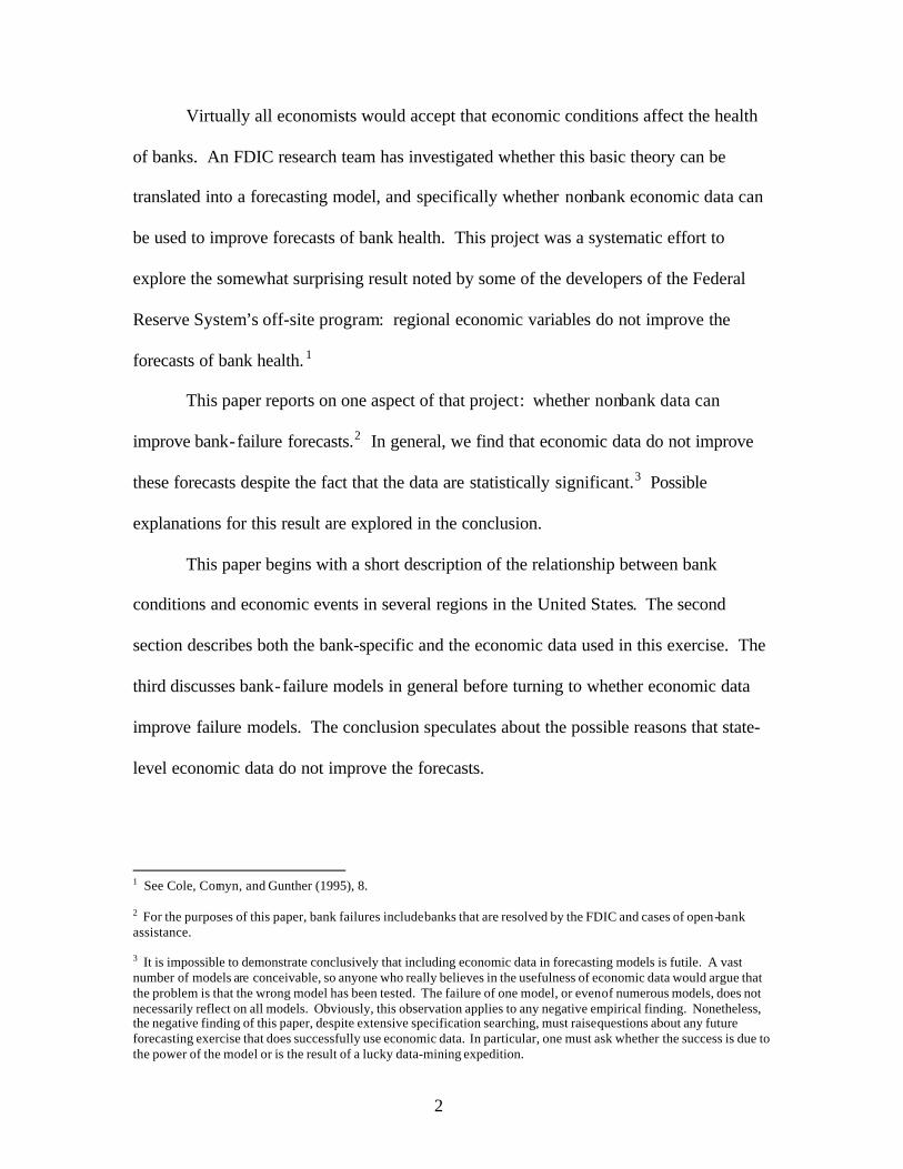
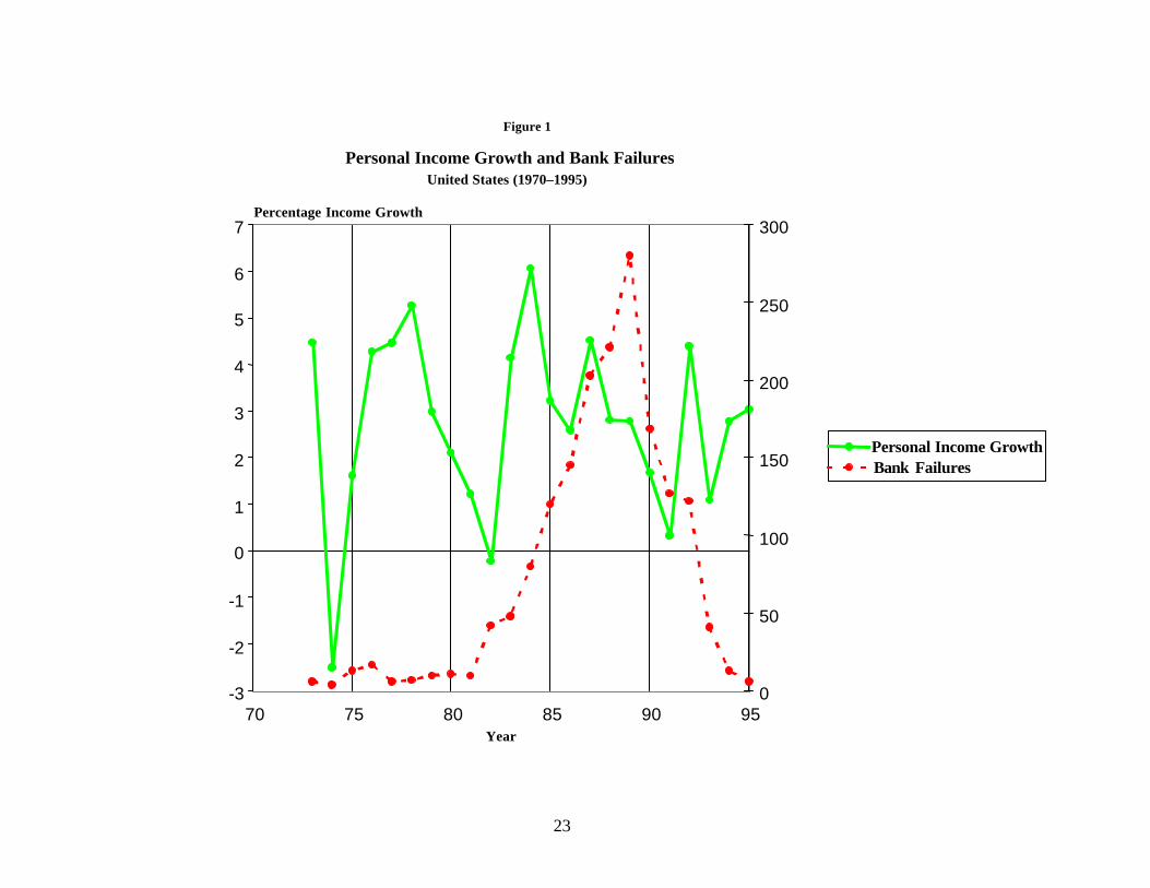
banking sector. Figure 1 plots the growth rate of personal income (solid line) in the

United States as well as the number of bank failures (broken line). The number of

failures did increase shortly after the recessions of 1973 and 1980–1982. However,

failures actually peaked in 1989, following a period of steady economic growth. During

the recession of 1991–1992, fewer banks failed than in preceding years

However, most accounts that stress the importance of the economy to the banking

industry stress the importance of local economies. The FDIC’s History of the Eighties

(1997) refers extensively to local economic conditions in its discussions of the difficulties

experienced by agricultural banks and of banking problems in the Southwest, New

England, and California. Until the 1980s, many states severely limited the geographic

market for banks by legally restricting branching and bank holding companies.

Consequently, almost all banks tended to draw all their deposits from their home states

and to make the bulk of their loans in a very circumscribed area. The relevant economic

conditions for most banks were local, not national.

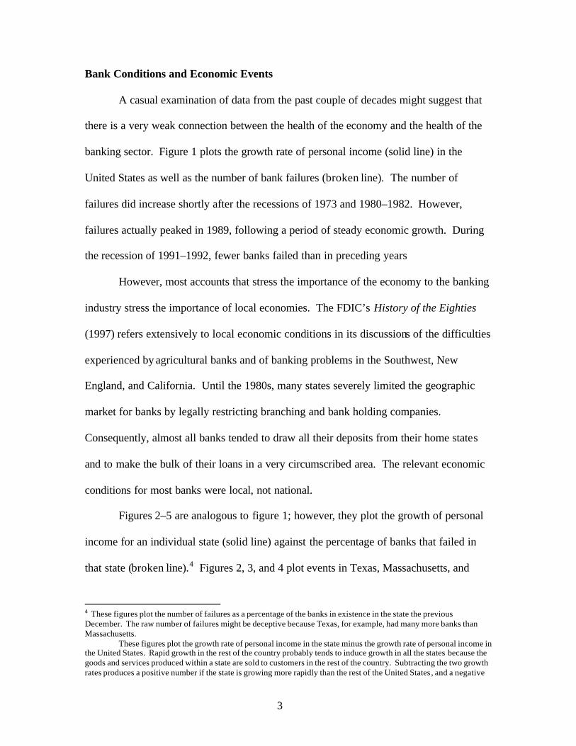
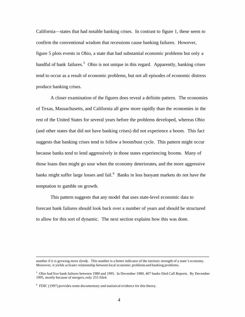
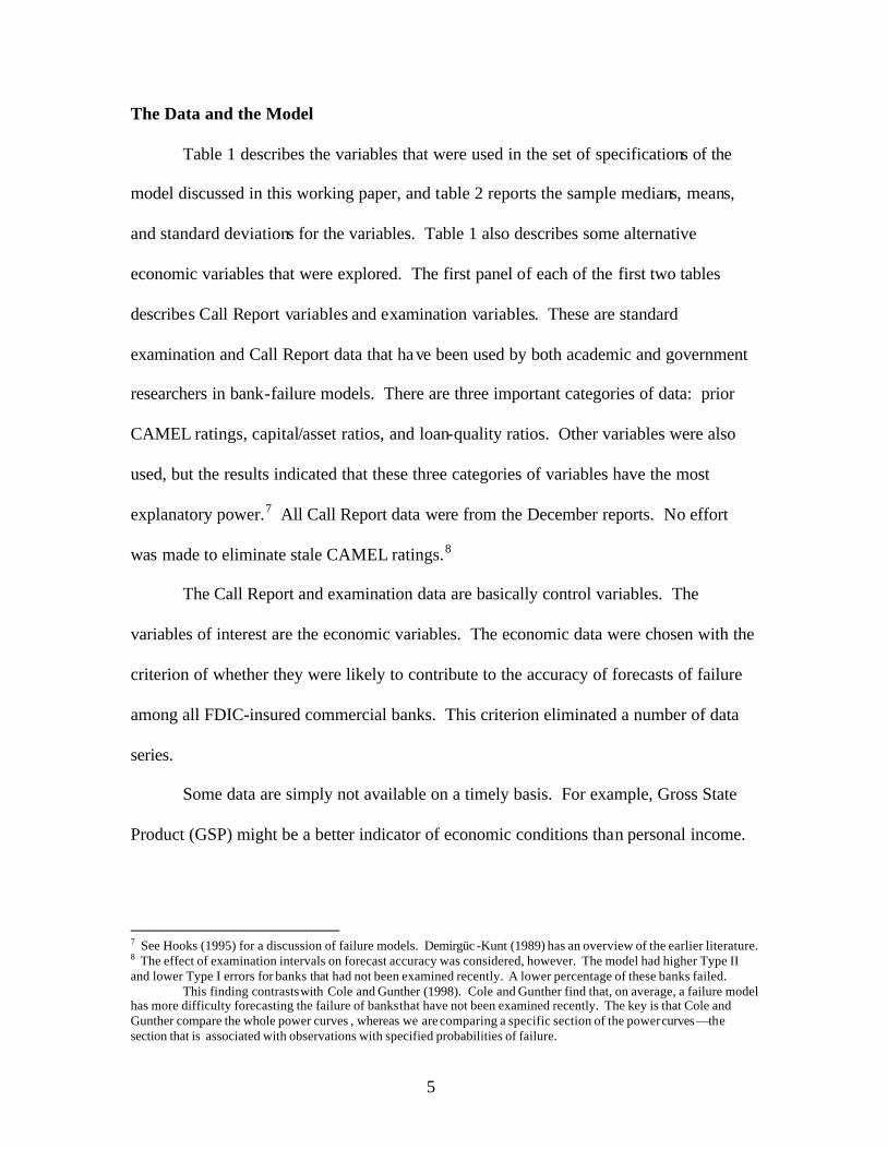
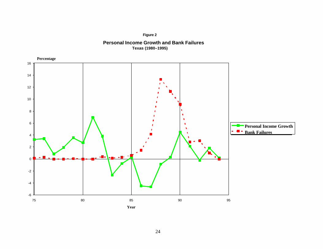
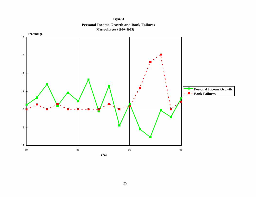
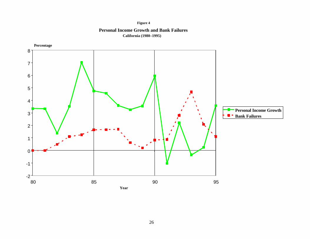
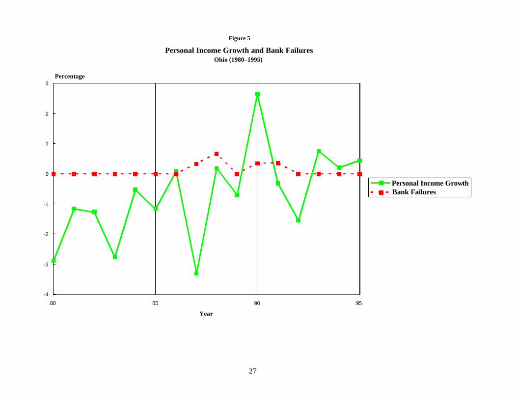
Figures 2–5 are analogous to figure 1; however, they plot the growth of personal

income for an individual state (solid line) against the percentage of banks that failed in

that state (broken line).4 Figures 2, 3, and 4 plot events in Texas, Massachusetts, and

4 These figures plot the number of failures as a percentage of the banks in existence in the state the previousDecember. The raw number of failures might be deceptive because Texas, for example, had many more banks thanMassachusetts.

These figures plot the growth rate of personal income in the state minus the growth rate of personal income inthe United States. Rapid growth in the rest of the country probably tends to induce growth in all the states because thegoods and services produced within a state are sold to customers in the rest of the country. Subtracting the two growthrates produces a positive number if the state is growing more rapidly than the rest of the United States, and a negative

4

California—states that had notable banking crises. In contrast to figure 1, these seem to

confirm the conventional wisdom that recessions cause banking failures. However,

figure 5 plots events in Ohio, a state that had substantial economic problems but only a

handful of bank failures.5 Ohio is not unique in this regard. Apparently, banking crises

tend to occur as a result of economic problems, but not all episodes of economic distress

produce banking crises.

A closer examination of the figures does reveal a definite pattern. The economies

of Texas, Massachusetts, and California all grew more rapidly than the economies in the

rest of the United States for several years before the problems developed, whereas Ohio

(and other states that did not have banking crises) did not experience a boom. This fact

suggests that banking crises tend to follow a boom/bust cycle. This pattern might occur

because banks tend to lend aggressively in those states experiencing booms. Many of

those loans then might go sour when the economy deteriorates, and the more aggressive

banks might suffer large losses and fail.6 Banks in less buoyant markets do not have the

temptation to gamble on growth.

This pattern suggests that any model that uses state-level economic data to

forecast bank failures should look back over a number of years and should be structured

to allow for this sort of dynamic. The next section explains how this was done.

number if it is growing more slowly. This number is a better indicator of the intrinsic strength of a state’s economy.Moreover, it yields a clearer relationship between local economic problems and banking problems.

5 Ohio had five bank failures between 1980 and 1995. In December 1980, 407 banks filed Call Reports. By December1995, mostly because of mergers, only 255 filed.

6 FDIC (1997) provides some documentary and statistical evidence for this theory.

5

The Data and the Model

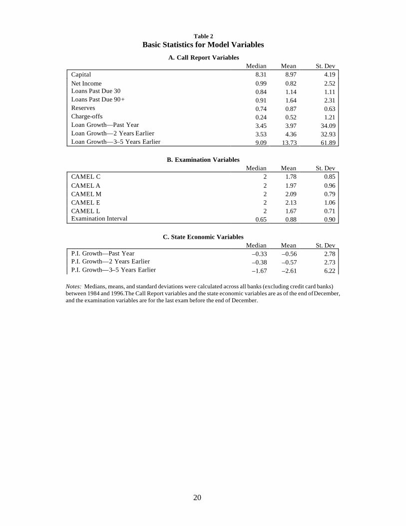
Table 1 describes the variables that were used in the set of specifications of the

model discussed in this working paper, and table 2 reports the sample medians, means,

and standard deviations for the variables. Table 1 also describes some alternative

economic variables that were explored. The first panel of each of the first two tables

describes Call Report variables and examination variables. These are standard

examination and Call Report data that have been used by both academic and government

researchers in bank-failure models. There are three important categories of data: prior

CAMEL ratings, capital/asset ratios, and loan-quality ratios. Other variables were also

used, but the results indicated that these three categories of variables have the most

explanatory power.7 All Call Report data were from the December reports. No effort

was made to eliminate stale CAMEL ratings.8

The Call Report and examination data are basically control variables. The

variables of interest are the economic variables. The economic data were chosen with the

criterion of whether they were likely to contribute to the accuracy of forecasts of failure

among all FDIC-insured commercial banks. This criterion eliminated a number of data

series.

Some data are simply not available on a timely basis. For example, Gross State

Product (GSP) might be a better indicator of economic conditions than personal income.

7 See Hooks (1995) for a discussion of failure models. Demirgüc -Kunt (1989) has an overview of the earlier literature.8 The effect of examination intervals on forecast accuracy was considered, however. The model had higher Type IIand lower Type I errors for banks that had not been examined recently. A lower percentage of these banks failed.

This finding contrasts with Cole and Gunther (1998). Cole and Gunther find that, on average, a failure modelhas more difficulty forecasting the failure of banks that have not been examined recently. The key is that Cole andGunther compare the whole power curves , whereas we are comparing a specific section of the power curves —thesection that is associated with observations with specified probabilities of failure.

6

However, GSP data are available only with a lag of a couple of years, so 1998 data might

be available only in 2000.

Second, the data must exist for times and locations in which there were a

substantial number of bank failures. For example, even with the best data one could

probably not estimate any sort of reasonable bank-failure model for the states of

Alabama, Georgia, Mississippi, North Carolina, and South Carolina. These five states

had a total of 18 bank failures between 1980 and 1995, and there are simply not enough

observations to estimate accurately any kind of model. Similarly, there was one bank

failure in 1997 in the whole United States, so it is impossible to estimate any reasonable

bank-failure model based solely on the data for that year.

Finally, other data are available for some regions but not for all. These data are

potentially useful only for a subset of FDIC-insured banks; but this project had a broader

focus. For example, a wide variety of series on local economic conditions are available

only for a few states or cities. Forecasts of regional economic conditions might be a very

useful indicator of the likelihood that banks in a region will fail in the future. Many firms

produce those forecasts for some states or cities. However, the coverage of these

forecasts is spotty, so their usefulness is limited.

Three broad categories of data meet the basic criterion: personal- income data,

employment data, and banking aggregates.9 Table 1 lists a number of these data series as

“State Economic Variables” or “Alternative State Economic Variables.” During the

course of this project, each of these data series was tested. In general, the employment

9 All dollar-denominated numbers were deflated to 1992, though deflation makes no difference except in thespecifications that pool the data for different periods.

7

data were the least useful, and growth in personal income and growth in total loans made

by banks headquartered in a state improved the failure models the most.

In order to include the type of dynamic discussed above, we used five years’

worth of data in the models. For example, if the growth rate in personal income was

used, the model included five growth-rate terms—the rates from the year before the Call

Report, from two years before it, and from three, four, and five years before it. Some

experimentation revealed that using five years of data produced coefficients that were

imprecisely estimated. The data are highly correlated, so the model cannot distinguish

the effects of growth five years earlier from the effects of growth three years earlier. For

that reason, most work used the growth rate of personal income between three and five

years earlier, the growth rate two years earlier, and the previous year’s growth rate.10

This approach produced more precise coefficient estimates and better forecasts.

Throughout this project, a logistic model was used. This is a standard model

among both academics and bank regulators.11 The model was fitted on bank failures that

occurred within two years of the Call Report date, so the model can be said to have a

two-year horizon.

After the model was fitted, out-of-sample forecasts were done. Because of the

two-year horizon, the forecasts were based on data from the Call Report two years after

the Call Report used to fit the model. For example, the model was fitted on failures in

1990 and 1991, Call Report data from December 1989, and the CAMEL rating for the

10 As in figures 2–5, the personal-income growth rate actually used is the difference between the personal-incomegrowth rate in the state and the rate in the nation.

Table 2 reports an apparently puzzling result : the mean and median growth rates are negative. However,these numbers are weighted by the number of banks in each state. The negative number means that the states with alarge number of banks grew more slowly than the rest of the country.11 The Federal Reserve System has, for several years, used an off-site system that includes a logistic model to forecastbank strength.

8

last exam before December 1989. The coefficients were then used with Call Report and

examination data from December 1991 to forecast failures in 1992 and 1993. In

principle, the necessary data would have been available at the end of 1991 to forecast the

failures over the next two years.12 This exercise mimics the way the FDIC or other

banking agency might use such a model.

This model was estimated both as a cross section and as a pooled time-series cross

section. This paper reports on the cross-section models estimated on data from the Call

Reports of December 1986, December 1989, and December 1992 as well as on a pooled

time-series cross-section model.13 These results are broadly representative of a much

wider group of results.

These models have two types of errors, conventionally called Type I and Type II

errors. Type I errors occur when the model indicates that a bank will survive, but the

bank does not survive. Type II errors occur when the model predicts that a bank will fail,

but it actually survives. More colloquially, Type I errors occur when the model frees the

guilty, and the Type II errors occur when the model convicts the innocent.14

These models do not produce an unambiguous prediction that a bank will fail;

rather, they estimate the probability that a bank will fail. A bank is projected to fail if its

12 In reality, the Call Report data and the examination data are available with a lag, so the data would have beenavailable in early 1992.

13 The December 1986 cross section, for example, used Call Report data from that date as well as data from the lastexamination before December 1986 and failures from the years 1987 and 1988.

Because of the two-year horizon, there is both an “even” and an “odd” version of the pooled model (theformer uses Call Report data from even-numbered years, the latter from odd-numbered years). Both forms were tested,and there were no material differences. This paper reports the even version.

14 The terminology of Type I and Type II errors is adopted from hypothesis testing. Simpler criteria for forecasts canbe developed. Such criteria, however, would necessarily involve some system of weighting the two types of error. Forinstance, there are criteria involving rank-order statistics, but these can be interpreted as assigning an equal weight tothe two errors. In bank-failure models, Type I errors are usually thought more serious, but there is no generalagreement about the appropriate weights.

9

estimated probability exceeds a specific threshold level. Raising the threshold

necessarily decreases the number of projected failures. Decreasing the number of

projected failures also reduces the number of failures accurately forecasted, as well as the

number of surviving banks projected to fail. Thus, a higher threshold increases the level

of Type I errors and decreases the level of Type II errors. One can easily graph the trade-

off between Type I and Type II errors by varying the threshold.

These graphs can be used to compare the accuracy of various models. More

accurate models have a lower level of Type I errors for any given level of Type II errors.

That is, the curve representing a more accurate model lies below and to the left of the

curve for a less accurate model; or equivalently, the curve lies closer to the origin (which

represents no Type I errors and no Type II errors).

It should be noted that such curves can intersect. In these cases, one model is not

unambiguously better than the other.15

These errors can be measured both in-sample and out-of-sample. In-sample

graphs use the same data that were used to estimate the model, so they reflect the fit of

the data. However, for FDIC purposes, the critical criterion is not statistical fit but

forecasting power. Forecasting is by definition out-of-sample, so out-of-sample errors

are more relevant to the model’s usefulness to the FDIC.

For example, the model was estimated on failures in 1990 and 1991, Call Report

data from December 1989, and the CAMEL rating for the last exam before December

15 Actually, bank supervisors are most interested in the section of the curve that represents a low level of Type IIerrors. Bank supervisors have limited resources to devote to monitoring banks intensively. Failure models and otheroff-site models can be used to identify those banks that are in the most danger of failing so that supervisors can allocatethose resources. Type II errors amount to a waste of resources because supervisory resources are diverted to banks thatare not in danger of failure. Because of the constraint, supervisors are undoubtedly most interested in not wastingresources, that is, in low Type II errors. Consequently, they would be most interested in whether, for low levels of

10

1989. Type I and Type II errors are calculated in terms of the ability of the model to

correctly identify failures in 1990 and 1991—that is, in terms of the data used to estimate

the model. The forecasting exercise uses the coefficients of this same model and

December 1991 data to forecast failures in 1992 and 1993. Because the model was

developed without data from 1992 or 1993, the Type I and Type II errors of this exercise

are more indicative of the usefulness of the model. 16

Results

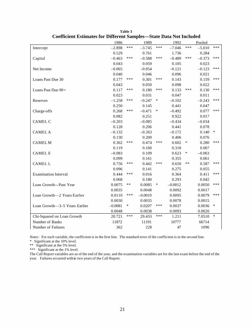
Table 3 reports results for four different samples. The first column gives the

coefficient estimates and standard errors when December 1986 data are used to estimate

the probability of failures in 1987 and 1988. A positive coefficient means that higher

levels of the variable are associated with a larger probability of failure. One asterisk

indicates that the coefficient is significant at least at the 10 percent level, two indicate 5

percent, and three indicate 1 percent. The chi-squared statistic is for the null hypothesis

that all three loan/growth coefficients are zero. The three asterisks indicate that the null

can be rejected at the 1 percent level of significance.

The second and third columns give the results of using December 1989 and

December 1992 data to forecast failures in the following two years. The final column

gives pooled results in which December 1984 data are used to forecast failures in 1985

and 1986, December 1986 data are used to forecast failures in 1987 and 1988, and so

Type II errors , one model has better levels of Type I errors than another. Bank supervisors are relatively uninterestedin whether two curves intersect at high levels of Type II errors .

16 Forecasts for the pooled model were done using a “rolling” system of estimation. For forecasts based on theDecember 1991 Call Report, the pooled model was estimated on data for the period before that date. For December1993 forecasts, two years of data were used to develop the model.

11

forth. The failures in this pooled data set occurred between 1985 and 1996; this period

includes the vast majority of failures of institutions insured by the FDIC.

The results generally indicate that banks with lower levels of capital, higher levels

of past-due loans, and lower loan- loss reserves are more likely to fail. These results are

completely consistent with conventional wisdom and previous studies. Other results have

not been as thoroughly documented, but they are consistent with what one might expect.

Banks with worse CAMEL management and liquidity ratings are also more likely to

fail.17 In addition, banks that have not been examined recently are more likely to fail.

Low income is not a consistently significant indicator of failure, but at least the sign on

net income is consistently negative.

The capital, asset, and earnings CAMEL ratings are mostly statistically

insignificant, and their coefficients are often the “wrong” sign. One possible explanation

is that the capital/asset ratio as well as the loss/reserves ratio conveys the relevant

information in the capital rating, whereas the two past-due loan terms are redundant with

the asset rating, and the earnings rating adds nothing to the net- income term. There are

no variables in this specification that are obvious measures of management quality or

liquidity.

The charge-off/bad loans ratio changes sign, and in the pooled model there is a

statistically significant relationship between high charge-offs and failure. One could

argue either that high charge-offs indicate that the bank has problems in the loan portfolio

(and is likely to fail) or that the bank is dealing with the problems in the portfolio (and is

likely to survive). The statistical results do not differentiate between these two theories.

17 A CAMEL rating of 5 is worse than a CAMEL rating of 1.

12

Finally, there is an ambiguous but generally statistically significant relationship

between a bank’s loan growth and its probability of failure. Small variations in loan

growth are not economically significant, however, because the coefficients are very

small. For example, in the pooled regression, consistent loan growth of 18 percent per

year has about the same effect as a 1 percent difference in the capital/asset ratio.18

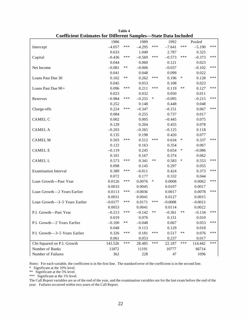
Table 4 reports the results of including the state- level economic data. The chi-

squared statistic is for the null hypothesis that the coefficients on the state data all equal

zero. The results in this table are representative in that the state data are usually highly

significant. If the chi-squared statistic exceed 12.84, the variables are significant at least

at the 5 percent level. The statistics in table 4 exceed this standard by a wide margin.

This result is not quite universal; there are some specifications in which state data are

insignificant in the early 1990s.

The economic data have the expected signs. The negative coefficient on the

previous year’s personal- income growth means that failure is more likely when the state

in which the bank is headquartered is growing less rapidly than the rest of the United

States. The positive coefficient on the growth that occurred between three and five years

earlier means that high growth in the past tends to put banks at more risk. The data

confirm the impression of a boom/bust pattern to bank failures.

Moreover, the coefficients are economically significant. The effect of a 1 percent

decrease in the capital-asset ratio has about the same effect as being located in a state that

18 Mathematically, (–1%) * (–0.373) = 18% * (0.0050 + 0.0079 + 0.0036). This general result is robust across samplesand specifications. This does not translate directly into a probability of failure because the logistic is nonlinear.

This result might seem to contradict previous research that indicates that high growth is a high-risk strategy, atheory that found its way into the provisions of FDICIA. However, the specification includes past-due loans and islimited to a two-year horizon. Possibly, within two years of failure, the quality of the loan portfolio already reflects thenegative effects of high growth. If that is true, then within two years of failure, loans past due (which resulted fromrapid past growth) are a better indicator than the growth itself.

13

was growing 1.4 percent more rapidly than the rest of the nation and is now growing 1.4

percent less rapidly. 19

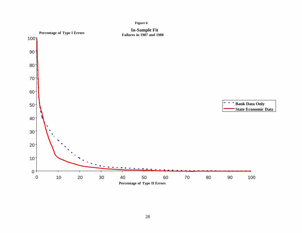
Figure 6 shows the in-sample trade-off between Type I and Type II errors for the

Call Report data from December 1986. The broken line graphs the trade-off between

Type I and Type II errors for the model that uses only bank data, while the solid line

shows the trade-off for the model that includes state economic data. The inclusion of

state data clearly improves the model. The model without state data can achieve a 10

percent Type II error (about 1,200 banks incorrectly considered probable failures) only at

the cost of a 23.2 percent Type I error (84 missed failures). The model with state data

can attain a 10 percent Type II error with only a 10.2 percent Type I error (37 missed

failures). These results are not too surprising because the chi-squared statistic in table 4

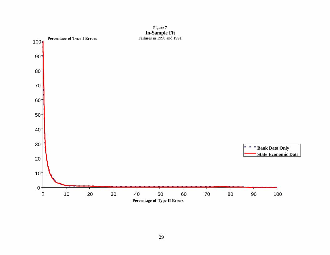
indicates that the state data considerably improve the fit of the model. Figure 7 shows

analogous results for the December 1989 Call Reports. The two curves actually intersect

in this case. Though the state data are statistically significant, there is no obvious

advantage to using the additional data in this period.

Though a model with more data necessarily has at least as good a fit as models

with less data, the same is not true for forecasting. It is well known among

macroeconomic forecasters that more sophisticated models often perform worse than

simpler models.

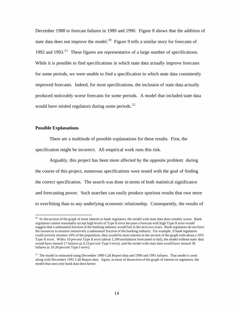
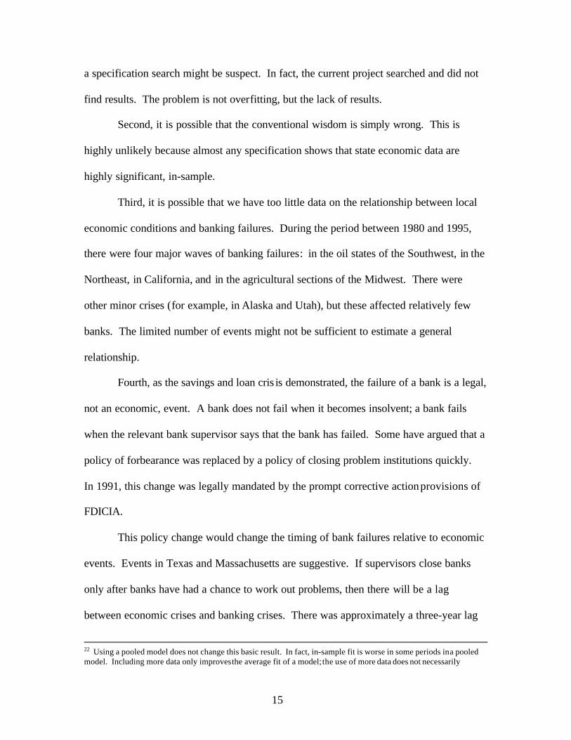
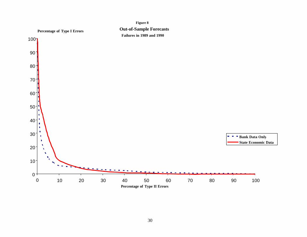
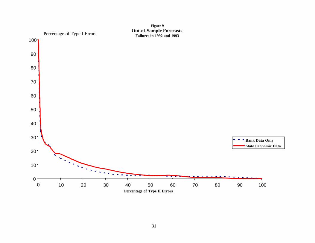
Figures 8 and 9 show the results of two forecasting exercises. Figure 8 shows the

results of using the model estimated on December 1986 Call Report data to estimate the

probability of failure in 1987 and 1988. In principle, an economist could have estimated

this model in January 1989 and used the coefficients and Call Report data from

19 (–1%) * (–0.373) = (–1.4%) * (–.134) + 1.4% * (0.053 + 0.076)

14

December 1988 to forecast failures in 1989 and 1990. Figure 8 shows that the addition of

state data does not improve the model.20 Figure 9 tells a similar story for forecasts of

1992 and 1993.21 These figures are representative of a large number of specifications.

While it is possible to find specifications in which state data actually improve forecasts

for some periods, we were unable to find a specification in which state data consistently

improved forecasts. Indeed, for most specifications, the inclusion of state data actually

produced noticeably worse forecasts for some periods. A model that included state data

would have misled regulators during some periods.22

Possible Explanations

There are a multitude of possible explanations for these results. First, the

specification might be incorrect. All empirical work runs this risk.

Arguably, this project has been more affected by the opposite problem: during

the course of this project, numerous specifications were tested with the goal of finding

the correct specification. The search was done in terms of both statistical significance

and forecasting power. Such searches can easily produce spurious results that owe more

to overfitting than to any underlying economic relationship. Consequently, the results of

20 In the section of the graph of most interest to bank regulators, the model with state data does notably worse. Bankregulators cannot reasonably accept high levels of Type II error because a forecast with high Type II error wouldsuggest that a substantial fraction of the banking industry would fail in the next two years. Bank regulators do not havethe resources to monitor intensively a substantial fraction of the banking industry. For example, if bank regulatorscould actively monitor 10% of the population, they would be most interest in the section of the graph with about a 10%Type II error. With a 10 percent Type II error (about 1,100 nonfailures forecasted to fail), the model without state datawould have missed 17 failures (a 6.23 percent Type I error), and the model with state data would have missed 28failures (a 10.26 percent Type I error).

21 The model is estimated using December 1989 Call Report data and 1990 and 1991 failures. That model is usedalong with December 1991 Call Report data. Again, in most of the section of the graph of interest to regulators, themodel that uses only bank data does better.

15

a specification search might be suspect. In fact, the current project searched and did not

find results. The problem is not overfitting, but the lack of results.

Second, it is possible that the conventional wisdom is simply wrong. This is

highly unlikely because almost any specification shows that state economic data are

highly significant, in-sample.

Third, it is possible that we have too little data on the relationship between local

economic conditions and banking failures. During the period between 1980 and 1995,

there were four major waves of banking failures: in the oil states of the Southwest, in the

Northeast, in California, and in the agricultural sections of the Midwest. There were

other minor crises (for example, in Alaska and Utah), but these affected relatively few

banks. The limited number of events might not be sufficient to estimate a general

relationship.

Fourth, as the savings and loan cris is demonstrated, the failure of a bank is a legal,

not an economic, event. A bank does not fail when it becomes insolvent; a bank fails

when the relevant bank supervisor says that the bank has failed. Some have argued that a

policy of forbearance was replaced by a policy of closing problem institutions quickly.

In 1991, this change was legally mandated by the prompt corrective action provisions of

FDICIA.

This policy change would change the timing of bank failures relative to economic

events. Events in Texas and Massachusetts are suggestive. If supervisors close banks

only after banks have had a chance to work out problems, then there will be a lag

between economic crises and banking crises. There was approximately a three-year lag

22 Using a pooled model does not change this basic result. In fact, in-sample fit is worse in some periods in a pooledmodel. Including more data only improves the average fit of a model; the use of more data does not necessarily

16

in Texas (c.f. figure 2). However, if supervisors close banks quickly, the lag will be

shorter. Banks in Massachusetts failed soon after that state went into recession; figure 3

shows practically no lag. If this is the case, the forecasting model performs poorly

because the model is looking for the same lag in Massachusetts that it found in Texas.

Fifth, bank data are economic data. Any reasonable model of bank failure

includes a number of variables that reflect the health of the local economy. Loans past

due 30–89 days, for example, are procyclical and seem to be roughly contemporaneous.23

Because bank balance sheets reflect local economic conditions, the question is whether

other economic data, such as personal- income growth, add anything to that information.

Bank data do have one important advantage in failure models. The bank is

affected by the economy in which it does business. And virtually no bank markets

coincide with state boundaries. Most banks have only a few branches and do business in

a relatively small area, so their health depends less on the condition of the state economy

than on whether the local factory shuts down or whether local farmers can survive a

drought. On the other hand, some banks lend out-of-state, exposing part of their portfolio

to events in other states.24 Of course, money-center banks do business throughout the

world, so the less-developed-country crisis is an inherent part of the history of banks

improve the fit in each year.23 There is a weak relationship (a correlation coefficient of –0.233) between loans past due 30–89 days at banksheadquartered in the state and personal-income growth in the state. The relationship is statistically significant and ofthe same order of magnitude as the correlation of either employment growth or the unemployment rate with personal-income growth.

The contemporaneous relationship is strongest, but there are two important caveats. First, thecontemporaneous relationship is between past-due loans at the end of the quarter and income growth during the quarter.The timing problem is inherent in any comparison between stocks and flows. Second, the difference betweencontemporaneous, leading, and lagging correlation coefficients is tiny. The correlation coefficient between incomegrowth and loans past due at the end of the previous quarter is –0.216, and between income growth and loans past dueat the end of next quarter, –0.211.

As one might expect, there is a lagging relationship with loans past due 90+ days and income growth.Credit card banks are omitted from this analysis.

24 Banks lent far from the home state even before interstate banking.

17

during the 1980s. Currently, the federal agencies do know where banks have branches

and how much money has been deposited in those branches. However, even if these data

were completely accurate (and they are probably not), the major risk to banks is loans,

not deposits. Given these problems, it is virtually impossible to measure economic

conditions accurately within a bank’s market.

The bank’s balance sheet, however, indicates economic conditions precisely

within the bank’s market. Of course, that information is noisy because the quality of the

management and other factors affect the balance sheet. Arguably, this is an advantage,

for the question is not the health of the economy where the bank does business but how

the economy affects the bank. That effect depends heavily on the quality of management.

Hence, state economic data might add little to forecasting models because they do

not add any information to the data already in the model.

It must be stressed that these explanations are conjectural. Some are logically

impossible to verify (for example, logically one can never show that there is no additional

information in data). Moreover, the proposed reasons are undoubtedly incomplete.25

Though the reasons for our failure to find an effect are not obvious, it is obvious

that we did not find a way to use state economic data to improve forecasts of bank failure.

25 Most importantly, the surge of failures between 1980 and 1995 was unique in FDIC history. This suggests eitherthat regional recessions did not occur before 1980 (which seems implausible) or that something happened after 1980 tomake banks more susceptible to failure.

18

References

Cole, Rebel A., Barbara G. Cornyn, and Jeffery W. Gunther. 1995. FIMS: A NewMonitoring System for Banking Institutions. Federal Reserve Bulletin 81, no. 1:1–15.

Cole, Rebel A., and Jeffery W. Gunther. 1998. Predicting Bank Failures: A Comparisonof On- and Off-Site Monitoring Systems. Journal of Financial Services Research 13no. 2:103–17.

Demirgüc-Kunt, Asli. 1989. Deposit-Institution Failures: A Review of the EmpiricalLiterature. Federal Reserve Bank of Cleveland Economic Review 25, no. 4:2–18.

Federal Deposit Insurance Corporation (FDIC). 1997. History of the Eighties—Lessonsfor the Future. 2 vols. FDIC.

Hooks, Linda M. 1995. Bank Asset Risk—Evidence from Early Warning Models.Contemporary Economic Policy 13, no. 4:36–50.

Nuxoll, Daniel A., John O’Keefe, and Katherine Samolyk. 2003. Do Local EconomicData Improve Off-Site Models That Monitor Bank Performance? FDIC BankingReview (in press).

19

Table 1

Variables Used in the Failure ModelA. Call Report Variables

Capital Equity as a percentage of total assetsNet Income Net income as a percentage of total assets

Due 30 Loans past due 30–89 days as a percentage of total assetsLoans Past Due 90+ Loans past due 90 or more days plus nonaccruing loans plus other real estate owned (repossessed real estate)

as a percentage of total assetsReserves Loan-loss reserves as a percentage of loans past due 90 days plus nonaccruing loans plus other real estate

ownedCharge-offs

Charge-offs as a percentage of loans past due 90 days plus nonaccruing loans plus other real estate ownedLoan Growth—Past Year

Percentage growth in total loans (deflated by the GDP deflator) between the December Call Report and theDecember Call Report of the previous year

Loan Growth—2 Years Earlier

Percentage growth in total loans (deflated by the GDP deflator) between the December Call Report of theprevious year and the December Call Report of the year before that

Loan Growth—3–5 Years Earlier

Average percentage growth in total loans (deflated by the GDP deflator) between the December Call Report oftwo years earlier and the December Call Report of five years earlier

B. Examination VariablesCAMEL C Capital component of CAMEL ratingCAMEL A Asset component of CAMEL ratingCAMEL M Management component of CAMEL ratingCAMEL E Earnings component of CAMEL ratingCAMEL L Liquidity component of CAMEL ratingExamination Interval Number of days between the Call Report date and the last examination, divided by 365

C. State Economic VariablesP.I. Growth—Past Year

Percentage growth in total personal income during the past year minus the comparable number for the UnitedStates

P.I. Growth—2 Years Earlier Percentage growth in total personal income two years ago minus the comparable number for the United StatesP.I. Growth—3–5 Years Earlier

Average percentage growth in total personal income three to five years ago minus the comparable number forthe United States

D. Alternative State Economic VariablesPer Capita Personal Income GrowthDisposable Personal Income GrowthPer Capita Disposable Personal Income GrowthEmployment GrowthUnemployment RateGrowth in Total Loans reported by all banks headquartered in the stateGrowth in Total Assets reported by all banks headquartered in the state

Notes for alterative state economic variables: Five years of data were used. All variables were run both as levels and as differences from thecomparable U.S. value. All variables were run both as levels and as differences from the comparable U.S. value. All dollar values were deflated bythe GDP deflator. Total loans and assets are from the December Call Report. Thrifts and credit card banks were excluded.

20

Table 2

Basic Statistics for Model Variables

A. Call Report VariablesMedian Mean St. Dev

Capital 8.31 8.97 4.19Net Income 0.99 0.82 2.52Loans Past Due 30 0.84 1.14 1.11Loans Past Due 90+ 0.91 1.64 2.31Reserves 0.74 0.87 0.63Charge-offs 0.24 0.52 1.21Loan Growth—Past Year 3.45 3.97 34.09Loan Growth—2 Years Earlier 3.53 4.36 32.93Loan Growth—3–5 Years Earlier 9.09 13.73 61.89

B. Examination VariablesMedian Mean St. Dev

CAMEL C 2 1.78 0.85CAMEL A 2 1.97 0.96CAMEL M 2 2.09 0.79CAMEL E 2 2.13 1.06CAMEL L 2 1.67 0.71Examination Interval 0.65 0.88 0.90

C. State Economic VariablesMedian Mean St. Dev

P.I. Growth—Past Year –0.33 –0.56 2.78P.I. Growth—2 Years Earlier –0.38 –0.57 2.73P.I. Growth—3–5 Years Earlier –1.67 –2.61 6.22

Notes: Medians, means, and standard deviations were calculated across all banks (excluding credit card banks)between 1984 and 1996.The Call Report variables and the state economic variables are as of the end of December,and the examination variables are for the last exam before the end of December.

21

Table 3Coefficient Estimates for Different Samples—State Data Not Included

1986 1989 1992 Pooled Intercept –2.898 *** –3.745 *** –7.046 *** –5.010 *** 0.529 0.761 1.736 0.284 Capital –0.463 *** –0.588 *** –0.489 *** –0.373 *** 0.043 0.059 0.105 0.023 Net Income –0.065 –0.054 –0.121 –0.123 *** 0.040 0.046 0.096 0.021 Loans Past Due 30 0.177 *** 0.301 *** 0.143 0.159 *** 0.043 0.050 0.098 0.022 Loans Past Due 90+ 0.117 *** 0.180 *** 0.133 *** 0.130 *** 0.023 0.031 0.047 0.011 Reserves –1.258 *** –0.247 * –0.102 –0.243 *** 0.250 0.145 0.441 0.047 Charge-offs 0.268 *** –0.471 * –0.492 0.077 *** 0.082 0.251 0.922 0.017 CAMEL C –0.203 –0.085 –0.434 –0.034 0.128 0.206 0.441 0.078 CAMEL A –0.132 –0.263 –0.172 0.140 * 0.130 0.200 0.406 0.076 CAMEL M 0.362 *** 0.474 *** 0.602 * 0.280 *** 0.119 0.160 0.318 0.067 CAMEL E –0.083 0.109 0.623 * –0.063 0.099 0.161 0.355 0.061 CAMEL L 0.756 *** 0.442 *** 0.650 ** 0.587 *** 0.096 0.141 0.275 0.055 Examination Interval 0.444 *** 0.016 0.364 0.411 *** 0.068 0.180 0.293 0.042 Loan Growth—Past Year 0.0075 ** 0.0085 * –0.0012 0.0050 *** 0.0035 0.0048 0.0092 0.0017 Loan Growth—2 Years Earlier 0.0110 *** –0.0019 0.0095 0.0079 *** 0.0030 0.0035 0.0078 0.0015 Loan Growth—3–5 Years Earlier –0.0081 * 0.0207 *** 0.0037 0.0036 * 0.0048 0.0038 0.0093 0.0020 Chi-Squared on Loan Growth 20.721 *** 29.433 *** 1.211 7.0510 *Number of Banks 11872 11191 10777 66714 Number of Failures 362 228 47 1096

Notes: For each variable, the coefficient is in the first line. The standard error of the coefficient is in the second line.* Significant at the 10% level.** Significant at the 5% level.*** Significant at the 1% level.The Call Report variables are as of the end of the year, and the examination variables are for the last exam before the end of theyear. Failures occurred within two years of the Call Report.

22

Table 4Coefficient Estimates for Different Samples—State Data Included

1986 1989 1992 Pooled Intercept –4.057 *** –4.295 *** –7.641 *** –5.190 *** 0.633 1.049 2.787 0.325 Capital –0.436 *** –0.569 *** –0.573 *** –0.373 *** 0.044 0.060 0.121 0.023 Net Income –0.081 ** –0.006 –0.037 –0.102 *** 0.041 0.048 0.099 0.022 Loans Past Due 30 0.102 ** 0.262 *** 0.196 * 0.128 *** 0.045 0.053 0.108 0.023 Loans Past Due 90+ 0.096 *** 0.211 *** 0.119 ** 0.127 *** 0.023 0.032 0.050 0.011 Reserves –0.984 *** –0.255 * –0.095 –0.215 *** 0.252 0.148 0.448 0.048 Charge-offs 0.224 *** –0.347 –0.151 0.067 *** 0.084 0.255 0.737 0.017 CAMEL C 0.002 0.005 –0.445 0.075 0.129 0.204 0.455 0.078 CAMEL A –0.203 –0.265 –0.125 0.118 0.135 0.198 0.420 0.077 CAMEL M 0.503 *** 0.512 *** 0.634 * 0.337 *** 0.122 0.163 0.354 0.067 CAMEL E –0.119 0.245 0.654 * –0.086 0.101 0.167 0.374 0.062 CAMEL L 0.573 *** 0.341 ** 0.583 * 0.553 *** 0.098 0.145 0.297 0.055 Examination Interval 0.389 *** –0.011 0.424 0.373 *** 0.072 0.177 0.332 0.044 Loan Growth—Past Year 0.0126 *** 0.0076 * 0.0008 0.0062 *** 0.0033 0.0045 0.0107 0.0017 Loan Growth—2 Years Earlier 0.0113 *** –0.0036 0.0017 0.0078 *** 0.0031 0.0041 0.0127 0.0015 Loan Growth—3–5 Years Earlier –0.0177 *** 0.0171 *** –0.0008 –0.0013 0.0053 0.0041 0.0114 0.0022 P.I. Growth—Past Year –0.213 *** –0.142 ** –0.361 ** –0.134 *** 0.019 0.076 0.151 0.010 P.I. Growth—2 Years Earlier –0.100 ** –0.048 0.067 0.053 *** 0.048 0.113 0.129 0.018 P.I. Growth—3–5 Years Earlier 0.326 *** 0.181 *** 0.517 ** 0.076 *** 0.061 0.053 0.237 0.017 Chi-Squared on P.I. Growth 143.526 *** 28.485 *** 22.187 *** 114.442 ***Number of Banks 11872 11191 10777 66714 Number of Failures 362 228 47 1096

Notes: For each variable, the coefficient is in the first line. The standard error of the coefficient is in the second line.* Significant at the 10% level.** Significant at the 5% level.*** Significant at the 1% level.The Call Report variables are as of the end of the year, and the examination variables are for the last exam before the end of theyear. Failures occurred within two years of the Call Report.

23

Figure 1

Personal Income Growth and Bank FailuresUnited States (1970–1995)

-3

-2

-1

0

1

2

3

4

5

6

7

70 75 80 85 90 95Year

Percentage Income Growth

0

50

100

150

200

250

300

Personal Income GrowthBank Failures

24

Figure 2

Personal Income Growth and Bank FailuresTexas (1980–1995)

-6

-4

-2

0

2

4

6

8

10

12

14

16

75 80 85 90 95

Year

Percentage

Personal Income GrowthBank Failures

25

Figure 3

Personal Income Growth and Bank FailuresMassachusetts (1980–1995)

-4

-2

0

2

4

6

8

80 85 90 95

Year

Percentage

Personal Income GrowthBank Failures

26

Figure 4

Personal Income Growth and Bank FailuresCalifornia (1980–1995)

-2

-1

0

1

2

3

4

5

6

7

8

80 85 90 95Year

Percentage

Personal Income GrowthBank Failures

27

Figure 5

Personal Income Growth and Bank FailuresOhio (1980–1995)

-4

-3

-2

-1

0

1

2

3

80 85 90 95

Year

Percentage

Personal Income GrowthBank Failures

28

Figure 6

In-Sample FitFailures in 1987 and 1988

0

10

20

30

40

50

60

70

80

90

100

0 10 20 30 40 50 60 70 80 90 100Percentage of Type II Errors

Percentage of Type I Errors

Bank Data OnlyState Economic Data

29

0

10

20

30

40

50

60

70

80

90

100

0 10 20 30 40 50 60 70 80 90 100Percentage of Type II Errors

Bank Data OnlyState Economic Data

Percentage of Type I Errors

Figure 7

In-Sample FitFailures in 1990 and 1991

30

Figure 8

Out-of-Sample ForecastsFailures in 1989 and 1990

0

10

20

30

40

50

60

70

80

90

100

0 10 20 30 40 50 60 70 80 90 100Percentage of Type II Errors

Percentage of Type I Errors

Bank Data OnlyState Economic Data

31

0

10

20

30

40

50

60

70

80

90

100

0 10 20 30 40 50 60 70 80 90 100Percentage of Type II Errors

Bank Data OnlyState Economic Data

Figure 9

Out-of-Sample ForecastsFailures in 1992 and 1993Percentage of Type I Errors