The continuous adjoint strikes back

Francisco Palacios

(with results from S. Copeland, T. Economon and A. Pozo PhD thesis)

Department of Aeronautics & Astronautics Stanford University

A J 8 0 T H

S TA N F O R D U N I V E R S I T Y N O V E M B E R 2 1 S T , 2 0 1 4

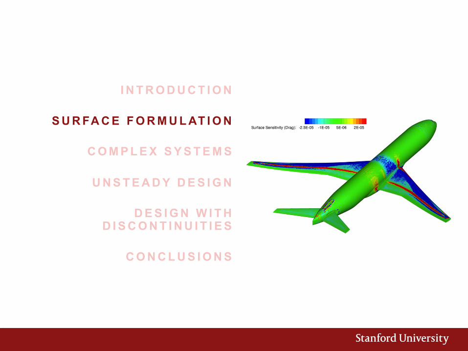
I N T R O D U C T I O N

S U R FA C E F O R M U L AT I O N

C O M P L E X S Y S T E M S

U N S T E A D Y D E S I G N

D E S I G N W I T H D I S C O N T I N U I T I E S

C O N C L U S I O N S

Optimum Aircraft Design

Flexible aircraft

Loads and aeroelastics

Optimum flight control

Structural optimization

Performance optimization

The continuous adjoint strikes back or… the revenge of the continuous adjoint (a personal vision) •  The aerodynamic optimal shape methodology using control theory

was discovered and developed by Prof. Jameson (~100 articles). From theory to complex applications.

•  Prof. Jameson mainly worked on the continuous and the discrete (by hand) adjoint. And, in both cases, he demonstrated that the method was mature to deal with complex wing body configurations.

Then… something happened…

•  The CFD community started looking at the Automatic Differentiation based techniques and we entered in a stall situation where the new “more accurate” techniques were not able to deal with complex problems, putting a brake on the industrial application.

Now... just few industrial CFD adjoint solvers are able to reproduce optimizations done by Prof. Jameson 10-15 years ago… It is time to rediscover the continuous adjoint methodology and exploit its advantages.

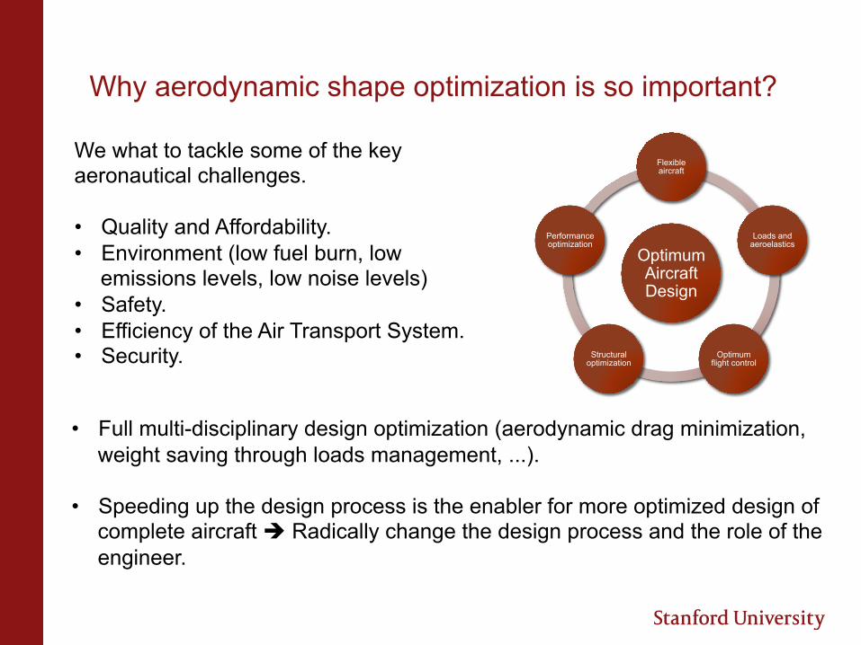
Why aerodynamic shape optimization is so important?

We what to tackle some of the key aeronautical challenges. •  Quality and Affordability. •  Environment (low fuel burn, low

emissions levels, low noise levels) •  Safety. •  Efficiency of the Air Transport System. •  Security.

Optimum Aircraft Design

Flexible aircraft

Loads and aeroelastics

Optimum flight control

Structural optimization

Performance optimization

•  Full multi-disciplinary design optimization (aerodynamic drag minimization,

weight saving through loads management, ...).

•  Speeding up the design process is the enabler for more optimized design of complete aircraft è Radically change the design process and the role of the engineer.

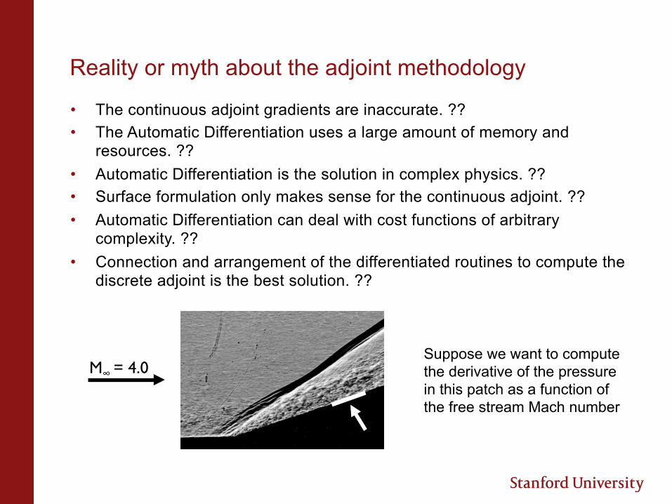
Reality or myth about the adjoint methodology

•  The continuous adjoint gradients are inaccurate. ?? •  The Automatic Differentiation uses a large amount of memory and

resources. ?? •  Automatic Differentiation is the solution in complex physics. ?? •  Surface formulation only makes sense for the continuous adjoint. ?? •  Automatic Differentiation can deal with cost functions of arbitrary

complexity. ?? •  Connection and arrangement of the differentiated routines to compute the

discrete adjoint is the best solution. ??

M∞ = 4.0

Suppose we want to compute the derivative of the pressure in this patch as a function of the free stream Mach number

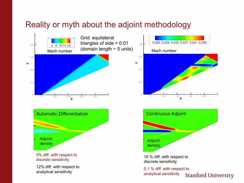
Reality or myth about the adjoint methodology Grid: equilateral triangles of side = 0.01 (domain length ~ 5 units) Mach number Mach number

Automatic Differentiation

0% diff. with respect to discrete sensitivity

12% diff. with respect to analytical sensitivity

Continuous Adjoint

10 % diff. with respect to discrete sensitivity

0.1 % diff. with respect to analytical sensitivity

Adjoint density

Adjoint density

In this talk

•  The objective of this talk is to present an overview of challenges and opportunities for the continuous adjoint methodology.

•  Highlighting those areas in which the continuous adjoint makes a difference from the industrial point of view:

-  Fully exploit the surface formulation, understand the limitations and advantages.

-  Complex systems, more complex equations, more complex geometries, larger problems.

-  Efficient unsteady design. -  Design with discontinuities.

I N T R O D U C T I O N

S U R FA C E F O R M U L AT I O N

C O M P L E X S Y S T E M S

U N S T E A D Y D E S I G N

D E S I G N W I T H D I S C O N T I N U I T I E S

C O N C L U S I O N S

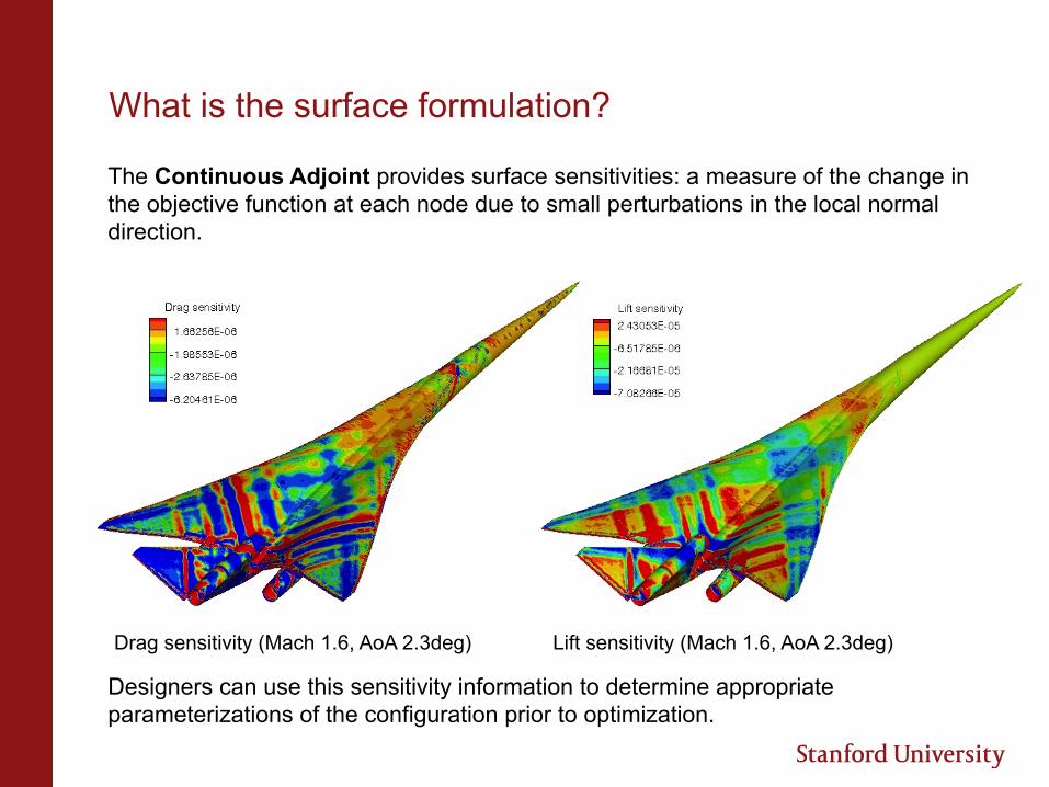
Designers can use this sensitivity information to determine appropriate parameterizations of the configuration prior to optimization.

Drag sensitivity (Mach 1.6, AoA 2.3deg) Lift sensitivity (Mach 1.6, AoA 2.3deg)

What is the surface formulation?

The Continuous Adjoint provides surface sensitivities: a measure of the change in the objective function at each node due to small perturbations in the local normal direction.

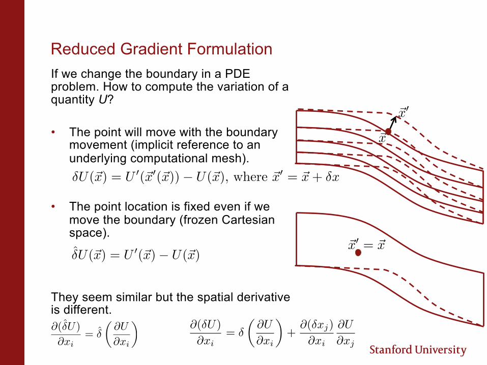
Reduced Gradient Formulation If we change the boundary in a PDE problem. How to compute the variation of a quantity U? •  The point will move with the boundary

movement (implicit reference to an underlying computational mesh).

•  The point location is fixed even if we move the boundary (frozen Cartesian space).

They seem similar but the spatial derivative is different.

�U(~x) = U

0(~x0(~x))� U(~x), where ~x

0 = ~x+ �x

�̂U(~x) = U

0(~x)� U(~x)

@(�̂U)

@xi= �̂

✓@U

@xi

◆@(�U)

@xi= �

✓@U

@xi

◆+

@(�xj)

@xi

@U

@xj

�U(~x) = U

0(~x0(~x))� U(~x), where ~x

0 = ~x+ �x

�U(~x) = U

0(~x0(~x))� U(~x), where ~x

0 = ~x+ �x

�U(~x) = U

0(~x0(~x))� U(~x), where ~x

0 = ~x+ �x

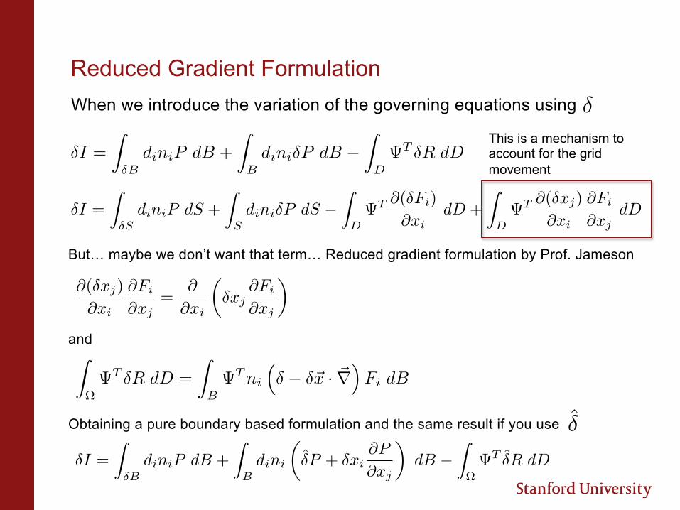
Reduced Gradient Formulation When we introduce the variation of the governing equations using

�

�I =

Z

�SdiniP dS +

Z

Sdini�P dS �

Z

D T @(�Fi)

@xidD +

Z

D T @(�xj)

@xi

@Fi

@xjdD

�I =

Z

�BdiniP dB +

Z

Bdini�P dB �

Z

D T �R dD

This is a mechanism to account for the grid movement

But… maybe we don’t want that term… Reduced gradient formulation by Prof. Jameson and Obtaining a pure boundary based formulation and the same result if you use

@(�xj)

@xi

@Fi

@xj=

@

@xi

✓�xj

@Fi

@xj

◆

Z

⌦ T

�R dD =

Z

B T

ni

⇣� � �~x · ~r

⌘Fi dB

�̂

�I =

Z

�BdiniP dB +

Z

Bdini

✓�̂P + �xi

@P

@xj

◆dB �

Z

⌦ T

�̂R dD

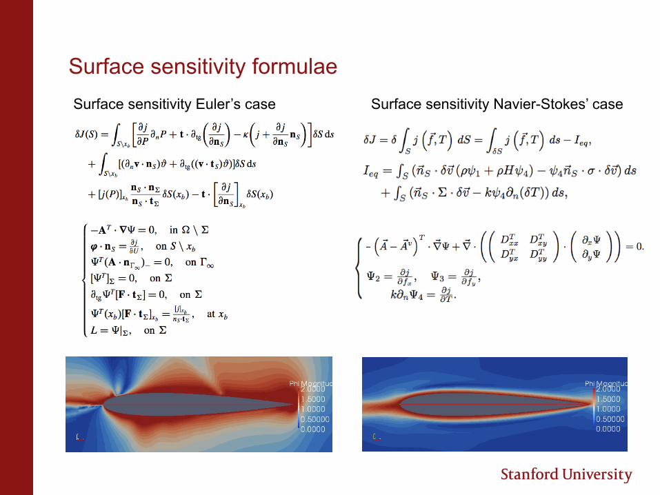
Surface sensitivity formulae Surface sensitivity Navier-Stokes’ case Surface sensitivity Euler’s case

I N T R O D U C T I O N

S U R FA C E F O R M U L AT I O N

C O M P L E X S Y S T E M S

U N S T E A D Y D E S I G N

D E S I G N W I T H D I S C O N T I N U I T I E S

C O N C L U S I O N S

Image | UCI Flight Dynamics & Control Lab

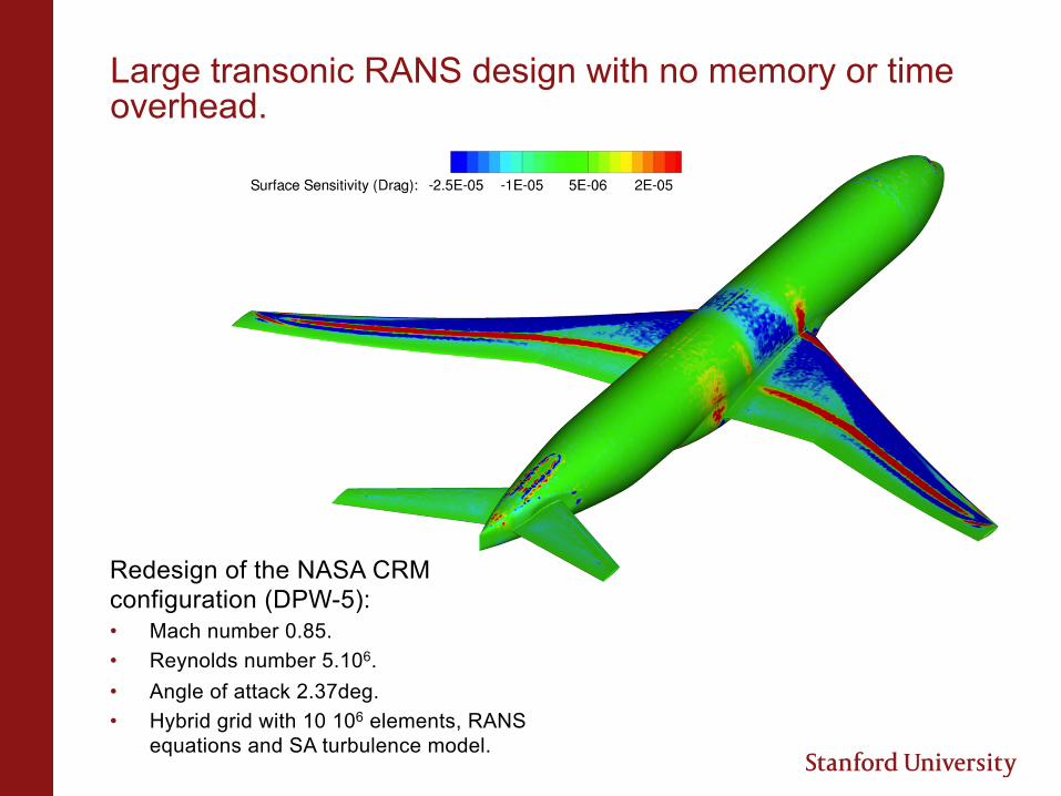
Redesign of the NASA CRM configuration (DPW-5): •  Mach number 0.85. •  Reynolds number 5.106. •  Angle of attack 2.37deg. •  Hybrid grid with 10 106 elements, RANS

equations and SA turbulence model.

Large transonic RANS design with no memory or time overhead.

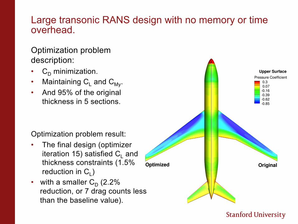
Optimization problem description: •  CD minimization. •  Maintaining CL and CMy. •  And 95% of the original

thickness in 5 sections.

Optimization problem result: •  The final design (optimizer

iteration 15) satisfied CL and thickness constraints (1.5% reduction in CL)

•  with a smaller CD (2.2% reduction, or 7 drag counts less than the baseline value).

Large transonic RANS design with no memory or time overhead.

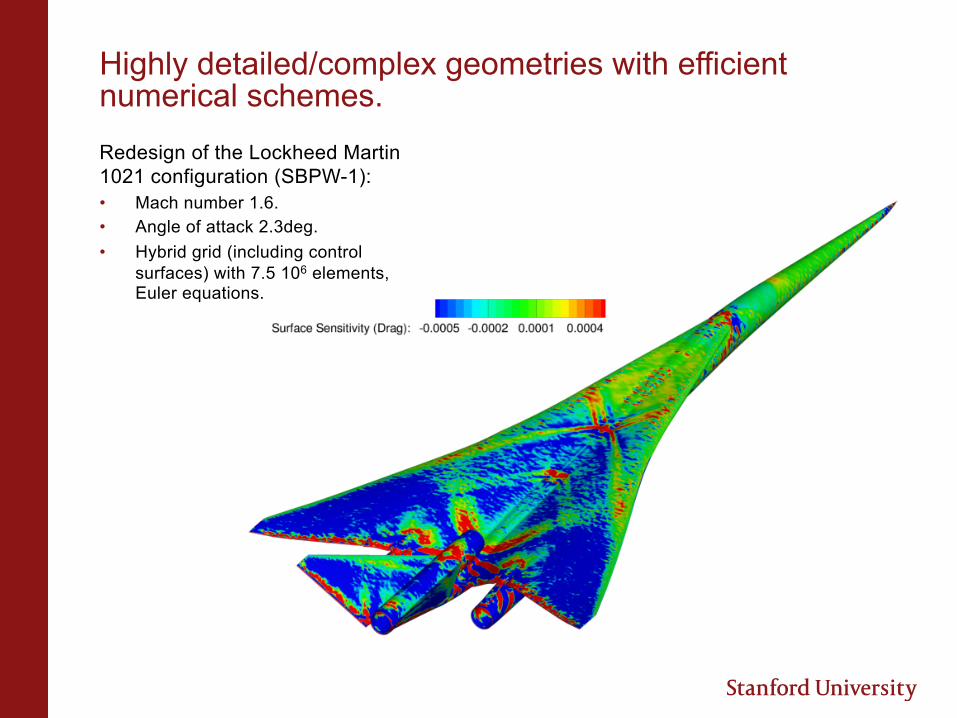
Highly detailed/complex geometries with efficient numerical schemes. Redesign of the Lockheed Martin 1021 configuration (SBPW-1): •  Mach number 1.6. •  Angle of attack 2.3deg. •  Hybrid grid (including control

surfaces) with 7.5 106 elements, Euler equations.

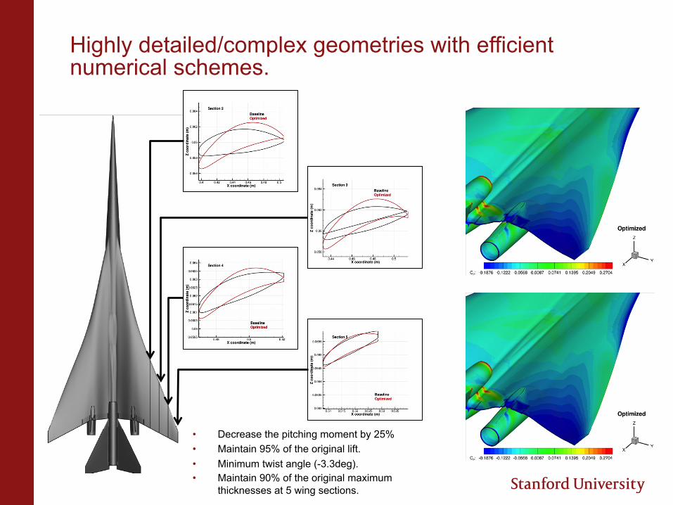
Highly detailed/complex geometries with efficient numerical schemes.

•  Decrease the pitching moment by 25% •  Maintain 95% of the original lift. •  Minimum twist angle (-3.3deg). •  Maintain 90% of the original maximum

thicknesses at 5 wing sections.

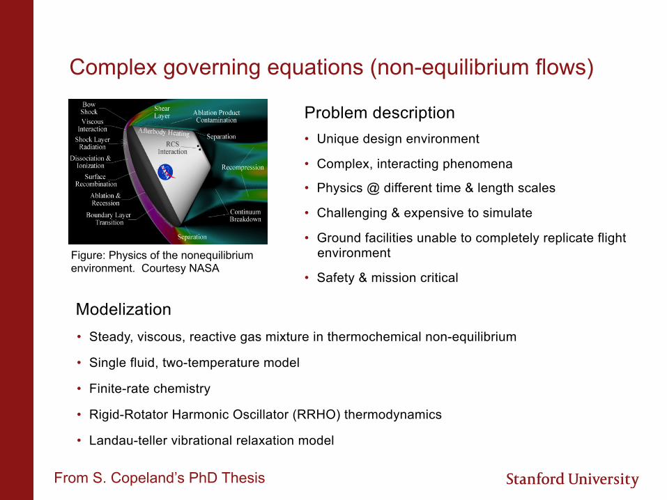
Problem description •  Unique design environment

•  Complex, interacting phenomena

•  Physics @ different time & length scales

•  Challenging & expensive to simulate

•  Ground facilities unable to completely replicate flight environment

•  Safety & mission critical

Complex governing equations (non-equilibrium flows)

Figure: Physics of the nonequilibrium environment. Courtesy NASA

Modelization

•  Steady, viscous, reactive gas mixture in thermochemical non-equilibrium

•  Single fluid, two-temperature model

•  Finite-rate chemistry

•  Rigid-Rotator Harmonic Oscillator (RRHO) thermodynamics

•  Landau-teller vibrational relaxation model

From S. Copeland’s PhD Thesis

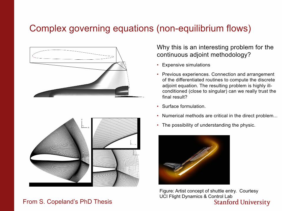
Complex governing equations (non-equilibrium flows)

Why this is an interesting problem for the continuous adjoint methodology? •  Expensive simulations

•  Previous experiences. Connection and arrangement of the differentiated routines to compute the discrete adjoint equation. The resulting problem is highly ill-conditioned (close to singular) can we really trust the final result?

•  Surface formulation.

•  Numerical methods are critical in the direct problem...

•  The possibility of understanding the physic.

Figure: Artist concept of shuttle entry. Courtesy UCI Flight Dynamics & Control Lab

From S. Copeland’s PhD Thesis

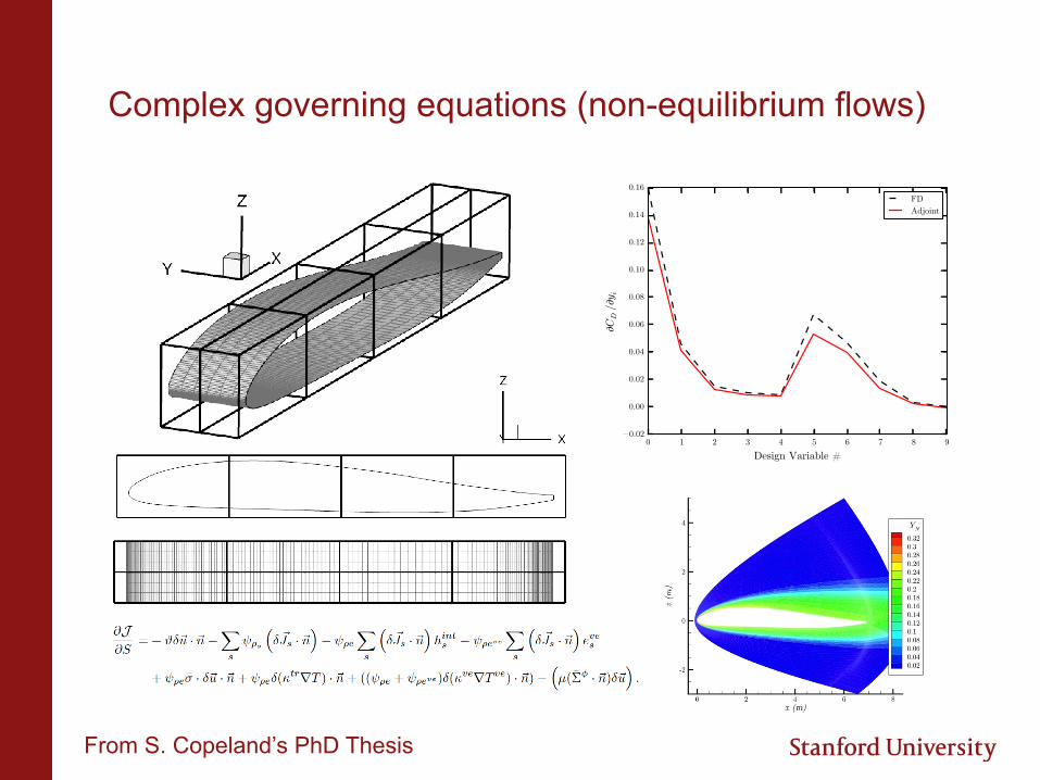
Complex governing equations (non-equilibrium flows)

From S. Copeland’s PhD Thesis

I N T R O D U C T I O N

S U R FA C E F O R M U L AT I O N

C O M P L E X S Y S T E M S

U N S T E A D Y D E S I G N

D E S I G N W I T H D I S C O N T I N U I T I E S

C O N C L U S I O N S

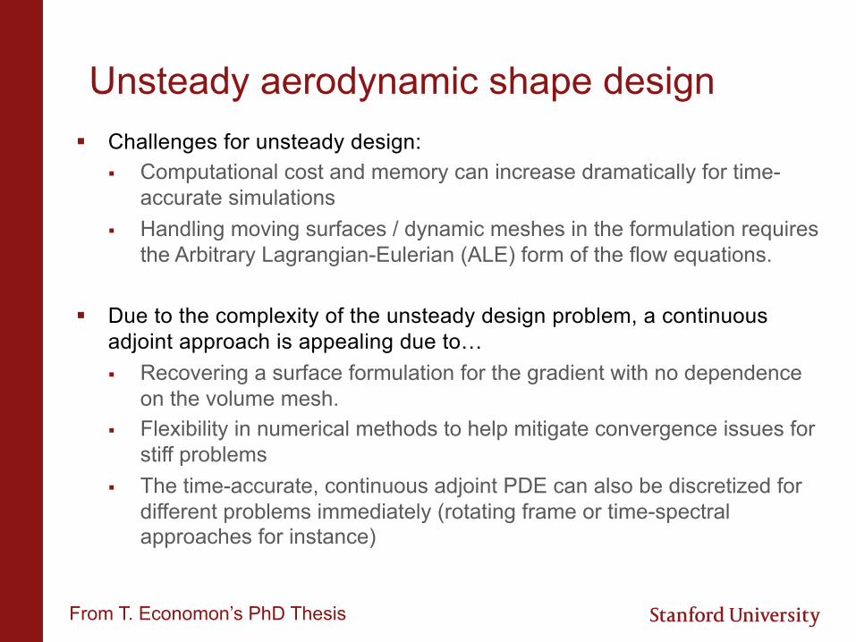
§  Challenges for unsteady design: §  Computational cost and memory can increase dramatically for time-

accurate simulations §  Handling moving surfaces / dynamic meshes in the formulation requires

the Arbitrary Lagrangian-Eulerian (ALE) form of the flow equations. §  Due to the complexity of the unsteady design problem, a continuous

adjoint approach is appealing due to… §  Recovering a surface formulation for the gradient with no dependence

on the volume mesh. §  Flexibility in numerical methods to help mitigate convergence issues for

stiff problems §  The time-accurate, continuous adjoint PDE can also be discretized for

different problems immediately (rotating frame or time-spectral approaches for instance)

Design in Unsteady Flows Unsteady aerodynamic shape design

From T. Economon’s PhD Thesis

Pitching Wing

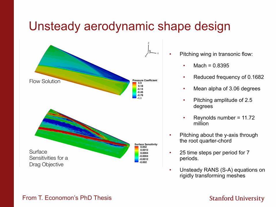
Flow Solution

Surface Sensitivities for a Drag Objective

Unsteady aerodynamic shape design

From T. Economon’s PhD Thesis

•  Pitching wing in transonic flow:

•  Mach = 0.8395

•  Reduced frequency of 0.1682

•  Mean alpha of 3.06 degrees

•  Pitching amplitude of 2.5 degrees

•  Reynolds number = 11.72 million

•  Pitching about the y-axis through the root quarter-chord

•  25 time steps per period for 7 periods.

•  Unsteady RANS (S-A) equations on rigidly transforming meshes

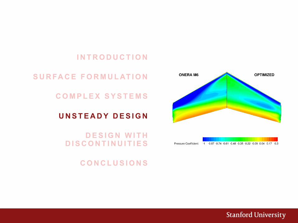
Pitching Wing Unsteady aerodynamic shape design ONERA M6

20.3 % Reduction in Time-averaged Drag

25 upper surface control point variables

RANS (S-A) (incidence of max drag)

From T. Economon’s PhD Thesis

I N T R O D U C T I O N

S U R FA C E F O R M U L AT I O N

C O M P L E X S Y S T E M S

U N S T E A D Y D E S I G N

D E S I G N W I T H D I S C O N T I N U I T I E S

C O N C L U S I O N S

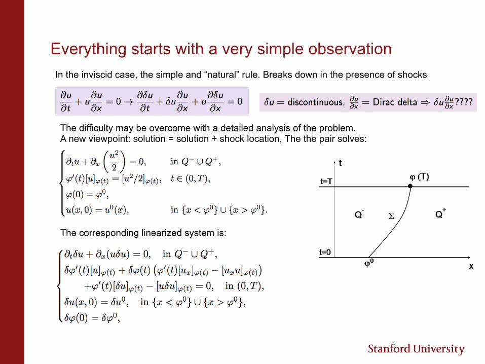
Everything starts with a very simple observation In the inviscid case, the simple and “natural” rule. Breaks down in the presence of shocks

The difficulty may be overcome with a detailed analysis of the problem. A new viewpoint: solution = solution + shock location, The the pair solves:

The corresponding linearized system is:

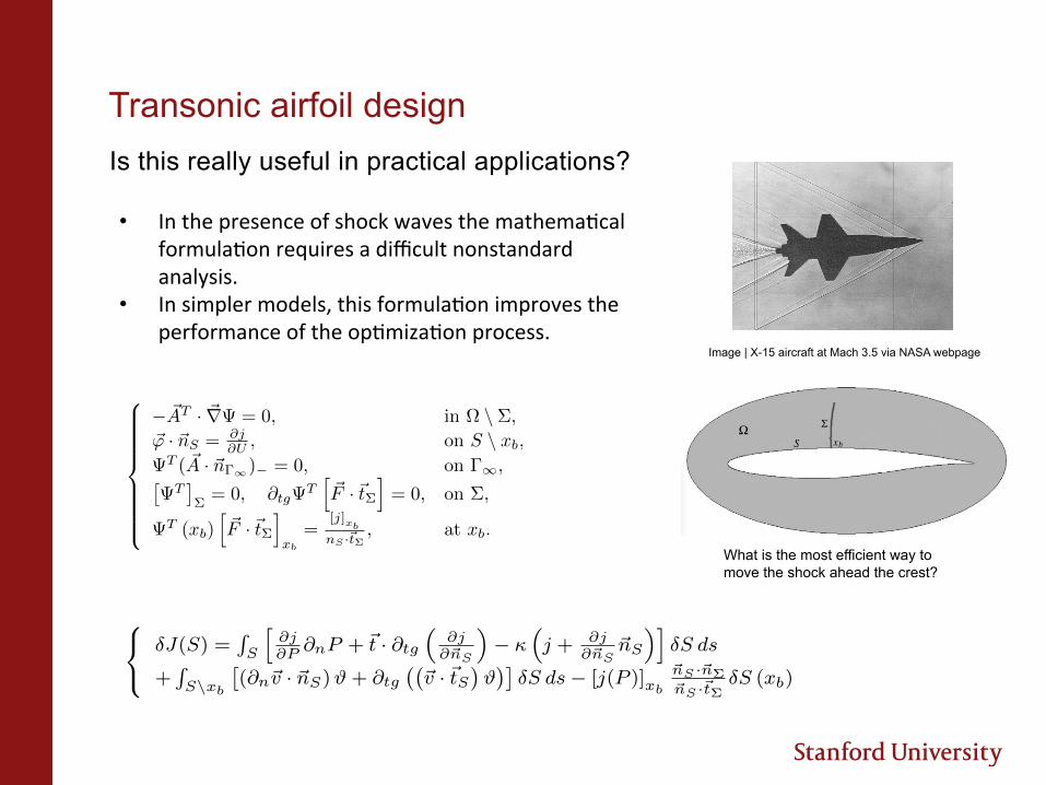
Transonic airfoil design Is this really useful in practical applications? •  In  the  presence  of  shock  waves  the  mathema2cal  

formula2on  requires  a  difficult  nonstandard  analysis.  

•  In  simpler  models,  this  formula2on  improves  the  performance  of  the  op2miza2on  process.  

Image | X-15 aircraft at Mach 3.5 via NASA webpage

8>>>>>>><

>>>>>>>:

� ~

A

T · ~r = 0, in ⌦ \ ⌃,~' · ~n

S

=

@j

@U

, on S \ xb

,

T

(

~

A · ~n�1)� = 0, on �1,

⇥

T

⇤⌃= 0, @

tg

T

h~

F · ~t⌃i= 0, on ⌃,

T

(x

b

)

h~

F · ~t⌃i

x

b

=

[j]x

b

n

S

·~t⌃, at x

b

.

• Euler equations:

8<

:

@

x

F

x

(U) + @

y

F

y

(U) = 0, in ⌦

~v · ~nS

= 0, in S

(F

x

, F

y

) · ~n⌃ = 0, on ⌃

U = (⇢, ⇢u, ⇢v, ⇢E)

T

• Cost functional: J(S) =

RS

j(p,~n

S

)ds,

• Adjoint system:

8>>>><

>>>>:

~r ·⇣~

A �U

⌘= 0, in ⌦ \ ⌃,

�~v · ~nS

= ��S @

n

~v · ~nS

+ (@

tg

�S)~v · ~tS

, on S \ x

b

, ,

(�W )+ = 0, on �1,h~

A(�⌃ @

n

U + �U)

i

⌃· ~n⌃ +

h~

F

i

⌃· �~n⌃ = 0 on ⌃,

• Derivative of the cost functional:

8<

:�J(S) =

RS

h@j

@P

@

n

P +

~

t · @tg

⇣@j

@~nS

⌘�

⇣j +

@j

@~nS~n

S

⌘i�S ds

+

RS\xb

⇥(@

n

~v · ~nS

)#+ @

tg

��~v · ~t

S

�#

�⇤�S ds� [j(P )]

xb

~nS ·~n⌃~nS ·~t⌃

�S (x

b

)

What is the most efficient way to move the shock ahead the crest?

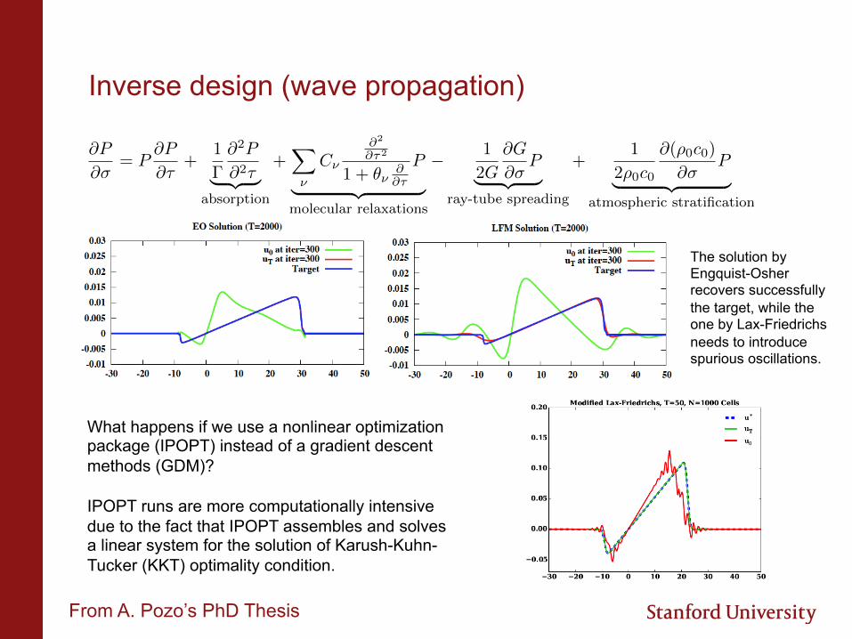
Inverse design (wave propagation)

The solution by Engquist-Osher recovers successfully the target, while the one by Lax-Friedrichs needs to introduce spurious oscillations.

What happens if we use a nonlinear optimization package (IPOPT) instead of a gradient descent methods (GDM)? IPOPT runs are more computationally intensive due to the fact that IPOPT assembles and solves a linear system for the solution of Karush-Kuhn-Tucker (KKT) optimality condition.

From A. Pozo’s PhD Thesis

@P

@�= P

@P

@⌧+

1

�

@2P

@2⌧| {z }absorption

+X

⌫

C⌫

@2

@⌧2

1 + ✓⌫@@⌧

P

| {z }molecular relaxations

� 1

2G

@G

@�P

| {z }ray-tube spreading

+1

2⇢0c0

@(⇢0c0)

@�P

| {z }atmospheric stratification

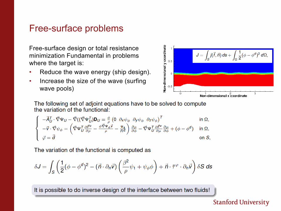
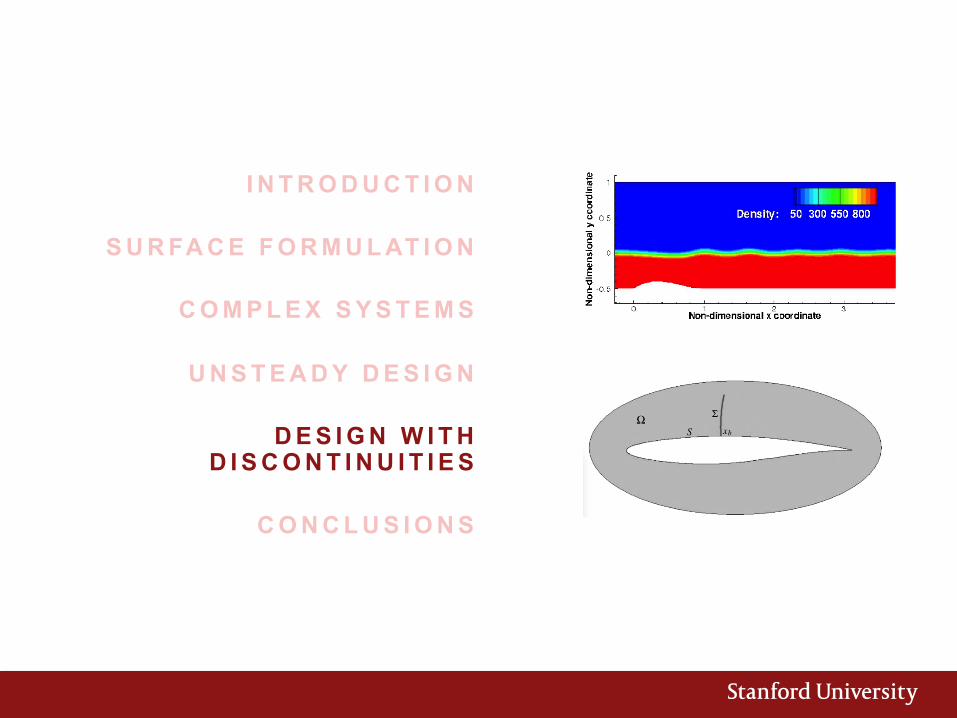
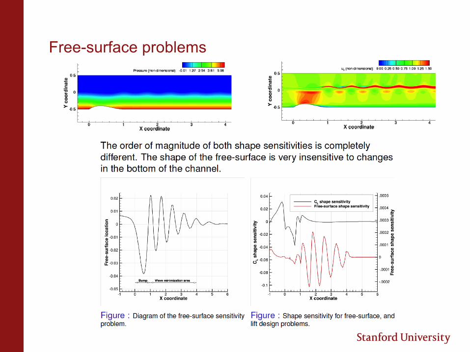
Free-surface problems

Free-surface design or total resistance minimization Fundamental in problems where the target is: •  Reduce the wave energy (ship design). •  Increase the size of the wave (surfing

wave pools)

Free-surface problems

I N T R O D U C T I O N

S U R FA C E F O R M U L AT I O N

C O M P L E X S Y S T E M S

U N S T E A D Y D E S I G N

D E S I G N W I T H D I S C O N T I N U I T I E S

C O N C L U S I O N S

Conclusions

Aerodynamic Optimal Shape Design, created and developed by Prof. Jameson, is a high-impact field with a need for sophisticated engineering, mathematical and computational developments. •  Prof. Jameson legacy is an example about how the intelligence, enthusiasm and

perseverance make miracles. With very limited computational resources he did some simulations that even today are difficult to repeat. Demonstrating that, from the point of view of success, what is expensive, requires time, patience and spirit are not the instruments but the ability to develop and mature an exemplary aptitude.

•  In the internet era it is “easy” to find people with an empty knowledge: they know a lot of information that you can easily find in 5 second using your smartphone. But, Prof. Jameson knowledge is completely different and impossible to find in other places.

•  The intelligence loves to learn, discover, and create new things. But, to achieve its owns objectives the personal intelligence should collaborate with the objectives of other people. The result of this collaboration is a real school of CFD, all inspired by Prof. Jameson generosity and talent.

The continuous adjoint strikes back

Francisco Palacios

(with results from S. Copeland, T. Economon and A. Pozo PhD thesis)

Department of Aeronautics & Astronautics Stanford University

A J 8 0 T H

S TA N F O R D U N I V E R S I T Y N O V E M B E R 2 1 S T , 2 0 1 4