The Consumer Price Index and the Measurement of … · ALAN S. BLINDER Princeton University and National Bureau of Economic Research The Consumer Price Index and the Measurement of

ALAN S. BLINDER

Princeton University and National Bureau of Economic Research

The Consumer Price Index and the Measurement of Recent Inflation

THE consumer price index in the United States may be the most closely watched economic barometer in the world. Yet in recent years, as the public and the media have paid increasing attention to the monthly CPI announcements, more and more economists and officials have ex- pressed dissatisfaction with the way the CPI measures inflation. The construction of price indexes, once an arcane subject used to torture graduate students, is now a subject debated in the halls of Congress and discussed on the nightly television news. In the wake of the stunning recent gyrations in the CPI inflation rate, this seems an opportune time to reexamine the index-and especially its treatment of housing, which has been so much in the public eye of late.

The first three rows of table 1 give a hint both that something is amiss, and that the problem is of recent vintage. The all-items CPI and the implicit deflator for personal consumption expenditures (hereafter PCE deflator) differ in numerous ways. The PCE deflator counts only currently produced consumer goods and services, and-at least in principle-includes them all; the CPI is based on a selected list of about 250 items, including several important used items (used cars, resold houses). The PCE deflator uses current-period weights (a Paasche index), while the

I thank Henry J. Aaron, Stephen M. Goldfeld, Daniel Hamermesh, Walter F. Lane, Frank de Leeuw, Jack E. Triplett, and members of the Brookings panel for helpful conversations and Danny Quah for research assistance. Research support from the National Science Foundation is gratefully acknowledged.

0007-2303/80/0002-0539$01.00/0 t? Brookinigs Institution

540 Brookings Papers on Economic Activity, 2:1980

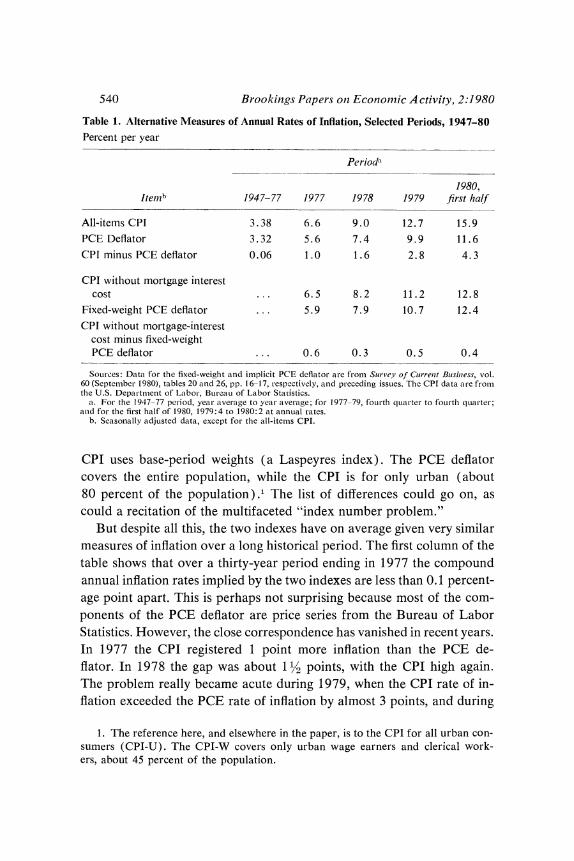
Table 1. Alternative Measures of Annual Rates of Inflation, Selected Periods, 1947-80 Percent per year

Perioda

1980, ltem?lb 1947-77 1977 1978 1979 first half

All-items CPI 3.38 6.6 9.0 12.7 15.9 PCE Deflator 3.32 5.6 7.4 9.9 11.6

CPI minus PCE deflator 0.06 1.0 1.6 2.8 4.3

CPI without mortgage interest cost ... 6.5 8.2 11.2 12.8

Fixed-weight PCE deflator ... 5.9 7.9 10.7 12.4

CPI without mortgage-interest cost minus fixed-weight PCE deflator ... 0.6 0.3 0.5 0.4

Sources: Data for the fixed-weight and implicit PCE deflator are from Surve,y of Cuirrentt Businiess, vol. 60 (September 1980), tables 20 anid 26, pp. 16-17, respectively, and preceding issues. The CPI data are from the U.S. Department of Labor, Bureau of Labor Statistics.

a. For the 1947-77 pet-iod, year average to year average; for 1977-79, fourth quarter to fourth qualter; anld for the first half of 1980, 1979:4 to 1980:2 at annual rates.

b. Seasonally adjusted data, except for the all-items CPI.

CPI uses base-period weights (a Laspeyres index). The PCE deflator covers the entire population, while the CPI is for only urban (about 80 percent of the population).' The list of differences could go on, as could a recitation of the multifaceted "index number problem."

But despite all this, the two indexes have on average given very similar measures of inflation over a long historical period. The first column of the table shows that over a thirty-year period ending in 1977 the compound annual inflation rates implied by the two indexes are less than 0.1 percentage point apart. This is perhaps not surprising because most of the components of the PCE deflator are price series from the Bureau of Labor Statistics. However, the close correspondence has vanished in recent years. In 1977 the CPI registered 1 point more inflation than the PCE deflator. In 1978 the gap was about 11/2 points, with the CPI high again. The problem really became acute during 1979, when the CPI rate of inflation exceeded the PCE rate of inflation by almost 3 points, and during

1. The reference here, and elsewhere in the paper, is to the CPI for all urban consumers (CPI-U). The CPI-W covers only urban wage earners and clerical workers, about 45 percent of the population.

Alan S. Blinder 541

the first half of 1980, when the gap was about 4 points. These numbers suggest that there may be problems with the CPI.

This paper focuses on two of these problems: the CPI's use of fixed weights in a period when large relative price changes are leading to substantial adjustments in spending patterns and its treatment of homeownership (and especially mortgage interest) costs. The last three rows of table 1 show that these two features of the CPI explain many of the discrepancies between the two indexes. The fourth row adjusts the CPI by removing mortgage interest costs; because 1977-80 was a period of rising interest rates, this adjustment results in less inflation each year. The fifth row reports the rates of change of the Bureau of Economic Analysis's fixed- weight version of the PCE deflator; as index number theory leads one to expect, the growth rate of this fixed-weight deflator always exceeds that of the standard PCE deflator (see below). By comparison with the numbers in the first three rows, the differences between the two indexes pre- sented in the last three rows are quite small indeed-almost always less than half a percentage point.

The Weighting Issue

Any overall price index is a weighted average of its constituent parts. There are three basic decisions to be made: what items to include, how much weight to assign to each item; and whether to use fixed (base-period) weights or variable (current-period) weights. The first two decisions con- stitute the choice of the so-called market basket; the third is the choice between a Laspeyres and a Paasche index.

Except for the issue of how much weight to place on homeownership, which I take up in the following section, I have little to say about the market basket. Although it would be conceptually superior to include all consumer goods and services (instead of 80 percent), the CPI's market basket is probably broad enough and sufficiently well selected (based on two comprehensive expenditure surveys in 1972-74) to measure very ac- curately the increase in income necessary to buy any reasonably representative market basket.2

2. U.S. Department of Labor, Bureau of Labor Statistics, Consumer Expendi- ture Survey: Interviewsn Sutrvey, 1972-73, Bulletin 1997 (U.S. Government Printing Office, 1978) and Consumer Expenditure Survey: Diary Survey, July 1972-June 1974, Bulletin 1959 (GPO, 1977).


The real issue is whether to use a fixed market basket or an evolving one. As everyone who has ever been a graduate student of economics knows, a Laspeyres index (such as the CPI) tends to overstate inflation relative to a "true" cost-of-living index while a Paasche index (such as the PCE deflator) tends to understate it. The reason is simple to explain. When different prices rise at different rates, consumers have the opportunity to escape part of the burden of inflation by buying substitutes for the goods whose prices are escalating most rapidly. The Laspeyres index ignores this possibility and therefore exaggerates the utility loss from inflation. The Paasche index assumes, equally incorrectly, that these substitutions entail no loss of satisfaction, and hence understates the burden of inflation.

Since the CPI is a Laspeyres index and the PCE deflator is a Paasche index, we should not be surprised if the former shows higher inflation than the latter. (The comparison is not a clean one, however, because the two market baskets differ.) This has been known for years-and has been thought unimportant. There was probably good reason to think so because the first column of table I shows that the CPI rose only trivially faster than the PCE deflator from 1947 to 1977.

A cleaner comparison between Paasche and Laspeyres indexes is ob- tained by looking at the PCE deflator and a fixed-weight PCE deflator. The compound annual rate of increase of the latter between 1958 (when it began) and 1977 was 3.71 percent while that of the former was 3.80 percent. It is hard to take this difference seriously. But recent performance appears to have departed from this pattern. The rate of increase of the fixed-weight PCE deflator exceeded that of the conventional PCE deflator by 0.3, 0.5, 0.8, and 0.8 percentage point in 1977, 1978, 1979, and the first half of 1980, respectively (see table 1).

These differences, however, reflect more than the pure difference between a Laspeyres and a Paasche index. To understand why, it is necessary to introduce some of the arithmetic of price indexes. Begin with the simplest case, that of a fixed-weight index such as the CPI or the fixed- weight PCE deflator. Such an index is a weighted average of its components. With Pt denoting the overall index and Pit the components, the expression is

(1) Pt = E~ WPiopit5

where the wi, are the base-period expenditure weights:

(2) Wi0 = xioCio zo pioi

Alan S. Blinder 543

where cit is the quantity of the ith item consumed in the tth period. If the shorthand notation Pt and Pit indicate one-period proportional rates of change, some straightforward computations of (1) yield

(3) - - i

where rit is called the relative importance of item i in period t and is defined by

(4) 'it = Wio Pt-, Pt-i

The PCE deflator is a current-period-weight index defined by

(5) Pt = p Cit =- WitpiJu p2 iocit

where

(6) Wit 1 pioCit pio L,I piocit'

are the (variable) weights.3 A little algebra shows that the rate of change of the PCE deflator can be written

(7) Pt I Pi,t-1p2 t + X, Pi t-i Pit Vit5 t t ~~~pi,t-i

where

(8) Pit - EC = vit

,2 PitCit -Pt

are the period t expenditure weights and wit is defined as the percentage rate of change of wit. Comparing equation 7 with 3 reveals two major differences. First, equation 7 contains a second sum that does not appear in 3. This is called (for obvious reasons) the "contribution of shifting weights," and if it is removed from the index one obtains the rate of change of what is called the PCE chain index. The chain index is basically a one-period Laspeyres index, which takes as its relative importances for period t the expenditure weights of period t - 1 and updates these weights each period. That these relative importances differ from those used in 3 is the second source of difference between the PCE deflator and the CPI.4

3. By convention, all pi, are set to unity, so wit is the weight in real expenditure. 4. In the case of constant weights, the Pi,t-1 in equation 7 and the rit in 3 are

equal. (This follows from equations 8 and 4.)

544 Brookings Pavers on Economic Activity. 2:1980

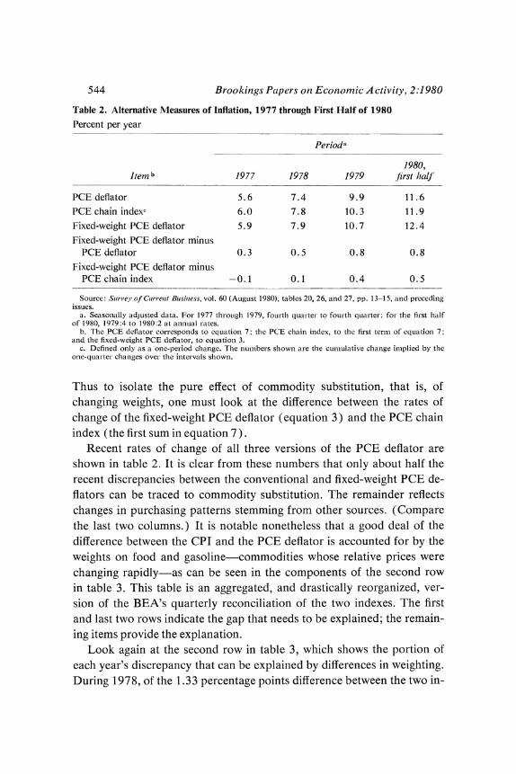
Table 2. Alternative Measures of Inflation, 1977 through First Half of 1980

Percent per year

Perioda

1980, Item b 1977 1978 1979 first half

PCE deflator 5.6 7.4 9.9 11.6

PCE chain indexc 6.0 7.8 10.3 11.9 Fixed-weight PCE deflator 5.9 7.9 10.7 12.4 Fixed-weight PCE deflator minus

PCE deflator 0.3 0.5 0.8 0.8 Fixed-weight PCE deflator minus

PCE chain index -0. 1 0.1 0.4 0.5

Source: Sur'efi' of Curr-l enit Bulsiniess, vol. 60 (AuguLst 1980), tables 20, 26, and 27, pp. 13-15, and preceding issues.

a. Seasonally adjusted data. For 1977 throuLgh 1979, fourth quarter to fourth quLarter; for the first half of 1980, 1979:4 to 1980:2 at annual rates.

b. The PCE deflator corresponds to equation- 7; the PCE chain index, to the first term-- of equation 7; and the fixed-weight PCE deflator, to equation 3.

c. Defined only as a one-period change. The numl-bers shown are the cumulative change im--plied by the one-quarter changes over the intervals shown.

Thus to isolate the pure effect of commodity substitution, that is, of changing weights, one must look at the difference between the rates of change of the fixed-weight PCE deflator (equation 3) and the PCE chain index (the first sum in equation 7).

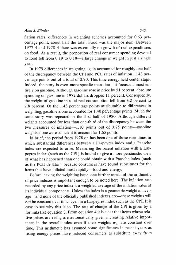
Recent rates of change of all three versions of the PCE deflator are shown in table 2. It is clear from these numbers that only about half the recent discrepancies between the conventional and fixed-weight PCE de- flators can be traced to commodity substitution. The remainder reflects changes in purchasing patterns stemming from other sources. (Compare the last two columns.) It is notable nonetheless that a good deal of the difference between the CPI and the PCE deflator is accounted for by the weights on food and gasoline-commodities whose relative prices were changing rapidly-as can be seen in the components of the second row in table 3. This table is an aggregated, and drastically reorganized, version of the BEA's quarterly reconciliation of the two indexes. The first and last two rows indicate the gap that needs to be explained; the remaining items provide the explanation.

Look again at the second row in table 3, which shows the portion of each year's discrepancy that can be explained by differences in weighting. During 1978, of the 1.33 percentage points difference between the two in-

Alan S. Blinder 545

flation rates, differences in weighting schemes accounted for 0.63 percentage point, about half the total. Food was the major item. Between 1977:4 and 1978:4 there was essentially no growth of real expenditures on food. As a result, the proportion of real consumer spending devoted to food fell from 0.19 to 0.1 8-a large change in weight in just a single year.

In 1979 differences in weighting again accounted for roughly one-half of the discrepancy between the CPI and PCE rates of inflation: 1.43 percentage points out of a total of 2.90. This time energy held center stage. Indeed, the story is even more specific than that-it focuses almost entirely on gasoline. Although gasoline rose in price by 51 percent, absolute spending on gasoline in 1972 dollars dropped 11 percent. Consequently, the weight of gasoline in total real consumption fell from 3.2 percent to 2.8 percent. Of the 1.43 percentage points attributable to differences in weighting, gasoline alone accounted for 1.40 percentage points. Much the same story was repeated in the first half of 1980. Although different weights accounted for less than one-third of the discrepancy between the two measures of inflation-1.10 points out of 3.75 points-gasoline weights alone were sufficient to account for 1.65 points.

In brief, the period from 1978 on has been one of those rare times in which substantial differences between a Laspeyres index and a Paasche index are expected to arise. Measuring the recent inflation with a Las- peyres index (such as the CPI) is bound to give a more pessimistic view of what has happened than one could obtain with a Paasche index (such as the PCE deflator) because consumers have found substitutes for the items that have inflated most rapidly-food and energy.

Before leaving the weighting issue, one further aspect of the arithmetic of price indexes is important enough to be noted here. The inflation rate recorded by any price index is a weighted average of the inflation rates of its individual components. Unless the index is a geometric weighted average-and none of the officially published indexes are-these weights will not be constant over time, even in a Laspeyres index such as the CPI. It is easy to see why this is so. The rate of change of the CPI is given by a formula like equation 3. From equation 4 it is clear that items whose relative prices are rising are automatically given increasing relative importance in the overall index even if their weights wit are constant over time. This arithmetic has assumed some significance in recent years as

rising energy prices have induced consumers to substitute away from

,-o Cu f'f -.-4l\ tn'~-0 o Nnomm outno- C

0 t ? ? I ? ? ? ?l N m ? ?l 0 n -) O QO r -o o C Z0

r4) W-) v--4 ON ~ ~ ~ ~ ~~;5)

xi CZo 0

=0~~~~~~~~~~~ X

044 44i-

n

oOG00 z 0 ?c? f

O N = Z.) .*

6 CZ 04 0 O O- 0

0.

00 o

C=: a.booooooooooooQQo -; 4 ).

C4 00QQ00 'f)ef)00 r- cn )C) en C

.= ~ ~ O-i04C cioe oo Q ~

u . 00 e e O \

; R > < % , b~~~~~~~~; ; C *

U S ) 4 C?, do=CQ_Co?4l '

-4 C ? 4

oI ) Q o .

00~~~~~~~~~~~~~~~~~~~~~~ ON Z.~) N00 0

Q ? CT~'L. 0 ; CXE :

044

0 -

0

CU ~~~~~ Q555Q Q555 5 Q -~~~~~~~~~~ 0 t t)- 0

0.

o N 0~~~~~~~~~~~~~ 00

C-)

CU~ ~ ~~~~~~~~~~~~~~~~~~c> CU -~~~~~~~~~~~~~~~o

o 0 ~~~~~~~~~~~~~~~~~~C 4J2 00 )~~~~~~~~~~~c :l 0 a,0>

b = 0~~~~~~~~. 00 01) 0~~~~~>0

C 0 0 CZ 4)U

.0~~~~~~~~~~~~~~~~~~~~~~ "CU 4U~~~~~~~~~~~~~~~~~~~ 44 C

CU 0 >~~~~UU I U- 4 0 0t- - 4440 6~~~~~~~~U)4 0 4

4) .000 ~~~~~~~~.0 ~0 0> 01)'~~-~~ CU4)-i CU 4.) 0 -~~I; v C

- 0 o 0 0 > 'd C 0 0- 044

O Q ~ ~ ~o *.-. 4) * 0

.0 ~0 S - o~~~~~~~~~~~~~~~~~~'

4)d 0 U ( o-H

Alan S. Blinder 547

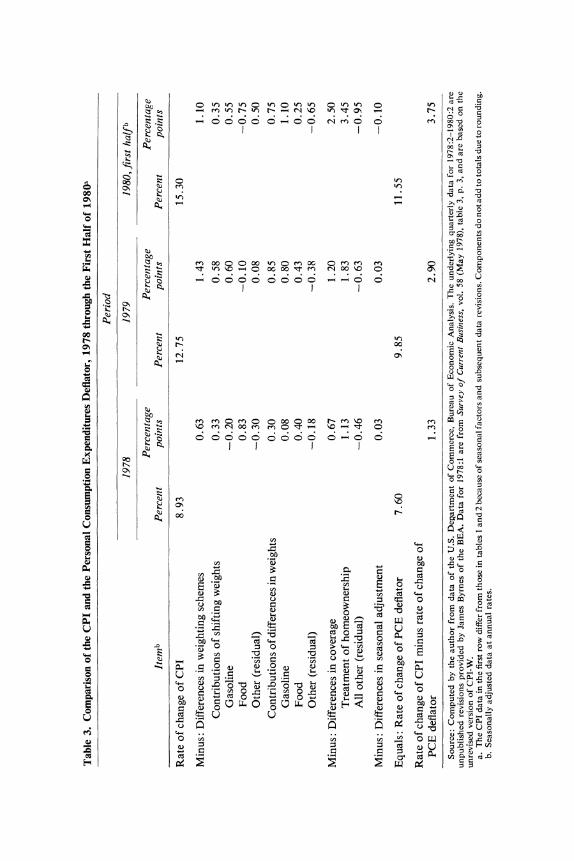
Table 4. Homeownership Costs and Overall Inflation, 1977 to First Half of 1980

Annual rate of inflation, in percent

Period

December December December December 1976- 1977- 1978- 1979-

December December December June Item 1977 1978 1979 1980a

Homeownership costs 9.2 12.4 19.8 24.7 All-items CPI 6.8 9.0 13.3 16.0

All-items CPI minus homeownership costs 6.1 8.0 11.3 13.2

Sources: Bureau of Labor Statistics, CPI Detailed Report, Junle 1980 (U.S. Government Printing Office, 1980), table 1, pp. 9-11, and similar preceding reports.

a. Not seasonally adjusted data at annuLal rates.

energy. For example, between 1976:4 and 1979:4 the share of energy in total nominal consumption rose only from 8.4 to 9.1 percent as consumers reacted to higher prices by buying less (the share in total real consumption fell from 6.7 to 5.8 percent). Despite this, the relative importance of energy in the CPI rose from 0.074 in December 1976 to 0.103 in De- cember 1979. Thus any given percentage increase in energy prices con- tributes about 40 percent more to the overall inflation rate today than it would have in 1977 even though consumers are spending only a slightly greater fraction of their current budgets on energy today. It is simply an arithmetic conclusion that the relative importances used to determine the average inflation rate must differ from the weights used to determine the average price level in the way prescribed by equation 4, which means that a fixed-weight index automatically assigns increasing relative importances to those items whose prices rise most rapidly.

The Homeownership Issue

The homeownership component of the CPI has contributed greatly to the recent gyrations in the CPI's inflation rate. (See table 4.) For example, it added 3 points to the inflation rate in the first half of 1980 and was chiefly responsible for the zero inflation rate recorded for July 1980.

The CPI and the PCE deflator treat homeownership costs very differently. Table 3 shows how much of the difference between the CPI and


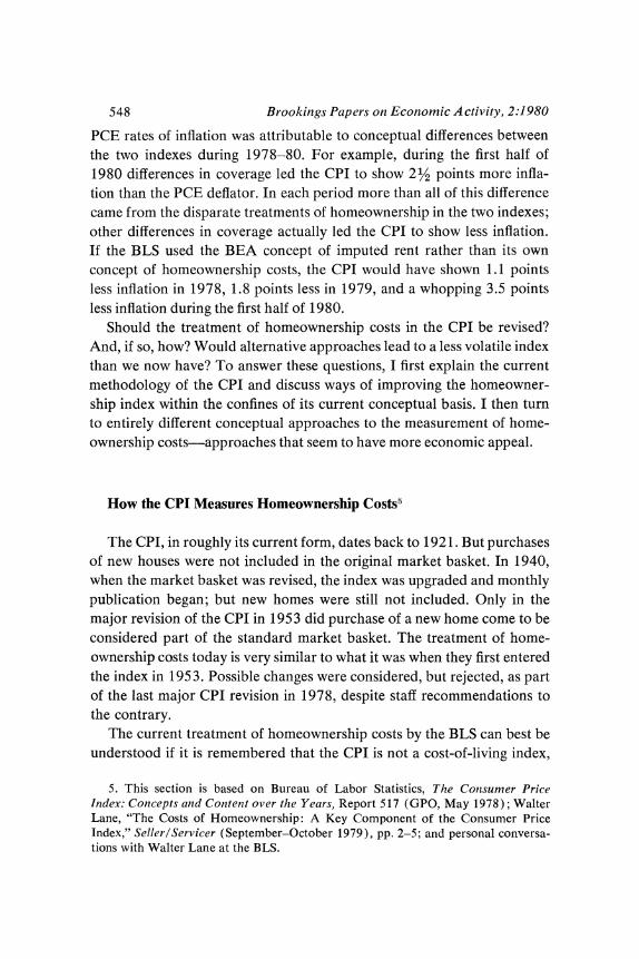
PCE rates of inflation was attributable to conceptual differences between the two indexes during 1978-80. For example, during the first half of 1980 differences in coverage led the CPI to show 21/2 points more inflation than the PCE deflator. In each period more than all of this difference came from the disparate treatments of homeownership in the two indexes; other differences in coverage actually led the CPI to show less inflation. If the BLS used the BEA concept of imputed rent rather than its own concept of homeownership costs, the CPI would have shown 1.1 points less inflation in 1978, 1.8 points less in 1979, and a whopping 3.5 points less inflation during the first half of 1980.

Should the treatment of homeownership costs in the CPI be revised? And, if so, how? Would alternative approaches lead to a less volatile index than we now have? To answer these questions, I first explain the current methodology of the CPI and discuss ways of improving the homeownership index within the confines of its current conceptual basis. I then turn to entirely different conceptual approaches to the measurement of homeownership costs-approaches that seem to have more economic appeal.

How the CPI Measures Homeownership Costs5

The CPI, in roughly its current form, dates back to 1921. But purchases of new houses were not included in the original market basket. In 1940, when the market basket was revised, the index was upgraded and monthly publication began; but new homes were still not included. Only in the major revision of the CPI in 1953 did purchase of a new home come to be considered part of the standard market basket. The treatment of homeownership costs today is very similar to what it was when they first entered the index in 1953. Possible changes were considered, but rejected, as part of the last major CPI revision in 1978, despite staff recommendations to the contrary.

The current treatment of homeownership costs by the BLS can best be understood if it is remembered that the CPI is not a cost-of-living index,

5. This section is based on Bureau of Labor Statistics, The Consunmer Price Index: Concepts and Content over the Years, Report 517 (GPO, May 1978); Walter Lane, "The Costs of Homeownership: A Key Component of the Consumer Price Index," Seller/Servicer (September-October 1979), pp. 2-5; and personal conversations with Walter Lane at the BLS.

Alan S. Blinder 549

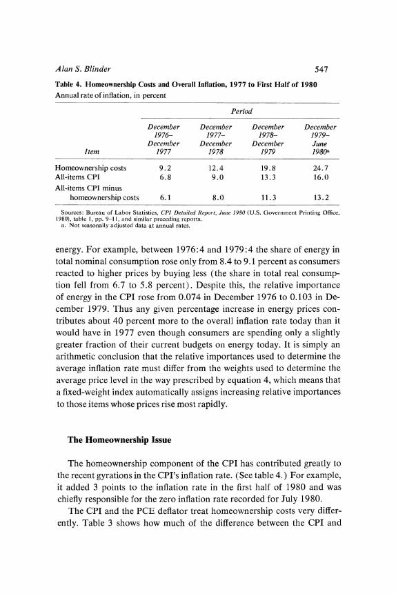
Table 5. Composition of the CPI Homeownership Index in December 1979 and Rate of Change of Its Components, December 1977 to June 1980

Relative Annual rate of Relative importance iii chanige, Decem-

importance in homeownership ber 1977 to all-items CPI, index componenzt, Junie 1980

Item December 1979 December 1979 (percent)a

Homeownership 0.249 1.000 17.7 Home purchase 0.104 0.417 13.0 Contractual mortgage interest cost 0.087 0.347 32.9 Property taxes 0.017 0.068 -0.4 Property insurance 0.006 0.022 11 . 1 Maintenance and repairs 0.036 0.145 10.9

Sources: BLS, CPI Detailed Report, June 1980 (GPO, 1980), tables I and 5, pp. 9-14, and similar preceding reports.

a. Not seasonally adjusted; calculations based on unrounded data.

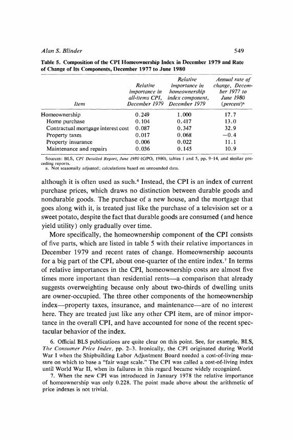
although it is often used as such.6 Instead, the CPI is an index of current purchase prices, which draws no distinction between durable goods and nondurable goods. The purchase of a new house, and the mortgage that goes along with it, is treated just like the purchase of a television set or a sweet potato, despite the fact that durable goods are consumed (and hence yield utility) only gradually over time.

More specifically, the homeownership component of the CPI consists of five parts, which are listed in table 5 with their relative importances in December 1979 and recent rates of change. Homeownership accounts for a big part of the CPI, about one-quarter of the entire index. In terms of relative importances in the CPI, homeownership costs are almost five times more important than residential rents-a comparison that already suggests overweighting because only about two-thirds of dwelling units are owner-occupied. The three other components of the homeownership index-property taxes, insurance, and maintenance-are of no interest here. They are treated just like any other CPI item, are of minor importance in the overall CPI, and have accounted for none of the recent spec- tacular behavior of the index.

6. Official BLS publications are quite clear on this point. See, for example, BLS, Thze Consuimer Price Index, pp. 2-3. Ironically, the CPI originated during World War I when the Shipbuilding Labor Adjustment Board needed a cost-of-living measure on which to base a "fair wage scale." The CPI was called a cost-of-living index until World War II, when its failures in this regard became widely recognized.

7. When the new CPI was introduced in January 1978 the relative importance of homeownership was only 0.228. The point made above about the arithmetic of price indexes is not trivial.


It is the two major components, home purchase and mortgage interest costs, that command our attention. Together they account for nearly 20 percent of the entire CPI, and they have contributed mightily to its recent volatility. How does the BLS divide monthly mortgage payments into two portions-one attributable to the price of a house and the other to the mortgage interest rate?

HOME PURCHASE

The cost of purchasing a new home enters the index just like the cost of any other good, with a weight determined by the 1972-73 expenditure survey and the 1972-74 diary survey. In computing the weight from the survey data, the BLS included the purchase price of homes bought in the survey year minus the selling price of homes sold in that year plus any transactions costs associated with these purchases and sales. In determining the weight of home purchase, resales of existing owner-occupied structures cancel, leaving only newly constructed homes or homes that, for some other reason such as conversions from rental status, enter the owner-occupied category for the first time.8

At first glance this seems a reasonable procedure. But on further re- flection the investment aspect of any durable good begins to muddy the waters. It seems clear enough that, if my neighbor and I had sold our homes to each other in 1973, the BLS should have ignored both transactions. However, consider the case of John Doe who bought his first house (a resale) in 1973 and lived in it until he died. Should a zero weight be given to Doe's purchase? It seems that it should not. After all, Doe did spend part of his budget on housing.

The reason for the difficulty is easy to pinpoint, but, I think, impossible to resolve within the BLS's conceptual framework. Houses are durable goods. In a very real sense, an individual "spends money" on housing as he lives in the house, not when he first buys it. If the BLS had adopted the economic approach and priced the service flow of this durable good instead of its purchase price, it would have ignored the house swap between my neighbor and me, and counted John Doe's flows of implicit expenditures on housing as he made them (that is, one year's worth would have been recorded in the survey year).

8. However, the prices of used homes certainly do count in the index (see below).

Alan S. Blinder 551

However, the BLS prices home purchases, not service flows. (I return to this below.) The weighting issue is probably unresolvable, given this conceptual treatment, because deciding whether to include or exclude resales is the same as deciding whether the seller of an existing house earns income from the sale or makes a negative expenditure. Standard CPI concepts call for ignoring the sale if it is construed as an income source, but including it if it is construed as a negative expenditure. I sub- mit that the distinction between earning positive income and making negative expenditures is extremely subtle.

Once a weight for home purchase is established, the next step is to derive a house price index to which this weight can be applied. The BLS now constructs its house price index from data on sales of houses with Federal Housing Administration financing. There are serious problems with these data. According to the BLS, "FHA-insured housing constitutes a small and unrepresentative segment of the market. In 1973, these FHA- guaranteed purchases represented only about 6 percent of the home purchase market."9 One reason for this is that the FHA mortgage ceiling, which is now $89,500, effectively eliminates all higher-priced housing from consideration. Another is that some areas (such as the Northeast) have very few FHA transactions. Each of these probably biases the rate of change of house prices, but possibly in opposite directions.10 The trunca- tion problem caused by the FHA mortgage ceiling is obvious. Even though the ceiling is periodically adjusted upward, preliminary work by the BLS suggests that this may have been a serious source of downward bias in recent years.11 On the other hand, underrepresentation of the Northeast probably biases the home price index upward. If it is true, as many ob- servers of the housing market suspect-that lower-priced homes have had faster rates of appreciation than higher-priced homes in recent years- then this, too, would impart an upward bias to the rate of change of the CPI home price index.12

On balance, while the potential biases are great, it is hard to guess how severe they may be or even in which direction they may go. In addition to the large potential bias, the small sample size in many cells makes sampling

9. BLS, The Conslunmer Price Inidex, p. 13. 10. In addition, processing delays mean that the CPI home-purchase index often

lags several months behind the actual data. 11. John S. Greenlees, "Hedonic Indexes of Home Purchase Prices: Preliminary

Report," Bureau of Labor Statistics (forthcoming). 12. This is stressed, for example, by Greenlees (ibid).


variance in the FHA data quite large and requires frequent imputations. A better source of data on house prices thus seems imperative. The BLS staff is, incidentally, well aware of the problems with the FHA data.

MORTGAGE COSTS

The other major component of the homeownership index-and by far the most troublesome one-is "contracted mortgage interest costs," a component that combines the home purchase prices just explained with an estimated mortgage interest rate.

To develop a representative mortgage interest rate, the BLS collects quotations from the Federal Home Loan Bank Board for mortgages closed during the first five business days of each month, and uses these quotations to construct a mortgage interest rate index for the following month.13 A one-month delay is built into this procedure: the July index records mortgages closed in June, and so on. There is no particular reason, other than historical inertia, for this data-processing lag.

But there is another, longer lag between changes in mortgage rates and their appearance in the CPI that is not so easily avoided. Mortgages closed in June probably correspond to mortgage commitments made mostly in March, April, and May. On average, the closings lag behind commitments by about two months; but the corresponding mortgage rates need not follow this lag mechanically. When rates are rising, April commitments closed in June will typically be at April interest rates. But when rates are falling it is more typical for banks to lower the rate to the current market rate; April commitments closed in June would carry the June interest rate. Thus the CPI mortgage interest rate index, which properly includes closing rates rather than commitments, may fall much more rapidly than it rises.14 The two lags in combination mean that changes in the CPI mortgage interest rate index lag behind changes in market interest rates by about three months on average.

13. The BLS does this for each of 240 cells: 40 geographical areas, 3 down payment classes, and a distinction between mortgages on new and existing homes. These conventional mortgages take 86.5 percent of the weight. The remaining 13.5 percent goes to the FHA and VA ceiling rates.

14. The July 1980 index provides an outstanding example. The mortgage interest rate index fell at an annual rate of 48 percent from June to July. This was enough to make the homeownership component of the CPI fall at an annual rate of 17 percent and cause the all-items index to be virtually unchanged despite rising prices of many other goods and services.

Alan S. Blinder 553

The procedure the BLS uses to attach a weight to their mortgage cost index seems quite odd. During the survey year, the BLS recorded the interest payments (not including amortization) that would be due over the first half of the lifetime of each new mortgage. These future contractual mortgage payments were simply added, with no discounting. Summing these payments across all units in the survey led to the weight for "contracted mortgage interest cost" in the CPI, which is thus highly dependent on the interest rates that prevailed during the base period.

An example will help clarify the procedure, and also explain why I view it as a serious case of double-counting (or possibly one-and-a-half counting). Consider a new home bought in 1972 for $40,000, a reasonably typical amount. If the down payment was $8,000 (20 percent), and a $32,000 mortgage was taken out at 71/2 percent interest, the annual mortgage payment (ignoring within-year compounding) would have been $2,834.72.15 Because the first half of the lifetime of the mortgage is 12.5 years, this means that the BLS would have included mortgage payments of 12.5 x 2834.72 = $35,434, minus $9,005 in amortization, or $26,429 in interest payments. Thus, when it came to determining the weight for homeownership, $40,000 would have been included in the "home purchase" component and another $26,429 in the "contracted mortgage interest cost" component. This strikes me as a serious case of overweighting, and we can be grateful that, for some reason, the BLS decided to include only half the mortgage payments, not all of them.16 When a family purchases a home it makes some down payment ($8,000 in the example) and commits itself to make future mortgage interest payments that are equal in discounted present value to the remainder of the purchase price ($32,000 in the example)-if the mortgage rate is used to do the discounting. Thus, it seems to me, if it is desired to split the total purchase into two components (home price and mortgage cost), a minimal require- ment should be that the two pieces together add up to the purchase price of the house ($40,000 in the example). The current treatment does not do anything like this, and as a result it would appear that the weight accorded to homeownership is seriously exaggerated in the index. This is particularly unfortunate because the homeownership component is so volatile. Furthermore, the treatment biases the whole CPI in periods in

15. The Federal Home Loan Bank Board's series on yields on new conventional mortgages was 7.6 percent in 1972. I use continuous compounding formulas here.

16. Between 1953 and 1964 all the mortgage payments were included.


which homeownership costs as measured in the index are rising at dra- matically different rates than other prices.

There is direct evidence that the relative importance of homeownership is exaggerated in the CPI. For example, in 1978 personal consumer expenditures on tenant-occupied nonfarm dwellings in the national income accounts amounted to $54.2 billion, while the corresponding figure for owner-occupied dwellings was $142.9 billion. The ratio of the latter to the former is 2.6. Yet the relative importances of owner-occupied and rental housing in the CPI during 1978 averaged 0.232 and 0.056, respectively. The corresponding ratio is 4.2, more than half again as large. Or consider the five experimental alternatives that the BLS has recently begun to publish as part of its monthly CPI release. In December 1977 the relative importance of the official homeownership index was 0.228, and it ranged from 0.087 to 0.145 for the five experimental alternatives.

Economic Approaches to Measuring Homeownership Costs

Everyone seems to agree that the current treatment of homeownership in the CPI is wrong. But there is less agreement on what should replace it.17 The goal, however, should be quite clear: an empirical counterpart is needed to the theoretical concept of the service flow of a durable good. This is quite different from the current CPI convention of including durable purchases when they are made.

RENTAL EQUIVALENCE

To an economist, the natural place to begin looking for an empirical measure of service flows is the rental market. Imputed rents on owner- occupied houses, for example, are included as a component of personal consumption expenditures in the national income accounts. The BLS has investigated this option in one of its experimental series-rental equivalence. This index is constructed by applying to the CPI rent index a weight derived from the estimated rental value of all owner-occupied homes in the 1972-73 Consumer Expenditure Survey. As anyone who has studied the CPI in recent years knows, the rent index is one of the CPI's slowest

17. I argue below that there is good reason for this disagreement.

Alan S. Blinder 555

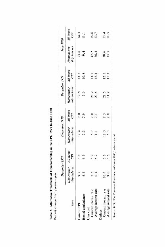
growing components.18 So it is not surprising that the rental equivalence approach yields a homeownership index that inflates much more slowly than the current official index (compare the homeownership indexes for the first two rows of table 6). Similarly, the overall CPI inflation rate for each year shown in the table would have been lower under the rental equivalence approach, and the 1977-80 acceleration of inflation would have been much less (compare the all-items CPI for the first two rows of the table).

But before I declare the BLS's problem solved, I should note that the CPI rent index is probably not appropriate for imputing rents to owner- occupied dwellings. The mix of housing types that are rented is very different in many respects (location, size, number of rooms, age, numbers of houses and apartments, and so on) from the mix of housing types that are owner-occupied. There is therefore no reason to believe that the levels of rents on rented dwellings are good proxies for imputed rent levels on owner-occupied dwellings. The story is less clear, however, for growth rates. The factor inputs used to build and maintain rented dwellings are, for the most part, the same as the factor inputs used to build and maintain owner-occupied dwellings. Thus if Tobin's "q" for rented houses and his "q" for owner-occupied houses were both constant at unity, there would be good reason to think that the growth rate of a properly weighted index of rents would approximate quite well the growth rate of imputed rents on owner-occupied dwellings. However, the two versions of q undoubtedly diverge from unity quite frequently, and need not move together in the short run. Thus rental equivalence is not without its perils.

In brief, although rental equivalence may be the conceptually correct approach, there are potentially serious problems in implementing it empirically by using directly observed rents. These are problems that the BLS should be and is working on. Specifically, answers are needed to the following questions. How good is the CPI rent index as an index of rental rates on rented dwellings? How well does an index of observed rental units serve as a proxy for the behavior of imputed rents on owner-occupied housing; that is, do the q on the two types of dwellings move more or less together? (It is easy to think of reasons why they might not-changes

18. In July 1980 the CPI rent index stood at 192.1 (1967 = 100), compared to the all-items CPI of 247.8. Some have argued that the CPI rent index understates the increase in rents because it fails to correct for the fact that its sample of dwellings grows older each year.

eX - Ul r- --4 14

00 (N- k

o: S U

~~~t en^

cn 00 a Cq -- C CN 00 tf 0 v

0 S aN or- 00 rno - eE'o ( X o N Ne

0~~~~~~~~~~~~~~~~~~0 00 ~ ~ ~ 00e l

- i 0 O~ 0~o XVn

o . C C t o

cJ R r.-- 0 e vo N

cZ s E _ oo en os r s m Z o

U. :0 (' U u 00

UN~ .

Alan S. Blinder 557

in tax laws are one example.) And how feasible is it for the BLS to find a sample of rented dwellings that matches the characteristics of the universe of owner-occupied dwellings?

I do not pretend to know the answers to these questions. If they turn out favorably, devising a new rent index more representative of owner- occupied dwellings has much to recommend it. If the BLS deems the task impossible, an economist naturally thinks next of user cost.

USER COST OF HOUSING

Measuring homeownership costs by a user-cost concept is another alternative that the BLS has considered. User cost was developed by Dale Jorgenson for a precisely analogous problem: industrial capital is normally purchased, not rented, and hence market rental rates were not available. Jorgenson's user cost of capital was meant to represent the rental rates that capital goods would command if they were rented. On the surface, it is not hard to modify Jorgenson's ideas for the case of housing. But, once again, there are difficulties in implementing it empirically.

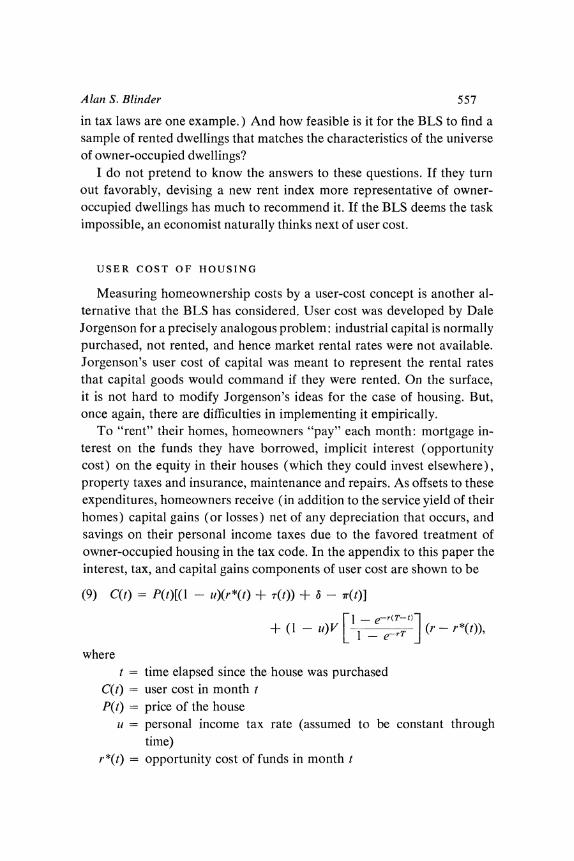
To "rent" their homes, homeowners "pay" each month: mortgage interest on the funds they have borrowed, implicit interest (opportunity cost) on the equity in their houses (which they could invest elsewhere), property taxes and insurance, maintenance and repairs. As offsets to these expenditures, homeowners receive (in addition to the service yield of their homes) capital gains (or losses) net of any depreciation that occurs, and savings on their personal income taxes due to the favored treatment of owner-occupied housing in the tax code. In the appendix to this paper the interest, tax, and capital gains components of user cost are shown to be

(9) C(t) = P(t)[(1 - u)(r*(t) + r(t)) + - r(t)]

1 - e-r(T-t) + (I1 - u) V _ e1-erT (' - " (t))

where t = time elapsed since the house was purchased

C(t) = user cost in month t P(t) = price of the house

ii = personal income tax rate (assumed to be constant through time)

r *(t) = opportunity cost of funds in month t


r = mortgage interest rate (assumed to be constant through time) T(t) = property tax rate (percent of true market value)

= depreciation rate (assumed to be constant through time) r(t) = accrued capital gains rate in month t

V = original face value of the mortgage T = duration of the mortgage.

Equation 9 differs from the standard user-cost formulation that is so familiar from the investment literature in two important respects. The first is that the equation includes actual ex post realized capital gains on the house rather than ex ante expected gains. This is appropriate because the objective is to develop a series representative of what it actually cost to own a particular house for the month under consideration, not to ascer- tain the relative price that should guide investment decisions. The second is the addition of the last term in 9, which merits discussion because it helps illuminate some of the issues.

Suppose initially that observed market rates on home mortgages are used as a proxy for the opportunity cost of funds.19 For new mortgages (t 0 O), the last term drops out because r* (0) = r. An issue arises, however, for old mortgages. Suppose also that interest rates have risen since the mortgage was taken out, so that r* (t) exceeds r and the last term in 9 is negative, implying that user cost is below what the standard formulation suggests. Why? The reason is that the standard user-cost formula charges homeowners the current market interest rate, r* (t), on both the funds they borrow from themselves (their equity in the houses) and the funds they borrow from the bank (their outstanding mortgage balances). But, in fact, while homeowners do implicitly pay r* (t) on their own equity, they do not pay r* (t) to the bank. The bank is locked into col- lecting r for the life of the mortgage. So when interest rates rise, homeowners receive part of the financing at a cheaper rate than they would in a world in which mortgage rates were renegotiable every period. Con- versely, if interest rates fall (r > r* (t) ), homeowners will pay more for credit than they would in a spot mortgage market unless they choose to

19. Robert Gillingham has argued persuasively that it would be better to use the internal rate of return on housing for r". However, to calculate this internal rate of return, it is necessary to know the equivalent rent. Hence Gillingham's point is actually an argument to use rental equivalence-if one can measure it. See Robert Gillingham, "Estimating the user cost of owner-occupied housing," Monthly Labor Review, vol. 103 (February 1980), pp. 31-35.

Alan S. Blinder 559

refinance and bring r down to r* (t). This is the meaning of the last term in 9.

Other practical issues arise in trying to make 9 operational. For example, what tax rates should be used and how would one measure depreciation? These are issues that the current BLS experimental user-cost series do not handle well. Improvement is needed; but I do not dwell on these issues here because there is a much broader issue to address. Would one expect a user-cost index, properly constructed along the lines of 9, to track the behavior of rental rates? The answer seems clearly to be no; and the reasons are quite instructive.

Because the current market interest rate and the one-period actual capital gains rate have such high weights in 9, the resulting user-cost series will be extremely volatile. (Some direct evidence on this is offered below.) Would market rental rates be this volatile if the houses now occupied by their owners were rented instead? I am quite confident that they would not be. Certainly the current market for rented dwellings ex- hibits no such volatility, and for good reasons. One is that the market for rental housing is not organized as a spot market, probably because the transactions costs of getting in and out are so immense. Even if there were no long-term contracts, it seems most unlikely that monthly rents would dance in tune with monthly fluctuations in interest rates or capital gains. The reason is that the market for rented housing is one in which the rental rate equilibrates the flow supply of housing services with the flow demand. Suppose the stock demand for housing rises. Will rents jump immediately to "clear the market?" It is not likely. Instead, the prices of houses will increase enough (with corresponding effects on the user cost) to equate the stock demand with the (temporarily fixed) stock supply. Tobin's q will therefore be pushed above unity, encouraging the construction of more houses. The disequilibrium will persist until enough new houses have been built to reduce q back to unity. Rents might rise slightly during the adjustment period (a housing shortage), but they would not be expected to rise much.

These "hunches" are backed by direct evidence that the user costs are too volatile to represent market rents. In his paper in this issue, Hender- shott calculates a user-cost series for rented dwellings that is conceptually similar to my equation 9. When this series is compared with the actual observed rental rates in that market (see his figure 1), it is clear that the former is far more volatile than the latter.


How much differently would the CPI have behaved in recent years if the BLS had adopted user cost in place of its current treatment of homeownership? The BLS currently has two experimental user-cost series; one uses current mortgage interest rates, the other, a fifteen-year weighted average of mortgage rates. However, the weighting scheme, which reflects the age distribution of existing mortgages, is heavily front-loaded: 31 percent of the weight is on the first 1 1/2 years and 69 percent is on the first 51/2 years. So the two series behave more similarly in practice than might be expected. The recent behavior of the two series is summarized under "user cost" in table 6.

In 1977 and 1978, substitution of user cost for current BLS methods would have led to a smaller measured inflation rate, as expected. Under present concepts, the rates of increase of homeownership costs in the two years were 9.2 and 12.4 percent, respectively. Under a user-cost measure, the corresponding rates would instead have been 2.5 and 5.7 percent using current mortgage rates or 0.4 and -1.1 percent using average mortgage rates. These are large differences. Using average mortgage rates would have reduced the overall inflation rates by about 1 percentage point in 1977 and 2 points in 1978, making them even slightly lower than under rental equivalence.

The tables turn in 1979 and 1980, however. The user-cost measures actually increased at a more rapid rate than the official homeownership index, and much faster than the rental equivalence measure. As expected, the user-cost measures seem to be inherently volatile. The volatility problem becomes particularly acute in periods, like the current one, in which the level of the user-cost series is quite low so that relatively small absolute changes in user cost correspond to very large relative changes. This follows from 9. For simplicity, suppose that u, T, and 8 are all constant, and that all mortgages bear the current interest rate, r(t) in each period. Then the user-cost formula becomes

C(t) = P(t)[(l - u)(r(t) + r) + r- (t)].

A straightforward calculation shows that the percentage change in user cost from one period to the next is given by

AC(t) AP(t) + (1 - u)r(t)P(t) Ar(t) _ [r(t)P(t)1 Ar(t) C(t) P(t) L C(t) r(t) L C(t) ] -(t)

As C(t) becomes very small, the weights attached to the changes in in-

Alan S. Blinder 561

terest and capital gains rates become quite large. (I wonder what the BLS does when C(t) becomes negative!)

This is not a nitpicking issue. In recent years, user-cost measures for owner-occupied housing have in fact been very low.20 It might be thought that this problem is finessed because items with low price tags are automatically given small expenditure weights in a price index. But as men- tioned above, the CPI is a Laspeyres index with 1972-74 as the base period. Thus the weight attached to C(t) depends on its average level in 1972-74 rather than on its (very low) current level.

This is where I came in. The perceived problem with the current CPI treatment of homeownership is that it is too volatile. Yet a user-cost series is likely to be even more volatile.21 The basic problem is inherent in using an interest rate as a component of a price index, and it turns out that user- cost measures assign even more importance to interest rates than does the current CPI methodology.

Conclusions: Improving the Measurement of Homeownership Costs

Nearly everyone seems to agree that the CPI provides a seriously dis- torted picture of changes in homeownership costs. Can it really make sense to state, as the index does, that the cost of homeownership rose at a 25 percent annual rate between December 1979 and June 1980 and then fell at an annual rate of 17 percent between June 1980 and July 1980? Can the picture be brought into sharper focus and the CPI tamed?

There are three basic candidates and none of them is especially ap- pealing. First, marginal improvements could be made in BLS procedures without in any way overhauling the basic conceptual framework that is currently in use. Among these would be to eliminate unnecessary lags in processing the mortgage rate data of the Federal Home Loan Bank Board and the FHA house price data; to use data on home prices from a broader, more representative sample than the FHA data; to replace the current

20. See, for example, the paper by Patric Hendershott in this issue. 21. The extreme volatility of the user-cost series is mitigated in part by the lower

weight (only about 0.10 to 0.11) accorded homeownership when the experimental user-cost formulations are employed. In 1979, for example, overall CPI inflation would have been about the same as in the official index if user cost with current mortgage rates had been used, and 1.2 points lower under user cost with average mortgage rates (see table 6).


mortgage interest rate with a long-term weighted average; and to reduce the weight on homeownership, which seems excessive on several grounds. These changes would not move the CPI's treatment of homeownership costs any closer to the treatment suggested by economic analysis, but they would at least reduce what now appears to be excessive volatility in homeownership costs. This is a prescription for powdering a nose when plastic surgery is probably needed.

Second, an effort could be made to develop a sample of rented dwellings that matches as closely as possible the universe of owner-occupied dwellings. As noted above, the job probably cannot be done perfectly. But the remaining shortcomings in the sample might be overcome by appropriate reweighting. It is quite possible that this technique, while far from the perfect solution, will be as close to a "true" measure of rental equivalence as we are likely to achieve, and this approach needs to be explored.

A third candidate is user cost. If measured correctly, user cost can indeed tell us how much it cost typical homeowners to use their homes in a given month. But that hardly makes it the ideal solution. I have argued at some length that a user-cost series is bound to be far more volatile than the rents that would emerge if the owner-occupied housing market were somehow transformed into a rental market.

But what does this mean? Market rents probably would be much less volatile than user cost. Yet user cost is the truer measure of the literal cost of living in one's house if it is owned rather than rented. The problem is that homeowners have a split personality-they are both consumers of housing services and investors in houses as assets. The two roles are inextricably bound together for owner-occupied houses, virtually by defi- nition. So it is not surprising that people have difficulty deciding which measure of homeownership costs is "correct."

Consider the example in which Dr. Jekyll rents a house from Mr. Hyde. The cost of owning the house for a month is C(t); implicitly, this is what Mr. Hyde pays. But it is not what he charges Dr. Jekyll. Dr. Jekyll's rent stream, call it R (t), will over a long period of time be equal in present value to Mr. Hyde's user-cost stream. But R (t) will reflect few if any of the monthly "blips" in C(t). Mr. Hyde, the entrepreneur, bears all the risk while Dr. Jekyll pays a steady monthly rent. There seem, then, to be two choices with claims to being correct. On the one hand, perhaps Mr. Hyde should be ignored; he is, in any case, an investor rather than a consumer. Then R(t), rental equivalence, should enter Dr. Jekyll's cost-of-

Alan S. Blinder 563

living index. On the other hand, Jekyll and Hyde do inhabit the same body (if at different times!) and thus perhaps they should be amalgamated and a cost of living should be computed for the pair. In this case one is led to user cost, C(t).

It is now the time to choose. I think the current treatment can be elimi- nated from serious contention. One need only think about the purposes for which the CPI is used to conclude that what is needed is a cost-of- living index based on a service-flow concept of housing, not a current ac- quisition price index that treats durable purchases as instantaneous consumption. Apart from the use of the CPI by economists (a small and unrepresentative group), it is used mostly for indexing various types of contracts to the price level-wages, social security benefits, and so on. For this purpose, it is clear that what is needed is a cost-of-living index rele- vant to the group involved (workers, old people, and so forth) rather than an abstract "current price" index. Similarly, economists and others who use the CPI as a source of data for scientific work most naturally define inflation as the rate of change of the so-called true cost-of-living index-the increase in the money cost of buying a given utility level. So in this case scholarly and practical interests seem to coincide. Indeed, I find it hard to imagine whose purposes are better served by a current price index than by a cost-of-living index.

If I were forced to choose between the other two candidates, I would cast my vote for rental equivalence-not because of its conceptual superi- ority (the consumption and investment aspects of owner-occupied housing really are intertwined), but simply because the numbers so produced will be less volatile. The extreme gyrations in user cost represent only trivial losses or gains of utility when considered in a life-cycle context (and how else can one consider the purchase of a house?). Yet many workers have wages that are tied to the CPI, and even more people have transfer payments that are tied to it. No useful purpose is served by making these escalators so volatile.22

22. Timing and volatility, not long-run bias, are the issues for public policy. It is not true in any quantitatively important sense that workers with wage escalators or recipients of transfers will either gain or lose in the long run if rental equivalence replaces the current CPI treatment of homeownership. As evidence for this, note that from January 1961 (when it began) through the end of 1977 the compound annual growth rate of the CPI exclusive of mortgage interest costs was 4.36 percent. The compound rate of increase of the all-items CPI was merely 4.44 percent, even though mortgage rates were rising almost steadily throughout this period.


From the macro perspective, the volatility of the CPI often distracts attention from the economy's underlying or "baseline" rate of inflation. I speculate that extreme swings in the CPI inflation rate occasionally con- tribute to extreme swings in national economic policy. The credit controls and budget-cutting exercises of early 1980, for example, were apparent responses to the bogus 18 percent inflation rates then being reported by the CPI. This is one inflationary distortion we could all live better without.

APPENDIX

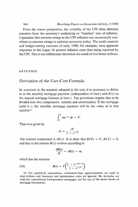
Derivation of the User-Cost Formula

IN ADDITION to the notation adopted in the text, it is necessary to define m as the monthly mortgage payment (independent of time) and B(t) as the unpaid mortgage balance at time t.. Tax provisions require that m be divided into two components: interest and amortization. If the mortgage yield is r, the monthly mortgage payment will be the value of m that satisfies23

rT

f me-rt dt = V.

Thus m is given by

rV m 1 e-rT

The interest component is rB(t). It is clear that B(0) V, B(T) 0, and that in the interim B(t) evolves according to

dB(t) = rB(t) -m, dit

which has the solution

0 B - e-r(T-t) (I10) B(t.)= Vt - _e-rT)

23. For analytical convenience, continuous-time approximations are used in what follows and insurance and maintenance costs are ignored. My formulas are valid for conventional level-payment mortgages, not for any of the newer forms of mortgage instruments.

Alan S. Blinder 565

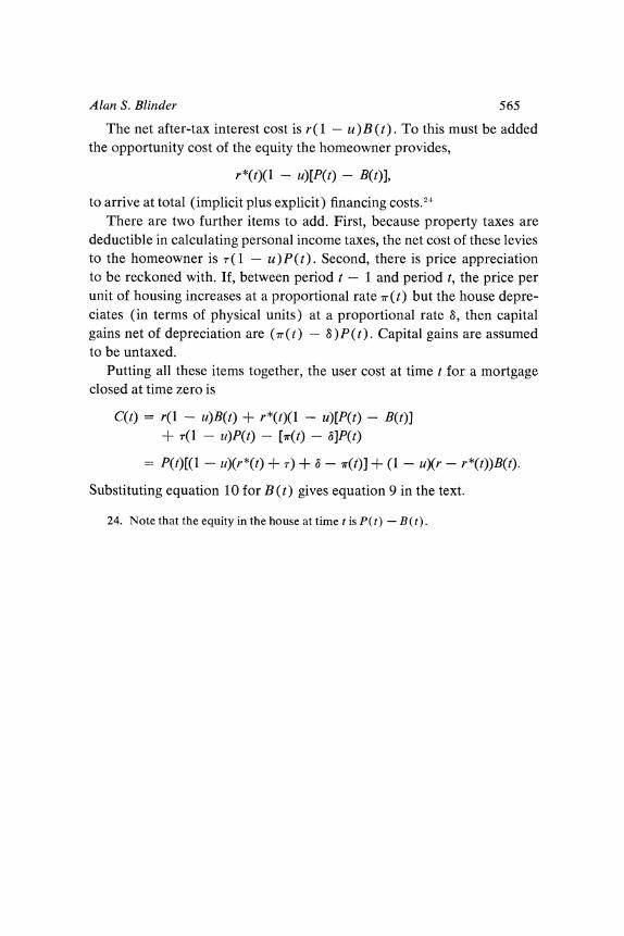
The net after-tax interest cost is r( 1 - u) B (t). To this must be added the opportunity cost of the equity the homeowner provides,

r*(t)(1- u)[P(t) -B(t)],

to arrive at total (implicit plus explicit) financing costs.24 There are two further items to add. First, because property taxes are

deductible in calculating personal income taxes, the net cost of these levies to the homeowner is Tr(1 - u)P(t ). Second, there is price appreciation to be reckoned with. If, between period t - 1 and period t., the price per unit of housing increases at a proportional rate 7(t.) but the house depre- ciates (in terms of physical units) at a proportional rate 8, then capital gains net of depreciation are (7(t) - 8)P(t.). Capital gains are assumed to be untaxed.

Putting all these items together, the user cost at time t. for a mortgage closed at time zero is

C(t) = r(1 - u)B(t) + r*(t)(l -u)[P(t) -B(t)] + r(1 - u)P(t) - [r(t) -b]P(t)

= P(t)[(l - ii)(r*(t) + r) + a - r(t)] + (1 - u)(r - r*(t))B(t).

Substituting equation 10 for B(t) gives equation 9 in the text.

24. Note that the equity in the house at time t is P(t) - B(t).

Comment by Jack E. Triplett

THE CPI and the implicit price deflator for personal consumption expenditure (PCE deflator, or just PCE) correspond, respectively, to Laspeyres and Paasche index number formulas. Moreover, the fact that these two formulas may give different measures of inflation is one of the oldest con- cerns in the theory of index numbers. However, as Blinder's paper em- phasizes, direct comparison of CPI and PCE measures does not yield a measure of the Paasche-Laspeyres discrepancy because the two indexes differ in many ways other than their formulas. The single biggest source of difference in recent quarters comes from the treatment of housing in the CPI, which Blinder analyzes at length.

To isolate the effect of different index formulas, I enlarge on Blinder's discussion of the three alternative versions of the PCE deflator regularly published by the Bureau of Economic Analysis.1 The implicit deflator itself is the Paasche index, which always takes its weights from the current quarter of the comparison-that is, every quarter a new set of weights is used to calculate the change in price from 1972 to the current quarter. A Laspeyres formula PCE, using 1972 weights, provides an alternative computation of the change between 1972 and the current period. This is commonly known as the "fixed-weight" price index for personal consumption; or, to be precise, the Laspeyres PCE, with 1972 weights. A third useful measure is the "chain price index"; this is another Laspeyres formula index, with the weights taken from the first of two quarters being

1. The current CPI weights come from the 1972-73 Consumer Expenditure Sur- vey, and no comparable data for a later period exist. For this reason, one cannot at present recompute the CPI for recent periods using the Paasche formula. The new Continuing Consumer Expenditure Survey program of the Bureau of Labor Statistics may permit CPI reweighting exercises to be carried out in the future. See Eva Jacobs, "Family expenditure data to be available on a continuing basis," Monthly Labor Review, vol. 102 (April 1979), pp. 53-54.

0007-2303/80/0002-0567$01.00/0 (? Brookings Institution

~~~~~~~L)Z~~~~~~~~~~~~~~~~)

00 2~~~~~~~~~~~ 00 00 tf)

0

0)0. 0) 0

00

\O N .O 06

0 --I

N. N - -- 0

-- .~~~~~~~0 00

O 0

t, ~ ~ ~ ~ ~ N 0 ()

06 06 CS * 0 0

~0 00

0)s 0)

U. 0~~~~~~. 0)

ON * N~~~~N ) '

C/ONO U 00 03C cn r~~- 7>0 16.~~~~~~~~~~~~~~~~~~~~~0

ON C~~~~~~~~~~oo N. ON ON ~~~~~ 0 M0)CZ

o .20~~~~c ..t Z~ '.0~~~~~~~

N. 0* >

Alan S. Blinder 569

compared (that is, the index of price change between, say, the second and third quarters of 1979 will have second-quarter 1979 weights). This index is referred to as the Laspeyres-chain index.

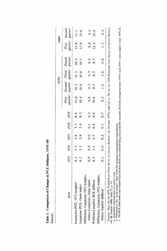
The Laspeyres PCE, 1972 weights, and Laspeyres-chain PCE index both use the same formula, differing only in the period to which the weights apply. Hence, comparing the two, as in the third row of table 1, provides an estimate of how updating the Laspeyres weights would affect the measured rate of current inflation. The two indexes were once very close together, but as the period between weights lengthens, they have diverged. For the first half of 1980 the divergence averages about half a percentage point, and the alternative inflation rates are about 121/2 percent for the fixed weight as compared to roughly 12 percent for the chain index. The difference between the two price measures is high by historical standards, but not sufficiently great to influence one's perception of the degree of inflation.

As shown in the fourth row of table 1, the change in the implicit PCE deflator has been lower than either of the Laspeyres versions, and this fact has frequently been taken to mean that the implicit PCE deflator is recording a lower rate of inflation than alternatives. This interpretation is incorrect because the change in that index has no clear meaning as a measure of inflation. A consideration of the implicit deflator formula and what is known about cost-of-living indexes will show this.

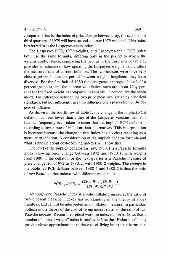
The level of the implicit deflator for, say, 1980: 1 is a Paasche formula index, showing price change between 1972 and 1980:1, with weights from 1980: 1; the deflator for the next quarter is a Paasche measure of price change from 1972 to 1980:2, with 1980:2 weights. The change in the published PCE deflator between 1980:1 and 1980:2 is thus the ratio of two Paasche price indexes with different weights, or

PCEt+1/IPCE, = Z +1W+ 1OW+1

+ I ~~(EPt wt /ZPo Wt)

Although one Paasche index is a valid inflation measure, the ratio of two different Paasche indexes has no standing in the theory of index numbers, and cannot be interpreted as an inflation measure. In particular, nothing in the theory of the cost-of-living index relates to the ratio of two Paasche indexes. Recent theoretical work on index numbers shows that a number of "mixed-weight" index formulas such as the "Fisher ideal" may provide closer approximations to the cost-of-living index than forms cur-

lb t-

- > z ? N IN a

D b xD O t I ,10 1-

E; 3,;E~~~~~~~--

bCi Ql. Q AS oSsQ~~~\

Alan S. Blinder 571

rently in use, but none of this work suggests that the ratio of two Paasche indexes is a desirable inflation measure.2

The correct comparison of inflation measures is, as already noted, shown in the third row of table 1 and not in the fifth row. The invalid comparison incorrectly suggests that, since early 1979, weights have been accounting for nearly a point on the annual inflation rate; the valid comparison shows that the difference is half that large.

The invalid comparison is the one that has often appeared in the press. Furthermore, many economists have evidently taken the "shifting weight" property of changes in the implicit PCE deflator as somehow providing a measure of the substitution bias inherent in any conventional fixed-weight price index.

As the Bureau of Economic Analysis' quarterly price index reconciliation table makes clear, the quarter-to-quarter change in the PCE deflator can be decomposed into a quantity-weighted price measure and a price- weighted quantity term.3 The price measure is the PCE "chain index," which, as noted above, is a Laspeyres index. The quantity index is a com- plex term that incorporates nearly all the economic changes affecting the consumption sector. Part of it is consumer substitution in response to relative price change; part is income-change effects on the budget shares of consumption goods; and part incorporates the effects of taste change and of everything else in the economy. The empirical question for inter- preting inflation measures is: how much of the "shifting weight" effect in the BEA's quarterly reconciliation table can be identified with the substitution error in a fixed-weight price index?4

This question cannot presently be answered for the current measures, but data for earlier years are suggestive. Consider the difference between the levels of the Paasche and Laspeyres indexes in table 2. The theory of index numbers tells us that part of the current difference of four points or so arises from a substitution error that infests both fixed-weight price indexes-that neither can take account of substitution in consumption

2. See especially W. Erwin Diewert, "Exact and Superlative Index Numbers," Journal of Econometrics, vol. 4 (May 1976), pp. 115-45.

3. For an example see Survey of Current Business, August 1980, p. 3. 4. Note that theory predicts that the sign of the substitution error must always be

the same-it is a bias relative to the true inflation measure. The signs of the shifting weight terms in Blinder's table 3 are frequently wrong, and the whole term has the wrong sign for 1978. Thus that term cannot be measuring the substitution error alone.


that occurs in response to relative price changes. Moreover, the theory states that when the substitution error is nonnegligible the Laspeyres index will be upward-biased because of consumer substitution and the Paasche index downward-biased, when both are used as approximations to a cost-of-living index. The theory also states that there are two cost-of- living indexes, one based on the reference period's indifference curve (here, 1972), the other referring to the indifference curve of the comparison period (here, any one of the periods tabulated in table 2).5

Thus that four-point 1980 Paasche-Laspeyres difference shown in table 2 can be partitioned into three parts-the substitution error in the fixed-weight Laspeyres relative to what I call the Laspeyres-perspective cost-of-living index; the substitution error in the fixed-weight Paasche index, relative to the analogous "Paasche-perspective" cost-of-living index; and the difference between the two cost-of-living indexes.

A study by Steven Braithwait confirms other suggestions that cost-of- living indexes based on different indifference curves can, and frequently do, give different measures. For example, Braithwait's estimated cost-of- living indexes computed for 1958 and 1970 indifference curves differ by about two percentage points over comparable time periods.6 This can be compared with an estimated substitution bias, over the 1958-73 period he studied, of only 1.5 percentage points.7

No one knows whether earlier estimates of the substitution bias, which have invariably found it quite small, will hold up in the current inflation. The degree of substitution bias depends, however, on the amount of relative price change-given substitution elasticities-and not just on the rate of inflation.

5. See Robert A. Pollak, "The Theory of the Cost of Living Index," Bureau of Labor Statistics, Working Paper 11 (June 1971), or Franklin M. Fisher and Karl Shell, The Economic Thleory of Price Itndices (Academic Press, 1972).

6. Steven D. Braithwait, "Consumer Demand and Cost of Living Indexes for the U.S.: An Empirical Comparison of Alternative Multi-Level Demand Systems," BLS Working Paper 45 (June 1975), table V.C., p. 30a.

7. Ibid., and Steven D. Braithwait, "The Substitution Bias of the Laspeyres Price Index: An Analysis Using Estimated Cost-of-Living Indexes," Americanl Econlomic Review (March 1980), table 2, p. 70.

Alan S. Blinder 573

Discussion

SOME discussants elaborated on the theoretical ambiguity inherent in defining a cost-of-living index. If used to deflate income, the appropriate construction depended on what concept of income it was meant to deflate. Edward Denison pointed out that, subject to the unavoidable index number problems, there is a price index that would answer the usual question for any specified measure of consumption: how much does current dollar consumption have to rise to hold constant dollar consumption unchanged? Joseph Pechman noted that this is the question implied in using the CPI to index retirement benefits and to index or otherwise inform wage and salary adjustments, and is also the way the CPI is interpreted in political debate and in public discussions of inflation. Although it would certainly make sense to alter the market basket of consumption in constructing the price index for social security retirees or for some other particular group, the main index ought to answer Denison's question for our best measure of consumption. The panel agreed that the current treatment of homeownership in the CPI is conceptually incorrect for deflating any realistic concept of consumption; and, in practice, it leads to far greater volatility in the CPI than a more appropriate measure would display.

Documents

The Consumer Price Index and the Measurement of … · ALAN S. BLINDER Princeton University and National Bureau of Economic Research The Consumer Price Index and the Measurement of