Embed Size (px)
Citation preview

The Conjecture of Birch and Swinnerton-Dyer
for elliptic curves with complex multiplication
by a nonmaximal order.
Thesis by
Jason Colwell
In Partial Fulfillment of the Requirements
for the Degree of
Doctor of Philosophy
California Institute of Technology
Pasadena, California
2004
(Defended 18 November 2003)

ii
c© 2004
Jason Colwell
All Rights Reserved

iii
Acknowledgements
First, I would like to thank my advisor, Matthias Flach, for his instruction
during my graduate studies, including his suggestion of this topic, and his help
in the writing of this thesis. I am grateful to the Department of Mathematics
at Caltech for providing a congenial environment for study and research. I
would like to thank my father and mother for their support and encouragement
throughout my doctoral program. Finally, I would like to thank my girlfriend,
Charlene, for her constant encouragement and personal support during the
writing of this thesis.

iv
Abstract
The Conjecture of Birch and Swinnerton-Dyer relates an analytic invariant of
an elliptic curve – the value of the L-function, to an algebraic invariant of
the curve – the order of the Tate–Safarevic group. Gross has refined the
Birch–Swinnerton-Dyer Conjecture in the case of an elliptic curve with com-
plex multiplication by the full ring of integers in a quadratic imaginary field.
It is this version which interests us here. Gross’ Conjecture has been refor-
mulated, by Fontaine and Perrin-Riou, in the language of derived categories
and determinants of perfect complexes. Burns and Flach then realized that
this immediately leads to a refined conjecture for elliptic curves with complex
multiplication by a nonmaximal order. The conjecture is now expressed as
a statement concerning a generator of the image of a map of 1-dimensional
modules. We prove this conjecture of Burns and Flach.
v
Contents
Acknowledgements iii
Abstract iv
0 Introduction. 1
1 The conjecture of Birch and Swinnerton-Dyer. 5
2 The Weil restriction. 9
3 The conjecture of Gross. 12
3.1 Choice of bases. . . . . . . . . . . . . . . . . . . . . . . . . . . 14
3.2 The conjecture. . . . . . . . . . . . . . . . . . . . . . . . . . . 16
4 The language of perfect complexes. 18
4.1 Determinants of perfect complexes. . . . . . . . . . . . . . . . 18
4.2 The setting. . . . . . . . . . . . . . . . . . . . . . . . . . . . . 22
4.3 Four vector spaces. . . . . . . . . . . . . . . . . . . . . . . . . 22
4.4 Galois cohomology. . . . . . . . . . . . . . . . . . . . . . . . . 23
4.5 Reformulation of Gross’ Conjecture. . . . . . . . . . . . . . . . 29
5 Elliptic curves with nonmaximal endomorphism ring. 47

vi
5.1 The Burns–Flach Conjecture. . . . . . . . . . . . . . . . . . . 52
5.2 A refinement in the case F (Etors)/K is abelian. . . . . . . . . 53
6 Translation into the terminology of Kato. 59
7 Proof of the conjecture. 68
7.1 A universal situation. . . . . . . . . . . . . . . . . . . . . . . . 68
7.2 The strategy of proof. . . . . . . . . . . . . . . . . . . . . . . 74
8 A Λ∞-basis of ∆Λ∞(OK,S,F∞). 76
9 The image of the basis. 86
10 Examples. 92
10.1 Elliptic curves with rank 0. . . . . . . . . . . . . . . . . . . . . 93
10.2 Elliptic curves with complex multiplication by a nonmaximal
order. . . . . . . . . . . . . . . . . . . . . . . . . . . . . . . . 93
10.3 A first attempt. . . . . . . . . . . . . . . . . . . . . . . . . . . 99
10.4 A second search. . . . . . . . . . . . . . . . . . . . . . . . . . 103
10.5 The code. . . . . . . . . . . . . . . . . . . . . . . . . . . . . . 105
Bibliography 119

1
Chapter 0
Introduction.
The Conjecture of Birch and Swinnerton-Dyer relates an analytic invariant of
an elliptic curve – the value of the L-function, to an algebraic invariant of
the curve – the order of the Tate–Safarevic group.
In our situation, the elliptic curve E is defined over a number field F .
The L-function, like the classical Riemann zeta function, is defined as a prod-
uct over prime ideals of F . The Tate–Shavarevich group is the group of 1-
cohomology classes of E which are locally trivial at each place of F .
For most elliptic curves E, the ring of endomorphisms End(E) is isomorphic
to Z. However, there are some elliptic curves whose endomorphism ring is
larger. In this case, E is said to have complex multiplication. It is elliptic
curves with this additional structure which interest us here. The basic theory
of the subject shows that if E has complex multiplication, then End(E) is
isomorphic to an order O in a quadratic imaginary field K.
Gross has refined the Birch–Swinnerton-Dyer Conjecture in the case where
O is the full ring of integers OK . It is this version which interests us here.
He uses the fact that the L-function of an elliptic curve with complex mul-

2
tiplication agrees with the product of two L-functions of a Grossencharacter
of F , associated to E, with values in K. Gross’ idea is to consider the two
L-functions separately, making a conjecture about each, viewing it as the K-
equivariant L-function. He formulates a complex regulator in place of the real
regulator used in the original conjecture. As well, he uses the order ideal of a
group in place of the cardinality of the group.
Rubin has proved the p-part of Gross’ conjecture in the case where F = K
(i.e., the class number of K is 1) and p does not divide |µOK | (the number
of roots of unity in K), under the condition rank(E(F )) = 0. Some cases of
Gross conjecture with F 6= K will follow from our results below.
Gross’ Conjecture has been reformulated, by Fontaine and Perrin-Riou,
in the language of derived categories and determinants of perfect complexes.
Burns and Flach then realized that this immediately leads to a conjecture
which is a refinement in the case where O 6= OK . The conjecture is now
expressed as a statement concerning a generator of the image of a map of 1-
dimensional modules. We wish to prove the p-part of this conjecture of Burns
and Flach for elliptic curves with complex multiplication by a nonmaximal
order, i.e., where O 6= OK , and where necessarily F 6= K. We shall use
Rubin’s restrictions
rank(E(F )) = 0
F (Etors)/K is abelian
p 6 | |µOH |
3
(H being the Hilbert Class field of K). In fact we shall also assume for sim-
plicity that K has class number 1 (i.e., H = K).
The formulation of Burns–Flach naturally allows a further refinement of
the conjecture, dealing with the Weil restriction B of E, and considering Rp-
modules in place of Op-modules, where R = End(B). (The conjecture will be
over the endomorphism algebra R of B, which is much larger than K.) We
shall prove this conjecture by reducing it to the Main Conjecture for imaginary
quadratic fields. At this point we need to make the further assumption that
p 6 | [K f0p : K],
where f0 is the prime-to-p part of the conductor of B and Km/K denotes the
ray class field of conductor m, because Rubin’s proof of the Main Conjecture
requires this condition.
We shall use a method of Kato to address this situation, first dualizing
the modules involved, then passing to a situation universal with respect to
invertible sheaves over p-adic rings. The conjecture is then seen to follow from
two known results, the Explicit Reciprocity Law and Rubin’s Main Conjecture.
We first discuss the conjectures which are ancestors of the Burns–Flach
Conjecture under consideration, and the translation between the language of
the original Birch–Swinnerton-Dyer Conjecture and that of perfect complexes.
Next, a deduction of the Burns–Flach Conjecture, from the Main Conjecture
and the Explicit Reciprocity Law, is given. Finally, we discuss numerical
examples of the conjectures.

4
5
Chapter 1
The conjecture of Birch andSwinnerton-Dyer.
We will give the Birch–Swinnerton-Dyer Conjecture in its original generality,
applying not only to elliptic curves but to abelian varieties in general. We
follow [9] in our exposition.
Let A be an abelian variety of dimension g which is defined over a number
field F .
Write L(A/F, s) for the L-series of A over F , which is defined by the Euler
product
L(A/F, s) =∏w 6 |∞
Pw(A/F,Nw−s)−1,
where for any finite place w of F
Pw(A/F, x) := det(1− xφw | (T`(A)⊗Q`)Iw),
the characteristic polynomial of the action of Frobenius (φw) upon the inertia
`-adic Tate quotient module (T`(A)⊗Q`)Iw (which is the co-invariants, under
the action of the inertia group Iw, of the `-adic Tate module T`(A) ⊗ Q`).

6
This polynomial is independent of ` and has coefficients in Z. The L-series is
convergent in the half-plane s ∈ C : Re(s) > 32.
Let III(A) be the Tate-Safarevic group
ker
(H1(F,A)→
∏w
H1(Fw, A)
)
of A over F . (The product is taken over all places w of F .) The following is
conjectured to be true, and will be assumed here.
Assumption 1.0.1. III(A) is finite.
A constant is defined using the Neron model, the invariant differentials on
A and their period integrals, and the discriminant of F/Q. The constant will
be conjecturally related to the L-function.
Write A for the Neron model of A, and Aw = A⊗OF kw after a base change
to the residue field of F at a finite place w. Write A0w for the connected
component of the origin in Aw.
Let (ω1, . . . , ωg) be an F -basis of H0(A,ΩA/F ). Denote the projective OF -
module of invariant differentials on the Neron model A of A, by ΩA. Then∧g ΩA, restricted to H0(A,ΩgA/F ), is given by
(g∧i=1
ωi
)·D
for some fractional ideal D of OF .
For a complex place w of F , let (h1, . . . , h2g) be a Z-basis of the integral

7
homology H1(A(Fw),Z). Define
Ωw :=
∣∣∣∣det
(∫hi
ωj
∣∣∣∣∫hi
ωj
)∣∣∣∣ .This is non-zero and depends only on
∧gi=1 ωi and w.
For a real place w of F , corresponding to the embedding σ : F → R,
let (h1, . . . , hg) be a Z-basis of H1(A(Fw),Z)+, the submodule of the integral
homology H1(A(Fw),Z) fixed by complex conjugation. Define
Ωw :=
∣∣∣∣ Aσ(R)
Aσ(R)0
∣∣∣∣ · ∣∣∣∣det
(∫hi
ωj
)∣∣∣∣ .This is non-zero and depends only on
∧gi=1 ωi and w.
Fix bases (x1, . . . , xn) and (y1, . . . , yn) of respective free subgroups X ⊂
A(F ) and Y ⊂ A(F )∨ of finite index. (Here ∨ indicates the dual abelian
variety.) Define the regulator
R :=| det(< xi, yj >)|∣∣∣A(F )
X
∣∣∣ · ∣∣∣A∨(F )Y
∣∣∣ ,where <,> is the canonical height pairing corresponding to the Poincare di-
visor on A × A∨. The value of R ∈ R∗ is independent of X and Y and their
bases.
Now we are ready to state the conjecture of Birch and Swinnerton-Dyer:
Conjecture 1.0.2 (Birch–Swinnerton-Dyer). We have
L(A/F, s) ∼ c(s− 1)rankZA(F ) as s→ 1

8
for some constant c ∈ R∗+ such that
c
R ·∏
w|∞ Ωw
lies in Q and equals
|discF/K |−g/2 ·NF/QD · |III(A)| ·∏w 6 |∞
∣∣∣∣Aw(kw)
A0w(kw)
∣∣∣∣ .Note that the last product is well-defined because for all but the finite
number of places w of bad reduction, we have Aw(kw) = A0w(kw), and the
multiplicand equal to 1.
We are interested in the case where rankZA(F ) = 0, whereupon the asser-
tion of the conjecture reduces to
L(A/F, 1) · |A(F )| · |A∨(F )|∏w|∞ Ωw
= |discF/K |−g/2·NF/QD·|III(A)|·∏w 6 |∞
∣∣∣∣Aw(kw)
A0w(kw)
∣∣∣∣ ∈ Q.

9
Chapter 2
The Weil restriction.
To discuss Gross’ refinement of the Birch–Swinnerton-Dyer Conjecture, we
will need the Weil restriction. Let A be abelian variety defined over F , an
extension of a number field K. The Weil restriction
B := ResFKA
is an abelian variety defined over K, whose construction we recall now.
For simplicity assume that F/K is Galois.
For each element σ of G := Gal(F/K), we have a commutative diagram of
schemes
A
Aσ
σoo
Spec(F )
&&MMMMMMMMMMSpec(F )
xxqqqqqqqqqq
σoo
Spec(K)
,

10
where Aσ is the fibre product of
A
Spec(F ) Spec(F ).σoo
Taking the fibre product over all σ, we have
B :=∏
σ∈GAσ
Spec(F )
Spec(K).
The finite group G acts on the projective scheme B, compatibly with its action
on F . Therefore, there exists a scheme B which is the quotient of B by the
G-action. B is then defined over K. This variety B is abelian, with the group
law inherited from A via B. It is seen that B satisfies the desired functorial
property:
Lemma 2.0.1. B is a K-variety such that
HomSpec(K)(Y,B) ' HomSpec(F )(Y ⊗K F,A)
for any K-scheme Y . (The functor ResFK is the right adjoint of the extension-
of-scalars functor Y 7→ Y ⊗K F . ) In particular, for Y = Spec(C) and a

11
complex place v of K, we have
B(C) = HomSpec(K)(Spec(C), B) ' HomSpec(F )(Spec(C⊗KF ), A) =⊕w|v
A(Fw).
If A is an elliptic curve with complex multiplication by an order O in an imagi-
nary quadratic field K, this equality of functors provides B with multiplication
by (at least) O.
12
Chapter 3
The conjecture of Gross.
Gross has refined (in [9]) the conjecture of Birch–Swinnerton-Dyer for elliptic
curves with complex multiplication.
Let E be an elliptic curve defined over a number field F , with complex
multiplication by the ring of integers OK of a quadratic imaginary field K. If
we fix an isomorphism OK ' EndF (E), then the action of EndF (E) on Lie(E)
gives an embedding K → F . If we fix a complex embedding K → C, we
obtain a Grossencharacter ψ of F with values in C∗. See [21], II, §9.
We replace the Q`-action on the `-adic Tate module T`(E) ⊗ Q` by the
K⊗Q`-action given by complex multiplication. Now the global K-equivariant
L-series of E/F is defined
KL(E/F, s) :=∏w 6 |∞
KPw(E/F,Nw−s)−1,
where
KPw(E/F, x) = detK⊗Q`
(1− xφw | (T`(E)⊗Q`)Iw),

13
the characteristic polynomial of the action of Frobenius (φw) upon the inertia
`-adic Tate quotient module (T`(A) ⊗ Q`)Iw . The product is over all finite
primes of F .
On the other hand, we have the Hecke L-series
L(ψ, s) :=∏
w 6 |∞·fψ
(1− ψ(w)Nw−s)−1.
(The product is over the finite primes of F not dividing the conductor fψ of
ψ.) This product is convergent in the half-plane s ∈ C : Re(s) > 32 and has
an analytic continuation to the entire plane by Hecke. (See [21], II, §10.)
It is known, by a theorem of Deuring, that
KL(E/F, s) = L(ψ, s).
Hence we also have
L(E/F, s) = L(ψ, s)L(ψ, s),
reflecting the identity of Euler factors NK/Q(KPw(x)) = Pw(x). The aim of
Gross’ Conjecture is to identify the leading term of L(ψ, s) instead of that of
L(E/F, s) (whose leading term is the subject of the Birch–Swinnerton-Dyer
Conjecture).
14
3.1 Choice of bases.
We continue to write B = ResFKE for the Weil restriction of E. The [F : K]-
dimensional abelian variety B is canonically self-dual and has complex multi-
plication by OK . We have
KL(B/K, s) = KL(E/F, s).
As before, a “constant” is defined using the Neron model, the invariant differ-
entials on E, and their period integrals. But this time, the “constant” is an
ideal in OK . This ideal will again be conjecturally related to the L-function.
Write B for the Neron model of B, and Bv = B⊗OK kv after a base change
to the residue field of K at a finite place v. Write B0v for the connected
component of the origin in Bv.
Let (ω1, . . . , ω[F :K]) be an K-basis of H0(B,ΩB/K). Denote the projective
OK-module of invariant differentials on the Neron model B of B, by ΩB. Then∧[F :K] ΩB, restricted to H0(B,Ω[F :K]B/K ), is given by
[F :K]∧i=1
ωi
· dfor some fractional ideal d of OK .
The integral homology H1(B(C),Z) is a projective OK-module of rank
[F : K]. Let (h1, . . . , h[F :K]) be a K-basis of H1(B(C),Q). Then
∧[F :K]OK
H1(B(C),Z)
15
is given by [F :K]∧j=1
hj
· bfor some fractional ideal b of OK . Let (γ1, . . . , γ[F :K]) be the dual K-basis of
H1(B(C),Q). Then ∧[F :K]OK
H1(B(C),Z)
is given by [F :K]∧j=1
γj
· b−1.
Define
Ω := det
(∫hi
ωj
).
This is non-zero.
Fix a basis (x1, . . . , xn) of a free OK-submodule X ⊂ B(K) of finite index.
Define the complex regulator
RC :=det(< xi, xj >C)∣∣∣B(K)
X
∣∣∣ ,
where
<,>: B(K)×B(K)→ R
16
is the height pairing and
<,>C: B(K)×B(K)→ C
is
(x, y) 7→ δ < x, y > − < x, δy >,
1, δ being a Z-basis of OK , and <,>C is independent of the choice of δ. The
value of RC ∈ C∗ is independent of X and its basis.
3.2 The conjecture.
Let “#” denote the order ideal as an OK-module.
Now we can state Gross’ refinement of the Birch–Swinnerton-Dyer Conjec-
ture.
Conjecture 3.2.1 (Gross). We have
L(ψ, s) ∼ c(s− 1)rankOKB(K) as s→ 1
for some constant c ∈ C∗ such that
c
RCΩ

17
lies in K and generates
b · d ·#(III(B)) ·∏w 6 |∞
#
(Bv(kv)
B0v(kv)
).
We are interested in the case where rankOKB(K) = 0, whereupon the
assertion of the conjecture reduces to
(L(ψ, s) · |B(K)|
Ω
)= b · d ·#(III(B)) ·
∏w 6 |∞
#
(Bv(kv)
B0v(kv)
).
As explained by Gross, we have
NL(ψ, s) =L(B/K, s),
NRC =R,
N(Ω) =∏w|∞
Ωw
Nb =|discF/K |g/2
Nd =NF/QD
N(#III(B)) =|III(E)|
N
∏w 6 |∞
#
(Bv(kv)
B0v(kv)
) =∏v 6 |∞
∣∣∣∣Bv(kv)
B0v(kv)
∣∣∣∣ .(the first three norms being the complex norm z 7→ zz, the others being the
norm map on ideals) so that the original Birch–Swinnerton-Dyer Conjecture
follows from Gross’ Conjecture.
18
Chapter 4
The language of perfectcomplexes.
In this chapter we reformulate Gross’ Conjecture using the language of perfect
complexes and their determinants, essentially following Fontaine and Perrin-
Riou in [6].
4.1 Determinants of perfect complexes.
By a complex we mean a sequence of modules M jj∈Z over some ring, say
Q, indexed by the integers, with maps
M jdj //M j+1
satisfying dj+1 dj = 0 for all j ∈ Z.
By a perfect complex we mean a complex which is quasi-isomorphic to
a bounded complex whose terms are finite projective modules. (These are the
complexes for which it will be possible to define the determinant.)
The determinant of a perfect complex is the alternating tensor product
19
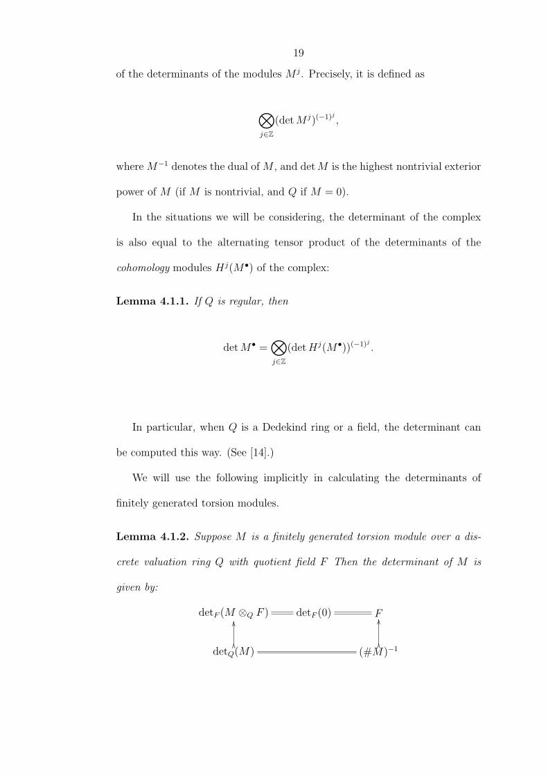
of the determinants of the modules M j. Precisely, it is defined as
⊗j∈Z
(detM j)(−1)j ,
where M−1 denotes the dual of M , and detM is the highest nontrivial exterior
power of M (if M is nontrivial, and Q if M = 0).
In the situations we will be considering, the determinant of the complex
is also equal to the alternating tensor product of the determinants of the
cohomology modules Hj(M•) of the complex:
Lemma 4.1.1. If Q is regular, then
detM• =⊗j∈Z
(detHj(M•))(−1)j .
In particular, when Q is a Dedekind ring or a field, the determinant can
be computed this way. (See [14].)
We will use the following implicitly in calculating the determinants of
finitely generated torsion modules.
Lemma 4.1.2. Suppose M is a finitely generated torsion module over a dis-
crete valuation ring Q with quotient field F Then the determinant of M is
given by:
detF (M ⊗Q F ) detF (0) F
detQ(M)OO
OO
(#M)−1OO
OO

20
Proof. Write additively the group operation of M . Let x1, . . . , xn be gen-
erators of M , and M ′ the free module on those generators. Let M ′′ be the
kernel of M ′ η→M , a submodule of M ′ (also free) whose generators we denote
by y1, . . . , yn. Denoting by d : M ′′ →M ′ the inclusion, we have
d(y1) = a11x1 + · · ·+ a1nxn,
d(y2) = a21x1 + · · ·+ a2nxn,
...
d(yn) = an1x1 + · · ·+ annxn,
for some ajk ∈ Q, j, k = 1, . . . , n. Then M has the finite projective resolution
· · · // 0 //M ′′ //M ′ //M // 0 // · · · ,
concentrated in degrees -1 and 0. So detM = detM ′ ⊗ det−1M ′′. Over F , d
induces the isomorphism
M ′′ ⊗Q F 'd
//M ′ ⊗Q F .
We wish to identify the invertible Q-module
detM ′ ⊗Q (detM ′′)−1

21
inside the invertible F -module
(detF
(M ′ ⊗Q F ))⊗F
(detF
(M ′′ ⊗Q F ))−1
.
Now (detF
(M ′ ⊗Q F ))⊗F
(detF
(M ′′ ⊗Q F ))−1
has canonical basis
d(y1) ∧ · · · ∧ d(yn)⊗ (y1 ∧ · · · ∧ yn)−1
while
detM ′ ⊗Q (detM ′′)−1
has canonical basis
det(ajk)−1 · d(y1) ∧ · · · ∧ d(yn)⊗ (y1 ∧ · · · ∧ yn)−1.
We have the diagram
η(y1) ∧ · · · ∧ η(yn)⊗ (y1 ∧ · · · ∧ yn)−1 //
∈
1
∈
(detF (M ′ ⊗Q F ))⊗F (detF (M ′′ ⊗Q F ))−1 ' // F
detM ′ ⊗Q (detM ′′)−1 ' //OO
OO
Q · det(ajk)−1
OO
OO
det(ajk)−1 · η(y1) ∧ · · · ∧ η(yn)⊗ (y1 ∧ · · · ∧ yn)−1 //
∈
det(ajk)−1,
∈

22
where the isomorphisms are induced by d. As Q is a DVR, det(ajk) ·Q = #M .
The result follows.
4.2 The setting.
Let B be an abelian variety defined over the quadratic imaginary field K,
and so that there is an embedding OK → EndK(B). Denote by B∨ the dual
abelian variety.
The situation we have in mind is that in which B is the Weil restriction
of an elliptic curve with complex muliplication by OK . Here we would have
B ' B∨. We make the same assumption about the Tate–Safarevic group as
before:
Assumption 4.2.1. III(B) is finite.
Fix K → C.
4.3 Four vector spaces.
We have four finite-dimensional K-vector spaces H0(B,Ω1), H1(B(C),Q),
B(K)⊗Z Q, B∨(K)⊗Z Q and perfect K ⊗ R = C-linear pairings
(H0(B,Ω1B/K)⊗Q R)× (H1(B(C),Q)⊗Q R)→ C (4.1)
induced by integration and
(B(K)⊗Z R)× (B∨(K)c ⊗Z R)→ C (4.2)

23
given by the modified height pairing <,>C discussed earlier. (For any K-
module W we denote by W c the same group W with the conjugate action of
K.) Defining
KΞ := detKH0(B,Ω1
B/K)⊗K detKH1(B(C),Q)
⊗K (detKB(K)⊗Z Q)⊗K (det
KB∨(K)c ⊗Z Q),
these pairings induce a K ⊗ R = C-linear isomorphism
Kϑ∞ : KΞ⊗Q R ' K ⊗ R.
4.4 Galois cohomology.
We fix a prime number p, and a finite set S of places of K, containing the
infinite place, those places above p, and all places where B has bad reduction.
We denote by GS the Galois group of the maximal extension of K unramified
outside S and by OK,S the ring of S-integers of K. For any continuous GS-
module N we put
RΓ(OK,S, N) = C•(GS, N),
the standard complex of continuous cochains. We define
RΓc(OK,S, N)
=Cone
(RΓ(OK,S, N)→
⊕v∈S
RΓ(Kv, N)
)[−1].

24
Suppose v 6 | p is a place of K. Define
RΓf(Kv, Vp(B))
to be the perfect complex, concentrated in degrees 0 and 1, of K⊗Qp-modules
· · · // 0 // Vp(B)Iv1−Frobv// Vp(B)Iv // 0 // · · · . (4.3)
Define
RΓf(Kv, Tp(B))
to be the complex
B(Kv)[−1],
which is
· · · // 0 // B(Kv)// 0 // · · · , (4.4)
concentrated in degree 1, where B(Kv) := lim←−n
B(Kv)/pn is the p-completion of
B(Kv).
For v | p, we define
RΓf(Kv, Vp(B))
to be the perfect complex, concentrated in degrees 0 and 1, of K⊗Qp-modules
· · · // 0 // Dv
(1−φ,π) // Dv ⊕H0(B,Ω1B/Kv
)∨ // 0 // · · · , (4.5)
25
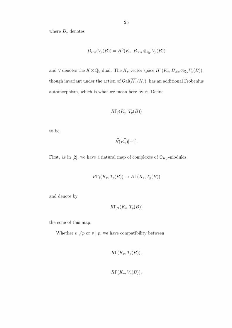
where Dv denotes
Dcris(Vp(B)) = H0(Kv, Bcris ⊗Qp Vp(B))
and ∨ denotes the K⊗Qp-dual. The Kv-vector space H0(Kv, Bcris⊗Qp Vp(B)),
though invariant under the action of Gal(Kv/Kv), has an additional Frobenius
automorphism, which is what we mean here by φ. Define
RΓf(Kv, Tp(B))
to be
B(Kv)[−1].
First, as in [2], we have a natural map of complexes of OK,p-modules
RΓf(Kv, Tp(B))→ RΓ(Kv, Tp(B))
and denote by
RΓ/f(Kv, Tp(B))
the cone of this map.
Whether v 6 | p or v | p, we have compatibility between
RΓ(Kv, Tp(B)),
RΓ(Kv, Vp(B)),

26
and the natural map
RΓf(Kv, Tp(B))→ RΓ(Kv, Tp(B)),
as follows. If v 6 | p, then
RΓ(Kv, Tp(B))⊗Zp Qp = B0(Kv)[−1]⊗Zp Qp
is the zero complex, which is quasi-isomorphic to
RΓ(Kv, Vp(B)).
If v | p, we have
RΓf(Kv, Tp(B))⊗Zp Qp = B(Kv)⊗Zp Qp[−1],
which is quasi-isomorphic to the complex
RΓf(Kv, Vp(B)),
via the exponential map
H0(B,ΩBv)∨
exp' // B(Kv)⊗Zp Qp
in degree 1.

27
Remark 4.4.1. If B has good reduction at v 6 | p, then
RΓf(Kv, Tp(B))
could have been defined as was
RΓf(Kv, Vp(B))
to obtain the same cohomology. Precisely,
RΓf(Kv, Tp(B)) = B(Kv) = B0(Kv)
is quasi-isomorphic to the complex
· · · // 0 // Tp(B)Iv1−Frobv// Tp(B)Iv // 0 // · · · , (4.6)
concentrated in degrees 0 and 1, which lies inside
RΓf(Kv, Vp(B)).
The quasi-isomorphism is compatible with the natural map
RΓf(Kv, Tp(B))→ RΓ(Kv, Tp(B)),
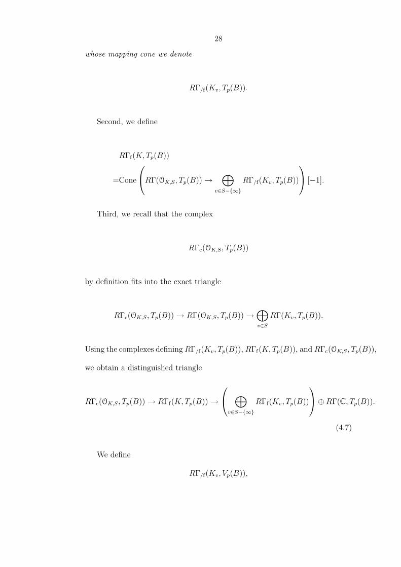
28
whose mapping cone we denote
RΓ/f(Kv, Tp(B)).
Second, we define
RΓf(K,Tp(B))
=Cone
RΓ(OK,S, Tp(B))→⊕
v∈S−∞
RΓ/f(Kv, Tp(B))
[−1].
Third, we recall that the complex
RΓc(OK,S, Tp(B))
by definition fits into the exact triangle
RΓc(OK,S, Tp(B))→ RΓ(OK,S, Tp(B))→⊕v∈S
RΓ(Kv, Tp(B)).
Using the complexes definingRΓ/f(Kv, Tp(B)), RΓf(K,Tp(B)), andRΓc(OK,S, Tp(B)),
we obtain a distinguished triangle
RΓc(OK,S, Tp(B))→ RΓf(K,Tp(B))→
⊕v∈S−∞
RΓf(Kv, Tp(B))
⊕RΓ(C, Tp(B)).
(4.7)
We define
RΓ/f(Kv, Vp(B)),

29
RΓf(K,Vp(B)),
RΓc(OK,S, Vp(B)),
similarly. There is a version of triangle (4.7) with rational (Vp(B)) coefficients,
and we have
RΓc(OK,S, Tp(B))⊗Zp Qp ' RΓc(OK,S, Vp(B)).
Here, since we are dealing with the regular rings K, K⊗Qp, and OK ⊗Zp,
the determinants of the complexes considered are alternating tensor products
of the determinants of the cohomology modules, as noted in Chapter 4.1.
4.5 Reformulation of Gross’ Conjecture.
In order to reformulate Gross’ Conjecture, we wish to relate #(III(B)p∞) to
the determinant of
RΓc(OK,S, Tp(B)),
viewed as an integral lattice inside the determinant of
RΓc(OK,S, Vp(B)).
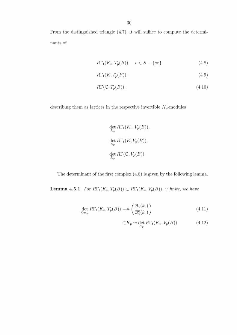
30
From the distinguished triangle (4.7), it will suffice to compute the determi-
nants of
RΓf(Kv, Tp(B)), v ∈ S − ∞ (4.8)
RΓf(K,Tp(B)), (4.9)
RΓ(C, Tp(B)), (4.10)
describing them as lattices in the respective invertible Kp-modules
detKp
RΓf(Kv, Vp(B)),
detKp
RΓf(K,Vp(B)),
detKp
RΓ(C, Vp(B)).
The determinant of the first complex (4.8) is given by the following lemma.
Lemma 4.5.1. For RΓf(Kv, Tp(B)) ⊂ RΓf(Kv, Vp(B)), v finite, we have
detOK,p
RΓf(Kv, Tp(B)) =#
(Bv(kv)
B0v(kv)
)(4.11)
⊂Kp ' detKp
RΓf(Kv, Vp(B)) (4.12)

31
if v 6 | p, and
(4.13)
detOK,p
RΓf(Kv, Tp(B)) =d ·#(
Bv(kv)
B0v(kv)
)·
[F :K]∧j=1
ωj
(4.14)
⊂Kp ·
[F :K]∧j=1
ωj
' detKp
RΓf(Kv, Vp(B)) (4.15)
if v | p. Here the isomorphisms are induced by maps between cohomology in
degrees 0 and 1.
For the proof of the lemma we use the following two results, The first is
from Lemma 1 of [3], and the second is proved using [11].
Lemma 4.5.2. Suppose
· · · // 0 //Mη //M // 0 // · · · ,
is a complex of finite projective Q-modules, concentrated in degrees 0 and 1.
Then there is a commutative diagram
det(Q) det(M)⊗ det(M)−1 ' //
Lemma 4.1.1
Q
det(η)
detQH0(M)⊗ detQH
1(M)−1
detQ(0)⊗ detQ(0)−1 Q
where the horizontal isomorphism is induced by idM .

32
Lemma 4.5.3.
B(Kv)/H1(kv, Tp(B)Iv) ' Bv(kv)/B
0(kv).
Proof. We denote by B the Neron model of B/Kv, by B0 the zero connected
component subscheme, by Bv the special fibre, and by B0v the zero connected
component of Bv. By [11], Lemma 2.2.1, there is a short exact sequence of
group schemes
0 // B0pn
// B0pn // B0 // 0 .
We also use the short exact sequence of group schemes
0 // Bpn// B
pn // B // 0 .
From these exact sequences for B0 and B, we obtain the exact sequences
B(Kv)pnpn // B(Kv)pn // H1(Kv,Bpn) ,
B0(OK,v)pnpn // B0(OK,v)pn // H1(OK,v,B
0pn) ,
B0v(kv)pn
pn // B0v(kv)pn
// H1(kv, (B0v)pn) ,
which induce respective injections
B(OK,v)pn B(Kv)pn // // H1(Kv,Bpn) H1(Kv, Bpn) ,
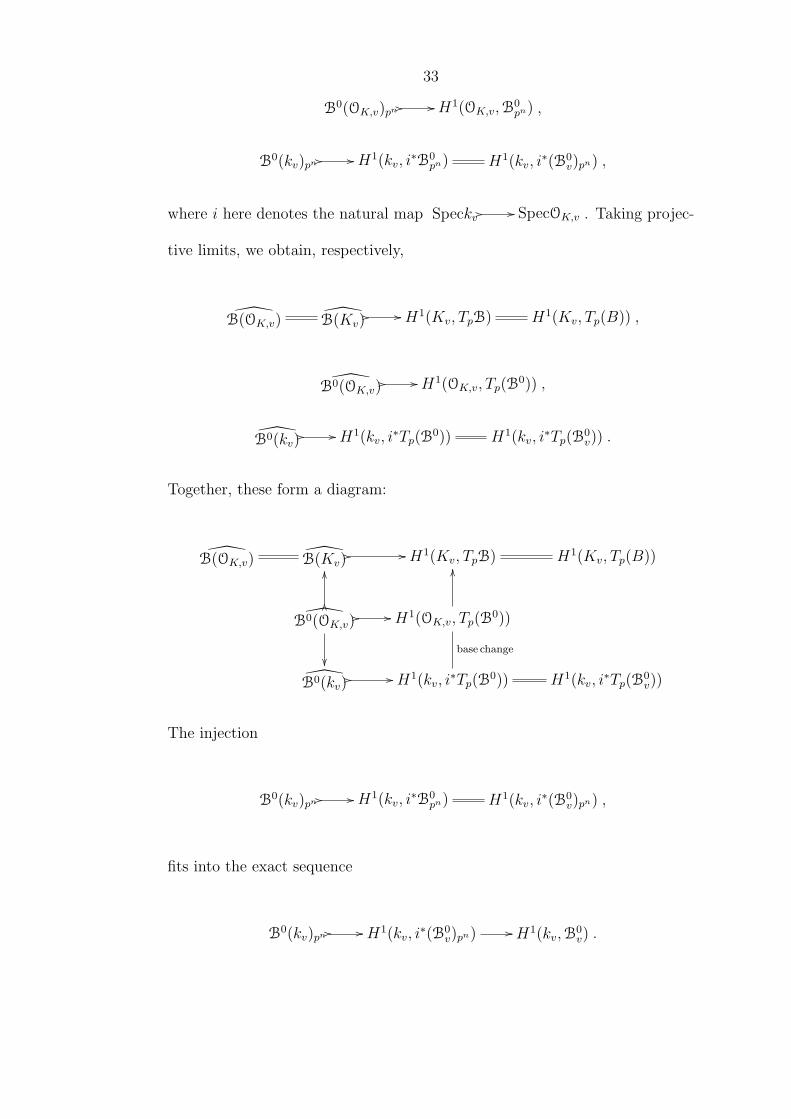
33
B0(OK,v)pn // // H1(OK,v,B0pn) ,
B0(kv)pn // // H1(kv, i∗B0
pn) H1(kv, i∗(B0
v)pn) ,
where i here denotes the natural map Speckv // // SpecOK,v . Taking projec-
tive limits, we obtain, respectively,
B(OK,v) B(Kv)// // H1(Kv, TpB) H1(Kv, Tp(B)) ,
B0(OK,v)// // H1(OK,v, Tp(B
0)) ,
B0(kv)// // H1(kv, i
∗Tp(B0)) H1(kv, i
∗Tp(B0v)) .
Together, these form a diagram:
B(OK,v) B(Kv)// // H1(Kv, TpB) H1(Kv, Tp(B))
B0(OK,v)// //
OO
OO
H1(OK,v, Tp(B0))
base change
OO
B0(kv)// // H1(kv, i
∗Tp(B0)) H1(kv, i
∗Tp(B0v))
The injection
B0(kv)pn // // H1(kv, i∗B0
pn) H1(kv, i∗(B0
v)pn) ,
fits into the exact sequence
B0(kv)pn // // H1(kv, i∗(B0
v)pn)// H1(kv,B
0v) .

34
By Lang’s Theorem H1(kv,B0v) = 0, so that the map
B0(kv)pn // // H1(kv, i∗B0
pn) H1(kv, i∗(B0
v)pn) .
is surjective. By [11], Proposition 2.2.5, we have
H1(kv, i∗Tp(B
0v)) = H1(kv, (Tp(B
0))Iv),
The map
B0(OK,v)→ B0(kv)
is surjective since A0 → OK,v is smooth and OK,v Henselian, injective since
v 6 | p, making ker(B0(OK,v)→ B0(kv)) p-divisible. Since Speckv is proper over
SpecOK,v, then
H1(OK,v, Tp(B0)) ' H1(kv, i
∗Tp(B0)).
We obtain this diagram:
B(OK,v) B(Kv)// // H1(Kv, TpB) H1(Kv, Tp(B))
B0(OK,v)// //
OO
OO
H1(OK,v, Tp(B0))
'
OO
B0(kv)// // // H1(kv, i
∗Tp(B0)) H1(kv, i
∗Tp(B0v))
H1(kv, (Tp(B))Iv)

35
From this, we conclude that
B(Kv)/H1(kv, Tp(B)Iv) ' B(OK,v)/ B0(OK,v) ' Bv(kv)/B0(kv).
Since Bv(kv)/B0(kv) is finite, this last equality becomes
B(Kv)/H1(kv, Tp(B)Iv) ' Bv(kv)/B
0(kv).
Proof of Lemma 4.5.1 First suppose v 6 | p. By Lemma 4.5.2 and the
definition of
RΓf(Kv, Tp(B)),
we see that
detOK,p
RΓf(Kv, Tp(B)) =#(B(Kv)
)· det(1− Frobv)
−1
To calculate det(1− Frobv)−1, we use the exact sequence
Tp(B)Frobv=1 // // Tp(B)1−Frobv// Tp(B) // // H1(kv, Tp(B)Iv),
0

36
which shows that
det(1− Frobv)−1 = #H1(kv, Tp(B)Iv).
We must now compute
#(B(Kv)/H
1(kv, Tp(B)Iv)).
But this is given by Lemma 4.5.3 to be
#
(Bv(kv)
B0v(kv)
).
Now suppose v | p. The term
H0(B,Ω1B/Kv)
∨
in degree 1 contributes a factor of
detOK,p
H0(B,Ω1B/Kv) = d ·
[F :K]∧j=1
ωj
to
detOK,p
RΓf(Kv, Tp(B)),
and the factor
#
(Bv(kv)
B0v(kv)
)
37
is obtained as in the case v 6 | p.
To deal with the second complex (4.9), we use the following lemma, ob-
tained from the computations of Burns–Flach in [2].
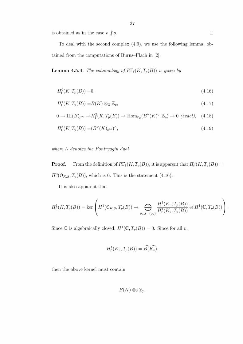
Lemma 4.5.4. The cohomology of RΓf(K,Tp(B)) is given by
H0f (K,Tp(B)) =0, (4.16)
H1f (K,Tp(B)) =B(K)⊗Z Zp, (4.17)
0→ III(B)p∞ →H2f (K,Tp(B))→ HomZp(B
∨(K)c,Zp)→ 0 (exact), (4.18)
H3f (K,Tp(B)) =(B∨(K)p∞)∧, (4.19)
where ∧ denotes the Pontryagin dual.
Proof. From the definition ofRΓf(K,Tp(B)), it is apparent thatH0f (K,Tp(B)) =
H0(OK,S, Tp(B)), which is 0. This is the statement (4.16).
It is also apparent that
H1f (K,Tp(B)) = ker
H1(OK,S, Tp(B))→⊕
v∈S−∞
H1(Kv, Tp(B))
H1f (Kv, Tp(B))
⊕H1(C, Tp(B))
.
Since C is algebraically closed, H1(C, Tp(B)) = 0. Since for all v,
H1f (Kv, Tp(B)) = B(Kv),
then the above kernel must contain
B(K)⊗Z Zp.

38
Since III(B), which is finite, surjects onto the kernel of
H1(OK,S, Vp(B)/Tp(B))
H1f (K,Tp(B))⊗Qp/Zp
→⊕
v∈S−∞
H1(Kv, Vp(B)/Tp(B))
H1f (Kv, Tp(B))⊗Qp/Zp
,
B(K)⊗Z Zp is in fact all of H1f (K,Tp(B)). This is statement (4.17).
To prove the statement (4.18), we use four pairings. The Weil pairing is
Tp(B)× Tp(B∨) // Zp(1) .
Second, we have the Pontryagin pairing
Tp(B)×B∨p∞
// Qp/Zp(1)
Vp(B∨)/Tp(B
∨)
.
Third, we have Poitou-Tate duality
H2c (OK,S, Tp(B))×H1(OK,Sp , Vp(B
∨)/Tp(B∨)(1)) // H3
c (OK,S,Qp/Zp(1))
trace
Qp/Zp.
We obtain
0 // H2f (K,Tp(B))∧ // H1(OK,S, B
∨p∞) //⊕
v∈S−∞H1(Kv ,B∨p∞ )
H1f (Kv ,Tp(B))⊥
.
Then we see that H2f (K,Tp(B))∧ is just the Selmer group Sel(B∨)p∞ , and
H1f (Kv, Tp(B))⊥ = (B(Kv))
⊥, which is B∨(Kv)⊗Qp/Zp. Consider the Galois

39
cohomology exact sequence
0→ B∨(K)⊗Qp/Zp → Sel(B∨p∞)→ III(B∨
p∞)→ 0. (4.20)
We use a fourth pairing, the Cassels–Tate pairing, which says that
III(B∨p∞)∧ ∼ III(B)p∞ .
Also, we know that the Pontryagin dual ofB∨(K)⊗Qp/Zp is HomZp(B∨(K),Zp).
Therefore, dualizing (4.20), we find that
0→ III(B)p∞ → H2f (K,Tp(B))→ HomZp(B
∨(K),Zp)→ 0.
The statement (4.19) follows from Tate–Poitou duality:
H3f (K,Tp(B))
'H3c (OK,S, Tp(B))
'H0(OK,S, V∨p (B)/T∨
p (B)(1))∧
'(B∨(K)p∞)∧
From this lemma we deduce a corollary which identifies the rational coho-
mology.

40
Corollary 4.5.5. The cohomology of RΓf(K,Vp(B)) is given by
H0f (K,Vp(B)) =0, (4.21)
H1f (K,Vp(B)) 'B(K)⊗Z Qp, (4.22)
H2f (K,Vp(B)) '(B∨(K)c ⊗Z Qp)
∨, (4.23)
H3f (K,Vp(B)) =0, (4.24)
where c denotes the conjugate Gal(K/K)-action.
The following lemma describes (4.10), the last of the three complexes.
Lemma 4.5.6. For RΓ(C, Tp(B)) ⊂ RΓ(C, Vp(B)), we have:
detOK,p
H0(C, Tp(B)) =b−1 ·
[F :K]∧j=1
γj
(4.25)
⊂Kp ·
[F :K]∧j=1
γj
= detKp
H0(C, Vp(B)), (4.26)
detOK,p
Hj(C, Tp(B)) =OK,p (4.27)
⊂Kp = detKp
Hj(C, Vp(B)) for j 6= 0. (4.28)
Proof. This result follows from the definition of b.
The last thing we need to translate Gross’ Conjecture is a map relating KΞ
to the determinant of the complex RΓc(OK,S, Vp(B)).
Lemma 4.5.7. There is a K ⊗Q Qp-linear isomorphism induced by the trian-
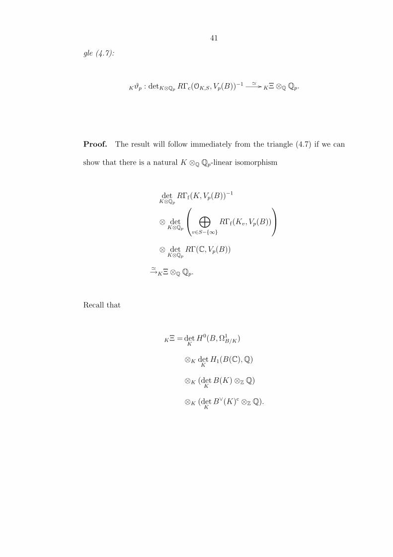
41
gle (4.7):
Kϑp : detK⊗Qp RΓc(OK,S, Vp(B))−1 ' //KΞ⊗Q Qp.
Proof. The result will follow immediately from the triangle (4.7) if we can
show that there is a natural K ⊗Q Qp-linear isomorphism
detK⊗Qp
RΓf(K,Vp(B))−1
⊗ detK⊗Qp
⊕v∈S−∞
RΓf(Kv, Vp(B))
⊗ det
K⊗QpRΓ(C, Vp(B))
'→KΞ⊗Q Qp.
Recall that
KΞ = detKH0(B,Ω1
B/K)
⊗K detKH1(B(C),Q)
⊗K (detKB(K)⊗Z Q)
⊗K (detKB∨(K)c ⊗Z Q).

42
First,
H0(C, Vp(B)) 'H1(B(C),Q)⊗Qp,
Hj(C, Vp(B)) =0 for j 6= 0,
whence
detK⊗Qp
RΓ(C, Vp(B)) = detK⊗Qp
(H1(B(C),Q)⊗Qp).
Second, for v | p,
H1f (Kv, Vp(B))∨
'exp∗
// H0(B,Ω1B/K),
Hjf (Kv, Vp(B) = 0 for j 6= 1,
the isomorphism being given by dual of the exponential map discussed in
Section 4.4, whence
detK⊗Qp
⊕v|p
RΓf(Kv, Vp(B))
' detKH0(B,Ω1
B/K),
while for v 6 | p,
RΓf(Kv, Vp(B)) is acyclic.

43
Third, Lemma 4.5.5 says that
H1f (K,Vp(B)) =B(K)⊗Z Qp,
H2f (K,Vp(B)) =(B∨(K)c ⊗Z Qp)
∨,
Hjf (K,Vp(B)) =0 for j 6= 1, 2,
whence
detK⊗Qp
RΓf(K,Vp(B))−1 =( detK⊗Qp
B(K)⊗Z Qp)
⊗K⊗Qp ( detK⊗Qp
B∨(K)c ⊗Z Qp).
We obtain the K ⊗Q Qp-linear isomophism
detK⊗Qp
RΓf(K,Vp(B))−1
⊗ detK⊗Qp
⊕v∈S−∞
RΓf(Kv, Vp(B))
⊗ det
K⊗QpRΓ(C, Vp(B))
'→KΞ⊗Q Qp
and the result follows.
Now we can reformulate the p-part of Gross’ Conjecture.
Theorem 4.5.8. The p-part of Gross’ Conjecture is equivalent to the state-
ment that
L(ψ, s) ∼ c(s− 1)rankOKB(K) as s→ 1

44
for some constant c ∈ C∗ such that
Kϑ−1∞ (c) ∈ KΞ⊗ 1
and that
OK,p · Kϑ−1p (Kϑ
−1∞ (c)) = det
OK,pRΓc(OK,S, Tp(B))−1.
Proof. Let us examine the isomophism Kϑ∞. From the pairings (4.1) and
(4.2), we find that the image under Kϑ∞ of the generator of KΞ given by the
chosen bases (γjj, ωjj, and xjj), is
Ω · detOK,p
(< xj, xk >)j,k = ΩRC
∣∣∣∣B(K)
X
∣∣∣∣ .So the statements
Kϑ−1∞ (c) ⊂ KΞ⊗ 1
and
OK,p · Kϑ−1p (Kϑ
−1∞ (c)) = det
OK,pRΓc(OK,S, Tp(B))−1
are equivalent to
c
RCΩ∈ K (4.29)
and
OK,p · Kϑ−1∞
(c
RCΩ
)= Kϑp
(detOK,p
RΓc(OK,S, Tp(B))−1
)(4.30)

45
(using for the second equality the fact that B∨(K) ' B(K)).
The first statement of Gross’ Conjecture is just inclusion (4.29), and the
p-part of the second is exactly
(c
RCΩ
)p
=
b · d ·#(III(B)) ·∏v 6 |∞
#
(Bv(kv)
B0v(kv)
)p
, (4.31)
or, equivalently,
OK,p · Kϑ−1∞
(c
RCΩ
)= OK,p · Kϑ−1
∞
b · d ·#(III(B)) ·∏v 6 |∞
#
(Bv(kv)
B0v(kv)
) .
(4.32)
Comparing (4.30) and(4.32), we see from the triangle (4.7) what must be
proven: that
Kϑp
(detOK,p
RΓc(OK,S, Tp(B))−1
)
is generated, in
detKpRΓf(K,Vp(B))−1
⊗ detKp
⊕v∈S−∞
RΓf(Kv, Vp(B)
⊗ det
KpRΓ(C, Vp(B)),
by
b · d ·#(III(B)) ·∏v 6 |∞
#
(Bv(kv)
B0v(kv)
),

46
with respect to the chosen bases.
But this follows from Lemma 4.5.1, Lemma 4.5.4 and its Corollary 4.5.5,
and Lemma 4.5.6.

47
Chapter 5
Elliptic curves with nonmaximalendomorphism ring.
In order to study an elliptic curve E with nonmaximal endomorphism ring,
and its Weil restriction B, we employ another elliptic curve isogenous to E
and defined over the same base field F as E.
Lemma 5.0.1 ([21], Exercise II.1.2). Suppose E is an elliptic curve over
a (number) field F with EndF (E) ' O ⊆ OK. Then there exists an elliptic
curve E0 over F with EndF (E0) ' OK, and an isogeny E → E0 over F .
Proof. Say that OK is generated over Z by 1 and α, and that
O = Z + f · OK = Z + fα · Z.
Define E0 by the following commutative diagram, with exact row and di-

48
agonal:
0 // Ef //
@@@
@@@@
@ E[f ] //
[fα]
E
E
AAA
AAAA
E0
@@@
@@@@
@
0
We shall construct an OK-action on E0 which agrees with the O-action on
E . We construct morphisms υ1, υ2, υ3, as shown in the following diagram:
Ef
AAA
AAAA
A
0 // Ef //
AAA
AAAA
A E //
υ1
E
AAA
AAAA
A
υ2
E
BBB
BBBB
B E0
???
????
?
υ3~~E0
!!BBB
BBBB
B 0
0
The upper diagonal is the same as the lower diagonal. The morphism υ1 is
defined by commutativity. The morphism υ2 is obtained by observing that the
kernel of the morphism
E[f ] // E
is contained in the kernel of υ1. The morphism υ3 is obtained as follows. The

49
kernel of the upper diagonal morphism
E
AAA
AAAA
E0
is the image of the composite morphism:
Ef // E
[fα]
E
This image is
[fα]Ef ,
which has pre-image
[fα]Ef2
under
E[f ] // E ,
whose image under
E
[fα]
E

50
is
[fα]2Ef2
=[f 2α2]Ef2
=[fα2]Ef
=[f(aα+ b)]Ef2 for some a, b ∈ Z
=([a][fα] + [b][f ])Ef
=[a][fα]Ef ,
which is contained in the kernel of the lower diagonal morphism:
E
AAA
AAAA
E0
Therefore, the kernel of the upper diagonal morphism
E
AAA
AAAA
E0
(in which we were originally interested) is contained in the kernel of υ2, and
υ3 can be constructed making the diagram commute. We then define
[α] : E0 → E0

51
to be υ3. The morphisms
1 = id : E0 → E0
and
[α] : E0 → E0
are extended by linearity to an action of OK upon E0.
One checks that this action is a well-defined ring action and agrees with
the action of O upon E. That is, for any x ∈ O ⊂ OK , the diagram
E[x] //
E
E0
[x] // E0
commutes.
It is known (see for example [20], Appendix C, Theorem 11.5) that the
j-invariant of E (resp. E0) belongs to the ring class field H(O) associated to
O (resp .the Hilbert class field H = H(OK) of K). We have a tower of fields
K ⊂ H ⊂ H(O) ⊂ F . The curves E and E0 are twists over F of elliptic curves
defined over H(O) and H, respectively.
As before, we have B the Weil restriction of E, and we define B0 to be the
Weil restriction of E0. The varieties B and B0 are isogenous abelian varieties
over K with complex multiplication by O and OK , respectively.

52
5.1 The Burns–Flach Conjecture.
The elliptic curve E is defined over F , with complex multiplication by the
order O ⊆ OK , with Weil restriction B := ResFKE, and with E having
Grossencharacter ψ. The Burns–Flach Conjecture concerns the Weil restric-
tion B of the original elliptic curve E.
Let f be the conductor of F . Fix a prime p. Let S, a set of places of K, be
defined as the union of the set of prime divisors of fp, and the set of primes
below those of bad reduction of E/F , along with the infinite place. Then by
the Criterion of Neron–Ogg–Safarevic, S −∞ is the set of places where the
extensions F (Epn)/K are ramified.
Conjecture 5.1.1 (Burns–Flach). We have
L(ψ, s) ∼ c(s− 1)rankOKB(K) as s→ 1
for some constant c ∈ C∗ such that
Kϑ−1∞ (c) ∈ KΞ⊗ 1
and
Op · Kϑ−1p (Kϑ
−1∞ (c)) = det
OpRΓc(OK,S, Tp(B))−1. (5.1)
Note 5.1.2. The Burns–Flach Conjecture is a strengthening of the p-part of
Gross’ Conjecture (for primes p dividing the conductor of O). Taking tensor

53
products with OK,p in the statement of the Burns–Flach Conjecture, we have
Tp(B)⊗Op OK,p = Tp(B0), and the determinant over Op becomes a determinant
over OK,p, yielding the p-part of the statement of Gross’ Conjecture.
5.2 A refinement in the case F (Etors)/K is abelian.
We wish to refine the conjecture further by considering the full endomorphism
algebra of B, which can be much larger than K. Write R := EndK(B),
R := R⊗Z Q, Rp := R⊗Z Zp, and Rp := R⊗Z Qp = R⊗Q Qp.
Lemma 5.2.1. Suppose F (Etors)/K is abelian. Then R is a commutative
semisimple K-algebra of rank [F : K]. Also, R is projective over O and Tp(B)
is projective over Rp.
Proof. R is computed in [8] Section 4. R = EndK(B) is the Galois invariants
of EndF (B), where B is isomorphic over F to
∏σ∈G
Eσ.
Therefore R is the Galois invariants of
HomF
(∏σ∈G
Eσ,∏σ∈G
Eσ
)=
∏σ1,σ2∈G
Hom(Eσ1 , Eσ2),
which is seen to be ∏σ∈G
Hom(Eσ, E) · σ.
Thus R is projective over O. As well, as in [8], §4, R is a commutative semisim-
54
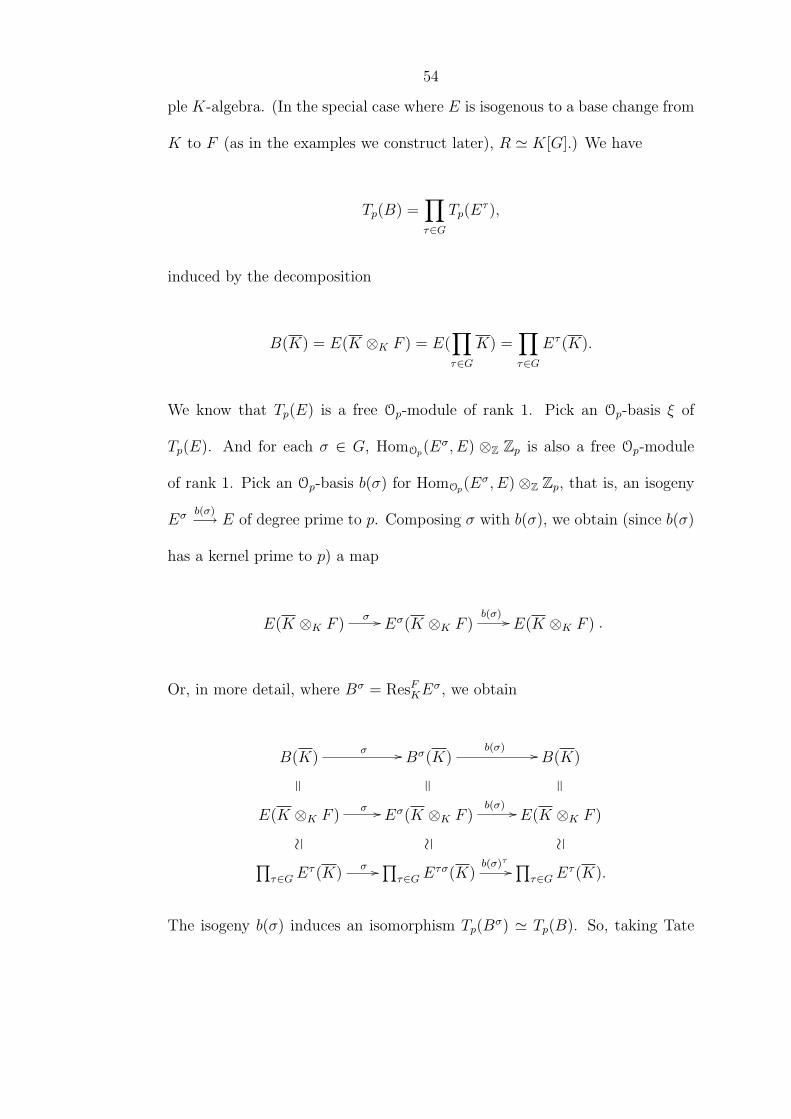
ple K-algebra. (In the special case where E is isogenous to a base change from
K to F (as in the examples we construct later), R ' K[G].) We have
Tp(B) =∏τ∈G
Tp(Eτ ),
induced by the decomposition
B(K) = E(K ⊗K F ) = E(∏τ∈G
K) =∏τ∈G
Eτ (K).
We know that Tp(E) is a free Op-module of rank 1. Pick an Op-basis ξ of
Tp(E). And for each σ ∈ G, HomOp(Eσ, E) ⊗Z Zp is also a free Op-module
of rank 1. Pick an Op-basis b(σ) for HomOp(Eσ, E)⊗Z Zp, that is, an isogeny
Eσ b(σ)−→ E of degree prime to p. Composing σ with b(σ), we obtain (since b(σ)
has a kernel prime to p) a map
E(K ⊗K F )σ // Eσ(K ⊗K F )
b(σ) // E(K ⊗K F ) .
Or, in more detail, where Bσ = ResFKEσ, we obtain
B(K)σ // Bσ(K)
b(σ) // B(K)
E(K ⊗K F )σ //
=
Eσ(K ⊗K F )b(σ) //
=
E(K ⊗K F )
=
∏τ∈GE
τ (K)σ //
' ∏τ∈GE
τσ(K)b(σ)τ //
' ∏τ∈GE
τ (K).
'
The isogeny b(σ) induces an isomorphism Tp(Bσ) ' Tp(B). So, taking Tate

55
modules, we obtain the diagram
Tp(B) σ // Tp(Bσ)
b(σ) // Tp(B)
∏τ∈G Tp(E
τ ) σ //= ∏
τ∈G Tp(Eτσ)
b(σ) //
= ∏τ∈G Tp(E
τ )
=
( ξτ=1
, 0, . . . , 0) //
∈
(0, . . . , 0, ξτ=σ−1
, 0, . . . , 0) //
∈
(0, . . . , 0, b(σ)σ−1
τ=σ−1
ξ, 0, . . . , 0)
∈
Since ξ is an Op-basis of Tp(E), then b(σ)σ−1ξ is also an Op-basis of Tp(E).
Suppose
(ατ · b(τ)τ−1
ξ)τ∈G
is any element of ∏τ∈G
Tp(Eτ ) = Tp(B).
We can write
(ατ · b(τ)τ−1
ξ)τ∈G =
(∑τ∈G
ατ · b(τ) · τ
)( ξτ=1
, 0, . . . , 0)
with unique ατ ∈ Op, that is, with unique
(∑τ∈G
ατ · b(τ) · τ
)∈ Rp.
Therefore ( ξτ=1
, 0, . . . , 0) is an Rp-basis of Tp(B). In particular, Tp(B) is a
projective Rp-module.

56
We define an L-function for B as we did for E,
RL(B/K, s) :=∏w 6 |∞
RPw(B/K,Nw−s)−1 : C→ R⊗Q C,
where
RPw(B/K, x) = detR⊗Q`
(1− xφw | (T`(B)⊗Q`)Iw).
Write ϕ for a Grossencharacter of K, which when pre-composed with the
norm, gives ψ. Then, as in [8], the possible choices for ϕ are ϕχ : χ ∈ G.
Writing X for the set of orbits of ϕχ : χ ∈ G under AutKC, we have
R = K ⊗O R = K ⊗O EndKB '∏X
K(ϕχ),
where K(ϕχ) is K with the values of ϕχ adjoined. The L-function RL(B, s)
corresponds to the tuple of functions
(L(σ(ϕχ), s))X,σ∈HomK(K(ϕχ),C),
which is considered an element of R⊗Q C, where
R '∏X
K(ϕχ).
57
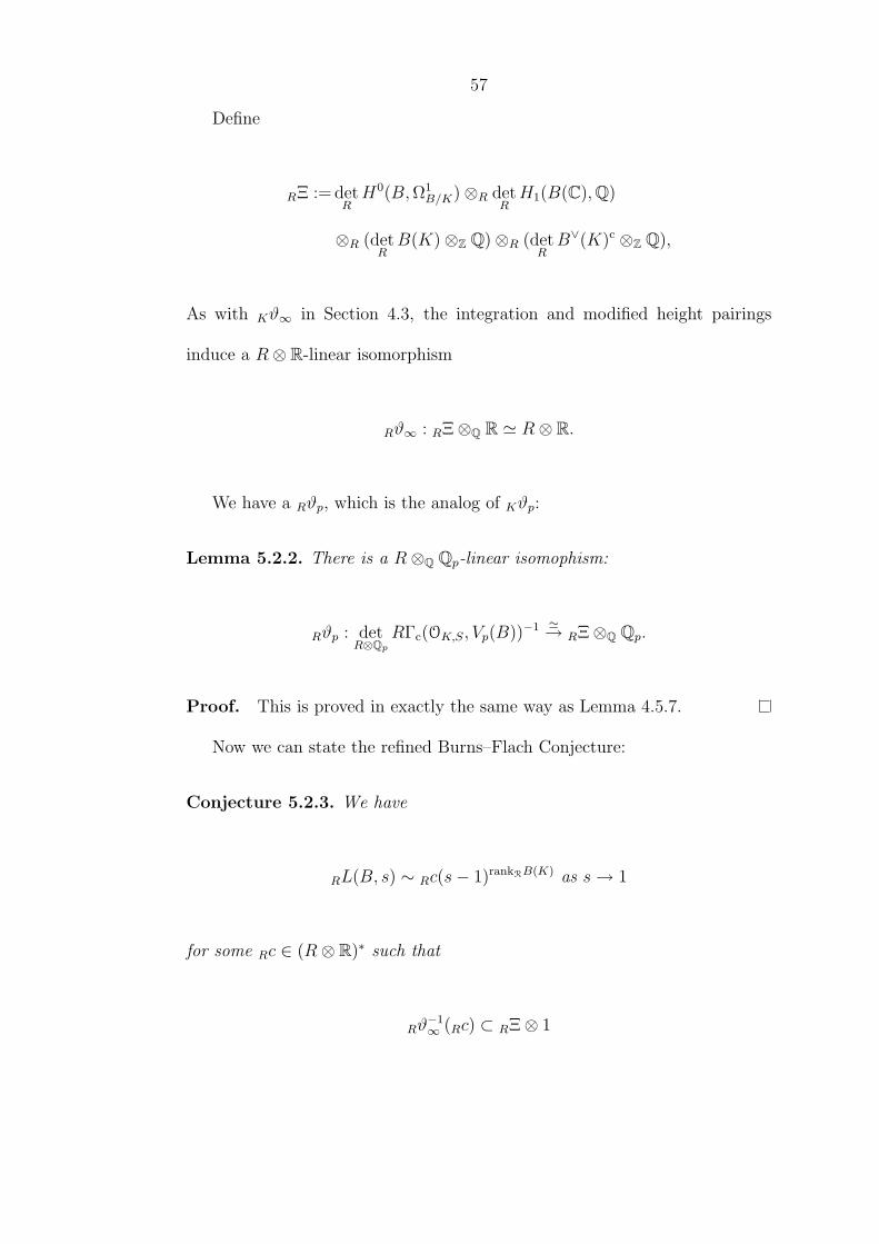
Define
RΞ := detRH0(B,Ω1
B/K)⊗R detRH1(B(C),Q)
⊗R (detRB(K)⊗Z Q)⊗R (det
RB∨(K)c ⊗Z Q),
As with Kϑ∞ in Section 4.3, the integration and modified height pairings
induce a R⊗ R-linear isomorphism
Rϑ∞ : RΞ⊗Q R ' R⊗ R.
We have a Rϑp, which is the analog of Kϑp:
Lemma 5.2.2. There is a R⊗Q Qp-linear isomophism:
Rϑp : detR⊗Qp
RΓc(OK,S, Vp(B))−1 '→ RΞ⊗Q Qp.
Proof. This is proved in exactly the same way as Lemma 4.5.7.
Now we can state the refined Burns–Flach Conjecture:
Conjecture 5.2.3. We have
RL(B, s) ∼ Rc(s− 1)rankRB(K) as s→ 1
for some Rc ∈ (R⊗ R)∗ such that
Rϑ−1∞ (Rc) ⊂ RΞ⊗ 1
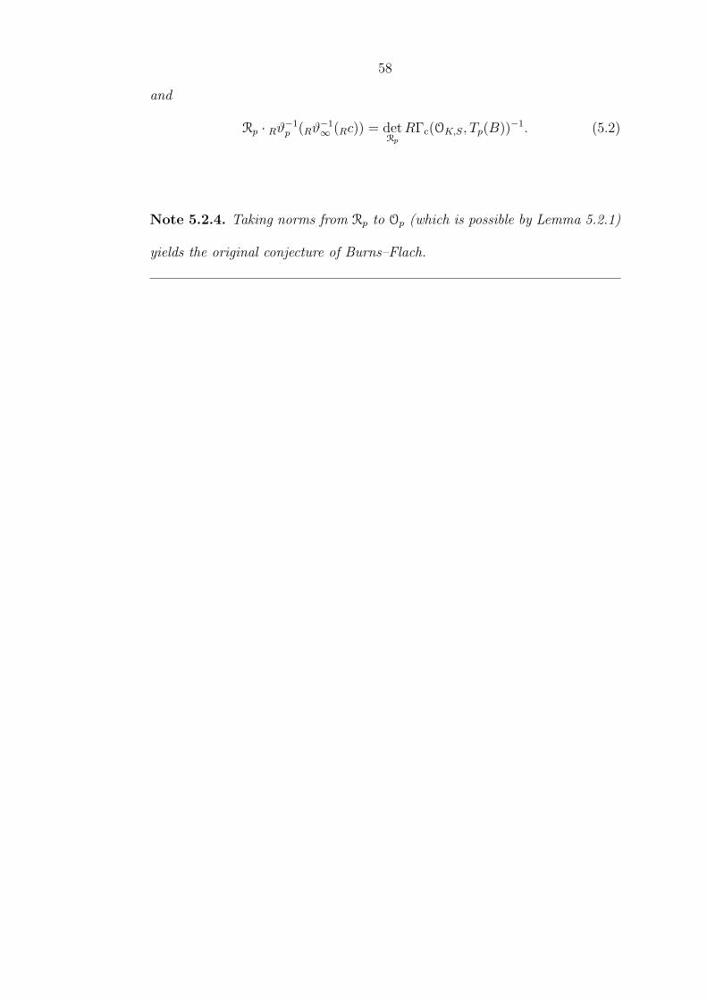
58
and
Rp · Rϑ−1p (Rϑ
−1∞ (Rc)) = det
RpRΓc(OK,S, Tp(B))−1. (5.2)
Note 5.2.4. Taking norms from Rp to Op (which is possible by Lemma 5.2.1)
yields the original conjecture of Burns–Flach.
59
Chapter 6
Translation into theterminology of Kato.
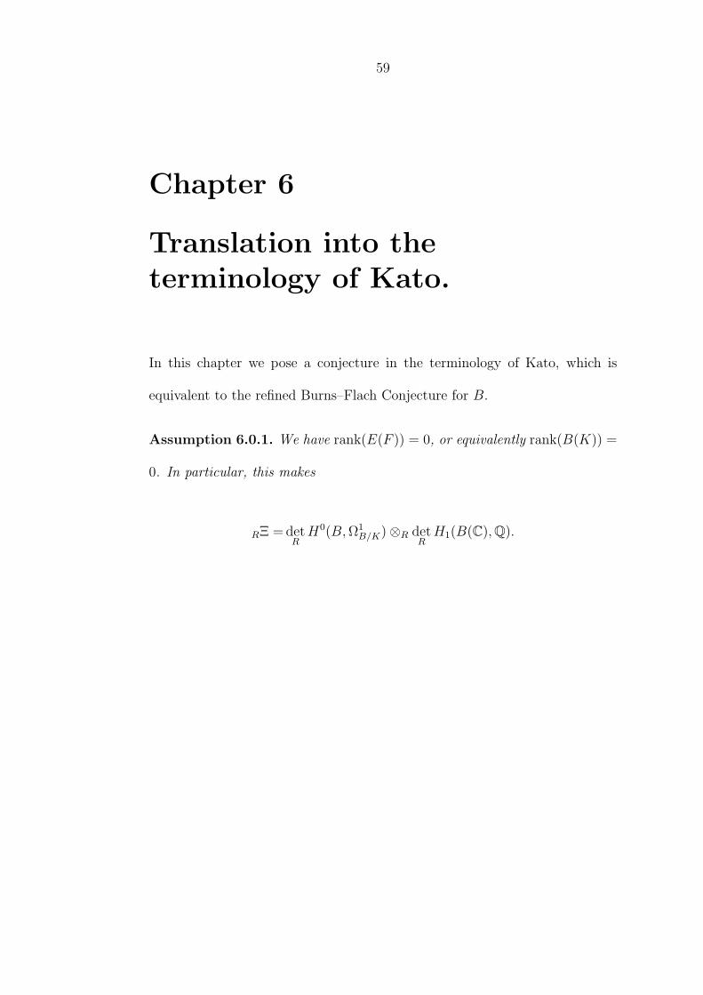
In this chapter we pose a conjecture in the terminology of Kato, which is
equivalent to the refined Burns–Flach Conjecture for B.
Assumption 6.0.1. We have rank(E(F )) = 0, or equivalently rank(B(K)) =
0. In particular, this makes
RΞ = detRH0(B,Ω1
B/K)⊗R detRH1(B(C),Q).

60
For ease of notation, we will now write the following:
T :=Tp(B)
V :=Vp(B)
Ξ :=RΞ
ϑ∞ :=Rϑ∞
ϑp :=Rϑp
c :=Rc
The Rp-sheaf T on SpecOK,S is smooth and invertible. Define the invertible
Rp-module
∆Rp(OK,S, T )
to be
(detRp
(RΓ(OK,S, T ))
)−1
⊗Rp
(detRp
(RΓ(OK,S ⊗Z R, T (−1)))
)−1
,
and
∆Rp(OK,S, V )
to be
∆Rp(OK,S, T )⊗Zp Qp
We compute the cohomology of RΓ(OK,S, V ) as follows:
Lemma 6.0.2. • H1(OK,S, V ) is a 1-dimensional Rp-vector space.

61
• Hj(OK,S, V ) = 0 for j 6= 1.
Proof. Use the exact triangle
RfΓ(OK,S, V )→ RΓ(OK,S, V )→⊕v∈S
R/fΓ(Kv, V )
(see [4], §3.2), which is the complex
0→H0f (K,V )→ H0(OK,S, V )→
⊕v∈S
H0/f(Kv, V )
→H1f (K,V )→ H1(OK,S, V )→
⊕v∈S
H1/f(Kv, V )
→H2f (K,V )→ H2(OK,S, V )→
⊕v∈S
H2/f(Kv, V )
→H3f (K,V )→ · · · .
Now H0(OK,S, V ) = 0, and since RΓf(K,V ) is acyclic by Assumption 6.0.1,
we have
H1(OK,S, V ) '⊕v∈S
H1/f(Kv, V ),
H2(OK,S, V ) '⊕v∈S
H2/f(Kv, V ),

62
the second giving us by duality
H2(OK,S, V ) '⊕v∈S
H2/f(Kv, V )
'⊕v∈S
H2(Kv, V )
'⊕v∈S
H0(Kv, V∗(1))∗
'⊕v∈S
H0(Kv, V )∗
since V is the Weil restriction of an elliptic curve
=0.
Consider the exact sequence
0 // H1f (Kv, V ) // H1(Kv, V ) // H1
/f(Kv, V ) // 0
0
.
If v 6 | p, then H1(Kv, V ) = 0, and for v | p, we compute
dimRp H1(OK,S, V ) =
∑v|p
dimRp H1/f(Kv, V )
=∑v|p
dimRp H1(Kv, V ).

63
Using Kp =∏
v|pKv we rewrite this:
dimOp Rp · dimRp H1(OK,S, V ) = dimOp Rp ·
∑v|p
dimRp H1(Kp, V )
=∑v|p
dimOp H1(Kp, V )
Applying Tate’s Euler characteristic formula
dimOp H0(Kv, V )− dimOp H
1(Kv, V ) + dimOp H2(Kv, V )
=− [Kv : Qp] dimOp ,
with
H0(Kv, V ) = H2(Kv, V ) = 0,
we obtain
dimOp Rp · dimRp H1(OK,S, V ) =[Kp : Qp] dimOp V
=[Kp : Qp] dimOp Rp,
where the last equality follows from
dimRp V = 1.

64
Further, we find
dimOp Rp · dimRp H1(OK,S, V ) =[Kp : Qp] dimOp Rp,
=[Kp : Qp] dimOp B
= dimOp B(Kp)⊗Zp Qp,
⇒ dimRp H1(OK,S, V ) = dimRp B(Kp)⊗Zp Qp,
so that
H1(OK,S, V )
has dimension 1 over Rp.
The dual exponential map (see [13] Chapter II §1.2-§1.4) is
exp∗ : H1(K,V )→ H0(B,Ω1B/K),
and gives us a map
detRp
(exp∗ ⊗ id) : ∆Rp(OK,S, V )→ Ξ⊗Qp,
the determinant of Kato’s exp∗ ⊗ id.
Note that for v ∈ S − ∞, all terms in RΓf(Kv, V ) are zero except for
possiblyH1f (Kv, V ), and that all terms in RΓ(C, V ) are zero except for possibly
H0(C, V ).
The modules involved in the refined Burns–Flach Conjecture are in fact
isomorphic to those just defined above. We summarize the situation in the

65
following two lemmata.
Lemma 6.0.3.
detRp
RΓc(OK,S, T )−1 ' ∆Rp(OK,S, T )
Proof. We use the complex RΓc(OK,S, T ) which is defined in this case by
the exact triangle
RΓc(OK,S, T )→ RΓ(OK,S, T )→⊕
v∈S−∞
RΓ(Kv, T ).
We consider the following exact triangle which it satisfies:
RΓc(OK,S, T ) // RΓc(OK,S, T ) // RΓ(C, T ) (6.1)
Tate–Poitou duality gives
detRp
RΓc(OK,S, T ) ' detRp
RΓ(OK,S, T∗(1))∗[−3]
66
So from (6.1),
detRp
RΓc(OK,S, T (1)) ' detRp
RΓc(OK,S, T )⊗Rp detRp
RΓ(OK,S ⊗ R, T )−1
' detRp
RΓc(OK,S, T∗(1))∗[−3]⊗Rp det
RpRΓ(OK,S ⊗ R, T )−1
'−1
detRp
RΓc(OK,S, T∗(1))∗ ⊗Rp det
RpRΓ(OK,S ⊗ R, T )−1
' detRp
RΓc(OK,S, T∗(1))# ⊗Rp det
RpRΓ(OK,S ⊗ R, T (−1))
since T ∗(1) ' T#, whence T ∗# ' T (−1),
' detRp
RΓc(OK,S, T )⊗Rp detRp
RΓ(OK,S ⊗ R, T (−1))
where “∗” denotes RHom(•,Zp) and “#” means changing the Rp-action via
the (Rosati) involution on Rp. We conclude that
detRp
RΓc(OK,S, T )−1
=
(detRp
(RΓ(OK,S, T ))
)−1
⊗Rp
(detRp
(RΓ(OK,S ⊗ R, T (−1)))
)−1
is isomorphic to
∆Rp(OK,S, T ).
This proves Lemma 6.0.3.
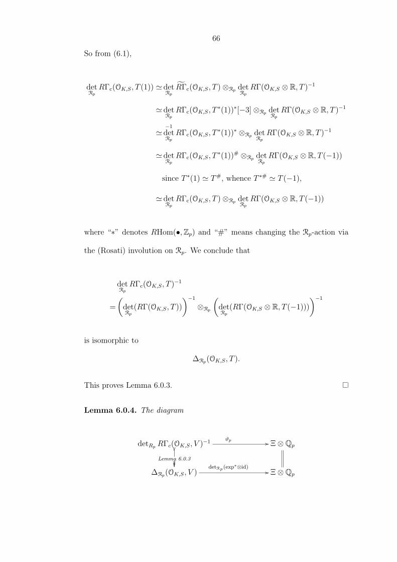
Lemma 6.0.4. The diagram
detRp RΓc(OK,S, V )−1 ϑp //
Lemma 6.0.3
Ξ⊗Qp
∆Rp(OK,S, V )detRp (exp∗⊗id)
// Ξ⊗Qp

67
commutes, where
detRp
(exp∗ ⊗ id)
the determinant of Kato’s exp∗ ⊗ id.
Proof. The map ϑp is constructed from the dual exponential maps
H1f (Kv, Vp(B))∨
'exp∗
// H0(B,Ω1B/K),
for v | p. The left vertical arrow is obtained from dualities and defining
exact triangles, so that the composition of the left vertical map and the lower
horizontal map detRp(exp∗ ⊗ id) is another exponential map, which at v | p is
exp∗.
Knowing that the last two results are true, we can now pose the refined
Burns–Flach Conjecture in the terminology of Kato.
Conjecture 6.0.5. We have
ϑ−1∞ (RL(B, 1)) ⊂ Ξ⊗ 1 (6.2)
and
Rp · det(exp∗⊗id)−1(ϑ−1∞ (RL(B, 1)) = ∆Rp(OK,S, T ). (6.3)

68
Chapter 7
Proof of the conjecture.
The proof will be indicated in this chapter, with more details being given in
the following chapters.
7.1 A universal situation.
Following Kato, we now pass to a situation universal with respect to invertible
sheaves over p-adic rings such as Tp(B) over Rp.
Write Km for the ray class field modulo m, and let f be the conductor of
B. Recall that S is the set of places of K dividing ∞fp. Put
Λn :=Zp[Gal(K fpn/K)],
Λ∞ :=lim←−n
Λn = Zp[Gal(K fp∞/K)] (the completed Galois group algebra),
Fn :=(fKfpn )∗(fKfpn )∗(Zp(1)SpecOK,S)
(fL being the canonical morphism SpecOL,S → SpecOK,S),
F∞ :=lim←−n
Fn
69
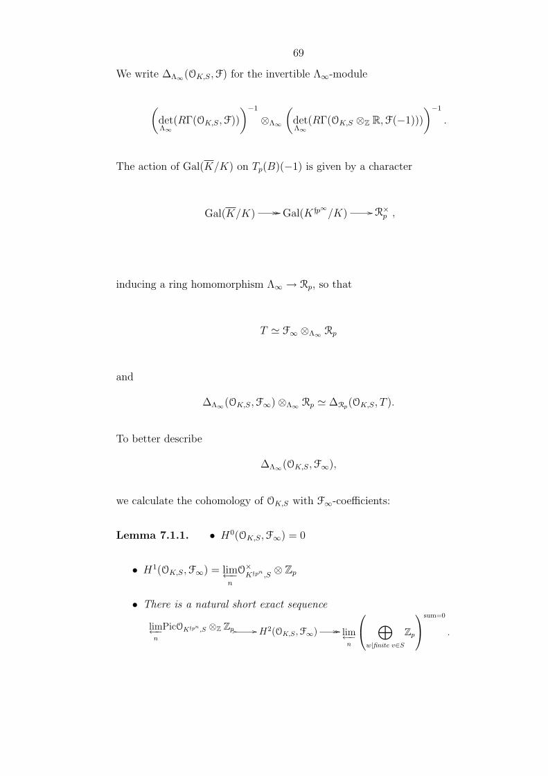
We write ∆Λ∞(OK,S,F) for the invertible Λ∞-module
(detΛ∞
(RΓ(OK,S,F))
)−1
⊗Λ∞
(detΛ∞
(RΓ(OK,S ⊗Z R,F(−1)))
)−1
.
The action of Gal(K/K) on Tp(B)(−1) is given by a character
Gal(K/K) // // Gal(K fp∞/K) // R×p ,
inducing a ring homomorphism Λ∞ → Rp, so that
T ' F∞ ⊗Λ∞ Rp
and
∆Λ∞(OK,S,F∞)⊗Λ∞ Rp ' ∆Rp(OK,S, T ).
To better describe
∆Λ∞(OK,S,F∞),
we calculate the cohomology of OK,S with F∞-coefficients:
Lemma 7.1.1. • H0(OK,S,F∞) = 0
• H1(OK,S,F∞) = lim←−n
O×Kfpn ,S
⊗ Zp
• There is a natural short exact sequence
lim←−n
PicOKfpn ,S ⊗Z Zp // // H2(OK,S,F∞) // // lim←−n
⊕w|finite v∈S
Zp
sum=0
.

70
Proof. We use the short exact sequence
0 // µpk // Gmpk // Gm
// 0 ,
for which the Kummer sequence yields the following exact sequences:
0 // H0(OKfpn ,S, µpk) // // H0(OKfpn ,S,Gm)pk
H0(OKfpn ,S,Gm)/pk // // H1(OKfpn ,S, µpk) // // H1(OKfpn ,S,Gm)pk
H1(OKfpn ,S,Gm)/pk // H2(OKfpn ,S, µpk) // H2(OKfpn ,S,Gm)pk
BrS(OKfpn )pk
Take projective limits lim←−k
to obtain the following exact sequences:
0 // H0(OKfpn ,S,Zp(1)) // 0
OKfpn ,S ⊗Z Zp, // // H1(OKfpn ,S,Zp(1)) // // 0
PicOKfpn ,S ⊗Z Zp// // H2(OKfpn ,S,Zp(1)) // //
⊕w|finite v∈S
Zp
sum=0
Take projective limits again, this time lim←−n
, we find
H0(OK,S,F∞) = 0

71
and
lim←−n
OKfpn ,S ⊗Z Zp = H1(OK,S,F∞),
and obtain another exact sequence:
lim←−n
PicOKfpn ,S ⊗Z Zp // // H2(OK,S,F∞) // // lim←−n
⊕w|finite v∈S
Zp
sum=0
Thus the result is proved.
We now use a construction of Kato ([13], III, §1.2). We will use his
Assumption 7.1.2. K has class number 1.
Kato’s E, and its Grossencharacter ν, we will denote by E0 and ϕ, respec-
tively. Now, our E0/K is an elliptic curve isogenous to our E of Chapter 5
and Chapter 6, and with complex multiplication by the full ring of integers
OK . Then our “ϕ” here is consistent with that of those chapters.
We use the following proposition of Kato (written using our notation).
Proposition 7.1.3 ([13], III, 1.1.5). Suppose a ∈ End(Eχ0 ), (a, 6) = 1.
Then there exists a unique rational function θa ∈ K(Eχ0 )× satisfying the fol-
lowing two conditions:
Nb(θa) = θa for any b ∈ End(Eχ0 ) such that (a, b) = 1. (7.1)
The divisor of θa is deg(a)(e)− ker(a). (7.2)
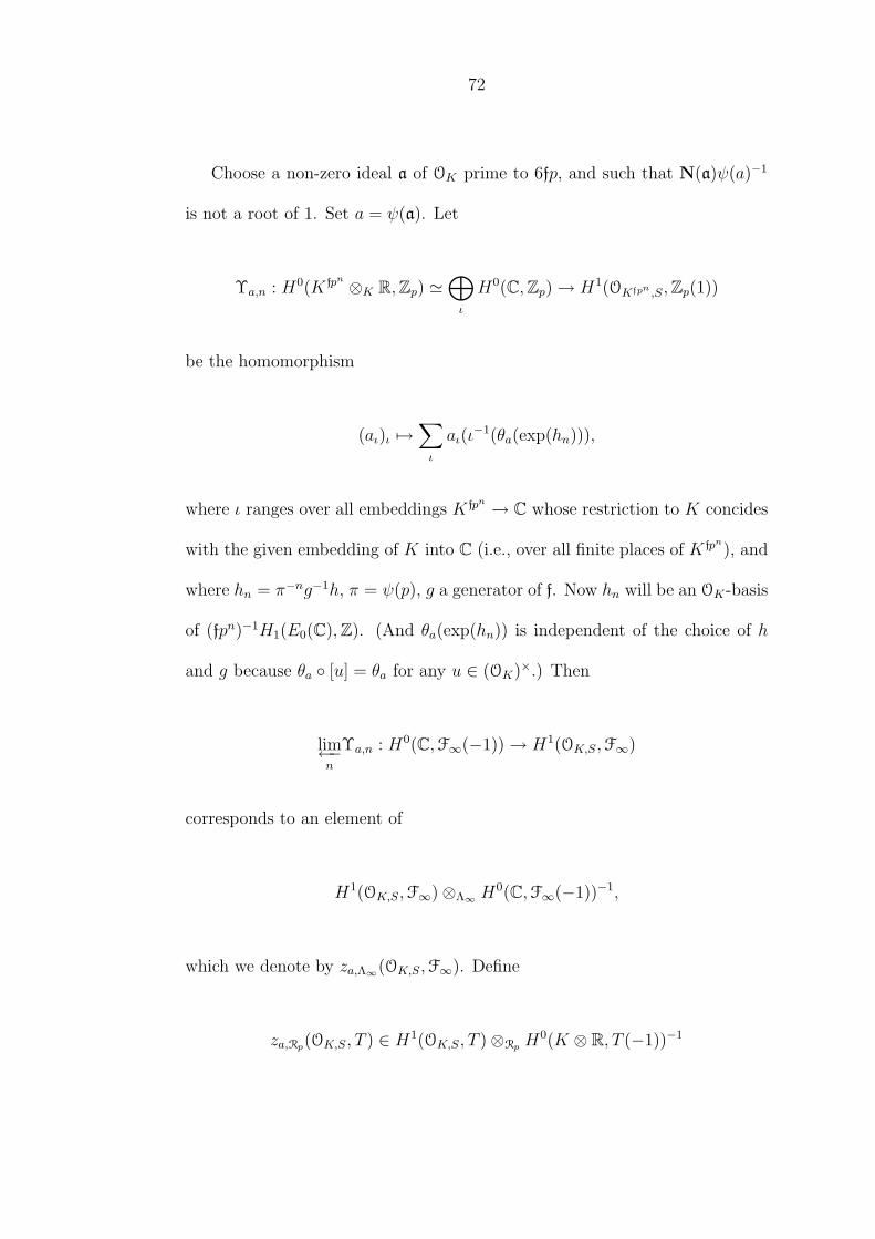
72
Choose a non-zero ideal a of OK prime to 6fp, and such that N(a)ψ(a)−1
is not a root of 1. Set a = ψ(a). Let
Υa,n : H0(K fpn ⊗K R,Zp) '⊕ι
H0(C,Zp)→ H1(OKfpn ,S,Zp(1))
be the homomorphism
(aι)ι 7→∑ι
aι(ι−1(θa(exp(hn))),
where ι ranges over all embeddings K fpn → C whose restriction to K concides
with the given embedding of K into C (i.e., over all finite places of K fpn), and
where hn = π−ng−1h, π = ψ(p), g a generator of f. Now hn will be an OK-basis
of (fpn)−1H1(E0(C),Z). (And θa(exp(hn)) is independent of the choice of h
and g because θa [u] = θa for any u ∈ (OK)×.) Then
lim←−n
Υa,n : H0(C,F∞(−1))→ H1(OK,S,F∞)
corresponds to an element of
H1(OK,S,F∞)⊗Λ∞ H0(C,F∞(−1))−1,
which we denote by za,Λ∞(OK,S,F∞). Define
za,Rp(OK,S, T ) ∈ H1(OK,S, T )⊗Rp H0(K ⊗ R, T (−1))−1
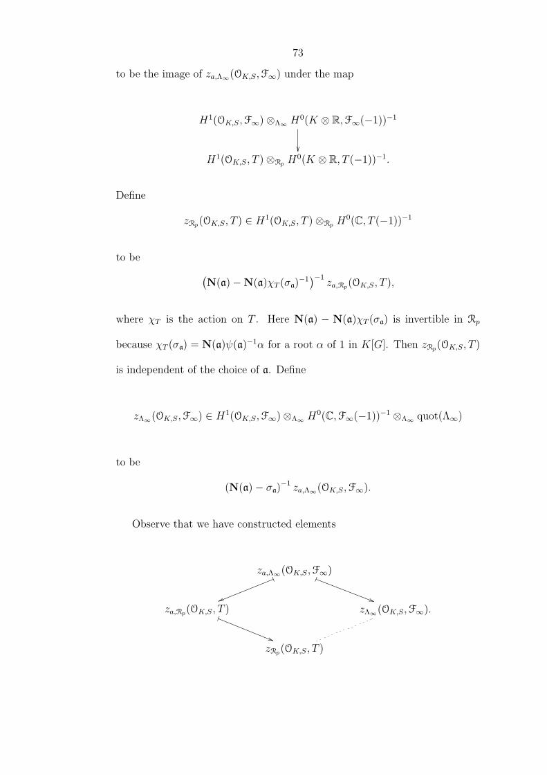
73
to be the image of za,Λ∞(OK,S,F∞) under the map
H1(OK,S,F∞)⊗Λ∞ H0(K ⊗ R,F∞(−1))−1
H1(OK,S, T )⊗Rp H
0(K ⊗ R, T (−1))−1.
Define
zRp(OK,S, T ) ∈ H1(OK,S, T )⊗Rp H0(C, T (−1))−1
to be (N(a)−N(a)χT (σa)
−1)−1
za,Rp(OK,S, T ),
where χT is the action on T . Here N(a) − N(a)χT (σa) is invertible in Rp
because χT (σa) = N(a)ψ(a)−1α for a root α of 1 in K[G]. Then zRp(OK,S, T )
is independent of the choice of a. Define
zΛ∞(OK,S,F∞) ∈ H1(OK,S,F∞)⊗Λ∞ H0(C,F∞(−1))−1 ⊗Λ∞ quot(Λ∞)
to be
(N(a)− σa)−1 za,Λ∞(OK,S,F∞).
Observe that we have constructed elements
za,Λ∞(OK,S,F∞)
))SSSSSSSSSSSSSS,
uulllllllllllll
za,Rp(OK,S, T )
))RRRRRRRRRRRRRzΛ∞(OK,S,F∞).
zRp(OK,S, T )
74
7.2 The strategy of proof.
The rest of our exposition has two parts. First, following the approach of
Kato, we show in §8 that zΛ∞(OK,S,F∞) is an Λ∞-basis of ∆Λ∞(OK,S,F∞),
which allows us to conclude that zRp(OK,S, T ) is a Rp-basis of ∆Rp(OK,S, T ).
Second, we find (Theorem 9.0.2), using [13], III, Theorem 1.2.6, that the image
of zRp(OK,S, T ) under the map
detRp
(exp∗ ⊗ id) : detRp
∆Rp(OK,S, V )→ Ξ⊗Qp
is sent by ϑ∞ to (LS((ϕχ)−1, 0))χ∈G, where LS((ϕχ)−1, 0) equals the L-value
L(ϕχ, 1), deprived of the Euler factors at primes dividing f. But the Euler
factors at primes of bad reduction are 1, and we shall assume that the Euler
factors at any other primes dividing f, are also units at p. So we may disregard
the missing Euler factors.
Our result on the image of
zRp(OK,S, T )
shows that the image of
detRp
∆Rp(OK,S, T )
under exp∗ is generated by (ϑ∞)−1(RL(B/K, 1)), as asserted by the Burns–
Flach Conjecture.
We summarize the strategy of proof, including the translation of the re-

75
fined Burns–Flach Conjecture into the terminology of Kato, in the following
diagram:
detRp RΓc(OK,S, V )−1 'ϑp
//
Lemma 6.0.3
Ξ⊗Qp'ϑ∞
// R⊗ R
∆Rp(OK,S, V ) 'detRp (exp∗⊗id)
// Ξ⊗Qp'ϑ∞
// R⊗ R
∆Rp(OK,S, T )
⊂
zRp(OK,S, T )
∈
//∑
[χ] L(ϕχ, 1)c+[χ]
∈
// (L(ϕχ, 1))[χ]
∈
The first line depicts the morphisms involved in the refined Burns–Flach Con-
jecture. The second line shows the translation into the terminology of Kato.
On the third line is given the integral submodule of the vector space just above.
On the fourth line is a basis for the integral submodule (on the left), and its
images under the two maps of the second line. The element c+[χ] is defined to
be the pre-image, under ϑ∞, of the element of R with [χ]-component 1 and all
other components 0.

76
Chapter 8
A Λ∞-basis of ∆Λ∞(OK,S,F∞).
We will make an
Assumption 8.0.1. • K has class number 1.
• p 6 | [K(f0p) : K], where f0 | f is the prime-to-p part of f.
• p 6 | µ(HK), where HK is the Hilbert Class Field of K.
In this chapter we prove the following
Theorem 8.0.2. Recall that the finite places of S are exactly those dividing
fp. Then
zΛ∞(OK,S,F∞)
is an Λ∞-basis of
∆Λ∞(OK,S,F∞).
To work more easily with the element
zΛ∞(OK,S,F∞) ∈ H1(OK,S,F∞)⊗Rp H0(K ⊗ R,F∞(−1))−1,

77
we fix a basis
yΛ∞(OK,S,F∞)
of
H0(K ⊗ R,F∞(−1))−1.
Here yΛ∞(OK,S,F∞) is an inverse system of embeddings
K fpn → C
which could come, for example, from a fixed embedding Q → C. Now also fix
xa,Λ∞(OK,S,F∞) ∈ H1(OK,S,F∞)
such that
za,Λ∞(OK,S,F∞) = xa,Λ∞(OK,S,F∞)⊗Rp yΛ∞(OK,S,F∞)
and
yΛ∞(OK,S,F∞)
is a basis of H0(K ⊗ R,F∞(−1))−1. Correspondingly, we express
zΛ∞(OK,S,F∞) = xΛ∞(OK,S,F∞)⊗Rp yΛ∞(OK,S,F∞),
where
xΛ∞(OK,S,F∞) = (N(a)− σa)−1xa,Λ∞(OK,S,F∞).

78
The primary result we will be using is the
Theorem 8.0.3 ([17], Theorem 4.1: Main Conjecture).
char(A∞) = char(U∞/C∞),
where
A∞ =lim←−n
An
U∞ =lim←−n
Un
C∞ =lim←−n
Cn,
where An is the p-part of the ideal class group of K fpn, Un is the global units,
and Cn is the elliptic units. The inverse limits are all with respect to the norm
maps.
We need a lemma to permit us to deal with modules over discrete valuation
ring, instead of with the Λ∞-modules themselves.
Lemma 8.0.4. Let N be a local Noetherian integral domain and suppose
I, J ⊂ M are two invertible N-submodules of an invertible quotN-submodule
M . (Since N and quotN are local, “invertible” means free of rank 1.) If N is
Cohen-Macaulay then I = J if and only if Iq = Jq for all height-1 prime ideals
q of N .

79
Proof. The result would follow if we could show that
I =⋂
htq=1
Iq ⊂M and J =⋂
htq=1
Jq ⊂M.
Since Iq = Nq ⊗N I and Jq = Nq ⊗N J , then this would in turn be implied by
N =⋂
htq=1
Nq ⊂ quotN.
The inclusion
N ⊆⋂
htq=1
Nq
is obvious. To prove
N ⊇⋂
htq=1
Nq,
let
quotN 3 xy6∈ N,
where x, y ∈ N . Then y 6∈ N∗,⇒ (y) 6= N , so that y is a (1-term) N -regular
sequence. By [15] §15 Lemma 4, we find that
dimN/(y) = dimN − 1.
But [15] §16 Theorem 31(i) implies that
dimN/(y) = dimN − ht(y).
We conclude that ht(y)=1, which means that y lies in some height-1 prime

80
ideal q of N . Therefore xy6∈ Nq and in particular
x
y6∈⋂
htq=1
Nq.
Note 8.0.5. The ring Λ∞ is
Zp[Gal(K f0p/K)][[Gal(K f0p∞/K f0p)]] ' Zp[Gal(K f0p/K)][[x, y]],
where f0 is the prime-to-p part of f. If p 6 | [K f0p : K] then Zp[Gal(K f0p/K)]
is a product of discrete valuation rings; hence Λ∞ is regular. If p | [K f0p : K]
then Λ∞ is no longer regular. But the ring Λ∞ is a complete intersection and
in particular is Cohen–Macaulay.
We will use the Main Conjecture to analyze ∆Λ∞(OK,S,F∞). The following
lemma relates the cohomology of OK,S to Rubin’s Iwasawa modules, to which
we will then be able to apply the Main Conjecture.
Lemma 8.0.6. • H1(OK,S,F∞) ' US,∞
• 0 // AS,∞ // H2(OK,S,F∞) // XS,∞ // 0 (exact)
Note 8.0.7. The Main Conjecture deals with modules U∞ and A∞, whereas
here we are using the respectively corresponding modules US,∞ and AS,∞, where
the finite primes above those of S are inverted. We have the exact sequence
0→ U∞ → US,∞ → Y ′S,∞ → A∞ → AS,∞ → 0

81
of Λ∞-modules, which gives rise to the following exact sequence of Λ∞-modules
0→ U∞/C∞ → US,∞/C∞ → Y ′S,∞ → A∞ → AS,∞ → 0.
Moreover, for any height-1 prime q we have char(Y ′S,∞,q) = 0. (To see this,
consider a place v of K. If v has infinite inertial degree, we have Y ′w|v,∞
itself being 0 since the norm maps on units (the maps between the various
components of the projective limit) correspond to multiplication by the inertial
degrees on the corresponding valuations. On the other hand, if v = p, then
since there only finitely many places above p in K∞, then Y ′w|v,∞ is finitely
generated over Zp, hence pseudonull.)
Proof of Lemma 8.0.6. Since
lim←−n
O×Kfpn ,S
⊗ Zp ' lim←−n
US,n = US,∞,
lim←−n
PicOKfpn ,S ⊗Z Zp ' lim←−n
AS,n = AS,∞,
and
0 // XS,∞ // YS,∞ // Zp// 0
lim←−n
⊕finite w|v∈S
Zp
,
then Lemma 7.1.1 immediately yields the desired result.

82
Another lemma relates the constructed element
xa,Λ∞(OK,S,F∞) ∈ H1(OK,S,F∞)
to the Iwasawa modules:
Lemma 8.0.8. For all height-1 prime ideals q of Λ∞, we have
lengthΛ∞,q(Λ∞,q/xΛ∞(OK,S,F∞) · Λ∞,q) + lengthΛ∞,qXS,∞,q = lengthΛ∞,qC∞,q.
Proof of Lemma 8.0.8. The ideal q induces a character
Gal(Kfp/K) = Gtor∞ ⊂ Λ→Λq → Λq/qΛq ' Qp(ψ),
(where the last is some finite extension of Qp) the prime-to-p part of which we
denote d | f0. Now C∞,q is spanned by an elliptic unit xdp∞ , while
xf0p∞ = xΛ∞(OK,S,F∞)
(both denoted using notation of the form Θ(v;L, a) in [19], II, §2), satisfying
the Euler relations
NKf0/Kd(xf0p∞) =
∏p|f0, 6 |d
(1− Frob−1p )
xdp∞ ,
83
where
NKf0/Kd =∑
σ∈Gal(Kf0/Kd)
σ ∈ Λ.
Localizing at q, the norm element NKf0/Kd becomes a unit in Λq and thus xf0p∞
a multiple of xdp∞ . Moreover, the element
∏p|f0, 6 |d
(1− Frob−1p )
is also the charactistic ideal of XS,∞,q. The result follows.
Now we are ready to give the
Proof of Theorem 8.0.2. We will consider the situation locally, one prime
at a time. (We will use the fact that
char(M) =∏
htq=1
qlengthRqMq
for any finitely generated torsion Λ∞-module M .) We aim to prove that
zΛ∞(OK,S,F∞)
is a (Λ∞)q-basis of
∆Λ∞(OK,S,F∞)q,
for any height-1 prime q. We will then conclude from Lemma 8.0.4 that
zΛ∞(OK,S,F∞) is a Λ∞-basis of ∆Λ∞(OK,S,F∞).
Fix a height-1 prime q of Λ∞. We may apply Lemma 8.0.4 here.

84
Considering the integral complex
RΓ(OK,S,F∞)q,
the result will follow if we can show that
H1(OK,S,F∞)q/((Λ∞)q · xΛ∞(OK,S,F∞))
and
' H2(OK,S,F∞)q
have the same length as Λ∞,q-modules.
By the first assertion of Lemma 8.0.6, and 8.0.8, this last statement is
equivalent to
charΛ∞,q(US,∞,q/C∞,q) · charΛ∞,qXS,∞,q
=charΛ∞,qH2(OK,S,F∞)q · charΛ∞,qY
′S,∞,q,
then by the second assertion of Lemma 8.0.6, to
charΛ∞,q(US,∞,q/C∞,q) · charΛ∞,qXS,∞,q
=charΛ∞,qXS,∞,q · charΛ∞,qAS,∞,q · charΛ∞,qY′S,∞,q,
85
which is rephrased
lengthΛ∞,q(US,∞,q/C∞,q)
=lengthΛ∞,qAS,∞,q + lengthΛ∞,qY′S,∞,q.
In view of Note 8.0.7, the last statement becomes
lengthΛ∞,q(U∞,q/C∞,q) = lengthΛ∞,qA∞,q.
Consequently, the statement to be proved follows from the Main Conjec-
ture.

86
Chapter 9
The image of the basis.
We wish to consider the [χ]-components of R individually, where [χ] is the
orbit of χ ∈ G under AutKC. Accordingly, choose for each [χ] a pre-image
c+[χ], under ϑ∞ in Ξ, of the element of R with [χ]-component 1 and the other
components 0.
We rephrase a result of Kato to identify the image of the basis zΛ(OK,S, T ).
In his setting, it is assumed that the class number of K is 1, but that assump-
tion is not actually used in the result we apply here.
First we introduce Kato’s notation. Let A be a finite product of finite
extensions of K. Let Λ = A ⊗ Qp. Let F be an invertible smooth Λ-sheaf
on X = Spec(OK,S) such that there exists an integer r ≥ 1 and a homomor-
phism λ : Gal(Kab,S/K) → A× which is continuous for the discrete topol-
ogy of A× satisfying the condition that χF = χcyclo(σ)χE(σ)λ(σ)−r for all
σ ∈ Gal(Kab,S/K), where χF : Gal(Kab,S/K) → (OK ⊗ Zp)× ⊂ A× is the
action on F. Define Σ = H1(B(C),Q)−1 and Ω = H0(B,Ω1B/K).
The result, in the notation of Kato, is:
Theorem 9.0.1 ([13], Theorem III.1.2.6). The element zΛ(X,F) is sent
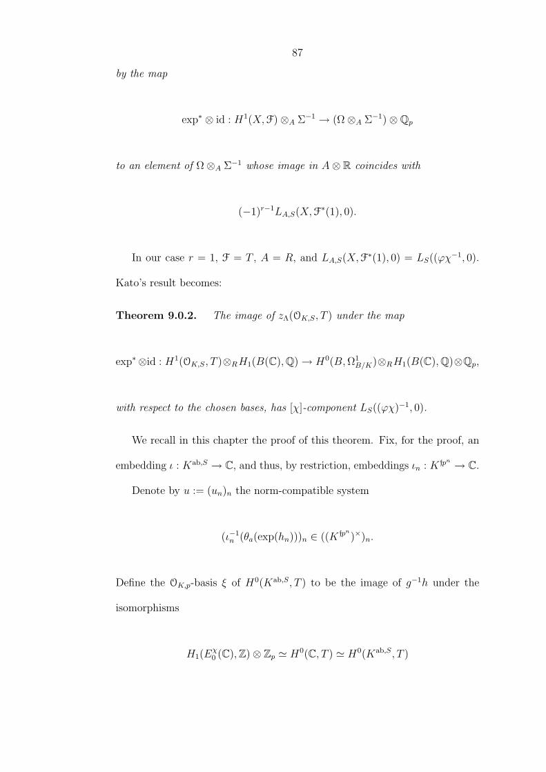
87
by the map
exp∗ ⊗ id : H1(X,F)⊗A Σ−1 → (Ω⊗A Σ−1)⊗Qp
to an element of Ω⊗A Σ−1 whose image in A⊗ R coincides with
(−1)r−1LA,S(X,F∗(1), 0).
In our case r = 1, F = T , A = R, and LA,S(X,F∗(1), 0) = LS((ϕχ
−1, 0).
Kato’s result becomes:
Theorem 9.0.2. The image of zΛ(OK,S, T ) under the map
exp∗⊗id : H1(OK,S, T )⊗RH1(B(C),Q)→ H0(B,Ω1B/K)⊗RH1(B(C),Q)⊗Qp,
with respect to the chosen bases, has [χ]-component LS((ϕχ)−1, 0).
We recall in this chapter the proof of this theorem. Fix, for the proof, an
embedding ι : Kab,S → C, and thus, by restriction, embeddings ιn : K fpn → C.
Denote by u := (un)n the norm-compatible system
(ι−1n (θa(exp(hn)))n ∈ ((K fpn)×)n.
Define the OK,p-basis ξ of H0(Kab,S, T ) to be the image of g−1h under the
isomorphisms
H1(Eχ0 (C),Z)⊗ Zp ' H0(C, T ) ' H0(Kab,S, T )

88
(where the right-hand isomorphism is induced by ι). Let ξn = π−nξ mod T ∈
V/T . Then the Coleman power series gu,ξ associated to u and ξ is the function
z 7→ θa(z + ι−1(exp(g−1h)))
on Eχ0 .
Fix n for the rest of the proof. Define s ∈ H1(K fpn , T∨(1)) to be the image
of u under
lim←−m
(K fpn)× // lim←−m
H1(K fpn ,Zp(1))
∪(ξm)∨m
lim←−m
H1(K fpn , T∨(1)/πm)
'
lim←−m
H1(K fpn , T∨(1)/πm)traceoo
H1(K fpn , T∨(1))
.
We will shortly apply the
Theorem 9.0.3 (Explicit Reciprocity Law). ([13], II, 2.1.7) The function
exp∗ : H1(K fpn , T∨(1))→ coLie(Eχ0 )⊗OK K
fpn
sends s to
π−nω ⊗((
d
ω
)log(ϕ−n(gu,ξ))
)(ξn)
(Here ω can be taken to be any OK-basis of coLie(Eχ0 ).)
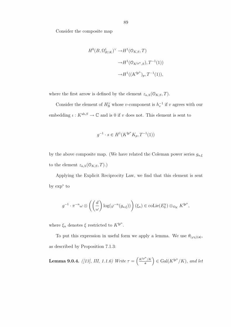
89
Consider the composite map
H0(B,Ω1B/K)∨ →H1(OK,S, T )
→H1(OKfpn ,S), T−1(1))
→H1((K fpn)p, T−1(1)),
where the first arrow is defined by the element za,Λ(OK,S, T ).
Consider the element of H∨B whose v-component is h−1
v if v agrees with our
embedding ι : Kab,S → C and is 0 if v does not. This element is sent to
g−1 · s ∈ H1(K fpnKp, T−1(1))
by the above composite map. (We have related the Coleman power series gu,ξ
to the element za,Λ(OK,S, T ).)
Applying the Explicit Reciprocity Law, we find that this element is sent
by exp∗ to
g−1 · π−nω ⊗((
d
ω
)log(ϕ−n(gu,ξ))
)(ξn) ∈ coLie(Eχ
0 )⊗OK Kfpn ,
where ξn denotes ξ restricted to K fpn .
To put this expression in useful form we apply a lemma. We use θ(ϕχ)(a),
as described by Proposition 7.1.3:
Lemma 9.0.4. ([13], III, 1.1.6) Write τ =(Kfpn/K
a
)∈ Gal(K fpn/K), and let

90
α = exp(hn) ∈ (Eχ0 )fpn(C) = (Eχ
0 )fpn(Kpn), σ ∈ Gal(K fpn/K). The value of
(d
ω
)log(θ(ϕχ)(a))
at σα is equal to
(∫hn
ω
)−1
·
(N(a)Lσ-part((ϕχ)−1, 0)− (ϕχ)(a)Lστ-part((ϕχ)−1, 0)
).
Choose a ≡ 1( mod f), so that τ = 1 and the above expression is simplified.
The image of za,Λ(OK,S, T ) we wish to ascertain is
g−1 · π−nω ⊗(∫
hn
ω
)−1
·
(N(a)− (ϕχ)(a)
)LS((ϕχ)−1, 0)
It follows that the image of
zΛ(OK,S, T ) =(N(a)−N(a)χT (σa)
−1)−1
za,Λ(OK,S, T )
is
g−1 · π−nω ⊗(∫
hn
ω
)−1
· LS((ϕχ)−1, 0)
=g−1 · π−nω ⊗(∫
π−ng−1h
ω
)−1
· LS((ϕχ)−1, 0),
=ω ⊗(∫
h
ω
)−1
· LS((ϕχ)−1, 0),
=c+[χ] · LS((ϕχ)−1, 0)
=c+[χ] · LS(ϕχ, 1).

91
This proves Theorem 9.0.2.

92
Chapter 10
Examples.
In this chapter we will find examples, or show the existence of examples, of
elliptic curves to which the our main theorem applies.
We search for elliptic curves E/F , having complex multiplication by a
nonmaximal order O = Z + f · OK , for which the Mordell-Weil group E(F )
has rank 0.
We will make some simplifying assumptions:
Assumption 10.0.1.
• K has class number 1.
• f is a prime ≥ 3.
The field F contains the j-invariant of E. The ring class group is Gf :=
IfZfPf
, where If is the group of fractional ideals prime to f , Zf is the group of
principal ideals with a generator in Q ⊂ K, and Pf is the group of principal
ideals with a generator ≡ 1 mod f . The ring class field of O is a field Hf
such that Gal(Hf/K) ' Gf . The theory of complex multiplication shows that
we may take also:
• F = Hf .

93
10.1 Elliptic curves with rank 0.
Note 10.1.1. If E/F and E0/F are two elliptic curves isogenous over F , then
L(E/F, s) = L(E0/F, s).
We have the following theorem of Coates and Wiles ([5]), a generalization
of a result of Arthaud:
Theorem 10.1.2. If rank(E0(F )) ≥ 1 then L(E0/F, 1) = 0.
Accordingly, we search for elliptic curves E0 for which
L(E0/F, 1) 6= 0.
Then we will try to show the existence of elliptic curves E/F , isogenous over
F , with complex multiplication by O = Z + f · OK .
10.2 Elliptic curves with complex multiplica-
tion by a nonmaximal order.
Suppose E0/K is an elliptic curve with complex multiplication by OK . There
exists an elliptic curve E/K, with complex multiplication by O, fitting into
the short exact sequence
0 // C // E0// E // 0 ,

94
with C finite.
Theorem 10.2.1. E is defined over Hf .
To prove this theorem we use the following
Lemma 10.2.2. There exists a short exact sequence
0 // TfE0// TfE // C // 0.
Proof of lemma. For each n ≥ 1, we have the diagram, with exact rows and
columns:
0
0
E0,fn
//
Efn //
C ′n
// 0
0 // C //
·fn
E0//
·fn
E //
·fn
0
0 // C // E0//
E //
0
0 0
The leftmost vertical map is 0 since C is f -torsion. By diagram-chasing, we
get an isomorphism C ′n → C. Chasing the diagram
E0,fn//
·f
Efn //
·f
C ′n
// 0
E0,fn−1 //
Efn−1 //
C ′n−1
// 0
0 0

95
shows that there is an isomorphism C ′n → C ′
n−1 which is compatible with the
isomorphisms C ′n → C and C ′
n−1 → C constructed above, in that the diagram
C ′n
'@
@@@@
@@@
' // C ′n−1
'zz
zzzz
zz
C
commutes. Then, taking the projective limit over diagrams
E0,fn//
·f
Efn //
·f
C ′n
//
0
E0,fn−1 // Efn−1 // C ′n−1
// 0,
we conclude that there is an exact sequence
0 // TfE0// TfE // C // 0.
Proof of Theorem 10.2.1. Consider the action of OK,f upon TfE0. It gives
rise to a representation
Zf [Gal(K/K)]→ O×K,f .
The image of
Zf [Gal(K/Hf )]
lies in (Zf + fOK,f )×. Therefore, Gal(K/Hf ) acts on TfE, compatibly with

96
the Gal(K/Hf )-action on TfE0. As a result of the exact sequence
0 // C // E0// E // 0 ,
Gal(K/Hf ) acts on C. The short exact sequence
0 // TfE0// TfE // C // 0
from Lemma 10.2.2 illustrates that C is Gal(K/Hf )-stable. Consequently, we
see from the previous exact sequence
0 // C // E0// E // 0
that E is also Gal(K/Hf )-stable. The result follows.
Our strategy will be to find ring class fields Hf and elliptic curves E0 over
F := Hf with
L(E0/F, 1) 6= 0.
These will be examples of rank-0 elliptic curves, to which Gross’ Conjecture
applies. Moreover, this will show the existence of rank-0 elliptic curves E with
nonmaximal endomorphism ring, to which only the more general Burns–Flach
Conjecture applies.
By Theorem 10.2.1, we may as well search for E0 with complex multipli-
cation by OK . We will in fact use curves E0 which are defined over K.
Write, as before, ϕ for a Grossencharacter of K, which when pre-composed
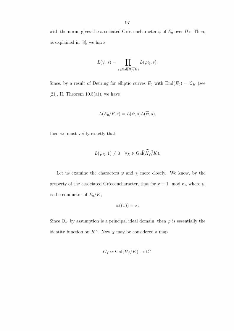
97
with the norm, gives the associated Grossencharacter ψ of E0 over Hf . Then,
as explained in [8], we have
L(ψ, s) =∏
χ∈ Gal(Hf/K)
L(ϕχ, s).
Since, by a result of Deuring for elliptic curves E0 with End(E0) = OK (see
[21], II, Theorem 10.5(a)), we have
L(E0/F, s) = L(ψ, s)L(ψ, s),
then we must verify exactly that
L(ϕχ, 1) 6= 0 ∀χ ∈ Gal(Hf/K).
Let us examine the characters ϕ and χ more closely. We know, by the
property of the associated Grossencharacter, that for x ≡ 1 mod c0, where c0
is the conductor of E0/K,
ϕ((x)) = x.
Since OK by assumption is a principal ideal domain, then ϕ is essentially the
identity function on K×. Now χ may be considered a map
Gf ' Gal(Hf/K)→ C×

98
Lemma 10.2.3. Gf is a group of order
2Φ(f)
φ(f)w,
where w = |O×K |, φ is Euler’s φ-function, and Φ is its obvious analog defined
on ideals of OK.
(A more precise description of this group will be given for examples we
find.)
Proof. First,
Gf =If
ZfPf' (OK/f)×
(Z/f)×im(O×K).
Consider the archimedean absolute value. We observe that 1+f ·OK intersects
the unit circle at only 1 point if f > 2, which is true here by assumption.
Therefore, the group homomorphism O×K → (OK/f)× is an injection, and
|im(O×K)| = |O×
K | = w. Since there are two roots of unity in Z×, the image of
(Z/f)× in (OK/f)×
im(O×K)has order φ(f)
2. Since
∣∣∣∣(OK/f)×
im(O×K)
∣∣∣∣ =Φ(f)
w,
the order of
(OK/f)×
(Z/f)×im(O×K)
is
2Φ(f)
φ(f)w,
as desired.

99
10.3 A first attempt.
Here we examine a first and mostly unsuccessful attempt to find examples.
We also explain why many of the curves of the class searched, can be ruled
out by theory alone.
Use K = Q(i), which has class number 1. If f ≡ 1 mod 4, then f is split
in K, and |Gf | = 2(f−1)2
4(f−1)= f−1
2. If f ≡ 3 mod 4, then f is inert in K, and
|Gf | = 2(f2−1)4(f−1)
= f+12
.
Consider the Gauss curve y2 = x3 − x, which we denote E0. It has
abelian torsion, so that the above considerations for ψ apply. If we knew
that L(ϕχ, 1) 6= 0 for all χ ∈ Gf , then we would be guaranteed the existence
of an elliptic curve E, defined over Hf , with complex multiplication by exactly
Z + f · OK and rankZE(Hf ) = 0.
As a preliminary search, a necessary (though insufficient) condition was
checked. The L-function satisfies the functional equation
Λ(ϕχ, s) = T (ϕχ)Λ(ϕχ, 2− s),
where
Λ(ϕχ, s) = (DN(ϕχ))s2 (2π)−sΓ(s)L(ϕχ, s),
where N(ϕχ) ∈ N is the norm of the conductor c(ϕχ) (an ideal of OK) and D
is the discriminant of K. And T (ϕχ) is related to the root number W (ϕχ) by
T (ϕχ) = −i W (ϕχ)√N(ϕχ)
.

100
Since E0 is defined over Q, then ϕ is anticyclotomic, i.e., ϕ(n) = ϕ(n). The
same is true of χ. On the ideals of Z, χ is trivial (since all ideals of Z represent
the trivial class in the ring class group). The Grossencharacter ϕ satisfies
ϕ((a)) = a for a ≡ 1 mod (1 + i)3,
so that for a ∈ Z, ϕ((a)) = a for a ≡ 1 mod 4 and ϕ((a)) = −a for a ≡ 3
mod 4. This means that the value of ϕ is real on the ideals of Z. Thus
L(ϕχ, 1) = L(ϕχ, 1), which means that any root numberW (ϕχ) being unequal
to 1 will force the L-value to be 0.
For each prime f between 3 and 250, the root number W (ϕχ) was checked
numerically for all characters χ of Gf . W (ϕχ) was found to be -1 for at least
one χ for each f 6= 3. This can in fact be proven for all f > 3:
Proposition 10.3.1. Let f be any prime > 3. Then there exists χ ∈ Gf such
that W (ϕχ) 6= 1.
Proof. We shall restrict our attention to nontrivial χ. We have as in Miyake
([16], 3.3.11), the formula for the root number of ϕχ:
W (ϕχ) = W (ϕ)W (χ)ϕ(cχ)
|ϕ(cχ)|χ(cϕ),
where cϕ and cχ are the respective conductors of ϕ and χ. Let us examine
the factors W (ϕ), W (χ), ϕ(cχ)
|ϕ(cχ)| , and χ(cϕ). We shall determine the first two,
and show that the fourth can be chosen, depending on the third, making the
whole product -1.

101
We know that W (ϕ) = 1 since the Gauss curve is a rank-0 elliptic curve.
Second, let us examine W (χ). The character χ is a character of the Galois
group of the extension F = Hf/K. Consider the representation
ResQKIndQ
Kχ
formed by induction and then restriction. It is
x 7→
χ(x) 0
0 χ(x)
.
Now since xx ∈ Z for x ∈ OK , and since the image of Z in Gf is trivial, then
χ(x)χ(x) = χ(xx) = 1,
so that χ is anti-cyclotomic (i.e., χ(x) = χ(x)). It follows that the character
associated to the representation
ResQKIndQ
Kχ

102
is
tr(ResQKIndQ
Kχ) =tr
χ(x) 0
0 χ(x)
=tr
χ(x) 0
0 χ(x)
=χ(x) + χ(x)
∈R.
One also checks that tr(IndQKχ)(x) ∈ R for x ∈ GQ\GK . The work of Frohlich
and Queyrut ([7]) tells us that for a real character which comes from a real
representation, the root number is 1. Though the representation IndQKχ is not
itself real, it is conjugate to a real representation. Thus its root number is also
1. Since the L-function is unchanged by induction or restriction of characters,
we see that W (χ) must be 1.
Next, we examine the factor ϕ(cχ)
|ϕ(cχ)| . Since the conductor of χ is f if χ is
nontrivial, then ϕ(cχ) ∈ Z, and the factor ϕ(cχ)
|ϕ(cχ)| is ±1 .
The class of cϕ = (1 + i)3 is of order exactly 2 in Gf since its square is
the class of the ideal (8), which is trivial, while the class of (1 + i)3 is itself
nontrivial. Therefore, there exists a character χ of Gf which has value −1 at
cϕ. Since f > 3, then Gf 6=< 1 + i >, so that there is a nontrivial character
of Gf which factors through Gf/ < 1 + i >.
103
Whether ϕ(cχ)
|ϕ(cχ)| is 1 or -1, we find a χ ∈ Gf for which the product
ϕ(cχ)
|ϕ(cχ)|χ(cϕ),
and thus the product
ϕ(cχ)
|ϕ(cχ)|χ(cϕ)W (ϕ)W (χ),
is -1. Thus, for f > 3, there exists χ ∈ Gf such that W (ϕχ) = −1.
The curve E0/H3 turned out to have non-zero L-value, and so E3 was the
lone example obtained from this search.
10.4 A second search.
A different class of curves was searched, yielding 15 elliptic curves over ring
class fields F := Hf with
L(E0/F, 1) 6= 0.
These are examples of rank-0 elliptic curves, to which Gross’ Conjecture ap-
plies. Moreover, this shows the existence of 15 rank-0 elliptic curves E with
nonmaximal endomorphism ring, to which only the more general Burns–Flach
Conjecture applies.
Here the Gauss curve E0 is replaced by a quartic twist thereof. Let E4,0
be given by the equation
y2 = x3 − (1 + 4i)x.

104
This curve is isomorphic to the Gauss curve over F (4√
1 + 4i), using the co-
ordinate change (x, y) = (β2x′, β3y′), where β = 4√
1 + 4i. Since the Gauss
curve y2 = x3 − x has abelian torsion, then E4,0 does also. If we knew that
L(ϕ′χ, 1) 6= 0 for all χ ∈ Gf , where ϕ′ is the Grossencharacter of E4,f , then we
would be guaranteed the existence of an elliptic curve E4,f , defined over Hf ,
with complex multiplication by exactly Z + f · OK .
The Grossencharacter of E4,0 is ϕ′ = ϕε, where ε is the character associated
to the quartic twist E0 7→ E4,0. We have
ϕ′((α)) =
(1 + 4i
α
)4
α, α ≡ 1 mod (1 + i)3.
(See [12], Chapter 19, Theorem 5.) The conductor of ε is 1+4i, which is prime
to the conductor of ϕ, and to the conductor of χ if f 6= 17. In this case, the
root number of ξ = ϕ′χ can be calculated using the formula
W (ϕ′χ) =ϕ′(cχ)
|ϕ′(cχ)|ε(cϕ′)W (ϕ′)W (χ),
where the root number of ϕ′ = ϕε is calculated using the formula
W (ϕε) =ϕ(cε)
|ϕ(cε)|ε(cϕ)W (ϕ)W (ε).
The values of L(ϕ′χ, 1) were checked for all ring class characters χ, for all
primes f between 3 and 61, excluding 17. The values L(ϕ′χ, 1) were found
all to be non-zero, except when f = 5 and χ was the non-trivial character of
the two-element group G5. In this case, L(ϕ′χ, 1) appeared to be zero, though

105
this could not be deduced from the numerical calculations. In any case, it was
determined that E4,0/Hf had non-zero L-value for the following 15 values of
f :
3, 7, 11, 13, 19, 23, 29, 31, 37, 41, 43, 47, 53, 59, 61.
Thus there exists an example E4,f for each of these values of f .
10.5 The code.
Here we give the code used in PARI to find the examples. With some mod-
ification, many other similar classes of elliptic curves could be searched. Ex-
planation is given interspersed with the code. Comments generally follow the
line or lines to which they refer.
bnf=bnfinit(y^2+1);
Initializes the number field ‘bnf’= Q(i).
bnr2=bnrinit(bnf,[1,4]~,1);
Initializes ‘bnr2’, which is Q(i) with the structure of the ray class group mod-
ulo 1 + 4i.
initialize(f)=
Initializes the data involving f =‘eff’.
eff=f;

106
Sets f , called ‘eff’.
bnr=bnrinit(bnf,eff,1);
Initializes ‘bnr’, which is Q(i) with the structure of the ray class group modulo
f .
bnr3=bnrinit(bnf,eff*[1,4]~,1);
Initializes ‘bnr3’, which is Q(i) with the structure of the ray class group mod-
ulo f(1 + 4i).
prim=znprimroot(eff);
for(index=1,eff,
if(prim==Mod(index,eff),
prim=index
)
);
prim=bnrisprincipal(bnr,prim)[1];
Sets a generator ‘prim’ of (Z/fZ)∗.
chi=vector(length(bnr.clgp[2]));
Sets χ to be the trivial character.
h1generator(bnf,ideal)=
Extracts a generator of ‘ideal’ in ‘bnr’, assuming the class number of ‘bnr’ is
1.
dec=factor(idealnorm(bnf,ideal));

107
gen=1;
for(index=1,matsize(dec)[1],
fac1=[dec[index,1],0]~;
fac2=[1,0]~;
for(a=1,sqrt(dec[index,1]),
for(b=1,a,
if(a^2+b^2==dec[index,1],
fac1=[a,b]~;
fac2=[a,-b]~;
)
)
);
gen=nfeltmul(bnf,gen,
nfeltpow(bnf,fac1,idealval(bnf,
ideal,idealfactor(bnf,fac1)[1,1]))
);
if(fac1!=[1,1]~& fac2!=[1,0]~,
gen=nfeltmul(bnf,gen,
nfeltpow(bnf,fac2,idealval(bnf,
ideal,idealfactor(bnf,fac2)[1,1]))
);
);
);
gen

108
phieval(ideal)=
Evaluates the character ϕ =‘phi’ (factor of the Grossencharacter) at ‘ideal’,
given by a generator, expressed as a column vector on the integral basis.
for(o=0,3,
if(nfeltmod(bnf,
nfeltmul(bnf, ideal,nfeltpow(bnf,[0,1]~,o))-[1,0]~,
nfeltpow(bnf,[1,1]~,3))
==[0,0]~,
ideal=nfeltmul(bnf, ideal,nfeltpow(bnf,[0,1]~,o));
);
);
if(nfeltmod(bnf,ideal,[1,1]~)==[0,0]~,
ideal=[0,0]~;
);
ideal[1]+ideal[2]*I
epsiloneval(ideal)=
Evaluates the character ε =‘epsilon’, associated to the quartic twist of E by
1 + 4i, at ‘ideal’. We know the character is either [1] or [3] as a character of
the cyclic 4-group ‘bnr2.clgp’, and, twisting three times if necessary, we may

109
assume without loss of generality that it is [1].
if(idealnorm(bnr2,idealcoprime(bnr2,[1,4]~,ideal))!=1,
0,
exp(2*Pi*I*bnrisprincipal(bnr2,ideal)[1][1]
*1/bnr2.clgp[2][1])
)
rnepsilon=bnrrootnumber(bnr2,[1]);
Calculates the (fixed) root number of ε =‘epsilon’.
phiprimeeval(ideal)=
Evaluates ϕ′ =‘phiprime’= ϕε at ‘ideal’.
phieval(ideal)*epsiloneval(ideal)
cophiprime=nfeltmul(bnf,[1,4]~,nfeltpow(bnf,[1,1]~,3));
Calculates the conductor of ϕ′ =‘phiprime’= ϕε.
rnphiprime=(1+4*I)/sqrt(17)
*epsiloneval(nfeltpow(bnf,[1,1]~,3))
*1*rnepsilon;

110
Calculates the (fixed) root number of ‘phiprime’=‘phi’·‘epsilon’. (At 1+4i, the
conductor of ‘epsilon’, ‘phi’ takes the value 1+4i.)
chieval(ideal)=
Evaluates the character χ =‘chi’ of the ray class group modulo f , at ideal.
if(idealnorm(bnr,bnrconductorofchar(bnr,chi))==1,
1,
if(idealnorm(bnr,idealcoprime(bnr,
bnrconductorofchar(bnr,chi),ideal))!=1,
0,
exp(2*Pi*I*(
sum(index=1,length(bnr.clgp[2]),
bnrisprincipal(bnr,ideal)[1][index]*chi[index]
/bnr.clgp[2][index]
)
))
)
)
xieval(ideal)=
Evaluates the character ξ =‘xi’= ϕ′χ = ϕεχ at the ideal generated by ‘ideal’.

111
phiprimeeval(ideal)*chieval(ideal)
rnxi()=
This calculates the root number (varying with χ) of ξ =‘xi’= φ′χ = φεχ.
cochi=h1generator(bnr,bnrconductorofchar(bnr,chi));
fact=phiprimeeval(cochi);
if(fact==0,0,
fact/sqrt(norm(fact))
*chieval(cophiprime)
*rnphiprime
*bnrrootnumber(bnr,chi)
)
isring(upsilon)=
Tests whether ‘upsilon’, a character of the ray class group modulo f (‘bnr.clgp’),
factors through the ring class group modulo f , and thus is a valid χ to con-
sider. Uses the constant ‘prim’, which is a generator of (Z/fZ)∗ , expressed
as an element of ‘bnr.clgp’.
if(length(bnr.clgp[2])==1,
upsilon[1]*prim[1]%(bnr.clgp[2][1])==0,

112
(upsilon[1]*prim[1]*bnr.clgp[2][2]
+upsilon[2]*prim[2]*bnr.clgp[2][1])
%(bnr.clgp[2][1]*bnr.clgp[2][2])==0;
Tests whether ‘upsilon’ factors through the quotient by (Z/fZ)∗ ,i.e., whether
it gives character on the ring class group as well as the ray class group.
)
getapbp(p)=
Sets ap =‘ap’ and bp =‘bp’ for the modular form.
if(idealprimedec(bnr,p)[1][4]==2,
ap=0;
bp=-xieval([p,0]~);
);
if(idealprimedec(bnr,p)[1][3]==2,
for(i=1,sqrt(p),
for(j=1,i,
if(i^2+j^2==p,
ap=xieval([i,j]~);
bp=0
);
);
);

113
);
if(length(idealprimedec(bnr,p))==2,
for(i=1,sqrt(p),
for(j=1,i,
if(i^2+j^2==p,
v1=xieval([i,j]~);
v2=xieval([i,-j]~);
ap=(v1+v2);
bp=(v1*v2)
);
);
);
);
add(n,P,y,z)=
This function calls itself, and is the heart of the Gross–Buhler recursion.
Sum=Sum+y*expq^n/n;
forprime(p=2,min(P,bound/n),
getapbp(p);
x=y*ap;
if(p==P,x=x-z*bp);
add(p*n,p,x,y);

114
)
GB(bound)=
f1=expq;
a1=1;
Sum=a1*f1;
forprime(p=2,bound,
getapbp(p);
add(p,p,ap,1);
);
Sum
The preceding two functions comprise the algorithm of Gross and Buhler,
as described in [1]. This algorithm can be described as “computationally min-
imal” in the sense that, using the known relations between the various an and
bn (surely the most efficient way to calculate the terms), the minimum num-
ber of them necessary for the rest to be calculated, are kept in memory at once.
Lval(xx,bound)=

115
This function approximates the L-value L(ξ, 1), using the formula
L(ξ, 1) =∞∑n=1
anne− 2πnx√
N + T (ξ)∞∑n=1
annne
− 2πn
x√N ,
where N = |D|N(ξ), D being the discriminant of K. The computaion uses
the cutoff point x =‘xx’ ≈ 1, and ‘bound’ terms of each series. Varying x does
not change the infinite sum, of course, and this was used as a way to check
the correctness of the calculation.
expq=exp(-2*Pi/sqrt(4*2^3*17*idealnorm(bnf,
bnrconductorofchar(bnr,chi)))*xx);
term1=GB(bound);
expq=exp(-2*Pi/sqrt(4*2^3*17*idealnorm(bnf,
bnrconductorofchar(bnr,chi)))*(1/xx));
term2=conj(GB(bound));
term1+rnxi*term2
multichi1()=
Checks the L-value for fixed f and all possible χ, for cyclic ray class group
modulo f . Note that in all cases the ring class group modulo f is cyclic, but
it is more convenient here to examine the characters of the ray class group,
finding the L-value only for those which factor through the ring class group.
(In some cases, the ray class group is not cyclic.)

116
indicator=1;
for(a=0,bnr.clgp[1]-1,
if((isring([a])==1)&(indicator==1),
chi=[a];
if(truncate(norm(1000*Lval(1,500)))==0,
indicator=0
);
);
);
if(indicator==1,
print("GOOD f=" eff ),
print("BAD f=" eff)
)
Prints “GOOD” if Ef is an elliptic curve of the desired type, and “BAD” oth-
erwise.
multichi2()=
Checks the L-value for fixed f and all possible χ, for ray class group modulo f
with 2 cyclic components. Again, only those characters which factor through
the ring class group are considered.
for(a=0,bnr.clgp[2][1]-1,

117
for(b=0,bnr.clgp[2][2]-1,
if((isring([a,b])==1)&(indicator==1),
chi=[a,b];
if(truncate(norm(1000*Lval(1,500)))==0,
indicator=0
);
);
);
);
if(indicator==1,
print("GOOD f=" eff ),
print("BAD f=" eff)
)
Prints “GOOD” if Ef is an elliptic curve of the desired type, and “BAD” oth-
erwise.
multieff(lower,upper)=
Checks the L-value for all (prime) f from ‘lower’ to ‘upper’. Note that for
all f ≡ 3 mod 4, f is inert, which implies that the ray class group modulo
f is cyclic. For all f > 5,≡ 1 mod 4, f is non-inert and the ray class group
has two cyclic components. For f=5, the ray class group is cyclic. We do not
wish to examine f = 2 or 17 because they are not prime to the conductors of
φ and ε, respectively. Thus ranges [‘lower’,‘upper’] are chosen, when this code

118
is used, which exclude 2 and 17.
forprime(index=lower,upper,
initialize(index);
if(length(bnr.clgp[2])==1,
multichi1,
multichi2
);
);
119
Bibliography
[1] Buhler, J. and Gross, B., “Arithmetic on elliptic curves with complex
multiplication. II.” Invent. Math. 79 (1985), 223—251.
[2] Burns, D. and Flach, M., “Motivic L-functions and Galois module struc-
tures.” Math. Ann. 305 (1996), 65—102.
[3] Burns, D. and Flach, M., “On Galois structure invariants associated to
Tate motives.” American Journal of Mathematics 120 (1998), 1343—
1397.
[4] Burns, D. and Flach, M., “Tamagawa numbers for motives with (non-
commutative) coefficients.” Documenta Math. 6 (2001), 501—570.
[5] Coates, J. and Wiles, A., “On the Conjecture of Birch and Swinnerton-
Dyer.” Invent. Math. 39 (1977), 223—251.
[6] Fontaine, J.-M. and Perrin-Riou, B., “Autour des conjectures de Bloch
et Kato: cohomologie galoisienne et valeurs de fonctions L.” (French)
(Seattle, WA, 1991), 599—706, Proc. Sympos. Pure Math., 55, Part 1,
Amer. Math. Soc., Providence, RI, 1994.
120
[7] Frohlich A. and Queyrut, J., “On the functional equation of the Artin L-
function for characters of real representations.” Invent. Math. 20 (1973),
125—138.
[8] Goldstein, C. and Schappacher, N., “Series d’Eisenstein et fonctions L de
courbes elliptiques multiplication complexe.” (French) J. Reine Angew.
Math. 327 (1981), 184—218.
[9] Gross, B., “On the conjecture of Birch and Swinnerton-Dyer for elliptic
curves with complex multiplication.” (Cambridge, Mass., 1981), 219—
236, Progr. Math., 26, Birkhauser, Boston, Mass., 1982.
[10] Gross, B., Arithmetic on elliptic curves with complex multiplication.
Springer Lecture Notes Math. 776.
[11] Grothendieck, A., “Modeles de Neron et monodromie.” Expose IX, SGA
7I, Springer–Verlag, 1972.
[12] Ireland, K. and Rosen, M,, A Classical Approach to Modern Number The-
ory. Springer GTM 84, 1982.
[13] Kato, K., Lectures on the approach to Iwasawa theory for Hasse-Weil L-
functions via BdR. I. (Trento, 1991), 50—163, Lecture Notes in Math.,
1553, Springer, Berlin, 1993.
[14] Knudsen, F. and Mumford, D., “The projectivity of the moduli space of
stable curves I: Preliminaries on ‘det’ and ‘Div’.” Math. Scand 39 (1976)
19—55.

121
[15] Matsumura, H., Commutative Algebra. Benjamin Cummings, 1980.
[16] Miyake, T., Modular Forms. Springer–Verlag, 1989.
[17] Rubin, K., “The ‘main conjectures’ of Iwasawa theory for quadratic imag-
inary fields.” Invent. Math. 103 (1991), no. 1, 25—68.
[18] Rubin, K., Euler Systems. Annals of Mathematics Studies, 147. Hermann
Weyl Lectures. The Institute for Advanced Study. Princeton University
Press, Princeton, NJ, 2000.
[19] de Shalit, E., Iwasawa theory of elliptic curves with complex multiplica-
tion. Orlando: Academic Press (1987).
[20] Silverman, J. H., The Arithmetic of Elliptic Curves. New York: Springer-
Verlag (1986).
[21] Silverman, J. H., Advanced Topics in the Arithmetic of Elliptic Curves.
New York: Springer-Verlag (1994).


![ON THE BIRCH–SWINNERTON-DYER QUOTIENTS MODULO …tomlr.free.fr/Math%E9matiques/Elliptic%20curves%20and%20... · 2009-02-17 · arXiv:math/0610290v2 [math.NT] 9 Apr 2007 ON THE BIRCH–SWINNERTON-DYER](https://img.pdfslide.us/doc/110x75/5fa012c8cdd97f33b168be40/on-the-birchaswinnerton-dyer-quotients-modulo-tomlrfreefrmathe9matiqueselliptic20curves20and20.jpg)


![On the conjecture of Birch and Swinnerton-Dyer for Abelian ... · Birch-Swinnerton-Dyer and the Artin-Tate conjecture for the base a curve, see Gordon’s PhD thesis [Gor79]. Let](https://img.pdfslide.us/doc/110x75/5f05f0fd7e708231d4157de5/on-the-conjecture-of-birch-and-swinnerton-dyer-for-abelian-birch-swinnerton-dyer.jpg)

![VISIBLE EVIDENCE FOR THE BIRCH AND SWINNERTON-DYER ... · Birch and Swinnerton-Dyer conjecture for modular abelian varieties of dimension greaterthan2(see[FpS+01]fordimension2). This](https://img.pdfslide.us/doc/110x75/5f05f0f87e708231d4157dc8/visible-evidence-for-the-birch-and-swinnerton-dyer-birch-and-swinnerton-dyer.jpg)