The Concept of NSO SPRING...and more

Luca Bertello

US National Solar ObservatoryBoulder, Colorado

Sanjay Gosain, Frank Hill, Alexei A. Pevtsov

SONG2018 Workshop Tenerife, Spain - October 23 - 26, 2018

1 / 31

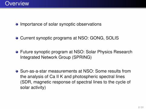
Overview

Importance of solar synoptic observations

Current synoptic programs at NSO: GONG, SOLIS

Future synoptic program at NSO: Solar Physics ResearchIntegrated Network Group (SPRING)

Sun-as-a-star measurements at NSO: Some results fromthe analysis of Ca II K and photospheric spectral lines(SDR, magnetic response of spectral lines to the cycle ofsolar activity)

2 / 31

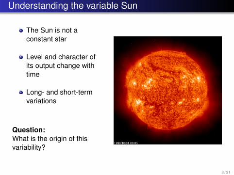
Understanding the variable Sun

The Sun is not aconstant star

Level and character ofits output change withtime

Long- and short-termvariations

Question:What is the origin of thisvariability?

3 / 31

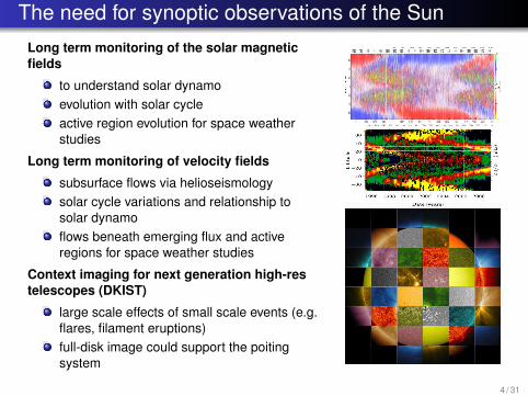
The need for synoptic observations of the Sun

Long term monitoring of the solar magneticfields

to understand solar dynamoevolution with solar cycleactive region evolution for space weatherstudies

Long term monitoring of velocity fields

subsurface flows via helioseismologysolar cycle variations and relationship tosolar dynamoflows beneath emerging flux and activeregions for space weather studies

Context imaging for next generation high-restelescopes (DKIST)

large scale effects of small scale events (e.g.flares, filament eruptions)full-disk image could support the poitingsystem

4 / 31

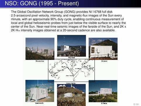
NSO: GONG (1995 - Present)The Global Oscillation Network Group (GONG) provides Ni I 6768 full disk2.5-arcsecond pixel velocity, intensity, and magnetic-flux images of the Sun everyminute, with an approximate 90% duty cycle, enabling continuous measurement oflocal and global helioseismic probes from just below the visible surface to nearly thecenter of the Sun. Near-real-time seismic images of the farside of the Sun, and 2K x2K Hα intensity images obtained at a 20-second cadence are also available.

5 / 31

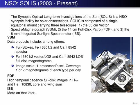
NSO: SOLIS (2003 - Present)

The Synoptic Optical Long-term Investigations of the Sun (SOLIS) is a NSOsynoptic facility for solar observations. SOLIS is composed of a singleequatorial mount carrying three telescopes: 1) the 50 cm VectorSpectroMagnetograph (VSM), 2) the 14 cm Full-Disk Patrol (FDP), and 3) the8 mm Integrated Sunlight Spectrometer (ISS).

VSMData products include, among others:

Full-Stokes, Fe I 6301/2 and Ca II 8542spectraFe I 6301/2 vector/LOS and Ca II 8542 LOSfull-disk magnetogramsImage scale: 1-arcsecond/pixel. Coverage:1 or 2 magnetograms of each type per day.

FDPHigh temporal cadence full-disk images in H-αand He I 10830, core and wing sumISSMore on that later...

6 / 31

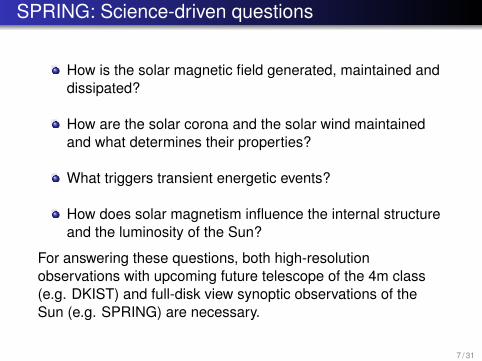
SPRING: Science-driven questions

How is the solar magnetic field generated, maintained anddissipated?

How are the solar corona and the solar wind maintainedand what determines their properties?

What triggers transient energetic events?

How does solar magnetism influence the internal structureand the luminosity of the Sun?

For answering these questions, both high-resolutionobservations with upcoming future telescope of the 4m class(e.g. DKIST) and full-disk view synoptic observations of theSun (e.g. SPRING) are necessary.

7 / 31

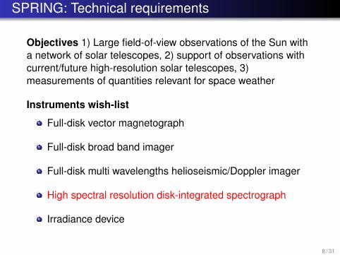
SPRING: Technical requirements

Objectives 1) Large field-of-view observations of the Sun witha network of solar telescopes, 2) support of observations withcurrent/future high-resolution solar telescopes, 3)measurements of quantities relevant for space weather

Instruments wish-list

Full-disk vector magnetograph

Full-disk broad band imager

Full-disk multi wavelengths helioseismic/Doppler imager

High spectral resolution disk-integrated spectrograph

Irradiance device

8 / 31

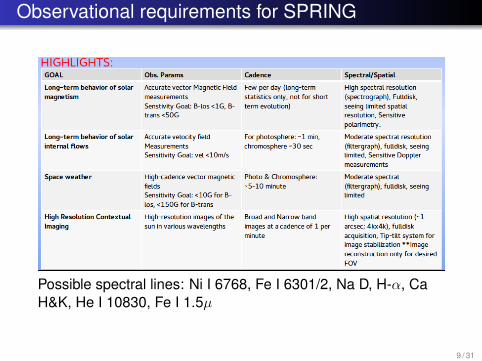
Observational requirements for SPRING

Possible spectral lines: Ni I 6768, Fe I 6301/2, Na D, H-α, CaH&K, He I 10830, Fe I 1.5µ

9 / 31

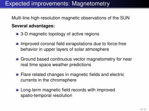
Expected improvements: Magnetometry

Multi-line high-resolution magnetic observations of the SUN

Several advantages:

3-D magnetic topology of active regions

Improved coronal field exrapolations due to force-freebehavior in upper layers of solar atmosphere

Ground based continuous vector magnetometry for nearreal time space weather predictions

Flare related changes in magnetic fields and electriccurrents in the chromsphere

Long-term magnetic field records with improvedspatio-temporal resolution

10 / 31

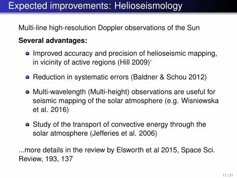
Expected improvements: Helioseismology

Multi-line high-resolution Doppler observations of the Sun

Several advantages:

Improved accuracy and precision of helioseismic mapping,in vicinity of active regions (Hill 2009)‘

Reduction in systematic errors (Baldner & Schou 2012)

Multi-wavelength (Multi-height) observations are useful forseismic mapping of the solar atmosphere (e.g. Wisniewskaet al. 2016)

Study of the transport of convective energy through thesolar atmosphere (Jefferies et al. 2006)

...more details in the review by Elsworth et al 2015, Space Sci.Review, 193, 137

11 / 31

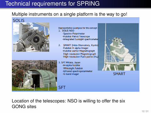
Technical requirements for SPRING

Multiple instruments on a single platform is the way to go!

Location of the telescopes: NSO is willing to offer the sixGONG sites

12 / 31

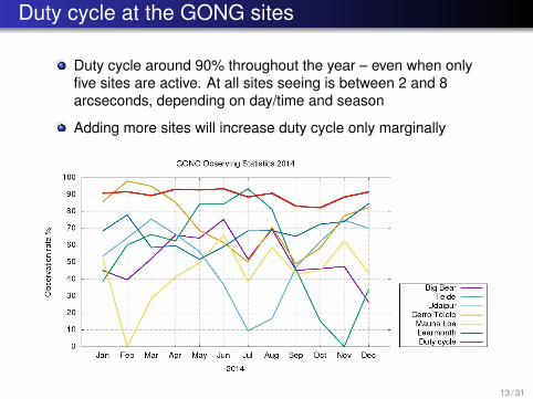
Duty cycle at the GONG sites

Duty cycle around 90% throughout the year – even when onlyfive sites are active. At all sites seeing is between 2 and 8arcseconds, depending on day/time and season

Adding more sites will increase duty cycle only marginally

13 / 31

TIME FOR SOME SCIENCE!

1) Sun-as-a-star in Ca II K

2) Response of photospheric lines tosolar activity

14 / 31

Importance of Sun-as-a-star measurements

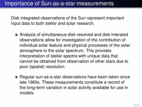
Disk integrated observations of the Sun represent importantinput data to both stellar and solar research.

Analysis of simultaneous disk-resolved and disk-interatedobservations allow for investigation of the contribution ofindividual solar feature and physical processes of the solaratmosphere to the solar spectrum. This providesinterpretation of stellar spectra with unique data thatcannot be obtained from observation of other stars due topoor (spatial) resolution.

Regular sun-as-a-star observations have been taken sincelate 1960s. These measurements constitute a record ofthe long-term variation in solar activity available for use inmodels.

15 / 31

Sun-as-a-star measurements at NSO

Ca II K-Line monitoring program at Sacramento Peak(November 1976 - September 2015). Seven K-lineparameters, including the 1-Å emission index.

Measurements by W. Livingston at Kitt Peak, fromNovember 1974 to July 2013.

Measurements with the SOLIS/ISS instrument (December2006 - ongoing). These measurements include the Ca IIK-line, from which nine different parameters are extracted(Bertello et al. 2012; Pevtsov et al. 2014).

16 / 31

NSO: SOLIS/ISS

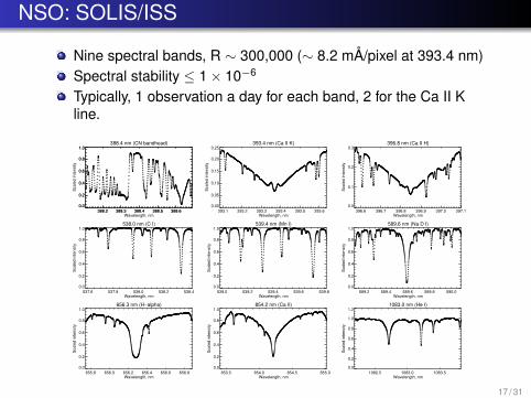
Nine spectral bands, R ∼ 300,000 (∼ 8.2 mÅ/pixel at 393.4 nm)Spectral stability ≤ 1× 10−6

Typically, 1 observation a day for each band, 2 for the Ca II Kline.

388.2 388.3 388.4 388.5 388.6

0.0

0.2

0.4

0.6

0.8

1.0388.4 nm (CN bandhead)

388.2 388.3 388.4 388.5 388.6Wavelength, nm

0.0

0.2

0.4

0.6

0.8

1.0

Sca

led

in

ten

sity

393.4 nm (Ca II K)

393.1 393.2 393.3 393.4 393.5 393.6Wavelength, nm

0.00

0.05

0.10

0.15

0.20

0.25

Sca

led

in

ten

sity

396.8 nm (Ca II H)

396.6 396.7 396.8 396.9 397.0 397.1Wavelength, nm

0.0

0.1

0.2

0.3

Sca

led

in

ten

sity

538.0 nm (C I)

537.6 537.8 538.0 538.2 538.4Wavelength, nm

0.0

0.2

0.4

0.6

0.8

1.0

Sca

led

in

ten

sity

539.4 nm (Mn I)

539.0 539.2 539.4 539.6 539.8Wavelength, nm

0.0

0.2

0.4

0.6

0.8

1.0

Sca

led

in

ten

sity

589.6 nm (Na D I)

589.2 589.4 589.6 589.8 590.0Wavelength, nm

0.0

0.2

0.4

0.6

0.8

1.0

Sca

led

in

ten

sity

656.3 nm (H−alpha)

655.8 656.0 656.2 656.4 656.6 656.8Wavelength, nm

0.0

0.2

0.4

0.6

0.8

1.0

Sca

led

in

ten

sity

854.2 nm (Ca II)

853.5 854.0 854.5 855.0Wavelength, nm

0.0

0.2

0.4

0.6

0.8

1.0

Sca

led

in

ten

sity

1083.0 nm (He I)

1082.5 1083.0 1083.5Wavelength, nm

0.0

0.2

0.4

0.6

0.8

1.0

1.2

Sca

led

in

ten

sity

17 / 31

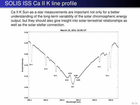
SOLIS ISS Ca II K line profileCa II K Sun-as-a-star measurements are important not only for a betterunderstanding of the long-term variability of the solar chromospheric energyoutput, but they should also give insight into solar-terrestrial relationships aswell as the solar-stellar connection.

March 15, 2011 16:00 UT

393.1 393.2 393.3 393.4 393.5 393.6Wavelength (nm)

0.00

0.05

0.10

0.15

0.20

0.25

0.30

Sca

led

Inte

nsi

ty

Fe I

Ti II

Fe I

Fe I

Fe I

K3

K2RK2V

K1RK1V

18 / 31

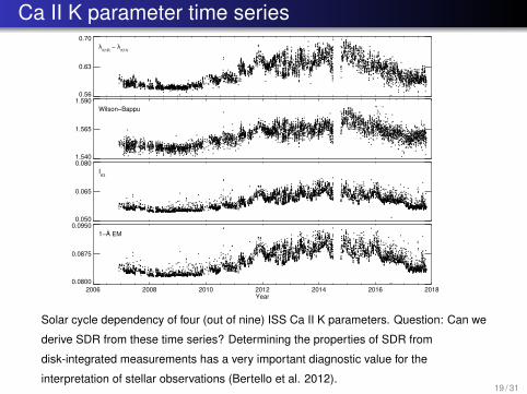
Ca II K parameter time series

2006 2008 2010 2012 2014 2016 2018Year

0.0800

0.0875

0.09501−Å EM

0.050

0.065

0.080IK3

1.540

1.565

1.590Wilson−Bappu

0.56

0.63

0.70λ

K1R − λ

K1V

Solar cycle dependency of four (out of nine) ISS Ca II K parameters. Question: Can we

derive SDR from these time series? Determining the properties of SDR from

disk-integrated measurements has a very important diagnostic value for the

interpretation of stellar observations (Bertello et al. 2012).19 / 31

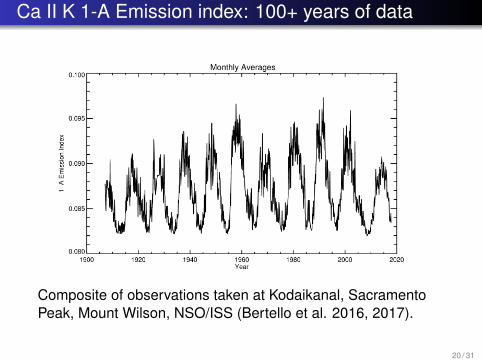
Ca II K 1-A Emission index: 100+ years of data

Composite of observations taken at Kodaikanal, SacramentoPeak, Mount Wilson, NSO/ISS (Bertello et al. 2016, 2017).

20 / 31

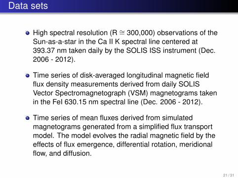
Data sets

High spectral resolution (R ∼= 300,000) observations of theSun-as-a-star in the Ca II K spectral line centered at393.37 nm taken daily by the SOLIS ISS instrument (Dec.2006 - 2012).

Time series of disk-averaged longitudinal magnetic fieldflux density measurements derived from daily SOLISVector Spectromagnetograph (VSM) magnetograms takenin the FeI 630.15 nm spectral line (Dec. 2006 - 2012).

Time series of mean fluxes derived from simulatedmagnetograms generated from a simplified flux transportmodel. The model evolves the radial magnetic field by theeffects of flux emergence, differential rotation, meridionalflow, and diffusion.

21 / 31

Data reduction: Irregularly sampled data

Time series is detrended (model or 4-th order B-spline)

Rejection of outliers from the time series, e.g. 3-σ rejection

Option #1: Lomb-Scargle periodogram and you are done (I hate it!)

Option #2: Resampling (I love it!)

Nearest Neighbor Resampling with the Slotting (NNRS)principle + (linear) interpolation for missing data.

A low-pass filter is applied to the data (R-E algorithm).

Prewhitening (AR model) is necessary to reduce thenon-stationary components of the signal.

Choice between FFT and MEM

22 / 31

Maximum entropy spectral estimator (MEM)

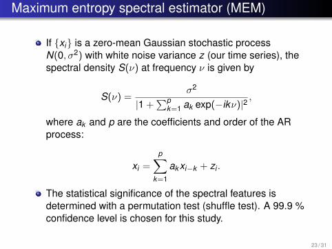
If {xi} is a zero-mean Gaussian stochastic processN(0, σ2) with white noise variance z (our time series), thespectral density S(ν) at frequency ν is given by

S(ν) =σ2

|1 +∑p

k=1 ak exp(−ikν)|2,

where ak and p are the coefficients and order of the ARprocess:

xi =

p∑k=1

akxi−k + zi .

The statistical significance of the spectral features isdetermined with a permutation test (shuffle test). A 99.9 %confidence level is chosen for this study.

23 / 31

Power spectra of full-length time series

0.000 0.005 0.010 0.015 0.020 0.025 0.030 0.035 0.040 0.045 0.050 0.055 0.060Frequency (cycles/day)

200.0 100.0 66.7 50.0 40.0 33.3 28.6 25.0 22.2 20.0 18.2 16.7

Period (days)

1−Å emission index

IK3

Wilson−Bappu

λK1R

− λK1V

MF 630.15 nm

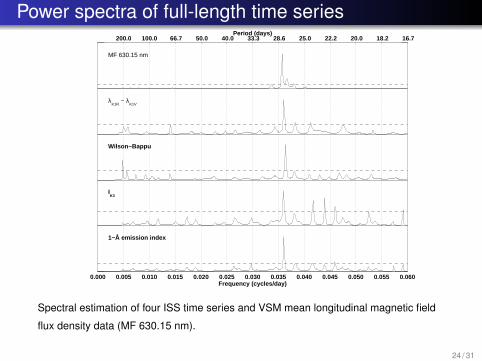
Spectral estimation of four ISS time series and VSM mean longitudinal magnetic field

flux density data (MF 630.15 nm).

24 / 31

Power spectra of fractional time series

0.010 0.015 0.020 0.025 0.030 0.035 0.040 0.045 0.050 0.055 0.060Frequency (cycles/day)

100.0 66.7 50.0 40.0 33.3 28.6 25.0 22.2 20.0 18.2 16.7

Period (days)

1−Å emission index

IK3

Wilson−Bappu

λK1R

− λK1V

MF 630.15 nm 12/2006 − 5/2010

0.010 0.015 0.020 0.025 0.030 0.035 0.040 0.045 0.050 0.055 0.060Frequency (cycles/day)

100.0 66.7 50.0 40.0 33.3 28.6 25.0 22.2 20.0 18.2 16.7

Period (days)

8/2008 − 1/2012

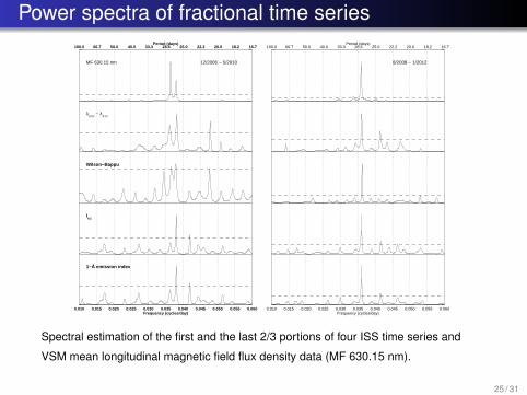
Spectral estimation of the first and the last 2/3 portions of four ISS time series and

VSM mean longitudinal magnetic field flux density data (MF 630.15 nm).

25 / 31

Results from the spectral analysis

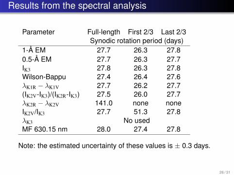
Parameter Full-length First 2/3 Last 2/3Synodic rotation period (days)

1-Å EM 27.7 26.3 27.80.5-Å EM 27.7 26.3 27.7IK3 27.8 26.3 27.8Wilson-Bappu 27.4 26.4 27.6λK1R − λK1V 27.7 26.2 27.7(IK2V-IK3)/(IK2R-IK3) 27.5 26.0 27.7λK2R − λK2V 141.0 none noneIK2V/IK3 27.7 51.3 27.8λK3 No usedMF 630.15 nm 28.0 27.4 27.8

Note: the estimated uncertainty of these values is ± 0.3 days.

26 / 31

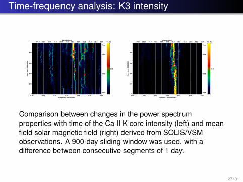
Time-frequency analysis: K3 intensity

99.9

CL (%)

0.00 0.01 0.02 0.03 0.04 0.05 0.06Frequency (cycles/day)

0

200

400

600

800

Day

s si

nce

2/1

2/20

06

200.0 100.0 66.7 50.0 40.0 33.3 28.6 25.0 22.2 20.0 18.2 16.7Period (days)

2007

2008

2009

Year

99.9

CL (%)

0.00 0.01 0.02 0.03 0.04 0.05 0.06Frequency (cycles/day)

0

200

400

600

800

Day

s si

nce

2/1

2/20

06

200.0 100.0 66.7 50.0 40.0 33.3 28.6 25.0 22.2 20.0 18.2 16.7Period (days)

2007

2008

2009

Year

Comparison between changes in the power spectrumproperties with time of the Ca II K core intensity (left) and meanfield solar magnetic field (right) derived from SOLIS/VSMobservations. A 900-day sliding window was used, with adifference between consecutive segments of 1 day.

27 / 31

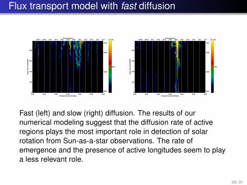
Flux transport model with fast diffusion

99.9

CL (%)

0.00 0.01 0.02 0.03 0.04 0.05 0.06Frequency (cycles/day)

0

200

400

600

800

Day

s si

nce

2/1

2/20

06

200.0 100.0 66.7 50.0 40.0 33.3 28.6 25.0 22.2 20.0 18.2 16.7Period (days)

2007

2008

2009

Year

99.9

CL (%)

0.00 0.01 0.02 0.03 0.04 0.05 0.06Frequency (cycles/day)

0

200

400

600

800

Day

s si

nce

2/1

2/20

06

200.0 100.0 66.7 50.0 40.0 33.3 28.6 25.0 22.2 20.0 18.2 16.7Period (days)

2007

2008

2009

Year

Fast (left) and slow (right) diffusion. The results of ournumerical modeling suggest that the diffusion rate of activeregions plays the most important role in detection of solarrotation from Sun-as-a-star observations. The rate ofemergence and the presence of active longitudes seem to playa less relevant role.

28 / 31

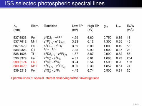
ISS selected photospheric spectral lines

λ0 Elem. Transition Low EP High EP geff Icore EQW(nm) (eV) (eV) (mÅ)

537.6833 Fe I b1D22 - v3P◦1 4.29 6.60 0.750 0.85 13

537.7612 Mn I z4P◦5/2- e4S3/2 3.83 6.12 1.300 0.65 45

537.9579 Fe I b1G24 - z1H◦5 3.69 6.00 1.000 0.49 56

538.0323 C I 1P◦1 - 1P1 7.68 9.99 1.000 0.87 26

538.1026 Ti II b2D23/2 - z2F◦5/2 1.57 3.87 0.900 0.52 56

538.3379 Fe I z5G◦5 - e5H6 4.31 6.61 1.083 0.23 204

539.3174 Fe I z5D◦3 - e5D4 3.24 5.54 1.500 0.26 153

539.4672 Mn I a6S5/2 - z8P◦7/2 0.00 2.30 1.857 0.51 74

539.5218 Fe I z5G◦2 - g5F1 4.45 6.74 0.500 0.81 20

Spectral lines of special interest deserving further investigations

29 / 31

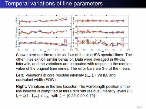
Temporal variations of line parameters

30 / 31

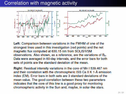
Correlation with magnetic activity

31 / 31