The concept of electoral competition plays a central role

econstorMake Your Publications Visible.

A Service of

zbwLeibniz-InformationszentrumWirtschaftLeibniz Information Centrefor Economics

Cox, Gary W.; Fiva, Jon H.; Smith, Daniel M.

Working Paper

Measuring the Competitiveness of Elections

CESifo Working Paper, No. 7418

Provided in Cooperation with:Ifo Institute – Leibniz Institute for Economic Research at the University of Munich

Suggested Citation: Cox, Gary W.; Fiva, Jon H.; Smith, Daniel M. (2018) : Measuring theCompetitiveness of Elections, CESifo Working Paper, No. 7418, Center for Economic Studiesand ifo Institute (CESifo), Munich

This Version is available at:http://hdl.handle.net/10419/198778

Standard-Nutzungsbedingungen:

Die Dokumente auf EconStor dürfen zu eigenen wissenschaftlichenZwecken und zum Privatgebrauch gespeichert und kopiert werden.

Sie dürfen die Dokumente nicht für öffentliche oder kommerzielleZwecke vervielfältigen, öffentlich ausstellen, öffentlich zugänglichmachen, vertreiben oder anderweitig nutzen.

Sofern die Verfasser die Dokumente unter Open-Content-Lizenzen(insbesondere CC-Lizenzen) zur Verfügung gestellt haben sollten,gelten abweichend von diesen Nutzungsbedingungen die in der dortgenannten Lizenz gewährten Nutzungsrechte.

Terms of use:

Documents in EconStor may be saved and copied for yourpersonal and scholarly purposes.

You are not to copy documents for public or commercialpurposes, to exhibit the documents publicly, to make thempublicly available on the internet, or to distribute or otherwiseuse the documents in public.

If the documents have been made available under an OpenContent Licence (especially Creative Commons Licences), youmay exercise further usage rights as specified in the indicatedlicence.

www.econstor.eu

7418 2018 December 2018

Measuring the Competitive-ness of Elections Gary W. Cox, Jon H. Fiva, Daniel M. Smith

Impressum:

CESifo Working Papers ISSN 2364‐1428 (electronic version) Publisher and distributor: Munich Society for the Promotion of Economic Research ‐ CESifo GmbH The international platform of Ludwigs‐Maximilians University’s Center for Economic Studies and the ifo Institute Poschingerstr. 5, 81679 Munich, Germany Telephone +49 (0)89 2180‐2740, Telefax +49 (0)89 2180‐17845, email [email protected] Editors: Clemens Fuest, Oliver Falck, Jasmin Gröschl www.cesifo‐group.org/wp An electronic version of the paper may be downloaded ∙ from the SSRN website: www.SSRN.com ∙ from the RePEc website: www.RePEc.org ∙ from the CESifo website: www.CESifo‐group.org/wp

CESifo Working Paper No. 7418 Category 2: Public Choice

Measuring the Competitiveness of Elections

Abstract The concept of electoral competition plays a central role in many subfields of political science, but no consensus exists on how to measure it. One key challenge is how to conceptualize and measure electoral competitiveness at the district level across alternative electoral systems. Recent efforts to meet this challenge have introduced general measures of competitiveness which rest on explicit calculations about how votes translate into seats, but also implicit assumptions about how effort maps into votes (and how costly effort is). We investigate how assumptions about the effort-to-votes mapping affect the units in which competitiveness is best measured, arguing in favor of vote-share denominated measures and against vote-share-per-seat measures. Whether elections under multimember proportional representation systems are judged more or less competitive than single-member plurality or runoff elections depends directly on the units in which competitiveness is assessed (and hence on assumptions about how effort maps into votes).

JEL-Codes: D720.

Keywords: competitiveness, measurement, electoral systems, mobilization, turnout.

Gary W. Cox Department of Political Science

Stanford University 100 Encina Hall West, 616 Serra St.

USA – Stanford, CA 94305 [email protected]

Jon H. Fiva Department of Economics

BI Norwegian Business School Norway – 0442 Oslo

[email protected]

Daniel M. Smith

Department of Government Harvard University

1737 Cambridge Street USA – Cambridge, MA 02138

[email protected]

December 12, 2018 We thank Georgina Evans for research assistance, Olle Folke, Torben Iversen, and Janne Tukiainen for comments, and Peter Selb for kindly sharing his replication data and codes.

The concept of electoral competition plays a central role in many subfields of political

science. Political theorists often define democracy as a system in which at least two

parties compete in elections for the right to govern (e.g., Schumpeter, 1942; Downs, 1957;

Dahl, 1971). In other words: no competition, no democracy. Beyond the simple question

of whether elections are contested, however, great interest also surrounds the question

of how closely those elections are contested. Those who investigate the incumbency

advantage, for example, often worry that it reduces the competitiveness of elections due

to the deterrence of high-quality challengers (e.g., Carson, Engstrom and Roberts, 2007;

Hall and Snyder, 2015). Others have argued that uncompetitive elections make for less

responsive politicians (e.g., Fiorina, 1973; Griffin, 2006), and numerous others still have

focused on the relationship between competitiveness and voter turnout (e.g., Riker and

Ordeshook, 1968; Cox, 2015).

Given the ubiquity of references to competition and competitiveness, it is surprising

that no consensus exists on how best to measure it. A key challenge is how to conceptu-

alize and measure electoral competitiveness across alternative electoral systems. Studies

of single-member district (SMD) elections have repeatedly investigated how “safe” and

“swing” districts affect the nature of local politics—in terms of the parties’ mobiliza-

tional efforts, campaign expenditures, and turnout (e.g., Denver and Hands, 1974; Cox

and Munger, 1989; Aldrich, 1993).1 The “traditional” measure of competitiveness in

SMDs used in these studies is based on the simple difference in vote shares between the

winner and the runner-up. Much less consensus exists on how to measure competitiveness

in multi-member district (MMD) contexts, especially under proportional representation

(PR) rules. Elections under PR rules typically involve multiple parties and hence greater

complexity in the nature of competition.

1One issue, which we do not consider here, is whether ex ante competitiveness can be inferred from expost measures of actual vote margins (e.g., Cox, 1988). We also do not consider variations in proportionalsystems, such as options for preference voting or vote transfers, and we assume the D’Hondt allocationmethod in our theoretical and empirical investigations. Finally, while the theoretical logic that we presentassumes that mobilizational effort will increase with competitiveness, it is also possible that decisions byparties or candidates to mobilize voters may also in turn increase competitiveness. We do not attemptto parse the directionality or mutually reinforcing nature of these effects here.

1

A small number of recent studies have attempted to create general measures of com-

petitiveness that can be applied across SMD and MMD systems. Some focus on the

aggregate level, assessing the governing party’s probability of losing office (Kayser and

Lindstadt, 2015; Abou-Chadi and Orlowski, 2016) or how far a party is from winning a

majority in a legislative chamber (Feigenbaum, Fouirnaies and Hall, 2017).2 A second

approach focuses on the closeness of individual candidates to being elected (e.g., Kotako-

rpi, Poutvaara and Tervio, 2017), with the empirical aim of investigating candidate-level

outcomes.

A third set of studies has focused on how to measure competitiveness at the district

level. Three recent papers in particular—Blais and Lago (2009), Grofman and Selb

(2009), and Folke (2014)—have proposed general measures of competitiveness that can

be applied to districts of varying magnitude across alternative electoral systems.3 The

authors use their proposed measures to investigate whether PR induces more competitive

contests than plurality rule (Blais and Lago, 2009; Grofman and Selb, 2009), to predict

turnout across districts in PR systems (Blais and Lago, 2009; Grofman and Selb, 2011),

and to explore the policy influence of small parties in PR systems (Folke, 2014).

In what follows, we offer a reconsideration of how to measure the competitiveness of

elections at the district level in SMD and MMD contexts. We first review the extant

alternative measures and situate them within a typology of possible measures. Next, we

argue that any measure of competitiveness should reflect the marginal benefit of effort

(MBE) for each party. A party’s MBE depends on how its effort maps into votes, how

votes map into seats, and how valuable seats are. While all three recently proposed

measures rest on explicit calculations about how votes translate into seats, each relies on

implicit assumptions about how effort maps into votes (and how costly effort is). Whether

PR contests in MMDs are judged more or less competitive than single-member plurality

2Even simpler aggregate measures use 100 minus the largest party’s vote share to capture “competi-tion,” with obvious limitations (e.g., Gerring et al., 2015). Other approaches focus on aggregate volatilityin electoral behavior (i.e., party-switching) at the voter level (e.g., Wagner, 2017).

3Collectively, these studies—which define the state of the art—have garnered more than 250 citations,according to Google Scholar (as of December, 2018).

2

(SMP) or majority runoff contests in SMDs depends directly on such assumptions.

Blais and Lago (2009) and Grofman and Selb (2009) show that different measures

of competitiveness give different answers to questions about the level and variability

of competition in PR systems with MMDs. We reproduce this finding using district-

level data from Norway (1909-1927) and Switzerland (1971-2003). The Swiss case has

previously been featured by Grofman and Selb (2009), and is useful due to within-country

variation in district magnitude, including SMDs as well as MMDs. The Norwegian case

we introduce to the body of empirical evidence offers an additionally useful context of

within-country variation, as an electoral reform in 1919 shifted all elections from SMD to

MMD contests with varying magnitude (see Cox, Fiva and Smith, 2019). We argue that

the determination of whether elections in MMD systems are more or less competitive than

SMD systems stems primarily from the different units in which distances are expressed

by different measures. In particular, it matters a lot whether distances are denominated

in vote shares (the traditional measure) or vote shares per seat (revisionist measures).

On the basis of our theoretical logic, and survey data from both countries capturing the

modes through which parties mobilize voters under alternative electoral rules, we argue

that the vote-share-denominated measure of distance makes more sense.

Finally, we investigate the construct validity of the different measures of competitive-

ness. If a particular measure accurately reflects how close local elites perceive a given

electoral contest to be, then it should be useful in predicting their mobilizational ef-

forts and, hence, turnout. Using again the district-level data from Norwegian and Swiss

elections covering both SMD and MMD elections, we contrast two families of distance

measure—those denominating distances in vote shares (the traditional measure) and those

denominating distances in vote shares per seat (those of Blais-Lago or Grofman-Selb).

As do Blais-Lago and Grofman-Selb, we show that the relationship between distance

and turnout attenuates as district magnitude increases (regardless of the distance met-

ric used). While we agree with Blais-Lago and Grofman-Selb regarding the pattern of

evidence, this pattern directly impugns the construct validity of vote-share-per-seat mea-

3

sures but can easily be accommodated by vote-share measures. Accordingly, we argue in

favor of vote-share measures as the most appropriate generalized measure of district-level

competitiveness across different electoral systems.

Measuring the competitiveness of district elections

For SMD contests, the traditional measure of competitiveness is the simple difference in

observed vote shares between the winner of the seat and the runner-up—expressed as

a vote share, rather than in raw votes. This measure makes intuitive sense for SMD

contests, but measuring competitiveness in MMD contests requires more consideration.

Suppose J parties are competing in a given electoral district in which M ≥ 1 seats will

be awarded, and all M seats will be allocated based on the votes cast in the district (no

upper tiers). Moreover, neither joint lists nor apparentements are allowed. How should

one measure the competitiveness of the contest between the J parties?

Let Vj denote the number of votes received by party j, for j = 1, ..., J . Let V• ≡∑Jj=1 Vj be the total votes cast, and vj = Vj/V• be j’s share of the votes. For a given

vote vector V = (V1, ..., VJ), the seat vector S(V ) = (S1(V ), ..., SJ(V )) gives the number

of seats awarded to each party. The mapping V → S(V ) is determined by the electoral

rules in force.

Now consider how many votes would have to change, in order to change the seat

allocation.4 To answer this question, one needs a metric of the “distance” to a seat

change.

4Freier and Odendahl (2015) take a different approach for measuring electoral closeness. The basicidea of their method is to simulate the voting result of a given election repeatedly, adding noise to theelection result. In some of those simulated election results, the seat allocation will be different. If thathappens often, they consider the seat allocation as close. Kotakorpi, Poutvaara and Tervio (2017) takea similar simulation-based approach.

4

Single-party versus multi-party measures

The single-party measure upon which we shall initially focus begins by calculating two

numbers. First, N+j (V ) is the minimum number of votes that j must gain in order to

win an additional seat, holding the other parties’ votes constant.5 Second, N−j (V ) is

the minimum number of votes that j must lose in order to lose a seat, holding the other

parties’ votes constant.6

The smaller of the raw vote counts, Nj(V ) = min{N+j (V ), N−j (V )}, is taken as

measuring j’s incentive to mobilize, given the vote vector V . We shall henceforth simplify

our notation, writing just N+j , N−j , and Nj, the dependence on V being understood. We

will consider how to normalize or scale Nj later.

Any single-party measure must make assumptions about the other parties when it cal-

culates the minimum votes a given party would need to gain in order to win an additional

seat. Grofman and Selb (2009) focus on a worst-case scenario for the focal party: What

is the minimum increase in votes that would guarantee the party another seat (regardless

of vote reallocations among the other parties)?7 Let NGS+j denote the answer. Blais and

Lago (2009), in contrast, consider the scenario in which all other parties’ votes are held

constant. In other words, they focus on N+j .

Rather than considering hypothetical vote gains (or losses) by a single party, one might

instead consider patterns of gains and losses across all the parties. Let R = (R1, ..., RJ)

be a vector of raw vote gains (Rj > 0) or losses (Rj < 0). Let R(j)• be the “smallest”

change that gives an additional seat to party j. That is, R(j)• =

∑Jh=1|R

(j)h |. In other

5Formally, N+j (V ) can be defined implicitly by the following equations: Sj(Vj ,V−j) = Sj [(Vj +

N+j (V )− 1,V−j)] = Sj [(Vj + N+

j (V ),V−j ]− 1. We assume that ties are always broken unfavorably forthe focal party. The formulas would become somewhat more complex if ties were broken by coin flips.

6In other words, N−j (V ) is such that Sj(Vj ,V−j) = Sj [(Vj − N−j (V ) + 1,V−j)] = Sj [(Vj −N−j (V ),V−j)] + 1.

7More specifically, Grofman and Selb (2009) begin by identifying two values representing “worst-casescenarios” for each party, indexed by i: the vote share required to gain an additional seat, XG

i , and thevote share required to lose a seat, XL

i . They then take the larger of the two resulting values when eachis subtracted from the threshold of exclusion, TE (for D’Hondt, 1/(M + 1)), and then also divide thisnumber by the threshold of exclusion. The resultant party-specific measure, ci, using their notation is

thus: ci =max[(TE−XG

i ),(TE−XLi )]

TE .

5

words, R(j)• represents the smallest number of votes that would have to be added or

subtracted, without restricting which party was gaining or losing the votes, in order to

confer an additional seat on party j. This is the distance metric proposed by Folke (2014),

measured in the form of vote shares. Note that the votes that a particular party gains

can be generated either by mobilizing supporters who were previously not voting or by

persuading other parties’ supporters to change their votes.

Issues of aggregation and units

Any measure of the distance in votes to a seat change must answer the following two

questions. First, how should the party-specific distances be aggregated into a district-

wide measure? One approach would be to focus on the single party with the strongest

incentive to mobilize. Blais and Lago (2009, p. 96) take this approach, calculating “the

minimal number of additional votes required, under the existing rules, for any party to

win one additional seat.”8 Grofman and Selb (2009) instead opt for a weighted average,

where the weights are the parties’ respective vote shares.9 In our empirical analysis, we

consider aggregations of both types—minima and weighted averages—finding that there

is not much difference in the resulting measures.

Second, in what units should the vote distances be expressed? Should distances be

stated in raw votes? Should they be stated in shares of the vote (as in the traditional

measure for SMDs, and in Folke’s measure for MMDs)? Or, should they be expressed as

shares of the votes cast per seat (following Blais and Lago, 2009, and Grofman and Selb,

2009)?10 We discuss this issue further in the next section.

8More specifically, the Blais-Lago measure, BL, takes this raw number of votes, divides it by the rawnumber of total votes cast per seat (i.e., total votes in the district divided by M), and then multipliesthis fraction by 100: BL = 100 ∗ votes needed to win one additional seat

number of ballots per seat .9The authors take the sum of ci (discussed in footnote 7) for all parties weighted by each party’s vote

share, vi, and define this district-level “index of competition” as C =n∑

i=1

vi ∗ ci.10Actually, Grofman and Selb normalize by the threshold of exclusion ( 1

M+1 ), while Blais and Lago

normalize by 1M , where M is district magnitude. This difference does not matter for our discussions.

6

The marginal benefit of effort

If vote distances reflect parties’ perceptions of electoral competitiveness, then they should

be able to predict how parties exert campaign effort. In this section, we imagine that

each party j can exert some kind of mobilizational effort, denoted by ej. For example,

ej might represent the number of advertisements (urging supporters to vote) that party

j purchases. Let e = (e1, ..., eJ) represent the choices made by all parties.

Let the parties’ expected vote shares, given e, be denoted v(e) = (v1(e), ..., vJ(e))

and their expected seat shares, given v, be denoted s(v) = (s1(v), ..., sJ(v)). We continue

to use lower-case variables for vote or seat shares, reserving upper-case variables for raw

totals. The mapping v → s(v) depends on the electoral rules.

We shall assume that party j’s payoff equals sj(v(e))Mb−c(ej). The first term reflects

j’s expected share sj(v(e)) of the M seats at stake in the district, each of which is worth

b utils.11 Against this expected benefit must be weighed the cost of effort, denoted by

c(ej).

The marginal benefit of effort for party j (MBEj) can be written as follows:

MBEj ≡∂sj(v(e))Mb

∂ej=

∂vj∂ej

∂sj∂vj

Mb (1)

Equation (1) reveals that party j’s MBE depends on three factors: how quickly effort

translates into votes (∂vj∂ej

); how quickly votes translate into seats (∂sj∂vj

); and the total

value of the seats at stake (Mb). The larger the MBE is, the greater the party’s incentive

to mobilize its supporters and, thus, the higher turnout is expected to be (Cox, 1999;

Herrera, Morelli and Palfrey, 2014).

Extant measures of competitiveness focus exclusively on the votes-to-seats mapping.

Their respective authors offer various ways of calculating the minimum votes needed

11We do not assume that a seat in one country is of equal value to a seat in another, only that all seatsin any given country (at a given time) are equally valuable. This assumption simplifies our theoreticalargument, but it is nevertheless plausible that winning the majority-achieving seat, say, might be morevaluable than winning any other seat in multiparty systems (Freier and Odendahl, 2015).

7

to change the seat allocation in j’s favor. These minimum vote measures—e.g., NGS+j ,

N+j , R

(j)• —suggest “how fast” more votes will turn into additional seats. They, or more

precisely their normalized inverses, can thus proxy for∂sj∂vj

in Equation (1).

The importance of the effort-to-votes mapping

If∂vj∂ej

= 0, then it does not matter how large or small the vote distance to a seat change is.

Thus, if they are to be useful in predicting parties’ mobilizational efforts, extant measures

must rely on some assumptions about how effort translates into votes.

To further explain this observation, consider a hypothetical area in which two parties,

A and B, compete. Each party’s supporters are uniformly distributed across the area.

The area can be carved into electoral districts in various ways—all single-seat districts,

a mix of 1-seat and 2-seat districts, and so forth. We assume perfect apportionment:

a single-seat district has n voters, a 2-seat district has 2n voters, and so on. We also

assume that the seats in each district are allocated by the D’Hondt rule.

Suppose that in each district in the area, in the absence of any mobilization, party A

is expected to get all the votes and party B none. This scenario—the least competitive

possible—makes it easy to compute the minimum votes needed to change the seat alloca-

tion. (The reason party B expects to get zero votes, let us say, is that all of its supporters

bear positive costs of participation while some of party A’s supporters have non-positive

costs; thus, there is a Nash equilibrium in which none of party B’s supporters vote and

some of party A’s supporters do.)

Figure 1 plots the distance to a seat gain for party B denominated in vote shares

(top-left panel) and raw votes (top-right panel) against district magnitude. While the

share of votes party B needs to gain a seat falls with district magnitude, the opposite

is true for raw votes (in the example, n=1,000).12 Instead of focusing on the number

or share of votes that party B needs to gain its first seat, consider the minimum effort

12The top-left panel of Figure 1 is essentially plotting the threshold of exclusion, defined as the max-imum share that a party can possibly win while still failing to win a seat, against district magnitudeunder the D’Hondt allocation rule.

8

0.1

.2.3

.4.5

Vote

sha

re

1 2 3 4 5 6 7 8 9 10 11 12 13 14 15M

(i) Share of votes B needs to gain a seat

025

050

075

010

00Vo

tes

1 2 3 4 5 6 7 8 9 10 11 12 13 14 15M

(ii) Raw votes B needs to gain a seat

12

34

5Ad

s

1 2 3 4 5 6 7 8 9 10 11 12 13 14 15M

(iii) Ads B needs to run in order to gain a seat

050

010

0015

0020

00C

onta

cts

1 2 3 4 5 6 7 8 9 10 11 12 13 14 15M

(iv) Contacts B needs to make to gain a seat

Figure 1: Effort, votes, and seats: which units should be used for measurement?Note: We consider a situation where two parties, A and B, compete for office in a PR system with districts of varying

magnitude (M), where, in the absence of mobilization, party A is expected to get all the votes. This figure illustrates

the relationship between district magnitude and (i) the share of votes party B needs to gain a seat (i.e., the threshold of

exclusion), (ii) the number of votes B needs to gain a seat, (iii) the number of ads B needs to run, to gain a seat, and

(iv) the individual contacts B needs to make, to gain a seat. We assume that seats are allocated by the D’Hondt rule, the

number of eligible voters is 1000 ·M (perfect apportionment), each ad mobilizes 10 percent of voters (z = 0.1), and that

every other individual contacted is persuaded to vote (y = 0.5). Appendix Table A.1 summarizes the distances to a seat

gain for party B in table format.

9

it would have to exert, in order to gain its first seat. Does that effort increase with M ,

because the technology of mobilization exhibits no economies of scale? Or does it decline,

because there are economies of scale in mobilization?

An example of a scalable mobilization technology is advertising in a mass media

market that covers the area. Suppose a unit ad mobilizes the same positive proportion

of voters, z > 0, regardless of where they reside in the market; and that ads translate

linearly into vote shares: each additional ad generates the same increase in vote share (at

least over some range). Thus, if an ad is purchased and the election in question is held

in a 1-seat district, then the ad yields nz votes. If the election in question is held in a

2-seat district, then the ad yields 2nz votes. And so on.

The effort distance—the minimum number of ads a party must run to gain an addi-

tional seat—is dads(z,M) = 1(M+1)z

. Note that the effort distance declines with district

magnitude: ∂dads(z,M)/∂M < 0. We illustrate this result in the bottom-left panel of

Figure 1 where we assume z = 0.1. If the cost of running ads is a concave increasing

function of ej(c′ > 0, c′′ ≤ 0), then the cost distance—the minimum cost a party must

bear to gain an additional seat—is also declining in M .

Now suppose that mobilization consists of contacting individual voters and persuad-

ing them to vote—which might entail bribes or non-monetary encouragement delivered

through “get out the vote” drives or door-to-door canvassing.13 In this case, the effort

distance—the number of contacts a party needs to make to gain an additional seat—is

dcon(y, n,M) = Mn(M+1)y

, where y is the probability that a contact succeeds in mobilizing

the voter (who then votes for the mobilizing party). Thus, the effort distance increases

with district magnitude: ∂dcon(y, n,M)/∂M > 0. We illustrate this result in the bottom-

right panel of Figure 1, where we assume a (constant) success rate of 0.5. Given convex

increasing costs of contacting (c′ > 0, c′′ ≥ 0), the cost distance is also increasing in M .14

These observations lead to our first general conclusion. Parties’ decisions to mobilize

13For simplicity, in what follows we assume no spillovers from personal contacts. See Cox (2015) for aconsideration of models in which spillovers occur.

14Convex increasing costs here might also arise because it becomes increasingly difficult to mobilizethose contacted, as the number previously contacted increases.

10

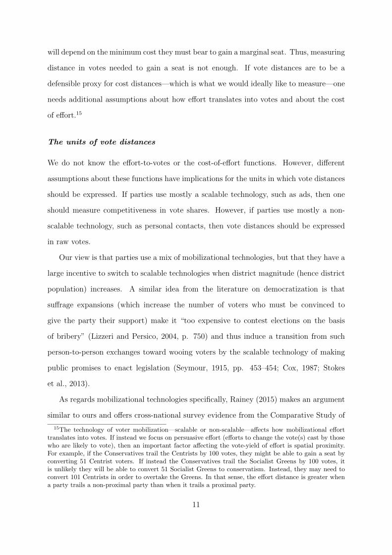
will depend on the minimum cost they must bear to gain a marginal seat. Thus, measuring

distance in votes needed to gain a seat is not enough. If vote distances are to be a

defensible proxy for cost distances—which is what we would ideally like to measure—one

needs additional assumptions about how effort translates into votes and about the cost

of effort.15

The units of vote distances

We do not know the effort-to-votes or the cost-of-effort functions. However, different

assumptions about these functions have implications for the units in which vote distances

should be expressed. If parties use mostly a scalable technology, such as ads, then one

should measure competitiveness in vote shares. However, if parties use mostly a non-

scalable technology, such as personal contacts, then vote distances should be expressed

in raw votes.

Our view is that parties use a mix of mobilizational technologies, but that they have a

large incentive to switch to scalable technologies when district magnitude (hence district

population) increases. A similar idea from the literature on democratization is that

suffrage expansions (which increase the number of voters who must be convinced to

give the party their support) make it “too expensive to contest elections on the basis

of bribery” (Lizzeri and Persico, 2004, p. 750) and thus induce a transition from such

person-to-person exchanges toward wooing voters by the scalable technology of making

public promises to enact legislation (Seymour, 1915, pp. 453–454; Cox, 1987; Stokes

et al., 2013).

As regards mobilizational technologies specifically, Rainey (2015) makes an argument

similar to ours and offers cross-national survey evidence from the Comparative Study of

15The technology of voter mobilization—scalable or non-scalable—affects how mobilizational efforttranslates into votes. If instead we focus on persuasive effort (efforts to change the vote(s) cast by thosewho are likely to vote), then an important factor affecting the vote-yield of effort is spatial proximity.For example, if the Conservatives trail the Centrists by 100 votes, they might be able to gain a seat byconverting 51 Centrist voters. If instead the Conservatives trail the Socialist Greens by 100 votes, itis unlikely they will be able to convert 51 Socialist Greens to conservatism. Instead, they may need toconvert 101 Centrists in order to overtake the Greens. In that sense, the effort distance is greater whena party trails a non-proximal party than when it trails a proximal party.

11

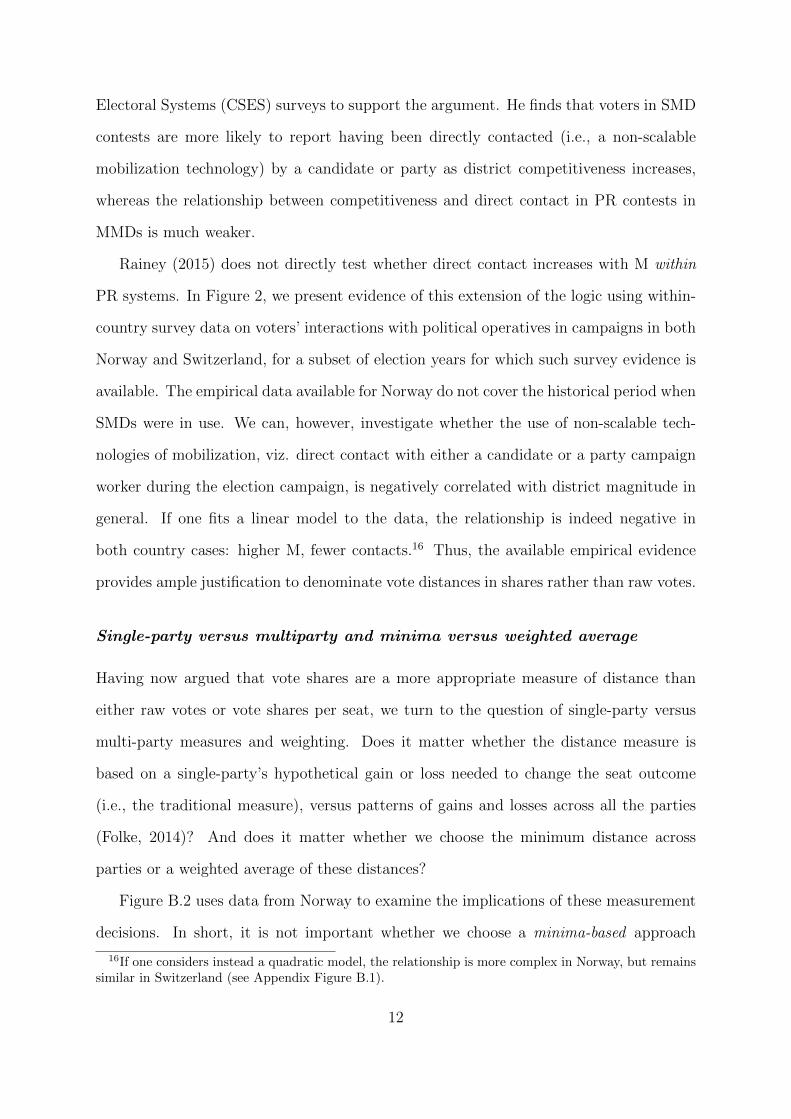
Electoral Systems (CSES) surveys to support the argument. He finds that voters in SMD

contests are more likely to report having been directly contacted (i.e., a non-scalable

mobilization technology) by a candidate or party as district competitiveness increases,

whereas the relationship between competitiveness and direct contact in PR contests in

MMDs is much weaker.

Rainey (2015) does not directly test whether direct contact increases with M within

PR systems. In Figure 2, we present evidence of this extension of the logic using within-

country survey data on voters’ interactions with political operatives in campaigns in both

Norway and Switzerland, for a subset of election years for which such survey evidence is

available. The empirical data available for Norway do not cover the historical period when

SMDs were in use. We can, however, investigate whether the use of non-scalable tech-

nologies of mobilization, viz. direct contact with either a candidate or a party campaign

worker during the election campaign, is negatively correlated with district magnitude in

general. If one fits a linear model to the data, the relationship is indeed negative in

both country cases: higher M, fewer contacts.16 Thus, the available empirical evidence

provides ample justification to denominate vote distances in shares rather than raw votes.

Single-party versus multiparty and minima versus weighted average

Having now argued that vote shares are a more appropriate measure of distance than

either raw votes or vote shares per seat, we turn to the question of single-party versus

multi-party measures and weighting. Does it matter whether the distance measure is

based on a single-party’s hypothetical gain or loss needed to change the seat outcome

(i.e., the traditional measure), versus patterns of gains and losses across all the parties

(Folke, 2014)? And does it matter whether we choose the minimum distance across

parties or a weighted average of these distances?

Figure B.2 uses data from Norway to examine the implications of these measurement

decisions. In short, it is not important whether we choose a minima-based approach

16If one considers instead a quadratic model, the relationship is more complex in Norway, but remainssimilar in Switzerland (see Appendix Figure B.1).

12

0.0

5.1

.15

.2Vi

sit b

y ca

mpa

ign

wor

ker

4 6 8 10 12 14M

Norway

0.0

5.1

.15

.2C

onve

rsat

ion

with

can

dida

te

1 5 10 15 20 25 30 35M

Switzerland

Figure 2: Direct contact and district magnitude: survey evidence of the use ofnon-scalable mobilization technologyNote: The figure shows the relationship between a non-scalable mobilization technology—direct contact by campaign

workers and candidates—and district magnitude. The left-hand panel uses data from the 1965-1969 Norwegian Election

Studies surveys (N=3,099) made available by Norwegian Center for Research Data (NSD). Respondents were asked whether

any party’s campaign worker visited them during the campaign. The right-hand panel uses data from the 1987-1991 Swiss

National Election Studies surveys (N=1,895) made available by the Swiss Centre of Expertise in the Social Sciences

(FORS). Respondents were asked if they made use of conversations with candidates as information regarding the election

campaign. In each panel, we show binned scatterplots residualized by year fixed effects and survey respondent background

characteristics (age, gender, education level, and marital status). Appendix Figure B.1 presents the data with a quadratic

fit line.

13

rather than a weighted-average approach. The correlation between the two alternative

measures is 0.95 in our sample. Nor is it important whether we take a single-party rather

than a multi-party approach. For simplicity, we use the single-party minima measure in

the remainder of our investigations.

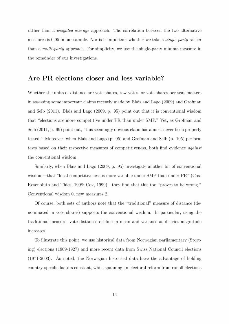
Are PR elections closer and less variable?

Whether the units of distance are vote shares, raw votes, or vote shares per seat matters

in assessing some important claims recently made by Blais and Lago (2009) and Grofman

and Selb (2011). Blais and Lago (2009, p. 95) point out that it is conventional wisdom

that “elections are more competitive under PR than under SMP.” Yet, as Grofman and

Selb (2011, p. 99) point out, “this seemingly obvious claim has almost never been properly

tested.” Moreover, when Blais and Lago (p. 95) and Grofman and Selb (p. 105) perform

tests based on their respective measures of competitiveness, both find evidence against

the conventional wisdom.

Similarly, when Blais and Lago (2009, p. 95) investigate another bit of conventional

wisdom—that “local competitiveness is more variable under SMP than under PR” (Cox,

Rosenbluth and Thies, 1998; Cox, 1999)—they find that this too “proves to be wrong.”

Conventional wisdom 0, new measures 2.

Of course, both sets of authors note that the “traditional” measure of distance (de-

nominated in vote shares) supports the conventional wisdom. In particular, using the

traditional measure, vote distances decline in mean and variance as district magnitude

increases.

To illustrate this point, we use historical data from Norwegian parliamentary (Stort-

ing) elections (1909-1927) and more recent data from Swiss National Council elections

(1971-2003). As noted, the Norwegian historical data have the advantage of holding

country-specific factors constant, while spanning an electoral reform from runoff elections

14

in SMDs to PR elections in MMDs (Cox, Fiva and Smith, 2016).17 The Swiss data have

the useful feature that district magnitude varies across districts in each election—from

single-seat districts to large multimember districts (Grofman and Selb, 2009).

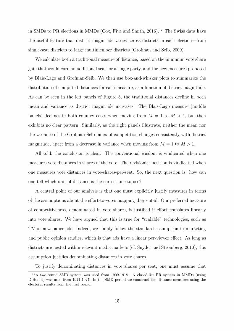
We calculate both a traditional measure of distance, based on the minimum vote share

gain that would earn an additional seat for a single party, and the new measures proposed

by Blais-Lago and Grofman-Selb. We then use box-and-whisker plots to summarize the

distribution of computed distances for each measure, as a function of district magnitude.

As can be seen in the left panels of Figure 3, the traditional distances decline in both

mean and variance as district magnitude increases. The Blais-Lago measure (middle

panels) declines in both country cases when moving from M = 1 to M > 1, but then

exhibits no clear pattern. Similarly, as the right panels illustrate, neither the mean nor

the variance of the Grofman-Selb index of competition changes consistently with district

magnitude, apart from a decrease in variance when moving from M = 1 to M > 1.

All told, the conclusion is clear. The conventional wisdom is vindicated when one

measures vote distances in shares of the vote. The revisionist position is vindicated when

one measures vote distances in vote-shares-per-seat. So, the next question is: how can

one tell which unit of distance is the correct one to use?

A central point of our analysis is that one must explicitly justify measures in terms

of the assumptions about the effort-to-votes mapping they entail. Our preferred measure

of competitiveness, denominated in vote shares, is justified if effort translates linearly

into vote shares. We have argued that this is true for “scalable” technologies, such as

TV or newspaper ads. Indeed, we simply follow the standard assumption in marketing

and public opinion studies, which is that ads have a linear per-viewer effect. As long as

districts are nested within relevant media markets (cf. Snyder and Stromberg, 2010), this

assumption justifies denominating distances in vote shares.

To justify denominating distances in vote shares per seat, one must assume that

17A two-round SMD system was used from 1909-1918. A closed-list PR system in MMDs (usingD’Hondt) was used from 1921-1927. In the SMD period we construct the distance measures using theelectoral results from the first round.

15

0.2

.4.6

.81

Trad

ition

al m

easu

re

1 2 3 4 5 6 7 8M

0.2

.4.6

.81

Blai

s-La

go m

easu

re

1 2 3 4 5 6 7 8M

0.2

.4.6

.81

Gro

fman

-Sel

b m

easu

re

1 2 3 4 5 6 7 8M

Norway

0.2

.4.6

.81

Trad

ition

al m

easu

re

1 2 3 4 5 6 7 8 9 10+M

0.2

.4.6

.81

Blai

s-La

go m

easu

re

1 2 3 4 5 6 7 8 9 10+M

0.2

.4.6

.81

Gro

fman

-Sel

b m

easu

re

1 2 3 4 5 6 7 8 9 10+M

Switzerland

Figure 3: Alternative measures of competitiveness and the relationship of each withdistrict magnitudeNote: The left-hand panels relate the minimum vote share gain that would earn an additional seat for a single party

to district magnitude. The middle panels relate Blais and Lago’s (2009) measure to district magnitude. The right-hand

panels relate Grofman-Selb’s (2009) index of competition to district magnitude. In the top panel, we use the balanced

panel data set of Cox, Fiva and Smith (2016) covering Norway, 1909-1927. Two-round elections were used from 1909-1918,

proportional representation from 1921-1927. In the pre-reform period we construct the distance measures using the electoral

results from the first round. In the bottom panel, we use data from Switzerland, 1971-2003 (Grofman and Selb, 2011). We

exclude one district where voting is compulsory (Schaffhausen).

16

effort translates linearly into vote shares per seat. Thus far, no one has defended such

an assumption; nor do we see an obvious line of argument that could do so. Thus,

purely in terms of grounding each measure in an explicit assumption about the effort-

to-votes mapping, we prefer denominating distances in vote shares, rather than vote

shares per seat. In the next section, we provide an additional reason to prefer vote

share-denominated measures, based on their construct validity.

Construct validity: Does competitiveness predict turnout?

Construct validity is the degree to which inferences can legitimately be made from the

operationalization of a measure to the theoretical construct on which it is based (Trochim

and Donnelly, 2008, p. 56–57). A common method of assessing the construct validity of

a proposed measure is to examine whether it correlates with other variables with which it

should, in theory, correlate. To put it another way, evaluating construct validity involves

examining whether the proposed measure correlates with variables that are known to be

related to the construct.

In our case, the construct of interest is the perceived closeness of an electoral contest.

When elite actors, such as candidates and parties, perceive that a particular district

is more competitive, they should exert more effort to mobilize their supporters, thereby

boosting turnout. These straightforward predictions about mobilization and turnout have

been extensively explored and validated in previous works focusing on SMDs operating

under majoritarian rules (e.g., Denver and Hands, 1974; Cox and Munger, 1989).

What about MMDs operating under PR rules? The Blais-Lago and Grofman-Selb

measures of competitiveness vary considerably across both MMDs in PR systems and

across SMDs in majoritarian systems. Since the operational measure varies widely across

districts in both MMD and SMD systems, elite perceptions should also vary widely—if

the measure has construct validity. Thus, the correlation between district-level competi-

tiveness and turnout should be just as strong in PR systems as in majoritarian systems.

17

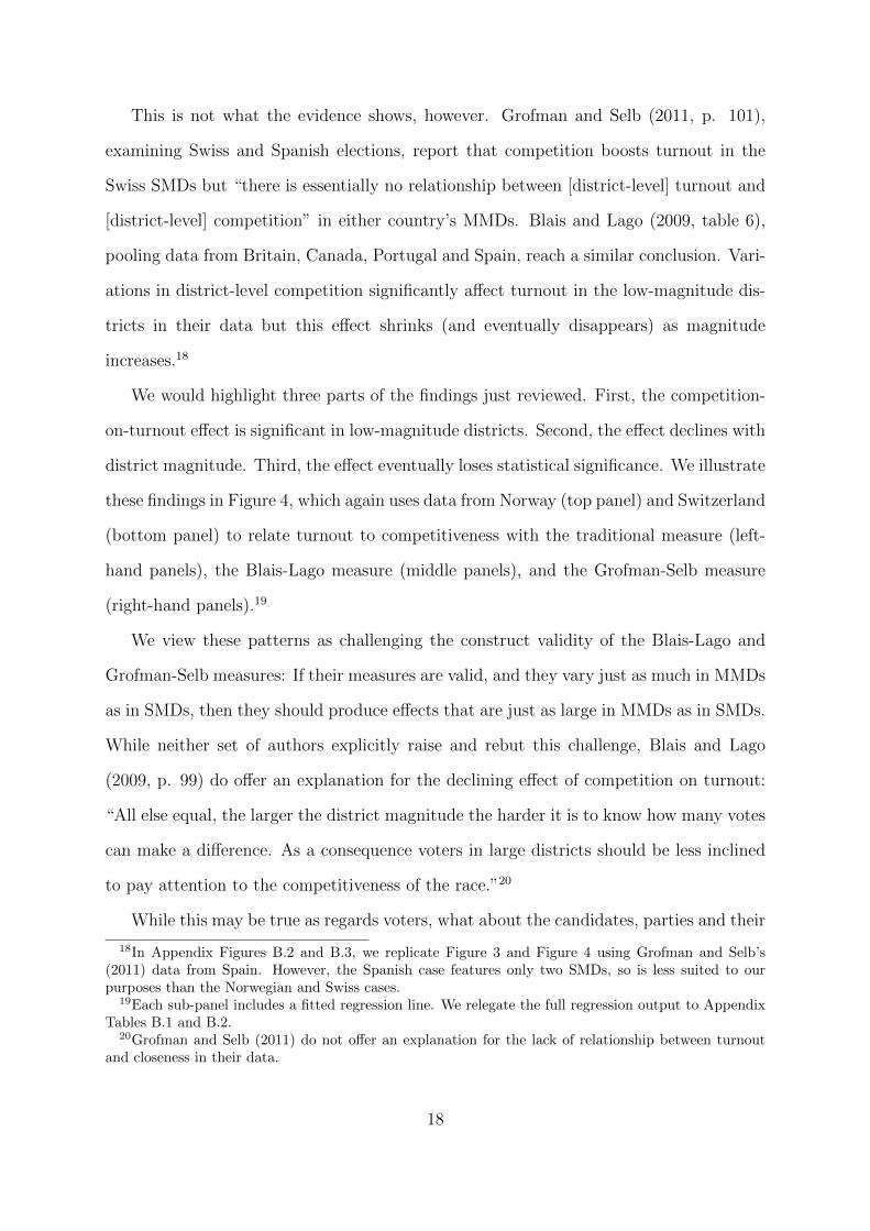
This is not what the evidence shows, however. Grofman and Selb (2011, p. 101),

examining Swiss and Spanish elections, report that competition boosts turnout in the

Swiss SMDs but “there is essentially no relationship between [district-level] turnout and

[district-level] competition” in either country’s MMDs. Blais and Lago (2009, table 6),

pooling data from Britain, Canada, Portugal and Spain, reach a similar conclusion. Vari-

ations in district-level competition significantly affect turnout in the low-magnitude dis-

tricts in their data but this effect shrinks (and eventually disappears) as magnitude

increases.18

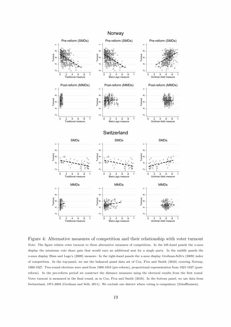
We would highlight three parts of the findings just reviewed. First, the competition-

on-turnout effect is significant in low-magnitude districts. Second, the effect declines with

district magnitude. Third, the effect eventually loses statistical significance. We illustrate

these findings in Figure 4, which again uses data from Norway (top panel) and Switzerland

(bottom panel) to relate turnout to competitiveness with the traditional measure (left-

hand panels), the Blais-Lago measure (middle panels), and the Grofman-Selb measure

(right-hand panels).19

We view these patterns as challenging the construct validity of the Blais-Lago and

Grofman-Selb measures: If their measures are valid, and they vary just as much in MMDs

as in SMDs, then they should produce effects that are just as large in MMDs as in SMDs.

While neither set of authors explicitly raise and rebut this challenge, Blais and Lago

(2009, p. 99) do offer an explanation for the declining effect of competition on turnout:

“All else equal, the larger the district magnitude the harder it is to know how many votes

can make a difference. As a consequence voters in large districts should be less inclined

to pay attention to the competitiveness of the race.”20

While this may be true as regards voters, what about the candidates, parties and their

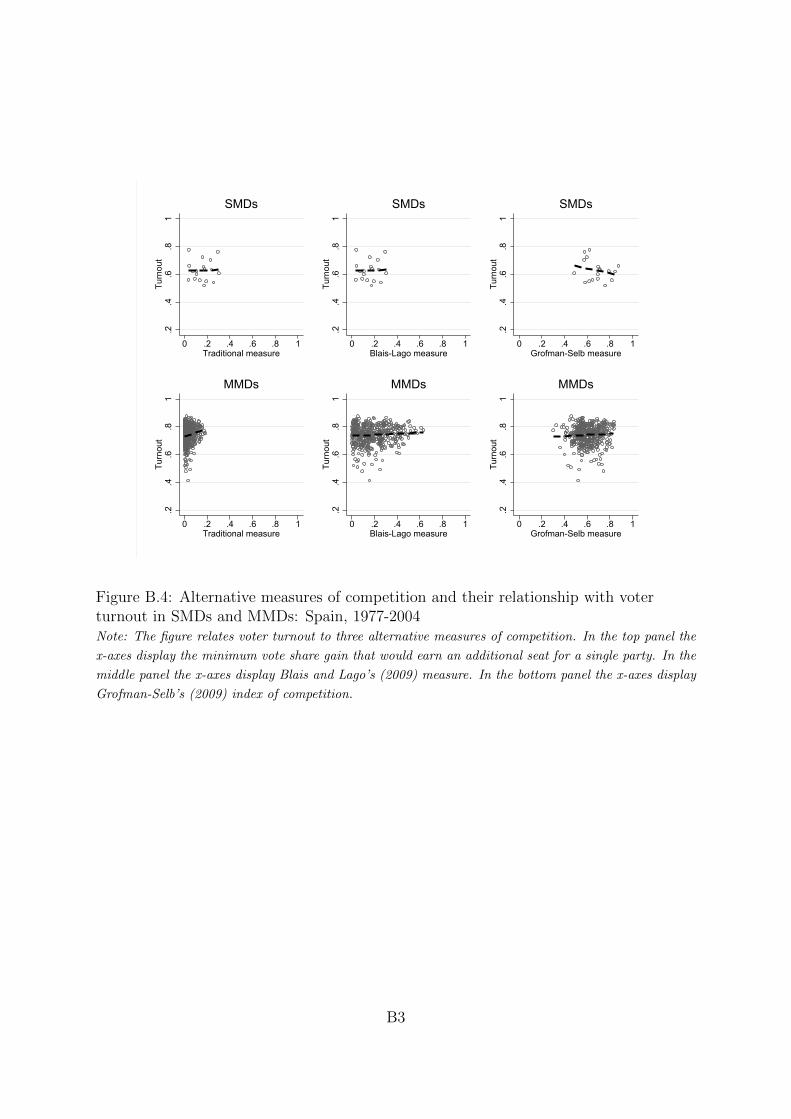
18In Appendix Figures B.2 and B.3, we replicate Figure 3 and Figure 4 using Grofman and Selb’s(2011) data from Spain. However, the Spanish case features only two SMDs, so is less suited to ourpurposes than the Norwegian and Swiss cases.

19Each sub-panel includes a fitted regression line. We relegate the full regression output to AppendixTables B.1 and B.2.

20Grofman and Selb (2011) do not offer an explanation for the lack of relationship between turnoutand closeness in their data.

18

.2.4

.6.8

1Tu

rnou

t

0 .2 .4 .6 .8 1Traditional measure

Pre-reform (SMDs)

.2.4

.6.8

1Tu

rnou

t

0 .2 .4 .6 .8 1Blais-Lago measure

Pre-reform (SMDs)

.2.4

.6.8

1Tu

rnou

t

0 .2 .4 .6 .8 1Grofman-Selb measure

Pre-reform (SMDs)

.2.4

.6.8

1Tu

rnou

t


Post-reform (MMDs)

.2.4

.6.8

1Tu

rnou

t


Post-reform (MMDs)

.2.4

.6.8

1Tu

rnou

t


Post-reform (MMDs)

Norway

.2.4

.6.8

1Tu

rnou

t


SMDs

.2.4

.6.8

1Tu

rnou

t


SMDs.2

.4.6

.81

Turn

out


SMDs

.2.4

.6.8

1Tu

rnou

t


MMDs

.2.4

.6.8

1Tu

rnou

t


MMDs

.2.4

.6.8

1Tu

rnou

t


MMDs

Switzerland

Figure 4: Alternative measures of competition and their relationship with voter turnoutNote: The figure relates voter turnout to three alternative measures of competition. In the left-hand panels the x-axes

display the minimum vote share gain that would earn an additional seat for a single party. In the middle panels the

x-axes display Blais and Lago’s (2009) measure. In the right-hand panels the x-axes display Grofman-Selb’s (2009) index

of competition. In the top-panel, we use the balanced panel data set of Cox, Fiva and Smith (2016) covering Norway,

1909-1927. Two-round elections were used from 1909-1918 (pre-reform), proportional representation from 1921-1927 (post-

reform). In the pre-reform period we construct the distance measures using the electoral results from the first round.

Voter turnout is measured in the final round, as in Cox, Fiva and Smith (2016). In the bottom panel, we use data from

Switzerland, 1971-2003 (Grofman and Selb, 2011). We exclude one district where voting is compulsory (Schaffhausen).

19

in-house pollsters? Suppose we have observations on many SMDs, some of which are “very

competitive” and some of which are “uncompetitive.” We can use these observations to

calibrate what “very competitive” and “uncompetitive” means, in terms of the Blais-Lago

(or Grofman-Selb) distance metric.

Now suppose that a particular 10-seat district varies substantially over time in com-

petitiveness, as measured by Blais-Lago (or Grofman-Selb). The local elites should notice,

even if the local voters do not, that their district is “very competitive” in one year and

“uncompetitive” in another. They should more intensively mobilize their supporters in

the first year than in the second. Turnout should be higher in the first year than the

second. Thus, one cannot explain the disappearance of the competition-on-turnout effect

simply by referring to the voters’ lack of information about how close the contest is in

higher-magnitude districts—because local elites should have good information and the

resources to act on that information.

We offer a different explanation for the disappearance of the competition-on-turnout

effect. As noted in the previous section, the distribution of vote-share distances changes

dramatically as district magnitude increases: both the mean and variance shrink toward

zero. Thus, there are two reasons to expect that the competition-on-turnout effect should

disappear. The first is substantive: in high-magnitude districts, competitiveness will have

a high mean and low variance, so elites’ mobilizational effort will also have a high mean

and low variance. The second reason is statistical: attenuation bias. If the range over

which an independent variable is observed shrinks toward zero, the estimated impact of

that variable on any dependent variable will also shrink toward zero (as long as there is

some measurement error in the independent variable, which is certainly plausible in the

present context).

All told, if one uses the traditional measure of distance denominated in vote shares,

one has a consistent story to tell. First, in low-magnitude districts, large variations in

vote share distances can occur. Local elites respond by adjusting their mobilizational

efforts accordingly—getting out the vote more when the race is close, less when it is

20

foregone. Second, vote-share distances shrink on average and become less variable as dis-

trict magnitude increases. Thus, the competition-on-turnout effect shrinks with district

magnitude—either because local elites react less to variations in competition around a

higher mean or because of attenuation bias. Third, in high-magnitude districts, local

elites exert such consistently high mobilizational effort that there is little detectable vari-

ation in turnout over time within a given district.

Conclusion

Despite its ubiquity across studies of elections and democracy, the concept of competitive-

ness in elections has been inconsistently measured, particularly in cross-national studies

that include data from multiple electoral systems. Several studies have recently proposed

general ways to measure the closeness of district-level elections across systems with vary-

ing magnitude and allocation formulas (Blais and Lago, 2009; Grofman and Selb, 2009;

Folke, 2014). The goal of this research pursuit is to provide a measure that can accurately

compare the level of competition in districts of different magnitude (often operating under

different electoral rules). Based on their new measures, the Blais-Lago and Grofman-Selb

teams have challenged conventional wisdom in electoral studies—in particular, the claim

that competitiveness will be higher on average and less variable in MMDs operating under

PR than in SMDs operating under majoritarian rules.

In this study, we have first pointed out that all extant measures of district-level com-

petitiveness, both traditional and new, implicitly rely on assumptions about how parties’

mobilizational effort translates into votes. We have then argued that the most plausible

assumption about the effort-to-votes translation supports a measure of competitiveness

denominated in vote shares (such as the traditional measure or Folke’s measure) rather

than one denominated in vote shares per seat (such as those of Blais-Lago and Grofman-

Selb).

We have validated our theoretically preferred measure, while impugning those based

21

on vote shares per seat, by considering a construct validity test. In particular, if a par-

ticular measure of competitiveness reflects how elite actors view the electoral lay of the

land, then that measure should be able to predict elite responses. Elites should concen-

trate their mobilizational effort in more competitive districts, with the result that such

districts exhibit higher turnout. Our empirical results from Norway and Switzerland, two

separate country cases with complementary advantages in the within-country variation

in electoral institutions, show that the Blais-Lago and Grofman-Selb measures fail this

sort of validity test, while the family of measures we advocate passes them.

22

References

Abou-Chadi, Tarik and Matthias Orlowski. 2016. “Moderate as Necessary: The Role ofElectoral Competitiveness and Party Size in Explaining Parties’ Policy Shifts.” Journalof Politics 78(3):868–881.

Aldrich, John. 1993. “Rational Choice and Turnout.” American Journal of PoliticalScience 37(1):246–278.

Blais, Andre and Ignacio Lago. 2009. “A General Measure of District Competitiveness.”Electoral Studies 28:94–100.

Carson, Jamie L., Erik J. Engstrom and Jason M. Roberts. 2007. “Candidate Quality,the Personal Vote, and the Incumbency Advantage in Congress.” American PoliticalScience Review 101(2):289–301.

Cox, Gary W. 1987. The Efficient Secret: The Cabinet and the Development of PoliticalParties in Victorian England. Cambridge: Cambridge University Press.

Cox, Gary W. 1988. “Closeness and Turnout: A Methodological Note.” The Journal ofPolitics 50(3):768–775.

Cox, Gary W. 1999. “Electoral Rules and the Calculus of Mobilization.” LegislativeStudies Quarterly 24(3):387–419.

Cox, Gary W. 2015. “Electoral Rules, Mobilization, and Turnout.” Annual Review ofPolitical Science 18(1):49–68.

Cox, Gary W., Frances M. Rosenbluth and Michael F. Thies. 1998. “Mobilization, SocialNetworks, and Turnout.” World Politics 50(3):447–474.

Cox, Gary W., Jon H. Fiva and Daniel M. Smith. 2016. “The Contraction Effect: HowProportional Representation Affects Mobilization and Turnout.” The Journal of Poli-tics 78(4):1249–1263.

Cox, Gary W., Jon H. Fiva and Daniel M. Smith. 2019. “Parties, Legislators, and theOrigins of Proportional Representation.” Comparative Political Studies 52(1):102–133.

Cox, Gary W. and Michael C. Munger. 1989. “Closeness, Expenditures, and Turnout inthe 1982 U.S. House Elections.” The American Political Science Review 83(1):217–231.

Dahl, Robert A. 1971. Polyarchy: Participation and Opposition. New Haven, CT: YaleUniversity Press.

Denver, D.T. and H.T.G. Hands. 1974. “Marginality and Turnout in British GeneralElections.” British Journal of Political Science 4(1):17–35.

Downs, Anthony. 1957. An Economic Theory of Democracy. New York, NY: Harper andRow.

23

Feigenbaum, James J., Alexander Fouirnaies and Andrew B. Hall. 2017. “The Majority-Party Disadvantage: Revising Theories of Legislative Organization.” Quarterly Journalof Political Science 12(3):269–300.

Fiorina, Morris P. 1973. “Electoral Margins, Constituency Influence, and Policy Moder-ation: A Critical Assessment.” American Politics Quarterly 1(4):479–498.

Folke, Olle. 2014. “Shades of Brown and Green: Party Effects in Proportional ElectionSystems.” Journal of the European Economic Association 12(5):1361–1395.

Freier, Ronny and Christian Odendahl. 2015. “Do parties matter? Estimating the effectof political power in multi-party systems.” European Economic Review 80:310 – 328.

Gerring, John, Maxwell Palmer, Jan Teorell and Dominic Zarecki. 2015. “Demographyand Democracy: A Global, District-level Analysis of Electoral Contestation.” AmericanPolitical Science Review 109(3):574–591.

Griffin, John D. 2006. “Electoral Competition and Democratic Responsiveness: A Defenseof the Marginality Hypothesis.” Journal of Politics 68(4):911–921.

Grofman, Bernard and Peter Selb. 2009. “A Fully General Index of Political Competi-tion.” Electoral Studies 28(2):291–296.

Grofman, Bernard and Peter Selb. 2011. “Turnout and the (Effective) Number of Par-ties at the National and District Levels: A Puzzle-Solving Approach.” Party Politics17(1):93–117.

Hall, Andrew B. and James M. Jr. Snyder. 2015. “How Much of the Incumbency Advan-tage is Due to Scare-Off?” Political Science Research and Methods 3(3):493–514.

Herrera, Helios, Massimo Morelli and Thomas Palfrey. 2014. “Turnout and Power Shar-ing.” The Economic Journal 124(574):F131–F162.

Kayser, Mark Andreas and Rene Lindstadt. 2015. “A Cross-National Measure of ElectoralCompetitiveness.” Political Analysis 23:242–253.

Kotakorpi, Kaisa, Panu Poutvaara and Marko Tervio. 2017. “Returns to Office in Nationaland Local Politics: A Bootstrap Method and Evidence from Finland.” The Journal ofLaw, Economics, and Organization 33(3):413–442.

Lizzeri, Alessandro and Nicola Persico. 2004. “Why did the Elites Extend the Suffrage?Democracy and the Scope of Government, with an Application to Britain’s ‘Age ofReform’.” Quarterly Journal of Economics 119(2):707–765.

Rainey, Carlisle. 2015. “Strategic Mobilization: Why Proportional Representation De-creases Voter Mobilization.” Electoral Studies 37:86–98.

Riker, William H. and Peter C. Ordeshook. 1968. “A Theory of the Calculus of Voting.”American Political Science Review 62:25–42.

24

Schumpeter, Joseph A. 1942. Capitalism, Socialism and Democracy. New York andLondon: Harper & Brothers.

Seymour, Charles. 1915. Electoral Reform in England and Wales. New Haven, CT: YaleUniversity Press.

Snyder, James M., Jr. and David Stromberg. 2010. “Press Coverage and Political Ac-countability.” Journal of Political Economy 118(2):355–408.

Stokes, Susan C., Thad Dunning, Marcelo Nazareno and Valeria Brusco. 2013. Bro-kers, Voters, and Clientelism: The Puzzle of Distributive Politics. Cambridge, UK:Cambridge University Press.

Trochim, William M.K. and James P. Donnelly. 2008. The Research Methods KnowledgeBase. Third ed. Mason, OH: Atomic Dog/Cengage Learning.

Wagner, Aiko. 2017. “A Micro Perspective on Political Competition: Electoral Availabil-ity in the European Electorates.” Acta Politica 52(4):502–520.

25

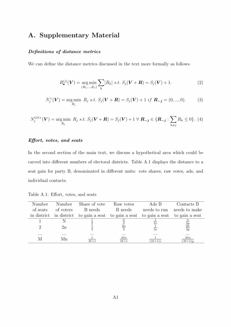
A. Supplementary Material

Definitions of distance metrics

We can define the distance metrics discussed in the text more formally as follows.

R(j)• (V ) = arg min

(R1,...,RJ )

∑h

|Rh| s.t. Sj(V + R) = Sj(V ) + 1. (2)

N+j (V ) = arg min

Rj

Rj s.t. Sj(V + R) = Sj(V ) + 1 if R−j = (0, ..., 0). (3)

NGS+j (V ) = arg min

Rj

Rj s.t. Sj(V +R) = Sj(V ) + 1 ∀ R−j ∈ {R−j :∑h6=j

Rh ≤ 0}. (4)

Effort, votes, and seats

In the second section of the main text, we discuss a hypothetical area which could be

carved into different numbers of electoral districts. Table A.1 displays the distance to a

seat gain for party B, denominated in different units: vote shares, raw votes, ads, and

individual contacts.

Table A.1: Effort, votes, and seats

Number Number Share of vote Raw votes Ads B Contacts Bof seats of voters B needs B needs needs to run needs to make

in district in district to gain a seat to gain a seat to gain a seat to gain a seat1 N 1

2n2

12z

n2y

2 2n 13

2n3

13z

2n3y

... ... ... ... ... ...M Mn 1

M+1MnM+1

1(M+1)z

Mn(M+1)y

A1

Vote shares, raw votes, or vote shares per seat?

The main text also discusses the units in which vote distances should be expressed—

vote shares, raw votes, or vote shares per seat—if they are to reflect cost distances. To

elaborate on that discussion, suppose that the technology of mobilization is scalable. In

this case, we can approximate Equation (1) as follows:

MBE =

(increment in vote share

ad

)(increment in seat share

increment in vote share

)Mb (5)

By assumption, the first term is z. Let n+j =

N+j

V•be the minimum vote share gain

that j needs to win another seat.21 Then the second term can be approximated as (1/M)

n+j

,

since the party gains a seat share of 1/M when it gains a vote share of n+j . Substituting

and simplifying, we find that MBE = zb/n+j . In other words, the MBE is proportional

to the reciprocal of the distance n+j , which is denominated in vote shares.

Now suppose that mobilization consists of contacting individual voters. In this case,

the first term in Equation (5) should be replaced by(increment in vote share

contact

).

By assumption, the increment in vote share per contact would be y votes out of V•,

or y/V•. Substituting and simplifying, we find that MBE = b/N+j . Thus, in this case,

the MBE is proportional to the reciprocal of the distance N+j , which is denominated in

raw votes.

21One could alternatively use R(j)• or NGS+

j , rather than N+j , in these calculations.

A2

B. Supplementary Analyses

0.0

5.1

.15

.2Vi

sit b

y ca

mpa

ign

wor

ker

4 6 8 10 12 14M

Norway

0.0

5.1

.15

.2C

onve

rsat

ion

with

can

dida

te

1 5 10 15 20 25 30 35M

Switzerland

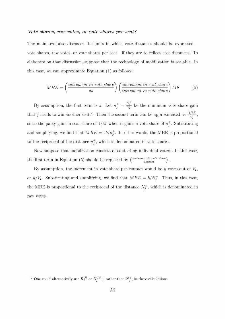
Figure B.1: Direct contact and district magnitude: survey evidence of the use ofnon-scalable mobilization technologyNote: The figure shows the relationship between a non-scalable mobilization technology—direct contact by campaign

workers and candidates—and district magnitude, with a non-linear model fitted to the data. This figure complements the

linear fit model presented in the main text as Figure 2. The left-hand panel uses data from the 1965-1969 Norwegian

Election Studies surveys (N=3,099) made available by Norwegian Center for Research Data (NSD). Respondents were

asked whether any party’s campaign worker visited them during the campaign. The right-hand panel uses data from the

1987-1991 Swiss National Election Studies surveys (N=1,895) made available by the Swiss Centre of Expertise in the Social

Sciences (FORS). Respondents were asked if they made use of conversations with candidates as information regarding the

election campaign. In each panel, we show binned scatterplots residualized by year fixed effects and survey respondent

background characteristics (age, gender, education level, and marital status).

B1

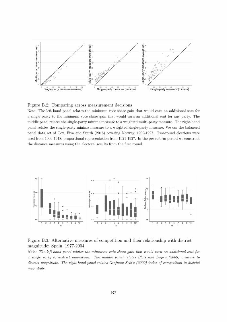
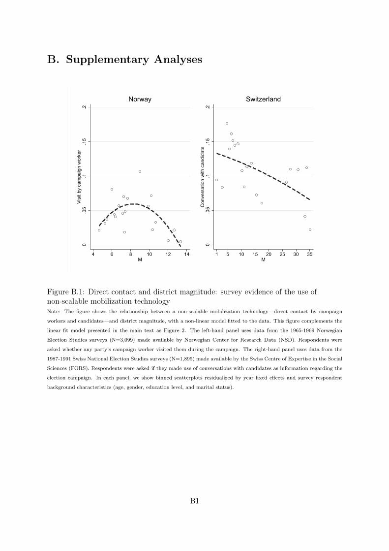
0.0

2.0

4.0

6.0

8.1

.12

.14

Mul

ti-pa

rty m

easu

re (m

inim

a)

0 .02 .04 .06 .08 .1 .12 .14

Single-party measure (minima)0

.02

.04

.06

.08

.1.1

2.1

4M

ulti-

party

mea

sure

(wei

ghte

d)0 .02 .04 .06 .08 .1 .12 .14

Single-party measure (minima)

0.0

2.0

4.0

6.0

8.1

.12

.14

Sing

le-p

arty

mea

sure

(wei

ghte

d)

0 .02 .04 .06 .08 .1 .12 .14

Single-party measure (minima)

Figure B.2: Comparing across measurement decisionsNote: The left-hand panel relates the minimum vote share gain that would earn an additional seat for

a single party to the minimum vote share gain that would earn an additional seat for any party. The

middle panel relates the single-party minima measure to a weighted multi-party measure. The right-hand

panel relates the single-party minima measure to a weighted single-party measure. We use the balanced

panel data set of Cox, Fiva and Smith (2016) covering Norway, 1909-1927. Two-round elections were

used from 1909-1918, proportional representation from 1921-1927. In the pre-reform period we construct

the distance measures using the electoral results from the first round.

0.1

.2.3

Trad

ition

al m

easu

re

1 2 3 4 5 6 7 8 9 10+M

0.2

.4.6

Blai

s-La

go m

easu

re

1 2 3 4 5 6 7 8 9 10+M

.2.4

.6.8

1G

rofm

an-S

elb

mea

sure

1 2 3 4 5 6 7 8 9 10+M

Figure B.3: Alternative measures of competition and their relationship with districtmagnitude: Spain, 1977-2004Note: The left-hand panel relates the minimum vote share gain that would earn an additional seat for

a single party to district magnitude. The middle panel relates Blais and Lago’s (2009) measure to

district magnitude. The right-hand panel relates Grofman-Selb’s (2009) index of competition to district

magnitude.

B2

.2.4

.6.8

1Tu

rnou

t


SMDs

.2.4

.6.8

1Tu

rnou

t


SMDs

.2.4

.6.8

1Tu

rnou

t


SMDs

.2.4

.6.8

1Tu

rnou

t


MMDs

.2.4

.6.8

1Tu

rnou

t


MMDs

.2.4

.6.8

1Tu

rnou

t


MMDs

Figure B.4: Alternative measures of competition and their relationship with voterturnout in SMDs and MMDs: Spain, 1977-2004Note: The figure relates voter turnout to three alternative measures of competition. In the top panel the

x-axes display the minimum vote share gain that would earn an additional seat for a single party. In the

middle panel the x-axes display Blais and Lago’s (2009) measure. In the bottom panel the x-axes display

Grofman-Selb’s (2009) index of competition.

B3

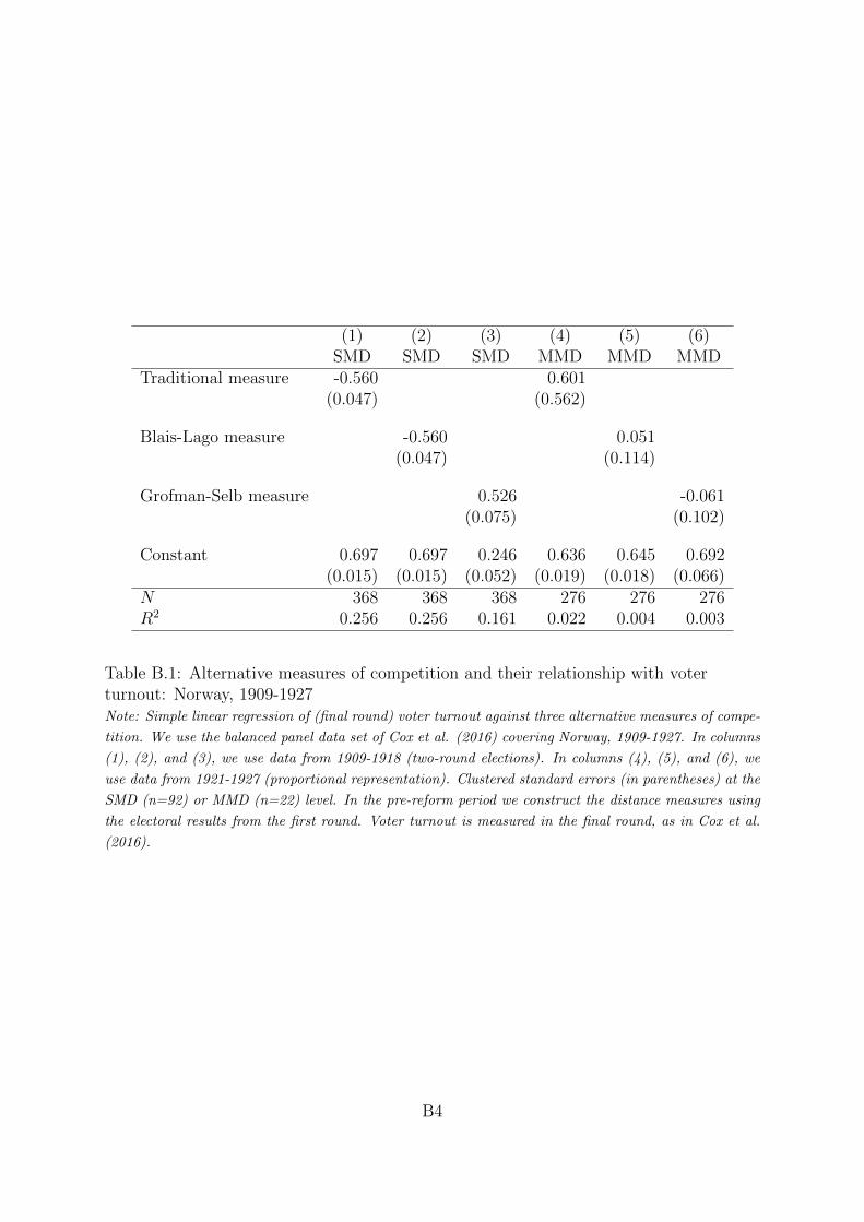
(1) (2) (3) (4) (5) (6)SMD SMD SMD MMD MMD MMD

Traditional measure -0.560 0.601(0.047) (0.562)

Blais-Lago measure -0.560 0.051(0.047) (0.114)

Grofman-Selb measure 0.526 -0.061(0.075) (0.102)

Constant 0.697 0.697 0.246 0.636 0.645 0.692(0.015) (0.015) (0.052) (0.019) (0.018) (0.066)

N 368 368 368 276 276 276R2 0.256 0.256 0.161 0.022 0.004 0.003

Table B.1: Alternative measures of competition and their relationship with voterturnout: Norway, 1909-1927Note: Simple linear regression of (final round) voter turnout against three alternative measures of compe-

tition. We use the balanced panel data set of Cox et al. (2016) covering Norway, 1909-1927. In columns

(1), (2), and (3), we use data from 1909-1918 (two-round elections). In columns (4), (5), and (6), we

use data from 1921-1927 (proportional representation). Clustered standard errors (in parentheses) at the

SMD (n=92) or MMD (n=22) level. In the pre-reform period we construct the distance measures using

the electoral results from the first round. Voter turnout is measured in the final round, as in Cox et al.

(2016).

B4

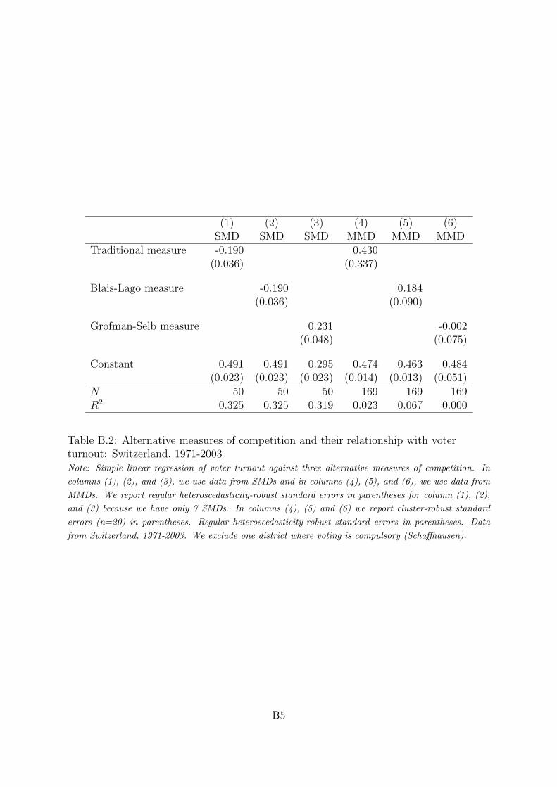
(1) (2) (3) (4) (5) (6)SMD SMD SMD MMD MMD MMD

Traditional measure -0.190 0.430(0.036) (0.337)

Blais-Lago measure -0.190 0.184(0.036) (0.090)

Grofman-Selb measure 0.231 -0.002(0.048) (0.075)

Constant 0.491 0.491 0.295 0.474 0.463 0.484(0.023) (0.023) (0.023) (0.014) (0.013) (0.051)

N 50 50 50 169 169 169R2 0.325 0.325 0.319 0.023 0.067 0.000

Table B.2: Alternative measures of competition and their relationship with voterturnout: Switzerland, 1971-2003Note: Simple linear regression of voter turnout against three alternative measures of competition. In

columns (1), (2), and (3), we use data from SMDs and in columns (4), (5), and (6), we use data from

MMDs. We report regular heteroscedasticity-robust standard errors in parentheses for column (1), (2),

and (3) because we have only 7 SMDs. In columns (4), (5) and (6) we report cluster-robust standard

errors (n=20) in parentheses. Regular heteroscedasticity-robust standard errors in parentheses. Data

from Switzerland, 1971-2003. We exclude one district where voting is compulsory (Schaffhausen).

B5