Embed Size (px)
Citation preview
The Computational Modeling of Baffle Configuration in the Primary Sedimentation Tanks
Mahdi Shahrokhi School of Civil Engineering Universiti Sains Malaysia Pulau Penang, Malaysia
Fatemeh Rostami School of Civil Engineering Universiti Sains Malaysia Pulau Penang, Malaysia [email protected]
Md Azlin Md Said School of Civil Engineering Universiti Sains Malaysia Pulau Penang, Malaysia
Syafalni School of Civil Engineering Universiti Sains Malaysia Pulau Penang, Malaysia [email protected]
Abstract— It is essential to have a uniform flow field for a settling tank with high performance. In general, however, the recirculation zones always appear in the sedimentation tanks. The non-uniformity of the velocity field, the short-circuiting at the surface and the motion of the jet at the bed of the tank that occurs because of the recirculation in the sedimentation layer, are affected by the geometry of the tank. One way to decrease the size of dead zone is using a suitable baffle configuration. In the first part of this study, the proper place of a single baffle in the tank was investigated numerically and in the next step the effect of existence of second baffle in the tank was tested. The results indicate that, the best position of the baffle is obtained when the volume of the recirculation region is minimized or is divided to smaller part and the flow field trend to be uniform in the settling zone to dissipate the kinetic energy in the tank.
Keywords- Sedimentation Tanks, Baffle Configuration, Computational Modeling.
I. INTRODUCTION The removal of suspended and colloidal materials from
water and wastewater by gravity separation (sedimentation) is one of the most widely used unit operations in water and wastewater treatment. The two main types of sedimentation tanks are primary and secondary settling tanks. A primary settling tank has low influent concentration. Its flow field is minimally influenced by the concentration field, and its buoyancy effects can be negligible. Secondary settling tanks, however, have higher influent concentration [1].
The recirculation (or dead) zones always appear in the sedimentation tanks. The presence of these regions may have various effects. There are some ways to decrease the size of the dead zones, which would increase the performance. Using a transverse baffle can reduce the effects of these factors, and enhance sedimentation performance [2].
Crosby [3] observed that a mid-radius baffle extending from the floor up to mid-depth decreased the effluent SS concentration of the clarifier by 37.5%. Zhou et al. [4] applied numerical modeling in studying the performance of circular secondary clarifiers with reaction baffles under
varying solid and hydraulic loadings. The importance of a baffle in dissipating the kinetic energy of incoming flow and reducing short circuiting indicates that the location of the baffle has a pronounced effect on the nature of the flow.
Huggins et al. [5] tested a number of potential raceway design modifications, noticed that by adding a baffle, the overall percentage of solid removal efficiency increased from 81.8% to 91.1%. Fan et al. [6] observed that the solid concentration profile in the flow region near the baffle is similar to that obtained without a baffle. By contrast, solid concentration increases sharply in the outer region of the baffle, which suggests that the solid phase congregates rapidly at the end of the baffle. Tamayol et al. [7] found that the best position for the baffle is somewhere in the circulation zone to spoil this circulation region.
Goula et al. [8] used numerical modeling to study particle settling in a sedimentation tank equipped with a vertical baffle installed at the inlet zone. The authors showed that the baffle increased particle settling efficiency from 90.4% for a standard tank without a baffle to 98.6% for a tank with an installed baffle. Installing baffles improves the performance of a tank in terms of settling. The baffles act as barriers, effectively suppressing the horizontal velocities of the flow and forcing the particles to the bottom of the basin [9].
The main objective of this study is to determine the favorable position of one and two baffles in a rectangular primary sedimentation tank. The investigations of the baffles position effect on the settling efficiency are performed via simulation using Flow-3D. Because comprehensive standards are not available for the design of baffle positions, the best baffle location is determined through numerical methods. The numerical experiments are performed for installation distances from the inlet of the tank. The results of the numerical modeling show that primary sedimentation tank performance can be improved by altering the geometry of the tank and the effects of baffle on the efficiency of the primary sedimentation tank are investigated via assessment of the circulation zone volume variations and the magnitude of the kinetic energy in the flow field.
V2-392
2011 2nd International Conference on Environmental Science and Technology IPCBEE vol.6 (2011) © (2011) IACSIT Press, Singapore
II. COMPUATIONAL MODEL
A. Mathematical model Steady state incompressible flow conditions with viscous
effect are generally considered in hydraulic numerical modeling, and the Navier–Stokes equation has been well-verified as an effective solution to the governing equation. The Navier–Stokes equation is an incompressible form of the conservation of mass and momentum equations, and is comprised of non-linear advection, rate of change, diffusion, and source term in the partial differential equation. The mass and momentum equations joined by velocity can be used to obtain an equation for the pressure term. When the flow field is turbulent, computation becomes more complex. Because of this, the Reynolds-Averaged Navier–Stokes (RANS) equation is prevalently used. It is a modified form of the Navier–Stokes equation and includes the Reynolds stress term, which approximates the random turbulent fluctuations by statistics.
The governing equations are general mass continuity and momentum. The turbulence model is also solved with these equations to calculate the Reynolds stresses. The governing equation in two-dimensional flow in the x and z directions is presented here. The general mass continuity equation is [10, 11]:
( ) ( ) 0f x zV uA wAt x z
ρρ ρ
∂ ∂ ∂+ + =
∂ ∂ ∂ (1)
where fV is the fractional volume of flow in the calculation cell; ρ is the fluid density; and (u,w) are the velocity components in the length and height (x,z). The momentum equation for the fluid velocity components in the two directions are the Navier–Stokes equations, expressed as follows:
{ }1 1 x z x x
f
u u u PuA wA G f
t V x z xρ∂ ∂ ∂ ∂
+ + = − + +∂ ∂ ∂ ∂
(2)
{ }1 1x z z z
f
w w w PuA wA G f
t V x z zρ∂ ∂ ∂ ∂
+ + = − + +∂ ∂ ∂ ∂
(3)
where Gx,Gz are body accelerations, and fx,fz are viscous accelerations. Variable dynamic viscosity µ are as follows:
( ) ( ){ }f x x xx z xzV f wsx A Ax z
ρ τ τ∂ ∂
= − +∂ ∂
(4)
( ) ( ){ }f z x xz z zzV f wsz A Ax z
ρ τ τ∂ ∂
= − +∂ ∂
(5)
where,
{ }2 , 2 ,x xzzx z
u w u w
x z z xτ μ τ μ τ μ
∂ ∂ ∂ ∂= − = − = − +
∂ ∂ ∂ ∂
In the above expressions, the terms wsx and wsz are wall shear stresses. If these terms are omitted, there is no wall shear stress because the remaining terms contain the fractional flow areas (Ax, Az) which vanish at walls. The wall stresses are modeled by assuming a zero tangential velocity on the portion of any area closed to flow. Mesh boundaries are an exception because they can be assigned non-zero tangential velocities. For turbulent flows, a law-of-the-wall velocity profile is assumed near the wall, which modifies the wall shear stress magnitude [12].
Fluid surface shape is illustrated by volume-of-fluid (VOF) function F(x, z, t). With the VOF method, grid cells are classified as empty, full, or partially filled with fluid. Cells are allocated in the fluid fraction varying from zero to one, depending on fluid quantity. Thus, in F=1, fluid exists, whereas F=0 corresponds to a void region. This function displays the VOF per unit volume and satisfies the equation [10].
( ) ( ){ }10x z
F
FFA u FA w
t V x z
∂ ∂ ∂+ + =
∂ ∂ ∂ (6)
F in one phase problem depicts the volume fraction filled by the fluid. Voids are regions without fluid mass that have a uniform pressure appointed to them. Physically, they represent regions filled with vapor or gas, whose density is insignificant in relation to fluid density.
B. Numerical solver In this paper, a numerical flow solver (Flow-3D, version
9.4.1), which utilizes a finite volume scheme for structured meshes, is used to simulate the free surface flow in these tanks. The flow field is separated into fixed rectangular cells. The local average values of all dependent variables for each cell are computed. Pressures and velocities are associated implicitly by using time-advanced pressures in momentum equations and time-advanced velocities in the mass (continuity) equation. These semi-implicit formulations of the finite-difference equations enable the efficient resolution of low speed and incompressible flow problems. The semi-implicit formulation, however, results in coupled sets of equations that must be solved by an iterative technique [12].
Flow-3D solves the RANS equations by the finite volume formulation gained from a rectangular finite difference grid. For each cell, mean values of the flow parameters, such as pressure and velocity, are calculated at discrete times. The new velocity in each cell is computed from the coupled momentum and continuity equation using previous time step values in each of the centers of the cell faces. The pressure term is obtained and adjusted using the estimated velocity to satisfy the continuity equation. With the computed velocity and pressure for a later period, the remaining variables are estimated involving turbulent
V2-393
transport, density advection and diffusion, and wall function evaluation [12].
In the utilized software, the Fractional Area/Volume Obstacle Representation (FAVOR) method can be used to inspect the geometry in the finite volume mesh [11]. FAVOR appoints the obstacles in a calculation cell with a factional value between zero to one as obstacle fills in the cell. The geometry of the obstacle is placed in the mesh by setting the area fractions on the cell faces along with the volume fraction open to flow [13]. This approach creates an independent geometry structure on the grid, and then the complex obstacle can be produced.
III. VERIFICATION TEST In order to verify the results of computational model, an
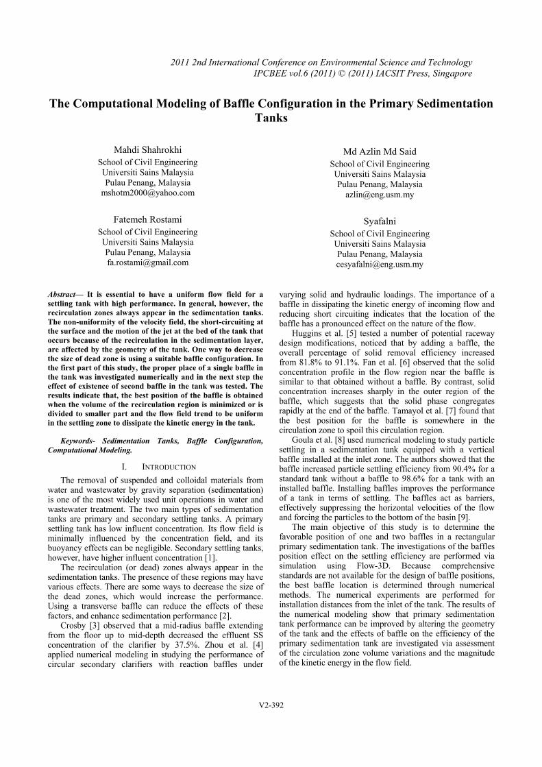
experiment was carried out in a settling tank with length of 200 cm, depth of 30 cm, wide of 50cm, an opening inlet of 10 cm, and a flow rate of 2 lit/s. The velocity field in the settling tank was measured by means of Acoustic Doppler Velocimeter (ADV).
A 10 MHz Nortek ADV is used for measuring instantaneous velocities of the liquid flow at different points in the tank. The ADV uses the Doppler effects to measure current velocity by transmitting short pairs of sound pulses, listening to their echoes and, ultimately, measuring the change in pitch or frequency of the returned sound. Sound does not reflect from the water itself, but rather from particles suspended in the water. The ADV uses four receivers, all focused on the same volume, to obtain the three velocity components from that very volume. The accuracy of the measured data is no greater than ±0.5% of measured value ± 1 mm/s [14].
Flow field in sedimentation tanks is three-dimensional. The degree of importance of the three-dimensional effects is related to the place of the baffles, inlet and outlet of a basin and their widths. The baffles, inlet and outlet are assumed to uniformly extend the width of the basins, making the three-dimensional effects unimportant. For simplicity, two-dimensional models were used for the simulations.
In this study, the rectangular mesh with 288×69 grids was applied for the computation. Thus, the mesh with approximately 19872 cells was used. To calculate turbulence effects on the flow field, the k-ε turbulence model was selected. In this study, the flow is clear and has no particles. Fig. 1 shows a comparison between the results of the numerical models and experiments data. From Fig. 1, the numerical model predicts accurate data in comparison with experiments.
IV. COMPUTATIONAL INVESTIGATIONS The boundary condition for the inflow (influent) is
constant velocity, and outflow condition was selected for the outlet (effluent). No slip conditions were applied at the rigid walls, and these were treated as non-penetrative boundaries. A law-of-the-wall velocity profile was assumed near the wall, which modifies the wall shear stress magnitude. Free surface boundary was calculated by the VOF method.
ο Experimental data, ― Numerical data
Figure 1. Comparison of velocity profiles of numerical and experimental study for a tank without baffle.
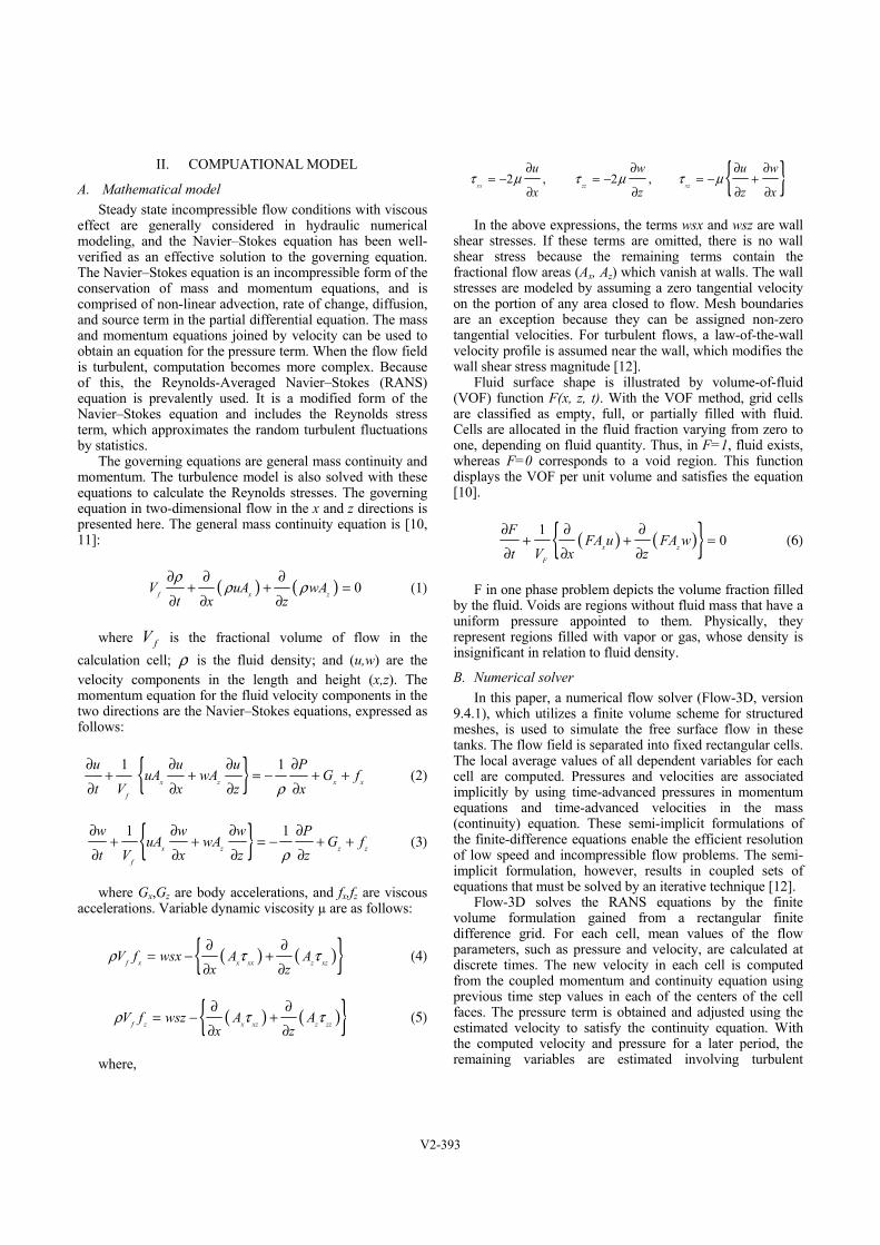
A. Proper position of one baffle The geometry of the longitudinal sedimentation tank with
a baffle is illustrated in Fig. 2(a). The same basin in section III was applied. A weir is located at the end of the basin to regulate the flow height of H=30 cm. Baffle height a=5.5 cm. The inlet flow goes through a sluice gate with an opening of hin=10 cm. The numerical experiments were conducted for eight positions of baffle for the same flow rate (equal to Q=2 lit/s). Case 1 is for no baffle (same as section III) and in cases 2 to 9, a baffle is located in various distances from the inlet to tank length ratio, d/L=0.10, 0.125, 0.135, 0.150, 0.20, 0.250, 0.30 and 0.40.
Figure 2. Schematic diagram of the tank for (a) one baffle and (b) two
baffles in the tank.
The best location for the baffle is obtained when the volume of the circulation zone is minimized or the recirculation region forms a small portion of the flow field. Therefore, the best position for the baffle may lead to a more uniform distribution of velocity in the tank and minimize dead zones.
Different baffle positions were modelled in this study. Circulation volume, which is normalized by the total water volume in the tank and calculated by the numerical method, is shown in Table I. The table indicates the absolute predictability of some cases to exhibit weak performance because of the size of the dead zone. Table I shows that the baffle position at d/L=0.125 has minimum magnitude of circulation volume and consequently exhibits the best performance. In addition, this table indicate that if baffle is
(a)
(b)
u /U in-1 0 1 2
x = 4 6 c m
u /U in-1 0 1 2
x = 1 4 9 c m
u /U in
z/H
in
-1 0 1 20
0 .5
1
1 .5
2
2 .5
3
3 .5
x = 1 0 c m
u /U in-1 0 1 2
x = 8 2 c m
u /U in- 1 0 1 2
x = 1 1 8 c m
u /U in-1 0 1 2
x = 1 9 0 c m
H=30 cm
L=200 cm
hin=10 cm
d
H=30 cm
L=200 cm
hin=10 cm
25 cmd
V2-394
B
located in woless than a tnecessary toconfiguration
Furthermbaffle distanczone graduaefficiency of t
TABLE I.
d/L 0.10
C.V. % 33.9
B. Proper poThe suitab
tank is studid/L=0.125 anto find the be2(b). Circulatwater volumemethod is shobaffle in settzone clearly. From this tabS/L = 0.125, 0the second bacan effect on tank and creadeposition of
TABLE II.
d/L
C.V. %
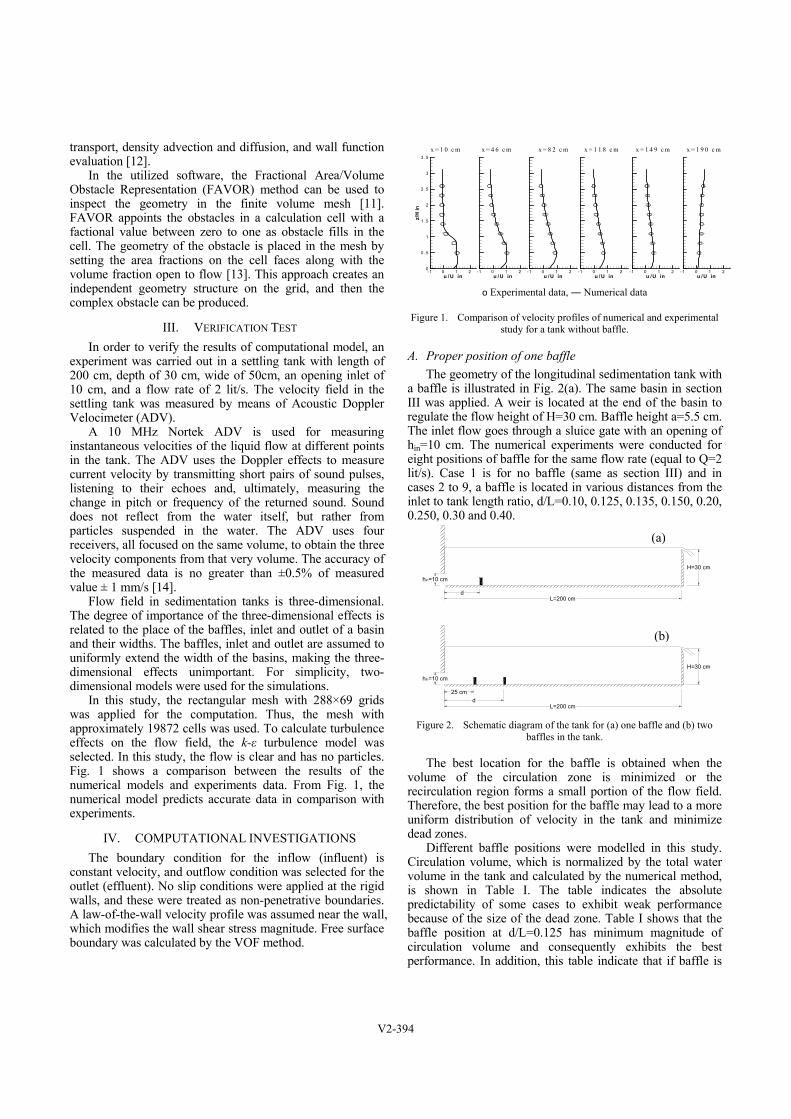
C. Flow patteComputed
baffles at thecase no bafflethe settling tavolume of thewith one and remains minimdead zone intcases one and30.0 percent othis means thsize of circusedimentationnumber leadsthe added baff
orse position, tank without
o investigate of the baffle i
more, Table I e from point d
ally increasethe tank also d
CIRCULATIONLOCATIO
0.125
0.135
32.3 34.1
osition of two bble place of sed in this sed different locest position otion volume we in the tank ows in Table ling tank canBut the positle it is absolut0.388 have theaffle spoils theincreasing theate calm flowthe suspended
CIRCULATIONLOCATION
0.256 0.300
30.9 30.6
ern in the sedd streamlines fe optimum poe a large circulank which oce tank. Two ctwo baffles. T
mized and theto two sectiond two baffles of the total vohat increasing ulation regionn process. In os to diminishinffle.
the efficiencyany baffle. about the
in settling tankillustrates th
d/L=0.125, thes. Consequedecreases.
N VOLUME PERCEON OF ONE BAFFLE
0.15
0.20
0.5
34.4 34.4 35
d : The baffle
L : The length of th
baffles econd baffle
ection. The fications of secoof second baffwhich is normand calculateII. This table
n decrease siztion of bafflestely predictabe best performe dead zone oe sedimentatio
w that reach tod solids.
N VOLUME PERCEOF SECOND BAFF
0.388 0.519
30.0 30.4
dimentation tanfor case of no
osition are sholation zone exccupies 37.1 circulation zonThe circulatioe baffle presu
ns. Two vortic in Fig. 3 wh
olume of the tathe number
n and conseqother words adng the height
y of this tank Consequentlybest positio
k. hat with incre volume of thently, the re
ENTAGE IN DIFFERE
.25
0.30
0.40
5.1 35.5 37.8
distance from the inlet
he tank, C.V. : Circulati
in the sedimeirst baffle plaond baffle wasfle as shown malized by thed by the nume illustrate thaze of the circs is more imple that two ba
mance. In otherof the first bafon area in the so better locat
ENTAGE IN DIFFERFLE
One Baffle
No-Baffl
32.3 37.1
nks o baffle, one aown in Fig.3. xists in the surpercent of thnes exist in thon volume, houmably separaes are shown hich spoils 32ank, respectivof baffle redu
quently improddition of the b
of the vortice
maybe y, it is on and
reasing he dead emoval
RENT
No- Baffl
e
37.1
t of the tank
ion Volume
entation aces at s tested in Fig.
he total merical
at using culation portant. affles at r words, ffle and settling ion for
RENT
le
and two In the
rface of he total he tank owever, ates the for the
2.3 and vely. So uce the ove the baffle’s es after
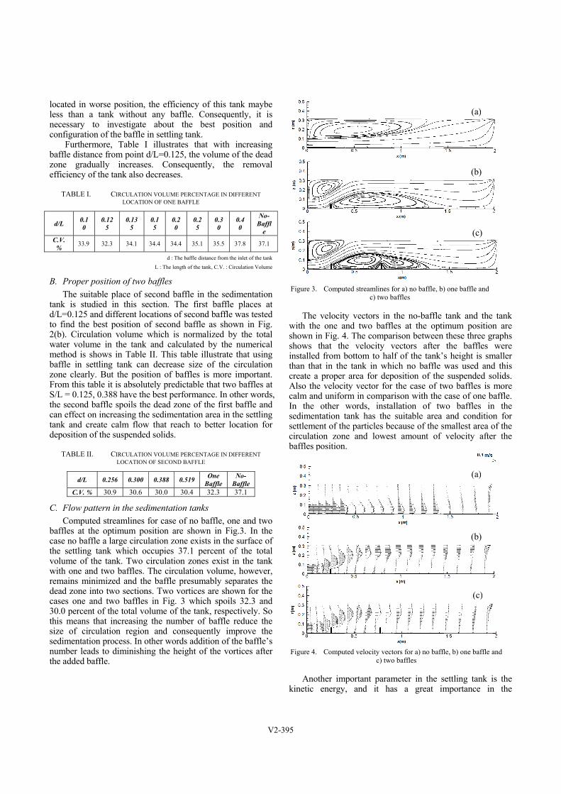
Fi
wishshinthcrAlcaInsesecirba
Fi
ki
igure 3. Compu
The velocityith the one a
hown in Fig. 4hows that thnstalled from bhan that in thereate a proper lso the veloci
alm and uniforn the other edimentation tettlement of thrculation zonaffles position
igure 4. Comput
Another imnetic energy
ted streamlines foc) two ba
y vectors in tand two baffle4. The compare velocity vbottom to halfe tank in whi
area for depoity vector for rm in compariwords, instaltank has the
he particles bene and lowest.
ted velocity vectoc) two
mportant param, and it has
or a) no baffle, b)affles
the no-baffle es at the optirison between vectors after f of the tank’ch no baffle osition of thethe case of twison with the llation of twsuitable area cause of the st amount of
ors for a) no baffl baffles
meter in the ss a great im
) one baffle and
tank and the imum positionthese three grthe baffles
s height is smwas used and suspended sowo baffles is case of one b
wo baffles inand condition
smallest area ovelocity after
fle, b) one baffle a
settling tank importance in
(a)
(b)
(c)
(a)
(b)
(c)
tank n are raphs were
maller d this olids. more affle.
n the n for of the r the
and
is the n the
V2-395
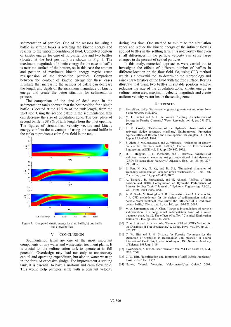
sedimentation of particles. One of the reasons for using a baffle in settling tanks is reducing the kinetic energy and reaches to the uniform condition of fluid. Computed contour of kinetic energy for case of no baffle, one and two baffles (located at the best position) are shown in Fig. 5. The maximum magnitude of kinetic energy for the case no baffle is near the surface of the bottom, so in this case the amount and position of maximum kinetic energy maybe cause resuspension of the deposition particles. Comparison between the contour of kinetic energy for these cases illustrate that increasing the number of baffle can decrease the length and depth of the maximum magnitude of kinetic energy and create the better situation for sedimentation process.
The comparison of the size of dead zone in the sedimentation tanks showed that the best position for a single baffle is located at the 12.5 % of the tank length, from the inlet slot. Using the second baffle in the sedimentation tank can decrease the size of circulation zone. The best place of second baffle is 38.8% of tank length from the inlet opening. The figures of streamlines, velocity vectors and kinetic energy confirm the advantage of using the second baffle in the tanks to produce a calm flow field in the tank.
Figure 5. Computed kinetic energy for a) no baffle, b) one baffle
and c) two baffles
V. CONCLUSION Sedimentation tanks are one of the most important
components of any water and wastewater treatment plants. It is crucial for the sedimentation tank to operate at its full potential. Overdesign may lead not only to unnecessary capital and operating expenditure, but also to water wastage in the form of excessive sludge. For improvement a settling tank, it is essential to have a uniform and calm flow field. This would help particles settle with a constant velocity
during less time. One method to minimize the circulation zones and reduce the kinetic energy of the influent flow is applied baffles in the settling tank. It is noteworthy that even small differences in the particle velocity can cause large changes in the percent of settled particles.
In this study, numerical approaches were carried out to investigate the effects of different number of baffles in different location on the flow field. So, using CFD method which is a powerful tool to determine the morphology and raise characteristics of the fluid with the free surface. Results illustrate that using two baffles in suitable position achieve reducing the size of the circulation zone, kinetic energy in sedimentation area, maximum velocity magnitude and create uniform velocity vector inside the settling zone.
REFERENCES [1] Metcalf and Eddy, Wastewater engineering treatment and reuse. New
York: McGraw-Hill, 2003. [2] M. J. Hamlan and A. H. A. Wahab, "Settling Characteristics of
Sewage in Density Currents," Water Research, vol. 4, pp. 251-271, 1970.
[3] R. M. Crosby, "Evaluation of the Hydraulic characteristics of activated sludge secondary clarifiers," Environmental Protection Agency,Office of Research and Development, Washington, D.C. U.S Report EPA-600/2, 1984.
[4] S. Zhou, J. McCorquodale, and Z. Vitasovic, "Influences of density on circular clarifiers with baffles," Journal of Environmental Engineering, ASCE, vol. 118, pp. 829-847, 1992.
[5] D. L. Huggins, R. H. Piedrahita, and T. Rumsey, "Analysis of sediment transport modeling using computational fluid dynamics (CFD) for aquaculture raceways," Aquacult. Eng., vol. 31, pp. 277-293, 2005.
[6] L. Fan, N. Xu, N. Ke, and H. Shi, "Numerical simulation of secondary sedimentation tank for urban wastewater," J. Chin. Inst. Chem. Eng., vol. 38, pp. 425-433, 2007.
[7] A. Tamayol, B. Firoozabadi, and G. Ahmadi, "Effects of Inlet Position and Baffle Configuration on Hydraulic Performance of Primary Settling Tanks," Journal of Hydraulic Engineering, ASCE., vol. 134 pp. 1004-1009, 2008.
[8] A. M. Goula, M. Kostoglou, T. D. Karapantsios, and A. I. Zouboulis, " A CFD methodology for the design of sedimentation tanks in potable water treatment case study: the influence of a feed flow control baffle," Chem. Eng. J., vol. 140, pp. 110-121, 2007.
[9] M. A. Sammarraee and A. Chan, "Large-eddy simulations of particle sedimentation in a longitudinal sedimentation basin of a water treatment plant. Part 2: The effects of baffles," Chemical Engineering Journal vol. 152, pp. 315-321, 2009.
[10] C. W. Hirt and B. D. Nichols, "Volume of Fluid (VOF) Method for the Dynamics of Free Boundaries," J. Comp. Phys., vol. 39, pp. 201-225, 1981.
[11] C. W. Hirt and J. M. Sicilian, "A Porosity Technique for the Definition of Obstacles in Rectangular Cell Meshes," in Fourth International Conf. Ship Hydro. Washington, DC: National Academy of Science, 1985, pp. 1-19.
[12] FlowScience, "Flow-3D user manual," Ver. 9.4.1 ed Santa Fe, NM, USA, 2009.
[13] C. W. Hirt, "Identification and Treatment of Stiff Bubble Problems," Flow Science Inc., 1992.
[14] Nortek, "Nortek Vectorino Velocimeter-User Guide," 2004.
(a)
(b)
(c)
V2-396