The computation of deformations

The computation of deformations

Derek Flinn

The mathematics of irrotational deformation are simplified by presentation in matrix form. Matrix equations are easily programmed and are easily interpreted in geometrical terms. Graphical operations commonly carried out on orientation nets such as rotation of data can be translated into simple matrix equations for use with a computer. If the shape and orientation of the deformation ellipsoid for a pure shear are known, a matrix can be constructed for use as a deformation matrix. This can be used TO deform other deformation ellipsoids to obtain a resultant ellipsoid. It can also be used to deform geological structures such as lineations and planes. The matrix equations for these operations are very simple, but their numerical solution often requires a computer.

1. Introduction

Equations for the computation of deformations should be in a form which is suitable for programming and for numerical evaluation. It should also be easy to interpret them in geometrical terms in order for them to be of maximum use to structural geologists. A number of papers on the mathematics of deformation have been published in recent years. Most of those concerned with homogenous strain derive algebraic equations which do not take advantage of the methods developed by numerical analysis for avoiding the accumulation of rounding errors during numerical solution. The methods employed in obtaining these equations tend to be algebraic rather then geometric.

The importance to structural geology of a geometric approach is shown by a consideration of the history of the development of the subject. When Schmidt (1923) introduced the orientation net for the treatment of orientation data he began a revolution in structural geology. The orientation net can be used as an analogue computer to solve many problems in three-dimensional trigonometry. It is even more useful for the analysis of the distribution of orientation data and as an aid to three-dimensional thinking. It seems unlikely that a purely mathematical approach could have been as useful in structural geology.

Before the 1960’s deformation was rarely treated as three-dimensional. This must have been due less to ignorance of suitable algebraic methods than to the lack of a device such as the deformation plot which could be used, like the orientation net, as an aid to thinking in three-dimensional terms. The concept of the deformation ellipsoid had been familiar to geologists for a long time. However, relatively little use was made of it, despite the availability of mathematical and even graphical methods (Mohr’s representation) for operating with the ellipsoid. The deformation plot orders the infinite range of ellipsoids Geol. J. Vol. 14. Pt 1, 1979 87

a8 D. FLINN

into pattern which can be easily visualized. This simplifies the task of thinking about deformation in much the same way that the orientation net simplifies thinking about orientation in threedimensions.

Until now mathematical solutions to structural problems have been found after the solutions have been obtained intuitively by three-dimensional thinking aided by simple graphical devices. We now have to consider the problem of superposed deformations and from the complexity of the problem it seems possible that no simple graphical solution will be found. It is possible to use the logarithmic deformation plot to construct graphically the deformation paths of coaxial deformations, however complex, and even to visualise that construction; but for non-coaxial deformations the problem is much more difficult (Flinn 1978). It is the purpose of this paper to show that matrix algebra may be used to construct a set of very simple equations for computing irrotational homogeneous strain. They are not only eminently suitable for programming and for solution by the methods of numerical analysis but can also be interpreted in geometric terms based directly on field data. It will be assumed in what follows that the reader is conversant with the elementary rules and operations of matrix algebra including matrix multiplication, transposition, inversion and the manipulation of matrix equations. All the matrix algebra used below will be found in any elementary text book on matrices (e.g. Thompson 1969).

2. Computations with orientation data

The operations with structural directions which are commonly carried out on orientation nets have to be translated into mathematical operations for incorporation into computer programs and for the production of more precise results than can be obtained by graphical methods. For this purpose three orthogonal, equally scaled reference directions are defined as follows: +Z pointing to the zenith, +N to the north (true) and +E to the east. On the equatorial orientation net + z plots in the centre, +N at the north pole and +E at the right hand end of the equator.

These reference axes form a left-handed co-ordinate system in conformity with normal geological practice, thus allowing compass bearings and dip readings to be used without modification.

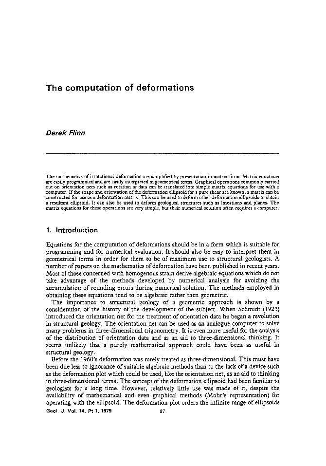
The orientation of structural directions such as axes, lineations and poles of planes are specified in terms of their projections on the three orthogonal axes in the order, 2, N, E with the reference axes intersecting in the direction concerned (Fig. 1). Such projections are called direction numbers. If they result from the projection of a unit length marked off from the intersection with the reference axes along the structural direction they are called direction cosines because they are numerically equal to the cosines of the angles between direction and the axes onto which it is projected.

For geological purposes the three direction cosines of a direction (I m njT=l are most conveniently obtained from

I=cos 8 m=sin 8 cos + n-sin 8 sin + (1)

where for poles of planes, 8 is the angle of dip of the plane and + is the azimuth of dip while for axes and lineations 8 is the dip and 8 is the azimuth of the axis or lineation. Here the dip of the axis or lineation is the angle from the zenith (90° +plunge) and is geometrically equivalent to the dip of a magnetic direction.

For direction cosines e.g. 1=(I m n ) T

Iz + m 2 + n 2 = 1

THE COMPUTATION OF DEFORMATIONS

I -:1 t

a

c

- L

b

N

Fig. 1. Reference axes (geological left-handed system) and direction cosines (a) perspective view of reference axes, 2, N, E and a vector of unit lengzh. y,, yI, y, direction an les of the unit vector. 8, $ dip and azimuth otthe unit vector. @) part of an equal-area net projection of (a).

but for direction numbers, e.g. I' =(I' m' n ' )T

1 ' 2 +m'2 +ntZ =j+l ( 3 ) During computation direction cosines are sometimes converted into direction numbers due to elongation, and then in order to be able to interpret them back into dips and azimuths it is necessary to normalise them into direction cosines as follows,

I = l ',f+ m = m'bi n = n ',$+ (4) where j is given by (3). Then they can be interpreted in angular form as follows,

0=arc cos 1 +=arctan (n/m)+90° (1-sign (m) ) (5) Operations commonly carried out on the orientation net can be computed as follows.

The angle, a, between any two directions specified in the form of direction cosines, 1 , = ( I , m, n , P , 1 , = v 2 m2 n2)P

is obtainedfrom c o s a = 1 , l 2 + m , m 2 + n , n 2 = 1 ~ l 2 (6) The direction cosines 1=(1 m n ) T of the direction which is normal to the two directions I , andl , are

I = m , n 2 - n l m 2 m=n,12 - l ,n , n=l,m, - 12m, (7)

90 D. FLINN

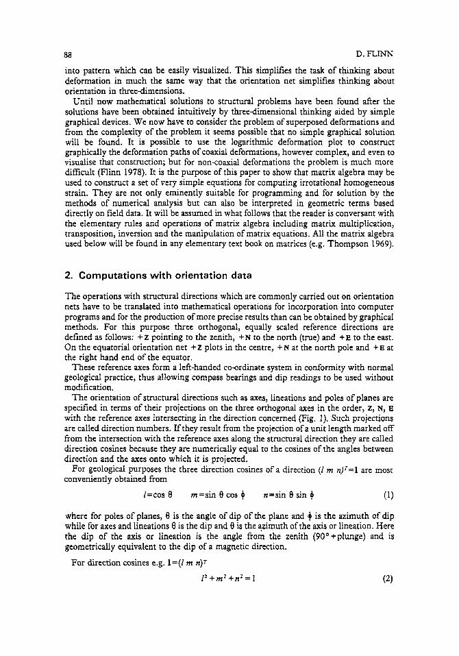
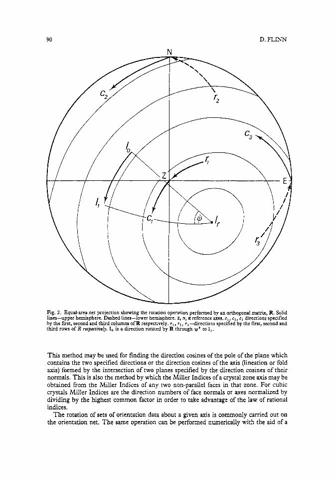
Fig. 2. Equal-area net projection showing the rotation operation performed by an onhogonal matrix, R. Solid lines-upper hemisphere. Dashed lines-lower hemisphere. z, H, E reference axes. c,, c2 , c, directions specified by the first, second and third columns of R respecrively. t,, t 2 , r, directions specified by the first, second and third rows of R respecriwdy. 1, is a direction rotated by R through y o to 1,.

This method may be used for finding the direction cosines of the pole of the plane which contains the two specified directions or the direction cosines of the axis (lineation or fold axis) formed by the intersection of two planes specified by the direction cosines of their normals. This is also the method by which the Miller Indices of a crystal zone axis may be obtained from the Miller Indices of any two non-parallel faces in that zone. For cubic crystals Miller Indices are the direction numbers of face normals or axes normalized by dividing by the highest common factor in order to take advantage of the law of rational indices.

The rotation of sets of orientation data about a given axis is commonly carried out on the orientation net. The same operation can be performed numerically with the aid of a

THE COMPUTATION OF DEFORMATIONS 91

3 x 3 orthogonal matrix, R. Orthogonal matrices have special properties. Each column and each row is a set of direction cosines and therefore obeys equation (2). Each pair of columns is related to the third column by equation (7), because the three directions represented by the columns are normal to each other. Therefore each pair of columns substituted into equation (6) gives a result of cos a = 0, Q = 90". The three rows are also three sets of orthogonal direction cosines which therefore behave in the same way.

The operation performed by an orthogonal matrix is pure rotation. A direction lo is rotated without change of length to a new orientation specified by the direction cosines 1 , as follows

11 =R1, (8)

The rotation matrix, R, can be interpreted as follows (Fig. 2). The columns of R are the direction cosines after the rotation of those directions which before the rotation were parallel to the reference axes. The rows of R are the direction cosines before the rotation of those directions which are parallel to the reference axes after the rotation.

The same matrix can produce the same rotation but in the opposite sense as follows

lT=l:R (84

when the rows of R give the destination of the reference axis directions after rotation and the columns give the origin of the reference axis directions before the rotation; the reverse of their roles in the previous operation, equation 8. The same rotation as given by equation 8a can be produced alternatively by

1 , =Rr l , (8b)

because the rows and columns of R have been interchanged relatively to equation 8. The rotation produced in equation 8 can be reversed after it has taken place by

1, =Rr 1, (84

because for orthogonal matrices Rr=R-' It should be noted that in equations 8, 8a, 8b and 8c, 1, represents a direction. If a plane

represented by the direction cosines of its normal (equation 1) is to be rotated then in equations 8 and 8a, R must be replaced by Rr and in equations 8b and 8c, Rr must be replaced by R.

The matrix R can be further interpreted in terms of the orientation of the axis about which rotation takes place and the angular amount of that rotation as follows (Fig. 2). The angle of rotation q~ is given by

cos yr=O.5 (tr (R) -1) (9)

where tr(R) is the sum of the elements in the leading diagonal of R, i.e. I , + m , + n 3 and the direction cosines of the axis of rotation are

if

92

N

D. FLINN

i n

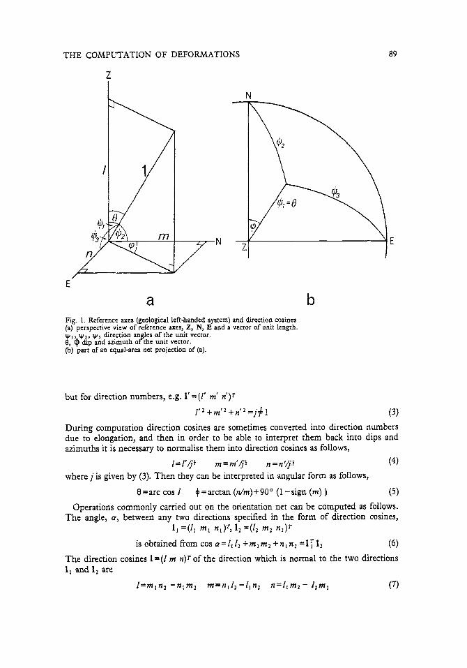
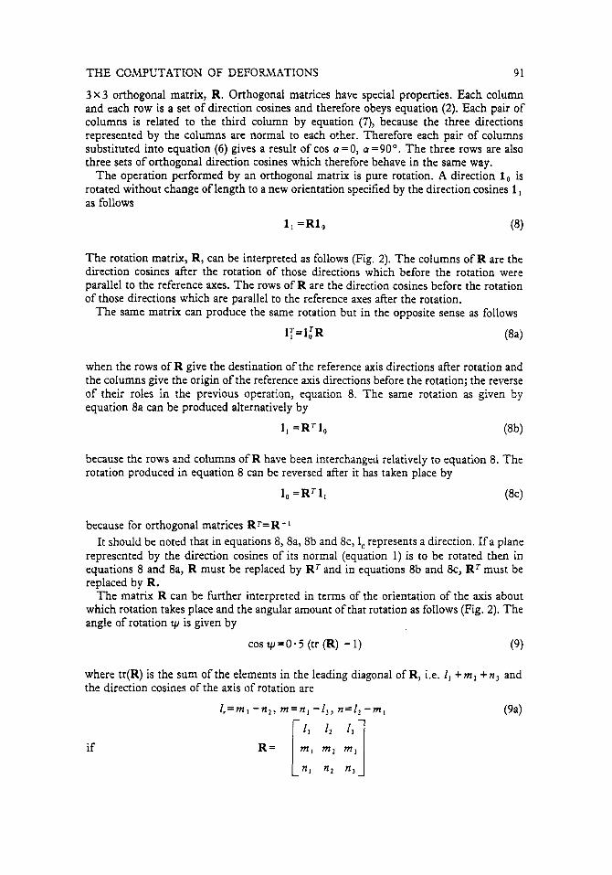
Fig. 3. Part ofan equal-area projection showing the rotations caused by the orthogonal matrices Rz, RN, RE (equations 10 in text). R,, R,, RE rotate the direction 1, to l,, l,, 1, respecrively.

If a rotation of v, clockwise towards the origin is to take place about z, N or E then the rotation matrix, R, simplifies to, respectively:

0

R,= [ i c o s y sinow ] R,= [ cO:w 8 1 -sin v, cos v, sin 4, cos v,

[ co;v, si;v, H 1; (10)

RB= -sin v, cos v,

The use of RZ in equation 8 is equivalent to rotation on the orientation net about its centre, which is most efficiently accomplished by moving the zero point on the tracing paper the appropriate number of degrees in the opposite direction to that in which the data is required to be moved. The use of R,is equivalent to moving the data points along lines of latitude on the net, and the use of Rgis equivalent to rotating the tracing paper 90°, moving the data points along the lines of latitude and then restoring the 90" rotation of the tracing paper (Fig. 3). It is clear that rotation about z is the most efficient graphical rotation.

If it is required to rotate a set of orientation data by a specified angle v, clockwise towards the origin about an axis, 1, inclined at 8" to z with an azimuth of 0 the operation can be done numerically in exactly the same way that it would be done on the orientation net.

The first step is to rotate the data about z so that 1, lies on the equator of the net. This requires the matrix, R, .


0 0 0 0

0 sin (0 - 90) cos (0 - 90) -cos + sin + The next step is to rotate the data about N until 1, is parallel to z using R,

cos 0 0 -sin 8

sin 0 0 cos 8 R , = [ 0 1

and then the data is rotated yo about z using R,

O 1

1 0 0 cos y sin y 0 -sin y cos y,

Finally the rotation due to R, is reversed followed by the reversal of the rotation due to R , . The total operation can be represented as follows:

1, =R:R:R, R2 R , I, =No (14) Thus the numerical rotation of data can be simplified by multiplying together the five rotation matrices to obtain a single rotation matrix. It should be noted that the sequence of operations employed above makes maximum use of the graphically simple rotation about z. This sequence differs from that recommended by Phillips (1960 p. 36) who employs the less efficient method of rotating 1, to the outside of the net in the third stage.

The columns and rows of R in equation 14 can be interpreted as direction cosines ofthe directions rotated to and from the reference axes as described above. Had either of these sets of directions been known in advance the matrix, R, could have been constructed directly.

It is essential for accurate numerical results that the matrix used for rotation be exactly orthonormal. Sets of “orthogonal” directions read off the orientation net, unless at least one direction is parallel to a reference axis, are never sufficiently orthogonal to provide truly orthogonal matrices. A procedure for the orthonormalisation of matrices can be obtained from part of the sequence of operations derived above for rotation about an oblique axis.

The columns of the matrix to be orthogonalized are rearranged so that the column whose direction is most reliably known becomes the first column and the second column becomes the second most reliable known direction giving the matrix M.

cos 0 I, M- [ sin e cos + ;: i3 ]

sin 8 sin + M is then rotated so that the direction represented by the first column lies paraIIel to 2, giving the matrix Mi . Numerically this requires the first two steps of the sequence given above, equations 11 and 12:

M,=R, R , M

94 D. FLINN

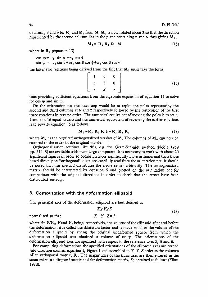
obtaining 0 and 4 for R2 and R, from M. M I is now rotated about zso that the direction represented by the second column lies in the plane containing z and N thus giving M, .

M,= R, R, R, M (15) where in R3 (equation 13)

cos y = m 3 sin + -n2 cos + sin ty = - I 2 sin 0 + m , cos 0 cos ++n, cos 0 sin +

the latter two relations being derived from the fact that M, must take the form

thus providing sufficient equations from the algebraic expansion of equation 15 to solve for cos ty and sin ty.

On the orientation net the next step would be to replot the poles representing the second and third columns at N and Z respectively followed by the restoration of the first three rotations in reverse order. The numerical equivalent of moving the poles is to set u, b and c in 16 equal to zero and the numerical equivalent of reversing the earlier rotations is to rewrite equation 15 as follows:

Mo =R3 R, R , I =R, R, R, (17) where M, is the required orthogonalized version of M. The columns of M, can now be restored to the order in the original matrix.

Orthogonalization routines like this, e.g. the Gram-Schmidt method (Noble 1969 pp. 314-8) are available with most large computers. It is necessary to work with about 20 significant figures in order to obtain matrices significantly more orthonormal than those based directly on “orthogonal” diections carefully read from the orientation net. It should be noted that this method distributes the errors rather arbitrarily. The orthogonalized matrix should be interpreted by equation 5 and plotted on the orientation net for comparison with the original directions in order to check that the errors have been distributed suitably.

3. Computation with the deformation ellipsoid

The principal axes of the deformation ellipsoid are best defined as

XZY>Z normalised so that X Y Z=d

where d= VN,, Vand V, being, respectively, the volume of the ellipsoid after and before the deformation. d is called the dilatation factor and is made equal to the volume of the deformation ellipsoid by giving the original undeformed sphere from which the deformation ellipsoid was obtained a volume of unity. The orientations of the deformation ellipsoid axes are specified with respect to the reference axes z, N and E.

For computing deformations the specified orientations of the ellipsoid axes are turned into direction cosines, equation 1, Figure 1 and assembled in X, U, Z order as the columns of an orthogonal matrix, %. The magnitudes of the three axes are then entered in the same order in a diagonal matrix and the deformation matrix, 0, obtained as follows (Flinn 1978).


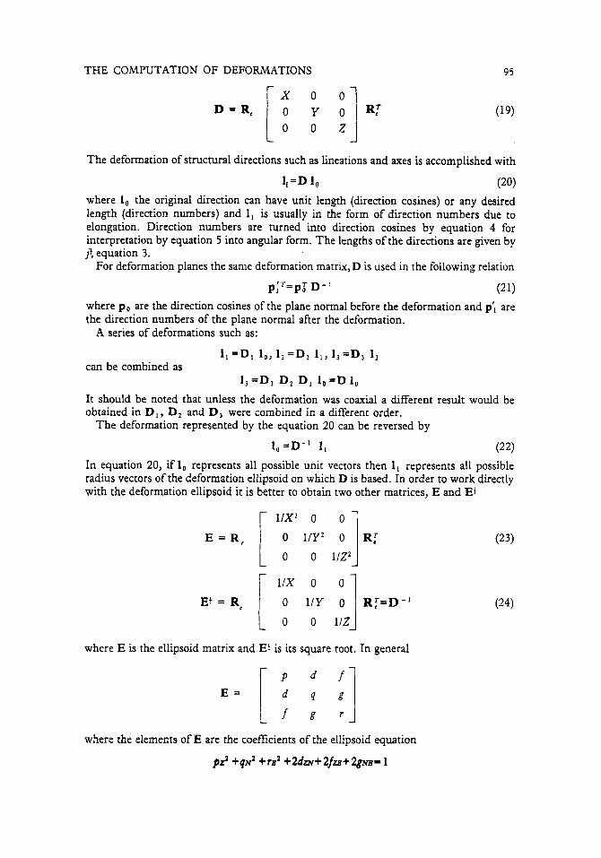
The deformation of structural directions such as lineations and axes is accomplished with

l ,=D 1, (20) where 1, the original direction can have unit length (direction cosines) or any desired length (direction numbers) and 1, is usually in the form of direction numbers due to elongation. Direction numbers are turned into direction cosines by equation 4 for interpretation by equation 5 into angular form. The lengths of the directions are given by j! equation 3 .

For deformation planes the same deformation matrix, D is used in the following relation

piT=pb D- ' (21) where p, are the direction cosines of the plane normal before the deformation and p', are the direction numbers of the plane normal after the deformation.

A series of deformations such as:

1, =D, lo, 1, =D, l , , 1, =D, 1, can be combined as

1, =D1 D, D, lo = D 1, It should be noted that unless the deformation was coaxial a different result would be obtained in D,, D, and D, were combined in a different order.

The deformation represented by the equation 20 can be reversed by

1, OD-' 1, (22) In equation 20, if 1, represents all possible unit vectors then 1, represents all possible radius vectors of the deformation ellipsoid on which D is based. In order to work directly with the deformation ellipsoid it is better to obtain two other matrices, E and Et

where E is the ellipsoid matrix and Ei is its square root. In general

where the elements of E are the coefficients of the ellipsoid equation

pz' +qN' +YE' +2dZiV+2fa+2gNBR1

96 D. FLI”

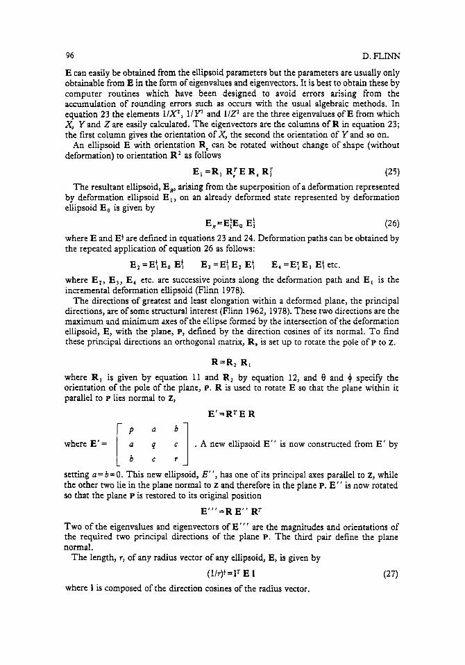
E can easily be obtained from the ellipsoid parameters but the parameters are usually only obtainable from E in the form of eigenvalues and eigenvectors. It is best to obtain these by computer routines which have been designed to avoid errors arising from the accumulation of rounding errors such as occurs with the usual algebraic methods. In equation 23 the elements 1/X2, l/P and l/Zz are the three eigenvalues of E from which X, Y and Z are easily calculated. The eigenvectors are the columns of R in equation 23; the first column gives the orientation of X, the second the orientation of Y and so on.

An ellipsoid E with orientation Re can be rotated without change of shape (without deformation) to orientation R2 as follows

E, = R , RITE R, R: (25 ) The resultant ellipsoid, E,, arising from the superposition of a deformation represented

by deformation ellipsoid E , , on an already deformed state represented by deformation ellipsoid E, is given by

E,=E~E, E! (26) where E and E+ are defined in equations 23 and 24. Deformation paths can be obtained by the repeated application of equation 26 as follows:

E2 =Et E, Ef E, =Et E, Efi where E,, E, , E, etc. are successive points along the deformation path and E , is the incremental deformation ellipsoid (Flinn 1978).

The directions of greatest and least elongation within a deformed plane, the principal directions, are of some structural interest (Flinn 1962, 1978). These two directions are the maximum and minimum axes of the ellipse formed by the intersection of the deformation ellipsoid, E, with the plane, p, defined by the direction cosines of its normal. T o find these principal directions an orthogonal matrix, R, is set up to rotate the pole of P to Z.

E, =Et E, Et etc.

R = R 2 R , where R , is given by equation 11 and R, by equation 12, and 8 and + specify the orientation of the pole of the plane, P. R is used to rotate E so that the plane within it parallel to P lies normal to Z,

E’=RrE R

. A new ellipsoid E” is now constructed from E’ by [: 9 :] where E’ =

setting a=b=O. This new ellipsoid, E“, has one of its principal axes parallel to Z, while the other two lie in the plane normal to Z and therefore in the plane P. E” is now rotated so that the plane P is restored to its original position

E”’=R E” RT

Two of the eigenvalues and eigenvectors of E”’ are the magnitudes and orientations of the required two principal directions of the plane P. The thrd pair define the plane normal.

The length, r, of any radius vector of any ellipsoid, E, is given by

(l/r)+=lT E 1 (27) where 1 is composed of the direction cosines of the radius vector.


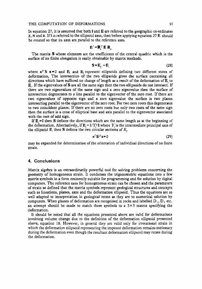
In equation 27, it is assumed that both 1 and E are referred to the geographic co-ordinates z, N and E. If I is referred to the ellipsoid axes, then before applying equation 27 E should be rotated so that its axes are parallel to the reference axes.

E’=R:E Rt The matrix S whose elements are the coefkients of the central quadric which is the

surface of no finite elongation is easily obtainable by matrix methods.

S=E, -Ei (28) where xT S x=O and E, and 5 represent ellipsoids defining two different states of deformation, The intersection of the two ellipsoids gives the surface containing all directions which have suffered no change of length as a result of the deformation of Ei to Ei. If the eigenvalues of S are all the same sign then the two ellipsoids do not intersect. If there are two eigenvalues of the same sign and a zero eigenvalue then the surface of intersection degenerates to a line parallel to the eigenvector of the zero root. If there are two eigenvalues of opposite sign and a zero eigenvalue the surface is two planes intersecting parallel to the eigenvector of the zero root. For two zero roots this degenerates to two coincident planes. If there are no zero roots but only two roots of the same sign then the surface is a cone of elliptical base and axis parallel to the eigenvector associated with the root of add sign.

If Ei=I then S defines the directions which are the same length as at the beginning of the deformation. Alternatively, if Ei = 1/ y+ I where Y is the intermediate principal axis of the ellipsoid Ei then S defines the two circular sections of Ei.

rTSTx=O (29) may be expanded for determination of the orientation of individual directions of no finite strain.

4. Conclusions

Matrix algebra is an extraordinarily powerhl tool for solving problems concerning the geometry of homogeneous strain. It condenses the trigonometric equations into a few matrix symbols in a form eminently suitable for programming and for solution by digital computers. The reference axes for homogeneous strain can be chosen and the parameters of strain so defined that the matrix symbols represent geological structures and concepts such as lineations, planes, axes and the deformation ellipsoid. Thus the equations are as well adapted to interpretation in geological terms as they are to numerical solution by computers. When phases of deformation are recognised in rocks and labelled D, , D, etc. an attempt should be made to match these symbols to a 3 x 3 matrix specifying the deformation.

It should be noted that all the equations presented above are valid for deformations involving volume change due to the definition of the deformation ellipsoid presented above, equation 18. However, in general they are valid only for irrotational strain in which the deformation ellipsoid representing the imposed deformation remains stationary during the deformation even though the resultant deformation ellipsoid may rotate during the deformation.

98 D. %INN

References

Flinn, I). 1962. On folding during three dimensional progressive deformation. Q. ?I. geul. Sue. Lond. 118,

-- 1978. Construction and computation of three-dimensional progressive deformations. Jl. geul. Suc.

Noble, B. 1969. Applied linear algebra. Prentice Hall, Lond. 522 pp. Phillips, P. C. 1960. The use of the stemgraphic projection in structural ~ m l o ~ . 2nd ed. Amold, Ldn. Schmidt, W. 1925. Gefuge statistik: Zeirschr. Min. 38, 392-423. Thompson, E. H. 1989. An introduction to the algebra of matriccs with some applications. A. Hiiger, tdn.

385-433.

Lund. 135, 291-305.

pp. 229.

Dept. of Geology University, Liverpool L69 38X

Documents

The computation of deformations