The Compton Effect-- Compton Scattering and … Compton Effect-- Compton Scattering and Gamma Ray Spectroscopy by Dr. James E. Parks Department of Physics and Astronomy 401 Nielsen

The Compton Effect-- Compton Scattering and Gamma Ray Spectroscopy

by Dr. James E. Parks

Department of Physics and Astronomy

401 Nielsen Physics Building The University of Tennessee

Knoxville, Tennessee 37996-1200

Revision 3.00 January 6, 2015 Copyright July 2004 & May 2014 by James Edgar Parks* *All rights are reserved. No part of this publication may be reproduced or transmitted in any form or by any means, electronic or mechanical, including photocopy, recording, or any information storage or retrieval system, without permission in writing from the author.

Objectives The objectives of this experiment are: (1) to study the interaction of high energy photons with matter, (2) to study photon-electron interactions (3) to study the photoelectric effect with high energy photons interacting with matter, (4) to study the effect of pair production and annihilation involving high energy photons, (5) to study the effects of backscatter and to learn about soft X-ray and Bremsstrahlung production, (6) to learn experimental techniques and procedures for measuring gamma-ray energy distributions, (7) to learn about photomultipliers and scintillation counters for measuring high energy photons, (8) to understand the operation, calibration, and use of a multichannel analyzer, (9) to learn data reduction and analysis techniques with measurements involving low signal to noise ratios, and (10) to learn to identify sources of background radiation and ways to minimize their effect. Introduction The Compton Effect is the quantum theory of the scattering of electromagnetic waves by a charged particle in which a portion of the energy of the electromagnetic wave is given to the charged particle in an elastic, relativistic collision. Compton scattering was discovered in 1922 by Arthur H. Compton (1892-1962) while conducting research on the scattering of X-rays by light elements. In 1922 he subsequently reported his experimental and theoretical results and received the Nobel prize in 1927 for this discovery. His theoretical explanation of what is now known as Compton scattering deviated from classical theory and required the use of special relativity and quantum mechanics, both of which were hardly understood at the time. When first reported, his

Compton Effect Page 2

results were controversial, but his work quickly triumphed and had a powerful effect on the future development of quantum theory. Compton scattering is the main focus of this experiment, but it is necessary to understand the interactions of high energy, electromagnetic photon radiation with materials in general. Gamma rays are high energy photons emitted from radioactive sources. When they interact with matter, there are three primary ways their energies can be absorbed by materials. These are the photoelectric effect, Compton scattering, and pair production. In addition to these primary processes, there are several lesser ways such as X-ray production and Bremsstrahlung. The Compton Effect is studied with the measurement of a gamma ray energy spectrum using a scintillator, photomultiplier tube, and multichannel analyzer. The gamma rays interact with the scintillator producing all three primary interaction processes so that the very phenomenon that is being studied in a sample is also taking place in the detector itself along with several other effects that mask the process of interest. References: 1. Arthur H. Compton, "A Quantum Theory of the Scattering of X-rays by Light Elements," The Physical Review, Vol. 21, No. 5, (May, 1923). Theory Compton scattering involves the scattering of photons by charged particles where both energy and momentum are transferred to the charged particle while the photon moves off with a reduced energy and a change of momentum. Generally, the charged particle is an electron considered to be at rest and the photon is usually considered to be an energetic photon such as an X-ray photon or gamma ray photon. In this experiment gamma rays from a cesium-137 source are used for the source of photons that are scattered and each photon has an energy of 0.662 MeV when incident on the target scatterer. The charged particle is assumed to be an electron at rest in the target. While the theory here is applied to gamma rays and electrons, the theory works just as well for less energetic photons such as found in visible light and other particles. The theory of Compton scattering uses relativistic mechanics for two reasons. First, it involves the scattering of photons that are massless, and secondly, the energy transferred to the electron is comparable to its rest energy. As a result the energy and momentum of the photons and electrons must be expressed using their relativistic values. The laws of conservation of energy and conservation of momentum are then used with these relativistic values to develop the theory of Compton scattering. From the special theory of relativity, an object whose rest mass is 0m and is moving at a

velocity v will have a relativistic mass m given by


0

2

1

mm

vc

(1)

The relativistic momentum p

is defined as mv

so that squaring both sides of Equation

(1) and multiplying by 4c leads to

22 2 2

0 vm m mc ,

2 4 2 2 2 2 4

0 m c m v c m c ,

2 222 20 mc pc m c ,

22 20 E pc E ,

and

2 2 20pc E E . (2)

Equation (2) then relates the magnitude of the relativistic momentum p

of an object to its

relativistic energy E and its rest energy 0E . From this equation it is readily seen that the

magnitudes of momentum and energy of a massless particle such as a photon are related by

pc E . (3) or

E h h

pc c

. (4)

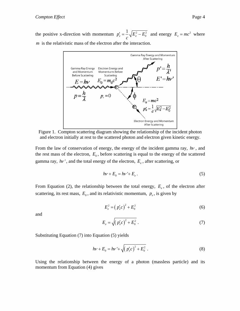
Figure 1 illustrates the scattering of an incident photon of energy E h moving to the

right in the positive x direction with a momentum h h

pc

and interacting with an

electron at rest with momentum 0ep and energy equal to its rest energy, 20 0E m c .

The symbols, h , , and , are the standard symbols used for Planck's constant, the photon's frequency, and its wavelength. 0m is the rest mass of the electron. In the

interaction, the gamma ray is scattered in the positive x and y directions at an angle

with momentum of magnitude '

''

h hp

c

and energy ' 'E h . The electron is

scattered in the positive x-direction and negative y-direction at an angle with respect to


the positive x-direction with momentum 2 20

1e ep E E

c and energy 2

eE mc where

m is the relativistic mass of the electron after the interaction.

Figure 1. Compton scattering diagram showing the relationship of the incident photon and electron initially at rest to the scattered photon and electron given kinetic energy.

From the law of conservation of energy, the energy of the incident gamma ray, h , and the rest mass of the electron, 0E , before scattering is equal to the energy of the scattered

gamma ray, 'h , and the total energy of the electron, eE , after scattering, or

0 ' eh E h E . (5)

From Equation (2), the relationship between the total energy, eE , of the electron after

scattering, its rest mass, 0E , and its relativistic momentum, ep , is given by

22 20e eE p c E (6)

and

2 20e eE p c E . (7)

Substituting Equation (7) into Equation (5) yields

2 20 0' eh E h p c E . (8)

Using the relationship between the energy of a photon (massless particle) and its momentum from Equation (4) gives


2 20 0epc E p c p c E . (9)

Rearranging gives

2 20 0ep p c E p c E (10)

and

2 22 2 20 0 02 ep p c E p p cE p c E (11)

that results in the following expression based on conservation of energy

02 2 22

2 e

p p Ep p pp p

c

. (12)

Equation (12) is then an expression relating the momentum ep of the electron given to it

by a scattered gamma ray whose initial momentum was p and whose final momentum is 'p . The electron was assumed to be initially at rest and it was also assumed to be given

enough energy for relativistic mechanics to apply. Equation (12) is solely based on the law of conservation of energy, but another independent expression for the momentum ep

can be found based on the law of conservation of momentum. In the scattering process momentum must be conserved so that Total Momentum Before = Total Momentum After . (13) Since momentum is a vector quantity, Total Momentum in X-Direction Before = Total Momentum in X-Direction After (14) and Total Momentum in Y-Direction Before = Total Momentum in Y-Direction After . (15) For an electron at rest, its initial momentum is zero and has no x and y components. For an incident gamma ray photon moving in the positive x direction and interacting with an electron at rest, the initial x-component of momentum is p and the y-component is zero so that ' cos cosep p p (16)

and 0 'sin ( ) sinep p (17)


where 'p and ep are the momenta of the scattered gamma ray and electron after

interacting. Rearranging Equations (16) and (17) and squaring both sides of each produces cos 'cosep p p , (18)

sin 'sinep p , (19)

2 2 2 2 2cos ' cos 2 'cosep p p pp , (20)

and 2 2 2 2sin ' sinep p . (21)

Adding Equations (20) and (21) yields

2 2 2 2 2 2 2sin cos ' sin cos 2 'cosep p p pp (22)

That can be simplified using the indentity 2 2cos sin 1x x to further yield 2 2 2' 2 'cosep p p pp . (23)

Equation (23) is then an expression based on the law of conservation of momentum that relates the momentum given to the electron from its rest position by the incident gamma ray of momentum p interacting with the electron so that it is scattered off at angle with momentum 'p . Equating Equations (12) and (23), one based on conservation of energy and the other on conservation of momentum, gives

02 2 2 22

2 ' 2 'cosp p E

p p pp p p ppc

(24)

that reduces to

02

2 2 'cosp p E

pp ppc

, (25)

and

0

1 11 cos

'

c

p p E . (26)

Using the relationships for momentum, energy, wavelength, and frequency for photons,

h h Ep

c c

, Equation (26) can be transformed into


0

1 1 11 cos

'E E E (27)

that relates the energy of a scattered photon 'E to the energy of the incident photon E and the scattering angle . Equation (27) is a simple equation that can be used to verify the theory for the Compton Effect. The energy of incident gamma rays E can be easily measured with a scintillator-photomutiplier detector and multichannel analyzer system. The energy of the scattered gamma rays 'E as a function of can also be easily measured with the same system. A

plot of measurements of 1 1

'E E versus measurements of 1 cos should result in a

linear graph whose slope is the inverse of the electron’s rest energy 0

1

E.

Gamma Ray Spectroscopy and the Scintillation Detector Data to verify the Compton Scattering theory is collected in this experiment using a gamma ray spectrometer that consists of a scintillation detector, high voltage supply, amplifier system, and a multichannel analyzer to measure the energy distribution of the detected gamma rays. There are many ways to detect gamma rays, and these include: ionization chambers, photographic film, proportional counters, Geiger-Mueller detectors, solid state diodes, germanium detectors, liquid and solid scintillation materials with photomultiplier tubes, and a number of methods using similar materials and approaches. To study the Compton Effect a gamma ray spectroscopy method is needed to measure the gamma ray’s energy before and after an interaction. A scintillation detector is capable of doing this, and the one used in this experiment is composed of a sodium iodide (NaI) scintillation crystal and a photomultiplier tube. The detector system produces a voltage pulse that is proportional to the energy deposited in the crystal by the absorbed gamma ray. The detected gamma ray may be from the radioactive source either directly or by scattering. The size of the voltage pulse, and hence the energy deposited in the detector, is measured with a multichannel analyzer (MCA). The energy deposited in the scintillation crystal depends on the type of interaction between the gamma ray and the crystal even for a single gamma ray of a single energy. An MCA measures the distribution of voltage pulse heights, or spectrum of voltage pulses, for multiple gamma rays interacting in the crystal depending on the type of interaction that occurs. When a gamma ray interacts with matter, there are interactions that occur in the material other than those due to the Compton scattering. All of these interactions occur in the detector just like they occur in the material that the effect is being studied. There are 3 primary ways that gamma rays interact with matter, and these are: (1) photoelectric absorption, (2) Compton scattering, and (3) pair production. In addition to these 3 primary ones, there are other effects such as X-ray production. All of these effects occur in the detector, just as they do in the material that is being studied and they make up


different portions of the measured energy spectra. Photoelectric absorption predominates for low-energy gamma rays (up to several hundred keV), pair production predominates for high-energy gamma rays (above 5-10 MeV), and Compton scattering is the most probable process over the range of energies between these extremes. Of the three types of interactions, photoelectric absorption is the most significant mechanism for making practical energy measurements of low energy gamma rays in an energy range up to several hundred keV, the range of gamma ray energies to be measured in this experiment. In the photoelectric effect, the energy of a photon is transferred to the electron by first supplying enough energy to release it from its bound state to a nucleus and then transferring the rest of its energy into kinetic energy of the freed electron. Typically, the electron that is ejected is a K shell electron whose binding energy is a few keV. This is relatively a small amount compared to the energy of the gamma ray so that most of the incident energy is then transferred to kinetic energy of the electron. Therefore, if the energy of the gamma ray is E , its energy will be first transferred to the

binding energy bE of the electron to free it from its nucleus and then the remainder of its

energy will be transferred to the electron’s kinetic energy e

E or

be

E E E . (28)

The kinetic energy of the electron is then given by be

E E E . (29)

In this experiment 0.662 MeV ( 662 keVE ) gamma rays are emitted from the

radioactive source. If the binding energy of the electron in the scintillator is a few keV, take 2 keVbE for an example, then an electron ejected by the photoelectric effect

would typically have an energy 660 keVe

E , nearly equal to the energy of the gamma

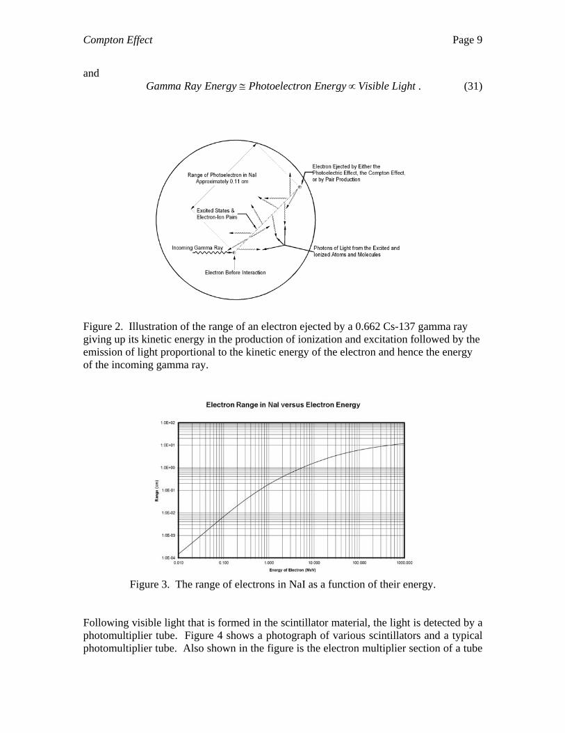
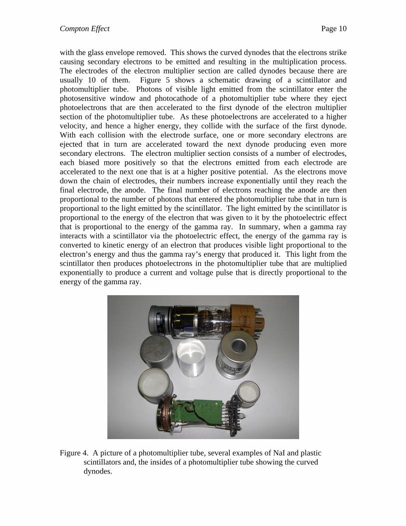
ray (within 0.3%). The photoelectric absorption process then converts electromagnetic energy of a gamma ray photon into kinetic energy of a charged particle, an electron. As illustrated in Figure 2, the kinetic energy of an electron is dissipated in a very short distance by elastic and inelastic collisions with the material in which the photoelectron was created. The range of a 0.662 MeV electron in NaI is about 1 millimeter (specifically 0.111 cm), and gives up its energy by creating ionization and excitation along its path. (See graph in Figure 3 that shows the range of electrons in NaI as a function of their energy.) Photons of visible light are produced along the electron’s path as the excited states give up their energy by de-excitation back to their normal, ground state condition. The amount of light that is produced is proportional to the energy of the photoelectron which in turn is nearly equal to the energy of the gamma ray that produced it. In other words, Gamma Ray Energy Photoelectron Energy Visible Light (30)


and Gamma Ray Energy Photoelectron Energy Visible Light . (31)

Figure 2. Illustration of the range of an electron ejected by a 0.662 Cs-137 gamma ray giving up its kinetic energy in the production of ionization and excitation followed by the emission of light proportional to the kinetic energy of the electron and hence the energy of the incoming gamma ray.

Figure 3. The range of electrons in NaI as a function of their energy.

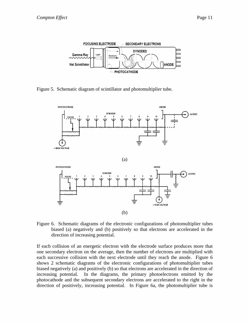
Following visible light that is formed in the scintillator material, the light is detected by a photomultiplier tube. Figure 4 shows a photograph of various scintillators and a typical photomultiplier tube. Also shown in the figure is the electron multiplier section of a tube


with the glass envelope removed. This shows the curved dynodes that the electrons strike causing secondary electrons to be emitted and resulting in the multiplication process. The electrodes of the electron multiplier section are called dynodes because there are usually 10 of them. Figure 5 shows a schematic drawing of a scintillator and photomultiplier tube. Photons of visible light emitted from the scintillator enter the photosensitive window and photocathode of a photomultiplier tube where they eject photoelectrons that are then accelerated to the first dynode of the electron multiplier section of the photomultiplier tube. As these photoelectrons are accelerated to a higher velocity, and hence a higher energy, they collide with the surface of the first dynode. With each collision with the electrode surface, one or more secondary electrons are ejected that in turn are accelerated toward the next dynode producing even more secondary electrons. The electron multiplier section consists of a number of electrodes, each biased more positively so that the electrons emitted from each electrode are accelerated to the next one that is at a higher positive potential. As the electrons move down the chain of electrodes, their numbers increase exponentially until they reach the final electrode, the anode. The final number of electrons reaching the anode are then proportional to the number of photons that entered the photomultiplier tube that in turn is proportional to the light emitted by the scintillator. The light emitted by the scintillator is proportional to the energy of the electron that was given to it by the photoelectric effect that is proportional to the energy of the gamma ray. In summary, when a gamma ray interacts with a scintillator via the photoelectric effect, the energy of the gamma ray is converted to kinetic energy of an electron that produces visible light proportional to the electron’s energy and thus the gamma ray’s energy that produced it. This light from the scintillator then produces photoelectrons in the photomultiplier tube that are multiplied exponentially to produce a current and voltage pulse that is directly proportional to the energy of the gamma ray.

Figure 4. A picture of a photomultiplier tube, several examples of NaI and plastic

scintillators and, the insides of a photomultiplier tube showing the curved dynodes.


Figure 5. Schematic diagram of scintillator and photomultiplier tube.

(a)

(b)

Figure 6. Schematic diagrams of the electronic configurations of photomultiplier tubes

biased (a) negatively and (b) positively so that electrons are accelerated in the direction of increasing potential.

If each collision of an energetic electron with the electrode surface produces more that one secondary electron on the average, then the number of electrons are multiplied with each successive collision with the next electrode until they reach the anode. Figure 6 shows 2 schematic diagrams of the electronic configurations of photomultiplier tubes biased negatively (a) and positively (b) so that electrons are accelerated in the direction of increasing potential. In the diagrams, the primary photoelectrons emitted by the photocathode and the subsequent secondary electrons are accelerated to the right in the direction of positively, increasing potential. In Figure 6a, the photomultiplier tube is


biased negatively with negative high voltage to the photocathode itself and with the anode at ground potential. A series resistor string biases each successive electrode less negatively (more positively) until ground (zero) potential is reached at the anode. The multiplied electrons are collected at the anode and are returned to ground through a resistor, thus producing a voltage pulse for each gamma ray detected in the scintillator. The advantage to this arrangement is the signal is taken near ground, removing sensitive amplifier inputs from the high voltage, freeing it from induced noise due to high voltage fluctuations, and being safer for the operator. It also has the advantage of allowing the direct collection of the electron current that is particularly useful for detection of constant light sources. The arrangement in Figure 6b sets the ground potential at the photocathode and biases the anode with a positive high voltage. Having the photocathode at ground potential avoids potential problems of spurious emissions from the photocathode due to high voltage that are greatly magnified as the signal is multiplied as it proceeds down the string of electrodes. Since the anode is at a high potential, it must be isolated from amplifier inputs to avoid destroying amplifier components. A blocking capacitor is used to isolate the high voltage from the output of the circuit and the amplifier input. For the detection of gamma rays that occur mostly as single events spaced apart in time, this is no problem. Each detected gamma ray produces a pulse of electrons to the anode that in turn produces a voltage pulse across the load resistor. The voltage pulse is easily transmitted through the blocking capacitor to the circuit’s output.

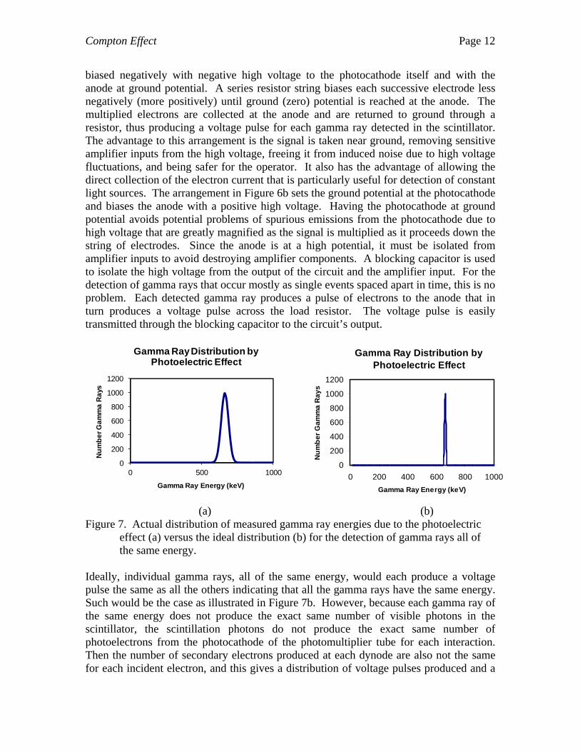
(a) (b) Figure 7. Actual distribution of measured gamma ray energies due to the photoelectric

effect (a) versus the ideal distribution (b) for the detection of gamma rays all of the same energy.

Ideally, individual gamma rays, all of the same energy, would each produce a voltage pulse the same as all the others indicating that all the gamma rays have the same energy. Such would be the case as illustrated in Figure 7b. However, because each gamma ray of the same energy does not produce the exact same number of visible photons in the scintillator, the scintillation photons do not produce the exact same number of photoelectrons from the photocathode of the photomultiplier tube for each interaction. Then the number of secondary electrons produced at each dynode are also not the same for each incident electron, and this gives a distribution of voltage pulses produced and a

0

200

400

600

800

1000

1200

0 500 1000

Nu

mb

er

Ga

mm

a R

ays

Gamma Ray Energy (keV)

Gamma Ray Distribution by Photoelectric Effect

Gamma Ray Distribution by Photoelectric Effect

0

200

400

600

800

1000

1200

0 200 400 600 800 1000

Gamma Ray Energy (keV)

Nu

mb

er

Ga

mm

a R

ay

s


distribution of energies measured. The distribution for single energy gamma rays is then a Gaussian distribution much like that shown in Figure 7a. Photoelectrons emitted near the edges in the scintillator can lose a portion or all of their energy to the walls of the scintillator’s enclosure thus producing a lesser voltage pulse in the detector. The second most important way a gamma ray interacts with a scintillation detector is by the Compton Effect, the subject of this experiment. The very phenomena that is being studied and measured is an important process that takes place in the detector that is being used to study the same process in another material. Just as a gamma ray can transfer its energy to an electron in a scintillator material by the photoelectric effect, it can also transfer a portion of its energy to an electron by the Compton Effect. Whereas the transfer of gamma ray energy to an electron via the photoelectric effect is always nearly 100%, the transfer of energy via the Compton Effect can range from 0% to nearly 100%, depending on the energy of the gamma ray and the angle that it is scattered. Recalling Equation (27) with 2

0 0E m c ,

20

1 1 11 cos

'E E m c (32)

and applying the law of conservation of energy, the energy given to an electron by Compton Scattering is

20

20

20

1' 1

1 cos 1 1 cose

E m cE E E E E

Em c Em c

. (33)

Since the maximum kinetic energy transferred to the electron is for 180 , the maximum energy transferred is given by

20

1' 1

1 2eMaxE E E E

Em c

. (34)

For values of 2E mc , the maximum energy that can be transferred to the electron is nearly equal to the energy of the gamma ray, and eMaxE E . For values of 2E mc , the

maximum energy that can be transferred to the electron is approximately zero or, 0eMaxE . The percentage of the maximum of the gamma ray’s initial energy that is

transferred to the electron in Compton scattering is about 72% for a 0.662 MeV gamma ray. Therefore, Compton scattering with 0.662 MeV gamma rays will give scattered electrons energies ranging from 0 to 0.477 MeV.


The probability of gamma rays scattering at a particular angle and imparting an energy

eE to the electron can be calculated from the Klein-Nashina equation for unpolarized

rays given by

2

2 2102

' 'sin

'

E E Ed r d

E E E

, (35)

where d is the differential cross section for scattering as a function of the scattering

angle , 'E

E is the ratio the gamma ray’s energy before and after scattering, 0r is the

classical radius of the electron, and d is the differential solid angle. From symmetry, since sind d d , Equation (35) may be integrated over to yield

2

2 2102

' 'sin 2 sin

'

E E Ed r d

E E E

(36)

or

202 sin

dr g

d

(37)

where

2

212

' 'sin

'

E E Eg

E E E

. (38)

Using Equation (33) for the energy imparted to the electron by Compton scattering and the Klein-Nashina equation for the angular probability function, the energy probability as

a function of the electron energy, e

d

dE

may be found by using the chain rule,

1

e

e e

dEd d d d

dE d dE d d

. (39)

Differentiating eE given by Equation (33) with respect to gives the inverse of e

d

dE

,

1

edE

d

, so that given

2

0

11

1 1 coseE E

Em c

, (40)


2

2 20 0

1 1 1 cos sinedE dE E EE

d d m c m c

, (41)

2 2

0

20

sin

1 1 cos

edE E E

d m cEm c

, (42)

and

2

21 02

02

1 1 cos

sine

Em c

m cdE

d E

. (43)

Inserting the expressions for d

d

and 1

edE

d

given by Equations (37) and (43)

respectively,

2

202

020 2

1 1 cos

2 sinsine

Em c

m cdr g

dE E

. (44)

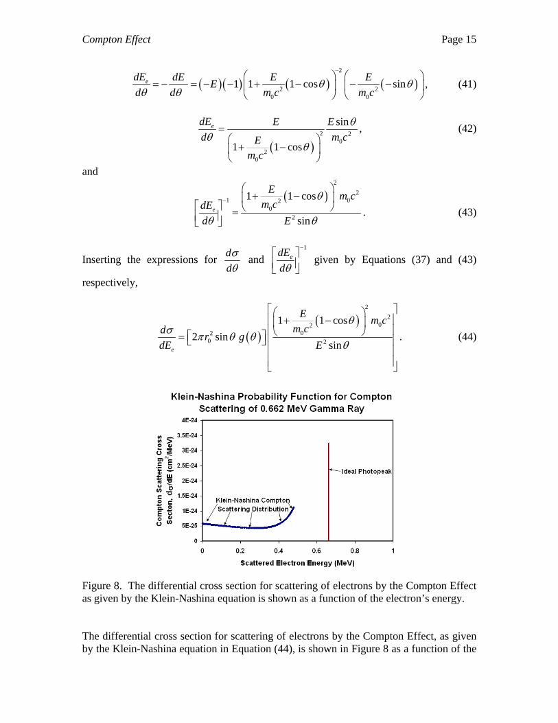
Figure 8. The differential cross section for scattering of electrons by the Compton Effect as given by the Klein-Nashina equation is shown as a function of the electron’s energy. The differential cross section for scattering of electrons by the Compton Effect, as given by the Klein-Nashina equation in Equation (44), is shown in Figure 8 as a function of the


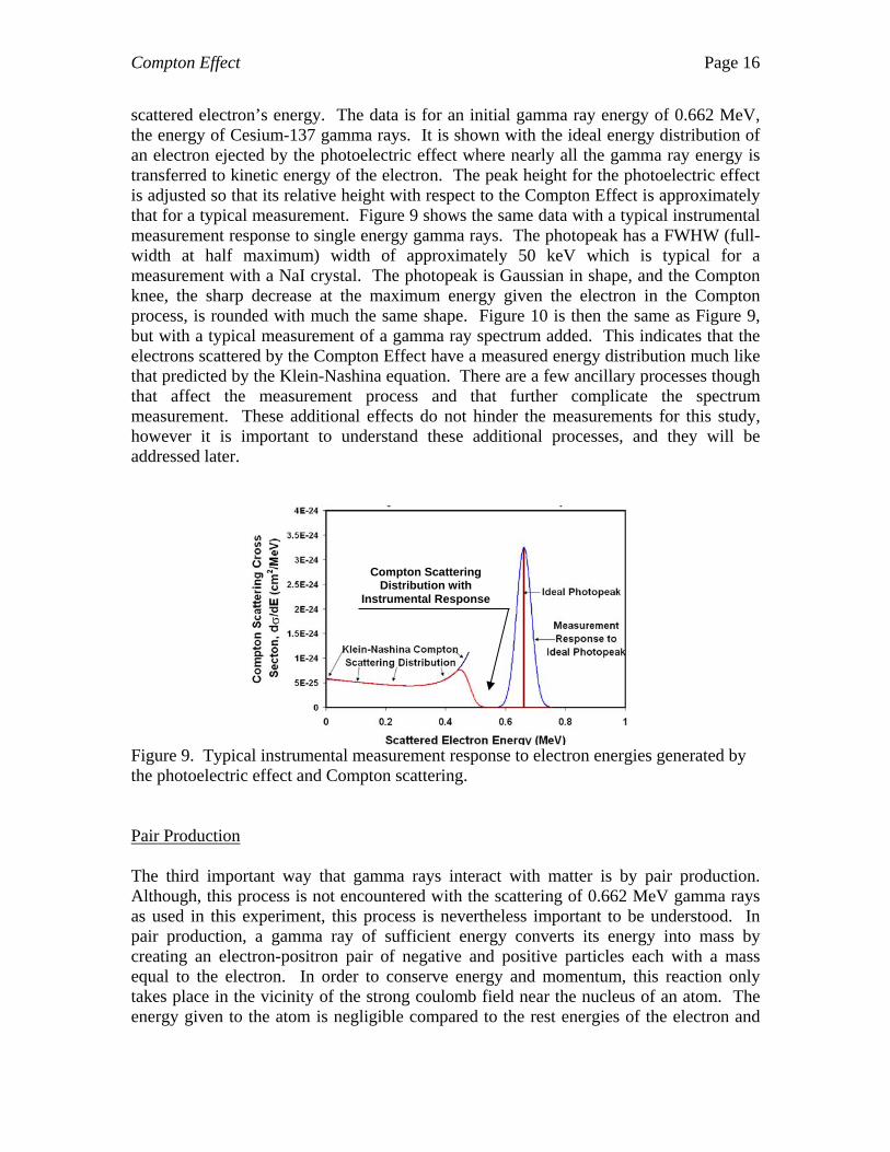
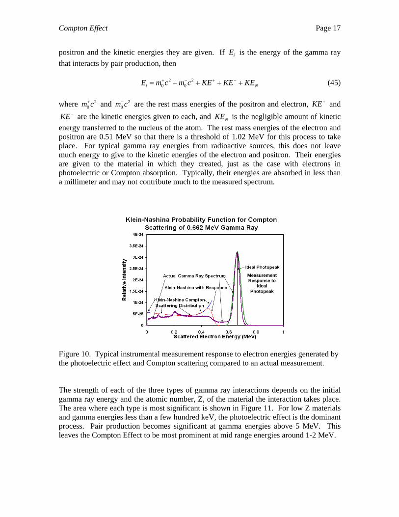
scattered electron’s energy. The data is for an initial gamma ray energy of 0.662 MeV, the energy of Cesium-137 gamma rays. It is shown with the ideal energy distribution of an electron ejected by the photoelectric effect where nearly all the gamma ray energy is transferred to kinetic energy of the electron. The peak height for the photoelectric effect is adjusted so that its relative height with respect to the Compton Effect is approximately that for a typical measurement. Figure 9 shows the same data with a typical instrumental measurement response to single energy gamma rays. The photopeak has a FWHW (full-width at half maximum) width of approximately 50 keV which is typical for a measurement with a NaI crystal. The photopeak is Gaussian in shape, and the Compton knee, the sharp decrease at the maximum energy given the electron in the Compton process, is rounded with much the same shape. Figure 10 is then the same as Figure 9, but with a typical measurement of a gamma ray spectrum added. This indicates that the electrons scattered by the Compton Effect have a measured energy distribution much like that predicted by the Klein-Nashina equation. There are a few ancillary processes though that affect the measurement process and that further complicate the spectrum measurement. These additional effects do not hinder the measurements for this study, however it is important to understand these additional processes, and they will be addressed later.

Figure 9. Typical instrumental measurement response to electron energies generated by the photoelectric effect and Compton scattering. Pair Production The third important way that gamma rays interact with matter is by pair production. Although, this process is not encountered with the scattering of 0.662 MeV gamma rays as used in this experiment, this process is nevertheless important to be understood. In pair production, a gamma ray of sufficient energy converts its energy into mass by creating an electron-positron pair of negative and positive particles each with a mass equal to the electron. In order to conserve energy and momentum, this reaction only takes place in the vicinity of the strong coulomb field near the nucleus of an atom. The energy given to the atom is negligible compared to the rest energies of the electron and

Compton Scattering Distribution with

Instrumental Response


positron and the kinetic energies they are given. If iE is the energy of the gamma ray

that interacts by pair production, then 2 2

0 0i NE m c m c KE KE KE (45)

where 2

0m c and 20m c are the rest mass energies of the positron and electron, KE and

KE are the kinetic energies given to each, and NKE is the negligible amount of kinetic

energy transferred to the nucleus of the atom. The rest mass energies of the electron and positron are 0.51 MeV so that there is a threshold of 1.02 MeV for this process to take place. For typical gamma ray energies from radioactive sources, this does not leave much energy to give to the kinetic energies of the electron and positron. Their energies are given to the material in which they created, just as the case with electrons in photoelectric or Compton absorption. Typically, their energies are absorbed in less than a millimeter and may not contribute much to the measured spectrum.

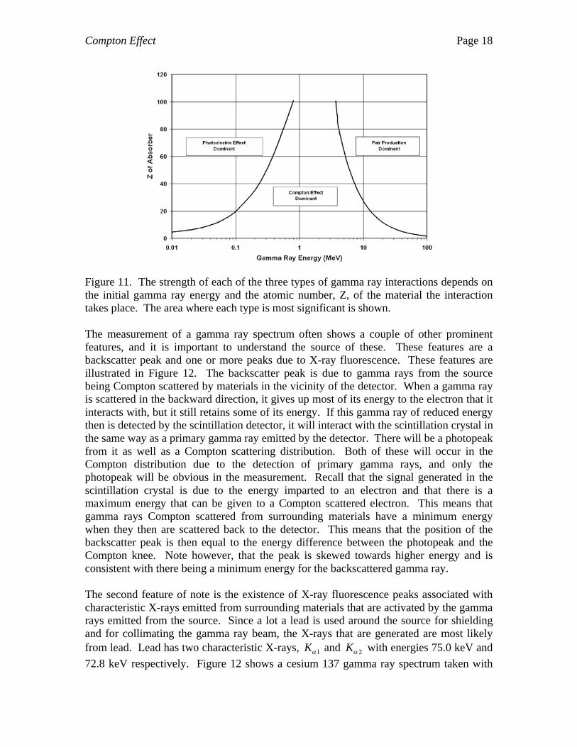
Figure 10. Typical instrumental measurement response to electron energies generated by the photoelectric effect and Compton scattering compared to an actual measurement. The strength of each of the three types of gamma ray interactions depends on the initial gamma ray energy and the atomic number, Z, of the material the interaction takes place. The area where each type is most significant is shown in Figure 11. For low Z materials and gamma energies less than a few hundred keV, the photoelectric effect is the dominant process. Pair production becomes significant at gamma energies above 5 MeV. This leaves the Compton Effect to be most prominent at mid range energies around 1-2 MeV.

Measurement Response to

Ideal Photopeak


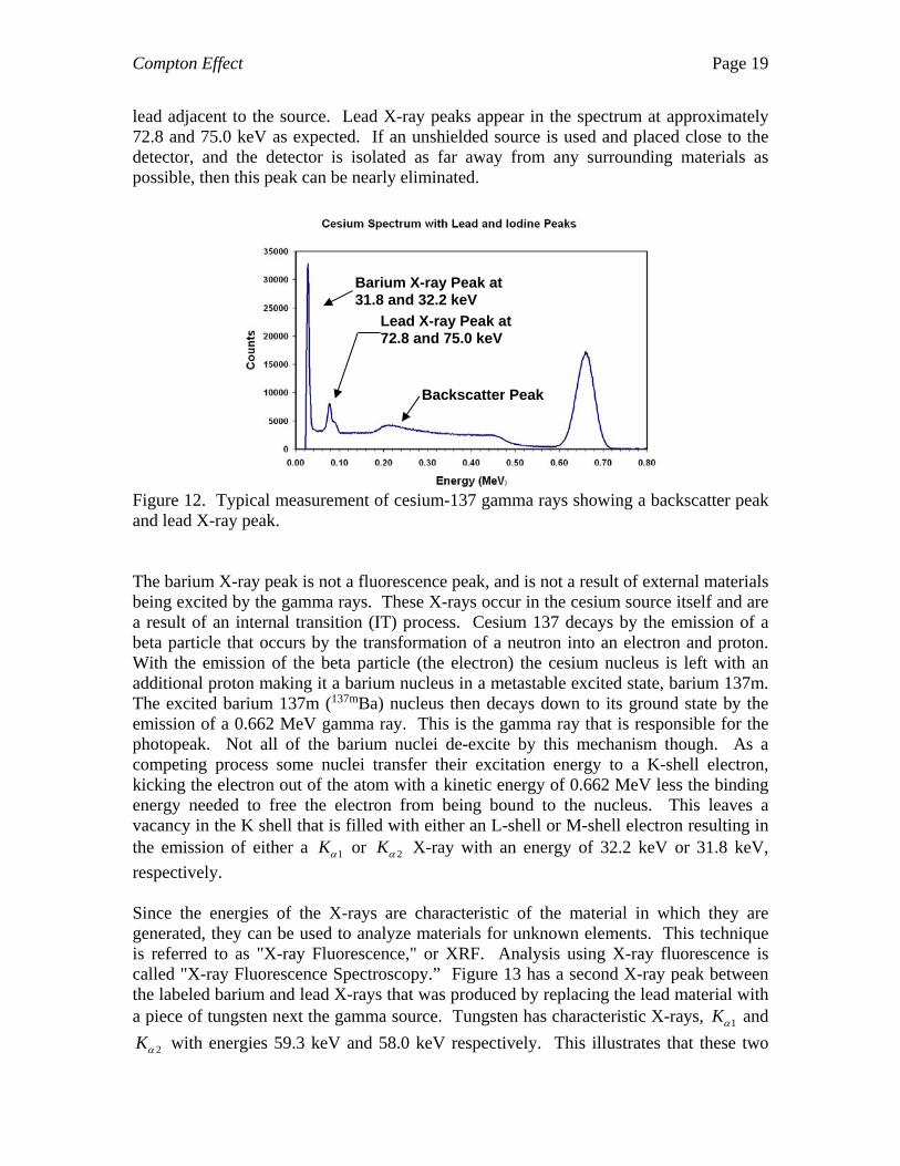
Figure 11. The strength of each of the three types of gamma ray interactions depends on the initial gamma ray energy and the atomic number, Z, of the material the interaction takes place. The area where each type is most significant is shown. The measurement of a gamma ray spectrum often shows a couple of other prominent features, and it is important to understand the source of these. These features are a backscatter peak and one or more peaks due to X-ray fluorescence. These features are illustrated in Figure 12. The backscatter peak is due to gamma rays from the source being Compton scattered by materials in the vicinity of the detector. When a gamma ray is scattered in the backward direction, it gives up most of its energy to the electron that it interacts with, but it still retains some of its energy. If this gamma ray of reduced energy then is detected by the scintillation detector, it will interact with the scintillation crystal in the same way as a primary gamma ray emitted by the detector. There will be a photopeak from it as well as a Compton scattering distribution. Both of these will occur in the Compton distribution due to the detection of primary gamma rays, and only the photopeak will be obvious in the measurement. Recall that the signal generated in the scintillation crystal is due to the energy imparted to an electron and that there is a maximum energy that can be given to a Compton scattered electron. This means that gamma rays Compton scattered from surrounding materials have a minimum energy when they then are scattered back to the detector. This means that the position of the backscatter peak is then equal to the energy difference between the photopeak and the Compton knee. Note however, that the peak is skewed towards higher energy and is consistent with there being a minimum energy for the backscattered gamma ray. The second feature of note is the existence of X-ray fluorescence peaks associated with characteristic X-rays emitted from surrounding materials that are activated by the gamma rays emitted from the source. Since a lot a lead is used around the source for shielding and for collimating the gamma ray beam, the X-rays that are generated are most likely from lead. Lead has two characteristic X-rays, 1K and 2K with energies 75.0 keV and

72.8 keV respectively. Figure 12 shows a cesium 137 gamma ray spectrum taken with


lead adjacent to the source. Lead X-ray peaks appear in the spectrum at approximately 72.8 and 75.0 keV as expected. If an unshielded source is used and placed close to the detector, and the detector is isolated as far away from any surrounding materials as possible, then this peak can be nearly eliminated.

Figure 12. Typical measurement of cesium-137 gamma rays showing a backscatter peak and lead X-ray peak.

The barium X-ray peak is not a fluorescence peak, and is not a result of external materials being excited by the gamma rays. These X-rays occur in the cesium source itself and are a result of an internal transition (IT) process. Cesium 137 decays by the emission of a beta particle that occurs by the transformation of a neutron into an electron and proton. With the emission of the beta particle (the electron) the cesium nucleus is left with an additional proton making it a barium nucleus in a metastable excited state, barium 137m. The excited barium 137m (137mBa) nucleus then decays down to its ground state by the emission of a 0.662 MeV gamma ray. This is the gamma ray that is responsible for the photopeak. Not all of the barium nuclei de-excite by this mechanism though. As a competing process some nuclei transfer their excitation energy to a K-shell electron, kicking the electron out of the atom with a kinetic energy of 0.662 MeV less the binding energy needed to free the electron from being bound to the nucleus. This leaves a vacancy in the K shell that is filled with either an L-shell or M-shell electron resulting in the emission of either a 1K or 2K X-ray with an energy of 32.2 keV or 31.8 keV,

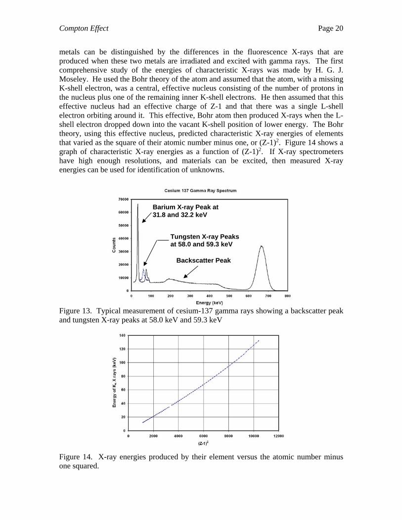
respectively. Since the energies of the X-rays are characteristic of the material in which they are generated, they can be used to analyze materials for unknown elements. This technique is referred to as "X-ray Fluorescence," or XRF. Analysis using X-ray fluorescence is called "X-ray Fluorescence Spectroscopy.” Figure 13 has a second X-ray peak between the labeled barium and lead X-rays that was produced by replacing the lead material with a piece of tungsten next the gamma source. Tungsten has characteristic X-rays, 1K and

2K with energies 59.3 keV and 58.0 keV respectively. This illustrates that these two

Barium X-ray Peak at 31.8 and 32.2 keV

Lead X-ray Peak at 72.8 and 75.0 keV

Backscatter Peak


metals can be distinguished by the differences in the fluorescence X-rays that are produced when these two metals are irradiated and excited with gamma rays. The first comprehensive study of the energies of characteristic X-rays was made by H. G. J. Moseley. He used the Bohr theory of the atom and assumed that the atom, with a missing K-shell electron, was a central, effective nucleus consisting of the number of protons in the nucleus plus one of the remaining inner K-shell electrons. He then assumed that this effective nucleus had an effective charge of Z-1 and that there was a single L-shell electron orbiting around it. This effective, Bohr atom then produced X-rays when the L-shell electron dropped down into the vacant K-shell position of lower energy. The Bohr theory, using this effective nucleus, predicted characteristic X-ray energies of elements that varied as the square of their atomic number minus one, or (Z-1)2. Figure 14 shows a graph of characteristic X-ray energies as a function of (Z-1)2. If X-ray spectrometers have high enough resolutions, and materials can be excited, then measured X-ray energies can be used for identification of unknowns.

Figure 13. Typical measurement of cesium-137 gamma rays showing a backscatter peak and tungsten X-ray peaks at 58.0 keV and 59.3 keV

Figure 14. X-ray energies produced by their element versus the atomic number minus one squared.

Backscatter Peak

Tungsten X-ray Peaks at 58.0 and 59.3 keV

Barium X-ray Peak at 31.8 and 32.2 keV


Apparatus

The apparatus is shown in Figures 15 and 17 and consists of: (1) a 30 millicurie cesium source located in a shielded lead housing that also collimates the beam of gamma rays emanating from it, (2) a detector system consisting of a sodium iodide scintillation crystal, photomultiplier tube, and pre-amplifier, (3) a lead shield for the detector to allow only gamma rays to enter the crystal from the scatterer at a small angle, (4) a scattering sample consisting of either an aluminum or plastic cylinder, (5) a goniometer to orient the detector system at various scattering angles with respect to the collimated beam of incident gamma rays and scatterer, (6) a multichannel analyzer system consisting of a Spectrum Techniques Model UCS-30 Universal Computer Spectrometer with software program, and (7) a computer system with Microsoft Office.

Figure 15. Apparatus and setup for the Compton Effect experiment. The Multichannel Analyzer Setup and Calibration In gamma ray spectroscopy, a single gamma ray may interact in one or more different ways to produce a distribution of voltage pulses proportional to the energies deposited in the detector. These voltage pulses are primarily determined by the type of mechanism that the gamma ray interacts with the detector and/or the materials surrounding the detector. The voltage pulse depends not only on the type of interaction, but also on the high voltage of the photomultiplier tube, its efficiency, the efficiency of the scintillator,


the amplifier gain, and the interaction position in the scintillator relative to the edges where loss effects take place. All of these processes are subject to statistical fluctuations, but with stable electronics and repetitive measurements of the interactions, a true representation of the interaction distribution can be measured. A multichannel analyzer, MCA, is used to measure voltage distributions and hence the energy distributions of gamma interactions. An MCA is an electronic instrument that takes a voltage range, divides it into a number of increments or channels, measures an input voltage, and then assigns it to a channel based on its value being equal to or greater than the beginning value of the channel but less than its beginning value plus the incremental value. The number of pulses assigned to any one channel are counted and recorded and can be recalled to display the measured distribution of pulses as a function of the value of the pulses. For example, an MCA typically measures input pulses ranging from 0 to 10 volts, and this range is typically divided into 1024 channels, each representing an incremental range of 9.7656 mV. The 1024 channels are numbered 0 to 1023 starting with the first channel as “channel 0” to the last channel as “channel 1023.” Channel 409 records the total number of pulses whose input values are equal to or more than 3.994140625 volts but less that 4.00390625 volts. Therefore, a voltage pulse of 4 volts will be registered in channel 409. While MCAs are designed to be linear devices, this is not always the case. In addition, it is also assumed that scintillators and photomultiplier tubes are linear devices. Instead of the spectrometer system (MCA plus amplifiers and detector) being linear, it may have a small quadratic or higher power dependence. To a first approximation, a MCA system can be assumed to be linear and can be calibrated with only one known energy value. Two values are better, and three are even better for more precise calibrations. There are sets of radioactive sources, each with different gamma ray energies, that can be used as standards to calibrate the system. Using only one gamma ray energy forces the calibration to be linear and for the intercept of channel number versus energy to be zero, i.e. zero energy coincides with channel zero. Two gamma ray energies still forces the relationship between energy and channels to be linear, but zero energy may line up with some other channel other than channel zero. This two-point calibration is important in cases where there are zero offsets, or dc voltage offsets, in the electronic instrumentation. A three-point calibration uses three known gamma ray energies and is best. It allows for non-zero intercepts and for a non-linear relationship between energy and channel number. It is very difficult to build electronic instrumentation that is perfectly linear, but with modern computing technology, measurements can be made that easily compensate for non-linear responses. The multichannel analyzer used for this experiment is a Spectrum Techniques Model UCS-30 Universal Computer Spectrometer. It is interfaced to a computer via a USB port and is completely controlled by the computer. The manual for operating this spectrometer can be found on line at URL:

http://www.spectrumtechniques.com/manuals/UCS30_Manual.pdf


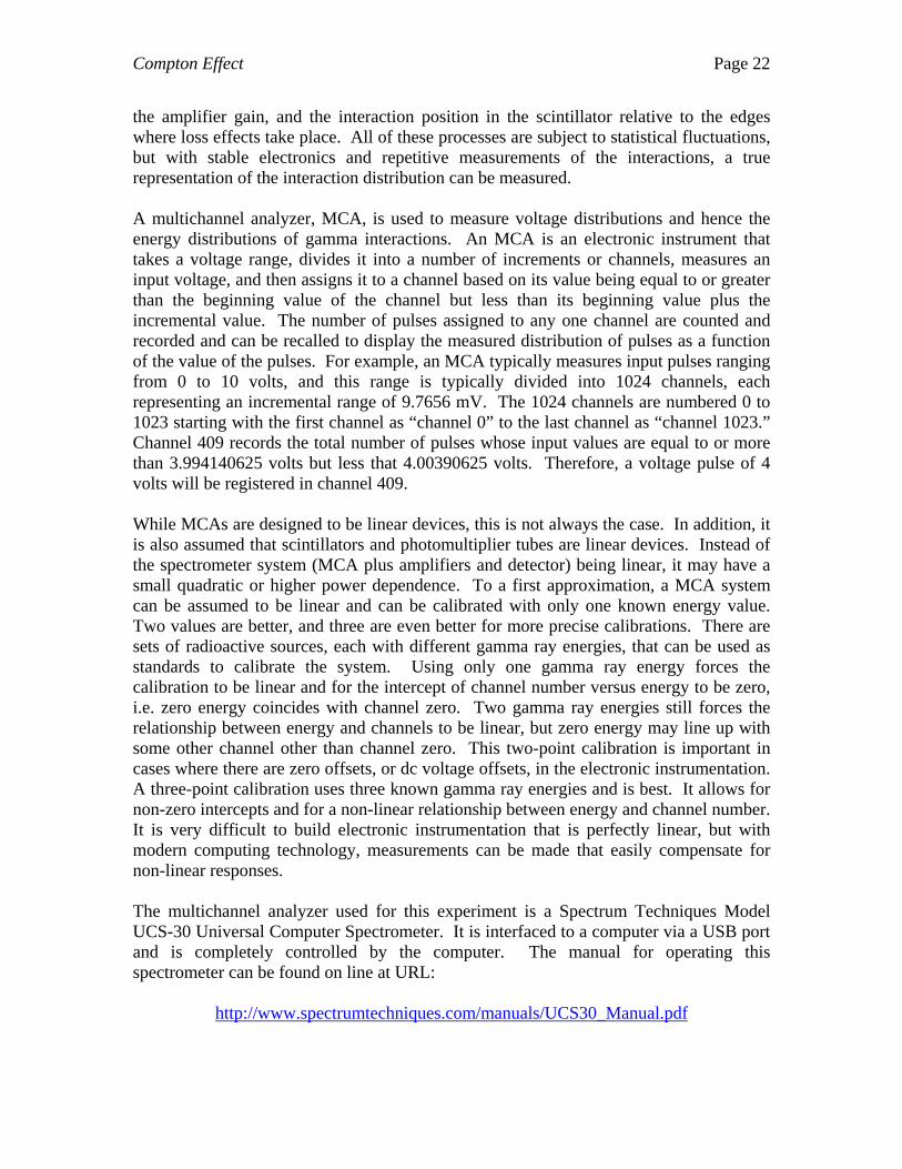
and should be referred to for a more thorough set of instructions. Only the salient information for a rudimentary operation and the essential components for performing the experiment will be covered here.

Figure 16. Schematic diagram of a multichannel analyzer illustrating the basic components. A simple schematic diagram of the UCS-30 multichannel analyzer is shown in Figure 16 and photos of the front and back panels of the instrument are shown in Figure 17. As shown in the schematic diagram, the detector requires a high voltage supply that is supplied by the USC-30. The signal generated by the detector is sent to the input of the pre-amplifier (“INPUT” BNC terminal on back of UCS-30 unit), and is then amplified by another amplifier within the UCS-30 instrument. Amplifer gain and high voltage settings are completely controlled with Spectrum Techniques UCS-30 software. The software for

operating the UCS-30 MCA unit may be started by clicking on the “UCX” icon, . This brings up the user interface as shown in Figure 18.

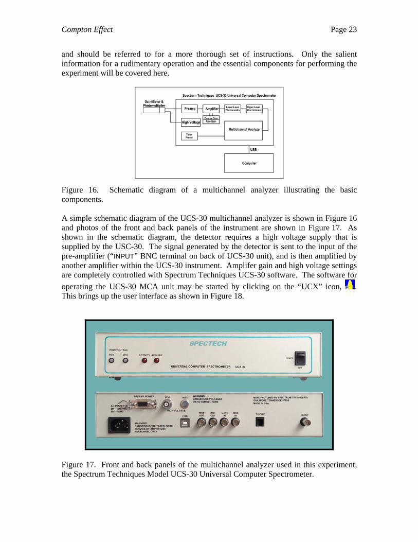
Figure 17. Front and back panels of the multichannel analyzer used in this experiment, the Spectrum Techniques Model UCS-30 Universal Computer Spectrometer.


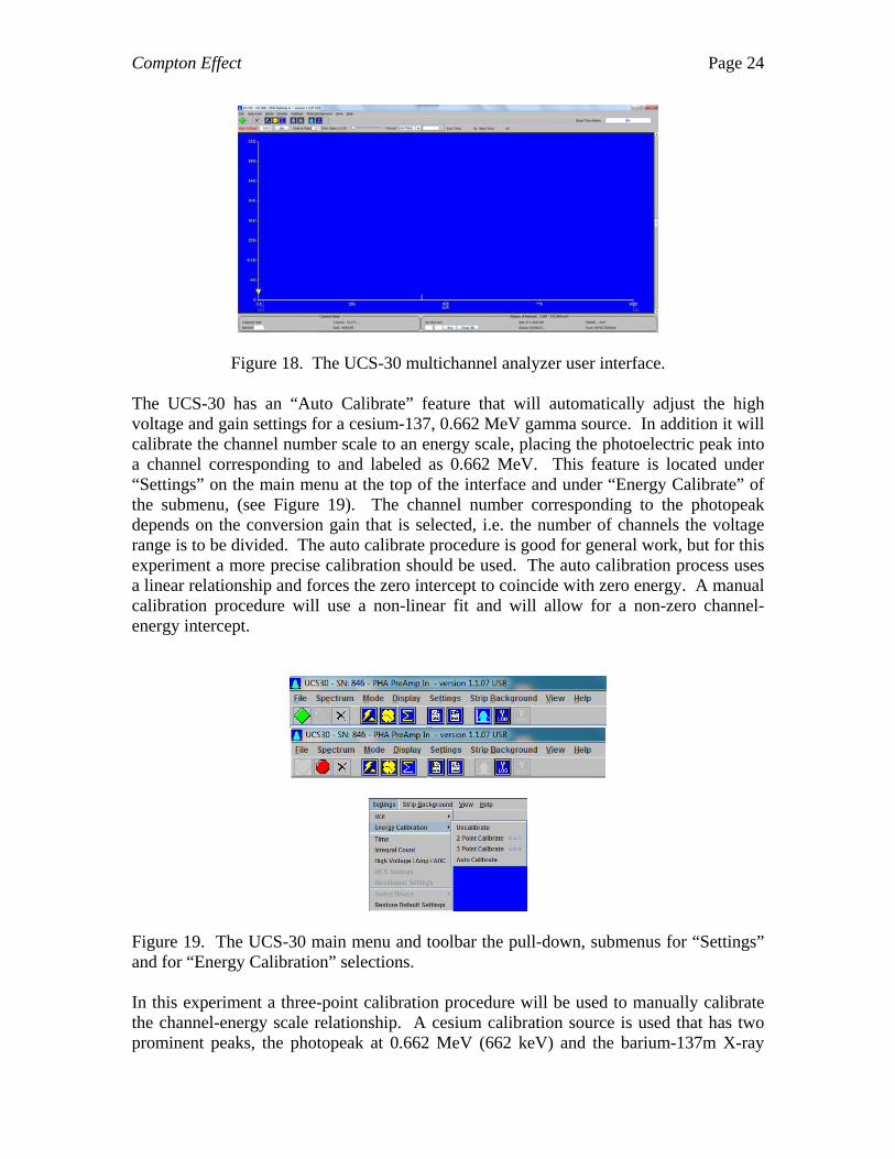
Figure 18. The UCS-30 multichannel analyzer user interface. The UCS-30 has an “Auto Calibrate” feature that will automatically adjust the high voltage and gain settings for a cesium-137, 0.662 MeV gamma source. In addition it will calibrate the channel number scale to an energy scale, placing the photoelectric peak into a channel corresponding to and labeled as 0.662 MeV. This feature is located under “Settings” on the main menu at the top of the interface and under “Energy Calibrate” of the submenu, (see Figure 19). The channel number corresponding to the photopeak depends on the conversion gain that is selected, i.e. the number of channels the voltage range is to be divided. The auto calibrate procedure is good for general work, but for this experiment a more precise calibration should be used. The auto calibration process uses a linear relationship and forces the zero intercept to coincide with zero energy. A manual calibration procedure will use a non-linear fit and will allow for a non-zero channel-energy intercept.

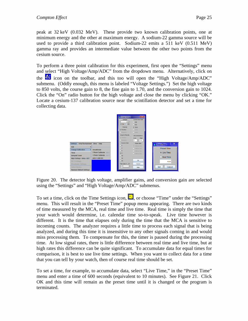
Figure 19. The UCS-30 main menu and toolbar the pull-down, submenus for “Settings” and for “Energy Calibration” selections. In this experiment a three-point calibration procedure will be used to manually calibrate the channel-energy scale relationship. A cesium calibration source is used that has two prominent peaks, the photopeak at 0.662 MeV (662 keV) and the barium-137m X-ray


peak at 32 keV (0.032 MeV). These provide two known calibration points, one at minimum energy and the other at maximum energy. A sodium-22 gamma source will be used to provide a third calibration point. Sodium-22 emits a 511 keV (0.511 MeV) gamma ray and provides an intermediate value between the other two points from the cesium source. To perform a three point calibration for this experiment, first open the “Settings” menu and select “High Voltage/Amp/ADC” from the dropdown menu. Alternatively, click on

the icon on the toolbar, and this too will open the “High Voltage/Amp/ADC” submenu. (Oddly enough, this menu is labeled “Voltage Settings.”) Set the high voltage to 850 volts, the course gain to 8, the fine gain to 1.70, and the conversion gain to 1024. Click the “On” radio button for the high voltage and close the menu by clicking “OK.” Locate a cesium-137 calibration source near the scintillation detector and set a time for collecting data.

Figure 20. The detector high voltage, amplifier gains, and conversion gain are selected using the “Settings” and “High Voltage/Amp/ADC” submenus.

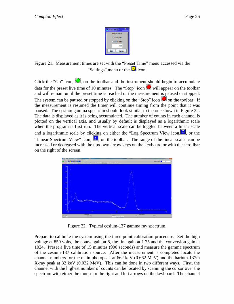
To set a time, click on the Time Settings icon, , or choose “Time” under the “Settings” menu. This will result in the “Preset Time” popup menu appearing. There are two kinds of time measured by the MCA, real time and live time. Real time is simply the time that your watch would determine, i.e. calendar time so-to-speak. Live time however is different. It is the time that elapses only during the time that the MCA is sensitive to incoming counts. The analyzer requires a little time to process each signal that is being analyzed, and during this time it is insensitive to any other signals coming in and would miss processing them. To compensate for this, the timer is paused during the processing time. At low signal rates, there is little difference between real time and live time, but at high rates this difference can be quite significant. To accumulate data for equal times for comparison, it is best to use live time settings. When you want to collect data for a time that you can tell by your watch, then of course real time should be set. To set a time, for example, to accumulate data, select “Live Time,” in the “Preset Time” menu and enter a time of 600 seconds (equivalent to 10 minutes). See Figure 21. Click OK and this time will remain as the preset time until it is changed or the program is terminated.


Figure 21. Measurement times are set with the “Preset Time” menu accessed via the

“Settings” menu or the icon.

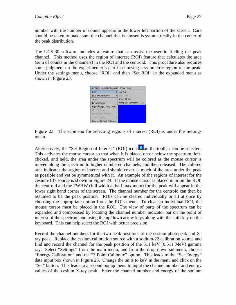
Click the “Go” icon, , on the toolbar and the instrument should begin to accumulate

data for the preset live time of 10 minutes. The “Stop” icon will appear on the toolbar and will remain until the preset time is reached or the measurement is paused or stopped.

The system can be paused or stopped by clicking on the “Stop” icon on the toolbar. If the measurement is resumed the timer will continue timing from the point that it was paused. The cesium gamma spectrum should look similar to the one shown in Figure 22. The data is displayed as it is being accumulated. The number of counts in each channel is plotted on the vertical axis, and usually by default is displayed as a logarithmic scale when the program is first run. The vertical scale can be toggled between a linear scale

and a logarithmic scale by clicking on either the “Log Spectrum View icon, , or the

“Linear Spectrum View” icon, , on the toolbar. The range of the linear scales can be increased or decreased with the up/down arrow keys on the keyboard or with the scrollbar on the right of the screen.

Figure 22. Typical cesium-137 gamma ray spectrum. Prepare to calibrate the system using the three-point calibration procedure. Set the high voltage at 850 volts, the course gain at 8, the fine gain at 1.75 and the conversion gain at 1024. Preset a live time of 15 minutes (900 seconds) and measure the gamma spectrum of the cesium-137 calibration source. After the measurement is completed locate the channel numbers for the main photopeak at 662 keV (0.662 MeV) and the barium-137m X-ray peak at 32 keV (0.032 MeV). This can be done in two different ways. First, the channel with the highest number of counts can be located by scanning the cursor over the spectrum with either the mouse or the right and left arrows on the keyboard. The channel


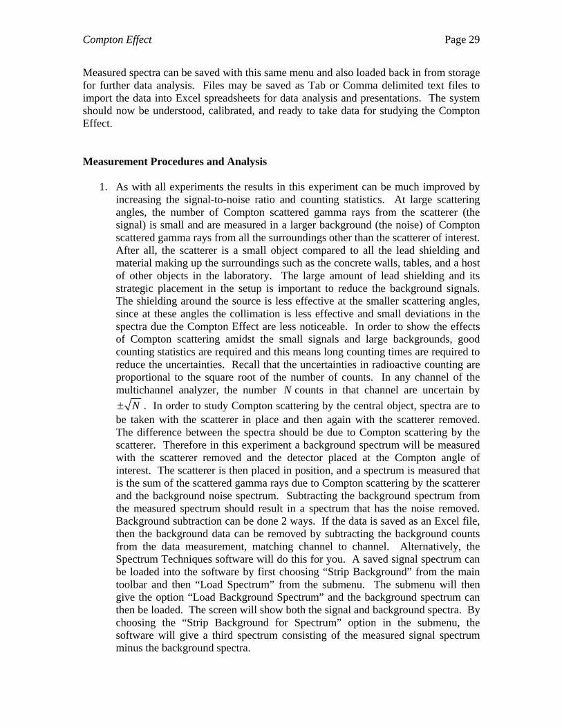
number with the number of counts appears in the lower left portion of the screen. Care should be taken to make sure the channel that is chosen is symmetrically in the center of the peak distribution. The UCS-30 software includes a feature that can assist the user in finding the peak channel. This method uses the region of interest (ROI) feature that calculates the area (sum of counts in the channels) in the ROI and the centroid. This procedure also requires some judgment on the experimenter’s part in choosing a symmetric region of the peak. Under the settings menu, choose “ROI” and then “Set ROI” in the expanded menu as shown in Figure 23.

Figure 23. The submenu for selecting regions of interest (ROI) is under the Settings menu.

Alternatively, the “Set Region of Interest” (ROI) icon on the toolbar can be selected. This activates the mouse cursor so that when it is placed on or below the spectrum, left-clicked, and held, the area under the spectrum will be colored as the mouse cursor is moved along the spectrum to higher numbered channels, and then released. The colored area indicates the region of interest and should cover as much of the area under the peak as possible and yet be symmetrical with it. An example of the regions of interest for the cesium-137 source is shown in Figure 24. If the mouse cursor is placed in or on the ROI, the centroid and the FWHW (full width at half maximum) for the peak will appear in the lower right hand corner of the screen. The channel number for the centroid can then be assumed to be the peak position. ROIs can be cleared individually or all at once by choosing the appropriate option from the ROIs menu. To clear an individual ROI, the mouse cursor must be placed in the ROI. The view of parts of the spectrum can be expanded and compressed by locating the channel number indicator bar on the point of interest of the spectrum and using the up/down arrow keys along with the shift key on the keyboard. This can help select the ROI with better precision. Record the channel numbers for the two peak positions of the cesium photopeak and X-ray peak. Replace the cesium calibration source with a sodium-22 calibration source and find and record the channel for the peak position of the 511 keV (0.511 MeV) gamma ray. Select “Settings” from the main menu, and from the drop down submenu, choose “Energy Calibration” and the “3 Point Calibrate” option. This leads to the “Set Energy” data input box shown in Figure 25. Change the units to keV in the menu and click on the “Set” button. This leads to a second popup menu to input the channel number and energy values of the cesium X-ray peak. Enter the channel number and energy of the sodium


photopeak for calibration point 2 and then repeat for the cesium photo peak for point 3. This will calibrate the channel scale, and it will now be calibrated in keV units. Cursor values on the interface will also now appear in keV units.

Figure 24. Screen showing regions of interest (ROI).

Figure 25. Energy calibration data input boxes.

The UCS-30 MCA should now be calibrated. The values for this setup and calibration should be saved by choosing “File” from the main menu and “Save Setup” from the pulldown menu. This setup can be recalled and loaded using the same menus for any other future measurements.

Figure 26. File menu for saving data.


Measured spectra can be saved with this same menu and also loaded back in from storage for further data analysis. Files may be saved as Tab or Comma delimited text files to import the data into Excel spreadsheets for data analysis and presentations. The system should now be understood, calibrated, and ready to take data for studying the Compton Effect. Measurement Procedures and Analysis

1. As with all experiments the results in this experiment can be much improved by increasing the signal-to-noise ratio and counting statistics. At large scattering angles, the number of Compton scattered gamma rays from the scatterer (the signal) is small and are measured in a larger background (the noise) of Compton scattered gamma rays from all the surroundings other than the scatterer of interest. After all, the scatterer is a small object compared to all the lead shielding and material making up the surroundings such as the concrete walls, tables, and a host of other objects in the laboratory. The large amount of lead shielding and its strategic placement in the setup is important to reduce the background signals. The shielding around the source is less effective at the smaller scattering angles, since at these angles the collimation is less effective and small deviations in the spectra due the Compton Effect are less noticeable. In order to show the effects of Compton scattering amidst the small signals and large backgrounds, good counting statistics are required and this means long counting times are required to reduce the uncertainties. Recall that the uncertainties in radioactive counting are proportional to the square root of the number of counts. In any channel of the multichannel analyzer, the number N counts in that channel are uncertain by

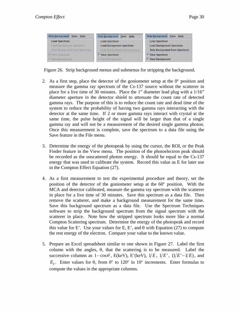
N . In order to study Compton scattering by the central object, spectra are to be taken with the scatterer in place and then again with the scatterer removed. The difference between the spectra should be due to Compton scattering by the scatterer. Therefore in this experiment a background spectrum will be measured with the scatterer removed and the detector placed at the Compton angle of interest. The scatterer is then placed in position, and a spectrum is measured that is the sum of the scattered gamma rays due to Compton scattering by the scatterer and the background noise spectrum. Subtracting the background spectrum from the measured spectrum should result in a spectrum that has the noise removed. Background subtraction can be done 2 ways. If the data is saved as an Excel file, then the background data can be removed by subtracting the background counts from the data measurement, matching channel to channel. Alternatively, the Spectrum Techniques software will do this for you. A saved signal spectrum can be loaded into the software by first choosing “Strip Background” from the main toolbar and then “Load Spectrum” from the submenu. The submenu will then give the option “Load Background Spectrum” and the background spectrum can then be loaded. The screen will show both the signal and background spectra. By choosing the “Strip Background for Spectrum” option in the submenu, the software will give a third spectrum consisting of the measured signal spectrum minus the background spectra.


Figure 26. Strip background menus and submenus for stripping the background.

2. As a first step, place the detector of the goniometer setup at the 0 position and measure the gamma ray spectrum of the Cs-137 source without the scatterer in place for a live time of 30 minutes. Place the 1” diameter lead plug with a 1/16” diameter aperture in the detector shield to attenuate the count rate of detected gamma rays. The purpose of this is to reduce the count rate and dead time of the system to reduce the probability of having two gamma rays interacting with the detector at the same time. If 2 or more gamma rays interact with crystal at the same time, the pulse height of the signal will be larger than that of a single gamma ray and will not be a measurement of the desired single gamma photon. Once this measurement is complete, save the spectrum to a data file using the Save feature in the File menu.

3. Determine the energy of the photopeak by using the cursor, the ROI, or the Peak

Finder feature in the View menu. The position of the photoelectron peak should be recorded as the unscattered photon energy. It should be equal to the Cs-137 energy that was used to calibrate the system. Record this value as E for later use in the Compton Effect Equation (27).

4. As a first measurement to test the experimental procedure and theory, set the

position of the detector of the goniometer setup at the 60 position. With the MCA and detector calibrated, measure the gamma ray spectrum with the scatterer in place for a live time of 30 minutes. Save this spectrum as a data file. Then remove the scatterer, and make a background measurement for the same time. Save this background spectrum as a data file. Use the Spectrum Techniques software to strip the background spectrum from the signal spectrum with the scatterer in place. Note how the stripped spectrum looks more like a normal Compton Scattering spectrum. Determine the energy of the photopeak and record this value for E’. Use your values for E, E’, and with Equation (27) to compute the rest energy of the electron. Compare your value to the known value.

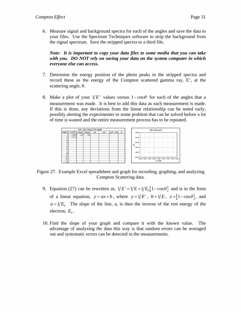
5. Prepare an Excel spreadsheet similar to one shown in Figure 27. Label the first

column with the angles, , that the scattering is to be measured. Label the successive columns as 1 cos , E(keV), E’(keV), 1 E , 1 'E , (1 ' 1 )E E , and

0E . Enter values for , from 0 to 120 in 10 increments. Enter formulas to

compute the values in the appropriate columns.


6. Measure signal and background spectra for each of the angles and save the data to your files. Use the Spectrum Techniques software to strip the background from the signal spectrum. Save the stripped spectra to a third file.

Note: It is important to copy your data files to some media that you can take with you. DO NOT rely on saving your data on the system computer in which everyone else can access.

7. Determine the energy position of the photo peaks in the stripped spectra and

record these as the energy of the Compton scattered gamma ray, E’, at the scattering angle, .

8. Make a plot of your 1 'E values versus 1 cos for each of the angles that a

measurement was made. It is best to add this data as each measurement is made. If this is done, any deviations from the linear relationship can be noted early, possibly alerting the experimenter to some problem that can be solved before a lot of time is wasted and the entire measurement process has to be repeated.

Figure 27. Example Excel spreadsheet and graph for recording, graphing, and analyzing Compton Scattering data.

9. Equation (27) can be rewritten as, 01 ' 1 1 1 cosE E E and is in the form

of a linear equation, y ax b , where 1 'y E , 1b E , 1 cosx , and

01a E The slope of the line, a, is then the inverse of the rest energy of the

electron, 0E .

10. Find the slope of your graph and compare it with the known value. The

advantage of analyzing the data this way is that random errors can be averaged out and systematic errors can be detected in the measurements.


Questions: 1. What is the maximum energy a backscattered gamma ray can have when it is backscattered from a material into a detector, regardless of the initial energy of the incident gamma ray photon? 2. What is the maximum energy given to an electron by a Compton scattered gamma ray whose initial energy is 0.662 MeV? 3. List sources of background radiation in the measurements of a gamma ray spectrum in the Compton scattering experiment.


Compton Effect Learning Objectives

1. To learn the significant parts of a gamma ray spectrum: the photopeak, the Compton

Knee, X‐ray Production, and positron annihilation and how they are generated

2. To learn the basic principles for the theory of the Compton Effect (Laws of Conservation

of Energy and Momentum, Relativistic Mechanics).

3. To learn how a gamma ray interacts with a scintillator and what causes the generation

of light; how a voltage pulse is produced in a photomultiplier tube.

4. To learn sources of background radiation and how to minimize their effect on the

measurements.

5. To learn the equation for the Compton Effect and how to use your data and

measurements to verify the equation.

6. To learn calibration techniques for a multichannel analyzer and gamma ray spectroscopy

system.

Compton Effect Required Reporting Components

1. Measured innate, uncorrected multichannel analyzer spectrum generated by a scatterer

via the Compton Effect for each angle (include each spectrum).

2. Background multichannel analyzer spectrum generated with the scatterer removed for

each angle (include each spectrum).

3. Corrected multichannel analyzer spectrum generated by subtracting the background

spectrum with the scatterer removed from the setup at each of scattering angles

(include each spectrum).

4. A plot of 1

'E values versus 1 cos .

5. The measured value of 0E from slope of plot.


Compton Effect Experimental Procedure

(Condensed version by Jacob Wessels, May 27, 2014)

Procedure

1. First, turn on the computer. Make sure the UCS 30 multichannel analyzer (MCA)

is turned on and that it is hooked up to the computer and the photomultiplier tube.

2. Open the USX program on the computer desktop.

3. There are two kinds of time measured by the MCA, real time and live time. Real

time is time that your watch would determine. Live time is the time that elapses

only during the time that the MCA is sensitive to incoming counts. The analyzer

requires a little time to process each signal that is being analyzed, and during this

time it is insensitive to any other signals coming in. To compensate for this, the

timer is paused during the processing time. At low signal rates, there is little

difference between real time and live time, but at high rates this difference can be

quite significant. To accumulate data for equal times for comparison, it is best to

use live time settings.

4. Calibrate the MCA using a 3 point calibration. To do this, first use the Auto

Calibrate option. Place the small cesium-137 source in the slot in the lead block.

Then, select Auto Calibrate under Settings and then Energy Calibration. It will

adjust the high voltage and gain settings for a cesium-137 source.

5. Then, record a cesium-137 spectrum for 600 seconds of live time. This will be

under Settings and then Time. Write down the channel positions at which the

leftmost, smallest peak and the larger peak at the right are. The left one should be

at about channel 32, and the right should be at about 662.

6. Remove the cesium-137 source and place the sodium-22 source in the slot.

Record another spectrum for 600 seconds. Then, record the position of the large

peak in this spectrum. This should be near channel 511.

7. Click 3-Point, which is under Settings and then Energy Calibration. A series of

windows will appear. Enter keV in the first. For the next three windows, enter the

channels of the three peaks in numerical order, along with the energy values


which they should represent, which are 32 keV, 511 keV, and 662 keV,

respectively. The MCA should now be calibrated.

8. Once the program has been calibrated, be sure to use these settings for all future

measurements. The setup can be saved by selecting Save Setup under the File

menu. This setup can then be recalled and loaded when needed for future

measurements using the Load Setup option.

9. Start recording data at zero degrees. The scatterer does not need to be in place for

this position. It is also not necessary to worry about background noise for this

angle. Start by pressing the green Start Counts button. The red Stop Counts button

will appear and will remain until the preset time is reached. The system can be

paused or stopped by clicking the Stop Counts button. If the measurement is

resumed, the timer will continue timing from the point at which it was paused.

10. When the photomultiplier tube has direct line-of-sight with the large cesium

source, then the plug with the 1/8 inch hole should be inserted into the lead block

to decrease the number of counts. If this is not done, the large cesium-137 source

is so strong that multiple gamma rays hit the sensor at the same time, so the

sensor thinks that they comprise one higher-energy gamma ray. This skews the

peak upwards in energy.

11. The different channels and the energy value for each channel are displayed on the

x axis, and the number of counts in each channel is plotted on the y axis.

12. Save the completed spectrum as a Spectrum File and as a Tab Separated File,

which can be opened in Excel.

13. Move the swinging arm to 10° and collect data with a live time limit of ____

seconds. Do this initially with the scatterer present and then with the scatterer

removed. Save each spectrum.

14. At large scattering angles, the number of Compton scattered gamma rays from the

scatterer (the signal) is small and are measured in a larger background (the noise)

of Compton scattered gamma rays from all the other surroundings. The scatterer

is a small object compared to all the material making up the surroundings. The

small amount of signal requires long counting times for larger angles.


15. The spectrum without the scatterer present measures background noise not due to

the Compton Effect on the scatterer.

16. With the spectrum with the scatterer pulled up, use the option Load Background

Spectrum to load the spectrum without the scatterer. Then, use Strip Background

from Spectrum to remove the noise. These options are found under the Strip

Background menu. This should make the peak due to Compton scattering more

obvious. Record the energy value of the Compton peak.

17. Data should be recorded for angles of 0, 10, 20, 30, 40, 50, 60, 70, 80,

90, 100, 110, and 120 degrees.

18. The set time limit will need to be increased as the angle increases. Past about 90

degrees, this may need to be increased to as much as two hours.

Analysis

1. Open an Excel spreadsheet.

2. Place the angles at which results were measured in the first column of the

spreadsheet. Place the energies of the Compton scattered gamma rays at each

angle in the third column.

3. Use a formula to create a second column of the values of [1-cosθ] for each angle.

4. Use a formula to create a fourth column of 1 1

'E E

for the energy value found

for each angle.

5. Insert a scatter plot with only markers (in the Charts menu under Insert), with [1-

cosθ] on the x axis and the energy of the scattered photon minus the energy of the

incident photon 1 1

'E E

on the y axis.

6. Right click on a data point. Select the option Format Trendline. Select Linear and

Display Equation on Chart. Then, click Close.

7. Since the equation of Compton scattering is of the form 0

1 1 11 cos

'E E E

then the slope of the trendline should be equal to 0

1

E, which is 1 over the rest

energy of the electron. (The rest energy of an electron is 511 keV.)


8. Compute the percent difference between your experimental value for the slope

and the calculated value of 0

1

E. Record this value in your Excel spreadsheet.

Documents

The Compton Effect-- Compton Scattering and … Compton Effect-- Compton Scattering and Gamma Ray Spectroscopy by Dr. James E. Parks Department of Physics and Astronomy 401 Nielsen