The Compromise Game:

Two-sided Adverse Selection in the Laboratory ∗

Juan D. CarrilloUniversity of Southern California

and CEPR

Thomas R. PalfreyCalifornia Institute of Technology

April 9, 2008

∗Part of this research was conducted while the first author was visiting Caltech.The hospitality of the hosting institution is greatly appreciated. We also gratefully ac-knowledge the financial support of the National Science Foundation (SES-0079301, SES-0450712, SES-0094800), The Princeton Laboratory for Experimental Social Science, andThe Princeton Center for Economic Policy Studies. We thank seminar audiences atCollege de France, Princeton University, Universidad Carlos III, Universitat Autonoma deBarcelona, University of Pennsylvania, the Fundacion Ramon Areces Conference on Ex-perimental and Behavioral Economics in December 2006, and 2006 ESA meeting in Tucsonfor comments, and Shivani Nayyar, Stephanie Wang, and Rumen Zarev for research assis-tance. Corresponding addresses: Juan D. Carrillo, Department of Economics, Universityof Southern California, Los Angeles, CA 90089-0253, <juandc@usc.edu>. Thomas R. Pal-frey, Division of the Humanities and Social Sciences, California Institute of Technology,Pasadena, CA 91125, <trp@hss.caltech.edu>.

Abstract

We analyze a game of two-sided private information characterized by ex-treme adverse selection, and study a special case in the laboratory. Eachplayer has a privately known ”strength” and can decide to fight or com-promise. If either chooses to fight, there is a conflict; the stronger playerreceives a high payoff and the weaker player receives a low payoff. If bothchoose to compromise, conflict is avoided and each receives an intermediatepayoff. The only equilibrium in both the sequential and simultaneous ver-sions of the game is for players to always fight, independent of their ownstrength. In our experiment, we have two main treatments: whether thegame is played simultaneously or sequentially; and the magnitude of the in-termediate payoff. We observe: (i) frequent compromise; (ii) significantlymore fighting the lower the compromise payoff; (iii) significantly less fightingby first than second movers; and (iv) almost no evidence of learning. Weexplore several theories of cognitive limitations in an attempt to understandthe reasons underlying these anomalous findings, including quantal responseequilibrium, cognitive hierarchy, and cursed equilibrium.

JEL classification: C92, D82.

Keywords: two-sided private information, adverse selection, laboratory ex-periment, behavioral game theory, quantal response equilibrium, cognitivehierarchy, cursed equilibrium.

1 Introduction

A major insight from theoretical research in information economics is thatprofitable agreements may be severely impeded by private information, andcan even dry up completely. This was nicely illustrated in Akerlof’s (1970)famous market for lemons example and studied in further detail by My-erson and Satterthwaite (1983) in a context of optimal contracting withtwo-sided private information. More generally, no-trade theorems (Milgromand Stokey (1982), Morris (1994)) show that rational, expected utility max-imizing, Bayesian economic agents will not trade with each other on thebasis of private information alone.

In this paper, we study the other side of the coin, namely a situationwhere exchanges (or other type of agreements) are not mutually beneficialand ask the following question: can private information induce agents toreach agreements that one of them will (ex post) regret? An all-too-familiarexample, war, illustrates the problem. Suppose there are two nations, eitherof which would be better off if conquering the other nation, compared topeaceful coexistence, and would be worse off being conquered. If there isa war, whichever country is strongest conquers the other one. Each nationchooses to either ”attack” or ”not attack”. They remain in peaceful coex-istence if both choose not to attack, and a war ensues otherwise. If oneformalizes this problem, it is obvious that the strongest nation has alwaysan incentive to attack the weakest one. Thus, a war is inevitable. Moreinterestingly, the equilibrium is also war if the leader of each nation knowsits own military strength but knows only the probability distribution of theother nation’s strength (and therefore is uncertain over his chances of win-ning). This would be true, for example, even if the benefits of winning thewar were only slightly greater than the peace benefits, the costs of losing thewar were enormous, and the uncertainty about the other nation’s strengthwere large. The logic is much like the unraveling argument in adverse selec-tion games. In deciding whether to attack or not, optimal decision makingrequires the agents to condition on their opponent choosing ”not attack”.Because weaker opponents are the ones who do not attack, this conditioningwill lead stronger opponents to attack. Therefore, there will be a marginalstrength level which is indifferent between peace and forcing a war. Butthis calculus will lead the opponent’s marginal non-attackers to attack, andso forth. The only equilibrium is for the marginal strength type to be theweakest type. As developed in section 2.1, the same logic applies to othersituations where parties with conflicting goals and private information can

1

reach an agreement that cannot ex post benefit both parties: litigation,electoral debates, and firm competition.

We report here an experiment that analyzes behavior in several varia-tions of this two-sided asymmetric information environment in the labora-tory. In all the variations, the equilibrium outcome predicted by the theoryis the same: fighting ensues with probability one. We obtain three mainresults, which are inconsistent with standard game theory. First and fore-most, fighting occurs much less often than predicted by theory. Ratherthan 100%, we observe fight rates in the range of 50%-70%. The outcomecharacterized by both agents compromising arises with surprising frequency,nearly one-quarter of the time in some sessions. In terms of our exampleit means that, contrary to the predictions of game theory, a war can beavoided if the military strengths of countries are privately (rather than pub-licly) known. Second, fight rates are affected by the compromise payoff. Inboth the sequential and simultaneous treatments, agents are less likely tofight the higher the compromise payoff. Third, in the sequential version,the strategies of first and second movers are different in two ways: secondmovers are more likely to fight than first movers, and the behavior of sec-ond movers is more responsive to strength and less erratic than that of firstmovers.

We also obtain some findings about individual behavior. Individualchoice is consistent with the use of cutpoint strategies: fight if and onlyif strength is above a certain critical threshold. However, instead of the cut-points being at (or at least close to) the minimum strength, as predicted bythe theory, we find that players use cutpoints in an intermediate range. Theuse of cutpoint strategies indicates that subjects have some understanding ofthe game, and the source of violations of equilibrium has to do with the cog-nitive difficulty to choose the cutpoint optimally. Perhaps more interesting,we find substantial heterogeneity in the choice of cutpoints across subjects,and also important differences in the distribution of cutpoints across treat-ments. Finally, all the results are robust with respect to experience, that is,there is little evidence of learning.

We then explore three recent theories of cognitive limitations in games,and analyze the data to investigate the extent to which the insights fromthese alternative theories can account for these anomalies. The three ap-proaches we explore are equilibrium stochastic choice, levels of strategic so-phistication, and naıve belief formation. The specification of our modelsfor these three approaches are, respectively, the logit specification of Quan-tal Response Equilibrium theory (QRE); the Poisson specification of the

2

Cognitive Hierarchy model (CH); and a stochastic choice version of CursedEquilibrium (CE). The estimated parameters for each model are relativelyconstant across treatments. However, there are some important differencesin the predictions, that lead to differences in the fit of the models. An im-portant result is that only the QRE model captures the tendency of secondmovers to fight more often than first movers. The CH and CE models cap-ture the aggregate tendency of players to fight with probability close to onewhen their strength is sufficiently high and with probability close to zerowhen their strength is sufficiently low. The CH model predicts that the dis-tribution of individual cutpoints will be multimodal, clustered around threeor four numbers, which is not reflected in the data. Finally, the best fitis obtained with a hybrid of QRE and CE, which combines cursedness andstochastic choice.

2 The theoretical model

We analyze the incentives of agents to compromise when they have conflict-ing objectives and asymmetric information. To this end, we study a class ofgames that have unique Nash equilibrium outcomes in which a compromiseis never reached.

2.1 Some introductory examples

Consider two agents who must decide whether to split a surplus in a pre-specified manner (compromise) or try to reap all the benefits (no-compromise).Both agents have private but imperfect information about their likelihoodof obtaining the benefits if they do not compromise and, possibly, its valuealso. The ex post sum of utilities may be higher or lower under compromisethan under no-compromise.

A myriad of situations fit this general description, in addition to the ex-ample of international conflict described in the introduction. In a litigation,the defendant may offer a settlement to the plaintiff which can be acceptedor not. Both parties have private knowledge of the strength of their caseand the bias of the jury. In an electoral campaign, each candidate can driveits rival into a public debate, where some qualities of the contenders arerevealed to voters, which affects the electoral outcome. In the absence of adebate, voters must rely on expected qualities. In a product market compe-tition, firms offering horizontally differentiated products may start an R&Drace. The winner monopolizes the market and the probability of winning

3

is proportional to the privately known quality of their research department.Alternatively, firms can avoid the race and share the market. In all thesecases, there are only two possible outcomes: settlement, peace, no debate,market sharing vs. trial, war, debate, R&D race. The first outcome needsthe agreement of both players whereas each player can unilaterally force thesecond outcome. Payoffs depend on the state of the world, which is notrealized or revealed until after all players have acted. Also, the utility ofagents under the different outcomes may depend on some exogenously givenprivate information parameters. Payoffs under agreement are typically de-termined by the status quo situation, whereas payoffs under no-agreementare typically determined by a winner-takes-all rule. More generally, in theno-agreement outcome, there is always one (ex post) winner and one (expost) loser relative to the agreement outcome. The total surplus from com-promise varies across these different applications, although we show belowthat the equilibrium does not depend on the compromise payoffs. Warsare typically costly and socially inefficient, so there is as peace dividend.Litigation also involves a waste of resources when compared to early set-tlements (but not compared to last minute settlements). Electoral debatesare roughly neutral if candidates are only interested in winning the election.However, they provide information regarding the merits of different propos-als, which can be valuable if candidates care also about policy outcomes. Asfor market competition, the profits of a monopolist are typically higher thanthe sum of profits of two duopolists, which suggests that firms’ surplus isincreased when they fight for supremacy rather than splitting the market.1

2.2 Formalizing the game

We formalize the problem as follows. Denote by si ∈ Si and sj ∈ Sj the pri-vately known ”strength” of agents i and j, with i, j ∈ {1, 2} and i 6= j (casestrength, military capacity, politician’s talent, research quality). These val-ues are drawn from continuous and commonly known distributions Fi(si | sj)possibly different and possibly correlated. For technical convenience, we as-sume strictly positive densities fi(si | sj) for all si and sj . Agent i choosesaction ai ∈ A = {ρ, φ}, where ρ stands for ”retreat” and φ for ”fight”. Ifa1 = a2 = ρ, there is compromise (settlement, peace, no debate, no race)and the payoff of agent i is βi(s1, s2). Otherwise, there is no-compromise(trial, war, debate, race) and the payoff of agent i is αi(s1, s2) if si > sj

and γi(s1, s2) if si < sj , with αi(s1, s2) > βi(s1, s2) > γi(s1, s2) for all

1In these examples, we are not including the welfare of third parties such as society,voters or consumers. These are also likely to be different across outcomes.

4

i, s1, s2. Note that, ex post, a compromise is always beneficial for one agentand detrimental for the other. The pair of strengths (si, sj) determines thewinner and the loser. Payoffs under compromise and no-compromise areexogenously given, although they may be unknown at the time of makingthe decision if they depend on (s1, s2). Last, depending on the context, thesocially efficient action may be compromise or no-compromise or it may evenbe a zero-sum game: αi(s1, s2) + γj(s1, s2) R βi(s1, s2) + βj(s1, s2) for allsi > sj .

2.3 Equilibrium

Given this structure, we can analyze the Perfect Bayesian Equilibrium (PBE)for the sequential version of the game where agent 1 moves first and agent2 moves second. We have the following result.

Proposition 1 In all PBE of the game, the outcome is ”no-compromise”.

Proof. Suppose that there exist two sets S1 j S1 and S2(S1) j S2 such thatin a PBE of the game a1(s1) = ρ and a2(s2) = ρ with positive probabilityfor all s1 ∈ S1 and s2 ∈ S2(S1).2 Denote by s1 = max

s1∈S1

and s2 = maxs2∈S2(S1)

.

According to this PBE, once agent 2 has observed a1 = ρ, the followinginequality must be satisfied:∫

s1∈S1

β2(s1, s2)dF1(s1 | s1 ∈ S1, s2) >∫

s1∈S1∩s1<s2

α2(s1, s2)dF1(s1 | s1 ∈ S1, s2)

+∫

s1∈S1∩s1>s2

γ2(s1, s2)dF1(s1 | s1 ∈ S1, s2) ∀ s2 ∈ S2(S1)

where the l.h.s. is agent 2’s expected payoff if a2 = ρ and the r.h.s. is hisexpected payoff if a2 = φ. This condition must hold in particular for s2 = s2.Since α2(s1, s2) > β2(s1, s2) > γ2(s1, s2), the inequality necessarily impliesthat s1 < s2 must be binding at least for some s1 ∈ S1. Therefore, s2 < s1.Now, agent 1’s decision is relevant only if a2 = ρ. Thus, for the strategydescribed above to be a PBE, the following inequality must also hold:∫

s2∈S2(S1)β1(s1, s2)dF2(s2 | s1) >

∫s2∈S2(S1)∩s2<s1

α1(s1, s2)dF2(s2 | s1)

+∫

s2∈S2(S1)∩s2>s1

γ1(s1, s2)dF2(s2 | s1) ∀ s1 ∈ S1

2Positive probability rather than probability 1 takes care of pure and mixed strategiesat the same time.

5

Using the same reasoning as before, s1 < s2. Since both inequalities cannotbe satisfied at the same time, S1 6= ∅ and S2(S1) 6= ∅ cannot both occur inequilibrium. �

The intuition is simple. In this class of games, agents know that goodnews for them is bad news for their rival. Thus, they have opposite interestson when to reach a compromise. As a result, whenever one agent wants tocompromise, the other should not want to. For instance, country 1 has anincentive to stay in peaceful coexistence whenever its military strength s1

is low. However, this is precisely when country 2 wants to force a war. Inother words, in these games, one agent’s gain is always the other agent’s loss(of same or different magnitude, it does not matter). Since a compromiseis broken as soon as one agent does not find it profitable, the fact thatan agent wants to deal implies that the other should not accept it, andvice versa. The bottom line is that, in equilibrium, compromises are neverpossible. We want to stress the generality of this result, which holds forany distribution of strengths (the same or different for both players) andany correlation between the players’ strengths. Since the results holds forany payoffs satisfying αi > βi > γi, it means that introducing risk-aversionwould not change the outcome of the game either. Last, the result is alsounchanged if agents play simultaneously. Indeed, the only difference withthe sequential game is that agent 2 will not compare his options conditionalon having observed the choice of agent 1. However, this does not make anydifference since, both in the sequential and the simultaneous versions, eachagent knows that his action is only relevant if the rival offers a compromise.Thus the outcome of the Bayesian Nash Equilibrium (BNE) is, just like forthe PBE, always no-compromise. This result is summarized as follows.

Corollary 1 The outcome of the game is still ”no-compromise” if agentsare risk-averse and if they announce their strategy simultaneously.

3 Laboratory experiment

3.1 Description of the game

This is a simplified version of the game described earlier. Each agent inde-pendently draws a number from a uniform distribution on [0, 1] and privatelyobserves their own number, which we refer to as the player’s strength, si.Agent 1 chooses whether to ”fight”, φ, or ”retreat”, ρ. If 1 chooses φ, thenthe game ends. The agent with highest strength receives a win payoff Hand the other agent receives a lose payoff L (< H). If agent 1 chooses ρ,

6

then it is agent 2’s turn. If agent 2 chooses φ, then as before, the agent withhighest strength receives a payoff of H and the other receives a payoff of L.If, instead, agent 2 also chooses ρ, then agent 1 and agent 2 each obtains apre-specified ”compromise payoff” M , where L < M < H. Thus, the mainsimplification relative to the theoretical model presented in section 2 is thatthe win, lose and compromise payoffs are all independent of (s1, s2). Eachplayer’s strength only affects payoffs via the likelihood of winning underno-compromise. We look at several variations on this game.3

Variant 1. H = 1, L = 0, M = .50 with sequential move.Variant 2. H = 1, L = 0, M = .39 with sequential move.Variant 3. H = 1, L = 0, M = .50 with simultaneous move.Variant 4. H = 1, L = 0, M = .39 with simultaneous move.

In our design, the total surplus under compromise is either smaller than(M = .39) or equal to (M = .50) the total surplus under no compromise. Asdiscussed earlier, this specific choice of parameters fits some examples (firmcompetition, electoral debate) better than others (military conflict, litiga-tion). There were at least two reasons for focusing on these values. First,the M = .50 is a natural benchmark, corresponding to a constant sum game,where there is no difference in the efficiency of the fight and compromise out-comes. Second, we wanted to choose another value of M because the variousbehavioral theories we were testing all predict a negative comparative staticeffect of M on the probability of fighting. Changes in either direction wouldallow us to test this. Our choice of a lower value of M was made because wethought it was the more interesting direction, since for M < .5 always fight-ing is not only still the unique Nash equilibrium but is also ex ante efficientand ex ante fair. This allows us to better distinguish social preference orfairness-based explanations for excessive compromise (see section 5.5) frombehavioral models based on cognitive limitations (see sections 5.1 to 5.4),and also gives Nash equilibrium its best shot. If the excessive compromisedisappears, this would lend support for social preference theories based onex ante fairness and efficiency, whereas, if the excessive compromise persists,it lends support for the models of cognitive limitations.

3.2 Relation to the experimental literature

Some related games have been studied in the laboratory. Below we describe(from most to least similar) two simultaneous games of multi-sided asymmet-

3The nominal payoffs in the experiment are: H = 95, L = 5, M ∈ {50, 40}. We presenthere the scaled version (x− 5)/90.

7

ric information, two sequential games of one-sided asymmetric informationand one static game of full information.

The betting game (Sonsino et al. (2001), Sovic (2004), Camerer et al.(2006)). An asset yielding a fixed surplus can be traded between agentswho have private information. Trade occurs only if both agents agree. Asin our game, all the BNE imply no trade. There are three main differences.First, the risky outcome requires agreement in the betting game whereasthe safe outcome requires agreement in the compromise game. Second, theinformation structure is simpler than in ours: there are only four possiblestates, and in two of them one agent has full information. The commonknowledge of this information partition triggers very naturally unravelingto no-trade. This special partition is also likely to facilitate learning. Third,a sequential version of the betting game has not been studied.

Auction of a common value good and the winner’s curse (Kagel andLevin, 2002). As in our game, agents will play suboptimally if they donot anticipate the information contained in the rival’s action. Our gameallows for some simple comparative statics (different timings and differentcompromise payoffs). Also, our BNE and PBE are simple to compute.

Adverse selection game (Akerlof, 1970). This game also predicts someunraveling. However, the robust conclusion is the existence of a cutoff belowwhich there is agreement or trade and above which there is not. This cutoffcan be the lower bound (i.e., never agree as in our game), but it can alsobe the upper bound (i.e., always agree) or an interior value, depending onthe parameters of the game. Samuelson and Bazerman (1985) show thatthe probability that buyers engage in unfavorable trades is increasing in thecomplexity of the adverse selection game. Holt and Sherman (1994) provethat buyers may underbid or overbid depending on the treatment conditions.Note that because it is one-sided asymmetric information, the buyer’s actionhas no signaling value. There have also been several market experimentswith informed sellers and asymmetric information about product quality(Lynch et al., 1984).

Blind bidding game (Forsythe et al., 1989). This experiment determineswhether an informed seller reveals the quality of his good to an uninformedbuyer. Full revelation occurs because the seller with the highest qualitygood has always an incentive to announce it, then so does the seller withsecond highest quality good, and so on. However, there is no role for thekey effect of our game, namely the anticipation of information conveyed bythe rival’s action.

Beauty contest (Nagel, 1995). As in our game, best response dynamicspredicts unraveling for a wide range of parameters. Since the beauty contest

8

is a static game of complete information, the details of convergence aredifferent. Even the most naıve learning rules (such as ‘play optimally giventhe outcome in the past round and assuming that nobody else revises hisstrategy’) predict rapid convergence if the beauty contest game is playedrepeatedly. The experimental data confirms this prediction, and a naturalquestion is whether a similar convergence pattern is found in the compromisegame.

3.3 Experimental design and procedures

We conduced five sessions with a total of 56 subjects, using a simple 2 × 2design. The subjects were registered Princeton students who were recruitedby email solicitation, and all sessions were conducted at The Princeton Lab-oratory for Experimental Social Science. All interaction in a session wascomputerized, using an extension of the open source software package, Mul-tistage Games.4 No subject participated in more than one session. The twodimensions of treatment variation were the compromise payoff (M = .50 vs.M = .39) and the order of moves (simultaneous vs. sequential play). In eachsession, subjects made decisions over 40 rounds, with M fixed throughoutthe session. Half of the subjects participated in sessions with M = .39, andhalf the subjects participated in sessions with M = .50. In all sessions, weset H = 1 and L = 0. Each subject played exactly one game with oneopponent in each round, with random rematching after each round. At thebeginning of each round, t, each subject was independently assigned a newstrength, sit, drawn from a uniform distribution on [0, 1].5 Each subjectobserved his own strength, but had to make the fight-retreat decision be-fore observing the strength of the subject they were matched with. Theopponent’s strength was revealed only at the end of the round.

At the beginning of each session, instructions were read by the experi-menter standing on a stage in the front of the experiment room, which fullyexplained the rules, information structure, and client GUI for the simulta-neous move game. A sample copy of the instructions is in the Appendix.After the instructions were finished, two practice rounds were conducted,for which subjects received no payment. After the practice rounds, therewas an interactive computerized comprehension quiz that all subjects had to

4Documentation and instructions for downloading the software can be found athttp://multistage.ssel.caltech.edu.

5In the experimental implementation of payoffs, the H and L payoffs paid off $.57 and$.03, respectively. The compromise payoff M was scaled accordingly, at $.30 and $.24 forthe two treatments.

9

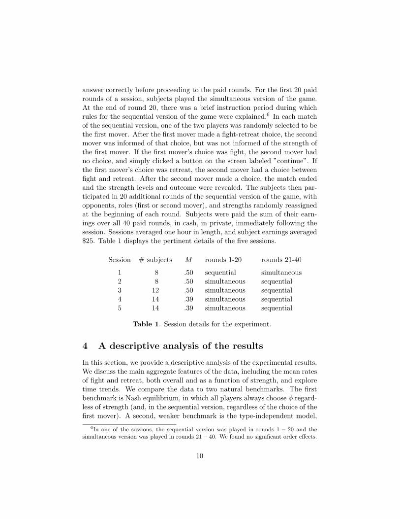
answer correctly before proceeding to the paid rounds. For the first 20 paidrounds of a session, subjects played the simultaneous version of the game.At the end of round 20, there was a brief instruction period during whichrules for the sequential version of the game were explained.6 In each matchof the sequential version, one of the two players was randomly selected to bethe first mover. After the first mover made a fight-retreat choice, the secondmover was informed of that choice, but was not informed of the strength ofthe first mover. If the first mover’s choice was fight, the second mover hadno choice, and simply clicked a button on the screen labeled ”continue”. Ifthe first mover’s choice was retreat, the second mover had a choice betweenfight and retreat. After the second mover made a choice, the match endedand the strength levels and outcome were revealed. The subjects then par-ticipated in 20 additional rounds of the sequential version of the game, withopponents, roles (first or second mover), and strengths randomly reassignedat the beginning of each round. Subjects were paid the sum of their earn-ings over all 40 paid rounds, in cash, in private, immediately following thesession. Sessions averaged one hour in length, and subject earnings averaged$25. Table 1 displays the pertinent details of the five sessions.

Session # subjects M rounds 1-20 rounds 21-40

1 8 .50 sequential simultaneous2 8 .50 simultaneous sequential3 12 .50 simultaneous sequential4 14 .39 simultaneous sequential5 14 .39 simultaneous sequential

Table 1. Session details for the experiment.

4 A descriptive analysis of the results

In this section, we provide a descriptive analysis of the experimental results.We discuss the main aggregate features of the data, including the mean ratesof fight and retreat, both overall and as a function of strength, and exploretime trends. We compare the data to two natural benchmarks. The firstbenchmark is Nash equilibrium, in which all players always choose φ regard-less of strength (and, in the sequential version, regardless of the choice of thefirst mover). A second, weaker benchmark is the type-independent model,

6In one of the sessions, the sequential version was played in rounds 1 − 20 and thesimultaneous version was played in rounds 21− 40. We found no significant order effects.

10

where the probability of fighting is independent of strength. We study thedifferences in probabilities of fighting as a function of the compromise pay-off and the timing of the game. Last, we analyze the data at an individuallevel. For each player, we estimate a decision rule that maps strength intoa probability of fighting.

4.1 Aggregate fight rates unconditional on strength

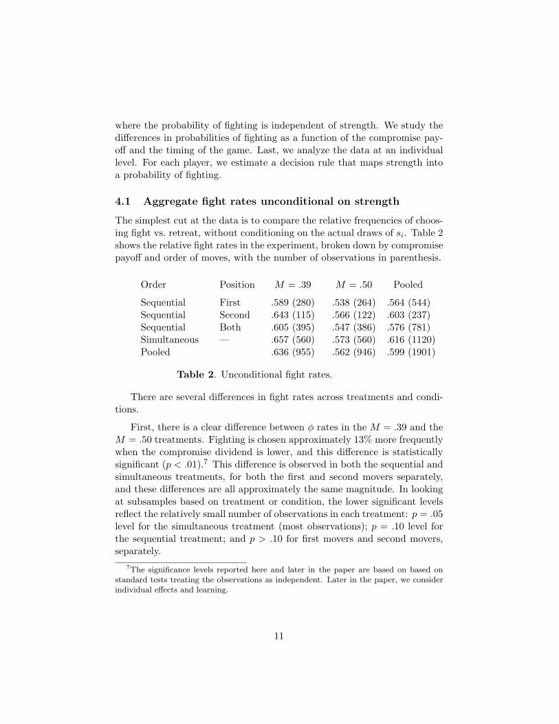
The simplest cut at the data is to compare the relative frequencies of choos-ing fight vs. retreat, without conditioning on the actual draws of si. Table 2shows the relative fight rates in the experiment, broken down by compromisepayoff and order of moves, with the number of observations in parenthesis.

Order Position M = .39 M = .50 Pooled

Sequential First .589 (280) .538 (264) .564 (544)Sequential Second .643 (115) .566 (122) .603 (237)Sequential Both .605 (395) .547 (386) .576 (781)Simultaneous — .657 (560) .573 (560) .616 (1120)Pooled .636 (955) .562 (946) .599 (1901)

Table 2. Unconditional fight rates.

There are several differences in fight rates across treatments and condi-tions.

First, there is a clear difference between φ rates in the M = .39 and theM = .50 treatments. Fighting is chosen approximately 13% more frequentlywhen the compromise dividend is lower, and this difference is statisticallysignificant (p < .01).7 This difference is observed in both the sequential andsimultaneous treatments, for both the first and second movers separately,and these differences are all approximately the same magnitude. In lookingat subsamples based on treatment or condition, the lower significant levelsreflect the relatively small number of observations in each treatment: p = .05level for the simultaneous treatment (most observations); p = .10 level forthe sequential treatment; and p > .10 for first movers and second movers,separately.

7The significance levels reported here and later in the paper are based on based onstandard tests treating the observations as independent. Later in the paper, we considerindividual effects and learning.

11

Second, first movers in the sequential game fight less frequently thansecond movers, both in the .39 and the .50 treatments. The differences inmeans are not statistically significant.

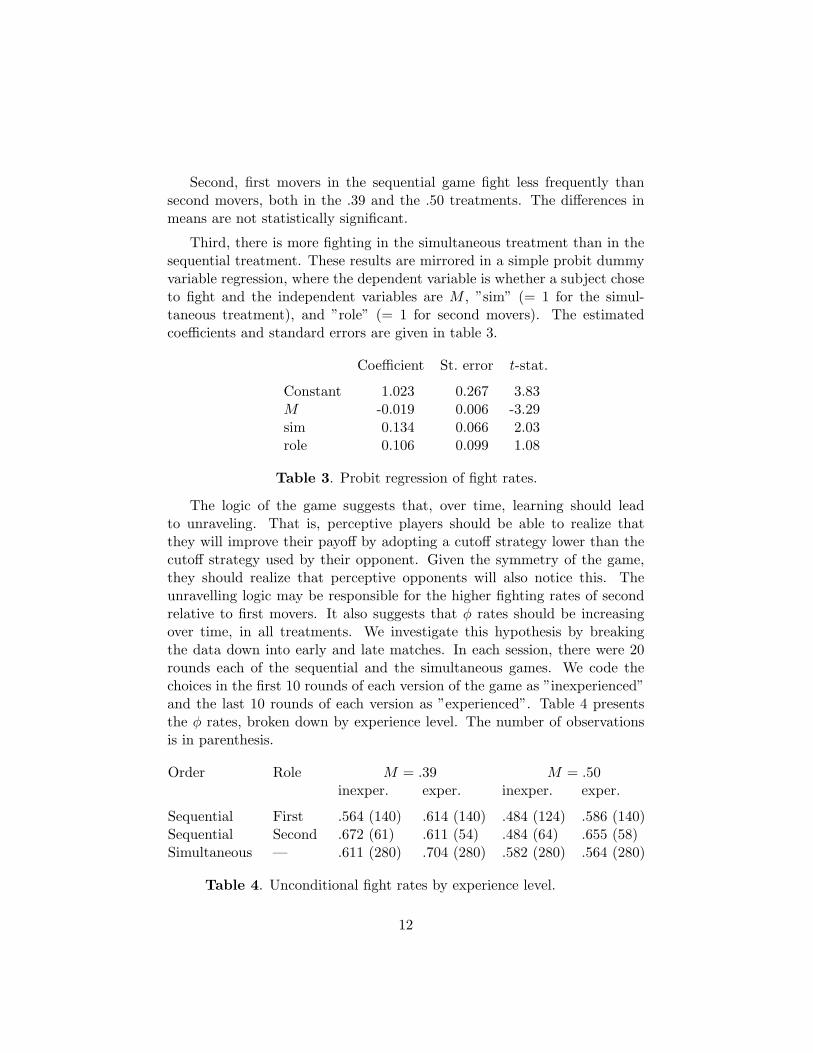
Third, there is more fighting in the simultaneous treatment than in thesequential treatment. These results are mirrored in a simple probit dummyvariable regression, where the dependent variable is whether a subject choseto fight and the independent variables are M , ”sim” (= 1 for the simul-taneous treatment), and ”role” (= 1 for second movers). The estimatedcoefficients and standard errors are given in table 3.

Coefficient St. error t-stat.

Constant 1.023 0.267 3.83M -0.019 0.006 -3.29sim 0.134 0.066 2.03role 0.106 0.099 1.08

Table 3. Probit regression of fight rates.

The logic of the game suggests that, over time, learning should leadto unraveling. That is, perceptive players should be able to realize thatthey will improve their payoff by adopting a cutoff strategy lower than thecutoff strategy used by their opponent. Given the symmetry of the game,they should realize that perceptive opponents will also notice this. Theunravelling logic may be responsible for the higher fighting rates of secondrelative to first movers. It also suggests that φ rates should be increasingover time, in all treatments. We investigate this hypothesis by breakingthe data down into early and late matches. In each session, there were 20rounds each of the sequential and the simultaneous games. We code thechoices in the first 10 rounds of each version of the game as ”inexperienced”and the last 10 rounds of each version as ”experienced”. Table 4 presentsthe φ rates, broken down by experience level. The number of observationsis in parenthesis.

Order Role M = .39 M = .50inexper. exper. inexper. exper.

Sequential First .564 (140) .614 (140) .484 (124) .586 (140)Sequential Second .672 (61) .611 (54) .484 (64) .655 (58)Simultaneous — .611 (280) .704 (280) .582 (280) .564 (280)

Table 4. Unconditional fight rates by experience level.

12

The effects of experience on the unconditional φ rates is ambiguous. Infour of the six comparisons, the φ rate increases, as hypothesized, althoughit remains well below 1. All four such differences are statistically significant.In two of the six comparisons, φ decreases, but these two changes are notsignificant. Furthermore, the two treatments where φ decreases have noapparent relation with each other (simultaneous with M = .50 and secondplayer in sequential with M = .39).

4.2 Aggregate fight rates conditional on strength

The analysis above, while providing a useful sketch of the results, falls shortof giving a complete picture of the aggregate data, because the uncondi-tional φ rates are not a sufficient statistic for the actual strategies. A be-havior strategy in each game is a probability of choosing φ conditional ons. By aggregating across all the (strength, action) paired observations for atreatment, we can graphically display the aggregate empirical behavior strat-egy, and then compare this strategy across treatments. Figure 1 shows sixgraphs. The graphs on the left correspond to M = .39, and the graphs onthe right are for M = .50. The middle and bottom graphs are for the firstand second movers in the sequential treatment, and the top graphs for thesimultaneous movers. The strength is on the horizontal axis, on a scale of0 to 100, and the empirical fighting frequencies are on the vertical axis ona scale of 0 to 1. Thus, for example, if all subjects were to choose the samecutoff strategy s∗, then we would observe a step function, with a probabilityof fighting equal to 0 below s∗ and equal to 1 above s∗. Note that func-tions need not be monotonically increasing, although we expect that playerswith higher strength will be more likely to fight. The empirical frequenciesare aggregated into bins of 5 units of strength (1-5, 6-10, etc.) along thehorizontal axis, with φ-probabilities in the vertical axis.

[ Figure 1 here ]

These graphs suggest that second movers in the sequential version ofthe game behave differently from first movers in at least two ways. Secondmovers fight more than first movers. If one looks at the point in the graphwhere the fight probabilities first reach 50%, this switchpoint is in the high20s for second movers in both the .39 and .50 treatments, while it is in themid to high 30s for simultaneous movers and even higher for the first moversin the sequential treatment. These results are also supported by a probitregression similar to the one reported in table 3, but including the indepen-dent variable s to control for strength. The coefficients and t-statistics are

13

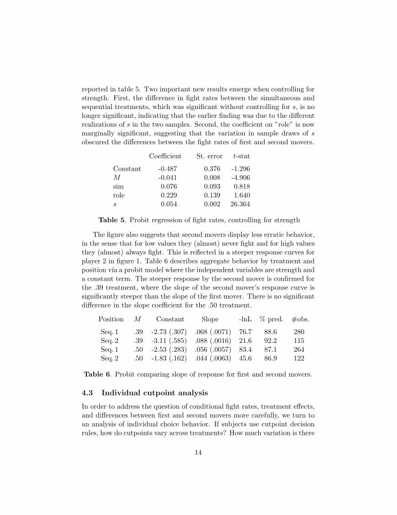
reported in table 5. Two important new results emerge when controlling forstrength. First, the difference in fight rates between the simultaneous andsequential treatments, which was significant without controlling for s, is nolonger significant, indicating that the earlier finding was due to the differentrealizations of s in the two samples. Second, the coefficient on ”role” is nowmarginally significant, suggesting that the variation in sample draws of sobscured the differences between the fight rates of first and second movers.

Coefficient St. error t-stat

Constant -0.487 0.376 -1.296M -0.041 0.008 -4.906sim 0.076 0.093 0.818role 0.229 0.139 1.640s 0.054 0.002 26.364

Table 5. Probit regression of fight rates, controlling for strength

The figure also suggests that second movers display less erratic behavior,in the sense that for low values they (almost) never fight and for high valuesthey (almost) always fight. This is reflected in a steeper response curves forplayer 2 in figure 1. Table 6 describes aggregate behavior by treatment andposition vıa a probit model where the independent variables are strength anda constant term. The steeper response by the second mover is confirmed forthe .39 treatment, where the slope of the second mover’s response curve issignificantly steeper than the slope of the first mover. There is no significantdifference in the slope coefficient for the .50 treatment.

Position M Constant Slope -lnL % pred. #obs.

Seq. 1 .39 -2.73 (.307) .068 (.0071) 76.7 88.6 280Seq. 2 .39 -3.11 (.585) .088 (.0016) 21.6 92.2 115Seq. 1 .50 -2.53 (.283) .056 (.0057) 83.4 87.1 264Seq. 2 .50 -1.83 (.162) .044 (.0063) 45.6 86.9 122

Table 6. Probit comparing slope of response for first and second movers.

4.3 Individual cutpoint analysis

In order to address the question of conditional fight rates, treatment effects,and differences between first and second movers more carefully, we turn toan analysis of individual choice behavior. If subjects use cutpoint decisionrules, how do cutpoints vary across treatments? How much variation is there

14

across individuals? How consistent is individual behavior with cutpoint de-cision rules? We document that there is some heterogeneity across subjects,but more importantly, the distribution of these cutpoint strategies variessystematically across treatments.

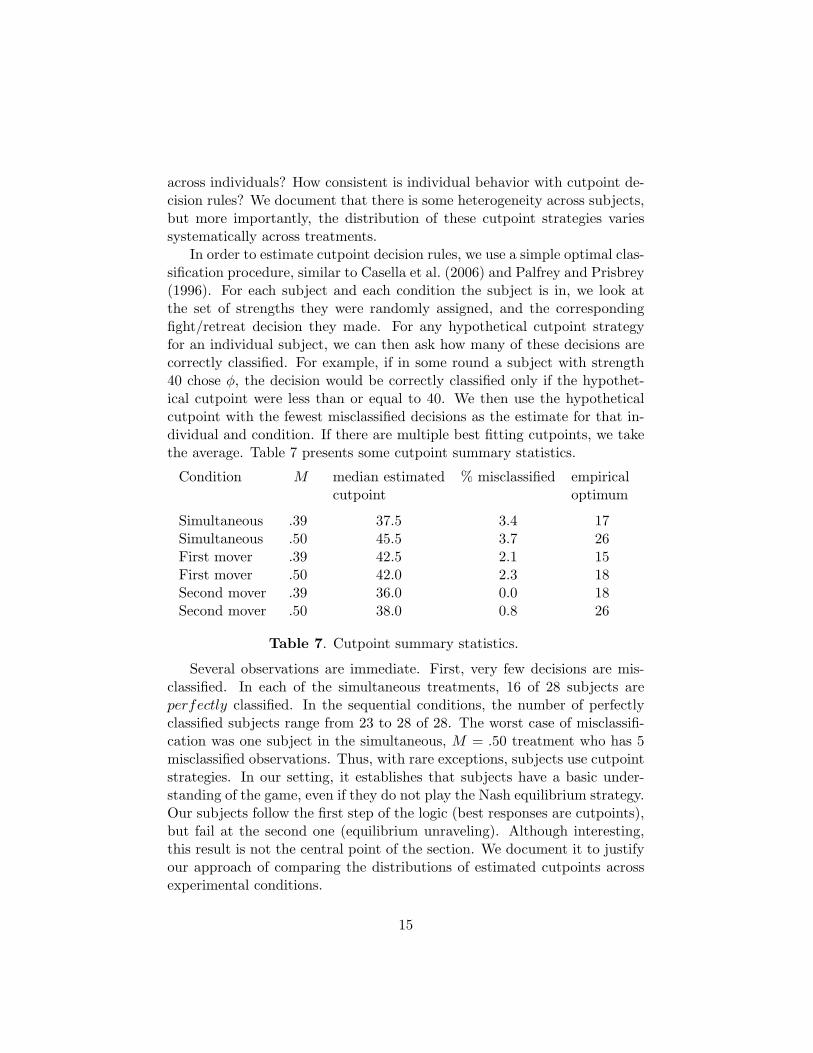
In order to estimate cutpoint decision rules, we use a simple optimal clas-sification procedure, similar to Casella et al. (2006) and Palfrey and Prisbrey(1996). For each subject and each condition the subject is in, we look atthe set of strengths they were randomly assigned, and the correspondingfight/retreat decision they made. For any hypothetical cutpoint strategyfor an individual subject, we can then ask how many of these decisions arecorrectly classified. For example, if in some round a subject with strength40 chose φ, the decision would be correctly classified only if the hypothet-ical cutpoint were less than or equal to 40. We then use the hypotheticalcutpoint with the fewest misclassified decisions as the estimate for that in-dividual and condition. If there are multiple best fitting cutpoints, we takethe average. Table 7 presents some cutpoint summary statistics.

Condition M median estimated % misclassified empiricalcutpoint optimum

Simultaneous .39 37.5 3.4 17Simultaneous .50 45.5 3.7 26First mover .39 42.5 2.1 15First mover .50 42.0 2.3 18Second mover .39 36.0 0.0 18Second mover .50 38.0 0.8 26

Table 7. Cutpoint summary statistics.

Several observations are immediate. First, very few decisions are mis-classified. In each of the simultaneous treatments, 16 of 28 subjects areperfectly classified. In the sequential conditions, the number of perfectlyclassified subjects range from 23 to 28 of 28. The worst case of misclassifi-cation was one subject in the simultaneous, M = .50 treatment who has 5misclassified observations. Thus, with rare exceptions, subjects use cutpointstrategies. In our setting, it establishes that subjects have a basic under-standing of the game, even if they do not play the Nash equilibrium strategy.Our subjects follow the first step of the logic (best responses are cutpoints),but fail at the second one (equilibrium unraveling). Although interesting,this result is not the central point of the section. We document it to justifyour approach of comparing the distributions of estimated cutpoints acrossexperimental conditions.

15

The key questions concern whether the distribution of cutpoints variessystematically across treatments and, in the sequential games, between firstand second movers. We also want to understand whether these systematicvariations are consistent with the descriptive findings based on aggregatedata described in the previous section. Table 7 reports the median estimatedcutpoint across all subjects, and the percentage of misclassified decisions,by condition. The median cutpoints mirror the aggregate fight rates bytreatment and condition, as reported in previous sections. Cutpoints arelower (more fighting) in M = .39 than in M = .50 treatments. They arelower for second movers than first movers for both the M = .39 and M = .50treatments, and they are also lower for second movers than for players inthe simultaneous condition for both the M = .39 and M = .50 treatments.There is no systematic difference between first movers and players in thesimultaneous condition. Last, second movers have fewer classification errors(therefore, steeper response curves) than first movers.

As further evidence, we consider how the entire distribution of indi-vidual estimated cutpoints varies across treatments. Figure 2 displays theestimated cumulative frequency distribution of individual cutpoints used byour subjects for all the treatments, and broken down by position in the se-quential treatment. The horizontal axis represents cutpoints, ranging from0 to 100. The vertical axis indicates how many of the subjects in each treat-ment or position (out of 28) were using a cutpoint less than or equal to thatnumber.

[ Figure 2 here ]

These distributions exhibit a wide range of estimated cutpoints, withfew above 60 or below 20. In all treatments and conditions, there is het-erogeneity that is both significant (one easily rejects the hypothesis that allsubjects use the same cutpoint for any of these conditions), and substan-tial. The distributions are also different across treatments and conditions.Also noteworthy is that distributions are never concentrated around partic-ular cutpoints (i.e., step distribution functions), but they are smoothly anduniformly increasing over the range.

Finally, one can compare the distribution of cutpoints used by players inthe game to the cutpoint that would be optimal, given the actual frequenciesof fighting in the experiment. These ”empirically optimal” cutpoints aregiven in the last column of table 7. The optimal cutpoints are generallyabout one-half times the corresponding median estimated cutpoints. Many,but not all, players are ”fooled” by this game, in the sense that they set

16

cutpoints that are too high. We find that 20% of the estimated cutpointsare within 5 units of strength of the optimal cutpoint, and these subjectsare leaving essentially no money on the table. Of the remaining estimatedcutpoints, 7% are below the optimal cutpoint by at least 5 strength units,and 73% are above the optimal cutpoint by at least 5 units.

4.4 Summary of descriptive analysis

The main findings of our analysis so far can be summarized as follows.

• Unconditional fight rates range from about 50% to 70%, dependingon the treatment and condition, falling far short of the theoreticalprediction of 100%.

• In all treatments, the φ-rate conditional on strength increases monoton-ically from virtually 0% for strengths below 20 to virtually 100% forstrengths above 60 if M = .39 or above 70 if M = .50.

• The compromise payoff, M , affects behavior, with less fighting whenthe compromise payoff is higher.

• There are some differences between the sequential and simultaneoustreatments. Most striking is that second movers behave differentlythan first movers: the former display more fighting and less erraticbehavior (when M = .39) than the latter. For a theory to explainthis pattern, it must predict that observing the behavior of the rivalbefore making inferences and choices leads to systematic differencescompared with just conditioning on a hypothetical event.

• We do not find consistent evidence of learning. A possible explanationis the insufficient feedback provided to players (only the rival’s strengthand outcome is revealed at the end of each round). However, giventhat the order of moves matters, one would expect that second moverswould use their experience in that role when they subsequently playas first mover.8

• The vast majority of subjects use cutpoint strategies, with very fewdeviations. Across all treatments, over 97% of individual behavior is

8Recall that, in our design, all players gain experience as both first and second movers.That is, our data on first and second movers are all coming from the same subjects.Subjects apparently do not draw inferences from their own decision making in differentroles about how other subjects behave in those roles.

17

consistent with cutpoint strategies. This shows their understanding, atleast at an intuitive level, that the expected payoff differential betweenφ and ρ increases with s, and possibly an even deeper understandingthat the best reply in this game is always a cutpoint strategy. It alsojustifies the analysis that focuses on estimated cutpoints.

• The distribution of these cutpoints varies by condition in ways thatmirror the differences in the aggregate fight rates. The empirical dis-tribution of individual cutpoints is smooth.

5 Alternative behavioral models

Obviously, the Nash equilibrium model is inconsistent with our data. In thissection, we consider several alternative models to explain the excessivelylow fight rates. Note that this game is easily solved by iterated dominance,but only using weak rather than strict dominance. Denote a strategy as afunction that maps strength into a probability of fighting q : [0, 1] → [0, 1].First note that any strategy q that assigns q(1) < 1 is weakly dominatedby the strategy q′ where q′(s) = q(s) for all s 6= 1 and q′(1) = 1. In theexperiments, the type distribution was discrete, so once we eliminate allthose strategies, then any strategy q that assigns q(.99) < 1 and q(1) = 1 isweakly dominated by the strategy q′ where q′(s) = q(s) for all s 6= .99 andq′(.99) = 1. And so forth.9 On the other hand, rationalizability does noteliminate any strategy, since every strategy is a weak best response to theequilibrium strategy, q∗(s) = 1 for all s.

We consider two categories of models. Models in the first category havetheir foundations in cognitive limitations, and they all have features thatadmit the possibility of observing weakly dominated strategies. We studythree models within this class: quantal response equilibrium or QRE (McK-elvey and Palfrey, 1995), cognitive hierarchy or CH (Camerer et al., 2004),and cursed equilibrium or CE (Eyster and Rabin, 2005).10 We also considersome variations that allow for heterogeneity or hybridization between mod-els, such as the truncated quantal response equilibrium or TQRE (Camerer

9For the M = .50 game, at the last iteration, a player with the lowest strength, s = .01,is indifferent between φ and ρ, and therefore, there is an equilibrium with s = .01 typeschoosing ρ and all other types choosing φ. For the M = .39 game, the iteration continuesall the way down, and the only equilibrium is q∗(s) = 1 for all s.

10Some preliminary findings about CH and CE are discussed in Wang (2006), withpermission of the authors.

18

et al., 2006). These hybrid versions allow us to understand better how dif-ferent models capture different features of the observed behavior. Models inthe second category have their foundations on the existence of systematic de-viations from self-interest : social preferences, fairness motives, reciprocity,or altruism. For reasons we discuss later, we estimate only models in thefirst category.

5.1 Quantal Response Equilibrium

Quantal response equilibrium applies stochastic choice theory to strategicgames. It is motivated by the idea that a decision maker may take a sub-optimal action, and the probability of doing so is increasing in the expectedpayoff of the action. In a regular QRE (Goeree et al., 2005), one simplyreplaces the best response correspondence used to characterize Nash equi-librium, with a quantal response function that is continuous and monotonein expected payoffs. That is, the probability of choosing a strategy is acontinuous increasing function of the expected payoff of using that strategy,and strategies with higher payoffs are used with higher probability thanstrategies with lower payoffs. A quantal response equilibrium is then a fixedpoint of the quantal response mapping. In a logit equilibrium, for any twostrategies, the log odds of the choice probabilities are proportional to the dif-ference in expected payoffs, where the proportionality factor, λ, is a measureof responsiveness of choices to payoffs. That is:

ln[

σij

σik

]= λ

[Uij − Uik

]where σij is the probability that player i chooses strategy j, and Uij is thecorresponding expected payoff in equilibrium. Note that a higher λ reflects a”more precise” response to the payoff differential. The polar cases λ = 0 andλ → +∞ correspond to random choice and Nash equilibrium, respectively.

Specification of the QRE model. We consider two different specifica-tions of the logit equilibrium version of QRE. The first specification takesan interim approach and analyzes the game in behavioral strategies. Thisapproach corresponds to the agent QRE (AQRE) of McKelvey and Palfrey(1998). Conditional on player 1’s strength, and given the AQRE behavioralstrategies used by player 2, the log-odds of player 1 choosing retreat vs.fight is proportional to the difference in expected payoffs between retreatand fight – and similarly for player 2.

19

The second analyzes the game in ex ante strategies, and assumes playerschoose stochastically over possible plans for whether or not to fight as afunction of strength. Because the set of all possible pure strategies in ourgame is huge (2100), we are forced to consider only a subset of such strate-gies. The natural restriction is to consider only monotone strategies, i.e.,cutpoint strategies. This is a natural criterion since monotone strategiesare always best responses and, furthermore, any non-monotone strategy isweakly dominated by a monotone strategy. This also reduces the set ofpure strategies to a small enough number (100) that estimation is possible.Last, focusing on cutpoint strategies does not seem too restrictive, giventhat the behavior of individuals is highly consistent with this type of play,as previously documented.

In the logit parameterization of the cutpoint QRE, the distribution overcutpoint strategies used by player 2 has the standard property. Namely, thelog-odds of player 1 choosing any cutpoint c versus any other cutpoint c′

is proportional to the ex ante difference in expected payoffs between usingthose two cutpoints – and similarly for player 2.

Logit QRE in behavioral strategies. For any response parameter λwe solve for a fixed point in behavioral strategies. Denote by φ∗λ such anequilibrium fixed point, and by φ∗λ(s) the equilibrium probability of fightinggiven a strength s.

Consider first the simultaneous game. We need to determine the ex-pected utility of φ for a player with strength s conditional on the otherplayer using strategy φ∗λ and having chosen ρ. This is simply equal to theconditional probability that the other player has strength less than s, giventhat he has chosen ρ. It is then given by:

Vφ(s;φ∗λ) =

∫ s0 [1− φ∗λ(t)]dt∫ 10 [1− φ∗λ(t)]dt

(1)

The expected utility of ρ conditional on the other player having chosen ρ issimply Vρ(s;φ∗λ) = M , so the difference in the expected utility of φ and ρ is:

∆(s;φ∗λ) =∫ 1

0[1− φ∗λ(t)]dt

(Vφ(s;φ∗λ)− Vρ(s;φ∗λ)

)=

∫ s

0[1− φ∗λ(t)]dt−M

∫ 1

0[1− φ∗λ(t)]dt

Hence, in a symmetric logit QRE, φ∗λ is characterized by:

20

φ∗λ(s) =eλ∆(s;φ∗λ)

1 + eλ∆(s;φ∗λ)for all s ∈ [0, 1]

The sequential game requires solving simultaneously for φ∗λ1(s1) andφ∗λ2(s2). The expressions for the first mover are exactly the same as inthe simultaneous move game. Therefore, modifying the notation slightly tomake clear that it is player 1’s equation, we get:

φ∗λ1(s1) =eλ∆1(s1;φ∗λ2)

1 + eλ∆1(s1;φ∗λ2)for all s1 ∈ [0, 1]

where

∆1(s1;φ∗λ2) =∫ s1

0[1− φ∗λ2(t)]dt−M

∫ 1

0[1− φ∗λ2(t)]dt

The condition for the second mover is the same, except the second mover’sexpected utility difference does not have to be conditioned on the first moverchoosing ρ. We get:

φ∗λ2(s2) =eλ∆2(s2;φ∗λ1)

1 + eλ∆2(s2;φ∗λ1)for all s2 ∈ [0, 1]

where

∆2(s2;φ∗λ1) =

∫ s2

0 [1− φ∗λ1(t)]dt∫ 10 [1− φ∗λ1(t)]dt

−M

Logit QRE in cutpoint strategies. We next consider the slightly moresophisticated version of QRE where players are assumed to randomize overmonotone cutpoint strategies, which we call QRE-cut. In our game, a cut-point strategy is a critical value of strength, c, such that player i chooses φ ifsi ≥ c and chooses ρ if si < c. Hence, we define a cutpoint quantal responseto be given by two probability distributions over c, one for each player, de-noted q1(c) and q2(c). In the simultaneous version of the game, we consideronly symmetric QRE-cut, where q1(c) = q2(c) = q(c) for all c. For the se-quential version, generally q1(c) 6= q2(c), since it is not a symmetric gameand the second player chooses a cutpoint after observing the first player’smove. We use the logit quantal response function for a parametric specifi-cation. Hence, the probability that a player chooses a particular strategyis proportional to the exponentiated expected payoff from using that strat-egy, given the cutpoint quantal response function of the other player. It isworth noting that past studies have found that in binary choice games with

21

continuous types, a cutpoint strategy can be a useful variation on the stan-dard QRE approach (see Casella et al., 2006). Furthermore, the analysis insection 4.3 suggests that subjects adhere to this type of strategies.

Consider the simultaneous game. The expected utility to player 1 ofusing a cutpoint strategy c if player 2 uses q(·) is given by:

U(c) =∫ 1

csds +

∫ c

0

[∫ s

0q(c) (cM + (s− c)) dc +

∫ 1

sq(c)cMdc

]ds (2)

The first term is the probability of drawing a strength s above the cutpoint,in which case player 1 chooses φ and obtains a payoff 1 only if player 2 hasa lower strength. The second term is the probability of drawing a strengths below the cutpoint, in which case player 1 chooses ρ. Then, if player 2’sstrength is lower, a compromise gives payoff M and a no-compromise givespayoff 1. If player 2’s strength is higher, a compromise gives payoff M anda no-compromise gives payoff 0. In a symmetric logit QRE-cut:

q(c) =eλU(c)∫ 1

0 eλU(c)dcfor all c ∈ [0, 1]

In the sequential game, the expression for the first mover’s utility ofusing c, given player 2 uses q2(·) is the same as in the simultaneous case:

U1(c) =∫ 1

cs1ds1 +

∫ c

0

[∫ s1

0q2(c) (cM + (s1 − c)) dc +

∫ 1

s1

q2(c)cMdc

]ds1

(3)By contrast, the second mover’s utility of using c, given player 1 uses q1(·)does not have to be conditioned on the first mover choosing ρ. That is:

U2(c) =∫ 1

c

[∫ s2

0 c1q1(c1)dc1∫ 10 c1q1(c1)dc1

+

∫ 1s2

s2q1(c1)dc1∫ 10 c1q1(c1)dc1

]ds2 + cM (4)

There are three observations to make about the QRE-cut solutions.First, in the sequential game, the equilibrium cutpoint distributions aredifferent for the two players. The second mover generally adopts lower cut-points, which translates into higher φ rates. Second, players adopt lowercutpoints when M is lower. Third, the cutpoint distributions for the firstmover in the sequential games are different from the cutpoint distributionsin the corresponding simultaneous games, even though the utility formulas(equations 2 and 3) are identical.

22

We fit the behavioral strategy logit QRE and the cutpoint strategy logitQRE models by standard maximum likelihood techniques, i.e., finding thevalue of λ that maximizes likelihood of the observed frequencies of strategies.We estimate restricted and unrestricted versions of the models. In the mostrestricted version, the parameters are constrained to be the same across alltreatments. We also estimate a version where the parameters are constrainedto be the same for the .39 and .50 treatments, but are allowed to be differentin the simultaneous and sequential games.

5.2 Cognitive Hierarchy

The cognitive hierarchy model (Camerer et al., 2004) postulates that whena player makes a choice, his decision process corresponds to a ”level of so-phistication” k with probability pk. The CH solution to a game is uniquelydetermined by an assumption about how level 0 types behave (σ0), and thedistribution of levels of sophistication (p).11 Once the behavior of level 0players is determined, level 1 players are characterized by choosing withequal probability all strategies that are best responses to level 0 opponents.Level 2 players optimize assuming they face a distribution of level 0 andlevel 1 players, where the distribution satisfies truncated rational expecta-tions. That is, the beliefs of level 2 players that their opponent is choosingaccording to a level 0 or a level 1 decision process, denoted b2(0) and b2(1),is given by the truncated ”true” distribution of these types: b2(0) = p0

p0+p1

and b2(1) = p1

p0+p1. Level 2 players are then characterized by choosing with

equal probability all strategies that are best responses to b2 beliefs aboutthe opponents. Higher levels are defined analogously, so a level k optimizeswith respect to beliefs bk where bk(j) = pj/

∑k−1l=0 pl for all j ∈ {1, ..., k−1}.

For any distribution of levels, p, this implies a unique specification ofa mixed strategy for each level, σ(p) = (σ0(p), ..., σk(p), ...), and this spec-ification can be solved recursively, starting with the lowest types. Thisgenerates predictions about the aggregate distribution of actions, denotedσ(p) =

∑∞k=0 pkσk(p). In all applications to date, p is assumed to be Poisson

distributed with mean τ . That is, pk = τk

k! e−τ . We consider two specifica-

tions of the behavior of level 0 types.11The CH model is an extension of the original level-k model of Nagel (1995). See Stahl

and Wilson (1995), Crawford and Iriberri (2005), Costa-Gomes and Crawford (2006),and Camerer et al. (2006) for further examples of estimation of level-k models, based onexperimental data.

23

Random actions. In the standard CH model, level 0 players are typicallyassumed to choose an action randomly. In the context of our game, thismeans that they are equally likely to select φ or ρ, independently of theirstrength. Level 1 types best respond to level 0 types. It can be easily shownthat the best response strategy is to choose cutpoint M . Level 2 playersthen optimize with a cutpoint somewhere between M (the best response ifeveryone is level 0) and M2 (the best response if everyone is level 1), withthe exact value depending on p0 and p1. Behavior by higher level players isdefined recursively.

Random cutpoints. An alternative version, which we call the cutpointcognitive hierarchy model or CH-cut, replaces the assumption that level0 types randomize uniformly over actions, with the assumption that theyrandomize uniformly over cutpoint strategies. This implicitly endows level0 types with some amount of rationality, in the form of monotone behavior:they are more likely to choose φ when their strength is high than whentheir strength is low. In our game, a level 0 type who randomizes overcutpoints has a probability of fighting as a function of s which is equal tos. As in the standard CH, the best responses of higher types will be uniquecutpoints, and are easily calculated by recursion. Since a level 0 type has aprobability 1−s of choosing ρ, the posterior distribution of strength of a level0 type conditional on choosing ρ is f(s | ρ) = 1−sR 1

0 (1−x)dx= 2− 2s. Hence, the

expected payoff of φ for a level 1 type with strength s and conditional on theother player being level 0 and choosing ρ is

∫ s0 (2−2x)dx = 2s−s2. Since the

payoff of ρ is M , the optimal cutpoint of a level 1 type is the value sM1 that

solves 2sM1 −(sM

1 )2 = M , that is sM1 = 1−

√1−M . For our two treatments,

we get s.501 = 1−

√1/2 ≈ .29 and s.39

1 = 1−√

11/18 ≈ .22. Higher types arethen defined recursively, with the exact cutpoint for a level k depending on{pl}k−1

l=0 . This produces a CH model that is comparable to QRE in the sensethat all players choose cutpoint strategies, so φ probabilities are monotonein s for all players.

We fit the Poisson specification of the CH and cutpoint CH models to thedata set by finding the value of τ that maximizes likelihood of the observedaggregate frequencies of strategies, under the assumption that types areidentically and independently distributed draws. We estimate the best-fitting values of τ by maximum likelihood for each of the four treatments,and report both constrained and unconstrained estimates.

24

5.3 Combining quantal response and strategic hierarchies(TQRE)

The predictions of the CH and CH-cut models differ from the QRE andQRE-cut models in two important ways. First, in CH models, all playerswith the same level of sophistication choose the same cutpoint strategy.Second, predictions in CH are identical for the sequential and simultaneousversions of the game. Neither ”bunching” by layers of reasoning nor identicalbehavior in the simultaneous and sequential treatments are observed in thedata.

An approach that combines quantal response and hierarchical thinking,called Truncated Quantal Response Equilibrium (TQRE), is developed inCamerer et al. (2006). This model introduces a countable number of players’skill levels, λ0, λ1, ..., λk, ... . The distribution of skill levels in the populationis given by p0, p1, ..., pk, ... . A player with skill level k chooses stochasticallywith a logit quantal response function with precision λk. TQRE assumestruncated rational expectations in a similar manner to CH: a player withprecision λk has beliefs pk

j = pj/∑k−1

l=0 pl for j < k and pkj = 0 for j ≥ k.

For reasons of parsimony and comparability to CH, we assume that skilllevels are Poisson distributed and equally space λk = γk. Thus, it is a twoparameter model with Poisson parameter, τ , and a spacing parameter, γ.

The TQRE model has two effects. It smooths out the mass points, andit makes different predictions for the sequential and simultaneous games.These effects work slightly differently with behavioral strategies and withcutpoint strategies, so we estimate both versions.

5.4 Cursed Equilibrium

In a CE model, players are assumed to systematically underestimate thecorrelation between the opponents’ action and information. As in the CHmodel, a cursed equilibrium will be the same in both the sequential andsimultaneous treatments. In an α-cursed equilibrium (CEα) all players areα-cursed. However, players believe that opponents are α-cursed with prob-ability (1 − α) and they believe that actions of opponents are independentof their information with probability α. All players optimize with respectto this (incorrect) mutually held belief about the joint distribution of op-ponents’ actions and information. In our model, we can easily compute thecutpoint strategy in CEα as a function of M , denoted s∗α(M). For a playerwith strength si, and assuming the other player is using s∗α(M), the expected

25

utility of φ, conditional on the opponent choosing ρ is given by:

V αφ (si) = α Pr{sj < si}+ (1− α) Pr{sj < si | aj = ρ, s∗α(M)}

= αsi + (1− α) min{1, sis∗α(M)}

A player with strength equal to the equilibrium cutpoint must be indifferentbetween φ and ρ. Formally, V α

φ (s∗α(M)) = V αρ (s∗α(M)). Therefore:12

s∗α(M) =

{1− 1−M

α if α > 1−M

0 if α ≤ 1−M

A difficulty with CEα is that it cannot be fit to the data due to a zero-likelihood problem: for each α it makes a point prediction. Therefore,we slightly modify the equilibrium concept in order to allow for stochas-tic choice. The approach we follow is to combine QRE with CEα.13 In thesimultaneous move game, a (symmetric) α-QRE is a behavior strategy, or aset of probabilities of choosing φ, one for each value of s ∈ [0, 1]. We denotesuch a strategy evaluated at a specific strength value by φ(s). Given λ and αwe denote by α-QRE the behavior strategy φ∗λα. If player j is using φ∗λα andplayer i is α-cursed, then i’s expected payoff from choosing φ when si = sis given by:

V αφ (s) =

∫ 1

0φ∗λα(t)dt

[αs + (1− α) Pr{sj < s | aj = φ, φ∗λα}

]+

∫ 1

0[1− φ∗λα(t)]dt

[αs + (1− α) Pr{sj < s | aj = ρ, φ∗λα}

]= αs

∫ 1

0φ∗λα(t)dt + (1− α)

∫ s

0φ∗λα(t)dt

+αs

∫ 1

0[1− φ∗λα(t)]dt + (1− α)

∫ s

0[1− φ∗λα(t)]dt

And the expected payoff from choosing ρ is:

V αρ (s) = αs

∫ 1

0φ∗λα(t)dt + (1− α)

∫ s

0φ∗λα(t)dt + M

∫ 1

0[1− φ∗λα(t)]dt

12In a fully cursed equilibrium (α = 1), all players choose strategies as if there is nocorrelation between the opponent’s action and information. Thus, they all behave like alevel 1 player in CH with random actions: s∗1(M) = M .

13Note that player heterogeneity with respect to α would not solve the zero-likelihoodproblem: for any cursedness α ∈ [0, 1], it is always true that s∗α(M) ≤ M . However, inour data set, we have many observations where players with strength s > M choose ρ.

26

Using the logit specification for the quantal response function, we then applylogit choice probabilities to the difference in the expected payoff from φ andρ for each si = s. By inspection of V α

φ (s) and V αρ (s), this difference is:

∆(s;φ∗λα) = αs

∫ 1

0[1−φ∗λα(t)]dt+(1−α)

∫ s

0[1−φ∗λα(t)]dt−M

∫ 1

0[1−φ∗λα(t)]dt

and the α-QRE in the simultaneous game is then characterized by:

φ∗λα(s) =eλ∆(s;φ∗λα)

1 + eλ∆(s;φ∗λα)for all s ∈ [0, 1]

which can be solved numerically, for any value of α.

In the sequential version of the game, we need to simultaneously solvefor the first and second movers, φ∗λα1 and φ∗λα2, respectively. The expectedpayoff equations under φ and ρ for the first mover are the same as in thesimultaneous move game, so we have:

V αφ1(s1) = αs1

∫ 1

0φ∗λα2(s2)ds2 + (1− α)

∫ s1

0φ∗λα2(s2)ds2

+αs1

∫ 1

0[1− φ∗λα2(s2)]ds2 + (1− α)

∫ s1

0[1− φ∗λα2(s2)]ds2

V αρ1(s1) = αs1

∫ 1

0φ∗λα2(s2)ds2 + (1− α)

∫ s1

0φ∗λα2(s2)ds2 + M

∫ 1

0[1− φ∗λα2(s2)]ds2

However, the expressions for the second mover are different, because ex-pected payoffs are conditional on the observation that the first mover choseρ:

V αφ2(s2) = αs2 + (1− α)

∫ s2

0 [1− φ∗λα1(s1)]ds1∫ 10 [1− φ∗λα1(s1)]ds1

V αρ2(s2) = M

So, the payoff differences for the first and second movers are, respectively:

∆1(s1;φ∗λα2) =∫ 1

0[1− φ∗λα2(s2)]ds2

[αs1+(1− α)

∫ s1

0 [1− φ∗λα2(s2)]ds2∫ 10 [1− φ∗λα2(s2)]ds2

−M

]

∆2(s2;φ∗λα1) = αs2 + (1− α)

∫ s2

0 [1− φ∗λα1(s1)]ds1∫ 10 [1− φ∗λα1(s1)]ds1

−M

27

Note that the RHS of ∆2 is similar to the RHS of ∆1, except for the factorof

∫ 10 [1−φ∗λα2(s2)]ds2. Since this factor is smaller than 1, it means that the

payoff differences to player 2 are magnified relative to player 1, which, inequilibrium, will result in φ∗λα2 having higher slope and lower mean comparedto φ∗λα1. The two logit equilibrium conditions are:

φ∗λα1(s1) =eλ∆1(s1;φ∗λα2)

1 + eλ∆1(s1;φ∗λα2)for all s1 ∈ [0, 1]

φ∗λα2(s2) =eλ∆2(s2;φ∗λα1)

1 + eλ∆2(s2;φ∗λα1)for all s2 ∈ [0, 1]

One can fit the logit version of the α-QRE model to the data set by find-ing the values of λ and α that maximize likelihood of the observed frequenciesof strategies. As for the previous models, we report both constrained andunconstrained estimates.

5.5 Models of pro-social behavior

We also considered an alternative class of models which are not based oncognitive limitation but, instead, are founded on social preferences. Thereare a number of candidates from this growing family of models. We considerthree. One is the fairness model by Fehr and Schmidt (1999). In that model,the utility of individual i when he gets payoff xi and individual j gets payoffxj is:

Ui(xi, xj) = xi − α max{xj − xi, 0} − β max{xi − xj , 0}

where β 6 α and 0 6 β < 1. For our game, the model implies that the utilitypayoff to each agent for winning, compromising and losing are 1−β, M , and−α, respectively. This implies that if fairness considerations are sufficientlystrong (β ≥ 1−M), the equilibrium unravelling goes the opposite direction,and all agents always play ρ, regardless of their strength. Otherwise, agentswant to set a lower cutpoint than their rival, and we are back to the Nashequilibrium prediction where all agents always play φ. Our subjects do notexhibit such extreme ”boundary” behavior, neither individually nor in theaggregate. Thus, one would need to add other parameters or assumptionsin order for this model to explain the choices of our subjects.

A second model is altruism, where a player’s utility is the weighted av-erage of his own payoff and the other agent’s payoff:

Ui(xi, xj) = γ xi + (1− γ) xj

28

This model runs into the same problem as the previous one. Each player’spayoff of winning, compromising and losing are γ, M , and 1−γ, respectively.Therefore, all players should either always fight or always retreat. Givenestimates of γ from other experiments (γ > .5), the model predicts thatplayers should always fight if M 6 .50.

Third, models based on reciprocity are also prominent in the social pref-erences literature. These models provide an explanation for the behaviorcommonly observed in the trust game. In our setting, they suggest thatsecond movers should fight less than first movers, as they are ”returningthe favor” of compromising. However, we find the opposite: observing ρsignificantly decreases rather than increases the willingness to reciprocateby responding also with ρ.

Overall, these leading models of social preferences described above – fair-ness, altruism, and reciprocity – fail to explain the basic patterns we observein the data. Therefore, we do not to estimate them. In fact, there are atleast two additional reasons why models of pro-social behavior are unsuit-able to account for the choices of subjects in this particular game. First,each individual plays the game many times (40), anonymously against a poolof opponents, with the roles of players, and the strengths randomly assignedin each match. Given this design, applying models of social preferences tobehavior in isolated games is questionable a priori. In fact, in one of thedesigns (M = .50), subjects play a constant sum game against changingopponents. Hence, deviations from optimal best replies to ”the field” willnecessarily, over the course of the 40 matches, give a player a total expectedpayoff below the average payoff of the other subjects. Second and relatedto the above argument, in this game selfish play leads to ex ante fair andefficient allocations. Indeed, for the case of M = .39, myopic ”fair” behavior(everyone retreating every time) leads to long run inefficient outcomes, andno long run improvement in the equality of payoffs. Subjects would be leav-ing over 20% of potential group earnings on the table, with virtually zerogain in equality of outcomes.

5.6 Model estimates

In this section we estimate the QRE, CH, TQRE and CE models, and explorethe stability of the estimated parameters across the different treatments,and compare the ability of these models to capture the basic features of thedata, identified in the previous section. We report the estimates in Table8 at different levels of aggregation: for the treatments separately; pooling

29

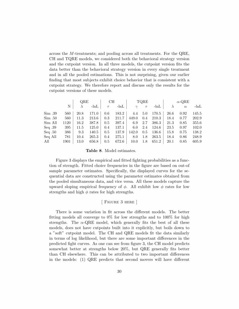
across the M -treatments; and pooling across all treatments. For the QRE,CH and TQRE models, we considered both the behavioral strategy versionand the cutpoint version. In all three models, the cutpoint version fits thedata better than the behavioral strategy version in every single treatmentand in all the pooled estimations. This is not surprising, given our earlierfinding that most subjects exhibit choice behavior that is consistent with acutpoint strategy. We therefore report and discuss only the results for thecutpoint versions of these models.

QRE CH TQRE α-QREN λ -lnL τ -lnL γ τ -lnL λ α -lnL

Sim .39 560 20.8 171.0 0.6 183.2 4.4 5.0 170.5 26.6 0.92 145.5Sim .50 560 11.3 213.6 0.3 211.7 449.0 0.4 210.3 18.4 0.77 202.9Sim All 1120 16.2 387.8 0.5 397.4 6.9 2.7 386.3 21.3 0.85 355.6Seq .39 395 11.5 125.0 0.4 137.1 6.0 2.4 124.6 23.5 0.97 102.0Seq .50 386 9.3 140.5 0.5 137.9 142.0 0.5 136.6 15.8 0.75 138.2Seq All 781 10.4 265.3 0.4 275.1 8.0 1.8 263.5 18.4 0.86 248.9All 1901 13.0 656.8 0.5 672.6 10.0 1.8 651.2 20.1 0.85 605.9

Table 8. Model estimates.

Figure 3 displays the empirical and fitted fighting probabilities as a func-tion of strength. Fitted choice frequencies in the figure are based on out-ofsample parameter estimates. Specifically, the displayed curves for the se-quential data are constructed using the parameter estimates obtained fromthe pooled simultaneous data, and vice versa. All these models capture theupward sloping empirical frequency of φ. All exhibit low φ rates for lowstrengths and high φ rates for high strengths.

[ Figure 3 here ]

There is some variation in fit across the different models. The betterfitting models all converge to 0% for low strengths and to 100% for highstrengths. The α-QRE model, which generally fits the best of all thesemodels, does not have cutpoints built into it explicitly, but boils down toa ”soft” cutpoint model. The CH and QRE models fit the data similarlyin terms of log likelihood, but there are some important differences in thepredicted fight curves. As one can see from figure 3, the CH model predictssomewhat better at strengths below 20%, but QRE generally fits betterthan CH elsewhere. This can be attributed to two important differencesin the models: (1) QRE predicts that second movers will have different

30

(and sharper) response functions than first movers, which is a feature of thedata not captured by CH; (2) QRE generates a smooth fight curve, whileCH predicts clustering of cutpoints, leading to jumps in the fight curvecorresponding to different levels of sophistication.

The TQRE model does not provide a substantial improvement over QREor CH. In fact, the fitted φ-rate for TQRE and QRE are very similar. Theyboth share the problem of overestimating the fighting rates for subjects withlow strength. The α-QRE is the best fitting of all models, as it combinesthe elements of cursedness and stochastic choice. The pure cursed equilib-rium predicts the steepest response of fighting probability as a function ofstrength. In fact, all players follow the same cutpoint strategy, which is afunction of α, the players’ degree of cursedness. Adding quantal response,produces a nice logit function of the fighting probability, that crosses .50 ats ≈ .40, varying slightly with M and position, consistent with the data. Fur-thermore, quantal response also introduces a steeper φ curve for the secondmovers than for the first movers, which is again consistent with the data.

There are some differences in fit between the M = .39 and the M = .50treatments, with most models fitting the data from the M = .39 treatmentbetter, reflecting the steeper empirical φ curves in the M = .39 data. Thereis virtually no difference in either the fit or the actual parameter estimates forthe sequential and simultaneous treatments. The α-QRE pooled estimatesof λ and α are not significantly different between the two treatments, evenat the 5% level, and the fit is identical (log Likelihood / N = −.318 in bothcases).

5.7 Summary of estimation results

The main findings about the estimated models summarized as follows.

• All four models capture the most basic qualitative properties of be-havior (none of which is consistent with Nash equilibrium): fight ratesare high, increasing in s, and decreasing in M . However, each modelcaptures different specific features of the data.

• Estimates are similar across M treatments, and little power is lostby pooling treatments. This means that the results are not due to”tuning the parameters to fit the data”. In fact, the out-of-sampleparameters from M = .39 provide virtually identical predictions forM = .50 behavior as the within sample estimates.

• Only QRE and the models hybridized with QRE capture the fact that

31

first movers behave differently from second movers. In particular, theφ function is steeper for second movers in those models.

• The cutpoint versions of CH and QRE describe behavior better thanthe behavior strategy versions. This is consistent with our findingsat the individual level which indicate that over 95% of choices followpure cutpoint strategies.

• TQRE provides an almost identical fit as QRE, suggesting that, in thisgame, the addition of hierarchical thinking to quantal response doesnot have a substantial impact. This is also consistent with the fact thatwe do not find individual cutpoints clustered around 3 or 4 strengthvalues, as would be predicted by CH and other levels-of-sophisticationmodels.

• The α-QRE model fits the data best. The estimates of α are signifi-cantly greater than 0 and significantly less than 1. They are virtuallyidentical for both the sequential and simultaneous games, suggestingthat the 2-parameter model is not overfitting the data.

6 Conclusions

The compromise game is obviously challenging to the cognitive abilities ofplayers. This is true not only for our subjects but even for experiencedmicroeconomists. In our experiment, players seem to understand some ba-sic elements of the game, such as the cutpoint nature of best responses.However, they have problems figuring out the full logic of the unravellingargument.

The paper has considered several cognitive explanations for the surpris-ing behavior observed in these games of incomplete information. In a futureresearch, it might be interesting to explore more general models. One can-didate would be the ”analogy-based expectation equilibrium” developed byJehiel and Koessler (2006), which can be seen as a generalized version ofcursed equilibrium. A second direction would be to explicitly allow for het-erogeneity. While the CH model is suggestive of heterogeneity, the attemptshere and elsewhere to fit the model assumes homogeneity, since repeatedobservations of the same individual are treated as independent draws fromthe type space. In principle, one could extend the estimation of CH modelsto allow for fixed types. However, for our data, it seems unlikely to go veryfar because we do not observe clusters of behavior that might correspond

32

to types – in contrast to Nagel’s (1995) guessing game, for example. TheQRE and α-QRE models could also be extended to allow for heterogeneitywith respect to λ and α, also with fixed types. This would undoubtedly leadto better fits in terms of log likelihood, but it is hard to imagine any newinsights emerging from such an exercise.

One of the most interesting findings is that the order of moves affectschoices. In our game, a player’s action is relevant only if the rival chooses ρ.Thus, first, second and simultaneous movers should all condition their strat-egy on that event. By contrast, the data shows that players who observeρ being played by their rival (second movers) respond more aggressivelythan players who must condition on the anticipation of that event (firstmovers). Even among subjects who do not observe the choice of the rivalbefore playing, there is a difference between knowing that one’s choices willbe publicly observed before the rival makes his choice (first movers) andknowing that one’s choices will not be observed (simultaneous movers). Insum, hypothetical conditioning on events seems to produce different behav-ior than observational conditioning on events. While we found one generalexplanation for this phenomenon (QRE), a search for other parsimoniousformal models that imply different behavior between our first and secondmovers might add to our understanding. Such a search seems a worthyproject for future research. It could also help settle questions well beyondthe scope of our compromise game, such as the effect of using the strat-egy method in experimental games, and the differences in behavior betweenstrategically equivalent games (extensive vs. strategic form). Naturally, thishas implications for many strategic settings of significant applied interest,including common value auctions and voting behavior, where optimal choicerequires bidders to condition on winning and voters to condition on beingpivotal.

33

References

[1] Akerlof, G. (1970) ”The Market for Lemons: Quality Uncertainty andthe Market Mechanism,” Quarterly Journal of Economics, 84, 488-500.

[2] Camerer, C., T. Ho, and J. Chong (2004) ”A Cognitive Hierarchy Modelof Behavior in Games,” Quarterly Journal of Economics, 119, 861-98.

[3] Camerer, C., T. Palfrey, and B. Rogers (2006) ”Heterogeneous Quan-tal Response Equilibrium and Cognitive Hierarchies,” Working Pa-per, California Institute of Technology, http://www.hss.caltech.edu/˜trp/hqre051206.pdf.

[4] Casella, A., A. Gelman, and T. Palfrey (2006) ”An Experimental Studyof Storable Votes,” Games and Economic Behavior, 57: 123-54

[5] Costa-Gomes, M. and V. Crawford (2006) ”Cognition and Behaviorin Two-Person Guessing Games: An Experimental Study,” AmericanEconomic Review, In Press.

[6] Crawford, V. and N. Iriberri (2005) ”Level-k Auctions: Can a Non-Equilibrium Model of Strategic Thinking Explain the Winner’s Curseand Overbidding in Private-Value Auctions?” Working Paper, UCSD.

[7] Eyster, E. and M. Rabin (2005) ”Cursed Equilibrium,” Econometrica,73: 1623-72.

[8] Fehr, E. and K. Schmidt (1999) ”A Theory of Fairness, Competitionand Cooperation,” Quarterly Journal of Economics, 114(3), 817-868.

[9] Forsythe, R, R.M. Isaac, and T. Palfrey (1989) ”Theories and Tests of’Blind Bidding’ in Sealed Bid Auctions,” Rand Journal of Economics,20, 214-238.

[10] Goeree, J., C. Holt, and T. Palfrey (2005), ”Regular Quantal ResponseEquilibrium,” Experimental Economics, 8, 347-367.

[11] Holt, C. and R. Sherman (1994), ”The Loser’s Curse,” American Eco-nomic Review, 84(3), 642-652.

[12] Jehiel, P. and F. Koessler (2006), ”Revisiting Games of IncompleteInformation with Analogy-Based Expectations,” Working Paper, PSE.

[13] Kagel, J and D. Levin (2002) Common Value Auctions and the Win-ner’s Curse, Princeton University Press: Princeton, NJ.

34

[14] Lynch, M., R. Miller, C. Plott, and R. Porter (1984), ”Product Qual-ity, Consumer Information, and ’Lemons’ in Experimental Markets,” inEmpirical Approaches to Consumer Protection Economics, (P. Ippolitoand D. Scheffman eds.), FTC: Washington D.C., pp. 251–306.

[15] McKelvey, R. and T. Palfrey (1995) ”Quantal Response Equilibria inNormal Form Games,” Games and Economic Behavior, 10, 6-38.

[16] McKelvey, R. and T. Palfrey (1998) ”Quantal Response Equilibria inExtensive Form Games,” Experimental Economics, 1, 9-41.

[17] Milgrom, P. and N. Stokey (1982) ”Information, Trade and CommonKnowledge,” Journal of Economic Theory, 26, 17-27.

[18] Morris, S (1994) ”Trade with Heterogeneous Prior Beliefs and Asym-metric Information,” Econometrica, 62, 1327-1347.

[19] Myerson, R.B. and M.A. Satterthwaite (1983) ”Efficient mechanismsfor bilateral trading,” Journal of Economic Theory, 29(2), 265-281.

[20] Nagel, R. (1995) ”Unraveling in Guessing Games: An ExperimentalStudy,” American Economic Review, 85(5), 1313-1326.

[21] Palfrey, T. and J. Prisbrey (1996) ”Altruism, Reputation, and Noise inLinear Public Goods Experiments,” Journal of Public Economics, 61,409-27.

[22] Samuelson, W. and M. Bazerman (1985) ”The Winner’s Curse in Bilat-eral Negotiations,” in Research in Experimental Economics (V. Smithed.), JAI press, 105-137.

[23] Sonsino, D., I. Erev, and S. Gilat (2001) ”On Rationality, Learningand Zero-Sum Betting – An Experimental Study of the No-BettingConjecture,” Working Paper, Technion.

[24] Sovic, Y. (2004) ”Strength of Dominance and Depths of Reasoning,”Working Paper, University of Oslo.

[25] Stahl, D. and P. Wilson (1995), ”On Players’ Models of Other Players:Theory and Experimental Evidence,” Games and Economic Behavior,10(July), 218-54.

[26] Wang, S. (2006), ”Misunderstanding the Other,” Mimeo, PrincetonUniversity.

35

Appendix: Sample Instruction Script

Thank you for agreeing to participate in this research experiment on group decision

making. During the experiment we require your complete, undistracted attention. So we

ask that you follow these instructions carefully. You may not open other applications on

your computer, chat with other students, or engage in other distracting activities, such as

using your cell phones or head phones, reading books, etc.

For your participation, you will be paid in cash, at the end of the experiment. Different

participants may earn different amounts. What you earn depends partly on your decisions,

partly on the decisions of others, and partly on chance. So it is important that you listen

carefully, and fully understand the instructions before we begin. You will be asked some

review questions after the instructions, which have to be answered correctly before we can

begin the paid session.

The entire experiment will take place through computer terminals, and all interaction

between you will take place through the computers. It is important that you not talk

or in any way try to communicate with other participants during the experiment except

according to the rules described in the instructions.

We will start with a brief instruction period. During the instruction period, you will

be given a complete description of the experiment and will be shown how to use the

computers. If you have any questions during the instruction period, raise your hand and

your question will be answered out loud so everyone can hear. If any difficulties arise after

the experiment has begun, raise your hand, and an experimenter will come and assist you

privately.

This experiment will begin with a brief practice session to help familiarize you with

the rules. The practice session will be followed by a paid session. You will not be paid for

the practice session.

This paid session of the experiment has 2 parts. In each part you will make choices

over a sequence of 20 different decision rounds so in total you will make 40 decisions. In

each round, you will receive a payoff, that depends on your decision that round and on

the decision of one randomly selected participant you are matched with. We will explain

exactly how these payoffs are computed in a minute.

At the end of the paid session, you will be paid the sum of what you have earned in all

40 decision rounds, plus the show-up fee of $10.00. Everyone will be paid in private and

you are under no obligation to tell others how much you earned. Your earnings during

the experiment are denominated in POINTS. Your DOLLAR earnings are determined

by multiplying your earnings in POINTS by a conversion rate. In this experiment, the

conversion rate is 0.006, meaning that 100 POINTS equals 60 cents.

Here is how each decision round, or match, works. First, the computer randomly

matches you into pairs. Since there are 14? (note to reader: depends on session) partic-

ipants in today’s session, there will be 7? (note to reader: depends on session) matched

36

pairs in each decision round. You are not told the identity of the participant you are

matched with. Your payoff depends only on your decision and the decision of the one

participant you are matched with. What happens in the other pairs has no effect on your

payoff and vice versa. Your decisions are not revealed to participants in the other pairs.

Next, the computer randomly assigns a number to you, which is equally likely to be

any number between 1 and 100. This number is called your “strength.” Each strength

number is chosen independently for each participant. Therefore usually you and the person

you are matched with will have different numbers, although there is a very small (1%)

chance the other participant in your pair has the same strength you have. You are told

your strength, but will not be told the strength of the other participant until after you

have made your decision.

You then have to make a decision to take one of two possible actions. These two

actions are called “fight” and “retreat”. If both of you choose retreat, then both of you

will receive a payoff of 40 points each. However, if either of you chooses fight, then the

one with the greater strength receives a 95 points payoff and the one with less strength

receives a 5 points payoff. Ties are broken randomly.

[SCREEN 1] This slide shows a summary of the Payoffs

Each of you must make your decision to fight or retreat at the same time, so neither

of you are told what the other participant chose (or their strength) until after both of you

have made your choices. The match is over when you and the person you are matched

with have both made a decision, and the computer will show you the results of your match

only.

When all pairs have finished the match and seen the results, we proceed to the next

match. For the next match, the computer randomly reassigns all participants to a new

pair, and randomly reassigns a new strength to each participant. Your new strength

assignment does not depend in any way on the past decisions or strengths of any partic-

ipant including yourself. Strength assignments are completely independent across pairs,

across participants, and across matches. After learning your new strength assignment,

you choose either “fight” or “retreat” and receive payoffs in a similar manner as in the

previous match.

This continues for 20 matches, at which point Part 1 of the experiment is over. I will

read you the instructions for Part 2 after we complete Part 1.

We will now begin the Practice session and go through two practice rounds. During

the practice matches, please do not hit any keys until you are asked to, and when you

enter information, please do exactly as asked. Remember, you are not paid for these 2

practice rounds. At the end of the second practice round you will have to answer some

review questions. Everyone must answer all the questions correctly before the experiment

can begin.

[AUTHENTICATE CLIENTS]

Please double click on the icon on your desktop that says “c”. When the computer

37

prompts you for your name, type your First and Last name. Then click SUBMIT and

wait for further instructions.

[START GAME]

[SCREEN 2]

You now see the first screen of the experiment on your computer. It should look

similar to this screen.

At the top left of the screen, you see your subject ID. Please record that on your

record sheet now. You have been randomly matched by the computer with exactly one of

the other participants. This pair assignment will change after each match.

You have been assigned your strength for this match, which is revealed to you on

your screen. [point on overhead]. Your exact strength number on your own screen would

probably be different from the one on this slide.

The participant you are matched with was also randomly assigned a strength, but

that will not be revealed to you until the end of the match. All you know now is that their

strength is some number between 1 and 100, with every number being equally likely.

There are two buttons, one marked “Fight” and one marked “Retreat”. You must

choose one of those two buttons, but please do not do so yet. I want to remind you how

your payoffs will be computed. If you and the person you are matched with BOTH choose

retreat, then each of you receives a 40 points payoff. If either one of you chooses fight, then

whoever has the higher strength receives 95 points and whoever has the lower strength

receives 5 points. If you have the same strength, then the computer will randomly choose

one of you to receive 95 points and the other to receive 5 points.

At this time, if your subject ID is even, please click on the button labelled “fight”. If

your subject ID is odd, please click on the button labelled “retreat”.

When everyone has made a choice, you are told the choice made by the participant you

are matched with and also told that participant’s strength. The outcome is summarized

on your screen. [show on overhead screen]

[SCREEN 3]

Each Round Summary is shown on the center of the screen.

The bottom half of your screen contains a table summarizing the results for all matches

you have participated in. This is called your history screen. It will be filled out as the

experiment proceeds. Notice that it only shows the results from your pair, not the results

from any of the other pairs. PLEASE record this information on your record sheet.

We now proceed to the next match.

For the next match you will be randomly re-matched into pairs, and randomly receive

new strength assignments.

[START next MATCH]

Please notice your new strength assignment. [Reader: Ask if everyone sees it, and

wait for confirmation from them.] Please make the opposite decision in match 2 than you

made in match 1. That is, if your subject ID is even please click on the retreat button

38

and if your subject ID is odd, please click on the “fight” button, and then wait for further

instructions.

[wait for them to complete match 2]

Practice match 2 is now over.

Please complete the review questions before we begin the paid session. Once you

answer all the questions correctly, click submit. After both participants in your pair have

answered the first round of questions, the next round of questions will appear. Please

answer all questions correctly and click submit and the quiz will disappear from your

screen. [WAIT for everyone to finish the Quiz]

Are there any questions before we begin with the paid session? We will now begin

with the 20 paid matches of Part 1. Please pull out your dividers for the paid session of

the experiment. If there are any problems or questions from this point on, raise your hand

and an experimenter will come and assist you.

[START MATCH 2]

[After MATCH 21 read:]

We have now reached the end of Part 1. Your total payoff from this part is displayed

on your screen. Please record this on your record sheet and CLICK OK. We will now give

you instructions for Part 2. Please listen carefully.

Part 2

Part 2 of the experiment will take place over a sequence of 2 practice and 20 paid

matches. This Part is almost exactly the same as Part 1, with one difference. For each

pair, one of the participants will choose to retreat or fight before the other participant

makes a choice. The other participant will then be told the first participant’s decision and

will then make their decision in response. Payoffs are computed exactly as before. For

each match, the computer randomly selects the participant to decide first, so sometimes

you will decide first and sometimes you will decide second. The assignment of who decides

first or second does not in any way depend on the strength assignment or past decisions.

The computer program just randomly assigns one participant for each pair to decide first.

We will now proceed through two practice matches to familiarize you with the screens,

which are slightly different than Part 1.

[Go to Match 22]

You now see the first screen of the experiment on your computer.

In this part of the experiment, the computer randomly assigns an order in which the

two members of your pair make decisions. If you are assigned as the first decision maker

in your match, your screen should look similar to this:

[SCREEN 4]

[Describe the screen by pointing and READ THE SCREEN]

Of course your exact strength number on your own screen would probably be different

from the one on this overhead.

39

If you are assigned as the second decision maker in your match, your screen looks like

this:

[SCREEN 5]

[Describe the screen by pointing and READ THE SCREEN]

Of course your exact strength number on your own screen would probably be different

from the one on this overhead.

The first decision maker in each pair must make a decision. If you are decision maker

one and your ID is even please click on the Fight button now. If you are decision maker

one and your ID is odd please click on the Retreat button now. If you are decision maker

two, please wait until it is your turn to make a decision.

Next, the first decision maker’s choice is revealed to the second decision maker. Please

do not make any decisions until I finish explaining. The screen looks like:

[SCREEN 6] if decision maker one chose fight, READ the SCREEN

[SCREEN 7] if decision maker one chose retreat READ the SCREEN

After viewing this information, the second decision maker is prompted to a choice.

If decision maker one chose Fight, then the outcome does not depend on decision maker

two’s choice. In this case we simply ask decision maker two to click on the “continue”

button. If decision maker one chose retreat, then the outcome does depend on decision

maker two’s choice, so decision maker two must now make a choice of fight or retreat.

This information is summarized on this slide

[SCREEN 8]

If you are decision maker two and you have a choice, if your ID is even, please click

the Retreat button now. If your ID is odd, please click on Fight now. Otherwise, please

click on the continue button now. This is important so please do not forget to do so. The

match cannot proceed until the second decision maker has clicked a button.

The results of the match are then displayed for both decision makers in the pair. The

screen should look like:

[SCREEN 9] for first decision maker

[SCREEN 10] and like this for second decision maker

We will now proceed to the second practice match [CLICK NEXT MATCH]. When

you are prompted to make a decision, please make the opposite decision from your decision

in the first practice match. That is, if your ID is even, click on Retreat, and if your ID

is odd, click on Fight. Please go ahead and make your choices. If you are decision maker

two and you see the continue button, please remember to click on it or it will delay the

experiment.

[Advance to match 23 and wait for participants to finish]

The practice match is now over. Are there any questions before we begin the 20 paid

matches?

[SCREEN 11] Here is a summary of the Payoff

[START MATCH 24]

40

[After MATCH 44, read:]

Your Total Payoff for both parts is displayed on your screen. Please record this payoff

on your record sheet and remember to CLICK OK after you are done.

[CLICK ON WRITE OUTPUT]

Your total payoff is this amount plus the show-up fee of $10. We will pay each of you

in private in the next room in the order of your Subject ID number. Remember you are

under no obligation to reveal your earnings to the other players.

Please put the mouse behind the computer and do not use either the mouse or the

keyboard at all. Please remain seated and keep the dividers pulled out until we call you

to be paid. Do not converse with the other participants or use your cell phone while in

the laboratory.

Thank you for your cooperation.

Could the person with ID number 0 go to the next room to be paid.

41

Figure 1. Empirical Fight Rates.

SIMULTANEOUS 39

0

0.2

0.4

0.6

0.8

1

0 10 20 30 40 50 60 70 80 90

Strength

Figh

t Rat

eSIMULTANEOUS 50

0

0.2

0.4

0.6

0.8

1

0 10 20 30 40 50 60 70 80 90

Strength

Figh

t Rat

e

SEQUENTIAL 39. PLAYER 1.

0

0.2

0.4

0.6

0.8

1

0 10 20 30 40 50 60 70 80 90

Strength

Figh

t Rat

e

SEQUENTIAL 50. PLAYER 1.

0

0.2

0.4

0.6

0.8

1

0 10 20 30 40 50 60 70 80 90

Strength

Figh

t Rat

e

SEQUENTIAL 39. PLAYER 2.

0

0.2

0.4

0.6

0.8

1

0 10 20 30 40 50 60 70 80 90

Strength

Figh

t Rat

e

SEQUENTIAL 50. PLAYER 2.

0

0.2

0.4

0.6

0.8

1

0 10 20 30 40 50 60 70 80 90

Strength

Figh

t Rat

e

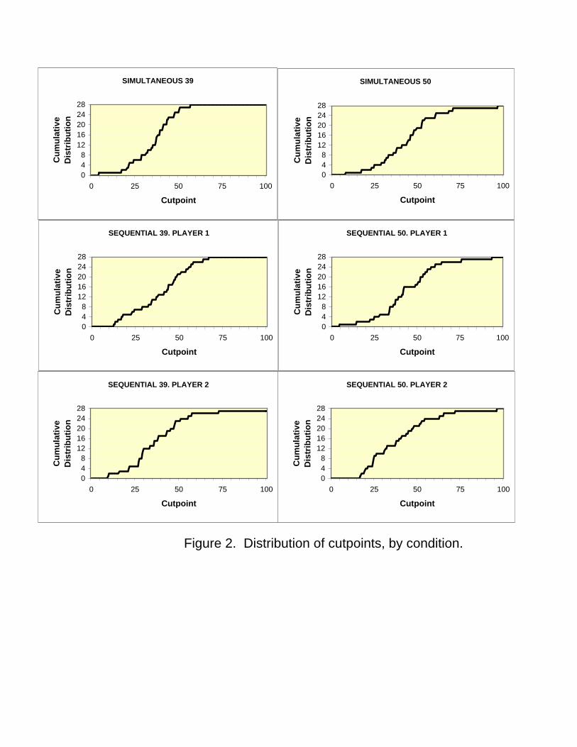
Figure 2. Distribution of cutpoints, by condition.

SEQUENTIAL 39. PLAYER 1

048

1216202428

0 25 50 75 100

Cutpoint

Cum

ulat

ive

Dis

trib

utio

nSIMULTANEOUS 50

048

1216202428

0 25 50 75 100

Cutpoint

Cum

ulat

ive

Dis

trib

utio

n

SIMULTANEOUS 39

048

1216202428

0 25 50 75 100

Cutpoint

Cum

ulat

ive

Dis

trib

utio

n

SEQUENTIAL 50. PLAYER 2

048

1216202428

0 25 50 75 100

Cutpoint

Cum

ulat

ive

Dis

trib

utio

n

SEQUENTIAL 39. PLAYER 2

048

1216202428

0 25 50 75 100

Cutpoint

Cum

ulat

ive

Dis

trib

utio

n

SEQUENTIAL 50. PLAYER 1

048

1216202428

0 25 50 75 100

Cutpoint

Cum

ulat

ive

Dis

trib

utio

n

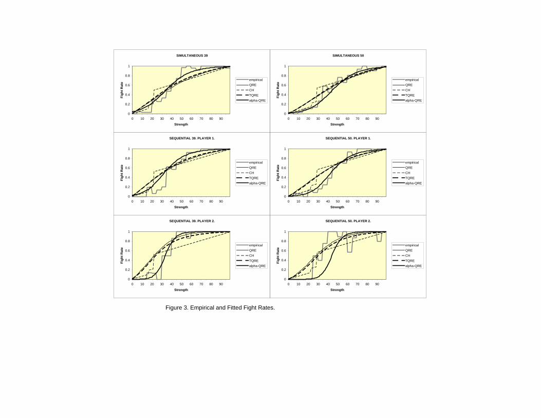
Figure 3. Empirical and Fitted Fight Rates.

SIMULTANEOUS 39

0

0.2

0.4

0.6

0.8

1

0 10 20 30 40 50 60 70 80 90

StrengthFi

ght R

ate

empiricalQRECHTQREalpha-QRE

SIMULTANEOUS 50

0

0.2

0.4

0.6

0.8

1

0 10 20 30 40 50 60 70 80 90

Strength

Figh

t Rat

e

empiricalQRECHTQREalpha-QRE

SEQUENTIAL 39. PLAYER 1.

0

0.2

0.4

0.6

0.8

1

0 10 20 30 40 50 60 70 80 90

Strength

Figh

t Rat

e

empiricalQRE

CH

TQREalpha-QRE

SEQUENTIAL 50. PLAYER 1.

0

0.2

0.4

0.6

0.8

1

0 10 20 30 40 50 60 70 80 90

Strength

Figh

t Rat

e

empiricalQRECHTQREalpha-QRE

SEQUENTIAL 39. PLAYER 2.

0

0.2

0.4

0.6

0.8

1

0 10 20 30 40 50 60 70 80 90

Strength

Figh

t Rat

e

empiricalQRE

CHTQREalpha-QRE

SEQUENTIAL 50. PLAYER 2.

0

0.2

0.4

0.6

0.8

1

0 10 20 30 40 50 60 70 80 90

Strength

Figh

t Rat

e

empiricalQRECHTQREalpha-QRE