Embed Size (px)
Citation preview
Confidential manuscript submitted to Journal of Advances in Modeling Earth Systems
The Community Earth System Model version 2 (CESM2) 1
G. Danabasoglu1, J.-F. Lamarque1, J. Bacmeister1, D. A. Bailey1, A. K. DuVivier1, J. 2
Edwards1, L. K. Emmons2, J. Fasullo1, R. Garcia2, A. Gettelman1,2, C. Hannay1, M. M. 3
Holland1, W. G. Large1, P. H. Lauritzen1, D. M. Lawrence1, J. T. M. Lenaerts3, K. 4
Lindsay1, W. H. Lipscomb1, M. J. Mills2, R. Neale1, K. W. Oleson1, B. Otto-Bliesner1, A. S. 5
Phillips1, W. Sacks1, S. Tilmes2, L. van Kampenhout4, M. Vertenstein1, A. Bertini1, J. 6
Dennis5, C. Deser1, C. Fischer1, B. Fox-Kemper6, J. E. Kay7, D. Kinnison2, P. J. Kushner8, 7
V. E. Larson9, M. C. Long1, S. Mickelson5, J. K. Moore10, E. Nienhouse5, L. Polvani11, P. J. 8
Rasch12, W. G. Strand1 9
1Climate and Global Dynamics Laboratory, National Center for Atmospheric Research, Boulder, 10
CO, USA 11
2Atmospheric Chemistry Observations and Modeling Laboratory, National Center for 12
Atmospheric Research, Boulder, CO, USA 13
3Department of Atmospheric and Oceanic Sciences, University of Colorado Boulder, Boulder, 14
CO, USA 15
4Institute for Marine and Atmospheric Research Utrecht, Utrecht University, The Netherlands 16
5Computational and Information Systems Laboratory, National Center for Atmospheric 17
Research, Boulder, CO, USA 18
6Department of Earth, Environmental, and Planetary Sciences, Brown University, Providence, 19
RI, USA 20
7Cooperative Institute for Research in Environmental Sciences, University of Colorado Boulder, 21
Boulder, CO, USA 22
8Department of Physics, University of Toronto, Toronto, ON, Canada 23
9Department of Mathematical Sciences, University of Wisconsin – Milwaukee, Milwaukee, WI, 24
USA 25
10Department of Earth System Science, University of California Irvine, Irvine, CA, USA 26
11Applied Mathematics / Earth and Environmental Sciences, Columbia University, New York, 27
NY, USA 28
12Atmospheric Science and Global Change Division, Pacific Northwest National Laboratory, 29
Richland, WA, USA 30
Corresponding author: Gokhan Danabasoglu ([email protected]) 31

Confidential manuscript submitted to Journal of Advances in Modeling Earth Systems
2
Key Points: 32
• Community Earth System Model version 2 includes many substantial science and 33
infrastructure improvements since its previous version. 34
• Preindustrial control and historical simulations were performed with low-top and high-top 35
with comprehensive chemistry atmospheric models. 36
• Comparisons to observations are improved relative to previous versions, including major 37
reductions in radiation and precipitation biases. 38
39
Keywords: Community Earth System Model (CESM); Global coupled Earth system modeling; 40
Pre-industrial and historical simulations; Coupled model development and evaluation 41
Confidential manuscript submitted to Journal of Advances in Modeling Earth Systems
3
Abstract 42
An overview of the Community Earth System Model version 2 (CESM2) is provided, including 43
a discussion of the challenges encountered during its development and how they were addressed. 44
In addition, an evaluation of a pair of CESM2 long pre-industrial control and historical ensemble 45
simulations is presented. These simulations were performed using the nominal 1° horizontal 46
resolution configuration of the coupled model with both the “low-top” (40 km, with limited 47
chemistry) and “high-top” (140 km, with comprehensive chemistry) versions of the atmospheric 48
component. CESM2 contains many substantial science and infrastructure improvements and new 49
capabilities since its previous major release, CESM1, resulting in improved historical 50
simulations in comparison to CESM1 and available observations. These include major reductions 51
in low latitude precipitation and short-wave cloud forcing biases; better representation of the 52
Madden-Julian Oscillation; better El Niño – Southern Oscillation-related teleconnections; and a 53
global land carbon accumulation trend that agrees well with observationally-based estimates. 54
Most tropospheric and surface features of the low- and high-top simulations are very similar to 55
each other, so these improvements are present in both configurations. CESM2 has an equilibrium 56
climate sensitivity of 5.1-5.3°C, larger than in CESM1, primarily due to a combination of 57
relatively small changes to cloud microphysics and boundary layer parameters. In contrast, 58
CESM2’s transient climate response of 1.9-2.0°C is comparable to that of CESM1. The model 59
outputs from these and many other simulations are available to the research community, and they 60
represent CESM2’s contributions to the Coupled Model Intercomparison Project phase 6 61
(CMIP6). 62

Confidential manuscript submitted to Journal of Advances in Modeling Earth Systems
4
Plain Language Summary 63
The Community Earth System Model (CESM) is an open-source, comprehensive model used in 64
simulations of the Earth’s past, present, and future climates. The newest version, CESM2, has 65
many new technical and scientific capabilities ranging from a more realistic representation of 66
Greenland's evolving ice sheet, to the ability to model in detail how crops interact with the larger 67
Earth system, to improved representation of clouds and rain, and to the addition of wind-driven 68
waves on the model's ocean surface. The datasets from a large set of simulations that include 69
integrations for the pre-industrial conditions (1850s) and for the 1850-2014 historical period are 70
available to the community, representing CESM2’s contributions to the Coupled Model 71
Intercomparison Project phase 6 (CMIP6). 72
1 Introduction 73
The Community Earth System Model version 2 (CESM2) is the latest generation of the coupled 74
climate / Earth system models developed as a collaborative effort between scientists, software 75
engineers, and students from the National Center for Atmospheric Research (NCAR), 76
universities, and other research institutions. The CESM2 builds on many successes of its 77
predecessors. The first global coupled climate model that did not use any flux corrections, which 78
were previously required to stabilize coupled simulations even in the absence of changed 79
radiative forcing, was developed at NCAR. Washington and Meehl [1989] performed several 80
short (multi-decadal) simulations with this model to study climate sensitivity. The first coupled 81
climate model to achieve a stable present-day control simulation without any flux corrections 82
after long multi-century integrations was the Climate System Model [CSM; Boville and Gent, 83
1998]. This latter effort was followed by the Community Climate System Model version 2 84
Confidential manuscript submitted to Journal of Advances in Modeling Earth Systems
5
[CCSM2; Kiehl and Gent, 2004], the CCSM3 [Collins et al., 2006], and the CCSM4 [Gent et al., 85
2011]. Additional capabilities such as interactive carbon – nitrogen cycling, global dynamic 86
vegetation and land use change due to anthropogenic activities, a marine biogeochemistry 87
module, a dynamic ice sheet model, and new chemical and physical processes for direct and 88
indirect aerosol effects were added to develop CCSM into an Earth system model. With these 89
new capabilities, the model was renamed the Community Earth System Model [CESM1; Hurrell 90
et al., 2013]. 91
These CCSM and CESM versions have been at the forefront of national and international efforts 92
to understand and predict the behavior of Earth's climate. Output from numerous simulations 93
using CCSM and CESM has been routinely used in studies to better understand the processes 94
and mechanisms responsible for climate variability and change. Most of these studies make use 95
of CCSM’s and CESM’s contributions to the various phases of the Coupled Model 96
Intercomparison Project (CMIP). Evaluation of those contributions has identified CCSM and 97
CESM as among the most realistic climate models in the world based on a few metrics that 98
compare the model outputs against present-day observationally-based datasets [Knutti et al., 99
2013]. In addition, CESM1 has also been used in key activities to advance our understanding of 100
the climate system and its variability and predictability, by supplementing CESM1’s 101
contributions to the CMIPs with other community-driven science efforts. These include the 102
CESM1 Large Ensemble [CESM1(LENS); Kay et al., 2015], the CESM Decadal Prediction 103
Large Ensemble [CESM-DPLE; Yeager et al., 2018], the CESM Last Millennium Ensemble 104
[CESM-LME; Otto-Bliesner et al., 2016], and the CESM Stratospheric Aerosol Geoengineering 105
Large Ensemble [GLENS; Tilmes et al., 2018]. 106
Confidential manuscript submitted to Journal of Advances in Modeling Earth Systems
6
The CESM2 was released to the community in June 2018 (available at 107
www.cesm.ucar.edu:/models/cesm2/). Simulations with the model have been done as 108
contributions to the CMIP phase 6 [CMIP6; Eyring et al., 2016] using the nominal 1° horizontal 109
resolution configuration with both the so-called “low-top” (limited chemistry) and “high-top” 110
with comprehensive chemistry versions of the atmospheric model (see Section 2). Following the 111
notation introduced in Hurrell et al. [2013], these configurations will be referred to as 112
CESM2(CAM6) and CESM2(WACCM6), respectively. CMIP6-required core simulations are 113
the so-called Diagnostic, Evaluation, and Characterization of Klima (DECK) experiments that 114
consist of a long pre-industrial (PI) control simulation; an abrupt quadrupling of CO2 115
concentration simulation; a 1% per year CO2 concentration increase simulation; and an AMIP 116
(Atmospheric Model Intercomparison Project) simulation forced with prescribed observed sea 117
surface temperatures (SSTs) and sea-ice concentrations. These are complemented by multiple 118
simulations of the historical (1850-2014) period. In addition, CESM2 is participating in about 20 119
Model Intercomparison Projects (MIPs) within CMIP6, including the ScenarioMIP which 120
requests future-projection simulations driven by alternative plausible futures of emissions and 121
land use [O’Neill et al., 2016]. The output fields from these CESM2 simulations have been 122
posted on the Earth System Grid Federation (ESGF; https://esgf-node.llnl.gov/search/cmip6). To 123
expedite the use of CESM2 by the community primarily for CMIP6-related science and 124
simulations, two incremental releases of CESM2 with the same base code as in the June 2018 125
release were made available in December 2018 (CESM2.1.0) and in June 2019 (CESM2.1.1). 126
These two releases contain additional configurations from which many of the CMIP6 127
experiments can be run as out-of-the-box simulations. 128
Confidential manuscript submitted to Journal of Advances in Modeling Earth Systems
7
This manuscript provides an overview of the CESM2 as well as an evaluation of the solutions 129
from CESM2(CAM6) and CESM2(WACCM6) PI control simulations and from the subsequent 130
ensemble sets of historical simulations with 11 and 3 members, respectively. Section 2 131
summarizes the major new features and capabilities introduced in each component model since 132
CESM1. Section 3 briefly documents challenges encountered during the development process 133
and the strategies adopted to address them. Initial conditions and forcing datasets used in the 134
simulations are detailed in Sections 4 and 5, respectively. Information on model tuning, spin-up, 135
and drifts in the PI control simulations is presented in Section 6. Highlights from primarily the 136
historical simulations that include variables from many component models are presented in 137
Sections 7-11. CESM2 results are shown with respect to CESM1 PI control and CESM1(LENS) 138
historical simulations as well as available observations. Section 12 briefly discusses the new 139
model’s equilibrium climate sensitivity and transient climate response. Finally, Section 13 140
provides a summary and discussion. While much of our analysis makes use of the full set of 141
ensemble members available, in a few instances fewer (or even one) ensemble members are used 142
for clarity and simplicity as many of the simulation characteristics or improvements are robust 143
across the ensemble members. Solutions from the PI control and historical simulations as well as 144
many other CESM2 DECK and MIP simulations are analyzed and documented in more detail in 145
the manuscripts collected as part of the AGU CESM2 Virtual Special Issue. 146
2 CESM2 and its Components 147
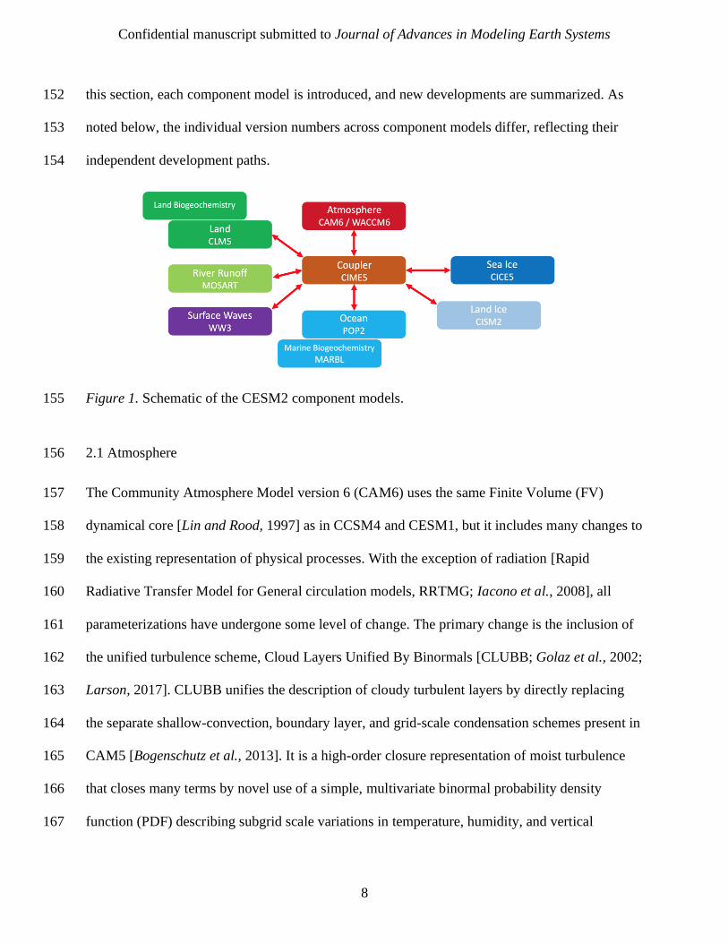
The CESM2 is an open-source community coupled model consisting of ocean, atmosphere (both 148
low-top and high-top with comprehensive chemistry), land, sea-ice, land-ice, river, and wave 149
models that exchange states and fluxes via a coupler (Fig. 1). It contains many substantial 150
science and infrastructure improvements and capabilities since its previous version, CESM1. In 151
Confidential manuscript submitted to Journal of Advances in Modeling Earth Systems
8
this section, each component model is introduced, and new developments are summarized. As 152
noted below, the individual version numbers across component models differ, reflecting their 153
independent development paths. 154
Figure 1. Schematic of the CESM2 component models. 155
2.1 Atmosphere 156
The Community Atmosphere Model version 6 (CAM6) uses the same Finite Volume (FV) 157
dynamical core [Lin and Rood, 1997] as in CCSM4 and CESM1, but it includes many changes to 158
the existing representation of physical processes. With the exception of radiation [Rapid 159
Radiative Transfer Model for General circulation models, RRTMG; Iacono et al., 2008], all 160
parameterizations have undergone some level of change. The primary change is the inclusion of 161
the unified turbulence scheme, Cloud Layers Unified By Binormals [CLUBB; Golaz et al., 2002; 162
Larson, 2017]. CLUBB unifies the description of cloudy turbulent layers by directly replacing 163
the separate shallow-convection, boundary layer, and grid-scale condensation schemes present in 164
CAM5 [Bogenschutz et al., 2013]. It is a high-order closure representation of moist turbulence 165
that closes many terms by novel use of a simple, multivariate binormal probability density 166
function (PDF) describing subgrid scale variations in temperature, humidity, and vertical 167
Confidential manuscript submitted to Journal of Advances in Modeling Earth Systems
9
velocity. The Morrison-Gettelman cloud microphysics scheme [MG1; Morrison and Gettelman, 168
2008] has been replaced by an updated version [MG2; Gettelman and Morrison, 2015], which is 169
now able to forecast, instead of diagnose, the mass and number concentration of falling 170
condensed species (rain and snow). Notably, mixed phase ice nucleation depends on aerosols, 171
rather than just temperature, following Hoose et al. [2010], as implemented in CESM2 by Wang 172
et al. [2014] with modifications of Shi et al. [2015]. Aerosols are treated using the Modal 173
Aerosol Model version 4 [MAM4; Liu et al., 2016]. A new subgrid orographic form drag 174
parameterization [Beljaars et al., 2004] replaces the Turbulent Mountain Stress (TMS) scheme, 175
and now operates with a diagnosed profile that may extend above the surface level. An 176
anisotropic orographic gravity wave drag scheme following Scinocca and McFarlane [2000] 177
represents vertically propagating gravity waves and near-surface drag as a function of mountain 178
ridge orientation and height to more accurately represent the dependence on near-surface flow 179
direction and mountain orientation. The workhorse version of CAM6 uses a nominal 1° (1.25° in 180
longitude and 0.9° in latitude) horizontal resolution with 32 vertical levels and a model top at 181
2.26 hPa (about 40 km). This version of the model has relatively coarse stratospheric 182
representation (and no prognostic chemistry module for ozone and other stratospheric 183
constituents) and is thus referred to as a “low-top” model. 184
The Whole Atmosphere Community Climate Model version 6 (WACCM6) in CESM2 is 185
configured identically to CAM6, except that it uses 70 vertical levels and its model top is at 186
4.5x10⁻⁶ hPa (about 130 km). CAM6 and WACCM6 share the same vertical level structure 187
between the surface and 87 hPa. Compared to CAM6, this version of the model has superior 188
stratospheric representation and is thus referred to as a “high-top” model. WACCM6 features a 189
comprehensive chemistry mechanism with a description of tropospheric, stratospheric, and 190
Confidential manuscript submitted to Journal of Advances in Modeling Earth Systems
10
upper-atmospheric chemistry. The default WACCM6 chemical mechanism contains 228 191
prognostic chemical species with reactions relevant for the whole atmosphere: Troposphere, 192
Stratosphere, Mesosphere, and Lower Thermosphere (TSMLT). In particular, it includes an 193
extensive representation of secondary organic aerosols [Tilmes et al., 2019]. MAM4 has been 194
modified to incorporate a new prognostic stratospheric aerosol capability [Mills et al., 2016]. The 195
modifications include mode width changes, growth of sulfate aerosol into the coarse mode, and 196
the evolution of stratospheric sulfate aerosol from natural and anthropogenic emissions of source 197
gases, including carbonyl sulfide (OCS) and volcanic sulfur dioxide (SO2). As described by 198
Gettelman et al. [2019a] and as also shown below, WACCM6 simulates nearly the same climate 199
as CAM6 in CESM2, with slight differences due to aerosol responses to chemistry, and upper 200
atmospheric processes above the CAM6 model top. WACCM6 also simulates internal variability 201
in the stratosphere, including Stratospheric Sudden Warming (SSW) events on the intraseasonal 202
timescales and the explicitly-resolved Quasi-Biennial Oscillation. 203
2.2 Ocean 204
The CESM2 ocean component is the same as in CCSM4 and CESM1, but features several 205
physics and numerical improvements; it is a level-coordinate model based on the Parallel Ocean 206
Program version 2 [POP2; Smith et al., 2010], as described in Danabasoglu et al. [2012]. The 207
physics advances include a new parameterization for mixing effects in estuaries, which improves 208
the representation of the exchange of freshwater between the terrestrial and marine branches of 209
the hydrologic cycle [Sun et al., 2019]; increased mesoscale eddy (isopycnal) diffusivities at 210
depth to improve the representation of passive tracers; use of prognostic chlorophyll for short-211
wave absorption; use of salinity-dependent freezing-point together with the sea-ice model [Assur, 212
1958]; and a new Langmuir mixing parameterization in conjunction with the new wave model 213

Confidential manuscript submitted to Journal of Advances in Modeling Earth Systems
11
component [Li et al., 2016; also see below]. The numerical improvements include a new iterative 214
solver for the barotropic mode to reduce communication costs, particularly advantageous for 215
high-resolution simulations on large processor counts [Huang et al., 2016]; a tracer-conserving 216
time filtering scheme based on an adaption of the Robert – Asselin filter to enable sub-diurnal 217
coupling of the ocean model [Robert, 1966; Asselin, 1972; Williams, 2011]; and subsequently, 218
use of a one-hour coupling frequency to explicitly resolve (sub-)diurnal and inertial periods. In 219
addition, the K-Profile vertical mixing Parameterization [KPP; Large et al., 1994] is 220
incorporated via the Community ocean Vertical Mixing (CVMix) framework, and the Caspian 221
Sea is treated as a lake in the land model and thus it is no longer included in the ocean model as a 222
marginal sea. The model uses spherical coordinates in the Southern Hemisphere. In the Northern 223
Hemisphere, the grid North Pole is displaced into Greenland. The horizontal resolution is 224
nominal 1° with a uniform resolution of 1.125° in the zonal direction. The resolution varies 225
significantly in the meridional direction with the finest resolution of 0.27° at the equator. In the 226
Southern Hemisphere, the resolution monotonically increases to 0.53° at 32°S, remaining 227
constant further south. In the Northern Hemisphere high latitudes, the finest resolution is about 228
0.38°, occurring in the northwestern Atlantic Ocean, and the coarsest resolution is about 0.64°, 229
located in the northwestern Pacific Ocean. There are 60 levels in the vertical, with a maximum 230
depth of 5500 m. The vertical resolution is uniform at 10 m in the upper 160 m and increases 231
monotonically to a maximum of 250 m by a depth of 3500 m. 232
Ocean biogeochemistry in CESM2 is represented by the Marine Biogeochemistry Library 233
(MARBL), configured to implement an updated version of what has previously been known as 234
the Biogeochemistry Elemental Cycle [BEC; Moore et al., 2002; 2004; 2013]. MARBL 235
represents multiple nutrient co-limitation (N, P, Si, and Fe), includes three explicit phytoplankton 236
Confidential manuscript submitted to Journal of Advances in Modeling Earth Systems
12
functional groups (diatoms, diazotrophs, and pico/nano phytoplankton), and one implicit group 237
(calcifiers); and there is one zooplankton group [Moore et al., 2004]. MARBL includes fully 238
prognostic carbonate chemistry and simulates sinking particulate organic matter implicitly, 239
subject to ballasting by mineral dust, biogenic CaCO3, and Si following Armstrong et al. [2002]. 240
Major updates relative to CESM1 include a representation of subgrid-scale variations in light 241
[Long et al., 2015], variable C:P stoichiometry [Galbraith and Martiny, 2015], burial of material 242
at the seafloor that matches riverine inputs in the pre-industrial climate, both semi-labile and 243
refractory dissolved organic material pools [Letscher et al., 2015], prognostic oceanic emission 244
of ammonia [Paulot et al., 2015], and an explicit ligand tracer that complexes iron. Atmospheric 245
deposition of iron is computed prognostically as a function of dust and black carbon deposition 246
simulated by CAM6. Riverine nutrient, carbon, and alkalinity fluxes are supplied to the ocean 247
from a dataset. These fluxes are held constant using data from GlobalNEWS [Mayorga et al., 248
2010] with the exception of inorganic nitrogen and phosphorus fluxes, which are taken from the 249
Integrated Model to Assess the Global Environment-Global Nutrient Model (IMAGE-GNM) 250
[Beusen et al., 2015; 2016] and vary from 1900 through 2005. Outside this period, the fluxes are 251
held constant using the closest temporal value. 252
Version 3.14 of the NOAA WaveWatch-III ocean surface wave prediction model [Tolman, 2009] 253
is incorporated in CESM2 as a new component. The wave model is solved on a coarse 254
resolution, near-global grid (78.4°S – 78.4°N) with a resolution of 4° in longitude and 3.25° in 255
latitude with 25 frequency and 24 direction bins, optimized for climate applications of the Stokes 256
drift, called the ww3a grid. The waves are driven by winds, air-sea temperature differences, 257
mixed layer depth, and ocean currents provided through the coupler, and they deliver three new 258
benefits. First, the waves provide the forcing necessary for including Langmuir, or wave-driven, 259
Confidential manuscript submitted to Journal of Advances in Modeling Earth Systems
13
turbulence in the KPP vertical mixing scheme in POP2 [Li et al., 2016]. Second, wave statistics 260
from CMIP6 experiments will be contributed to the Coordinated Ocean Wave Climate Project 261
(COWCLIP) experiment [Hemer et al., 2012], which studies changes in wave climate under 262
climate change. The CESM2 contribution is expected to be unique in COWCLIP comparison as 263
the waves will be run in a fully coupled system. Third, wave statistics are now available for 264
development of other wave-related process studies and parameterizations, such as drag and gas 265
transfer coefficients that depend on sea state [Reichl et al., 2014], waves in the marginal ice 266
zones [Roach et al., 2018], wave effects on the mean flow that become important at mesoscale-267
permitting ocean model resolutions [e.g., McWilliams and Fox-Kemper, 2013; Suzuki and Fox-268
Kemper, 2016], and other climate effects of waves [Cavaleri et al., 2012]. The CESM2 default 269
version of Langmuir mixing includes only enhanced mixing within the mixed layer [McWilliams 270
and Sullivan, 2000; Li et al., 2016], but a scheme with more accurate entrainment at the mixed 271
layer base is also available [Li et al., 2017]. When the prognostic wave model is not used, a 272
statistical theory prediction of the needed variables of the wave state based on empirical 273
relationships observed in surface waves can be used instead. This “theory wave” feature in 274
CVMix provides similar Langmuir mixing effects at a much lower cost [Li and Fox-Kemper, 275
2017; Reichl and Li, 2019], with a minimal loss of accuracy for the Langmuir mixing 276
application. 277
2.3 Sea-ice 278
CESM2 uses CICE version 5.1.2 [CICE5; Hunke et al., 2015] as its sea-ice component. 279
Compared to CESM1, the sea-ice model now incorporates mushy-layer thermodynamics [Turner 280
and Hunke, 2015], with a prognostic vertical profile of ice salinity. To accomplish this, the 281
model parameterizes the gravity drainage of brine, melt water flushing within the ice, and 282
Confidential manuscript submitted to Journal of Advances in Modeling Earth Systems
14
salinity effects of snow-ice formation. The sea-ice vertical resolution has been enhanced from 283
four layers in CESM1 to eight layers in CESM2 to better resolve the salinity and temperature 284
profiles. Also, the snow model now resolves three layers to represent the vertical temperature 285
profile. The melt pond parameterization has been updated [Hunke et al., 2013] and now accounts 286
for the fact that ponds preferentially form on undeformed sea ice. In conjunction with the ocean 287
model, a salinity-dependent freezing temperature is incorporated [Assur, 1958]. CICE5 shares 288
the same horizontal grid with the ocean component. 289
2.4 Land-ice 290
The land-ice modeling capabilities introduced in CESM1 [Hurrell et al., 2013; Lipscomb et al., 291
2013] have been extended in CESM2. CESM1 used the Glimmer Community Ice Sheet Model (a 292
serial code with simplified shallow-ice dynamics) and was limited to one-way coupling; the ice 293
sheet could respond dynamically to surface mass balance (SMB) forcing from the land model, 294
but land surface topography and surface types could not evolve. The ice sheet component of 295
CESM2 is the Community Ice Sheet Model version 2.1 [CISM2.1; Lipscomb et al., 2019], a 296
state-of-the-art parallel model with higher-order velocity solvers (valid for fast-flowing ice 297
streams and ice shelves) and improved treatments of basal sliding, iceberg calving, and other 298
physical processes. The simulations in this manuscript assume fixed ice sheets, but CESM2 also 299
supports two-way coupling between the Greenland ice sheet and the land and atmosphere 300
models. For two-way coupling, land surface types and surface elevation evolve as the ice sheet 301
advances and retreats, with total water mass conserved. The ice sheet model typically is run on 302
the Greenland domain at 4 km grid resolution with a depth-integrated higher-order solver 303
[Goldberg, 2011], a pseudo-plastic basal sliding law [Aschwanden et al., 2016], and with floating 304
ice immediately calved. CESM2 simulations with dynamic Antarctic and paleo ice sheets are not 305
Confidential manuscript submitted to Journal of Advances in Modeling Earth Systems
15
yet supported but are under development. With either fixed or dynamic ice sheets, the SMB and 306
surface temperature over ice sheets are computed in CLM5 in multiple elevation classes for each 307
glaciated grid cell [Lipscomb et al., 2013]. By default, these calculations are done for any 308
CESM2 simulation with an active land model, unlike CESM1 in which ice sheet SMB was 309
computed only in a few custom simulations [e.g., Vizcaíno et al., 2013]. For Greenland, the SMB 310
and surface temperature are passed to the coupler and downscaled to the finer CISM grid, with 311
linear interpolation between elevation classes in the vertical direction and bilinear interpolation 312
in the horizontal. For Antarctica, the SMB is computed in multiple elevation classes in CLM5 313
but is not downscaled by the coupler. 314
2.5 Land 315
The Community Land Model version 5 [CLM5; Lawrence et al., 2019] includes an extensive 316
suite of new and updated processes and parameterizations. Collectively, these developments 317
improve the model’s hydrological and ecological realism and enhance the representation of 318
anthropogenic land use activities on climate and the carbon cycle. Specifically, the main updates 319
are as follows: photosynthesis updates (canopy scaling, co-limitation [Bonan et al., 2011], and 320
temperature acclimation [Lombardozzi et al., 2015]); soil hydrology improvements (frozen soil 321
hydrology updates [Swenson et al., 2012], spatially-explicit soil depth [Brunke et al., 2016], dry 322
surface layer control on soil evaporation [Swenson and Lawrence, 2014], and updated 323
groundwater scheme [Swenson and Lawrence, 2015]); snow model updates (new snow cover 324
fraction parameterization [Swenson and Lawrence, 2012], new fresh snow density 325
parameterization based on temperature and wind resulting in more realistic denser snow packs, 326
new fresh grain size parameterization based on temperature, revised canopy snow interception, 327
canopy snow radiation, and snow unloading parameterizations, and 10 m snow water equivalent 328
Confidential manuscript submitted to Journal of Advances in Modeling Earth Systems
16
maximum snow pack allowing for firn formation [van Kampenhout et al., 2017]); introduction of 329
a mechanistic plant hydraulics and hydraulic redistribution scheme which explicitly models 330
water transport through roots, stems, and leaves according to a simple hydraulic framework and 331
which replaces the empirical soil moisture stress function [Kennedy et al., 2019]; a completely 332
updated lake model [Subin et al., 2012]; vertically-resolved soil biogeochemistry scheme that 333
allows for simulation of permafrost carbon [Koven et al., 2013]; addition of a global crop model 334
that represents planting, harvest, grain fill and grain yields for six crop types and includes time-335
evolving, spatially-explicit fertilization rates and irrigated areas [Levis et al., 2018]; inclusion of 336
a new fire model that has representation of natural and anthropogenic fire triggers and 337
suppression as well as agricultural, deforestation, and peat fires [Li et al., 2013; Li and 338
Lawrence, 2017]; multiple urban classes and updated urban energy model [Oleson and Feddema, 339
2019]; and improved representation of plant N dynamics to address known deficiencies in 340
CLM4. This latter improvement is accomplished by: 1) introducing flexible plant carbon : 341
nitrogen (C:N) stoichiometry [Ghimire et al., 2016], which circumvents the problematic CLM4 342
separation of potential and actual productivity fluxes that effectively decoupled leaf-level C 343
exchange from associated water and energy fluxes; 2) explicitly simulating how photosynthetic 344
capacity responds to environmental conditions through the Leaf Utilization of Nitrogen for 345
Assimilation (LUNA) module [Ali et al., 2016]; and 3) accounting for how changes in N 346
availability have consequences for plant productivity through the Fixation and Uptake of 347
Nitrogen (FUN) module, which calculates the carbon costs of N acquisition and allocates C 348
expenditure on N uptake among biological fixation, active uptake, and retranslocation [Shi et al., 349
2016]. CLM5 receives instantaneous N fluxes directly through the coupler from WACCM6 350
when it is used. Otherwise, CLM5 uses monthly N-deposition derived from prior 351
Confidential manuscript submitted to Journal of Advances in Modeling Earth Systems
17
CESM2(WACCM6) simulations. Also, irrigation is applied either with water taken from rivers, 352
if available, or diffusely from the ocean if there is not enough river water. Detailed description, 353
assessment, and characterization of CLM5 performance compared to prior CLM versions in 354
land-only configurations are provided in Lawrence et al. [2019], Wieder et al. [2019], Fisher et 355
al. [2019], and Bonan et al. [2019]. 356
2.6 River transport 357
The River Transport Model (RTM) used in CESM1 has been replaced with the Model for Scale 358
Adaptive River Transport [MOSART; Li et al., 2013]. In standard CESM2 configurations, the 359
MOSART grid resolution is 0.5° x 0.5°. In each MOSART grid cell, surface runoff received 360
from CLM5 is routed across hillslopes and then discharged along with subsurface runoff, also 361
received from CLM5, into a tributary subnetwork. This tributary subnetwork then feeds into the 362
main river channel of that grid cell that links river water from upstream grid cells to downstream 363
grid cells. A primary difference between RTM and MOSART is how river flow is calculated. 364
RTM uses a simple linear reservoir method wherein the flux of water transferred from an RTM 365
grid cell to its downstream neighbor is dependent only on the river water storage in that grid cell, 366
the mean distance between grid cells, and a globally constant effective water velocity. In 367
MOSART, river flow rates are calculated explicitly via the physically-based kinematic wave 368
method, a commonly used method in hydrology that is based on mass and momentum equations. 369
As a consequence, whereas RTM only simulates streamflow (m3 s-1), MOSART additionally 370
simulates time-varying main channel flow velocity (m s-1) and water depth, as well as subgrid 371
surface water flow in hillslopes and tributaries. MOSART requires detailed information on river 372
hydrography (i.e., parameters describing river and tributary width, depth, average slope, 373
Confidential manuscript submitted to Journal of Advances in Modeling Earth Systems
18
roughness coefficient, and dominant river length) which is derived from the global 1 km 374
HydroSheds dataset [Lehner et al., 2008]. 375
2.7 Coupling 376
CESM2 is accompanied by a new collaborative software infrastructure for building and running 377
the model system as well as for controlling state and flux exchanges among the components. 378
This framework is known as the Common Infrastructure for Modeling the Earth (CIME; 379
http://github.com/ESMCI/cime). CIME contains a significantly re-written coupling infrastructure 380
that includes modularity, multi-instance capabilities for data assimilation, and new support for 381
land-ice coupling. It also includes re-written data components that have new Python capabilities 382
and are more easily extensible. As in CESM1, the data components can replace prognostic 383
components, thereby enabling component feedbacks to be easily controlled. Examples of such 384
configurations include ocean – sea-ice coupled integrations in which the atmospheric datasets are 385
provided by a data atmosphere model, and a land-only setup where the land model is the only 386
prognostic component. CIME also provides a new Case Control System (CCS) for configuring, 387
compiling, and executing complex Earth system model experiments. CCS is an object-oriented 388
set of Python utilities that provide many new capabilities for easier portability, case generation, 389
and user customization. It records details of the model version used as well as user customization 390
of the experimental setup. Additionally, CCS has system and unit testing functionality that leads 391
to a more robust and flexible code base. CIME can be ported and tested in a stand-alone mode, 392
without any of the CESM prognostic components, as a first step in porting CESM to other 393
machines. Finally, CIME contains additional tools, such as a new statistical consistency test, that 394
allow users to quickly verify if their port of CESM2 is successful. 395
Confidential manuscript submitted to Journal of Advances in Modeling Earth Systems
19
The atmosphere, land, wave, and sea-ice components communicate state information and fluxes 396
through the coupler every atmospheric time step of 30 minutes. The only fluxes calculated in the 397
coupler are those between the atmosphere and ocean, and the coupler communicates them to the 398
ocean component every hour and to the atmosphere every 30 minutes. The land-ice component 399
communicates with the coupler once a day. The nominal 1° horizontal version of the 400
CESM2(CAM6) has a throughput of about 30 simulated years per day on 4320 processors on the 401
Cheyenne Supercomputer, corresponding to about 3450 cpu hours per simulation year. The 402
CESM2(WACCM6) version has a throughput of about 4 simulated years per day on 3780 403
processors on the same machine, corresponding to about 22700 cpu hours per simulation year, 404
roughly 7 times more expensive than CESM2(CAM6). In both CESM2(CAM6) and 405
CESM2(WACCM6) configurations, the atmosphere is scaled to near the maximum allowed by 406
the FV dycore: 1152 tasks by 3 threads. Although CAM6 and WACCM6 can run on more 407
processors, it is not cost effective to do so. Thus, the lower processor count in 408
CESM2(WACCM6) simulations is due to the ocean component which uses 256 tasks by 3 409
threads in CESM2(CAM6), but only 24 tasks by 3 threads in CESM2(WACCM6). This is 410
because the atmospheric model is much slower with WACCM6, so fewer processors are needed 411
for the ocean to keep pace. 412
3 Development Strategy and Challenges 413
Evaluations of the component model developments summarized above were done first by the 414
respective developers using both component-only and fully-coupled configurations with various 415
CCSM4 and CESM1 versions. This is in contrast to the process used during the CCSM4 416
development where initial assessments were done primarily in component-only simulations. 417
Preliminary versions of the component models were then brought together to start the first 418
Confidential manuscript submitted to Journal of Advances in Modeling Earth Systems
20
CESM2 coupled simulations in October 2015. During this development and evaluation process 419
particular attention was paid to conservation of heat and freshwater across the component 420
models, climate drifts, reasonableness of mean climate and of variability in various fields such 421
as El Niño – Southern Oscillation (ENSO) and Atlantic meridional overturning circulation 422
(AMOC) as well as making sure that the model simulations were able to reproduce observed key 423
features of the 20th century climate such as evolution of global-mean surface temperatures, 424
present-day SSTs and sea-ice distributions and trends. Unfortunately, the path to a fully-coupled 425
CESM2 version that produced acceptable simulations for CMIP6 turned out to be much longer 426
than anticipated and very challenging. Along the way, errors and bugs were discovered and 427
addressed. Progress was particularly delayed due to two major unacceptable features that were 428
not obviously related to bugs or implementation errors. The first concerned the formation of 429
unrealistically extensive sea-ice cover over the Labrador Sea region in PI control simulations. 430
The second was that the global-mean surface temperature time series in historical simulations 431
showed a significant and quite unrealistic cooling particularly during the second half of the 20th 432
century, with end-of-the-century temperatures being actually colder than in the 1850s. 433
Substantial human and computational resources were dedicated to address these major 434
challenges, as well as less serious issues, as described below. After executing over 300 435
simulations, the vast majority being fully-coupled, ranging in duration from several decades to 436
centennial, a near-final CESM2 version was created in April 2018. 437
The formation of unrealistically extensive sea-ice cover over the Labrador Sea region, extending 438
into the northern North Atlantic, in PI control simulations proved to be very challenging to 439
address robustly. In fact, this feature – not supported by available observations – emerged twice 440
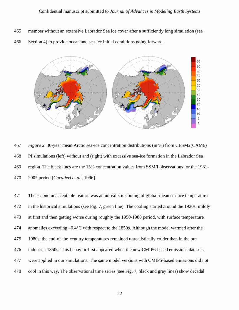
during the development process. Figure 2 shows 30-year average sea-ice concentration 441

Confidential manuscript submitted to Journal of Advances in Modeling Earth Systems
21
distributions from two CESM2(CAM6) PI simulations with and without such an extensive 442
Labrador Sea ice cover. The more extensive Labrador Sea ice extent is also accompanied by 443
enhanced (and more unrealistic) sea-ice in the Sea of Okhotsk region. In simulations with 444
extensive ice cover, this feature emerges as early as around year 40 and as late as around year 445
105 relative to initialization of the coupled simulation. In no simulation did the Labrador Sea ice 446
cover become unrealistically extensive after year 105 if it had not already emerged earlier in the 447
simulation, indicating that the model likely has multiple equilibria and the trajectory through 448
phase-space following initialization passes near a bifurcation point. It was found that extensive 449
ice cover persisted when the simulations were extended by fifty or more years further. It was not 450
feasible, given time constraints, to undertake longer integrations to investigate long-term 451
behavior of this feature. Simulation characteristics when extensive ice cover is present include: 452
annual-mean sea-ice concentrations that are usually around 60% in the Labrador Sea; Labrador 453
Sea SSTs that remain around freezing point with salinities < 34 psu; curtailed Labrador Sea deep 454
water formation / convection; compensating enhanced deep-water formation to the east of 455
Greenland and in the Irminger Sea; and a slightly weaker AMOC maintained by the switch in the 456
location of deep-water formation. Detailed analyses of many simulations with extensive ice 457
cover in comparison to simulations without this feature, unfortunately, did not identify any 458
robust mechanisms involving a particular process or phenomenon such as surface fluxes, liquid 459
and solid runoff, lateral advection, vertical mixing, and ice drag as instigators or drivers. Indeed, 460
when ensemble simulations were performed using the same model configuration but with only 461
differences in their initial atmospheric potential temperatures introduced by round-off level 462
perturbations, some members showed extensive ice cover and others did not. Given this 463
experience, a practical – though not fully satisfactory – approach was adopted to use an ensemble 464
Confidential manuscript submitted to Journal of Advances in Modeling Earth Systems
22
member without an extensive Labrador Sea ice cover after a sufficiently long simulation (see 465
Section 4) to provide ocean and sea-ice initial conditions going forward. 466
Figure 2. 30-year mean Arctic sea-ice concentration distributions (in %) from CESM2(CAM6) 467
PI simulations (left) without and (right) with excessive sea-ice formation in the Labrador Sea 468
region. The black lines are the 15% concentration values from SSM/I observations for the 1981-469
2005 period [Cavalieri et al., 1996]. 470
The second unacceptable feature was an unrealistic cooling of global-mean surface temperatures 471
in the historical simulations (see Fig. 7, green line). The cooling started around the 1920s, mildly 472
at first and then getting worse during roughly the 1950-1980 period, with surface temperature 473
anomalies exceeding –0.4°C with respect to the 1850s. Although the model warmed after the 474
1980s, the end-of-the-century temperatures remained unrealistically colder than in the pre-475
industrial 1850s. This behavior first appeared when the new CMIP6-based emissions datasets 476
were applied in our simulations. The same model versions with CMIP5-based emissions did not 477
cool in this way. The observational time series (see Fig. 7, black and gray lines) show decadal 478

Confidential manuscript submitted to Journal of Advances in Modeling Earth Systems
23
fluctuations that have significant contributions from internal variability. The cooling described 479
above clearly exceeds this baseline internal variability range and this is what is addressed here. 480
The goal is not to reproduce exactly the 20th century global-mean surface temperature time series 481
in each realization, but to eliminate the unrealistic cooling behavior. Initial investigations 482
uncovered some inconsistencies and errors in the CMIP6 emissions datasets (which were 483
resolved in their final release) and their application to CAM6, particularly for anthropogenic 484
sulfur. Simulations with the corrected datasets did show some reductions of the unrealistic 485
cooling, but the cooling behavior remained, particularly during the mid-1940s-1980 period, with 486
end-of-the-century temperatures only slightly warmer than in the 1850s (not shown). Analysis of 487
CAM6 against recent volcanic sulfur emission events indicated a potentially excessive response 488
[Malavelle et al., 2017], which could be traced to the impact of aerosols on the liquid water path. 489
Several modifications were, therefore, made to aerosol – cloud interaction processes, focusing on 490
the warm rain formation process (autoconversion and accretion) to reduce the magnitude of these 491
effects. As a result of these modifications, the global historical (2000 minus 1850) aerosol 492
effective radiative forcing changed from –1.82 W m-2 in CAM5 with CMIP5-based emissions to 493
–1.67 W m-2 in CAM6 with CMIP6-based emissions (see Gettelman et al. [2019b] for further 494
details). These changes were instrumental in enabling the model to simulate a realistic 20th 495
century surface temperature time series as discussed below (see Section 7), but they did not 496
target a particular equilibrium climate sensitivity value (see Section 12). 497
4 Initial Conditions 498
The ocean and sea-ice initial conditions used in both CESM2(CAM6) and CESM2(WACCM6) 499
PI control simulations were obtained through the following series of integrations (Fig. 3). First, a 500
3-member ensemble set of simulations was started from the CESM1(LENS) PI control 501
Confidential manuscript submitted to Journal of Advances in Modeling Earth Systems
24
integration [Kay et al., 2015] at year 402 (all simulations start from 01 January of a given year), 502
which itself was initialized from the January-mean potential temperature and salinity from the 503
Polar Science Center Hydrographic Climatology [PHC2; Steele et al., 2001; Levitus et al., 1998]. 504
Two ensemble members developed excessive Labrador Sea ice cover, starting at about year 80. 505
The third member (simulation 262c) did not show such a behavior. Therefore, it was decided to 506
use this simulation to provide ocean and sea-ice states for initializing subsequent simulations. 507
Indeed, the simulation was later extended to > 350 years to confirm that the Labrador Sea ice 508
cover remained realistic. A series of simulations with minor adjustments and bug fixes in the 509
coupled model were then performed, starting with a simulation (293) from year 161 of 510
simulation 262c. This simulation was followed by another (simulation 297) that started from year 511
130 of simulation 293. Finally, a third simulation (299) was initialized from year 249 of 512
simulation 297. The ocean and sea-ice states from year 134 of the final simulation (299) were 513
used as the initial conditions for the main CESM2(CAM6) and CESM2(WACCM6) PI control 514
simulations. Thus, in total, these ocean potential temperature and salinity initial conditions 515
Confidential manuscript submitted to Journal of Advances in Modeling Earth Systems
25
represent states integrated for about 1070 years after initialization starting from the PHC2 516
datasets. 517
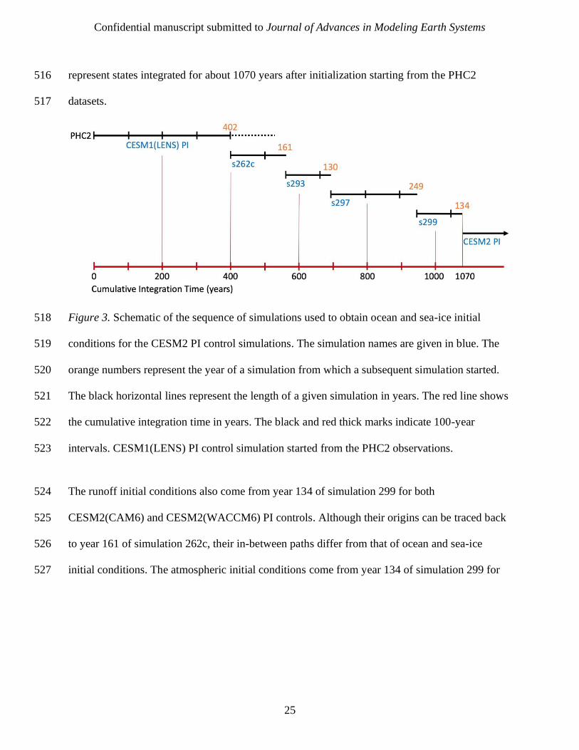
Figure 3. Schematic of the sequence of simulations used to obtain ocean and sea-ice initial 518
conditions for the CESM2 PI control simulations. The simulation names are given in blue. The 519
orange numbers represent the year of a simulation from which a subsequent simulation started. 520
The black horizontal lines represent the length of a given simulation in years. The red line shows 521
the cumulative integration time in years. The black and red thick marks indicate 100-year 522
intervals. CESM1(LENS) PI control simulation started from the PHC2 observations. 523
The runoff initial conditions also come from year 134 of simulation 299 for both 524
CESM2(CAM6) and CESM2(WACCM6) PI controls. Although their origins can be traced back 525
to year 161 of simulation 262c, their in-between paths differ from that of ocean and sea-ice 526
initial conditions. The atmospheric initial conditions come from year 134 of simulation 299 for 527
Confidential manuscript submitted to Journal of Advances in Modeling Earth Systems
26
CESM2(CAM6) PI control and year 11 of a preliminary CESM2(WACCM6) PI simulation 528
(simulation 298) for the main CESM2(WACCM6) PI control. 529
Initial conditions for the land states and ocean biogeochemical tracers, including abiotic 530
radiocarbon, were obtained with long spin-up runs of the land and ocean models, respectively. In 531
these spin-up runs, the active atmospheric component was replaced with a data-atmosphere 532
component that simply read in and repeatedly cycled through multiple years of surface forcing 533
datasets that were needed to construct surface fluxes. Twenty-one years of forcing datasets 534
extracted from simulation 297 were used, in order to capture some aspects of interannual 535
variability. The land model was spunup from bare ground, utilizing the accelerated 536
decomposition mode to equilibrate the slow carbon pools, followed by several hundred years of 537
normal mode spin-up [Lawrence et al., 2019]. The ocean tracer spin-up was applied only to the 538
biogeochemical tracers of the ocean model. To avoid drift of the ocean physical state, it was reset 539
to its initial condition at the beginning of each 21-year cycle, keeping it synchronized with the 540
surface forcing. A subset of the ocean biogeochemical tracers was spun up using a Newton-541
Krylov based solver [Lindsay, 2017]. 542
The initial conditions for the 11 members of the CESM2(CAM6) historical simulations come 543
from years 501, 601, 631, 661, 691, 721, 751, 781, 811, 841, and 871 of the corresponding PI 544
control simulation (Fig. 4). The 3 members of the CESM2(WACCM6) historical simulations are 545
initialized from years 56, 61, and 71 of the corresponding PI control integration. The late and 546
early starts dates for the CESM2(CAM6) and CESM2(WACCM6) historical simulations simply 547
reflect their respective PI control integration lengths and are not intended to avoid or sample any 548
particular variability characteristics. 549
Confidential manuscript submitted to Journal of Advances in Modeling Earth Systems
27
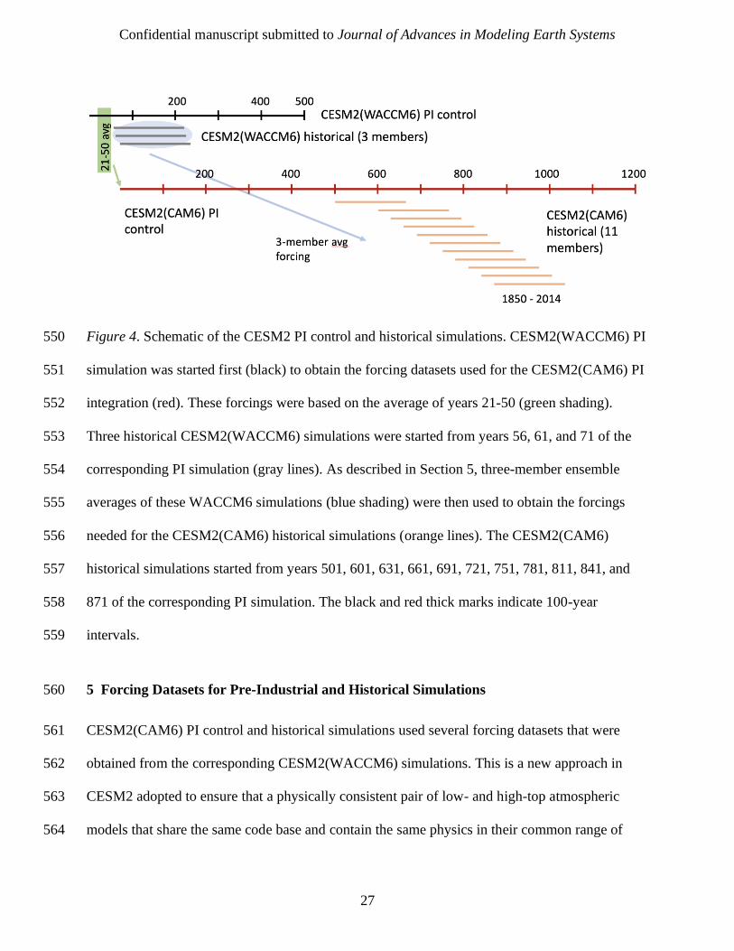
Figure 4. Schematic of the CESM2 PI control and historical simulations. CESM2(WACCM6) PI 550
simulation was started first (black) to obtain the forcing datasets used for the CESM2(CAM6) PI 551
integration (red). These forcings were based on the average of years 21-50 (green shading). 552
Three historical CESM2(WACCM6) simulations were started from years 56, 61, and 71 of the 553
corresponding PI simulation (gray lines). As described in Section 5, three-member ensemble 554
averages of these WACCM6 simulations (blue shading) were then used to obtain the forcings 555
needed for the CESM2(CAM6) historical simulations (orange lines). The CESM2(CAM6) 556
historical simulations started from years 501, 601, 631, 661, 691, 721, 751, 781, 811, 841, and 557
871 of the corresponding PI simulation. The black and red thick marks indicate 100-year 558
intervals. 559
5 Forcing Datasets for Pre-Industrial and Historical Simulations 560
CESM2(CAM6) PI control and historical simulations used several forcing datasets that were 561
obtained from the corresponding CESM2(WACCM6) simulations. This is a new approach in 562
CESM2 adopted to ensure that a physically consistent pair of low- and high-top atmospheric 563
models that share the same code base and contain the same physics in their common range of 564
Confidential manuscript submitted to Journal of Advances in Modeling Earth Systems
28
altitude is used. It represents a degree of compatibility and consistency not available to most 565
modeling groups. CESM2(WACCM6) uses CMIP6-provided forcings wherever appropriate, but 566
calculates itself chemical and aerosol constituents from emissions that are based on the 567
anthropogenic and biomass burning inventories specified by CMIP6. Anthropogenic emissions 568
for 1850 to 2014 are provided from the Community Emissions Data System [CEDS; Hoesly et 569
al., 2018]. Biomass burning emissions are described by van Marle et al. [2017] and are all 570
specified at the surface (without any plume-rise or specified vertical distribution of the 571
emissions). Further details of the emissions and chemistry used in CESM2(WACCM6), 572
including the specification of ozone-depleting substances, are described in Gettelman et al. 573
[2019a]. CESM2(CAM6) simulations use the CMIP6-provided forcings except for i) 574
tropospheric oxidants for chemistry; ii) stratospheric ozone for radiative effects; iii) stratospheric 575
aerosols for radiative effects; iv) H2O production rates due to CH4 oxidation in the stratosphere; 576
and v) N deposition to the land and ocean components. These WACCM6-based forcings are 577
described below. 578
First, CESM2(CAM6) PI simulation 299 was run with prescribed forcings from a 579
CESM2(WACCM6) simulation (295). Then the CESM2(WACCM6) PI control was conducted, 580
using initial states for the ocean, sea-ice, and land components from simulation 299 (see Section 581
4). Distributions of tropospheric oxidants, stratospheric ozone, stratospheric aerosol, and 582
methane oxidation rates were derived from the average of years 21-50 of this 583
CESM2(WACCM6) PI simulation, and used in the subsequent CESM2(CAM6) PI control. For 584
historical simulations, an ensemble of three CESM2(WACCM6) simulations was run first for the 585
1850-2015 period. Corresponding forcings were derived from the CESM2(WACCM6) ensemble 586
average, for use in the CESM2(CAM6) historical simulations. The averaging of 30 years in the 587

Confidential manuscript submitted to Journal of Advances in Modeling Earth Systems
29
PI control and of three ensemble members in the historical simulations is intended to reduce the 588
influence of natural variability on these forcings. A schematic summary of our integration 589
strategy to obtain the necessary forcing datasets to perform the CESM2(CAM6) simulations is 590
provided in Fig. 4. 591
The tropospheric oxidant species (O3, OH, NO3, and HO2) are prescribed in CESM2(CAM6), 592
which uses them in gas-phase and aerosol chemistry calculations to allow tropospheric aerosol 593
formation. Monthly-averaged values are used in both the PI control and historical simulations. 594
For the CESM2(CAM6) PI control, a repeating 12-month annual cycle is derived from averaged 595
values over years 21-50 of the CESM2(WACCM6) PI control simulation. CESM2(CAM6) 596
interpolates cyclically between mid-month date values. For CESM2(CAM6) historical 597
simulations, 12-month annual cycles are provided at quasi-decadal frequency (see Appendix A). 598
CESM2(CAM6) interpolates annual cycles for years between those provided. 599
Stratospheric ozone and stratospheric aerosol are radiatively active species important to the 600
radiative budget, temperature, general circulation, chemistry, and cloud physics of CESM2. In 601
CESM2(CAM6), stratospheric distributions of these species are prescribed from 5-day zonal 602
means of CESM2(WACCM6) output. Ozone volume mixing ratio is prescribed for the entire 603
vertical extent of the model for use in radiative transfer calculations. 604
A major advance in CESM2(WACCM6) is the development of prognostic stratospheric aerosols 605
derived from gas-phase sulfur emissions. As described in Mills et al. [2016], this new feature 606
provides CESM2 with stratospheric aerosol forcing that is much more consistent with 607
observations than previous climatologies developed for climate models. This self-consistent 608
treatment of volcanic aerosols and chemistry has been shown to produce realistic radiative 609
Confidential manuscript submitted to Journal of Advances in Modeling Earth Systems
30
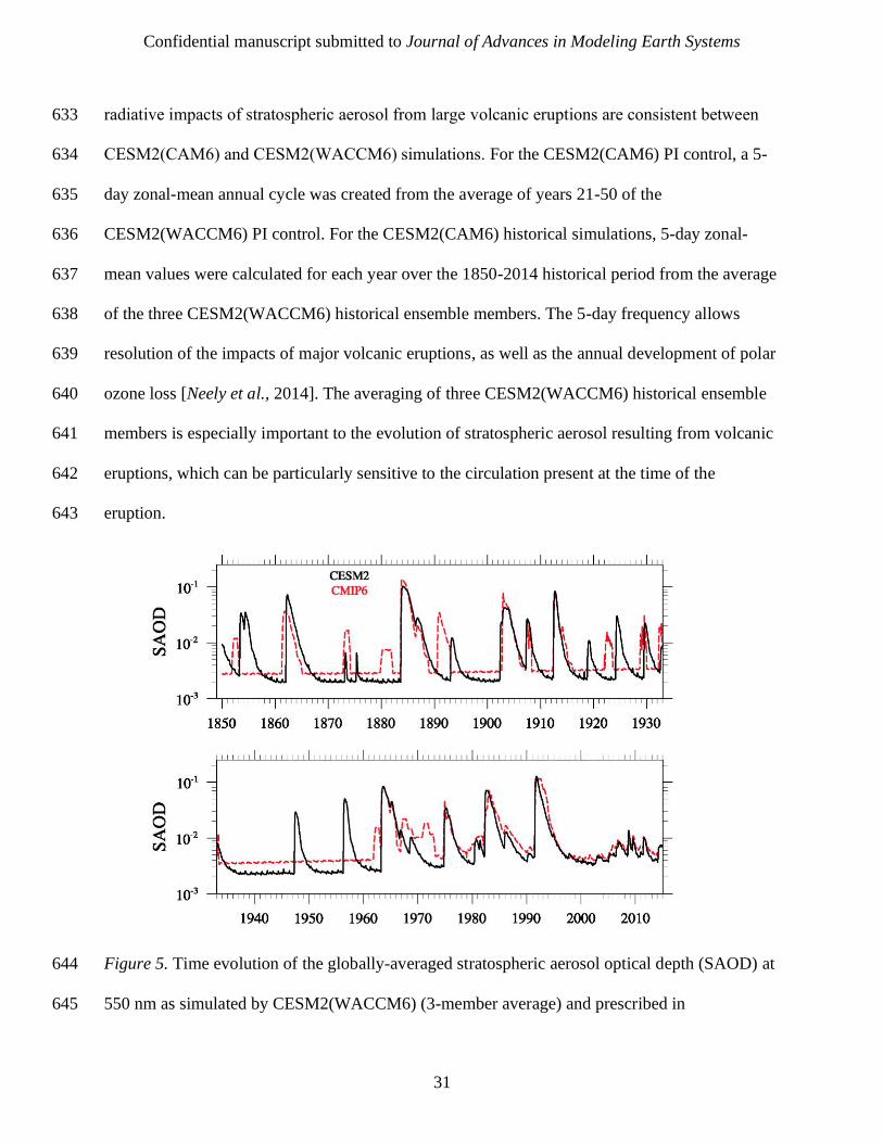
responses to eruptions over the 1979-2015 period [Mills et al., 2017; Schmidt et al., 2018]. For 610
CMIP6, volcanic SO2 emissions for 1850-2015 from VolcanEESM database [Neely and Schmidt, 611
2016] are used. In addition, observed carbonyl sulfide concentrations are specified as time-612
varying boundary conditions. As shown in Fig. 5, this leads to a realistic simulation of the 613
stratospheric aerosol optical depth (SAOD) compared to the CMIP6 data which are constrained 614
by satellite observations starting in 1979. Before this date, when the information on volcanic 615
emissions is sparser, CESM2(WACCM6) and CMIP6 SAOD can differ; for example, the 616
eruptions of Hekla (1947) and Bezymianny (1956) are missing from the CMIP6 database. Prior 617
to the satellite era, there is also a very small (~0.001) difference between CESM2(WACCM6) 618
and CMIP6 data in the background component of SAOD at 550 nm that persists during 619
volcanically quiescent periods. Historical variability in this background is largely due to 620
variability in the source gas OCS, which WACCM6 accounts for as a time-varying lower 621
boundary condition for OCS [Montzka et al., 2004]. CMIP6 prescribes a time-varying 622
background based on the 1999-2005 average, scaled following the calculations of Sheng et al. 623
[2015]. 624
Although CESM2(CAM6) does not include the interactive chemistry needed to realistically 625
simulate the development of stratospheric aerosol following a major volcanic eruption, model 626
consistency is maintained by prescribing aerosol properties above the tropopause in 627
CESM2(CAM6) using 5-day zonally averaged output from CESM2(WACCM6). Prescribed 628
stratospheric aerosol properties are the sulfate mass mixing ratio and diameter of each of the 629
three sulfate-bearing modes of MAM4, aerosol surface area density, and ice condensation nuclei 630
number concentration. Each of these properties is prescribed consistently with its use in 631
CESM2(WACCM6), which includes prognostic stratospheric aerosol in MAM4. As a result, the 632
Confidential manuscript submitted to Journal of Advances in Modeling Earth Systems
31
radiative impacts of stratospheric aerosol from large volcanic eruptions are consistent between 633
CESM2(CAM6) and CESM2(WACCM6) simulations. For the CESM2(CAM6) PI control, a 5-634
day zonal-mean annual cycle was created from the average of years 21-50 of the 635
CESM2(WACCM6) PI control. For the CESM2(CAM6) historical simulations, 5-day zonal-636
mean values were calculated for each year over the 1850-2014 historical period from the average 637
of the three CESM2(WACCM6) historical ensemble members. The 5-day frequency allows 638
resolution of the impacts of major volcanic eruptions, as well as the annual development of polar 639
ozone loss [Neely et al., 2014]. The averaging of three CESM2(WACCM6) historical ensemble 640
members is especially important to the evolution of stratospheric aerosol resulting from volcanic 641
eruptions, which can be particularly sensitive to the circulation present at the time of the 642
eruption. 643
Figure 5. Time evolution of the globally-averaged stratospheric aerosol optical depth (SAOD) at 644
550 nm as simulated by CESM2(WACCM6) (3-member average) and prescribed in 645
Confidential manuscript submitted to Journal of Advances in Modeling Earth Systems
32
CESM2(CAM6) (black) in comparison to that provided by CMIP6 (red). There is uncertainty in 646
the time, location, and intensity of volcanic emissions, especially further back in time. 647
The oxidation of methane (CH4) is an important source of water vapor to the middle atmosphere. 648
Because water vapor is a greenhouse gas, production rates of water vapor in CESM2(CAM6) are 649
prescribed using methane oxidation rates from CESM2(WACCM6). It is assumed that the 650
oxidation of each CH4 molecule results in the production of two molecules of H2O [Nicolet, 651
1970]. For the CESM2(CAM6) PI control, a repeating 12-month annual cycle is derived from 652
averaged values over years 21-50 of the CESM2(WACCM6) PI control simulation. For 653
CESM2(CAM6) historical simulations, 12-month annual cycles are provided at the same quasi-654
decadal frequency as the tropospheric oxidants (see above and Appendix A). 655
Regarding Chlorofluorocarbons (CFCs), in CESM2(CAM6), they are specified as a global 656
average mixing ratio derived from the lower boundary conditions provided by CMIP6. The 657
radiative transfer module in both CESM2(CAM6) and CESM2(WACCM6) considers only CFC-658
12 and CFC-11eq (equivalent). The CFC-11eq time series is supplied by CMIP6 [Meinshausen 659
et al., 2017]. Because CESM2(WACCM6) includes most of the chemical species contained in 660
CFC-11eq, the global distribution of CFC-11eq is first derived interactively in WACCM6. The 661
derived global average distribution at the surface is then scaled to match a given CMIP6 scenario 662
that contains additional species not included in the WACCM6 chemistry, i.e., CFC-11eq = CFC-663
11eq [CMIP6] / CFC-11eq [WACCM6]). 664
Updated land cover and land use data have been created for CLM5. The new dataset combines 665
updated versions of present-day satellite land cover descriptions with the past and future 666
transient land use time series from the Land Use Harmonization version 2 product (LUH2, 667
Confidential manuscript submitted to Journal of Advances in Modeling Earth Systems
33
http://luh.umd.edu/). CLM5 (and ocean biogeochemistry) uses monthly N-deposition derived 668
from CESM2(WACCM6) simulations. Additional information on this dataset is provided in 669
Lawrence et al. [2019] and references therein. 670
6 Pre-Industrial Control Spin-up and Tuning 671
The CESM2(CAM6) and CESM2(WACCM6) PI control simulations were integrated for 1200 672
and 500 years, respectively. In such long control simulations, it is necessary to aim for a top-of-673
the-atmosphere (TOA) global- and time-mean energy balance of < |0.1| W m-2 to avoid 674
unrealistically warm or cold climate states towards the end of these simulations that will be 675
subsequently used to initialize historical integrations. Such a small TOA energy balance is 676
indeed desired in CESM2, because there are no additional external sources or sinks of energy, 677
such as geothermal heat fluxes in the ocean bottom. To achieve this level of TOA energy 678
balance, the coupled model was tuned using two sets of adjustments. The first involved very 679
minor changes in the so-called “gamma_coef” parameter in CLUBB, which controls how 680
bimodal the PDF of subgrid vertical velocity is. A larger value of gamma_coef implies a less 681
bimodal, longer-tailed PDF for vertical velocity. The longer tails of velocity, in turn, lead to 682
stronger entrainment at the top of the planetary boundary layer, which in turn reduces the amount 683
and thickness of low-clouds, particularly in marine stratocumulus layers. The second set of 684
adjustments were done in CICE5. Because the sea-ice was deemed to be too thick in the PI 685
simulations – in comparison to the present-day observations – to produce a realistic sea-ice 686
distribution at present-day, the bulk dry snow grain radius standard deviation was reduced to 687
1.25 from its CESM1 value of 1.75. In addition, the temperature for the onset of snow melt was 688
lowered from –1.0°C to –1.5°C and the maximum melting snow grain radius size was increased 689
from 1000 microns to 1500 microns, both adjustments again with respect to those used in 690

Confidential manuscript submitted to Journal of Advances in Modeling Earth Systems
34
CESM1 simulations. All these adjustments were only applied to snow on sea-ice and they are 691
certainly within the observationally-based acceptable ranges of these tunable sea-ice parameters. 692
The changes collectively result in a lower snow and sea-ice albedo and hence thinner sea-ice 693
overall. These parameters were adjusted identically in the two PI control simulations, and no 694
additional changes were made throughout the control integrations. Furthermore, the tuning 695
parameters remained fixed at these values in all subsequent experiments. 696
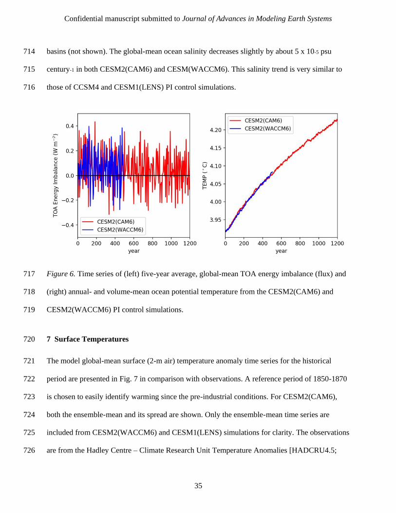
The impacts of these tunings were assessed in decadal to multi-decadal length simulations prior 697
to the start of the main PI control simulations. Figure 6 (left panel) shows the time series of the 698
global-mean TOA energy imbalances (fluxes) for the two control simulations where the 699
imbalances are +0.05 and +0.06 W m-2 for CESM2(CAM6) and CESM2(WACCM6), 700
respectively, averaged over their integration lengths. These imbalances are +0.03 W m-2 during 701
the last 500 years of CESM2(CAM6) and +0.06 W m-2 during the last 200 years of 702
CESM2(WACCM6). While these TOA imbalances are much smaller than the imbalance of 703
about –0.15 W m-2 in CCSM4 [Gent et al., 2011], they are larger than the exceptionally small 704
TOA imbalance of near-zero in the CESM1(LENS) control simulation. In both CESM2(CAM6) 705
and CESM2(WACCM6) control simulations, this energy gain is solely reflected in the ocean 706
model, as the land and sea-ice components show minor energy losses. The global-mean energy 707
gain by the ocean model is about 0.07 W m-2 during the last 500 years of CESM2(CAM6) and 708
about 0.10 W m-2 during the last 200 years of CESM2(WACCM6). As a result, the global-mean 709
ocean potential temperature (Fig. 6, right panel) increases from its initial value of 3.92°C to 710
about 4.23°C by year 1200 in CESM2(CAM6). Similarly, it increases from 3.92°C to about 711
4.08°C in CESM2(WACCM6). Although the details of the depth ranges and magnitudes of this 712
warming differ across the ocean basins, depths below about 2 km show warming in all major 713
Confidential manuscript submitted to Journal of Advances in Modeling Earth Systems
35
basins (not shown). The global-mean ocean salinity decreases slightly by about 5 x 10⁻⁵ psu 714
century-1 in both CESM2(CAM6) and CESM(WACCM6). This salinity trend is very similar to 715
those of CCSM4 and CESM1(LENS) PI control simulations. 716
Figure 6. Time series of (left) five-year average, global-mean TOA energy imbalance (flux) and 717
(right) annual- and volume-mean ocean potential temperature from the CESM2(CAM6) and 718
CESM2(WACCM6) PI control simulations. 719
7 Surface Temperatures 720
The model global-mean surface (2-m air) temperature anomaly time series for the historical 721
period are presented in Fig. 7 in comparison with observations. A reference period of 1850-1870 722
is chosen to easily identify warming since the pre-industrial conditions. For CESM2(CAM6), 723
both the ensemble-mean and its spread are shown. Only the ensemble-mean time series are 724
included from CESM2(WACCM6) and CESM1(LENS) simulations for clarity. The observations 725
are from the Hadley Centre – Climate Research Unit Temperature Anomalies [HADCRU4.5; 726
Confidential manuscript submitted to Journal of Advances in Modeling Earth Systems
36
Jones et al., 2012]; the Goddard Institute for Space Studies Surface Temperature Analysis 727
[GISTEMP; Lenssen et al., 2019]; and the National Oceanic and Atmospheric Administration 728
merged land-ocean global surface temperature analysis [NOAAGlobalTemp; Vose et al., 2012]. 729
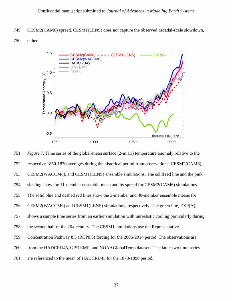
In general, the CESM2(WACCM6) time series tend to be slightly warmer than those of 730
CESM2(CAM6). Both sets of simulations capture the observed low-frequency variability, and 731
the observations are usually within the ensemble spread of CESM2(CAM6) simulations with a 732
few notable exceptions. One such example is the dip around 1910 evident in observations, but 733
absent in model simulations. This discrepancy may be related to incorrect and / or missing 734
representations of impacts of volcanic eruptions in both models and observations during the 735
1900-1910 period. Another major discrepancy is seen during the 2000-2014 period with model 736
ensemble-mean temperature anomalies being warmer than observed by about 0.2°C and 0.4°C at 737
the end of the integration period in CESM2(CAM6) and CESM2(WACCM6) simulations, 738
respectively. Although the warming trends between 1975-2000 are comparable between these 739
two model simulations and observations, no CESM2 ensemble member is able to capture the 740
observed slowdown in the warming trend during roughly 2000-2012. This is not surprising as 741
internal variability as well as anthropogenic and natural forcings are known to play a role in the 742
creation of this decadal-scale slowdown [e.g., Solomon et al., 2010; Kaufmann et al., 2011; 743
Kosaka and Xie, 2013; Meehl et al., 2014; Deser et al., 2017]. Indeed, as discussed in Meehl et 744
al. [2014], a much larger ensemble than presently used is needed as such a slowdown is present 745
only in a very small fraction of the available CMIP5 simulations (10 out of 262). In comparison 746
to CESM2 simulations and observations, CESM1(LENS) ensemble-mean time series show 747
generally colder temperature anomalies, usually remaining below or near the lower extent of the 748
Confidential manuscript submitted to Journal of Advances in Modeling Earth Systems
37
CESM2(CAM6) spread. CESM1(LENS) does not capture the observed decadal-scale slowdown, 749
either. 750
Figure 7. Time series of the global-mean surface (2-m air) temperature anomaly relative to the 751
respective 1850-1870 averages during the historical period from observations, CESM2(CAM6), 752
CESM2(WACCM6), and CESM1(LENS) ensemble simulations. The solid red line and the pink 753
shading show the 11-member ensemble-mean and its spread for CESM2(CAM6) simulations. 754
The solid blue and dashed red lines show the 3-member and 40-member ensemble means for 755
CESM2(WACCM6) and CESM1(LENS) simulations, respectively. The green line, EXP(A), 756
shows a sample time series from an earlier simulation with unrealistic cooling particularly during 757
the second half of the 20th century. The CESM1 simulations use the Representative 758
Concentration Pathway 8.5 (RCP8.5) forcing for the 2006-2014 period. The observations are 759
from the HADCRU45, GISTEMP, and NOAAGlobalTemp datasets. The latter two time series 760
are referenced to the mean of HADCRU45 for the 1870-1890 period. 761
Confidential manuscript submitted to Journal of Advances in Modeling Earth Systems
38
The 1985-2014 average SST (0-10 m average in the ocean) distributions from CESM2(CAM6), 762
CESM2(WACCM6), and CESM1(LENS) ensemble-means are presented in Fig. 8 in comparison 763
to the Extended Reconstructed Sea Surface Temperature version 5 dataset [ERSSTv5; Huang et 764
al., 2017]. There are two salient features in the figure, particularly evident in the model – 765
observations difference distributions. First, CESM2(CAM6) and CESM2(WACCM6) mean 766
SSTs are almost identical to each other. Second, both model SSTs are similarly warmer than 767
observations and those of CESM1(LENS). Indeed, CESM2(CAM6) and CESM2(WACCM6) 768
global-mean SSTs are warmer than observations by 0.39 and 0.33°C, respectively, while 769
CESM1(LENS) is colder than observations by 0.27°C. These global-mean differences essentially 770
reflect the SST differences in the corresponding PI control simulations from the ERSSTv5 771
dataset for the pre-industrial period, which are computed as 0.33°C for CESM2(CAM6), 0.18°C 772
for CESM2(WACCM6), and –0.18°C for CESM1(LENS) over 30-year periods close to the 773
mean initial start dates of the respective historical ensemble members. When root-mean-square 774
(rms) differences from observations are considered, both CESM2(CAM6) and 775
CESM2(WACCM6) have slight degradations of the mean SST simulations with rms differences 776
of 0.77 and 0.75°C, respectively, compared to 0.67°C for CESM1(LENS). The SST difference 777
distributions depict several persistent biases. The warm-cold SST difference dipole in the North 778
Atlantic associated with errors in the separation and path of the Gulf Stream – North Atlantic 779
Current system is present in all model simulations with comparable magnitudes. The warm 780
biases in the Eastern boundary upwelling regions, i.e., off the coasts of California, South 781
America, and South Africa, are more pronounced in CESM2(CAM6) and CESM2(WACCM6) 782
than in CESM1(LENS). These CESM2 biases are much larger in their magnitude (and spatial 783
extent) than the global- and time-mean SST differences between CESM2 and CESM1(LENS), so 784

Confidential manuscript submitted to Journal of Advances in Modeling Earth Systems
39
the larger CESM2 biases cannot be solely attributed to the warmer mean state of these 785
simulations. Reducing these upwelling-related biases has been rather challenging in 1° horizontal 786
resolution models. In CESM1, the upwelling biases were reduced due to more realistic wind 787

Confidential manuscript submitted to Journal of Advances in Modeling Earth Systems
40
stress curl in a model configuration with much higher horizontal resolutions in the ocean and 788
atmospheric models than used in the present simulations [Small et al., 2015]. 789
Figure 8. 1985-2014 average sea surface temperature (in °C) from (top) ERSST observations and 790
(left) model simulations. The right panels show the respective model minus observations 791
difference distributions. The model distributions represent full ensemble means. The global-792
Confidential manuscript submitted to Journal of Advances in Modeling Earth Systems
41
means for each panel and the root-mean-square error for the difference distributions are also 793
provided. 794
Seasonal-average surface (2-m) air temperature model minus observations differences over land 795
for December-January-February (DJF) and June-July-August (JJA) for the 1985-2014 period 796
from CESM2(CAM6), CESM2(WACCM6), and CESM1(LENS) are shown in Fig. 9. The 797
observations are from the Berkeley Earth Surface Temperatures dataset [BEST; Rohde et al., 798
2013]. As in the SST distributions, CESM2(CAM6) and CESM2(WACCM6) distributions are 799
very similar to each other and, on average, CESM2 is warmer than CESM1. Both the global 800
mean bias and rms error are appreciably lower in CESM2 than in CESM1 in all seasons. For 801
example, the DJF mean bias (rms error) has been reduced from –2.24°C (1.90°C) in 802
CESM1(LENS) to 0.89°C (1.51°C) and 0.67°C (1.38°C) in CESM2(CAM6) and 803
CESM2(WACCM6), respectively. In CESM2, there is a notably damped annual cycle – warm 804
biases in the winter season and cold biases in the summer season – in the northern high latitudes. 805
There is also a large summertime warm bias over the central United States, which partially 806
coincides with a dry bias (see Fig. 10), and may be related to the absence of propagating 807
mesoscale convective systems at the 1° model resolution. Another interesting bias is the warm 808
bias over Northeast India which exists in all seasons except for March-April-May (MAM) (not 809
shown). This region is among the most heavily irrigated regions in the world and previous 810
studies have shown that the irrigation-induced cooling is likely mitigating against climate 811
warming in this area [Thiery et al., 2020]. Though CESM2 includes active irrigation by default, 812
irrigation in India is applied mainly in the MAM season due to a limitation in the crop planting 813
date scheme that incorrectly results in crops being planted in the spring over India. In reality, 814
over much of Northern India, the two main cropping and irrigation seasons are in summer and in 815
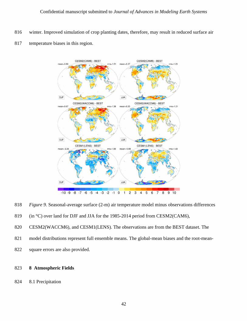
Confidential manuscript submitted to Journal of Advances in Modeling Earth Systems
42
winter. Improved simulation of crop planting dates, therefore, may result in reduced surface air 816
temperature biases in this region. 817
Figure 9. Seasonal-average surface (2-m) air temperature model minus observations differences 818
(in °C) over land for DJF and JJA for the 1985-2014 period from CESM2(CAM6), 819
CESM2(WACCM6), and CESM1(LENS). The observations are from the BEST dataset. The 820
model distributions represent full ensemble means. The global-mean biases and the root-mean-821
square errors are also provided. 822
8 Atmospheric Fields 823
8.1 Precipitation 824
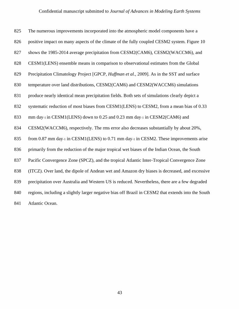
Confidential manuscript submitted to Journal of Advances in Modeling Earth Systems
43
The numerous improvements incorporated into the atmospheric model components have a 825
positive impact on many aspects of the climate of the fully coupled CESM2 system. Figure 10 826
shows the 1985-2014 average precipitation from CESM2(CAM6), CESM2(WACCM6), and 827
CESM1(LENS) ensemble means in comparison to observational estimates from the Global 828
Precipitation Climatology Project [GPCP, Huffman et al., 2009]. As in the SST and surface 829
temperature over land distributions, CESM2(CAM6) and CESM2(WACCM6) simulations 830
produce nearly identical mean precipitation fields. Both sets of simulations clearly depict a 831
systematic reduction of most biases from CESM1(LENS) to CESM2, from a mean bias of 0.33 832
mm day-1 in CESM1(LENS) down to 0.25 and 0.23 mm day-1 in CESM2(CAM6) and 833
CESM2(WACCM6), respectively. The rms error also decreases substantially by about 20%, 834
from 0.87 mm day-1 in CESM1(LENS) to 0.71 mm day-1 in CESM2. These improvements arise 835
primarily from the reduction of the major tropical wet biases of the Indian Ocean, the South 836
Pacific Convergence Zone (SPCZ), and the tropical Atlantic Inter-Tropical Convergence Zone 837
(ITCZ). Over land, the dipole of Andean wet and Amazon dry biases is decreased, and excessive 838
precipitation over Australia and Western US is reduced. Nevertheless, there are a few degraded 839
regions, including a slightly larger negative bias off Brazil in CESM2 that extends into the South 840
Atlantic Ocean. 841

Confidential manuscript submitted to Journal of Advances in Modeling Earth Systems
44
Figure 10. 1985-2014 average total precipitation (in mm day-1) from (top) GPCP observations 842
and (left) model simulations. The right panels show the respective model minus observations 843
difference distributions. The model distributions represent full ensemble means. The global-844
means for each panel and the root-mean-square error for the difference distributions are also 845
provided. 846

Confidential manuscript submitted to Journal of Advances in Modeling Earth Systems
45
8.2 Short-wave and long-wave cloud forcing 847
A dramatic improvement is seen in the radiative properties and, in particular, the time-averaged 848
short-wave cloud forcing (Fig. 11). In comparison to the Clouds and the Earth’s Radiant Energy 849
System – Energy Balanced and Filled [CERES-EBAF; Loeb et al., 2009] dataset, the reflective 850
biases of the clouds in CESM1(LENS) throughout the tropics over land and ocean, often in 851
excess of –30 W m-2, are substantially alleviated in both CESM2(CAM6) and 852
CESM2(WACCM6). This improvement is due to several changes in different cloud regimes. The 853
interaction of CLUBB with the CAM6 deep convective parameterization enabled a re-adjustment 854
of tropical deep convection over land to reduce biases. Net rms for shallow clouds is reduced 855
with CLUBB. At higher latitudes, low clouds were insufficiently bright in CESM1(LENS). 856
Changes in mixed-phase cloud properties in the MG2 microphysics scheme produce more 857
supercooled liquid water in CESM2 and result in more low clouds and more reflective clouds. 858
Quantitatively, the global-mean rms error is substantially reduced from about 14 W m-2 in 859
CESM1(LENS) to about 9.1 W m-2 in CESM2(CAM6) and 9.7 W m-2 in CESM2(WACCM6). 860
The subtropical stratocumulus regions show a few large-scale improvements. For the most part 861
however, deficiencies in cloud forcing seen in CESM1(LENS) are still seen in the 862
CESM2(CAM6) and CESM2(WACCM6) stratocumulus regions. 863
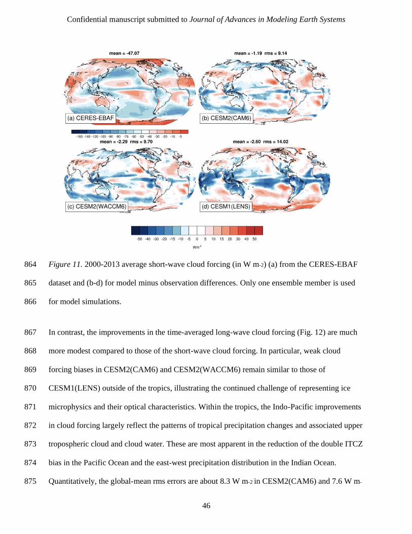
Confidential manuscript submitted to Journal of Advances in Modeling Earth Systems
46
Figure 11. 2000-2013 average short-wave cloud forcing (in W m-2) (a) from the CERES-EBAF 864
dataset and (b-d) for model minus observation differences. Only one ensemble member is used 865
for model simulations. 866
In contrast, the improvements in the time-averaged long-wave cloud forcing (Fig. 12) are much 867
more modest compared to those of the short-wave cloud forcing. In particular, weak cloud 868
forcing biases in CESM2(CAM6) and CESM2(WACCM6) remain similar to those of 869
CESM1(LENS) outside of the tropics, illustrating the continued challenge of representing ice 870
microphysics and their optical characteristics. Within the tropics, the Indo-Pacific improvements 871
in cloud forcing largely reflect the patterns of tropical precipitation changes and associated upper 872
tropospheric cloud and cloud water. These are most apparent in the reduction of the double ITCZ 873
bias in the Pacific Ocean and the east-west precipitation distribution in the Indian Ocean. 874
Quantitatively, the global-mean rms errors are about 8.3 W m-2 in CESM2(CAM6) and 7.6 W m-875
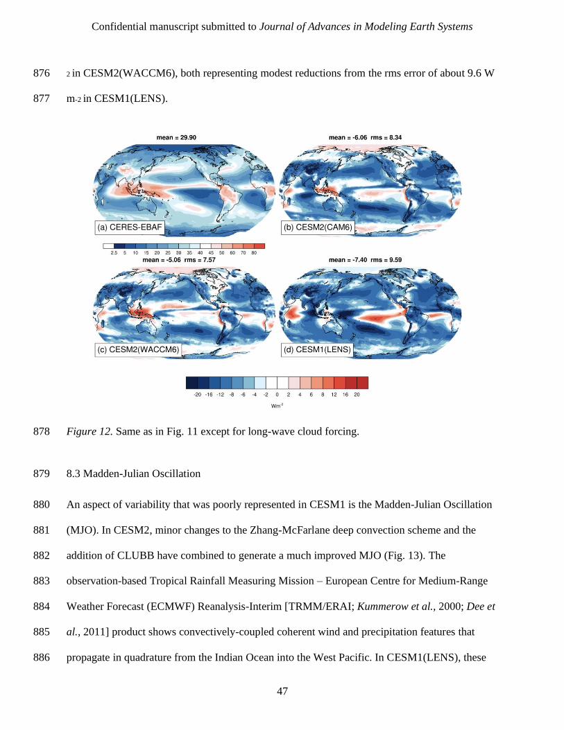
Confidential manuscript submitted to Journal of Advances in Modeling Earth Systems
47
2 in CESM2(WACCM6), both representing modest reductions from the rms error of about 9.6 W 876
m-2 in CESM1(LENS). 877
Figure 12. Same as in Fig. 11 except for long-wave cloud forcing. 878
8.3 Madden-Julian Oscillation 879
An aspect of variability that was poorly represented in CESM1 is the Madden-Julian Oscillation 880
(MJO). In CESM2, minor changes to the Zhang-McFarlane deep convection scheme and the 881
addition of CLUBB have combined to generate a much improved MJO (Fig. 13). The 882
observation-based Tropical Rainfall Measuring Mission – European Centre for Medium-Range 883
Weather Forecast (ECMWF) Reanalysis-Interim [TRMM/ERAI; Kummerow et al., 2000; Dee et 884
al., 2011] product shows convectively-coupled coherent wind and precipitation features that 885
propagate in quadrature from the Indian Ocean into the West Pacific. In CESM1(LENS), these 886
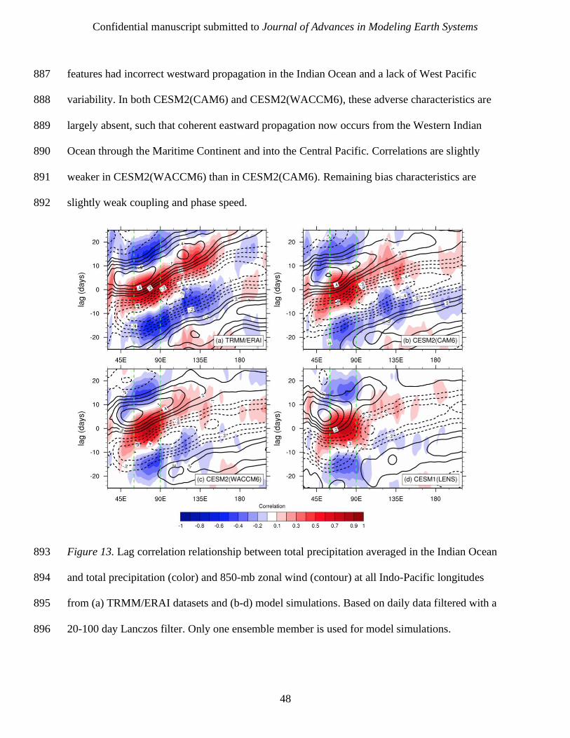
Confidential manuscript submitted to Journal of Advances in Modeling Earth Systems
48
features had incorrect westward propagation in the Indian Ocean and a lack of West Pacific 887
variability. In both CESM2(CAM6) and CESM2(WACCM6), these adverse characteristics are 888
largely absent, such that coherent eastward propagation now occurs from the Western Indian 889
Ocean through the Maritime Continent and into the Central Pacific. Correlations are slightly 890
weaker in CESM2(WACCM6) than in CESM2(CAM6). Remaining bias characteristics are 891
slightly weak coupling and phase speed. 892
Figure 13. Lag correlation relationship between total precipitation averaged in the Indian Ocean 893
and total precipitation (color) and 850-mb zonal wind (contour) at all Indo-Pacific longitudes 894
from (a) TRMM/ERAI datasets and (b-d) model simulations. Based on daily data filtered with a 895
20-100 day Lanczos filter. Only one ensemble member is used for model simulations. 896
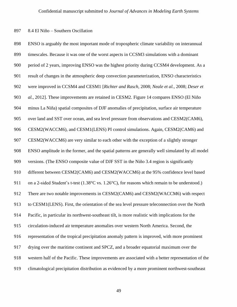
Confidential manuscript submitted to Journal of Advances in Modeling Earth Systems
49
8.4 El Niño – Southern Oscillation 897
ENSO is arguably the most important mode of tropospheric climate variability on interannual 898
timescales. Because it was one of the worst aspects in CCSM3 simulations with a dominant 899
period of 2 years, improving ENSO was the highest priority during CCSM4 development. As a 900
result of changes in the atmospheric deep convection parameterization, ENSO characteristics 901
were improved in CCSM4 and CESM1 [Richter and Rasch, 2008; Neale et al., 2008; Deser et 902
al., 2012]. These improvements are retained in CESM2. Figure 14 compares ENSO (El Niño 903
minus La Niña) spatial composites of DJF anomalies of precipitation, surface air temperature 904
over land and SST over ocean, and sea level pressure from observations and CESM2(CAM6), 905
CESM2(WACCM6), and CESM1(LENS) PI control simulations. Again, CESM2(CAM6) and 906
CESM2(WACCM6) are very similar to each other with the exception of a slightly stronger 907
ENSO amplitude in the former, and the spatial patterns are generally well simulated by all model 908
versions. (The ENSO composite value of DJF SST in the Niño 3.4 region is significantly 909
different between CESM2(CAM6) and CESM2(WACCM6) at the 95% confidence level based 910
on a 2-sided Student’s t-test (1.38°C vs. 1.26°C), for reasons which remain to be understood.) 911
There are two notable improvements in CESM2(CAM6) and CESM2(WACCM6) with respect 912
to CESM1(LENS). First, the orientation of the sea level pressure teleconnection over the North 913
Pacific, in particular its northwest-southeast tilt, is more realistic with implications for the 914
circulation-induced air temperature anomalies over western North America. Second, the 915
representation of the tropical precipitation anomaly pattern is improved, with more prominent 916
drying over the maritime continent and SPCZ, and a broader equatorial maximum over the 917
western half of the Pacific. These improvements are associated with a better representation of the 918
climatological precipitation distribution as evidenced by a more prominent northwest-southeast 919
Confidential manuscript submitted to Journal of Advances in Modeling Earth Systems
50
oriented SPCZ that is confined to the western Pacific and less of a double ITCZ structure as 920
indicated by the contours in the top row. The precipitation anomaly pattern in CESM2(CAM6) 921
and CESM2(WACCM6) also shows a stronger east-west Walker Circulation component, more in 922
line with observations, compared to the dominant narrow Hadley Circulation response in 923
CESM1(LENS). 924
Figure 14. Spatial composites of DJF ENSO anomalies of precipitation (top row; in mm day-1), 925
surface air temperature over land and SST over ocean (bottom row; color shading; in °C), and 926
sea level pressure (bottom row; contours; –16 to 16 hPa by 2 hPa with negative contours dashed) 927
from observations, CESM2(CAM6) PI control for years 100-1199, CESM2(WACCM6) PI 928
control for years 50-499, and CESM1(LENS) PI control for years 500-1599. The 6 mm day-1 929
DJF climatological mean precipitation contour is shown in black for each dataset in the top row. 930
The normalized December Niño 3.4 timeseries are used to composite all years greater than 1 931
standard deviation (El Niño) and all years less than –1 standard deviation (La Niña), and the 932
ENSO composite is formed by subtracting the La Niña composite from the El Niño composite. 933
Observations are from GPCP for precipitation (1979-2017), ERSSTv5 for SST (1920-2017), 934
Confidential manuscript submitted to Journal of Advances in Modeling Earth Systems
51
BEST for 2-m air temperature (1920-2017), and ECMWF Reanalysis for the 20th century 935
[ERA20C; Poli et al., 2016] combined with ERA-Interim [Berrisford et al., 2009] for sea level 936
pressure (1920-2017). 937
8.5 Stratospheric ozone 938
WACCM6 is able to accurately simulate the evolution of stratospheric ozone over the late 20th 939
century. In particular, WACCM6 can produce the halogen-induced ozone loss in the Southern 940
Hemisphere polar stratosphere in spring. This occurs due to the activation of chlorine and 941
bromine via heterogeneous chemistry on the surface of polar stratospheric cloud particles [WMO, 942
2010]. Figure 15 illustrates the annual evolution of the Southern Hemisphere polar cap Total 943
Column Ozone (TCO) in October. Coupled historical and AMIP-type simulations with 944
WACCM6 are able to broadly represent the ozone loss from the 1970s through 1990s. “Specified 945
Dynamics” (SD) simulations, wherein the model is constrained with MERRA-2 [Rienecker et 946
al., 2011] meteorology (SD-MERRA2), indicate that much of the variability in observations can 947
be explained by interannual variability of meteorology in the Southern Hemisphere polar vortex. 948
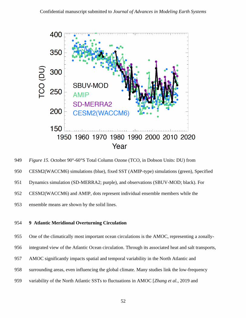
Confidential manuscript submitted to Journal of Advances in Modeling Earth Systems
52
Figure 15. October 90°-60°S Total Column Ozone (TCO, in Dobson Units: DU) from 949
CESM2(WACCM6) simulations (blue), fixed SST (AMIP-type) simulations (green), Specified 950
Dynamics simulation (SD-MERRA2; purple), and observations (SBUV-MOD; black). For 951
CESM2(WACCM6) and AMIP, dots represent individual ensemble members while the 952
ensemble means are shown by the solid lines. 953
9 Atlantic Meridional Overturning Circulation 954
One of the climatically most important ocean circulations is the AMOC, representing a zonally-955
integrated view of the Atlantic Ocean circulation. Through its associated heat and salt transports, 956
AMOC significantly impacts spatial and temporal variability in the North Atlantic and 957
surrounding areas, even influencing the global climate. Many studies link the low-frequency 958
variability of the North Atlantic SSTs to fluctuations in AMOC [Zhang et al., 2019 and 959
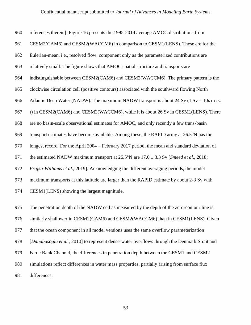
Confidential manuscript submitted to Journal of Advances in Modeling Earth Systems
53
references therein]. Figure 16 presents the 1995-2014 average AMOC distributions from 960
CESM2(CAM6) and CESM2(WACCM6) in comparison to CESM1(LENS). These are for the 961
Eulerian-mean, i.e., resolved flow, component only as the parameterized contributions are 962
relatively small. The figure shows that AMOC spatial structure and transports are 963
indistinguishable between CESM2(CAM6) and CESM2(WACCM6). The primary pattern is the 964
clockwise circulation cell (positive contours) associated with the southward flowing North 965
Atlantic Deep Water (NADW). The maximum NADW transport is about 24 Sv (1 Sv = 106 m3 s-966
1) in CESM2(CAM6) and CESM2(WACCM6), while it is about 26 Sv in CESM1(LENS). There 967
are no basin-scale observational estimates for AMOC, and only recently a few trans-basin 968
transport estimates have become available. Among these, the RAPID array at 26.5°N has the 969
longest record. For the April 2004 – February 2017 period, the mean and standard deviation of 970
the estimated NADW maximum transport at 26.5°N are 17.0 ± 3.3 Sv [Smeed et al., 2018; 971
Frajka-Williams et al., 2019]. Acknowledging the different averaging periods, the model 972
maximum transports at this latitude are larger than the RAPID estimate by about 2-3 Sv with 973
CESM1(LENS) showing the largest magnitude. 974
The penetration depth of the NADW cell as measured by the depth of the zero-contour line is 975
similarly shallower in CESM2(CAM6) and CESM2(WACCM6) than in CESM1(LENS). Given 976
that the ocean component in all model versions uses the same overflow parameterization 977
[Danabasoglu et al., 2010] to represent dense-water overflows through the Denmark Strait and 978
Faroe Bank Channel, the differences in penetration depth between the CESM1 and CESM2 979
simulations reflect differences in water mass properties, partially arising from surface flux 980
differences. 981
Confidential manuscript submitted to Journal of Advances in Modeling Earth Systems
54
The counterclockwise (negative contours) circulation region in the abyssal ocean below the 982
NADW cell represents the northward flowing Antarctic Bottom Water (AABW). In comparison 983
to very limited observational estimates, all the simulations suffer from a chronic bias of very 984
anemic AABW transport due to too weak AABW formation, with CESM2(CAM6) and 985
CESM2(WACCM6) showing only a marginally broader and stronger AABW cell than in 986
CESM1(LENS). The observational range for the AABW transport into the Atlantic basin is 987
about 1-5 Sv at 24.5°N based on sparse datasets dating back to 1957 [Frajka-Williams et al., 988
2011]. Both CESM2 simulations have a maximum transport of about 0.5 Sv, compared to near 989
zero in CESM1(LENS). Such weak deep overturning circulations lead to weak ventilation at 990
depth evident in tracer distributions particularly in the North Pacific, compared to available 991
observations (not shown). 992
Figure 16. 1995-2014 average Eulerian-mean Atlantic meridional overturning circulation (in Sv) 993
from (left) CESM2(CAM6), (middle) CESM2(WACCM6), and (right) CESM1(LENS). The 994
model distributions represent full ensemble means. The positive and negative contours indicate 995
clockwise and counter-clockwise circulations, respectively. 996
10 Sea-Ice and Land-Ice Fields 997
10.1 Sea-ice thickness and extent 998

Confidential manuscript submitted to Journal of Advances in Modeling Earth Systems
55
The annual-mean sea-ice thickness and extent are shown in Fig. 17, averaged for 1979-2014. For 999
the Arctic, sea-ice in both CESM2 simulations is thinner than in CESM1(LENS), which has a 1000
total annual-mean Arctic ice volume of 28.9x10³ km3. The sea-ice is considerably thicker in the 1001
simulations with CESM2(WACCM6) than with CESM2(CAM6), with the respective total 1002
annual-mean Arctic ice volumes of 21.4x10³ and 15.4x10³ km3. The CESM2(WACCM6) 1003
simulations agree well with observationally-based estimates from the Pan-Arctic Ice Ocean 1004
Modeling and Assimilation System [PIOMAS; Schweiger et al., 2011], which simulates a 1979-1005
2014 average Arctic ice volume of 20.2x10³ km3. The thicker sea-ice in CESM2(WACCM6) is 1006
related to liquid Arctic clouds, which are thicker as a result of increased aerosol concentrations 1007
predicted from the interactive chemistry module [Gettelman et al., 2019a]. Specifically, the 1008
interactive oxidants with full chemistry in CESM2(WACCM6) mean that aerosols will evolve 1009
differently. Because the aerosols are not produced locally in remote regions such as the Arctic, 1010
the increase in aerosol concentrations over the Arctic is due to a lengthening of the aerosol 1011
lifetime. The anti-correlation between aerosols and oxidants is meteorologically dependent, and 1012
so may not be seen in monthly average oxidants fields used in CESM2(CAM6), leading to a 1013
different aerosol evolution, particularly in such remote areas. The differences in sea-ice thickness 1014
between the two model configurations have consequences for the annual cycle of ice extent. In 1015
particular, with the thin ice bias in the CESM2(CAM6) simulations, more melting occurs during 1016
the summer months, with a resulting low summer ice extent as compared to satellite passive-1017
microwave observations (Fig. 17g). In contrast, CESM2(WACCM6) and CESM1(LENS) have 1018
an excellent simulation of summer ice extent compared to observations. In both CESM2(CAM6) 1019
and CESM2(WACCM6) simulations, the ice extent is low in winter compared to observations. 1020
Confidential manuscript submitted to Journal of Advances in Modeling Earth Systems
56
This is in contrast to CESM1(LENS) which simulates a winter ice extent that is in very good 1021
agreement with observations. 1022
In the Southern Hemisphere, the sea-ice is nearly identical in CESM2(CAM6) and 1023
CESM2(WACCM6), both somewhat thinner than the sea-ice simulated in CESM1(LENS). As in 1024
observations, a primarily seasonal ice pack is present and the ice remains thinner than 1 m in the 1025
annual mean over most of the sea-ice domain for all model versions. Sea-ice thicker than 1 m 1026
forms in the Amundsen/Bellingshausen and Weddell Seas. This is in reasonable agreement with 1027
the limited in-situ ice thickness observations [Worby et al., 2008]. The ice extent annual cycle is 1028
also reasonably well simulated in both CESM2 simulations. The maximum simulated ice cover is 1029
biased low by about 1.6x10⁶ km2, and the ice melt-back is delayed by about one month relative 1030
to observations but reaches a similar minimum ice cover in February. This is in contrast to 1031
CESM1(LENS), which has a good simulation of the winter maximum ice extent but retains too 1032
much ice at the summer minimum. 1033
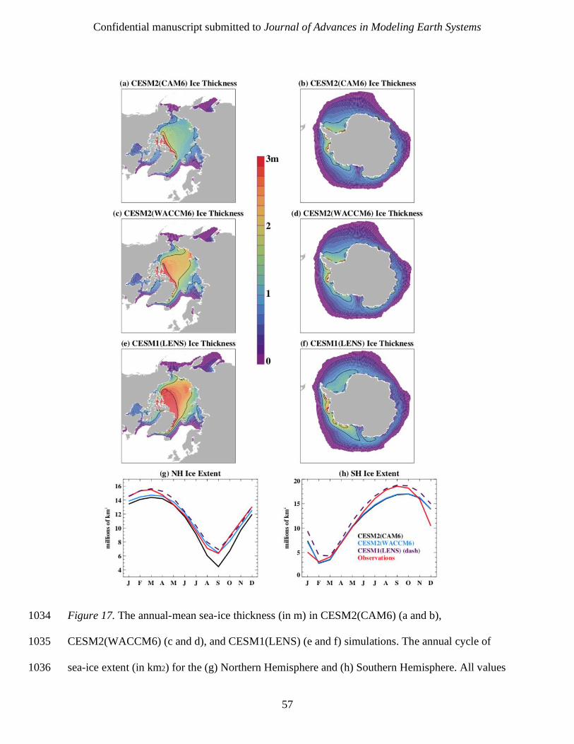
Confidential manuscript submitted to Journal of Advances in Modeling Earth Systems
57
Figure 17. The annual-mean sea-ice thickness (in m) in CESM2(CAM6) (a and b), 1034
CESM2(WACCM6) (c and d), and CESM1(LENS) (e and f) simulations. The annual cycle of 1035
sea-ice extent (in km2) for the (g) Northern Hemisphere and (h) Southern Hemisphere. All values 1036
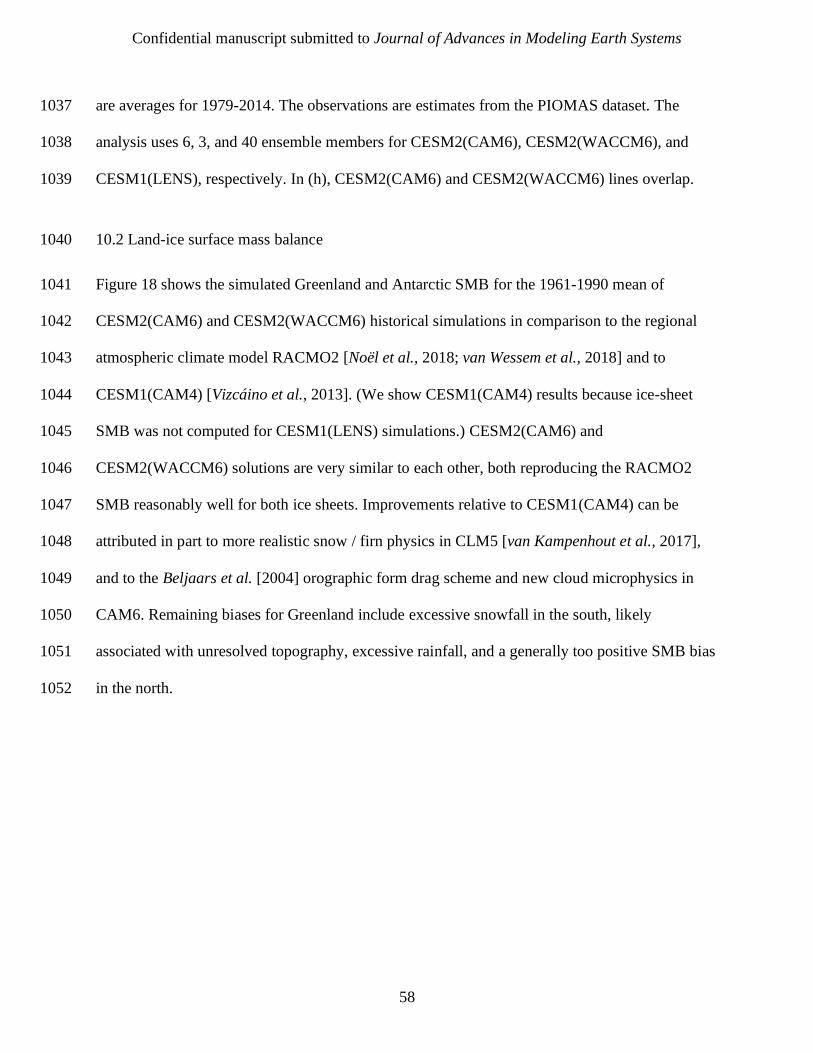
Confidential manuscript submitted to Journal of Advances in Modeling Earth Systems
58
are averages for 1979-2014. The observations are estimates from the PIOMAS dataset. The 1037
analysis uses 6, 3, and 40 ensemble members for CESM2(CAM6), CESM2(WACCM6), and 1038
CESM1(LENS), respectively. In (h), CESM2(CAM6) and CESM2(WACCM6) lines overlap. 1039
10.2 Land-ice surface mass balance 1040
Figure 18 shows the simulated Greenland and Antarctic SMB for the 1961-1990 mean of 1041
CESM2(CAM6) and CESM2(WACCM6) historical simulations in comparison to the regional 1042
atmospheric climate model RACMO2 [Noël et al., 2018; van Wessem et al., 2018] and to 1043
CESM1(CAM4) [Vizcáino et al., 2013]. (We show CESM1(CAM4) results because ice-sheet 1044
SMB was not computed for CESM1(LENS) simulations.) CESM2(CAM6) and 1045
CESM2(WACCM6) solutions are very similar to each other, both reproducing the RACMO2 1046
SMB reasonably well for both ice sheets. Improvements relative to CESM1(CAM4) can be 1047
attributed in part to more realistic snow / firn physics in CLM5 [van Kampenhout et al., 2017], 1048
and to the Beljaars et al. [2004] orographic form drag scheme and new cloud microphysics in 1049
CAM6. Remaining biases for Greenland include excessive snowfall in the south, likely 1050
associated with unresolved topography, excessive rainfall, and a generally too positive SMB bias 1051
in the north. 1052

Confidential manuscript submitted to Journal of Advances in Modeling Earth Systems
59
Figure 18. Surface mass balance (SMB in mm water equivalent yr-1) of the Greenland ice sheet 1053
(top row) and Antarctic ice sheet (bottom row) from statistically downscaled output of the 1054
regional atmospheric climate model RACMO2.3p2, and from CESM2(CAM6), 1055
CESM2(WACCM6), and CESM1(CAM4). The CESM results are from historical simulations 1056
averaged over 1961-1990, with eleven ensemble members for CESM2(CAM6), three members 1057
for CESM2(WACCM6), and one member for CESM1(CAM4). For Greenland, CESM2 SMB 1058
has been downscaled using multiple elevation classes to a 5-km grid for CESM1(CAM4) and to 1059
a 4-km CISM grid for both versions of CESM2. For Antarctica, both CESM1 and CESM2 SMB 1060
are shown on the land model grid without downscaling. RACMO2.3p2 data are averaged over 1061
1961-1990 for Greenland [Noël et al., 2018] and over 1979-2010 for Antarctica [van Wessem et 1062
al., 2018] at a resolution of 11 and 27 km, respectively. 1063
Confidential manuscript submitted to Journal of Advances in Modeling Earth Systems
60
11 Land Fields 1064
The land model variables are assessed with the International Land Model Benchmarking 1065
[ILAMBv2.1; Collier et al., 2018] package. The ILAMBv2 used here integrates analysis for 30 1066
variables evaluated against more than 60 data products. ILAMB package results include 1067
statistics, maps, time series, and metrics for relative bias, rms error, seasonal cycle phase, spatial 1068
distribution, and interannual variability, as well as variable-to-variable assessments that evaluate 1069
functional relationships between variables. ILAMB summary diagrams, which integrate scores 1070
across several datasets and metrics for each variable and variable-to-variable comparisons, are 1071
shown in Fig. 19 for three ensemble members each of CESM1(LENS) and CESM2(CAM6) – 1072
CESM2(WACCM6) results are very similar to those of CESM2(CAM6). For most variables 1073
assessed, CESM2(CAM6) better matches the observations than CESM1(LENS). Except for 1074
precipitation, all the land climate variables (shown in grey in the left panel of Fig. 19) show 1075
modest improvement, indicating an improved surface climate simulation in CESM2(CAM6) due 1076
to a combination of improvements in CAM6 and CLM5. The land carbon, water, and energy 1077
variable improvements are also seen in land-only simulations forced with historical climate 1078
reconstructions (not shown, see Lawrence et al. [2019] for detailed assessment), which suggests 1079
that improvements in these variables are predominantly a result of CLM5 physics and 1080
biogeochemistry model development rather than an outcome of a better-simulated surface 1081
climate in CESM2(CAM6). The consistently improved variable-to-variable scores suggests 1082
improved process-representation in CLM5. These functional relationship scores are improved 1083
even for comparisons involving a mean quantity that is slightly degraded in CESM2(CAM6) – 1084
e.g., land precipitation is slightly degraded, but precipitation versus gross primary productivity 1085
and precipitation versus burned area are improved. This result supports the interpretation that the 1086

Confidential manuscript submitted to Journal of Advances in Modeling Earth Systems
61
improvements derive mainly from CLM5 developments. Insight into the sources of improvement 1087
is provided in Lawrence et al. [2019] and Wieder et al. [2019]. A caveat here is that ILAMB 1088
results should be interpreted carefully and that an improvement or degradation in a particular 1089
ILAMB variable should not be overly interpreted as indicative of whether or not results that are 1090
dependent on that variable are reliable or not [see Lawrence et al., 2019 and Bonan et al., 2019]. 1091
For example, soil carbon is degraded according to the ILAMB metric, but other aspects of soil 1092
carbon such as the soil carbon turnover time appear to be improved [Lawrence et al., 2019], 1093
potentially reflecting a lack of consistency across observational datasets or a limitation in the 1094
applied ILAMB metric. A note of caution on the soil carbon field in CESM2 is that due to an 1095
error in the model spinup process, unrealistically large soil carbon stocks are seen for some high-1096
latitude grid cells where vegetation does not survive the cold climate (e.g., Canadian 1097
Archipelago). For these grid cells, the spinup process was supposed to set soil carbon stocks to 1098
near zero, but due to very small but non-zero vegetation stocks, the soil carbon stocks were not 1099
set to zero as intended. Model users can resolve this problem (which was fixed in CESM2.1.1) 1100
by screening out large soil carbon stocks when vegetation carbon is zero. 1101
Confidential manuscript submitted to Journal of Advances in Modeling Earth Systems
62
Figure 19. ILAMB summary diagrams for three ensemble members each of CESM1(LENS) and 1102
CESM2(CAM6) historical simulations. The left panel shows the single-variable assessment 1103
summary for land variables. The upper part of the right panel shows assessment of the land 1104
forcing variables as simulated by the atmosphere model. The lower part of the right panel shows 1105
a variable-to-variable comparison summary. See Collier et al. [2018] for details on all metrics. 1106
Full ILAMB package results for both coupled and land-only simulations are available at 1107
http://www.cesm.ucar.edu/experiments/cesm2.0/land/diagnostics/clm_diag_ILAMB.html. 1108
One of the clearest improvements in CESM2 and CLM5 is the simulated global land carbon 1109
accumulation trends. CESM1/CLM4 produced an unrealistically strong nutrient limitation on 1110
photosynthesis, which limited the capacity in CESM1 for carbon uptake in response to increases 1111
in atmospheric CO2 concentrations. Consequently, in CESM1 land-use and land-cover change 1112
Confidential manuscript submitted to Journal of Advances in Modeling Earth Systems
63
carbon loss fluxes dominate over the CO2 fertilization response, and CESM1 simulates an 1113
accumulated carbon loss over the period 1960 to 2004, whereas the observationally-based 1114
estimates indicate a carbon gain of ~40 PgC (Fig. 20). In CESM2(CAM6) and 1115
CESM2(WACCM6), the CO2 fertilization response appears to be more reasonable and, when 1116
this is combined with updates to the land-use and land-cover change carbon fluxes, results in a 1117
late 20th century accumulated carbon trend that agrees well with observationally-based estimates. 1118
Further discussion on the source of improvement for this feature of CESM2, which is also seen 1119
in land-only simulations, is provided in Lawrence et al. [2019], Wieder et al. [2019], and Bonan 1120
et al. [2019]. In addition to the improved accumulated carbon, CESM2 simulations also show 1121
evidence of considerable improvements in the amplitude of the annual cycle of net ecosystem 1122
exchange, especially at northern high latitudes (see Carbon Dioxide variable metrics in Fig. 19), 1123
which translate to improved annual cycle amplitudes of atmospheric CO2 concentrations in 1124
emissions-driven simulations. 1125

Confidential manuscript submitted to Journal of Advances in Modeling Earth Systems
64
Figure 20. Land carbon accumulation for the period 1960-2014 for 3 historical ensemble 1126
members of CESM2(CAM6), CESM2(WACCM6), and CESM1(LENS) along with 1127
observationally-based estimates. The latter are from the Global Carbon Project [Le Quéré et al., 1128
2016]. Grey shading shows uncertainty range for the observational estimates, using an 1129
uncertainty of 0.8 Pg C yr-1 and calculated assuming that the errors are additive in time as in 1130
Koven et al. [2013]. 1131
12 Equilibrium Climate Sensitivity and Transient Climate Response 1132
An important emergent property of the coupled model is its Equilibrium Climate Sensitivity 1133
[ECS; e.g., Stocker et al., 2013], defined as the equilibrium change in global-mean surface 1134
temperature (SST over the ice-free oceans and a radiative temperature over land and sea-ice) 1135
after a doubling of CO2 concentration. ECS can be estimated using a slab ocean model (SOM) 1136
configuration, because 1) such a configuration equilibrates much faster compared to one with a 1137
full-depth ocean model (about 50 vs. > 1000 years), and 2) ECS values obtained with a SOM 1138
Confidential manuscript submitted to Journal of Advances in Modeling Earth Systems
65
versus a full-depth ocean component are comparable to each other [Danabasoglu and Gent, 1139
2009]. Therefore, SOM configurations are used here to estimate the ECS of both model 1140
configurations. The control SOM experiments use a pre-industrial value of CO2 set at 280 ppmv. 1141
These respective control simulations are compared with a second set of SOM experiments in 1142
which the CO2 concentration is instantaneously doubled to 560 ppmv (2xCO2). All SOM 1143
experiments are integrated long enough to ensure that global-mean surface temperature has 1144
equilibrated and TOA radiative imbalances are near zero. Differencing the equilibrated surface 1145
temperatures between the respective control and 2xCO2 experiments, the ECS values are 1146
computed as 5.3°C for CESM2(CAM6) [Gettelman et al., 2019b] and 5.1°C for 1147
CESM2(WACCM6). These values represent significant increases from an ECS of around 4.0°C 1148
in the SOM version of CESM1(CAM5) [Gettelman et al., 2012]. 1149
Values of climate sensitivity derived from the first 150 years of fully-coupled 4xCO2 runs using 1150
the Gregory method [so called Effective Climate Sensitivity; Gregory et al., 2004] are 5.3°C for 1151
CESM2(CAM6) and 4.8°C for CESM2(WACCM6) compared to 4.3°C in CESM1(CAM5) 1152
obtained with the same method [Meehl et al., 2013]. However, this level of relatively good 1153
agreement with the above SOM-based estimates of ECS is deceptive, because the Gregory 1154
method estimate of climate sensitivity for CESM2 is highly sensitive to the number of simulation 1155
years used in the calculation, due to nonlinearities in the relationship between TOA energy 1156
imbalance and temperature, with larger estimates of climate sensitivity as more years are used. 1157
The evolution of CESM2's climate sensitivity through several development versions of the 1158
model is examined in detail in Gettelman et al. [2019b]. Both of these studies suggest that the 1159
increased climate sensitivity in CESM2 has arisen from a combination of relatively small 1160
changes to cloud microphysics and boundary layer parameters as well as from land parameter 1161

Confidential manuscript submitted to Journal of Advances in Modeling Earth Systems
66
changes that were introduced late in the development process, along with the introduction of 1162
more realistic clouds with CLUBB and MG2. 1163
Another important emergent property of the coupled model is its Transient Climate Response 1164
(TCR). It is calculated from a pair of fully coupled simulations: a control simulation, again 1165
usually for PI conditions, and a 1% per year CO2 concentration increase simulation. Following 1166
the ESMValTool [Eyring et al., 2020] procedure, TCR in CESM2 is calculated as the difference 1167
of the 20-year average (years 60-79) global mean surface temperature, centered around the time 1168
of CO2 doubling at about year 70, from the 140-year linear trend (fit) of the corresponding PI 1169
control, overlapping the 1% per year CO2 increase run. The TCR values are obtained as 2.0°C for 1170
CESM2(CAM6) and 1.9°C for CESM2(WACCM6). These values are very comparable to a TCR 1171
value of 2.3°C for CESM1(CAM5) reported by Meehl et al. [2013]. Processes leading to 1172
CESM2’s TCR value are being investigated. Preliminary analysis suggests that, in CESM2, 1173
while tropics and the Southern Ocean warm faster, the Northern Hemisphere at mid- and high-1174
latitudes warms at a slower rate, in comparison to CESM1. 1175
It is important to stress that all estimates of ECS and TCR are subject to substantial uncertainties 1176
arising from the details of the calculation procedures. These uncertainties include the selection of 1177
reference periods for the PI simulations, the length of the averaging periods, and whether 1178
detrending is applied or not. For the above CESM values, such details may result in 0.1-0.2°C 1179
differences. 1180
13 Summary and Discussion 1181
The new version of the Community Earth System Model, CESM2, contains many substantial 1182
science and infrastructure improvements and capabilities. The CESM project is contributing 1183
Confidential manuscript submitted to Journal of Advances in Modeling Earth Systems
67
simulations to the CMIP6 effort with two CESM2 model configurations differing only in their 1184
atmospheric components. While one configuration uses the low-top CAM6, CESM2(CAM6), the 1185
other employs WACCM6 with its high-top and comprehensive chemistry, CESM2(WACCM6). 1186
Both configurations use the same nominal 1° horizontal resolution. A noteworthy new approach 1187
in CESM2 is that CESM2(WACCM6) PI and historical simulations were performed first to 1188
obtain some of the necessary forcing datasets to run the corresponding CESM2(CAM6) 1189
simulations. This was critical to ensure that, for the first time for CESM, a physically consistent 1190
pair of low- and high-top atmospheric models are used. This manuscript documents the CESM2 1191
development process and evaluates solutions from the 1200-year CESM2(CAM6) and 500-year 1192
CESM2(WACCM6) PI control integrations and from the subsequent historical simulations. The 1193
focus has been primarily on the historical simulations, as they can be more easily and directly 1194
compared with modern observations. 1195
The new developments and capabilities in CESM2 result in many improvements in solutions in 1196
comparison to available observations and those of CESM1. These improvements include: major 1197
reductions in the tropical wet biases of the Indian Ocean, the SPCZ, and the Atlantic ITCZ, 1198
generally with less of a double ITCZ structure in both the Pacific and Atlantic Basins; reductions 1199
in the dipole of Andean wet and Amazon dry biases as well as in Australian and Western US 1200
excessive precipitation biases; substantial reductions in the reflective biases of the clouds 1201
throughout the tropics; a much better representation of MJO characteristics with coherent 1202
eastward propagation of wind and precipitation anomalies; more realistic representation of the 1203
northwest – southeast tilt of the sea level pressure anomaly teleconnection patterns associated 1204
with ENSO over the North Pacific; a global land carbon accumulation trend that matches the 1205
observationally-based trend remarkably well; and better representation of the SMB for both the 1206
Confidential manuscript submitted to Journal of Advances in Modeling Earth Systems
68
Greenland and Antarctic ice sheets. An important finding is that CESM2(CAM6) and 1207
CESM2(WACCM6) historical simulations produce solutions that are very similar to each other 1208
in most variables. So, these improvements are present in both sets of simulations. An exception 1209
is the Arctic sea-ice thickness with CESM2(WACCM6) showing thicker sea-ice than in 1210
CESM2(CAM6) in better agreement with observations. The thicker sea-ice in 1211
CESM2(WACCM6) is related to liquid Arctic clouds, which are thicker as a result of increased 1212
aerosol concentrations predicted from the interactive chemistry module. 1213
Figure 21 presents a summary analysis comparing CESM2 solutions to those of CESM1(LENS). 1214
The figure shows mean pattern correlations across climatological mean, seasonal contrasts (JJA-1215
DJF), and ENSO teleconnections for the first three ensemble members of CESM2(CAM6), 1216
CESM2(WACCM6), and CESM1(LENS) historical simulations for 11 atmospheric fields with 1217
respect to many observational-based datasets. Indeed, CESM2 simulations have notable 1218
improvements in many of the metrics considered here compared to those of CESM1(LENS). 1219
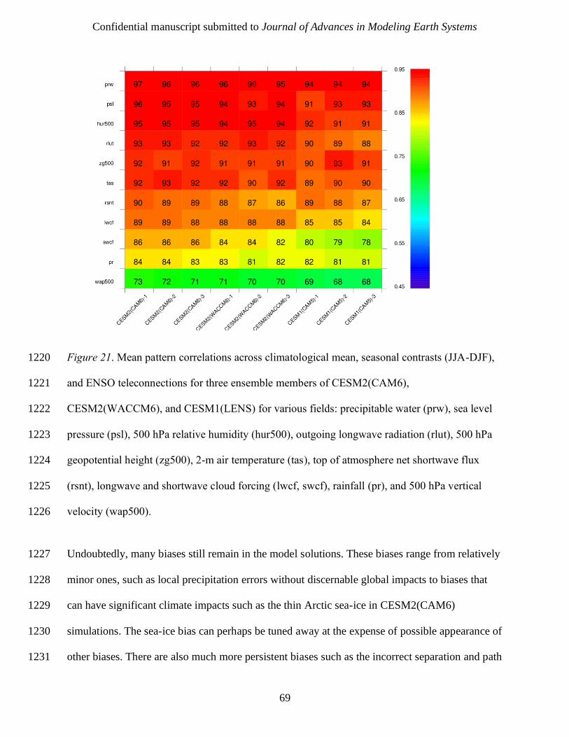
Confidential manuscript submitted to Journal of Advances in Modeling Earth Systems
69
Figure 21. Mean pattern correlations across climatological mean, seasonal contrasts (JJA-DJF), 1220
and ENSO teleconnections for three ensemble members of CESM2(CAM6), 1221
CESM2(WACCM6), and CESM1(LENS) for various fields: precipitable water (prw), sea level 1222
pressure (psl), 500 hPa relative humidity (hur500), outgoing longwave radiation (rlut), 500 hPa 1223
geopotential height (zg500), 2-m air temperature (tas), top of atmosphere net shortwave flux 1224
(rsnt), longwave and shortwave cloud forcing (lwcf, swcf), rainfall (pr), and 500 hPa vertical 1225
velocity (wap500). 1226
Undoubtedly, many biases still remain in the model solutions. These biases range from relatively 1227
minor ones, such as local precipitation errors without discernable global impacts to biases that 1228
can have significant climate impacts such as the thin Arctic sea-ice in CESM2(CAM6) 1229
simulations. The sea-ice bias can perhaps be tuned away at the expense of possible appearance of 1230
other biases. There are also much more persistent biases such as the incorrect separation and path 1231
Confidential manuscript submitted to Journal of Advances in Modeling Earth Systems
70
of the Gulf Stream – North Atlantic Current system, with accompanying large SST and surface 1232
salinity biases. This latter class of biases can have significant climate impacts as well, but no 1233
robust remedy exists to alleviate them in non-eddy-permitting / -resolving ocean models usually 1234
used in climate simulations. 1235
The path to finalizing a CESM2 version that produced acceptable simulations took much longer 1236
than anticipated. The process was hindered particularly by two major unacceptable features in 1237
simulations. The first concerned formation of unrealistically extensive sea-ice cover over the 1238
Labrador Sea region in PI control simulations. Unfortunately, extensive analysis of simulations 1239
did not reveal a particular process (or processes) as the culprit. To avoid further delays, a 1240
practical approach was adopted that involved performing several member ensemble simulations 1241
which differed at round-off levels in their atmospheric potential temperature initial conditions, 1242
and then using one of the members without an extensive Labrador Sea ice cover to provide the 1243
ocean and sea-ice initial conditions. The second issue was that the global-mean surface 1244
temperature time series in historical simulations showed a substantial and unrealistic cooling, 1245
particularly during the second half of the 20th century, with end-of-the-century temperatures 1246
being colder than in the 1850s. Adoption of updated CMIP6 emissions datasets, along with 1247
several modifications in the aerosol – cloud interaction processes based on observational data 1248
from recent volcanic sulfur emission events, resulted in surface temperature time series that 1249
evolve realistically during the historical period. Nevertheless, there are several discrepancies in 1250
the details of the modeled and observed time series. For example, the model surface temperatures 1251
are warmer in the early part of the 21st century than in observations by 0.2 and 0.4°C in 1252
CESM2(CAM6) and CESM2(WACCM6), respectively, due at least partly to the missing 1253
decadal-scale slowdown in warming during roughly 2000-2012 in the simulations. However, 1254
Confidential manuscript submitted to Journal of Advances in Modeling Earth Systems
71
such a difference is not unexpected because the observed slowdown is associated with internal 1255
climate variability in addition to anthropogenic and natural forcings. This warm bias is also 1256
reflected in the SST and over-land surface temperature distributions. 1257
An emergent property of climate simulations is their ECS, which in CESM2 is calculated as 1258
5.3°C for CESM2(CAM6) and 5.1°C for CESM2(WACCM6) based on CO2 doubling 1259
experiments with CESM2 SOM configurations. These values represent a significant increase 1260
from an ECS of 4.0°C calculated for CESM1, also using a SOM configuration. Climate 1261
sensitivities based on the Gregory method from fully-coupled 4xCO2 runs are calculated as 1262
5.3°C for CESM2(CAM6) and 4.8°C for CESM2(WACCM6), again larger than the value of 1263
4.3°C in CESM1(CAM5) obtained with the same method [Meehl et al., 2013]. However, these 1264
latter estimates are highly sensitive to the number of simulation years used in the calculation due 1265
to nonlinearities in the relationship between TOA energy imbalance and temperature. Our 1266
analysis suggests that the increased climate sensitivity in CESM2 has arisen from a combination 1267
of seemingly small changes to cloud microphysics and boundary layer parameters as well as 1268
from land parameter changes that were introduced late in the development process, along with 1269
the introduction of more realistic clouds with CLUBB and MG2 [see Gettelman et al., 2019]. In 1270
contrast, the CESM2 TCR values, calculated as 2.0°C for CESM2(CAM6) and 1.9°C for 1271
CESM2(WACCM6), are comparable to a TCR value of 2.3°C for CESM1(CAM5) reported in 1272
Meehl et al. [2013]. 1273
The CESM community has been participating in about 20 CMIP6-endorsed MIPs. The datasets 1274
from these MIPs and all the DECK simulations are being made available on the ESGF site for 1275
use of the broader research community. These simulations, including the PI control and historical 1276
integrations presented here, are analyzed in more detail in over 70 manuscripts collected in the 1277
Confidential manuscript submitted to Journal of Advances in Modeling Earth Systems
72
AGU CESM2 Virtual Special Issue. Our preliminary analyses suggest that the CESM2 1278
simulations exhibit agreement with satellite era observations of the climate mean state, seasonal 1279
cycle, and interannual variability that is among the closest of coupled climate models in the 1280
present CMIP6 archive. 1281
Model and Data Availability 1282
Previous and current CESM versions are freely available at www.cesm.ucar.edu:/models/cesm2/. 1283
The CESM datasets used in this study are also freely available from the Earth System Grid 1284
Federation (ESGF) at esgf-node.llnl.gov/search/cmip6 or from the NCAR Digital Asset Services 1285
Hub (DASH) at data.ucar.edu or from the links provided from the CESM web site at 1286
www.cesm.ucar.edu. 1287
Acknowledgments 1288
The CESM project is supported primarily by the National Science Foundation (NSF). This 1289
material is based upon work supported by the National Center for Atmospheric Research 1290
(NCAR), which is a major facility sponsored by the NSF under Cooperative Agreement No. 1291
1852977. Computing and data storage resources, including the Cheyenne supercomputer 1292
(doi:10.5065/D6RX99HX), were provided by the Computational and Information Systems 1293
Laboratory (CISL) at NCAR. We thank all the scientists, software engineers, and administrators 1294
who contributed to the development of CESM2. GPCP Precipitation data are provided by the 1295
NOAA/OAR/ESRL PSD, Boulder, Colorado, USA, from their web site at 1296
https://www.esrl.noaa.gov/psd/. The implementation of the WaveWatch-III has benefitted from 1297
the input and collaborations with the wave model developers at the NOAA National Centers for 1298
Environmental Prediction (NCEP). 1299
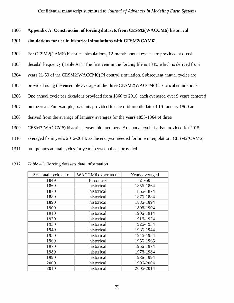
Confidential manuscript submitted to Journal of Advances in Modeling Earth Systems
73
Appendix A: Construction of forcing datasets from CESM2(WACCM6) historical 1300
simulations for use in historical simulations with CESM2(CAM6) 1301
For CESM2(CAM6) historical simulations, 12-month annual cycles are provided at quasi-1302
decadal frequency (Table A1). The first year in the forcing file is 1849, which is derived from 1303
years 21-50 of the CESM2(WACCM6) PI control simulation. Subsequent annual cycles are 1304
provided using the ensemble average of the three CESM2(WACCM6) historical simulations. 1305
One annual cycle per decade is provided from 1860 to 2010, each averaged over 9 years centered 1306
on the year. For example, oxidants provided for the mid-month date of 16 January 1860 are 1307
derived from the average of January averages for the years 1856-1864 of three 1308
CESM2(WACCM6) historical ensemble members. An annual cycle is also provided for 2015, 1309
averaged from years 2012-2014, as the end year needed for time interpolation. CESM2(CAM6) 1310
interpolates annual cycles for years between those provided. 1311
Table A1. Forcing datasets date information 1312
Seasonal cycle date WACCM6 experiment Years averaged
1849 PI control 21-50
1860 historical 1856-1864
1870 historical 1866-1874
1880 historical 1876-1884
1890 historical 1886-1894
1900 historical 1896-1904
1910 historical 1906-1914
1920 historical 1916-1924
1930 historical 1926-1934
1940 historical 1936-1944
1950 historical 1946-1954
1960 historical 1956-1965
1970 historical 1966-1974
1980 historical 1976-1984
1990 historical 1986-1994
2000 historical 1996-2004
2010 historical 2006-2014

Confidential manuscript submitted to Journal of Advances in Modeling Earth Systems
74
2013 historical 2012-2014
2015 historical 2012-2014
References 1313
Ali, A. A., C. Xu, A. Rogers, R. A. Fisher, S. D. Wullschleger, E. C. Massoud, J. A. Vrugt, J. D. 1314
Muss, N. G. McDowell, J. B. Fisher, P. B. Reich, and C. J. Wilson (2016), A global scale 1315
mechanistic model of photosynthetic capacity (LUNA V1.0), Geoscientific Model 1316
Development, 9, 587-606, doi: 10.5194/gmd-9-587-2016. 1317
Armstrong, R. A., C. Lee, J. I. Hedges, S. Honjo, and S. G. Wakeham (2002), A new, 1318
mechanistic model for organic carbon fluxes in the ocean based on the quantitative 1319
association of POC with ballast minerals, Deep-Sea Research, 49, 219-236, doi: 1320
10.1016/S0967-0645(01)00101-1. 1321
Aschwanden, A., M. A. Fahnestock, and M. Truffer (2016), Complex Greenland outlet glacier 1322
flow captured, Nat. Commun., 7, 10524, doi: 10.1038/ncomms10524. 1323
Asselin, R. (1972), Frequency filter for time integrations, Mon. Wea. Rev., 100, 487-490. 1324
Assur, A. (1958), Composition of sea ice and its tensile strength. In Arctic sea ice; Conference 1325
held at Easton, Maryland, February 24–27, 1958, v. 598 of Publs. Natl. Res. Coun. 1326
Wash., pages 106-138, Washington, DC, US. 1327
Beljaars, A. C. M., A. R. Brown, and N. Wood (2004), A new parameterization of turbulent 1328
orographic form drag, Q. J. Roy. Meteor. Soc., 130, 1327-1347, doi: 10.1256/qj.03.73. 1329
Berrisford, P., D. P. K. F. Dee, K. Fielding, M. Fuentes, P. Kallberg, S. Kobayashi, and S. 1330
Uppala (2009), The ERA-interim archive. ERA report series, (1), 1-16, Reading, U. K. 1331
Confidential manuscript submitted to Journal of Advances in Modeling Earth Systems
75
Beusen, A. H. W., L. P. H. Van Beek, A. F. Bouwman, J. M. Mogollón, and J. J. Middelburg 1332
(2015), Coupling global models for hydrology and nutrient loading to simulate nitrogen 1333
and phosphorus retention in surface water – description of IMAGE-GNM and analysis of 1334
performance, Geosci. Model Dev., 8, 4045-4067, doi: 10.5194/gmd-8-4045-2015. 1335
Beusen, A. H. W., A. F. Bouwman, L. P. H. Van Beek, J. M. Mogollón, and J. J. Middelburg 1336
(2016), Global riverine N and P transport to ocean increased during the 20th century 1337
despite increased retention along the aquatic continuum, Biogeosciences, 13, 2441-2451, 1338
doi: 10.5194/bg-13-2441-2016. 1339
Bogenschutz, P. A., A. Gettelman, H. Morrison, V. E. Larson, C. Craig, and D. P. Schanen 1340
(2013), Higher-order turbulence closure and its impact on climate simulation in the 1341
Community Atmosphere Model, J. Climate, 26, 9655-9676, doi: 10.1175/JCLI-D-13-1342
00075.1. 1343
Bonan, G. B., P. J. Lawrence, K. W. Oleson, S. Levis, M. Jung, M. Reichstein, D. M. Lawrence, 1344
and S. C. Swenson (2011), Improving canopy processes in the Community Land Model 1345
version 4 (CLM4) using global flux fields empirically inferred from FLUXNET data, J. 1346
Geophys. Res. Biogeosciences, 116(G2), doi: 10.1029/2010jg001593. 1347
Bonan, G. B., D. L. Lombardozzi, W. R. Wieder, K. W. Oleson, D. M. Lawrence, F. M. 1348
Hoffman, and N. Collier (2019), Model structure and climate data uncertainty in 1349
historical simulations of the terrestrial carbon cycle (1850-2014), Global Biogeochemical 1350
Cycles, doi: 10.1029/2019GB006175. 1351
Boville, B. A., and P. R. Gent (1998), The NCAR Climate System Model, version one, J. 1352
Climate, 11, 1115-1130. 1353
Confidential manuscript submitted to Journal of Advances in Modeling Earth Systems
76
Brunke, M. A., P. Broxton, J. Pelletier, D. Gochis, P. Hazenberg, D. M. Lawrence, L. R. Leung, 1354
G.-Y. Niu, P. A. Troch, and X. Zeng (2016), Implementing and evaluating variable soil 1355
thickness in the Community Land Model, version 4.5 (CLM4.5), J. Climate, 29, 3441-1356
3461, doi: 10.1175/JCLI-D-15-0307.1. 1357
Cavaleri, L., B. Fox-Kemper, and M. Hemer (2012), Wind waves in the coupled climate system, 1358
Bull. Amer. Meteor. Soc., 93, 1651-1661. 1359
Cavalieri, D. J., C. L. Parkinson, P. Gloersen, and H. J. Zwally (1996), updated yearly. Sea ice 1360
concentrations from Nimbus-7 SMMR and DMSP SSM/I-SSMIS passive microwave 1361
data, version 1. Boulder, Colorado USA. NASA National Snow and Ice Data Center 1362
Distributed Active Archive Center. doi: 10.5067/8GQ8LZQVL0VL. 1363
Collier, N., F. M. Hoffman, D. M. Lawrence, G. Keppel-Aleks, C. D. Koven, W. J. Riley, M. 1364
Mu, and J. T. Randerson (2018), The International Land 1 Model Benchmarking 1365
(ILAMB) system: Design, theory, and implementation. J. Advances in Modeling Earth 1366
Systems, doi: 10.1029/2018MS001354. 1367
Collins, W. D., C. M. Bitz, M. L. Blackmon, G. B. Bonan, C. S. Bretherton, J. A. Carton, P. 1368
Chang, S. C. Doney, J. J. Hack, T. B. Henderson, J. T. Kiehl, W. G. Large, D. D. 1369
McKenna, B. D. Santer, and R. D. Smith (2006), The Community Climate System Model 1370
version 3 (CCSM3), J. Climate, 19, 2122-2143. 1371
Danabasoglu, G., and P. R. Gent (2009), Equilibrium climate sensitivity: Is it accurate to use a 1372
slab ocean model? J. Climate, 22, 2494-2499, doi: 10.1175/2008JCLI2596.1. 1373
Danabasoglu, G., W. G. Large, and B. P. Briegleb (2010), Climate impacts of parameterized 1374
Nordic Sea overflows, J. Geophys. Res., 115, C11005, doi:10.1029/2010JC006243. 1375
Confidential manuscript submitted to Journal of Advances in Modeling Earth Systems
77
Danabasoglu, G., S. C. Bates, B. P. Briegleb, S. R. Jayne, M. Jochum, W. G. Large, S. Peacock, 1376
and S. G. Yeager (2012), The CCSM4 ocean component, J. Climate, 25, 1361-1389, doi: 1377
10.1175/JCLI-D-11-00091.1. 1378
Dee, D. P., S. M. Uppala, A. J. Simmons, P. Berrisford, P. Poli, S. Kobayashi, U. Andrae, 1379
M. A. Balmaseda, G. Balsamo, P. Bauer, P. Bechtold, A. C. M. Beljaars, L. van de 1380
Berg, J. Bidlot, N. Bormann, C. Delsol, R. Dragani, M. Fuentes, A. J. Geer, L. 1381
Haimberger, S. B. Healy, H. Hersbach, E. V. Holm, L. Isaksen, P. Kallberg, M. 1382
Kohler, M. Matricardi, A. P. McNally, B. M. Monge-Sanz, J.-J. Morcrette, B.-K. 1383
Park, C. Peubey, P. de Rosnay, C. Tavolato, J.-N. Thepaut, and F. Vitart (2011), 1384
The ERA-Interim reanalysis: Configuration and performance of the data 1385
assimilation system, Q. J. R. Meteorol. Soc., 137, 553-597. 1386
Deser, C., A. S. Phillips, R. A. Tomas, Y. Okumura, M. A. Alexander, A. Capotondi, J. D. Scott, 1387
Y.-O. Kwon, and M. Ohba (2012), ENSO and Pacific decadal variability in Community 1388
Climate System Model version 4, J. Climate, 25, 2622-2651, doi: 10.1175/JCLI-D-11-1389
00301.1. 1390
Deser, C., R. Guo, and F. Lehner (2017), The relative contributions of tropical Pacific sea 1391
surface temperatures and atmospheric internal variability to the recent global warming 1392
hiatus, Geophys. Res. Lett., 44, doi: 10.1002/2017GL074273. 1393
Eyring, V., S. Bony, G. A. Meehl, C. A. Senior, B. Stevens, R. J. Stouffer, and K. E. Taylor 1394
(2016), Overview of the Coupled Model Intercomparison Project phase 6 (CMIP6) 1395
experimental design and organization, Geosci. Model Dev., 9, 1937-1958, doi: 1396
10.5194/gmd-9-1937-2016. 1397
Confidential manuscript submitted to Journal of Advances in Modeling Earth Systems
78
Eyring, V., L. Bock, A. Lauer, M. Righi, M. Schlund, B. Andela, E. Arnone, O. Bellprat, B. 1398
Brötz, L.-P. Caron, N. Carvalhais, I. Cionni, N. Cortesi, B. Crezee, E. Davin, P. Davini, 1399
K. Debeire, L. de Mora, C. Deser, D. Docquier, P. Earnshaw, C. Ehbrecht, B. K. Gier, N. 1400
Gonzalez-Reviriego, P. Goodman, S. Hagemann, S. Hardiman, B. Hassler, A. Hunter, C. 1401
Kadow, S. Kindermann, S. Koirala, N. V. Koldunov, Q. Lejeune, V. Lembo, T. Lovato, 1402
V. Lucarini, F. Massonnet, B. Müller, A. Pandde, N. Pérez-Zanón, A. Phillips, V. Predoi, 1403
J. Russell, A. Sellar, F. Serva, T. Stacke, R. Swaminathan, V. Torralba, J. Vegas-Regidor, 1404
J. von Hardenberg, K. Weigel, and K. Zimmermann (2020), ESMValTool v2.0 – 1405
Extended set of large-scale diagnostics for quasi-operational and comprehensive 1406
evaluation of Earth system models in CMIP, Geosci. Model Dev. Discuss., doi: 1407
10.5194/gmd-2019-291 (in review). 1408
Fisher, R. A., W. R. Wieder, B. M. Sanderson, C. D. Koven, K. W. Oleson, C. Xu, J. B. Fisher, 1409
M. Shi, A. P. Walker, and D. M. Lawrence (2019), Parametric controls on vegetation 1410
responses to biogeochemical forcing in the CLM5, J. Advances in Modeling Earth 1411
Systems, 11, doi: 10.1029/2019MS001609. 1412
Frajka-Williams, E., S. A. Cunningham, H. Bryden, and B. A. King (2011), Variability of 1413
Antarctic Bottom Water at 24.5°N in the Atlantic, J. Geophys. Res., 116, C11026, doi: 1414
10.1029/2011JC007168. 1415
Frajka-Williams, E., I. J. Ansorge, J. Baehr, H. L. Bryden, M. Paz Chidichimo, S. A. 1416
Cunningham, G. Danabasoglu, S. Dong, K. A. Donohue, S. Elipot, P. Heimbach, N. P. 1417
Holliday, R. Hummels, L. C. Jackson, J. Karstensen, M. Lankhorst, I. A. Le Bras, M. S. 1418
Lozier, E. L. McDonagh, C. S. Meinen, H. Mercier, B. I. Moat, R. C. Perez, C. G. 1419
Piecuch, M. Rhein, M. A. Srokosz, K. E. Trenberth, S. Bacon, G. Forget, G. Goni, D. 1420
Confidential manuscript submitted to Journal of Advances in Modeling Earth Systems
79
Kieke, J. Koelling, T. Lamont, G. D. McCarthy, C. Mertens, U. Send, D. A. Smeed, S. 1421
Speich, M. van den Berg, D. Volkov, and C. Wilson (2019), Atlantic meridional 1422
overturning circulation: Observed transport and variability, Front. Mar. Sci., 6:260, doi: 1423
10.3389/fmars.2019.00260. 1424
Galbraith, E. D., and A. C. Martiny (2015), A simple nutrient-dependence mechanism for 1425
predicting the stoichiometry of marine ecosystems, Proceedings of the National Academy 1426
of Sciences of the United States of America, 112, 8199-8204, doi: 1427
10.1073/pnas.1423917112. 1428
Gent, P. R., G. Danabasoglu, L. J. Donner, M. M. Holland, E. C. Hunke, S. R. Jayne, D. M. 1429
Lawrence, R. B. Neale, P. J. Rasch, M. Vertenstein, P. H. Worley, Z.-L. Yang, and M. 1430
Zhang (2011), The Community Climate System Model version 4, J. Climate, 24, 4973-1431
4991, doi: 10.1175/2011JCLI4083.1. 1432
Gettelman, A., J. E. Kay, and K. M. Shell (2012), The evolution of climate sensitivity and 1433
climate feedbacks in the Community Atmosphere Model, J. Climate, 25, 1453-1469, doi: 1434
10.1175/JCLI-D-11-00197.1. 1435
Gettelman, A., and H. Morrison (2015), Advanced two-moment bulk microphysics for global 1436
models. Part I: Off-line tests and comparison with other schemes, J. Climate, 28, 1268-1437
1287, doi: 10.1175/JCLI-D-14-00102.1. 1438
Gettelman, A., M. J. Mills, D. E. Kinnison, R. R. Garcia, A. K. Smith, D. R. Marsh, S. Tilmes, F. 1439
Vitt, C. G. Bardeen, J. McInerny, H.-L. Liu, S. C. Solomon, L. M. Polvani, L. K. 1440
Emmons, J.-F. Lamarque, J. H. Richter, A. S. Glanville, J. T. Bacmeister, A. S. Philips, 1441
R. B. Neale, I. R. Simpson, A. K. DuVivier, A. Hodzic, and W. J. Randel (2019a), The 1442
Confidential manuscript submitted to Journal of Advances in Modeling Earth Systems
80
Whole Atmosphere Community Climate Model version 6 (WACCM6), J. Geophys. Res. 1443
Atmos., 124, doi: 10.1029/2019JD030943. 1444
Gettelman, A., C. Hannay, and J. T. Bacmesiter, R. B. Neale, A. G. Pendergrass, G. 1445
Danabasoglu, J.-F. Lamarque, J. T. Fasullo, D. A. Bailey, and D. M. Lawrence (2019b), 1446
High climate sensitivity in the Community Earth System Model version 2 (CESM2), 1447
Geophys. Res. Lett., 46, 8329-8337, doi: 10.1029/2019GL083978. 1448
Ghimire, B., W. J. Riley, C. D. Koven, M. Q. Mu, and J. T. Randerson (2016), Representing leaf 1449
and root physiological traits in CLM improves global carbon and nitrogen cycling 1450
predictions, J. of Advances in Modeling Earth Systems, 8, 598-613, doi: 1451
10.1002/2015MS000538. 1452
Goldberg, D. N. (2011), A variationally derived, depth-integrated approximation to a higher-1453
order glaciological flow model, J. Glaciol., 57, 157-170, doi: 1454
10.3189/002214311795306763. 1455
Golaz, J.-C., V. E. Larson, and W. R. Cotton (2002), A PDF-based model for boundary layer 1456
clouds. Part I: Method and model description, J. Atmos. Sci., 59, 3540-3551. 1457
Gregory, J. M., W. J. Ingram, M. A. Palmer, G. S. Jones, P. A. Stott, R. B. Thorpe, J. A. Lowe, 1458
T. C. Johns, and K. D. Williams (2004), A new method for diagnosing radiative forcing 1459
and climate sensitivity, Geophys. Res. Lett., 31, L03205, doi: 10.1029/2003GL018747. 1460
Hemer, M. A., X. L. Wang, R. Weisse, and V. R. Swail (2012), Advancing wind-waves climate 1461
science: The COWCLIP project, Bull. Amer. Meteor. Soc., 93, 791-796. 1462
Hoesly, R. M., S. J. Smith, L. Feng, Z. Klimont, G. Janssens-Maenhout, T. Pitkanen, J. J. 1463
Seibert, L. Vu, R. J. Andres, R. M. Bolt, T. C. Bond, L. Dawidowski, N. Kholod, J.-I. 1464
Confidential manuscript submitted to Journal of Advances in Modeling Earth Systems
81
Kurokawa, M. Li, L. Liu, Z. Lu, M. C. P. Moura, P. R. O’Rourke, and Q. Zhang (2018), 1465
Historical (1750-2014) anthropogenic emissions of reactive gases and aerosols from the 1466
Community Emissions Data System (CEDS), Geosci. Model Dev., 11, 369-408, doi: 1467
10.5194/gmd-11-369-2018. 1468
Hoose, C., J. E. Kristjánsson, J.-P. Chen, and A. Hazra (2010), A classical-theory-based 1469
parameterization of heterogeneous ice nucleation by mineral dust, soot, and biological 1470
particles in a global climate model, J. Atmos. Sci., 67, 2483-2503, doi: 1471
10.1175/2010JAS3425.1. 1472
Huang, B., P. W. Thorne, V. F. Banzon, T. Boyer, G. Chepurin, J. H. Lawrimore, M. J. Menne, 1473
T. M. Smith, R. S. Vose, and H.-M. Zhang (2017), Extended Reconstructed Sea Surface 1474
Temperature, version 5 (ERSSTv5): Upgrades, validations, and intercomparisons, J. 1475
Climate, 30, 8179-8205, doi: 10.1175/JCLI-D-16-0836.1. 1476
Huang, X., Q. Tang, Y. Tseng, Y. Hu, A. H. Baker, F. O. Bryan, J. Dennis, H. Fu, and G. Yang 1477
(2016), P-CSI v1.0, An accelerated barotropic solver for the high-resolution ocean model 1478
component in the Community Earth System Model v2.0, Geosci. Model Dev., 9, 4209-1479
4225, doi: 10.5194/gmd-9-4209-2016. 1480
Huffman, G. J., R. F. Adler, D. T Bolvin, and G. Gu (2009), Improving the global precipitation 1481
record: GPCP Version 2.1, Geophys. Res. Lett., 36, L17808, doi: 1482
10.1029/2009GL040000. 1483
Hunke, E. C., D. A. Hebert, and O. Lecomte (2013), Level-ice melt ponds in the Los Alamos sea 1484
ice model, CICE, Ocean Modell., 71, 26-42, doi: 10.1016/j.ocemod.2012.11.008. 1485
Confidential manuscript submitted to Journal of Advances in Modeling Earth Systems
82
Hunke, E. C, W. H. Lipscomb, A. K. Turner, N. Jeffery, and S. Elliott (2015), CICE: The Los 1486
Alamos Sea Ice Model. Documentation and Software User’s Manual. Version 5.1. T-3 1487
Fluid Dynamics Group, Los Alamos National Laboratory, Tech. Rep. LA-CC-06-012. 1488
Hurrell, J. W., M. M. Holland, P. R. Gent, S. Ghan, J. E. Kay, P. J. Kushner, J.-F. Lamarque, W. 1489
G. Large, D. Lawrence, K. Lindsay, W. H. Lipscomb, M. C. Long, N. Mahowald, D. R. 1490
Marsh, R. B. Neale, P. Rasch, S. Vavrus, M. Vertenstein, D. Bader, W. D. Collins, J. J. 1491
Hack, J. Kiehl, and S. Marshall (2013), The Community Earth System Model: A 1492
framework for collaborative research, Bull. Amer. Meteor. Soc., 94, 1339-1360, doi: 1493
10.1175/BAMS-D-12-00121.1. 1494
Iacono, M. J., J. S. Delamere, E. J. Mlawer, M. W. Shephard, S. A. Clough, and W. D. Collins 1495
(2008), Radiative forcing by long-lived greenhouse gases: Calculations with the AER 1496
radiative transfer models, J. Geophys. Res., 113, D13103, doi: 10.1029/2008JD009944. 1497
Jones, P. D., D. H. Lister, T. J. Osborn, C. Harpham, M. Salmon, and C. P. Morice (2012), 1498
Hemispheric and large-scale land surface air temperature variations: An extensive 1499
revision and an update to 2010, J. Geophys. Res., 117, D05127, doi: 1500
10.1029/2011JD017139. 1501
Kaufmann, R. K., H. Kauppi, M. L. Mann, and J. H. Stock (2011), Reconciling anthropogenic 1502
climate change with observed temperature 1998-2008, Proc. Nat. Academy Sci., 108, 1503
11790-11793, doi: 10.1073/pnas.1102467108. 1504
Kay, J. E., C. Deser, A. Phillips, A. Mai, C. Hannay, G. Strand, J. Arblaster, S. Bates, G. 1505
Danabasoglu, J. Edwards, M. Holland, P. Kushner, J.-F. Lamarque, D. Lawrence, K. 1506
Lindsay, A. Middleton, E. Munoz, R. Neale, K. Oleson, L. Polvani, and M. Vertenstein 1507

Confidential manuscript submitted to Journal of Advances in Modeling Earth Systems
83
(2015), The Community Earth System Model (CESM) Large Ensemble project: A 1508
community resource for studying climate change in the presence of internal climate 1509
variability, Bull. Amer. Meteor. Soc., 96, 1333-1349, doi:10.1175/BAMS-D-13-00255.1. 1510
Kennedy, D., S. Swenson, K. W. Oleson, D. M. Lawrence, R. Fisher, A. C. L. da Costa, and P. 1511
Gentine (2019), Implementing plant hydraulics in the Community Land Model, version 5, 1512
J. Advances in Modeling Earth Systems, 11, 485-513, doi: 10.1029/2018ms001500. 1513
Kiehl, J. T., and P. R. Gent (2004), The Community Climate System Model, version 2. J. 1514
Climate, 17, 3666–3682. 1515
Knutti, R., D. Masson, and A. Gettelman (2013), Climate model genealogy: Generation CMIP5 1516
and how we got there, Geophys. Res. Lett., 40, 1194-1199, doi: 10.1002/grl.50256. 1517
Kosaka, Y., and S.-P. Xie (2013), Recent global-warming hiatus tied to equatorial Pacific surface 1518
cooling, Nature, 501, 403-407, doi: 10.1038/nature12534. 1519
Koven, C. D., W. J. Riley, Z. M. Subin, J. Y. Tang, M. S. Torn, W. D. Collins, G. B. Bonan, D. 1520
M. Lawrence, and S. C. Swenson (2013), The effect of vertically resolved soil 1521
biogeochemistry and alternate soil C and N models on C dynamics of CLM4, 1522
Biogeosciences, 10, 7109-7131, doi: 10.5194/bg-10-7109-2013. 1523
Kummerow, C., J. Simpson, O. Thiele, W. Barnes, A. T. Chang, E. Stocker, R. F. Adler, A. Hou, 1524
R. Kakar, F. Wentz, P. Ashcroft, T. Kozu, Y. Hong, K. Okamoto, T. Iguchi, H. Kuroiwa, 1525
E. Im, Z. Haddad, G. Huffman, B. Ferrier, W. S. Olson, E. Zipser, E.A. Smith, T. T. 1526
Wilheit, G. North, T. Krishnamurti, and K. Nakamura (2000), The status of the Tropical 1527
Rainfall Measuring Mission (TRMM) after two years in orbit, J. Appl. Meteor., 39, 1965-1528
1982, doi: 10.1175/1520-0450(2001)040<1965:TSOTTR>2.0.CO;2. 1529
Confidential manuscript submitted to Journal of Advances in Modeling Earth Systems
84
Large, W. G., J. C. McWilliams, and S. C. Doney (1994), Oceanic vertical mixing: A review and 1530
a model with a nonlocal boundary layer parameterization, Rev. Geophys., 32, 363-403. 1531
Larson, V. E., (2017), CLUBB-SILHS: A parameterization of subgrid variability in the 1532
atmosphere. arXiv:1711.03675v2 [physics.ao-ph]. 1533
Lawrence, D. M., R. A. Fisher, C. D. Koven, K. W. Oleson, S. C. Swenson, G. Bonan, N. 1534
Collier, B. Ghimire, L. van Kampenhout, D. Kennedy, E. Kluzek, P. J. Lawrence, F. Li, 1535
H. Li, D. Lombardozzi, W. J. Riley, W. J. Sacks, M. Shi, M. Vertenstein, W. R. Wieder,, 1536
C. Xu, A. A. Ali, A. M. Badger, G. Bisht, M. A. Brunke, S. P. Burns, J. Buzan, M. Clark, 1537
A. Craig, K. Dahlin, B. Drewniak, J. B. Fisher, M. Flanner, A. M. Fox, P. Gentine, F. 1538
Hoffman, G. Keppel-Aleks, R., Knox, S. Kumar, J. Lenaerts, L. R. Leung, W. H. 1539
Lipscomb, Y. Lu, A., Pandey, J. D. Pelletier, J. Perket,, J. T. Randerson, D. M. Ricciuto, 1540
B. M., Sanderson, A. Slater, Z. M. Subin, J. Tang, R. Q. Thomas, M. Val Martin, and X. 1541
Zeng (2019), The Community Land Model version 5: Description of new features, 1542
benchmarking, and impact of forcing uncertainty, J. Advances in Modeling Earth 1543
Systems, 11, doi: 10.1029/2018MS001583. 1544
Lehner, B., K. Verdin, and A. Jarvis (2008), New global hydrography derived from spaceborne 1545
elevation data, AGU Eos Trans., 89, 93-94. 1546
Le Quéré, C., R. M. Andrew, J. G. Canadell, S. Sitch, J. I. Korsbakken, G. P. Peters, A. C. 1547
Manning, T. A. Boden, P. P. Tans, R. A. Houghton, R. F. Keeling, S. Alin, O. 1548
D. Andrews, P. Anthoni, L. Barbero, L. Bopp, F. Chevallier, L. P. Chini, P. Ciais, K. 1549
Currie, C. Delire, S. C. Doney, P. Friedlingstein, T. Gkritzalis, I. Harris, J. Hauck, V. 1550
Haverd, M. Hoppema, K. Goldewijk, A. K. Jain, E. Kato, A. Körtzinger, P. 1551
Landschützer, N. Lefèvre, A. Lenton, S. Lienert, D. Lombardozzi, J. R. Melton, N. 1552
Confidential manuscript submitted to Journal of Advances in Modeling Earth Systems
85
Metzl, F. Millero, P. M. S. Monteiro, D. R. Munro, J. E. M. S. Nabel, S. Nakaoka, K. 1553
O’Brien, A. Olsen, A. M. Omar, T. Ono, D. Pierrot, B. Poulter, C. Rödenbeck, J. 1554
Salisbury, U. Schuster, J. Schwinger, R. Séférian, I. Skjelvan, B. D. Stocker, A. J. Sutton, 1555
T. Takahashi, H. Tian, B. Tilbrook, I. T. van der Laan-Luijkx, G. R. van der Werf, N. 1556
Viovy, A. P. Walker, A. J. Wiltshire, and S. Zaehle (2016), Global Carbon Budget 2016, 1557
Earth Syst. Sci. Data, 8, 605-649, doi:10.5194/essd-8-605-2016. 1558
Lenssen, N., G. Schmidt, J. Hansen, M. Menne, A. Persin, R. Ruedy, and D. Zyss (2019), 1559
Improvements in GISTEMP uncertainty model, J. Geophys. Res. Atmos., 124, 6307-1560
6326, doi: 10.1029/2018JD029522. 1561
Letscher, R. T., J. K. Moore, Y. C. Teng, and F. Primeau (2015), Variable C:N:P stoichiometry 1562
of dissolved organic matter cycling in the Community Earth System Model, 1563
Biogeosciences, 12, 209-221, doi: 10.5194/bg-12-209-2015. 1564
Levis, S., A. Badger, B. Drewniak, C. Nevison, and X. L. Ren (2018), CLMcrop yields and 1565
water requirements: Avoided impacts by choosing RCP 4.5 over 8.5, Climatic Change, 1566
146, 501-515 doi: 10.1007/s10584-016-1654-9. 1567
Levitus, S., T. Boyer, M. Concright, D. Johnson, T. O’Brien, J. Antonov, C. Stephens, and R. 1568
Garfield (1998), Introduction, Vol. I, World Ocean Database 1998, NOAA Atlas 1569
NESDIS 18, 346 pp. 1570
Li, F., S. Levis, S., and D. S. Ward (2013), Quantifying the role of fire in the Earth system - Part 1571
1: Improved global fire modeling in the Community Earth System Model (CESM1), 1572
Biogeosciences, 10, 2293-2314, doi: 10.5194/bg-10-2293-2013. 1573
Confidential manuscript submitted to Journal of Advances in Modeling Earth Systems
86
Li, F., and D. M. Lawrence (2017), Role of fire in the global land water budget during the 1574
twentieth century due to changing ecosystems, J. Climate, 30, 1893-1908, doi: 1575
10.1175/JCLI-D-16-0460.1. 1576
Li, H. Y., M. S. Wigmosta, H. Wu, M. Y. Huang, Y. H. Ke, A. M. Coleman, and L. R. Leung 1577
(2013), A physically based runoff routing model for land surface and Earth system 1578
models, J. Hydrometeorology, 14, 808-828, doi: 10.1175/Jhm-D-12-015.1. 1579
Li, Q., A. Webb, B. Fox-Kemper, A. Craig, G. Danabasoglu, W. G. Large, and M. Vertenstein 1580
(2016), Langmuir mixing effects on global climate: WAVEWATCH III in CESM, Ocean 1581
Modell., 103, 145-160, doi: 10.1016/j.ocemod.2015.07.020. 1582
Li, Q., B. Fox-Kemper, O. Breivik, and A. Webb (2017), Statistical models of global Langmuir 1583
mixing, Ocean Modell., 113, 95-114. 1584
Li, Q., and B. Fox-Kemper (2017), Assessing the effects of Langmuir turbulence on the 1585
entrainment buoyancy flux in the ocean surface boundary layer, J. Phys. Oceanogr., 47, 1586
2863-2886. 1587
Lin, S. J., and R. B. Rood (1997), An explicit Flux-Form Semi-Lagrangian shallow water model 1588
on the sphere, Q. J. Royal Meteor. Soc., 123, 2477-2498. 1589
Lindsay, K. (2017), A Newton-Krylov solver for fast spin-up of online ocean tracers, Ocean 1590
Modell., 109, 33-43, doi: 10.1016/j.ocemod.2016.12.001. 1591
Lipscomb, W. H., J. G. Fyke, M. Vizcaíno, W. J. Sacks, J. Wolfe, M. Vertenstein, A. Craig, E. 1592
Kluzek, and D. M. Lawrence (2013), Implementation and initial evaluation of the 1593
Glimmer Community Ice Sheet Model in the Community Earth System Model, J. 1594
Climate, 26, 7352-7371, doi: 10.1175/JCLI-D-12-00557.1. 1595
Confidential manuscript submitted to Journal of Advances in Modeling Earth Systems
87
Lipscomb, W. H., S. F. Price, M. J. Hoffman, G. R. Leguy, A. R. Bennett, S. L. Bradley, K. J. 1596
Evans, J. G. Fyke, J. H. Kennedy, M. Perego, D. M. Ranken, W. J. Sacks, A. G. Salinger, 1597
L. Vargo, and P. H. Worley (2019), Description and evaluation of the Community Ice 1598
Sheet Model (CISM) v. 2.1, Geosci. Model Dev., 12, 387-424, doi: 10.5194/gmd-12-387-1599
2019. 1600
Liu, X., P. L. Ma, H. Wang, S. Tilmes, B. Singh, R. C. Easter, S. J. Ghan, and P. J. Rasch (2016), 1601
Description and evaluation of a new four-mode version of the Modal Aerosol Module 1602
(MAM4) within version 5.3 of the Community Atmosphere Model, Geosci. Model Dev., 1603
9, 505-522, doi: 10.5194/gmd-9-505-2016. 1604
Loeb, N. A., B. A. Wielicki, D. R. Doelling, G. L. Smith, D. F. Keyes, S. Kato, N. Manalo-1605
Smith, and T. Wong (2009), Toward optimal closure of the Earth's top-of-atmosphere 1606
radiation budget, J. Climate, 22, 748-766. 1607
Lombardozzi, D. L., G. B. Bonan, N. G. Smith, J. S. Dukes, and R. A. Fisher (2015), 1608
Temperature acclimation of photosynthesis and respiration: A key uncertainty in the 1609
carbon cycle‐climate feedback. Geophys. Res. Lett., 42, 8624-8631. 1610
Long, M. C., K. Lindsay, and M. M. Holland (2015), Modeling photosynthesis in sea ice covered 1611
waters, J. Advances in Modeling Earth Systems, 7, 1189-1206, doi: 1612
10.1002/2015MS000436. 1613
Malavelle, F. F., J. M. Haywood, A. Jones, A. Gettelman, L. Clarisse, S. Bauduin, R. P. Allan, I. 1614
H. H. Karset, J. E. Kristjansson, L. Oreopoulos, N. Cho, D. Lee, N. Bellouin, O. Boucher, 1615
D. P. Grosvenor, K. S. Carslaw, S. Dhomse, G. W. Mann, A. Schmidt, H. Coe, M. E. 1616
Hartley, M. Dalvi, A. A. Hill, B. T. Johnson, C. E. Johnson, J. R. Knight, F. M. 1617
Confidential manuscript submitted to Journal of Advances in Modeling Earth Systems
88
O’Connor, D. G. Partridge, P. Stier, G. Myhre, S. Platnick, G. L. Stephens, H. Takahashi, 1618
and T. Thordarson (2017), Strong constraints on aerosol – cloud interactions from 1619
volcanic eruptions, Nature, 546, 485-491, doi: 10.1038/nature22974. 1620
Mayorga, E., S. P. Seitzinger, J. A., Harrison, E. Dumont, A. H. W. Beusen, A. F. Bouwman, B. 1621
M. Fekete, C. Kroeze, and G. van Drecht (2010), Global Nutrient Export from 1622
WaterSheds 2 (NEWS 2): Model development and implementation, Environmental 1623
Modelling and Software[R], 25, 837-853, doi: 10.1016/j.envsoft.2010.01.007. 1624
McWilliams, J. C., and B. Fox-Kemper (2013), Oceanic wave-balanced surface fronts and 1625
filaments, J. Fluid Mech., 730, 464-490, doi: 10.1017/jfm.2013.348. 1626
McWilliams, J. C., and P. Sullivan (2000), Vertical mixing by Langmuir circulations, Spill 1627
Science and Technology Bull., 6, 225-237. 1628
Meehl, G. A., W. M. Washington, J. M. Arblaster, A. Hu, H. Teng, J. E. Kay, A. Gettelman, D. 1629
M. Lawrence, B. M. Sanderson, and W. G. Strand (2013), Climate change projections in 1630
CESM1(CAM5) compared to CESM4, J. Climate, 26, 6287-6308, doi: 10.1175/JCLI-D-1631
12-00572.1. 1632
Meehl, G. A., H. Teng, and J. M. Arblaster (2014), Climate model simulations of the observed 1633
early-2000s hiatus of global warming, Nature Climate Change, 4, 898-902, doi: 1634
10.1038/NCLIMATE2357. 1635
Meinshausen, M., E. Vogel, A. Nauels, K. Lorbacher, N. Meinshausen, D. M. Etheridge, P. J. 1636
Fraser, S. A. Montzka, P. J. Rayner, C. M. Trudinger, P. B. Krummel, U. Beyerle, J. G. 1637
Canadell, J. S. Daniel, I. G. Enting, R. M. Law, C. R. Lunder, S. O'Doherty, R. G. Prinn, 1638
S. Reimann, M. Rubino, G. J. M. Velders, M. K. Vollmer, R. H. J. Wang, and R. Weiss 1639

Confidential manuscript submitted to Journal of Advances in Modeling Earth Systems
89
(2017), Historical greenhouse concentrations for climate modelling (CMIP6), Geosci. 1640
Model Dev., 10, 2057-2116, doi: 10.5194/gmd-10-2057-2017. 1641
Mills, M. J., A. Schmidt, R. Easter, S. Solomon, D. E. Kinnison, S. J. Ghan, R. R. Neely, D. R. 1642
Marsh, A. Conley, C. G. Bardeen, and A. Gettelman (2016), Global volcanic aerosol 1643
properties derived from emissions, 1990–2014, using CESM1(WACCM), J. Geophys. 1644
Res. Atmos., 121, 2332-2348, doi: 10.1002/2015JD024290. 1645
Mills, M. J., J. H. Richter, S. Tilmes, B. Kravitz, D. G. MacMartin, A. A. Glanville, J. J. Tribbia, 1646
J.-F. Lamarque, F. Vitt, A. Schmidt, A. Gettelman, C. Hannay, J. T. Bacmeister, and D. 1647
E. Kinnison (2017), Radiative and chemical response to interactive stratospheric sulfate 1648
aerosols in fully coupled CESM1(WACCM), J. Geophys. Res. Atmos., 122, doi: 1649
10.1002/2017JD027006. 1650
Montzka, S. A., M. Aydin, M. Battle, J. H. Butler, E. S. Saltzman, B. D. Hall, A. D. Clarke, D. 1651
Mondeel, and J. W. Elkins (2004), A 350-year atmospheric history for carbonyl sulfide 1652
inferred from Antarctic firn air and air trapped in ice, J. Geophys. Res. Atmos., 109, 1653
D22302, doi: 10.1029/2004JD004686. 1654
Moore, J. K., S. C. Doney, J. A. Kleypas, D. M. Glover, and I. Y. Fung (2002), An intermediate 1655
complexity marine ecosystem model for the global domain, Deep Sea Res., 49, 403-462, 1656
doi: 10.1016/S0967-0645(01)00108-4. 1657
Moore, J. K., S. C. Doney, and K. Lindsay (2004), Upper ocean ecosystem dynamics and iron 1658
cycling in a global three-dimensional model, Global Biogeochemical Cycles, 18, 1659
GB4028, doi: 10.1029/2004GB002220. 1660
Confidential manuscript submitted to Journal of Advances in Modeling Earth Systems
90
Moore, J. K., K. Lindsay, S. C. Doney, M. C. Long, and K. Misumi (2013), Marine Ecosystem 1661
Dynamics and Biogeochemical Cycling in the Community Earth System Model 1662
[CESM1(BGC)]: Comparison of the 1990s with the 2090s under the RCP4.5 and RCP8.5 1663
scenarios, J. Climate, 26, 9291-9312, doi: 10.1175/JCLI-D-12-00566.1. 1664
Morrison, H., and A. Gettelman (2008), A new two-moment bulk stratiform cloud microphysics 1665
scheme in the NCAR community atmosphere model (CAM3), Part I: Description and 1666
numerical tests, J. Climate, 21, 3642-3659. 1667
Neale, R. B., J. H. Richter, and M. Jochum (2008), The impact of convection on ENSO: From a 1668
delayed oscillator to a series of events, J. Climate, 21, 5904-5924. 1669
Neely III, R. R., and A. Schmidt (2016), VolcanEESM: Global volcanic sulphur dioxide (SO2) 1670
emissions database from 1850 to present - Version 1.0. Centre for Environmental Data 1671
Analysis, 04 February 2016, doi: 10.5285/76ebdc0b-0eed-4f70-b89e-55e606bcd568. 1672
Neely III, R. R., D. R. Marsh, K. L. Smith, S. M. Davis, and L. M. Polvani (2014), Biases in 1673
Southern Hemisphere climate trends induced by coarsely specifying the temporal 1674
resolution of stratospheric ozone, Geophys. Res. Lett., 41, 8602-8610, doi: 1675
10.1002/2014GL061627. 1676
Nicolet, M. (1970), Ozone and hydrogen reactions, Annales de Géophysique, 26, 531-546. 1677
Noël, B., W. J. van de Berg, J. M. van Wessem, E. van Meijgaard, D. van As, J. T. M. Lenaerts, 1678
S. Lhermitte, P. Kuipers Munneke, C. J. P. P. Smeets, L. H. van Ulft, R. S. W. van de 1679
Wal, and M. R. van den Broeke (2018), Modelling the climate and surface mass balance 1680
of polar ice sheets using RACMO2 – Part 1: Greenland (1958–2016), The Cryosphere, 1681
12, 811-831, doi: 10.5194/tc-12-811-2018. 1682

Confidential manuscript submitted to Journal of Advances in Modeling Earth Systems
91
Oleson, K. W., and J. Feddema (2019), Parameterization and surface data improvements and 1683
new capabilities for the Community Land Model Urban (CLMU). J. Advances in 1684
Modeling Earth Systems, doi: 10.1029/2018MS001586. 1685
O'Neill, B. C., C. Tebaldi, D. P. van Vuuren, V. Eyring, P. Friedlingstein, G. Hurtt, R. Knutti, E. 1686
Kriegler, J.-F. Lamarque, J. Lowe, G. A. Meehl, R. Moss, K. Riahi, and B. M. Sanderson 1687
(2016), The Scenario Model Intercomparison Project (ScenarioMIP) for CMIP6, Geosci. 1688
Model Dev., 9, 3461-3482. 1689
Otto-Bliesner, B. L., E. C. Brady, and J. Fasullo (2016), Climate variability and change since 850 1690
CE: An ensemble approach with the Community Earth System Model, Bull. Amer. 1691
Meteor. Soc., 97, 735-754, doi: 10.1175/BAMS-D-14-00233.1. 1692
Paulot, F., D. J. Jacob, M. T. Johnson, T. G. Bell, A. R. Baker, W. C. Keene, I. D. Lima, S. C. 1693
Doney, and C. A. Stock (2015), Global oceanic emission of ammonia: Constraints from 1694
seawater and atmospheric observations: Ocean Ammonia Emissions, Global 1695
Biogeochemical Cycles, 29, 1165-1178, doi: 10.1002/2015GB005106. 1696
Poli, P., H. Hersbach, D. P. Dee, P. Berrisford, A. J. Simmons, F. Vitart, P. Laloyaux, D. G. H. 1697
Tan, C. Peubey, J.-N. Thépaut, Y. Trémolet, E. V. Hólm, M. Bonavita, L. Isaksen, and 1698
M. Fisher (2016), ERA-20C: An atmospheric reanalysis of the twentieth century, J. 1699
Climate, 29, 4083-4097, doi: 10.1175/JCLI-D-15-0556.1. 1700
Reichl, B. G., T. Hara, and I. Ginis (2014), Sea state dependence of the wind stress over the 1701
ocean under hurricane winds, J. Geophys. Res. Oceans, 119, 30-51. 1702
Confidential manuscript submitted to Journal of Advances in Modeling Earth Systems
92
Reichl, B. G., and Q. Li (2019), A parameterization with a constrained potential energy 1703
conversion rate of vertical mixing due to Langmuir turbulence, J. Phys. Oceanogr., doi: 1704
10.1175/JPO-D-18-0258.1. 1705
Richter, J. H., and P. J. Rasch (2008), Effects of convective momentum transport on the 1706
atmospheric circulation in the Community Atmosphere Model, version 3, J. Climate, 21, 1707
1487-1499. 1708
Rienecker, M. M., M. J. Suarez, R. Gelaro, R. Todling, J. Bacmeister, E. Liu, M. G. Bosilovich, 1709
S. D. Schubert, L. Takacs, G.-K. Kim, S. Bloom, J. Chen, D. Collins, A. Conalty, A. da 1710
Silva and Coauthors (2011), MERRA: NASA’s Modern-Era Retrospective Analysis for 1711
Research and Applications, J. Climate, 24, 3624-3648, doi: 10.1175/JCLI-D-11-00015.1. 1712
Roach, L. A., C. Horvat, S. M. Dean, and C. M. Bitz, (2018), An emergent sea ice floe size 1713
distribution in a global coupled ocean‐sea ice model, J. Geophys. Res. Oceans, 123, 1714
4322-4337. 1715
Robert, A. J. (1966), The integration of a low order spectral form of the primitive meteorological 1716
equations, J. Meteor. Soc. Japan, 44, 237-245. 1717
Rohde, R., R. Muller, R. Jacobsen, S. Perlmutter, A. Rosenfeld, J. Wurtele, J. Curry, C. 1718
Wickham, and S. Mosher (2013), Berkeley earth temperature averaging process, 1719
Geoinformatics & Geostatistics: An Overview, 1, doi: 10.4172/gigs.1000103. 1720
Schmidt, A., M. J. Mills, S. Ghan, J. M. Gregory, R. P. Allan, T. Andrews, C. G. Bardeen, A. 1721
Conley, P. M. Forster, A. Gettelman, R. W. Portmann, S. Solomon, and O. B. Toon 1722
(2018), Volcanic radiative forcing from 1979 to 2015, J Geophys Res-Atmos., 123, 1723
12491-12508, doi: 10.1029/2018JD028776. 1724
Confidential manuscript submitted to Journal of Advances in Modeling Earth Systems
93
Schweiger, A., R. Lindsay, J. Zhang, M. Steele, and H. Stern (2011), Uncertainty in modeled 1725
Arctic sea ice volume, J. Geophys. Res., doi: 10.1029/2011JC007084. 1726
Scinocca, J., and N. Mcfarlane (2000), The parametrization of drag induced by stratified flow 1727
over anisotropic orography, Q. J. Roy. Meteor. Soc., 126, 2353-2394, doi: 1728
10.1256/smsqj.56801. 1729
Sheng, J.-X., D. K. Weisenstein, B.-P. Luo, E. Rozanov, A. Stenke, J. Anet, H. Bingemer, and T. 1730
Peter (2015), Global atmospheric sulfur budget under volcanically quiescent conditions: 1731
Aerosol-chemistry-climate model predictions and validation, J. Geophys. Res. Atmos., 1732
120, 256-276, doi: 10.1002/2014JD021985. 1733
Shi, M., J. B. Fisher, E. R. Brzostek, and R. P. Phillips (2016), Carbon cost of plant nitrogen 1734
acquisition: Global carbon cycle impact from an improved plant nitrogen cycle in the 1735
Community Land Model, Glob. Chang. Biol., 22, 1299-1314, doi: 10.1111/gcb.13131. 1736
Shi, X., X. Liu, and K. Zhang (2015), Effects of preexisting ice crystals on cirrus clouds and 1737
comparison between different ice nucleation parameterizations with the Community 1738
Atmosphere Model (CAM5), Atmospheric Chemistry and Physics, 15, 1503-1520, doi: 1739
10.5194/acp-15-1503-2015. 1740
Small, R. J., E. Curchitser, K. Hedstrom, B. Kauffman, and W. G. Large (2015), The Benguela 1741
upwelling system: Quantifying the sensitivity to resolution and coastal wind 1742
representation in a global climate model, J. Climate, 28, 9409-9432, doi: 10.1175/JCLI-1743
D-15-0192.1. 1744
Smeed, D. A., S. A. Josey, C. Beaulieu, W. E. Johns, B. I. Moat, E. Frajka-Williams, D. Rayner, 1745
C. S. Meinen, M. O. Baringer, H. L. Bryden, and G. D. McCarthy (2018), The North 1746
Confidential manuscript submitted to Journal of Advances in Modeling Earth Systems
94
Atlantic Ocean is in a state of reduced overturning, Goephys. Res. Lett., 45, 1527-1533, 1747
doi: 10.1002/2017GL076350. 1748
Smith, R., P. Jones, B. Briegleb, F. Bryan, G. Danabasoglu, J. Dennis, J. Dukowicz, C. Eden, B. 1749
Fox-Kemper, P. Gent, M. Hecht, S. Jayne, M. Jochum, W. Large, K. Lindsay, M. 1750
Maltrud, N. Norton, S. Peacock, M. Vertenstein, and S. Yeager (2010), The Parallel 1751
Ocean Program (POP) reference manual, Ocean component of the Community Climate 1752
System Model (CCSM), LANL Tech. Report, LAUR-10-01853, 141 pp. 1753
Solomon, S., K. H. Rosenlof, R. W. Portmann, J. S. Daniel, S. M. Davis, T. J. Sanford, and G.-K. 1754
Plattner (2010), Contributions of stratospheric water vapor to decadal changes in the rate 1755
of global warming, Science, 327, 1219-1223. 1756
Steele, M., R. Morley, and W. Ermold (2001), PHC: A global ocean hydrography with a high 1757
quality Arctic Ocean, J. Climate, 14, 2079-2087. 1758
Stocker, T. F., D. Qin, G. K. Plattner, M. Tignor, S. K. Allen, J. Boschung, A. Nauels, Y. Xia, B. 1759
Bex, and B. M. Midgley (2013), IPCC, 2013: Climate change 2013: The physical science 1760
basis. Contribution of working group I to the fifth assessment report of the 1761
intergovernmental panel on climate change. 1762
Subin, Z. M., W. J. Riley, and D. Mironov (2012), An improved lake model for climate 1763
simulations: Model structure, evaluation, and sensitivity analyses in CESM1. J. of 1764
Advances in Modeling Earth Systems, 4, M02001, doi: 10.1029/2011ms000072. 1765
Sun, Q., M. M. Whitney, F. O. Bryan, and Y.-H. Tseng (2019), Assessing the skill of the 1766
improved treatment of riverine freshwater in the Community Earth System Model 1767
Confidential manuscript submitted to Journal of Advances in Modeling Earth Systems
95
(CESM) relative to a new salinity climatology, J. Advances in Modeling Earth Systems, 1768
11, doi: 10.1029/2018MS001349. 1769
Suzuki, N., and B. Fox-Kemper (2016), Understanding Stokes forces in the wave-averaged 1770
equations, J. Geophys. Res. Oceans, 121, 1-18, doi: 10.1002/2015JC011566. 1771
Swenson, S. C., and D. Lawrence (2012), A new fractional snow‐covered area parameterization 1772
for the Community Land Model and its effect on the surface energy balance. J. Geophys. 1773
Res. Atmos., 117, D21107, doi:10.1029/2012JD018178. 1774
Swenson, S. C., D. M. Lawrence, and H. Lee (2012), Improved simulation of the terrestrial 1775
hydrological cycle in permafrost regions by the Community Land Model. J. of Advances 1776
in Modeling Earth Systems, 4, doi: 10.1029/2012ms000165. 1777
Swenson, S., and D. Lawrence (2014), Assessing a dry surface layer‐based soil resistance 1778
parameterization for the Community Land Model using GRACE and FLUXNET‐MTE 1779
data, J. Geophys. Res. Atmos., 119, 10299-10312, doi: 10.1002/2014JD022314. 1780
Swenson, S., and D. Lawrence (2015), A GRACE‐based assessment of interannual groundwater 1781
dynamics in the Community Land Model, Water Resources Research, 51, 8817-8833. 1782
Thiery, W., A. J. Visser, E. M. Fischer, M. Hauser, A. L. Hirsch, D. M. Lawrence, Q. Lejeune, 1783
E. L. Davin, and S. I. Seneviratne (2020), Warming of hot extremes alleviated by 1784
expanding irrigation, Nature Communications (in press). 1785
Tilmes, S., J. H. Richter, B. Kravitz, D. G. MacMartin, M. J. Mills, I. R. Simpson, A. S. 1786
Glanville, J. T. Fasullo, A. S. Phillips, J.-F. Lamarque, J. Tribbia, J. Edwards, S. 1787
Mickelson, and S. Gosh (2018), CESM1(WACCM) Stratospheric Aerosol 1788
Confidential manuscript submitted to Journal of Advances in Modeling Earth Systems
96
Geoengineering Large Ensemble (GLENS) Project, Bull. Amer. Meteor. Soc., doi: 1789
10.1175/BAMS-D-17-0267.1. 1790
Tilmes, S., A. Hodzic, L. K. Emmons, M. J. Mills, A. Gettelman, D. E. Kinnison, M. Park, J.-F. 1791
Lamarque, F. Vitt, M. Shrivastava, P. Campuzano-Jost, J. Jiminez, and X. Liu (2019), 1792
Climate forcing and trends of organic aerosols in the Community Earth System Model 1793
(CESM2), J. Advances in Modeling Earth Systems, 11, doi: 10.1029/MS001827. 1794
Tolman, H. L. (2009), User manual and system documentation of WAVEWATCH III TM 1795
version 3.14. Technical note, MMAB Contribution, 276, p.220. 1796
Turner, A. K., and E. C. Hunke (2015), Impacts of a mushy-layer thermodynamic approach in 1797
global sea-ice simulations using the CICE sea ice model, J. Geophys. Res. Oceans, 120, 1798
1253-1275, doi: 10.1002/2014JC010358. 1799
van Kampenhout, L., J. T. M. Lenaerts, W. H. Lipscomb, W. J. Sacks, D. M. Lawrence, A. G. 1800
Slater, and M. R. van den Broeke (2017), Improving the representation of polar snow and 1801
firn in the Community Earth System Model, J. Advances in Modeling Earth Systems, 9, 1802
2583-2600, doi: 10.1002/2017/MS000988. 1803
van Kampenhout, L., A. M. Rhoades, A. R. Herrington, C. M. Zarzycki, J. T. M. Lenaerts, W. J. 1804
Sacks, and M. R. van den Broeke (2019), Regional grid refinement in an Earth system 1805
model: Impacts on the simulated Greenland surface mass balance, The Cryosphere, doi: 1806
10.5194/tc-13-1547-2019. 1807
van Marle, M. J. E., S. Kloster, B. I. Magi, J. R. Marlon, A.-L. Daniau, R. D. Field, A. Arneth, 1808
M. Forrest, S. Hantson, N. M. Kehrwald, W. Knorr, G. Lasslop, F. Li, S. Mangeon, C. 1809
Yue, J. W. Kaiser, and G. R. van der Werf (2017), Historic global biomass burning 1810
Confidential manuscript submitted to Journal of Advances in Modeling Earth Systems
97
emissions for CMIP6 (BB4CMIP) based on merging satellite observations with proxies 1811
and fire models (1750–2015), Geosci. Model Dev., 10, 3329-3357, doi:10.5194/gmd-10-1812
3329-2017. 1813
van Wessem, J. M., W. J. van de Berg, B. P. Y. Noël, E. van Meijgaard, C. Amory, G. 1814
Birnbaum, C. L. Jakobs, K. Krüger, J. T. M. Lenaerts, S. Lhermitte, S. R. M. Ligtenberg, 1815
B. Medley, C. H. Reijmer, K. van Tricht, L. D. Trusel, L. H. van Ulft, B. Wouters, J. 1816
Wuite, and M. R. van den Broeke (2018), Modelling the climate and surface mass 1817
balance of polar ice sheets using RACMO2 – Part 2: Antarctica (1979–2016), The 1818
Cryosphere, 12, 1479-1498, doi: 10.5194/tc-12-1479-2018. 1819
Vizcaíno, M., W. H. Lipscomb, W. J. Sacks, J. H. van Angelen, B. Wouters, and M. R. van den 1820
Broeke (2013), Greenland surface mass balance as simulated by the Community Earth 1821
System Model. Part I: Model evaluation and 1850-2005 results, J. Climate, 26, 7793-1822
7812, doi: 10.1175/JCLI-D-12-00615.1. 1823
Vose, R. S., D. Arndt, V. F. Banzon, D. R. Easterling, B. Gleason, B. Huang, E. Kearns, J. H. 1824
Lawrimore. M. J. Menne, T. C. Peterson, R. W. Reynolds, T. M. Smith, C. N. Williams 1825
Jr., and D. B. Wuertz (2012), NOAA’s merged land – ocean surface temperature analysis, 1826
Bull. Amer. Meteor. Soc., 1677-1685, doi: 10.1175/BAMS-D-11-00241.1. 1827
Wang, Y., X. Liu, C. Hoose, and B. Wang (2014), Different contact angle distributions for 1828
heterogeneous ice nucleation in the Community Atmospheric Model version 1829
5, Atmospheric Chemistry and Physics, 14, 10411-10430, doi: 10.5194/acpd-14-10411-1830
2014. 1831
Confidential manuscript submitted to Journal of Advances in Modeling Earth Systems
98
Washington, W. M., and G. A. Meehl (1989), Climate sensitivity due to increased CO2: 1832
Experiments with a coupled atmosphere and ocean general circulation model. Climate 1833
Dynamics, 4, 1-38. 1834
Wieder, W. R., D. M. Lawrence, R. A. Fisher, G. B. Bonan, S. J. Cheng, C. L. Goodale, A. S. 1835
Grandy, C. D. Koven, D. L. Lombardozzi, K.W. Oleson, and R. Q. Thomas (2019), 1836
Beyond static benchmarking: Using experimental manipulations to evaluate land model 1837
assumptions, Global Biogeochemical Cycles, doi: 10.1029/2018GB006141. 1838
Williams, P. D. (2011), The RAW filter: An improvement to the Robert – Asselin filter in semi-1839
implicit integrations, Mon. Wea. Rev., 139, 1996-2007. 1840
Worby, A. P., C. Geiger, M. J. Paget, M. van Woert, S. F Ackley, and T. DeLiberty (2008), 1841
Thickness distribution of Antarctic sea ice, J. Geophys. Res., 113, C05S92, doi: 1842
10.1029/2007JC004254. 1843
World Meteorological Organization (2010), Scientific Assessment of Ozone Depletion, WMO 1844
Report. Geneva: World Meteorological Organization. 1845
Yeager, S. G., G. Danabasoglu, N. A. Rosenbloom, W. Strand, S. C. Bates, G. A. Meehl, A. R. 1846
Karspeck, K. Lindsay, M. C. Long, H. Teng, and N. S. Lovenduski (2018), Predicting 1847
near-term changes in the Earth System: A large ensemble of initialized decadal prediction 1848
simulations using the Community Earth System Model, Bull. Amer. Meteor. Soc., 99, 1849
1867-1886, doi: 10.1175/BAMS-D-17-0098.1. 1850
Zhang, R., R. Sutton, G. Danabasoglu, Y.-O. Kwon, R. Marsh, S. G. Yeager, D. E. Amrhein, and 1851
C. M. Little (2019), A review of the role of the Atlantic meridional overturning 1852

Confidential manuscript submitted to Journal of Advances in Modeling Earth Systems
99
circulation in Atlantic multidecadal variability and associated climate impacts, Rev. 1853
Geophys., 57, 316-375, doi: 10.1029/2019RG000644. 1854