Embed Size (px)
Citation preview
The CMCC Global Ocean Reanalysis (1991-2010)
4th International Conference On ReanalysesSilver Spring, 7-11 May 2012
Andrea Storto, Simona Masina, Srdjan Dobricic, Ida Russo
2
Outline
Overview of the CMCC global ocean reanalysis systems
Selected Results of recent and forthcoming developments
Plans and applications
3
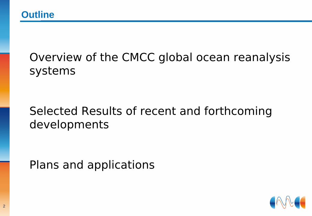
The CMCC Global Ocean (re-)analysis system
Forcing: ERA40 daily fluxes
BG Covariances: Vertical EOFs from Model
In Situ Data: WOD05, WOCE, ARGO, etc.
(Temperature and Salinity)
Ocean Model: OPA8.2/ORCA2
Masina et al. (2011)
Assimilation:Reduced Order OI
(Bellucci et al. 2007)
YEAR 2008
4
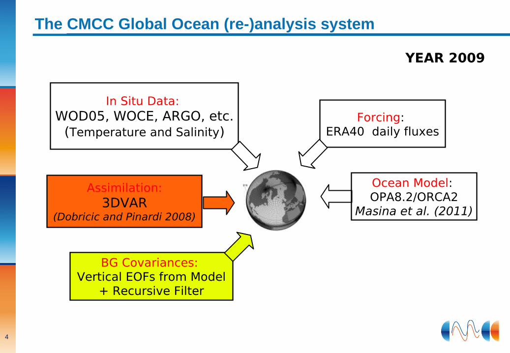
The CMCC Global Ocean (re-)analysis system
Forcing: ERA40 daily fluxes
BG Covariances: Vertical EOFs from Model
+ Recursive Filter
In Situ Data: WOD05, WOCE, ARGO, etc.
(Temperature and Salinity)
Ocean Model: OPA8.2/ORCA2
Masina et al. (2011)
Assimilation:3DVAR
(Dobricic and Pinardi 2008)
YEAR 2009
5
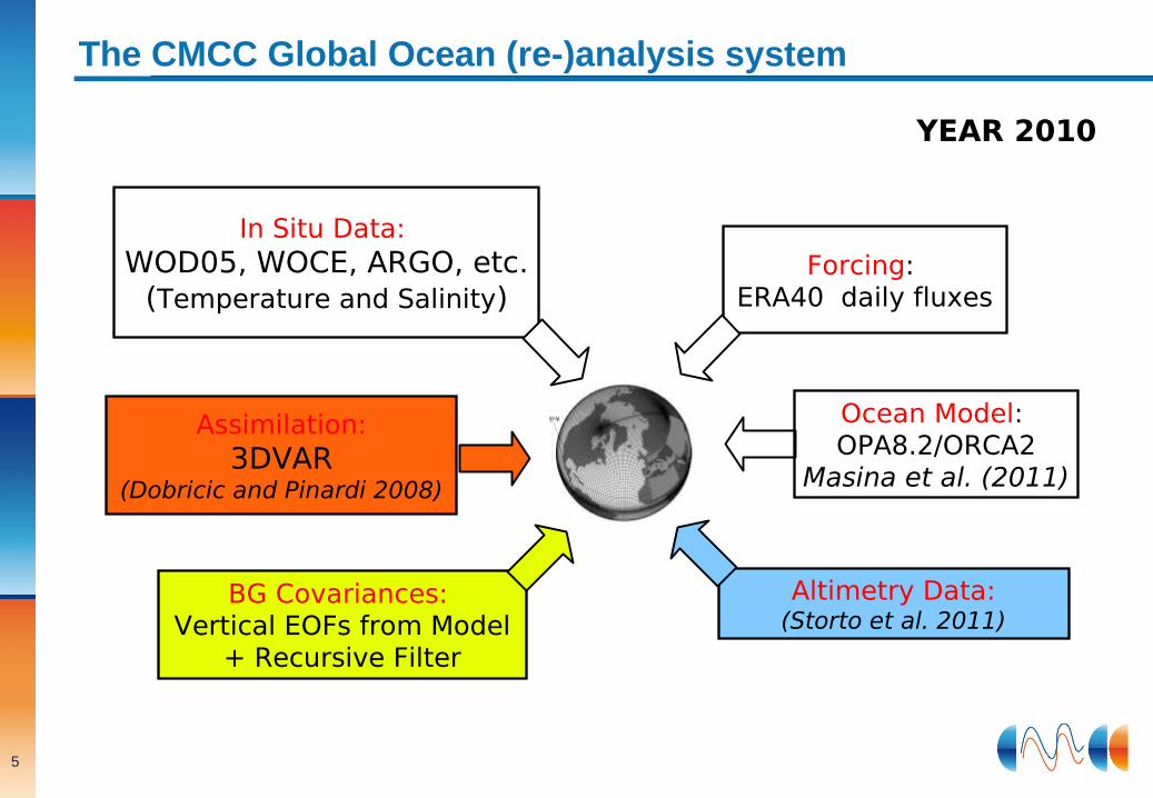
The CMCC Global Ocean (re-)analysis system
Forcing: ERA40 daily fluxes
BG Covariances: Vertical EOFs from Model
+ Recursive Filter
In Situ Data: WOD05, WOCE, ARGO, etc.
(Temperature and Salinity)
Ocean Model: OPA8.2/ORCA2
Masina et al. (2011)
Assimilation:3DVAR
(Dobricic and Pinardi 2008)
Altimetry Data:(Storto et al. 2011)
YEAR 2010
6
The CMCC Global Ocean (re-)analysis system
Forcing: ERA-Interim
CORE bulk formulas
BG Covariances: Vertical EOFs from Model
+ Recursive Filter
In Situ Data: WOD05, WOCE, ARGO, etc.
(Temperature and Salinity)
Ocean Model: NEMO3.2/ORCA025(Storto et al. 2012)
Assimilation:3DVAR
(Dobricic and Pinardi 2008)
Altimetry Data:(Storto et al. 2011)
YEAR 2011
7
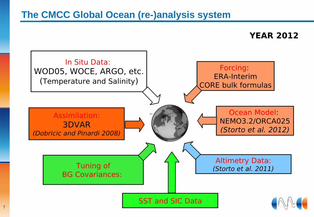
The CMCC Global Ocean (re-)analysis system
Forcing: ERA-Interim
CORE bulk formulas
Tuning ofBG Covariances:
In Situ Data: WOD05, WOCE, ARGO, etc.
(Temperature and Salinity)
Ocean Model: NEMO3.2/ORCA025(Storto et al. 2012)
Assimilation:3DVAR
(Dobricic and Pinardi 2008)
Altimetry Data:(Storto et al. 2011)
YEAR 2012
SST and SIC Data
8
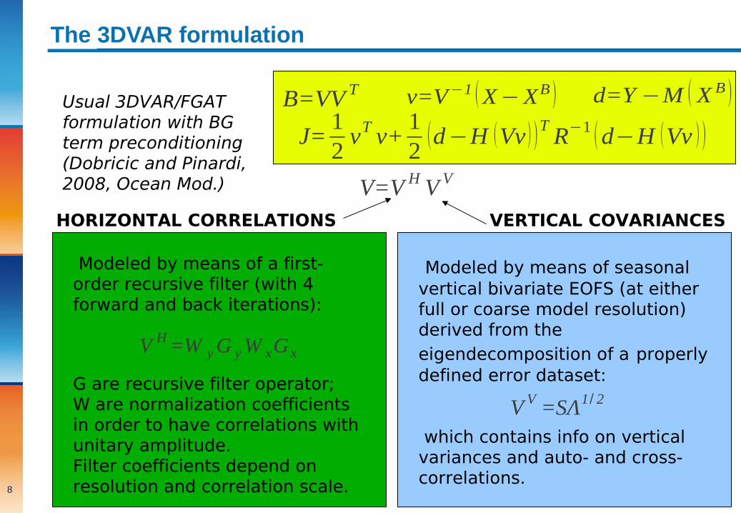
The 3DVAR formulation
V=V H V V
Modeled by means of a first-order recursive filter (with 4 forward and back iterations):
Modeled by means of seasonal vertical bivariate EOFS (at either full or coarse model resolution) derived from the eigendecomposition of a properly defined error dataset:
V H=W yG yW xG x
V V =SΛ1/ 2G are recursive filter operator;W are normalization coefficients in order to have correlations with unitary amplitude.Filter coefficients depend on resolution and correlation scale.
HORIZONTAL CORRELATIONS VERTICAL COVARIANCES
which contains info on vertical variances and auto- and cross- correlations.
B=VV T v=V−1 (X−XB )
J=12
vT v+12
(d−H (Vv ) )T R−1 (d−H (Vv ) )
Usual 3DVAR/FGATformulation with BG term preconditioning(Dobricic and Pinardi,2008, Ocean Mod.)
d=Y −M ( X B )
9
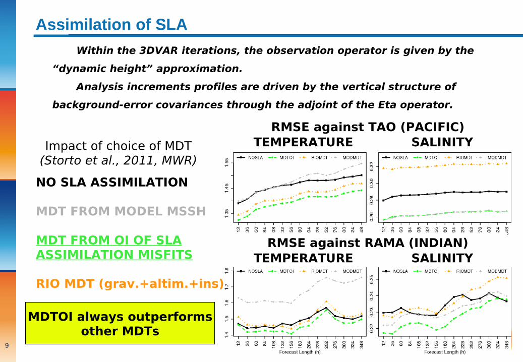
Assimilation of SLA
Within the 3DVAR iterations, the observation operator is given by the
“dynamic height” approximation.
Analysis increments profiles are driven by the vertical structure of
background-error covariances through the adjoint of the Eta operator.
Impact of choice of MDT(Storto et al., 2011, MWR)
TEMPERATURE SALINITYRMSE against TAO (PACIFIC)
TEMPERATURE SALINITYRMSE against RAMA (INDIAN)
NO SLA ASSIMILATION
MDT FROM MODEL MSSH
MDT FROM OI OF SLA ASSIMILATION MISFITS
RIO MDT (grav.+altim.+ins)
MDTOI always outperformsother MDTs
10
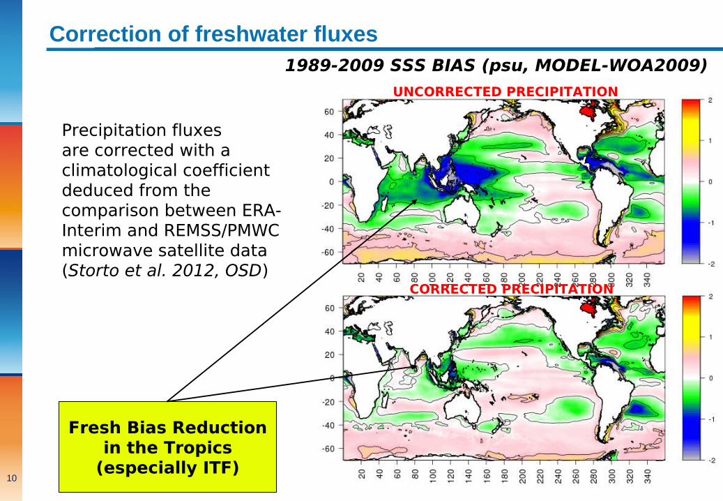
Correction of freshwater fluxes1989-2009 SSS BIAS (psu, MODEL-WOA2009)
Precipitation fluxesare corrected with a climatological coefficient deduced from the comparison between ERA-Interim and REMSS/PMWC microwave satellite data(Storto et al. 2012, OSD)
UNCORRECTED PRECIPITATION
CORRECTED PRECIPITATION
Fresh Bias Reductionin the Tropics
(especially ITF)
11
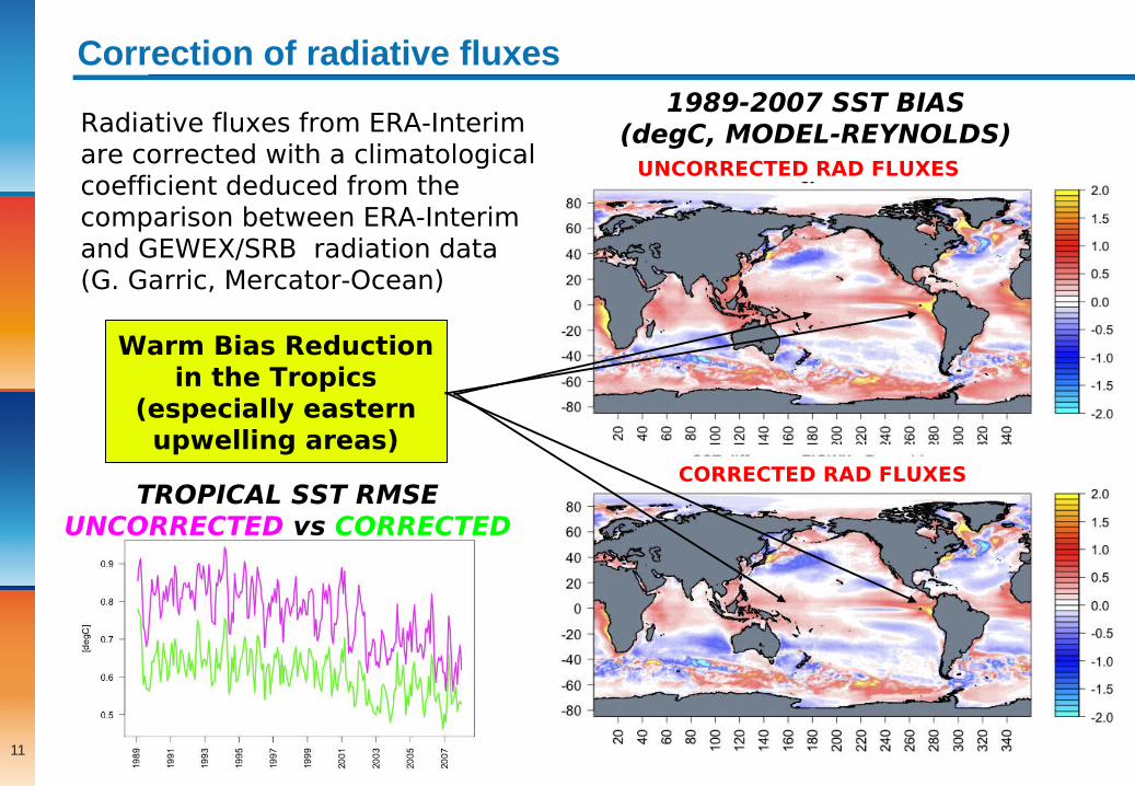
Correction of radiative fluxes
Radiative fluxes from ERA-Interim are corrected with a climatological coefficient deduced from the comparison between ERA-Interim and GEWEX/SRB radiation data (G. Garric, Mercator-Ocean)
1989-2007 SST BIAS(degC, MODEL-REYNOLDS)
UNCORRECTED RAD FLUXES
CORRECTED RAD FLUXES
Warm Bias Reductionin the Tropics
(especially easternupwelling areas)
TROPICAL SST RMSEUNCORRECTED vs CORRECTED
12
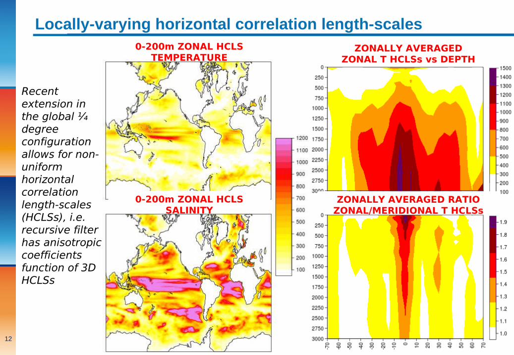
Locally-varying horizontal correlation length-scales
Recent extension in the global ¼ degree configuration allows for non-uniform horizontal correlation length-scales (HCLSs), i.e. recursive filter has anisotropic coefficients function of 3D HCLSs
ZONALLY AVERAGEDZONAL T HCLSs vs DEPTH
ZONALLY AVERAGED RATIO ZONAL/MERIDIONAL T HCLSs
0-200m ZONAL HCLSTEMPERATURE
0-200m ZONAL HCLSSALINITY
13
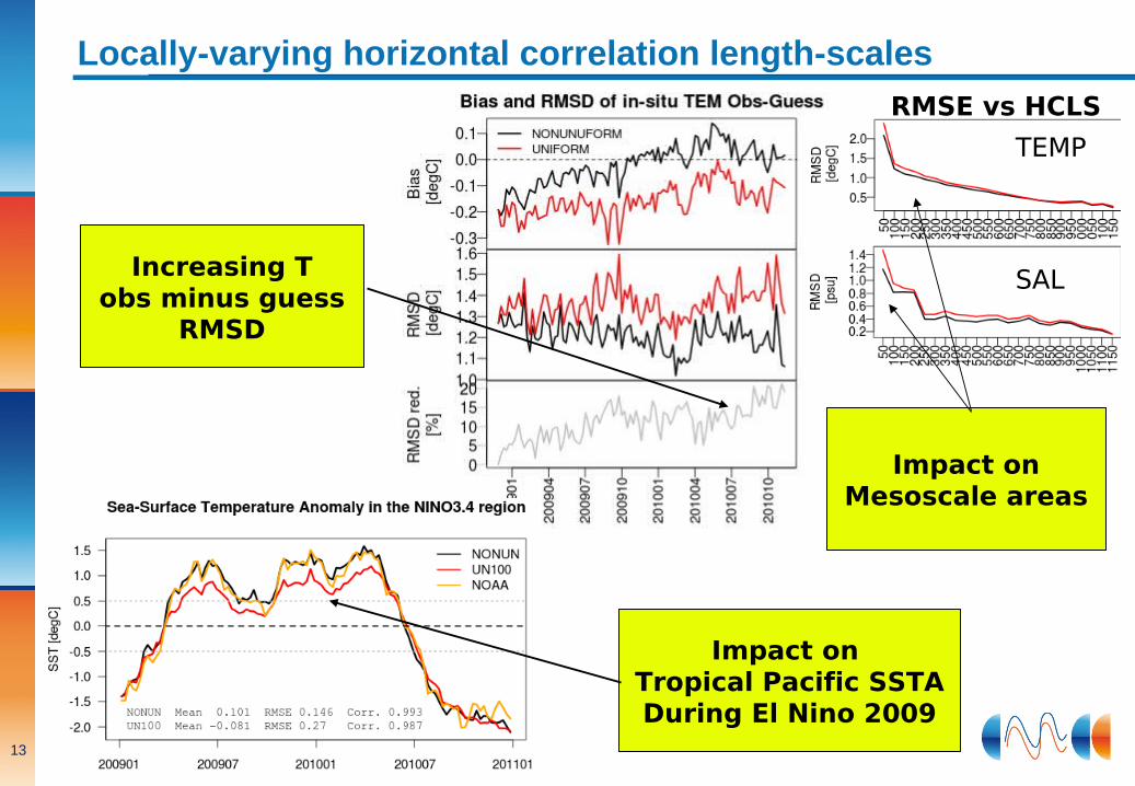
Locally-varying horizontal correlation length-scales
Impact on Tropical Pacific SSTADuring El Nino 2009
Increasing Tobs minus guess
RMSD
Impact onMesoscale areas
TEMP
SAL
RMSE vs HCLS
14
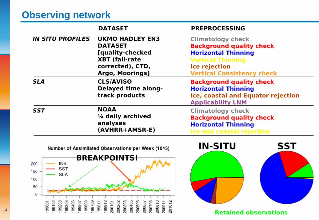
Observing networkDATASET
IN SITU PROFILES UKMO HADLEY EN3 DATASET[quality-checked XBT (fall-rate corrected), CTD, Argo, Moorings]
SLA CLS/AVISODelayed time along-track products
SST NOAA¼ daily archived analyses(AVHRR+AMSR-E)
PREPROCESSING
Climatology checkBackground quality checkHorizontal ThinningVertical ThinningIce rejectionVertical Consistency check
Background quality checkHorizontal ThinningIce, coastal and Equator rejectionApplicability LNM
Climatology checkBackground quality checkHorizontal ThinningIce and coastal rejection
IN-SITU SST
Retained observations
BREAKPOINTS!
15
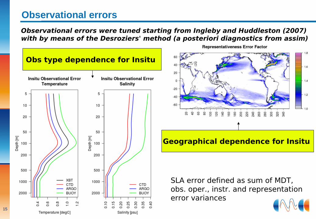
Observational errors
SLA error defined as sum of MDT, obs. oper., instr. and representation error variances
Obs type dependence for Insitu
Geographical dependence for Insitu
Observational errors were tuned starting from Ingleby and Huddleston (2007) with by means of the Desroziers' method (a posteriori diagnostics from assim)
16
Status and plans
PRODUCTION (¼ degree resolution)
2 Releases have been produced for MyOcean (CGLORSV1 and CGLORSV2) for the period 1991-2010 (1993-2009 officially released)> Bernard Barnier's presentation tomorrow 1 Release that fixes some problems in CGLORSV2 (sea-ice and SLA assimilation) is under production
MAIN CONCERNS
T/S Vertical covariances may produce significant model drifts Optimal Initialization/Spinup for the reanalysis still needs to be addressed
PLANS
Use of ensemble-derived sets of vertical covariances; Vertical localization operator to avoid spurious vertical correlations;
17
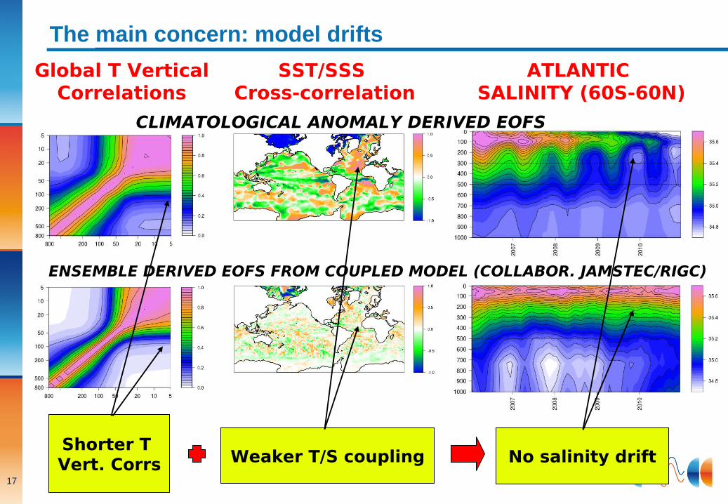
The main concern: model drifts
ATLANTIC SALINITY (60S-60N)
SST/SSS Cross-correlation
Global T VerticalCorrelations
CLIMATOLOGICAL ANOMALY DERIVED EOFS
ENSEMBLE DERIVED EOFS FROM COUPLED MODEL (COLLABOR. JAMSTEC/RIGC)
Shorter T Vert. Corrs Weaker T/S coupling No salinity drift
18
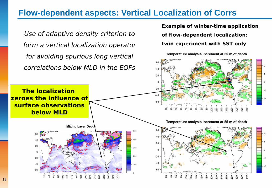
Flow-dependent aspects: Vertical Localization of Corrs
Use of adaptive density criterion to
form a vertical localization operator
for avoiding spurious long vertical
correlations below MLD in the EOFs
Example of winter-time application
of flow-dependent localization:
twin experiment with SST only
The localization zeroes the influence ofsurface observations
below MLD
19
Further developments we're working on
- Detailed EOFS comparison and implement simple large-scale bias-correction schemes for model drift mitigations;
- A balance operator (“barotropic operator”) that will allow to correct u,v further to T,S. It will be possible to test the assimilation of drifter trajectories;
- Variational correction of the Mean Dynamic Topography to improve SLA assimilation;
- Multilinear bias correction of space-borne observations and reformulation of background quality check to account for actual observation misfit distributions;
- Sea-ice assimilation brought into 3DVAR (now nudging);
20
Main Usage of CMCC ocean reanalyses
Estimate the interannual-to-decadal upper ocean variability (Masina el al. 2011); Provide ocean initial condition for seasonal (Alessandri et al, 2010) and decadal forecating activities (Bellucci et al, under review); Give a contribution to the GSOP/GODAE Ocean View initiative on global ocean analyses intercomparison; Provide a set of oceanic variables for the validation and comparison with the CMCC Earth System Model (Vichi et al, 2011)
21
Main Usage of CMCC ocean reanalyses
Estimate the interannual-to-decadal upper ocean variability (Masina el al. 2011); Provide ocean initial condition for seasonal (Alessandri et al, 2010) and decadal forecating activities (Bellucci et al, under review); Give a contribution to the GSOP/GODAE Ocean View initiative on global ocean analyses intercomparison; Provide a set of oceanic variables for the validation and comparison with the CMCC Earth System Model (Vichi et al, 2011)
Thank you!
22
General configuration of C-GLORS
DATA ASSIMILATION
3DVAR/FGAT formulation with weekly correction of (T,S) “Direct initialization” Horizontal correlations via first-order recursive filter Vertical covariances via seasonal bivariate EOFs of T, S Assimilation of SLA through the adjoint of the “dynamic height” formula
OCEAN GENERAL CIRCULATION MODEL
NEMO (3.2.1) 0.25 L50 + LIM2 Sea-Ice Model CORE bulk formulas with 3-hourly ERA-Interim turbulent fluxes and daily freshwater and radiative fluxes (solar diurnal cycle analytically imposed) Correction of radiative fluxes with GEWEX/SRB Correction of precipitation fluxes with REMSS/PMWC Nudging to NOAA sea-ice concentration data (15-day relaxation scale)
INITIALIZATION
Free run initialized from 1979 (ERA-Interim) from ocean at rest and WOA climatology Assimilation switched on in 1989
23
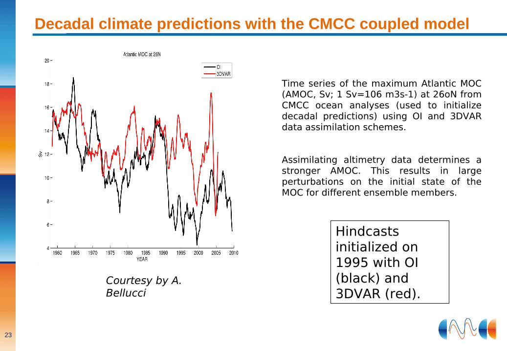
Decadal climate predictions with the CMCC coupled model
Time series of the maximum Atlantic MOC (AMOC, Sv; 1 Sv=106 m3s-1) at 26oN from CMCC ocean analyses (used to initialize decadal predictions) using OI and 3DVAR data assimilation schemes.
Assimilating altimetry data determines a stronger AMOC. This results in large perturbations on the initial state of the MOC for different ensemble members.
Hindcasts initialized on 1995 with OI (black) and 3DVAR (red).
Courtesy by A. Bellucci