The CLUE model

Hands-on exercises

Course material Peter Verburg

January 2010

2

CLUE model - background Introduction The Conversion of Land Use and its Effects modelling framework (CLUE) was developed to simulate land use change using empirically quantified relations between land use and its driving factors in combination with dynamic modelling of competition between land use types. The model was developed for the national and continental level and applications for Central America, Ecuador, China and Java, Indonesia are available. For study areas with such a large extent the spatial resolution for analysis was coarse and, as a result, each land use is represented by assigning the relative cover of each land use type to the pixels. Land use data for study areas with a relatively small spatial extent is often based on land use maps or remote sensing images that denote land use types respectively by homogeneous polygons or classified pixels. This results in only one dominant land use type occupying one unit of analysis. Because of the differences in data representation and other features that are typical for regional applications, the CLUE model cannot directly be applied at the regional scale. Therefore the modelling approach has been modified and is now called CLUE-S (the Conversion of Land Use and its Effects at Small regional extent). CLUE-S is specifically developed for the spatially explicit simulation of land use change based on an empirical analysis of location suitability combined with the dynamic simulation of competition and interactions between the spatial and temporal dynamics of land use systems. More information on the development of the CLUE-S model can be found in Verburg et al. (2002) and Verburg and Veldkamp (2003). The more recent versions of the CLUE model: Dyna-CLUE (Verburg and Overmars, 2009) and CLUE-Scanner include new methodological advances. Model structure The model is sub-divided into two distinct modules, namely a non-spatial demand module and a spatially explicit allocation procedure (Figure 1). The non-spatial module calculates the area change for all land use types at the aggregate level. Within the second part of the model these demands are translated into land use changes at different locations within the study region using a raster-based system. The user-interface of the CLUE-S model only supports the spatial allocation of land use change. For the land use demand module different model specifications are possible ranging from simple trend extrapolations to complex economic models. The choice for a specific model is very much dependent on the nature of the most important land use conversions taking place within the study area and the scenarios that need to be considered. The results from the demand module need to specify, on a yearly basis, the area covered by the different land use types, which is a direct input for the allocation module.

3

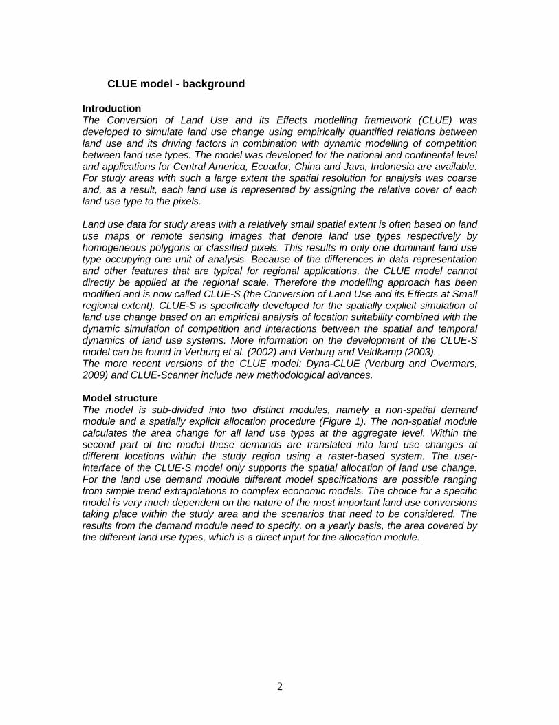
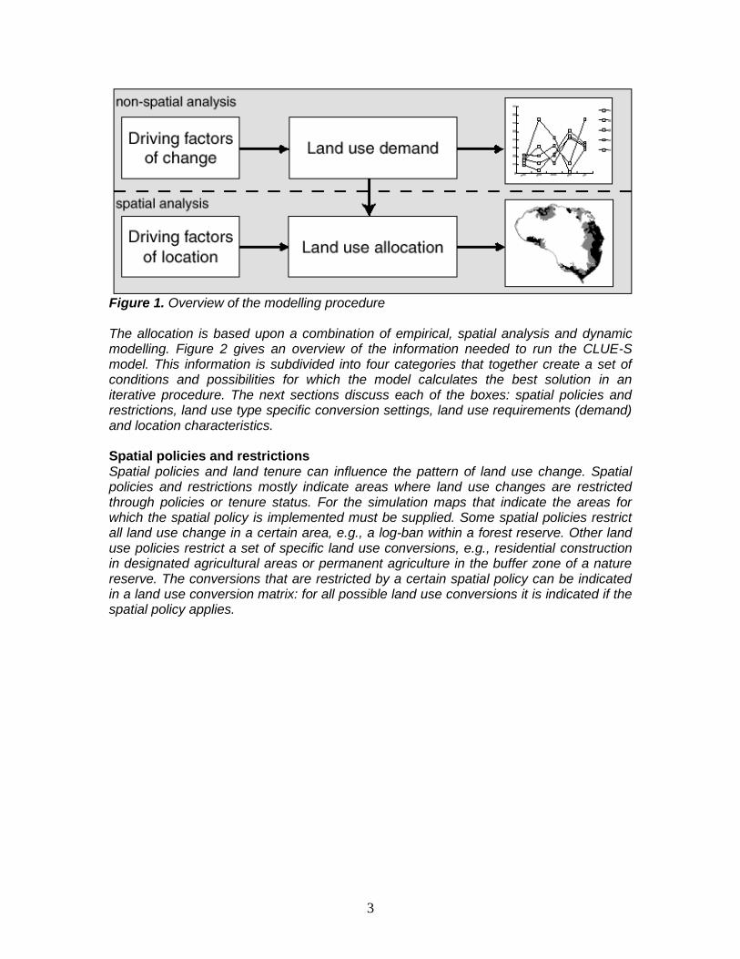
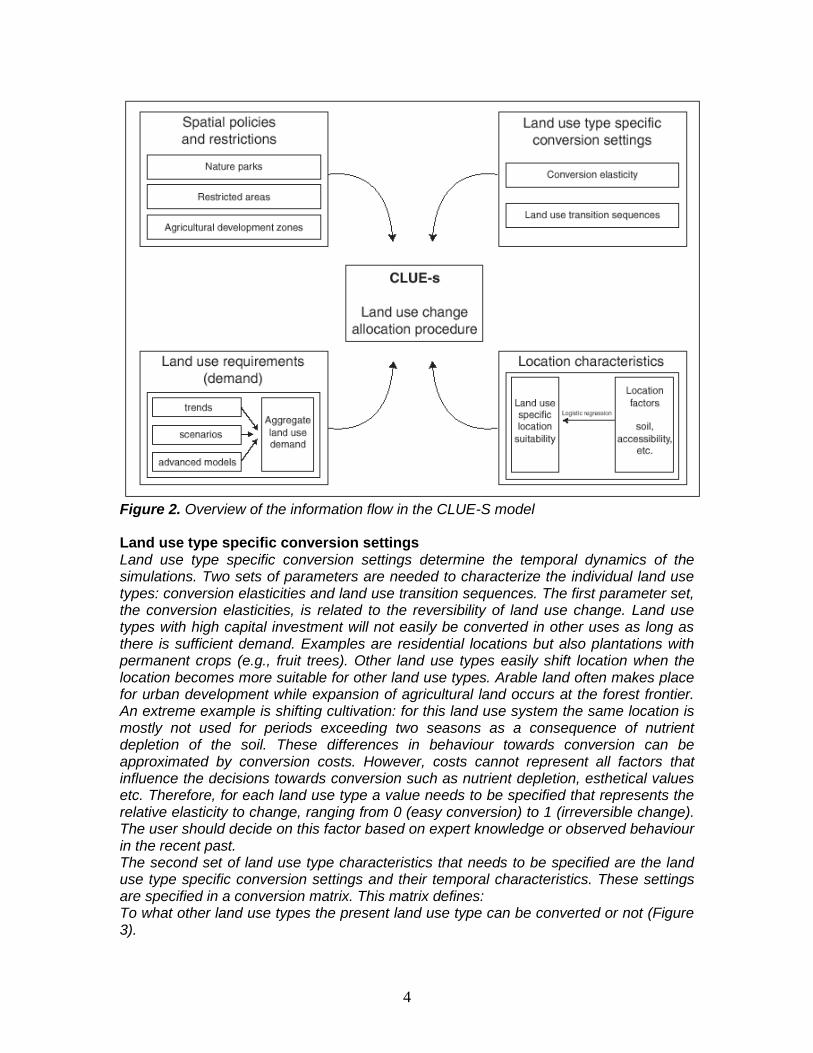
Figure 1. Overview of the modelling procedure The allocation is based upon a combination of empirical, spatial analysis and dynamic modelling. Figure 2 gives an overview of the information needed to run the CLUE-S model. This information is subdivided into four categories that together create a set of conditions and possibilities for which the model calculates the best solution in an iterative procedure. The next sections discuss each of the boxes: spatial policies and restrictions, land use type specific conversion settings, land use requirements (demand) and location characteristics. Spatial policies and restrictions Spatial policies and land tenure can influence the pattern of land use change. Spatial policies and restrictions mostly indicate areas where land use changes are restricted through policies or tenure status. For the simulation maps that indicate the areas for which the spatial policy is implemented must be supplied. Some spatial policies restrict all land use change in a certain area, e.g., a log-ban within a forest reserve. Other land use policies restrict a set of specific land use conversions, e.g., residential construction in designated agricultural areas or permanent agriculture in the buffer zone of a nature reserve. The conversions that are restricted by a certain spatial policy can be indicated in a land use conversion matrix: for all possible land use conversions it is indicated if the spatial policy applies.

4

Figure 2. Overview of the information flow in the CLUE-S model Land use type specific conversion settings Land use type specific conversion settings determine the temporal dynamics of the simulations. Two sets of parameters are needed to characterize the individual land use types: conversion elasticities and land use transition sequences. The first parameter set, the conversion elasticities, is related to the reversibility of land use change. Land use types with high capital investment will not easily be converted in other uses as long as there is sufficient demand. Examples are residential locations but also plantations with permanent crops (e.g., fruit trees). Other land use types easily shift location when the location becomes more suitable for other land use types. Arable land often makes place for urban development while expansion of agricultural land occurs at the forest frontier. An extreme example is shifting cultivation: for this land use system the same location is mostly not used for periods exceeding two seasons as a consequence of nutrient depletion of the soil. These differences in behaviour towards conversion can be approximated by conversion costs. However, costs cannot represent all factors that influence the decisions towards conversion such as nutrient depletion, esthetical values etc. Therefore, for each land use type a value needs to be specified that represents the relative elasticity to change, ranging from 0 (easy conversion) to 1 (irreversible change). The user should decide on this factor based on expert knowledge or observed behaviour in the recent past. The second set of land use type characteristics that needs to be specified are the land use type specific conversion settings and their temporal characteristics. These settings are specified in a conversion matrix. This matrix defines: To what other land use types the present land use type can be converted or not (Figure 3).

5

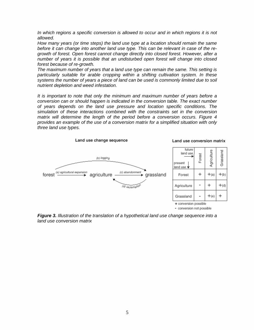
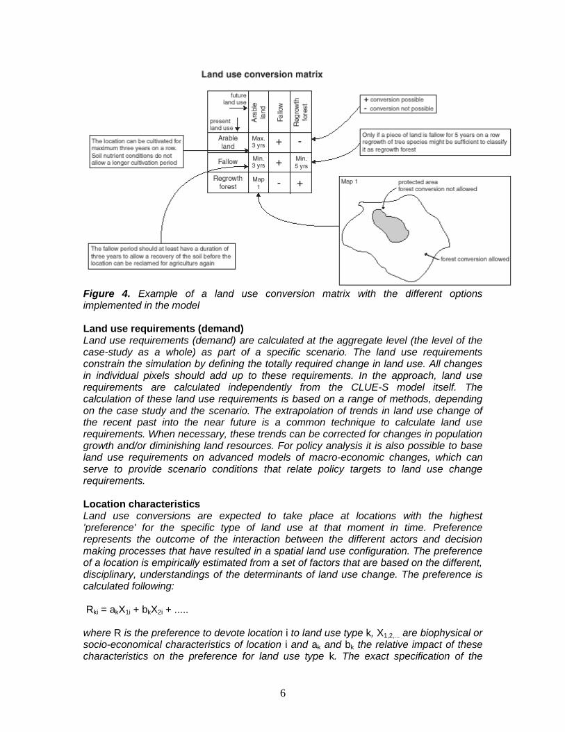
In which regions a specific conversion is allowed to occur and in which regions it is not allowed. How many years (or time steps) the land use type at a location should remain the same before it can change into another land use type. This can be relevant in case of the re-growth of forest. Open forest cannot change directly into closed forest. However, after a number of years it is possible that an undisturbed open forest will change into closed forest because of re-growth. The maximum number of years that a land use type can remain the same. This setting is particularly suitable for arable cropping within a shifting cultivation system. In these systems the number of years a piece of land can be used is commonly limited due to soil nutrient depletion and weed infestation. It is important to note that only the minimum and maximum number of years before a conversion can or should happen is indicated in the conversion table. The exact number of years depends on the land use pressure and location specific conditions. The simulation of these interactions combined with the constraints set in the conversion matrix will determine the length of the period before a conversion occurs. Figure 4 provides an example of the use of a conversion matrix for a simplified situation with only three land use types.

Figure 3. Illustration of the translation of a hypothetical land use change sequence into a land use conversion matrix

6

Figure 4. Example of a land use conversion matrix with the different options implemented in the model Land use requirements (demand) Land use requirements (demand) are calculated at the aggregate level (the level of the case-study as a whole) as part of a specific scenario. The land use requirements constrain the simulation by defining the totally required change in land use. All changes in individual pixels should add up to these requirements. In the approach, land use requirements are calculated independently from the CLUE-S model itself. The calculation of these land use requirements is based on a range of methods, depending on the case study and the scenario. The extrapolation of trends in land use change of the recent past into the near future is a common technique to calculate land use requirements. When necessary, these trends can be corrected for changes in population growth and/or diminishing land resources. For policy analysis it is also possible to base land use requirements on advanced models of macro-economic changes, which can serve to provide scenario conditions that relate policy targets to land use change requirements. Location characteristics Land use conversions are expected to take place at locations with the highest 'preference' for the specific type of land use at that moment in time. Preference represents the outcome of the interaction between the different actors and decision making processes that have resulted in a spatial land use configuration. The preference of a location is empirically estimated from a set of factors that are based on the different, disciplinary, understandings of the determinants of land use change. The preference is calculated following: Rki = akX1i + bkX2i + ..... where R is the preference to devote location i to land use type k, X1,2,... are biophysical or socio-economical characteristics of location i and ak and bk the relative impact of these characteristics on the preference for land use type k. The exact specification of the

7

model should be based on a thorough review of the processes important to the spatial allocation of land use in the studied region. A statistical model can be developed as a binomial logit model of two choices: convert location i into land use type k or not. The preference Rki is assumed to be the underlying response of this choice. However, the preference Rki cannot be observed or measured directly and has therefore to be calculated has a probability. The function that relates these probabilities with the biophysical and socio-economic location characteristics is defined in a logit model following:

where Pi is the probability of a grid cell for the occurrence of the considered land use type on location i and the X's are the location factors. The coefficients (β) are estimated through logistic regression using the actual land use pattern as dependent variable. This method is similar to econometric analysis of land use change, which is very common in deforestation studies. In econometric studies the assumed behaviour is profit maximization, which limits the location characteristics to (agricultural) economic factors. In the study areas is assumed that locations are devoted to the land use type with the highest 'suitability'. 'Suitability' includes the monetary profit, but can also include cultural and other factors that lead to deviations from (economic) rational behaviour in land allocation. This assumption makes it possible to include a wide variety of location characteristics or their proxies to estimate the logit function that defines the relative probabilities for the different land use types. Most of these location characteristics relate to the location directly, such as soil characteristics and altitude. However, land management decisions for a certain location are not always based on location specific characteristics alone. Conditions at other levels, e.g., the household, community or administrative level can influence the decisions as well. These factors are represented by accessibility measures, indicating the position of the location relative to important regional facilities, such as the market and by the use of spatially lagged variables. A spatially lagged measure of the population density approximates the regionally population pressure for the location instead of only representing the population living at the location itself. Allocation procedure When all input is provided the CLUE-S model calculates, with discrete time steps, the most likely changes in land use given the before described restrictions and suitabilities. The allocation procedure is summarized in Figure 5. The following steps are taken to allocate the changes in land use: The first step includes the determination of all grid cells that are allowed to change. Grid cells that are either part of a protected area or presently under a land use type that is not allowed to change are excluded from further calculation. Also the locations where certain conversions are not allowed due to the specification of the conversion matrix are identified. For each grid cell i the total probability (TPROPi,u) is calculated for each of the land use types u according to:

innii

i

i XXXP

PLog ,,22,110 ......

1

8

where Pi,u is the suitability of location i for land use type u (based on the logit model), ELASu is the conversion elasticity for land use u and ITERu is an iteration variable that is specific to the land use type and indicative for the relative competitive strength of the land use type. ELASu, the land use type specific elasticity to change value, is only added if grid-cell i is already under land use type u in the year considered. A preliminary allocation is made with an equal value of the iteration variable (ITERu) for all land use types by allocating the land use type with the highest total probability for the considered grid cell. Conversions that are not allowed according to the conversion matrix are not allocated. This allocation process will cause a certain number of grid cells to change land use. The total allocated area of each land use is now compared to the land use requirements (demand). For land use types where the allocated area is smaller than the demanded area the value of the iteration variable is increased. For land use types for which too much is allocated the value is decreased. Through this procedure it is possible that the local suitability based on the location factors is overruled by the iteration variable due to the differences in regional demand. The procedure followed balances the bottom-up allocation based on location suitability and the top-down allocation based on regional demand. Steps 2 to 4 are repeated as long as the demands are not correctly allocated. When allocation equals demand the final map is saved and the calculations can continue for the next time step. Some of the allocated changes are irreversible while others are dependent on the changes in earlier time steps. Therefore, the simulations tend to result in complex, non-linear changes in land use pattern, characteristic for complex systems.

Figure 5. Flow chart of the allocation module of the CLUE-S model

uuuiui ITERELASPTPROP ,,

9

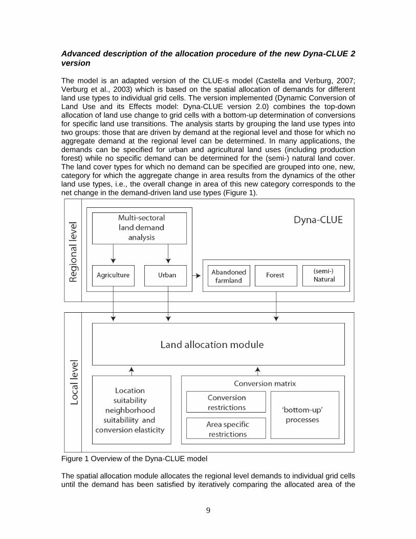
Advanced description of the allocation procedure of the new Dyna-CLUE 2 version The model is an adapted version of the CLUE-s model (Castella and Verburg, 2007; Verburg et al., 2003) which is based on the spatial allocation of demands for different land use types to individual grid cells. The version implemented (Dynamic Conversion of Land Use and its Effects model: Dyna-CLUE version 2.0) combines the top-down allocation of land use change to grid cells with a bottom-up determination of conversions for specific land use transitions. The analysis starts by grouping the land use types into two groups: those that are driven by demand at the regional level and those for which no aggregate demand at the regional level can be determined. In many applications, the demands can be specified for urban and agricultural land uses (including production forest) while no specific demand can be determined for the (semi-) natural land cover. The land cover types for which no demand can be specified are grouped into one, new, category for which the aggregate change in area results from the dynamics of the other land use types, i.e., the overall change in area of this new category corresponds to the net change in the demand-driven land use types (Figure 1).

Figure 1 Overview of the Dyna-CLUE model The spatial allocation module allocates the regional level demands to individual grid cells until the demand has been satisfied by iteratively comparing the allocated area of the

10

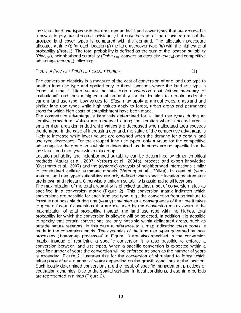
individual land use types with the area demanded. Land cover types that are grouped in a new category are allocated individually but only the sum of the allocated area of the grouped land cover types is compared with the demand. The allocation procedure allocates at time (t) for each location (i) the land use/cover type (lu) with the highest total probability (Ptoti,t,lu). The total probability is defined as the sum of the location suitability (Ploci,t,lu), neighborhood suitability (Pnbhi,t,lu), conversion elasticity (elaslu) and competitive advantage (compt,lu) following: Ptoti,t,lu = Ploci,t,lu + Pnbhi,t,lu + elaslu + compt,lu (1) The conversion elasticity is a measure of the cost of conversion of one land use type to another land use type and applied only to those locations where the land use type is found at time t. High values indicate high conversion cost (either monetary or institutional) and thus a higher total probability for the location to remain under the current land use type. Low values for Elaslu may apply to annual crops, grassland and similar land use types while high values apply to forest, urban areas and permanent crops for which high costs of establishment have been made. The competitive advantage is iteratively determined for all land use types during an iterative procedure. Values are increased during the iteration when allocated area is smaller than area demanded while values are decreased when allocated area exceeds the demand. In the case of increasing demand, the value of the competitive advantage is likely to increase while lower values are obtained when the demand for a certain land use type decreases. For the grouped land use types, only a value for the competitive advantage for the group as a whole is determined, as demands are not specified for the individual land use types within this group. Location suitability and neighborhood suitability can be determined by either empirical methods (Aguiar et al., 2007; Verburg et al., 2004b), process and expert knowledge (Overmars et al., 2007) and the (dynamic) analysis of neighborhood interactions similar to constrained cellular automata models (Verburg et al., 2004a). In case of (semi-)natural land use types suitabilities are only defined when specific location requirements are known and relevant. Otherwise a uniform suitability is assigned to all locations. The maximization of the total probability is checked against a set of conversion rules as specified in a conversion matrix (Figure 2). This conversion matrix indicates which conversions are possible for each land use type, e.g., the conversion from agriculture to forest is not possible during one (yearly) time step as a consequence of the time it takes to grow a forest. Conversions that are excluded by the conversion matrix overrule the maximization of total probability. Instead, the land use type with the highest total probability for which the conversion is allowed will be selected. In addition it is possible to specify that certain conversions are only possible within delineated areas, such as outside nature reserves. In this case a reference to a map indicating these zones is made in the conversion matrix. The dynamics of the land use types governed by local processes (‘bottom-up processes’ in Figure 1) are also specified in the conversion matrix. Instead of restricting a specific conversion it is also possible to enforce a conversion between land use types. When a specific conversion is expected within a specific number of years the conversion will be enforced as soon as the number of years is exceeded. Figure 2 illustrates this for the conversion of shrubland to forest which takes place after a number of years depending on the growth conditions at the location. Such locally determined conversions are the result of specific management practices or vegetation dynamics. Due to the spatial variation in local conditions, these time periods are represented in a map (Figure 2).

11

Figure 2. Simplified land cover conversion matrix indicating the possible conversions during one time step of the simulation Locally determined conversions will, to some extent, interfere with the allocation of the other land use types that are driven by the regional demands due to changes in conversion elasticity upon locally determined conversions, i.e., the conversion to agriculture is less difficult for recently abandoned agricultural land than for shrubland. The resulting conversion trajectories will cause intricate interactions between the spatial and temporal dynamics of the simulation.

The specification of the model for different land use types, location suitability, conversion elasticity and conversion matrix is dependent on the specific case study area, spatial and temporal scale and the purpose of the model. The following section illustrates the functioning of the model by a specification of the model for the simulation of land use for the 27 countries of the European Union at a spatial resolution of 1 km2 for the time period 2000-2030. Implementation of the Dyna-CLUE model for Europe The application of the model for Europe includes 16 different land use types (Annex 3). Although the land use types area derived from a land cover map (CLC/CORINE, (EEA, 2005)), they also represent, to some extent, the use of the land cover. Therefore, we

12

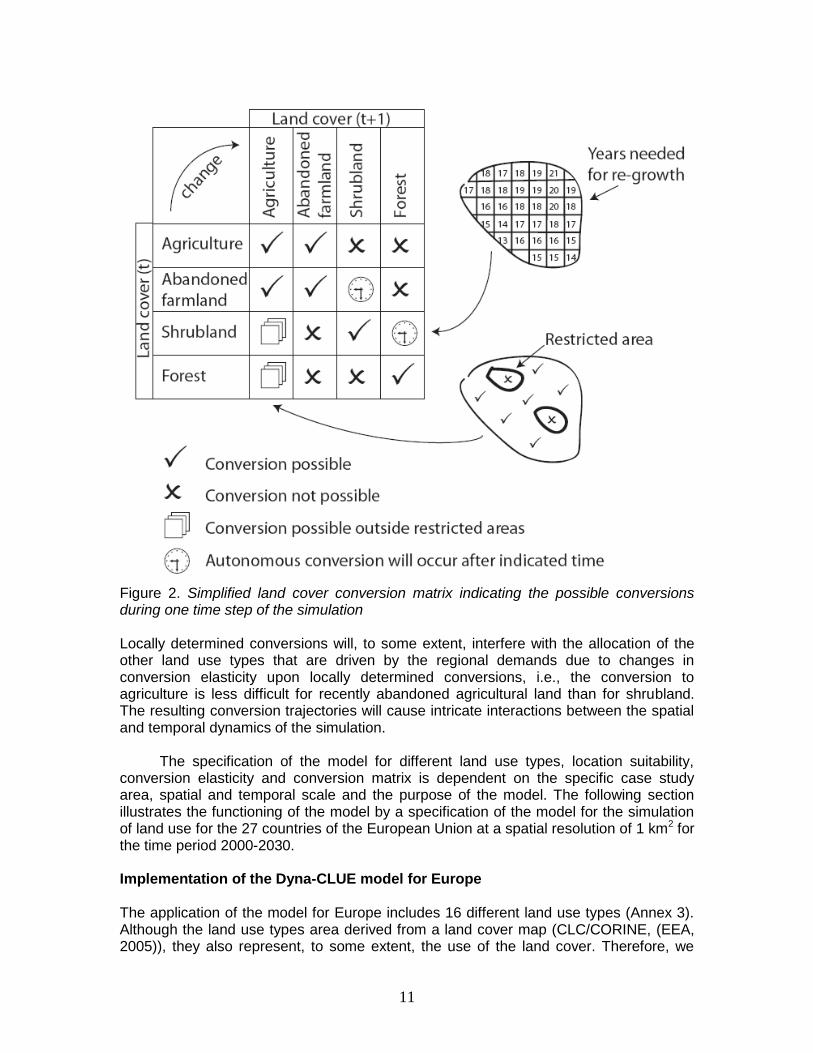
refer to ‘land use types’ in the following. The land use types are subdivided into 3 categories. The first category includes land use types for which a demand is calculated at the level of individual member states by a macro-economic, multi-sector model accounting for global trade and agricultural policy (Meijl et al., 2006; Verburg et al., 2008a) in combination with a simple projection model for urbanization. The second category contains land use types for which the area is expected to be more or less constant in time due to the inability to use these lands for agricultural or urban purposes, or strict protection to avoid conversion. The third category contains land use types the conversions of which are determined by local conditions, especially the regeneration of natural vegetation. Land use types in this group are recently abandoned arable land, recently abandoned grassland, (semi-)natural vegetation and forest. The land use types in this category are grouped into one single group the area of which is a result of the dynamics of the agricultural and urban land use types. Agricultural decline will increase the area of this group while agricultural expansion and urbanization will occur at the cost of this group. The protected areas for nature conservation determine the minimum area allocated to these (semi-) natural land uses. The conceptual transitions between the land use types in this group are shown in Figure 3. Upon abandonment of agricultural land regeneration/succession of (semi-)natural vegetation takes place depending on the local conditions that favor or retard the establishment and growth of natural vegetation.

Figure 3 Schematization of the land use/cover transitions upon abandonment of agricultural land The subdivision of the regrowth of natural vegetation into three stages of succession is arbitrary since succession is a continuous process. However, the three stages were chosen because of their clear morphological and functional differences and frequent use in studies of succession on abandoned farmland (Pueyo and Beguería, 2007). Occasional grazing on abandoned farmlands, which is common practice in many parts of Europe, may retard the transition to shrubs and trees (González-Martínez and Bravo, 2001; Tasser et al., 2007; Tzanopoulos et al., 2007). Also, in densely populated areas alternative uses may occupy former farmland areas, e.g., hobby farming and horse-

13

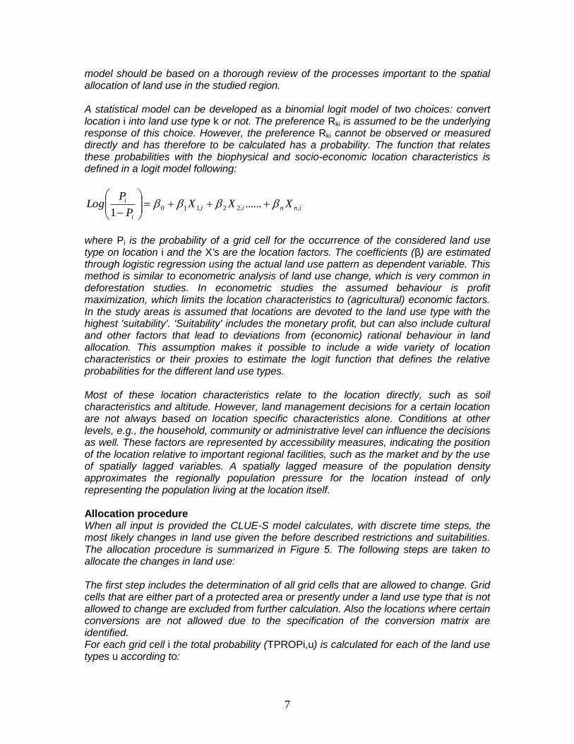
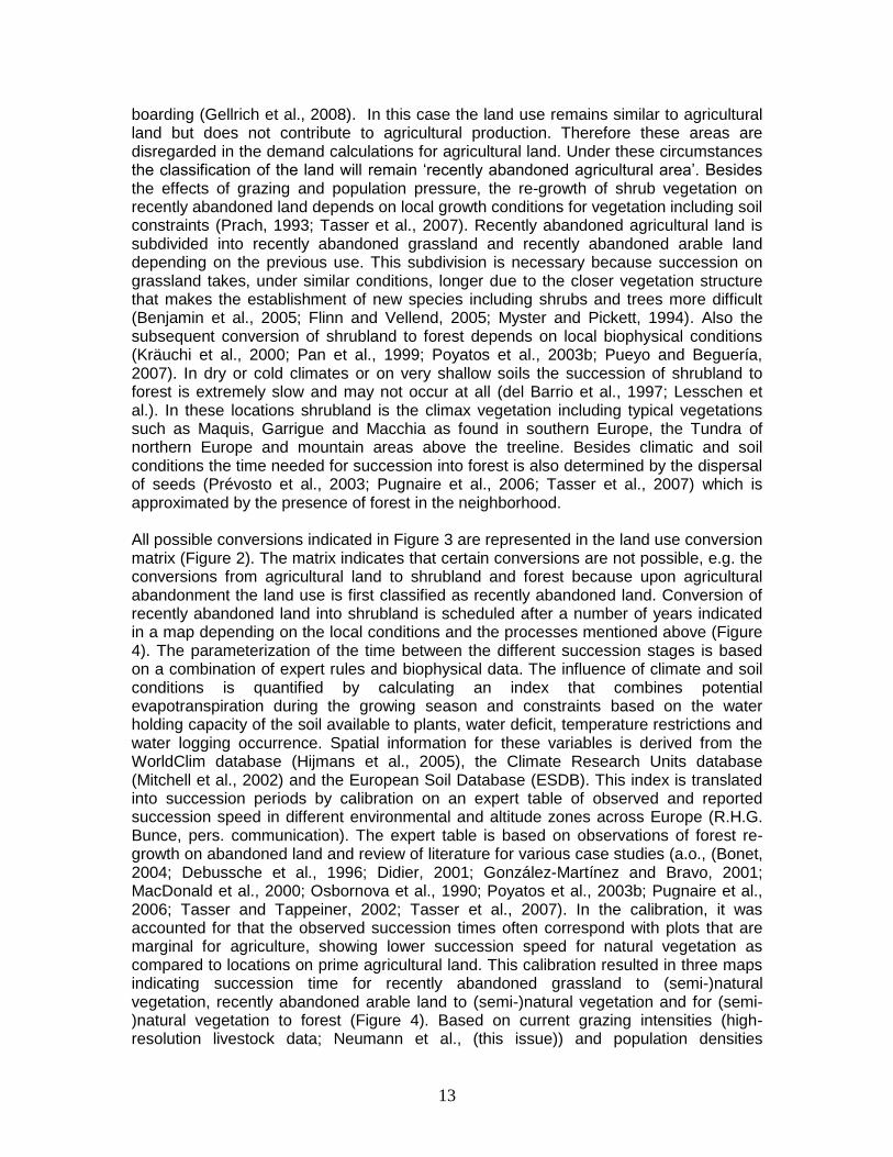
boarding (Gellrich et al., 2008). In this case the land use remains similar to agricultural land but does not contribute to agricultural production. Therefore these areas are disregarded in the demand calculations for agricultural land. Under these circumstances the classification of the land will remain ‘recently abandoned agricultural area’. Besides the effects of grazing and population pressure, the re-growth of shrub vegetation on recently abandoned land depends on local growth conditions for vegetation including soil constraints (Prach, 1993; Tasser et al., 2007). Recently abandoned agricultural land is subdivided into recently abandoned grassland and recently abandoned arable land depending on the previous use. This subdivision is necessary because succession on grassland takes, under similar conditions, longer due to the closer vegetation structure that makes the establishment of new species including shrubs and trees more difficult (Benjamin et al., 2005; Flinn and Vellend, 2005; Myster and Pickett, 1994). Also the subsequent conversion of shrubland to forest depends on local biophysical conditions (Kräuchi et al., 2000; Pan et al., 1999; Poyatos et al., 2003b; Pueyo and Beguería, 2007). In dry or cold climates or on very shallow soils the succession of shrubland to forest is extremely slow and may not occur at all (del Barrio et al., 1997; Lesschen et al.). In these locations shrubland is the climax vegetation including typical vegetations such as Maquis, Garrigue and Macchia as found in southern Europe, the Tundra of northern Europe and mountain areas above the treeline. Besides climatic and soil conditions the time needed for succession into forest is also determined by the dispersal of seeds (Prévosto et al., 2003; Pugnaire et al., 2006; Tasser et al., 2007) which is approximated by the presence of forest in the neighborhood. All possible conversions indicated in Figure 3 are represented in the land use conversion matrix (Figure 2). The matrix indicates that certain conversions are not possible, e.g. the conversions from agricultural land to shrubland and forest because upon agricultural abandonment the land use is first classified as recently abandoned land. Conversion of recently abandoned land into shrubland is scheduled after a number of years indicated in a map depending on the local conditions and the processes mentioned above (Figure 4). The parameterization of the time between the different succession stages is based on a combination of expert rules and biophysical data. The influence of climate and soil conditions is quantified by calculating an index that combines potential evapotranspiration during the growing season and constraints based on the water holding capacity of the soil available to plants, water deficit, temperature restrictions and water logging occurrence. Spatial information for these variables is derived from the WorldClim database (Hijmans et al., 2005), the Climate Research Units database (Mitchell et al., 2002) and the European Soil Database (ESDB). This index is translated into succession periods by calibration on an expert table of observed and reported succession speed in different environmental and altitude zones across Europe (R.H.G. Bunce, pers. communication). The expert table is based on observations of forest re-growth on abandoned land and review of literature for various case studies (a.o., (Bonet, 2004; Debussche et al., 1996; Didier, 2001; González-Martínez and Bravo, 2001; MacDonald et al., 2000; Osbornova et al., 1990; Poyatos et al., 2003b; Pugnaire et al., 2006; Tasser and Tappeiner, 2002; Tasser et al., 2007). In the calibration, it was accounted for that the observed succession times often correspond with plots that are marginal for agriculture, showing lower succession speed for natural vegetation as compared to locations on prime agricultural land. This calibration resulted in three maps indicating succession time for recently abandoned grassland to (semi-)natural vegetation, recently abandoned arable land to (semi-)natural vegetation and for (semi-)natural vegetation to forest (Figure 4). Based on current grazing intensities (high-resolution livestock data; Neumann et al., (this issue)) and population densities

14

(LandScanTM Global Population Database; Oak Ridge National Laboratory) the transition of recently abandoned agricultural land to shrubland was retarded to represent the effects of grazing and alternative uses under conditions of high population pressure. Grazing in areas with more than 30 livestock units/km2 was assumed to retard succession by 5 years while in zones with more than 75 livestock units/km2 succession was retarded by 10 years. In areas with high population pressure (identified by calculating a population potential map) the succession was assumed to be retarded by between 5 and 100 years dependent on the population pressure. Retarding the succession by a long period indicates that succession is unlikely to happen, at least not during the simulation period (2000-2030). In scenarios where active management of natural areas designated under the NATURA2000 scheme was envisioned, the succession time was expected to be two years shorter than elsewhere under similar conditions due to favorable management conditions that enhance the establishment of natural vegetation. Other model settings include the definition of the suitability of locations for agricultural and urban land use types, conversion elasticities and region-specific constraints representing spatial policies and planning. Suitabilities where estimated by logit models using the spatial association of current land use with a wide range of biophysical and socio-economic variables to represent location factors (Verburg et al., 2004b; Verburg et al., 2006b). Conversion elasticities were estimated based on expert knowledge of the conversion costs for different land uses and spatial restrictions included NATURA2000 nature reserves, erosion sensitive locations and ‘less favoured areas’ following the spatial policies included in the scenario description (Westhoek et al., 2006). More specific details on the configuration of the model are provided in Verburg et al. (2008a) and (WUR/MNP, 2008). The application of the model to Europe has illustrated the application of the model in the context of declining agricultural area and regeneration of natural vegetation. The combination of top-down and bottom-up processes in a consistent modeling framework may also be relevant in other areas and for other processes. Examples of possible applications include the dynamics of tropical forest landscapes, where large scale logging as result of global demand for timber and agricultural commodities, interacts with local processes of soil degradation and regeneration of secondary vegetation. Local processes causing soil degradation may prevent future use of these soils and therefore need to be taken into account. In addition, the simulation of low-input agricultural systems with fallow periods as part of the crop rotation may be captured by combining an assessment of the overall demand for agricultural production with local processes of soil fertility dynamics.

15

Figure 4 Number of years needed for the transition of recently abandoned arable land into (semi-) natural vegetation (A) and for the transition of (semi-) natural vegetation into forest (B)

16

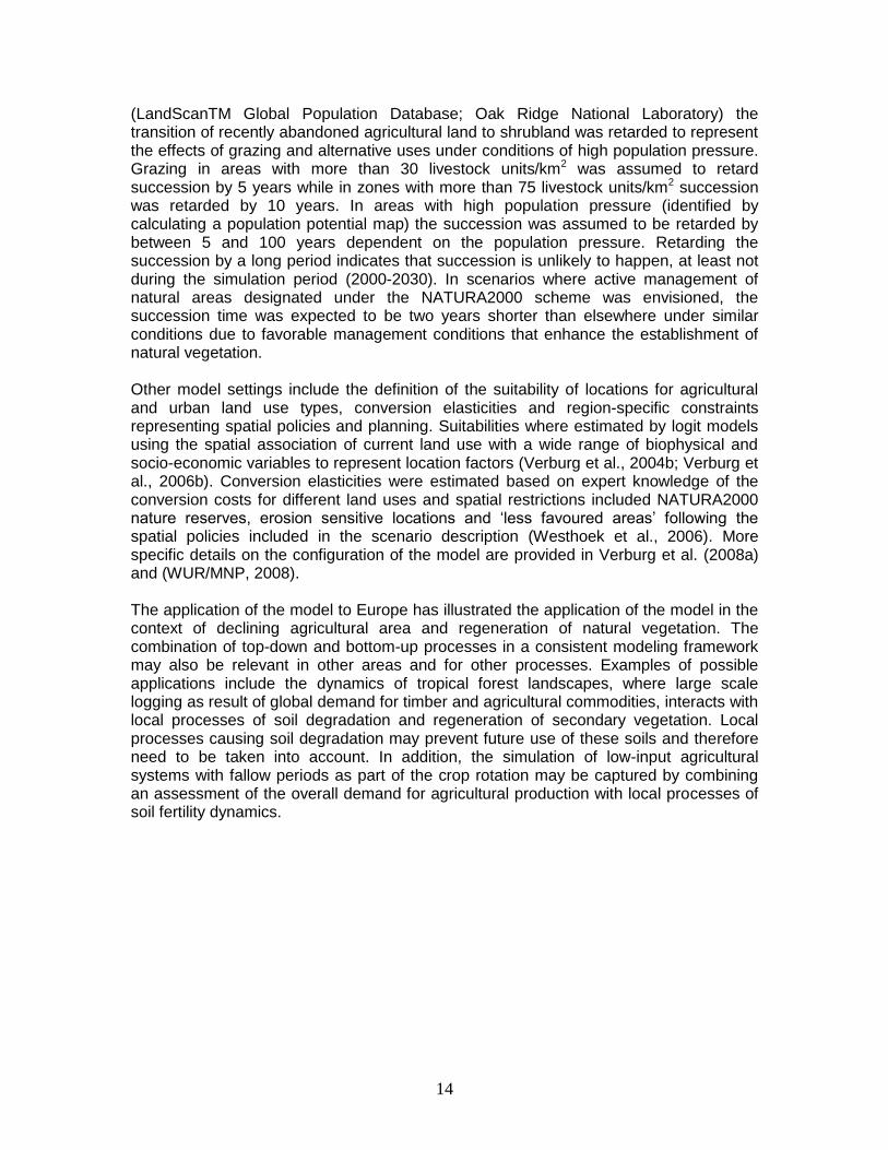
Background of the case study used in the exercises Sibuyan Island For these exercises the case study of Sibuyan Island is used. Sibuyan Island is located in the Romblon Province in the Philippines (Figure 6). The island measures 28 km east to west at its widest point and 24 km north to south, with a land area of approximately 456 km2 surrounded by deep water. Steep mountain slopes covered with forest canopy characterize the island. The land surrounding the high mountains slopes gently to the sea and is mainly used for agricultural, mining and residential activities. The island was selected as a case study because of its very rich biodiversity. About 700 vascular plant species live on Sibuyan Island including 54 endemic to the island and 180 endemic to the Philippine archipelago. Fauna diversity is low, but endemism is high. This makes the island a 'hot spot' for nature conservation and relevant for a detailed study of land use change. For this application a spatial resolution of 250 × 250 meter is used. Five different land use types are distinguished for the simulation (Table 1).

Figure 6. Location of Sibuyan Island

17

Table 1. Land use types on Sibuyan Island

Land use code

Land use type

0 1 2 3 4

Forest Coconut plantations Grassland Rice fields Others (mangrove/beach/villages/etc.)

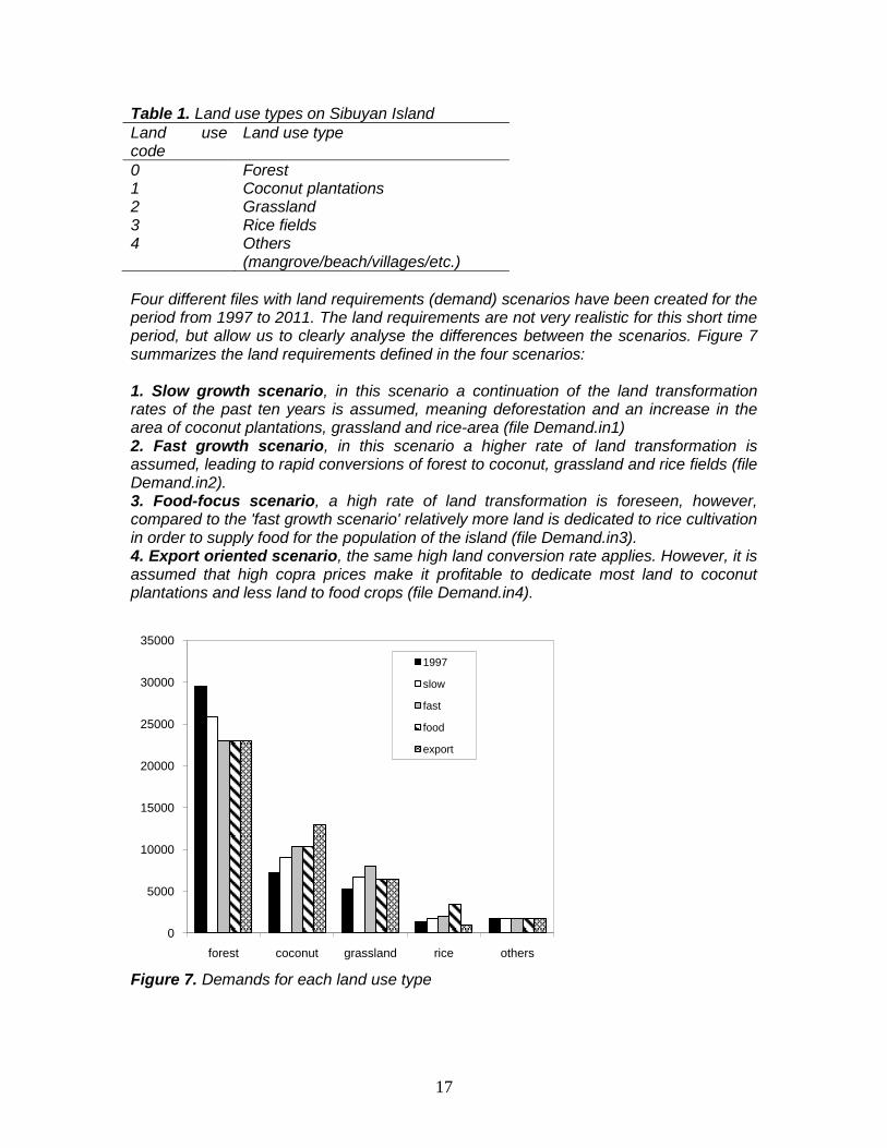
Four different files with land requirements (demand) scenarios have been created for the period from 1997 to 2011. The land requirements are not very realistic for this short time period, but allow us to clearly analyse the differences between the scenarios. Figure 7 summarizes the land requirements defined in the four scenarios: 1. Slow growth scenario, in this scenario a continuation of the land transformation rates of the past ten years is assumed, meaning deforestation and an increase in the area of coconut plantations, grassland and rice-area (file Demand.in1) 2. Fast growth scenario, in this scenario a higher rate of land transformation is assumed, leading to rapid conversions of forest to coconut, grassland and rice fields (file Demand.in2). 3. Food-focus scenario, a high rate of land transformation is foreseen, however, compared to the 'fast growth scenario' relatively more land is dedicated to rice cultivation in order to supply food for the population of the island (file Demand.in3). 4. Export oriented scenario, the same high land conversion rate applies. However, it is assumed that high copra prices make it profitable to dedicate most land to coconut plantations and less land to food crops (file Demand.in4).

Figure 7. Demands for each land use type

0

5000

10000

15000

20000

25000

30000

35000

forest coconut grassland rice others

1997

slow

fast

food

export

18

19

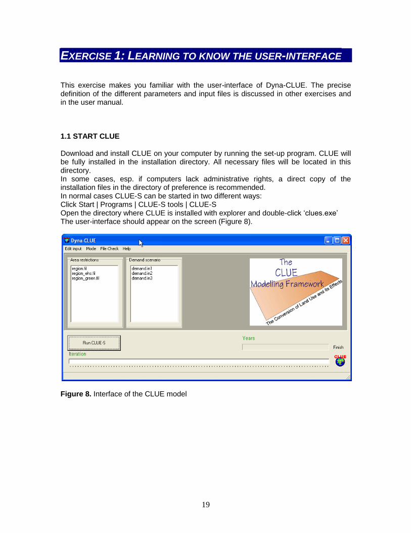
EXERCISE 1: LEARNING TO KNOW THE USER-INTERFACE This exercise makes you familiar with the user-interface of Dyna-CLUE. The precise definition of the different parameters and input files is discussed in other exercises and in the user manual. 1.1 START CLUE Download and install CLUE on your computer by running the set-up program. CLUE will be fully installed in the installation directory. All necessary files will be located in this directory. In some cases, esp. if computers lack administrative rights, a direct copy of the installation files in the directory of preference is recommended. In normal cases CLUE-S can be started in two different ways: Click Start | Programs | CLUE-S tools | CLUE-S Open the directory where CLUE is installed with explorer and double-click ‘clues.exe’ The user-interface should appear on the screen (Figure 8).

Figure 8. Interface of the CLUE model

20

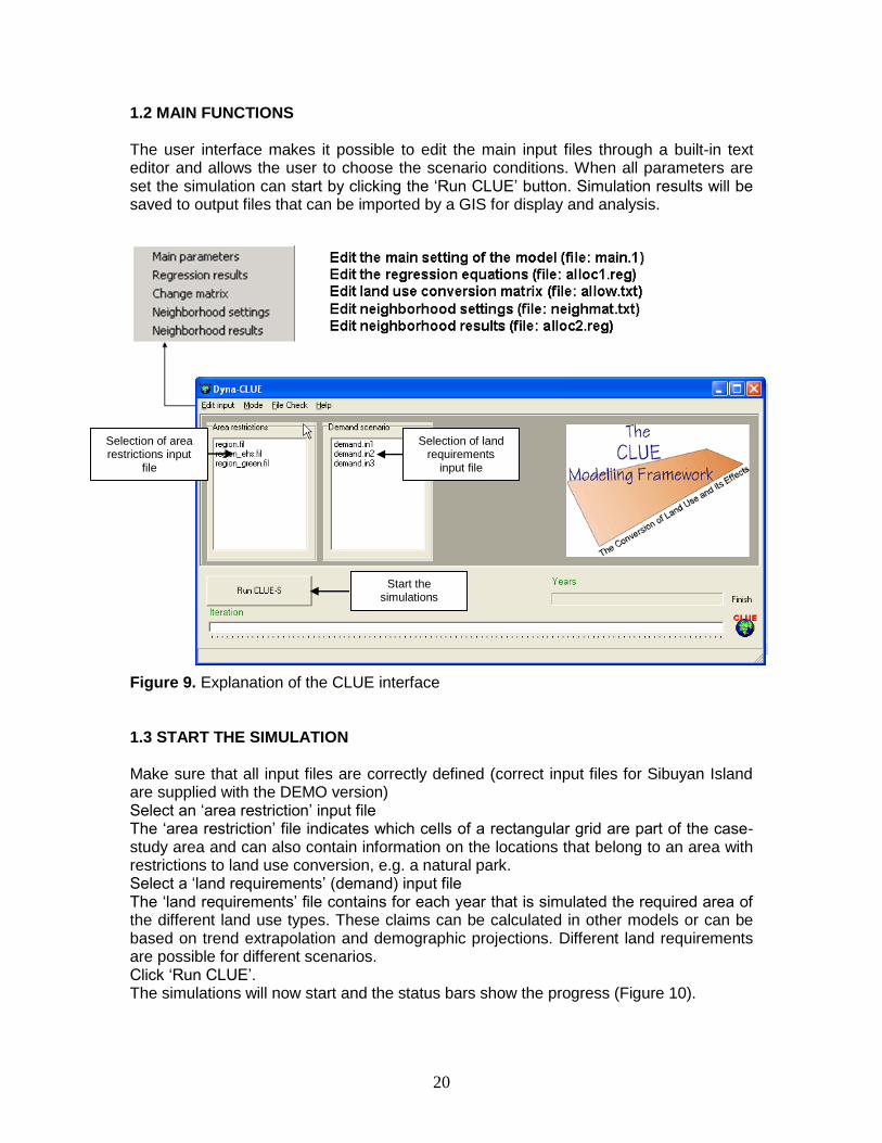
1.2 MAIN FUNCTIONS The user interface makes it possible to edit the main input files through a built-in text editor and allows the user to choose the scenario conditions. When all parameters are set the simulation can start by clicking the ‘Run CLUE’ button. Simulation results will be saved to output files that can be imported by a GIS for display and analysis.

Figure 9. Explanation of the CLUE interface 1.3 START THE SIMULATION Make sure that all input files are correctly defined (correct input files for Sibuyan Island are supplied with the DEMO version) Select an ‘area restriction’ input file The ‘area restriction’ file indicates which cells of a rectangular grid are part of the case-study area and can also contain information on the locations that belong to an area with restrictions to land use conversion, e.g. a natural park. Select a ‘land requirements’ (demand) input file The ‘land requirements’ file contains for each year that is simulated the required area of the different land use types. These claims can be calculated in other models or can be based on trend extrapolation and demographic projections. Different land requirements are possible for different scenarios. Click ‘Run CLUE’. The simulations will now start and the status bars show the progress (Figure 10).

Selection of area restrictions input

file

Selection of land requirements

input file

Start the simulations

21

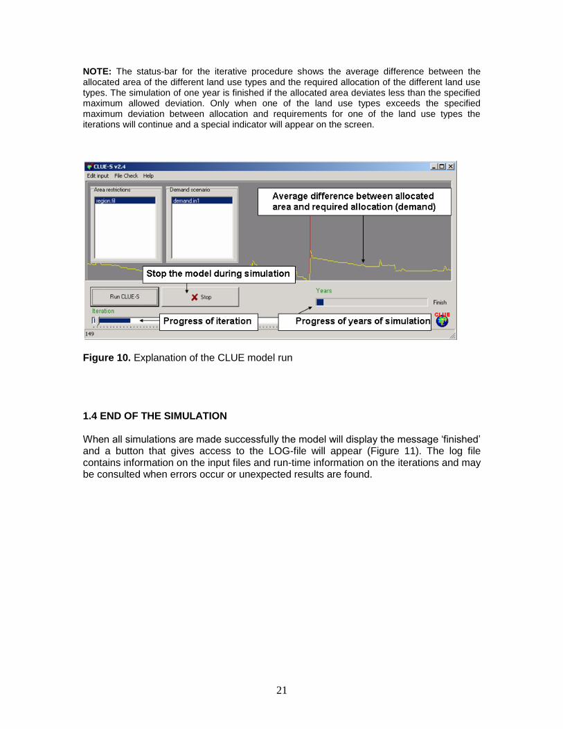
NOTE: The status-bar for the iterative procedure shows the average difference between the allocated area of the different land use types and the required allocation of the different land use types. The simulation of one year is finished if the allocated area deviates less than the specified maximum allowed deviation. Only when one of the land use types exceeds the specified maximum deviation between allocation and requirements for one of the land use types the iterations will continue and a special indicator will appear on the screen.

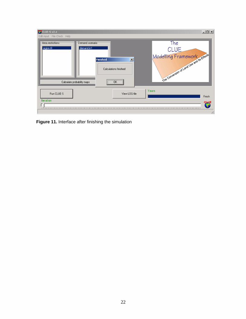
Figure 10. Explanation of the CLUE model run 1.4 END OF THE SIMULATION When all simulations are made successfully the model will display the message ‘finished’ and a button that gives access to the LOG-file will appear (Figure 11). The log file contains information on the input files and run-time information on the iterations and may be consulted when errors occur or unexpected results are found.

22

Figure 11. Interface after finishing the simulation

23

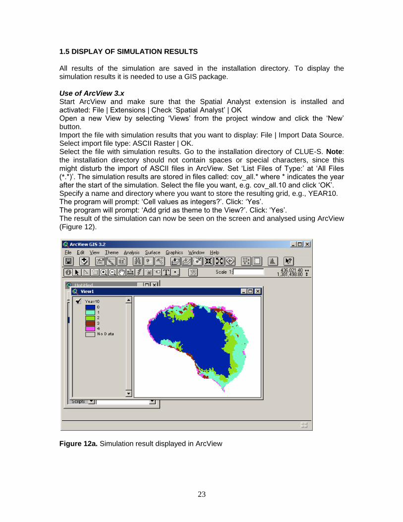
1.5 DISPLAY OF SIMULATION RESULTS All results of the simulation are saved in the installation directory. To display the simulation results it is needed to use a GIS package. Use of ArcView 3.x Start ArcView and make sure that the Spatial Analyst extension is installed and activated: File | Extensions | Check ‘Spatial Analyst’ | OK Open a new View by selecting ‘Views’ from the project window and click the ‘New’ button. Import the file with simulation results that you want to display: File | Import Data Source. Select import file type: ASCII Raster | OK. Select the file with simulation results. Go to the installation directory of CLUE-S. Note: the installation directory should not contain spaces or special characters, since this might disturb the import of ASCII files in ArcView. Set ‘List Files of Type:’ at ‘All Files (*.*)’. The simulation results are stored in files called: cov_all.* where * indicates the year after the start of the simulation. Select the file you want, e.g. cov_all.10 and click ‘OK’. Specify a name and directory where you want to store the resulting grid, e.g., YEAR10. The program will prompt: ‘Cell values as integers?’. Click: ‘Yes’. The program will prompt: ‘Add grid as theme to the View?’. Click: ‘Yes’. The result of the simulation can now be seen on the screen and analysed using ArcView (Figure 12).

Figure 12a. Simulation result displayed in ArcView

24

It is now possible to change the graphical presentation by changing the colors of the map into color that are easily associated with the different land use type. In the demo-version of the model for Sibuyan Island the suggested colours of Table 2 can be used. Use of ArcGIS All results of the simulation are saved in the installation directory. To display the simulation results it is necessary to use a GIS package. For these exercises we will use the ArcMap package with the Spatial Analyst Extension. Follow the steps below to display a land use map generated by the CLUE-S model:

Start ArcMap and make sure that the Spatial Analyst extension is installed and activated: Tools | Extensions | Check ‘Spatial Analyst’ | OK

Import the file with simulation results that you want to display: Conversion Tools | To Raster | ASCII to Raster..

Select the file with simulation results. Go to the installation directory of CLUE-S. Note: the installation directory should not contain spaces or special characters, since this might disturb the import of ASCII files in ArcMap. Set ‘Files of Type:’ to ‘File (*.asc)’. The simulation results are stored in files called: cov_all.*.asc where * indicates the year after the start of the simulation. Select the file you want, e.g. cov_all.10.asc and click ‘OK’.

Specify a name and directory where you want to store the resulting grid, e.g., year10. Cell values are integers.

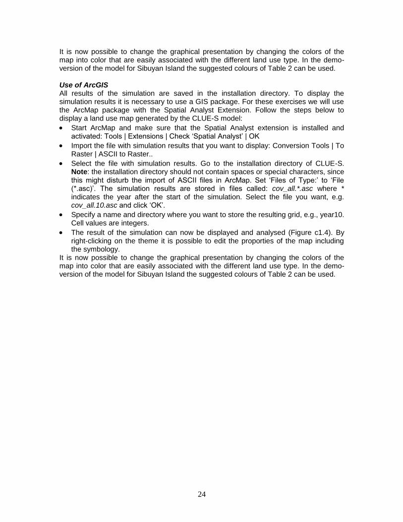
The result of the simulation can now be displayed and analysed (Figure c1.4). By right-clicking on the theme it is possible to edit the proporties of the map including the symbology.

It is now possible to change the graphical presentation by changing the colors of the map into color that are easily associated with the different land use type. In the demo-version of the model for Sibuyan Island the suggested colours of Table 2 can be used.

25

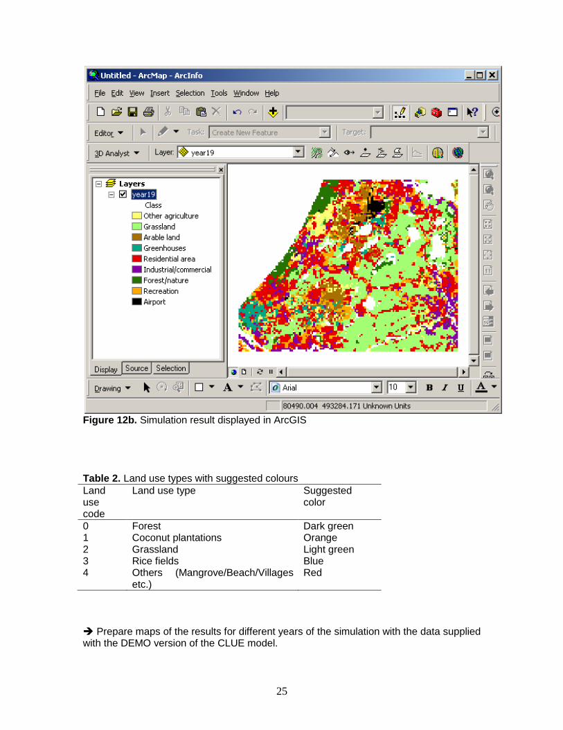
Figure 12b. Simulation result displayed in ArcGIS Table 2. Land use types with suggested colours

Land use code

Land use type Suggested color

0 1 2 3 4

Forest Coconut plantations Grassland Rice fields Others (Mangrove/Beach/Villages etc.)

Dark green Orange Light green Blue Red

Prepare maps of the results for different years of the simulation with the data supplied with the DEMO version of the CLUE model.

26

27

EXERCISE 2: SIMULATING DIFFERENT SCENARIOS OF

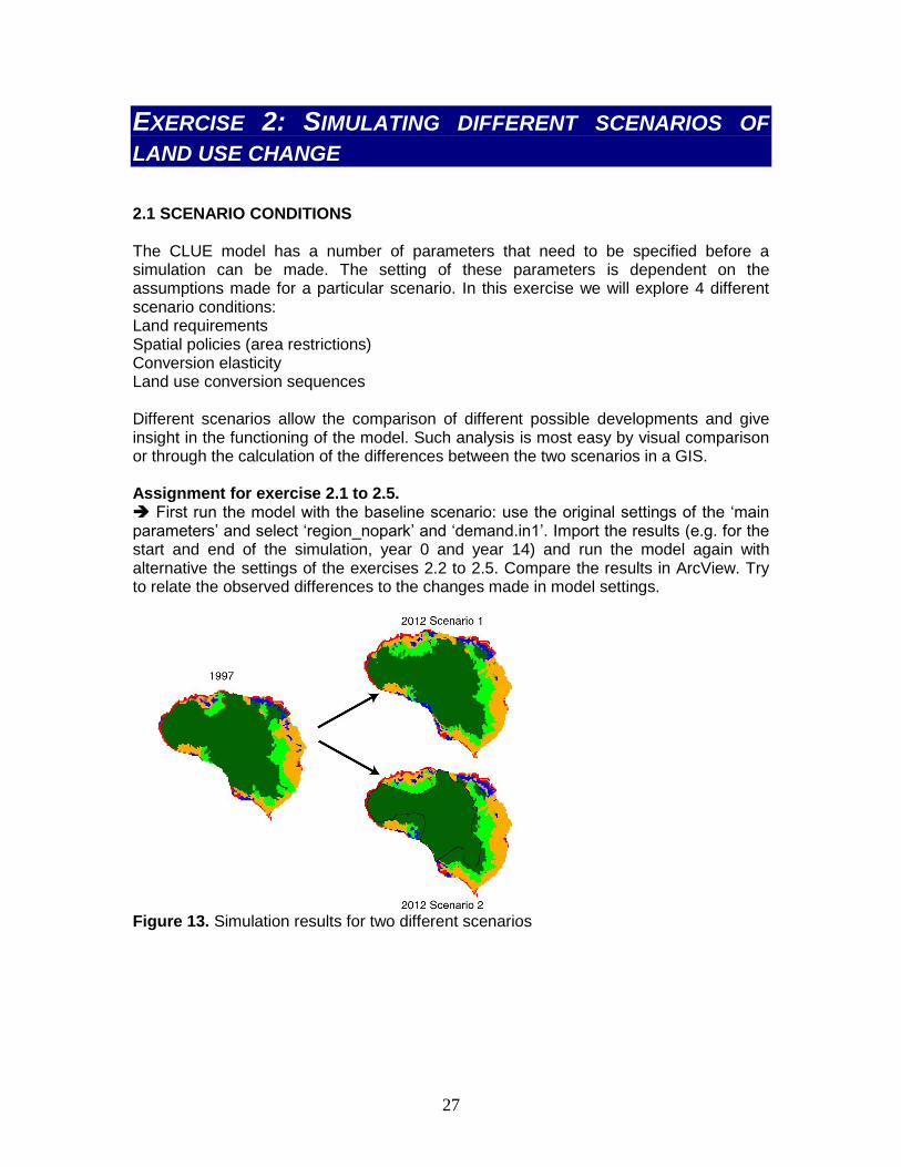
LAND USE CHANGE 2.1 SCENARIO CONDITIONS The CLUE model has a number of parameters that need to be specified before a simulation can be made. The setting of these parameters is dependent on the assumptions made for a particular scenario. In this exercise we will explore 4 different scenario conditions: Land requirements Spatial policies (area restrictions) Conversion elasticity Land use conversion sequences Different scenarios allow the comparison of different possible developments and give insight in the functioning of the model. Such analysis is most easy by visual comparison or through the calculation of the differences between the two scenarios in a GIS. Assignment for exercise 2.1 to 2.5. First run the model with the baseline scenario: use the original settings of the ‘main parameters’ and select ‘region_nopark’ and ‘demand.in1’. Import the results (e.g. for the start and end of the simulation, year 0 and year 14) and run the model again with alternative the settings of the exercises 2.2 to 2.5. Compare the results in ArcView. Try to relate the observed differences to the changes made in model settings.

Figure 13. Simulation results for two different scenarios

28

2.2 LAND REQUIREMENTS The land requirements are input to the model. For each year of the simulation these requirements determine the total area of each land use type that needs to be allocated by the model. The iterative procedure will ensure that the difference between allocated land cover and the land requirements is minimized. Land requirements are calculated independently from the CLUE model itself, which calculates the spatial allocation of land use change only. The calculation of the land use requirements can be based on a range of methods, depending on the case study and the scenario. The extrapolation of trends of land use change of the recent past into the near future is a common technique to calculate the land use requirements. When necessary, these trends can be corrected for changes in population growth and/or diminishing land resources. For policy analysis it is also possible to base the land use requirements on advanced models of macro-economic changes, which can serve to provide scenario conditions that relate policy targets to land use change requirements. Simulating scenarios with different land requirements Four different files with land requirements are provided with the model for the period from 1997 to 2011. The land requirements in these scenarios are not very realistic for this short time period but allow us to clearly analyse the differences between the scenarios. The scenarios are based on the following assumptions: demand.in1: Slow growth scenario, in this scenario a continuation of the land transformation rates of the past ten years is assumed, meaning deforestation and an increase in the area of coconut plantations, grassland and rice fields. demand.in2: Fast growth scenario, in this scenario a higher rate of land transformation is assumed, leading to rapid conversions of forest to coconut, grassland and rice fields. demand.in3: Food-focus scenario, a high rate of land transformation is foreseen, however, compared to the 'fast growth scenario' relatively more land is dedicated to rice cultivation in order to supply food for the population of the island. demand.in4: Export oriented scenario, the same high land conversion rate applies. However, it is assumed that high copra prices make it profitable to dedicate most land to coconut plantations and less land to food crops. Select one of the land requirement scenarios and run the model keeping all other settings equal to the first run of the model. Analyse the results wit ArcView through displaying the land use pattern at the start of the simulation and at the end of the simulation. Repeat this for another scenario of land requirements and compare the results. NOTE: Each simulation, the model will overwrite the results of a previous simulation. If you want to save the results, rename the output files or move the output files to another directory.

Define your own scenario by generating a new land requirements input file for CLUE-S. Follow the steps below: Open Microsoft Excel to facilitate the calculations. Specify for each year (1997-2011) the land requirements of the different land use types in a table following the specifications below:

29

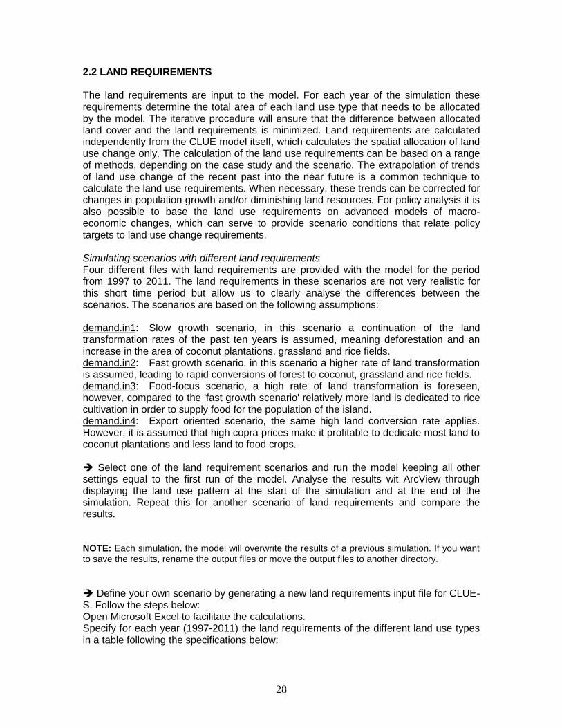
Each row indicates a year; each column a land use type following the order of the land use coding. Make sure to include also the land requirements for 1997 (year 0). These should be similar to the land use map of 1997 (29518.75, 7237.5, 5243.75, 1400, 1762.5 ha for respectively forest, coconut, grassland, rice and others). The total land area required should equal the size of the island (45162.5 ha), i.e., the sum of the values on each row should equal 45162.5 for each year. We suggest not to change the land use requirements for the ‘others’ land use class and to create logical scenarios without sharp increases or decreases. This should prevent problems or very long run times during the simulation.

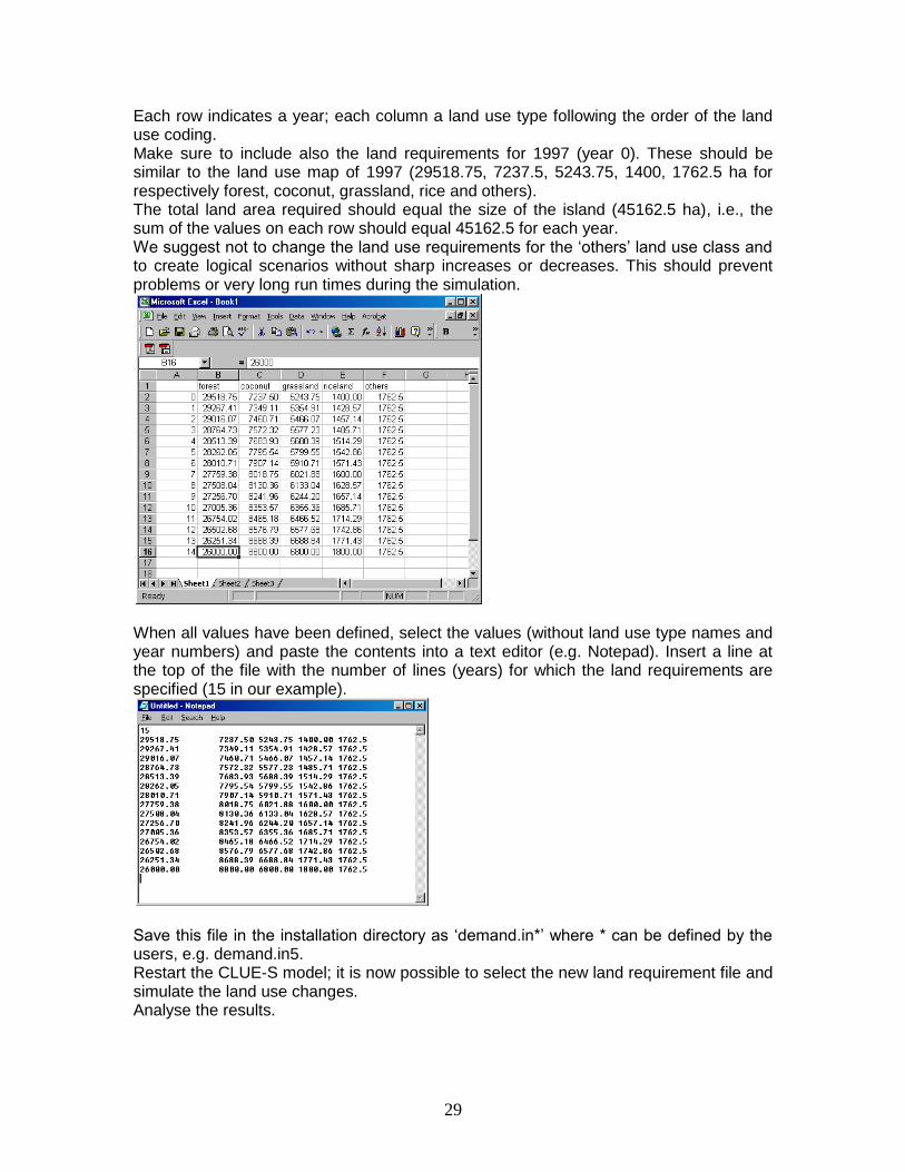
When all values have been defined, select the values (without land use type names and year numbers) and paste the contents into a text editor (e.g. Notepad). Insert a line at the top of the file with the number of lines (years) for which the land requirements are specified (15 in our example).

Save this file in the installation directory as ‘demand.in*’ where * can be defined by the users, e.g. demand.in5. Restart the CLUE-S model; it is now possible to select the new land requirement file and simulate the land use changes. Analyse the results.

30

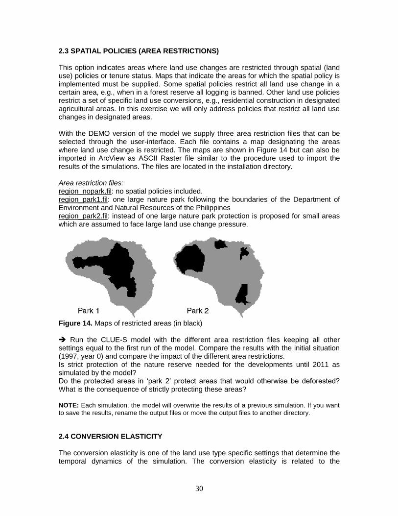
2.3 SPATIAL POLICIES (AREA RESTRICTIONS) This option indicates areas where land use changes are restricted through spatial (land use) policies or tenure status. Maps that indicate the areas for which the spatial policy is implemented must be supplied. Some spatial policies restrict all land use change in a certain area, e.g., when in a forest reserve all logging is banned. Other land use policies restrict a set of specific land use conversions, e.g., residential construction in designated agricultural areas. In this exercise we will only address policies that restrict all land use changes in designated areas. With the DEMO version of the model we supply three area restriction files that can be selected through the user-interface. Each file contains a map designating the areas where land use change is restricted. The maps are shown in Figure 14 but can also be imported in ArcView as ASCII Raster file similar to the procedure used to import the results of the simulations. The files are located in the installation directory. Area restriction files: region_nopark.fil: no spatial policies included. region_park1.fil: one large nature park following the boundaries of the Department of Environment and Natural Resources of the Philippines region_park2.fil: instead of one large nature park protection is proposed for small areas which are assumed to face large land use change pressure.

Figure 14. Maps of restricted areas (in black) Run the CLUE-S model with the different area restriction files keeping all other settings equal to the first run of the model. Compare the results with the initial situation (1997, year 0) and compare the impact of the different area restrictions. Is strict protection of the nature reserve needed for the developments until 2011 as simulated by the model? Do the protected areas in ‘park 2’ protect areas that would otherwise be deforested? What is the consequence of strictly protecting these areas? NOTE: Each simulation, the model will overwrite the results of a previous simulation. If you want to save the results, rename the output files or move the output files to another directory.

2.4 CONVERSION ELASTICITY The conversion elasticity is one of the land use type specific settings that determine the temporal dynamics of the simulation. The conversion elasticity is related to the

31

reversibility of land use changes. Land use types with high capital investment or irreversible impact on the environment will not easily be converted in other uses as long as there are land requirements for those land use types. Such land use types are therefore more ‘static’ than other land use types. Examples of relatively static land use types are residential areas, but also plantations with permanent crops (e.g., fruit trees). Other land use types are more easily converted when the location becomes more suitable for other land use types. Arable land often makes place for urban development while expansion of agricultural land can occur at the same time at the forest frontier. An extreme example is shifting cultivation: for this land use system the same location is mostly not used for periods exceeding two seasons as a consequence of nutrient depletion of the soil. These differences in behaviour towards conversion of the different land use types can be approximated by the conversion costs. However, costs cannot represent all factors that influence the decisions towards conversion such as nutrient depletion, esthetical value etc. Therefore, in the model we have assigned each land use type a dimensionless factor that represents the relative elasticity to conversion, ranging from 0 (easy conversion) to 1 (irreversible change). The user should specify this factor based on expert knowledge or observed behaviour in the recent past. An extended explanation of the possible values of the conversion elasticity and how behaviour changes when the land requirements increase or decrease in time is given below. 0: Means that all changes for that land use type are allowed, independent from

the current land use of a location. This means that a certain land use type can be removed at one place and allocated at another place at the same time, e.g. shifting cultivation.

>0...<1: Means that changes are allowed, however, the higher the value, the higher the preference that will be given to locations that are already under this land use type. This setting is relevant for land use types with high conversion costs.

1: Means that grid cells with one land use type can never be added and removed at the same time. This is relevant for land use types that are difficult to convert, e.g., urban settlements and primary forests. A value of one stabilizes the system and prevents that in case of deforestation other areas are reforested at the same time.

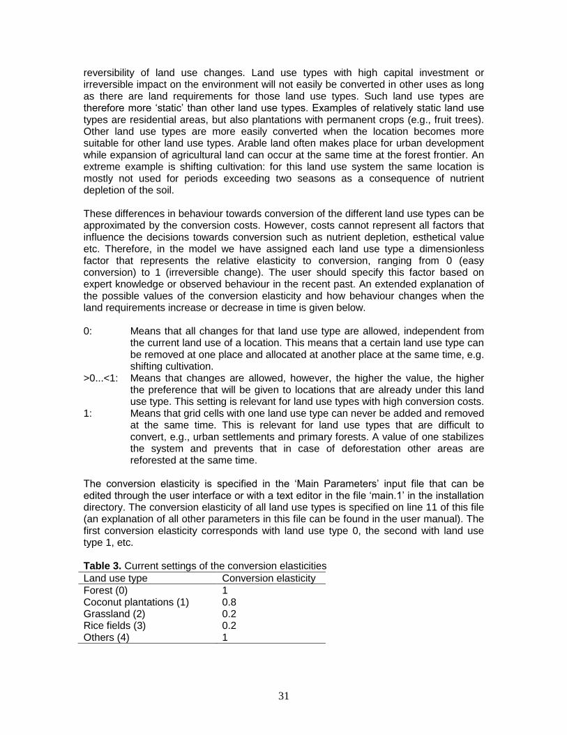
The conversion elasticity is specified in the ‘Main Parameters’ input file that can be edited through the user interface or with a text editor in the file ‘main.1’ in the installation directory. The conversion elasticity of all land use types is specified on line 11 of this file (an explanation of all other parameters in this file can be found in the user manual). The first conversion elasticity corresponds with land use type 0, the second with land use type 1, etc. Table 3. Current settings of the conversion elasticities

Land use type Conversion elasticity

Forest (0) Coconut plantations (1) Grassland (2) Rice fields (3) Others (4)

1 0.8 0.2 0.2 1

32

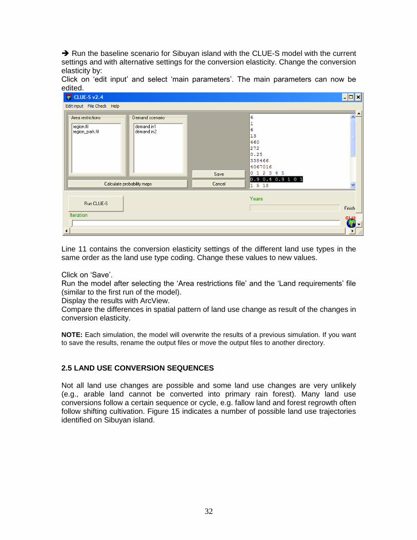
Run the baseline scenario for Sibuyan island with the CLUE-S model with the current settings and with alternative settings for the conversion elasticity. Change the conversion elasticity by: Click on ‘edit input’ and select ‘main parameters’. The main parameters can now be edited.

Line 11 contains the conversion elasticity settings of the different land use types in the same order as the land use type coding. Change these values to new values. Click on ‘Save’. Run the model after selecting the ‘Area restrictions file’ and the ‘Land requirements’ file (similar to the first run of the model). Display the results with ArcView. Compare the differences in spatial pattern of land use change as result of the changes in conversion elasticity. NOTE: Each simulation, the model will overwrite the results of a previous simulation. If you want to save the results, rename the output files or move the output files to another directory.

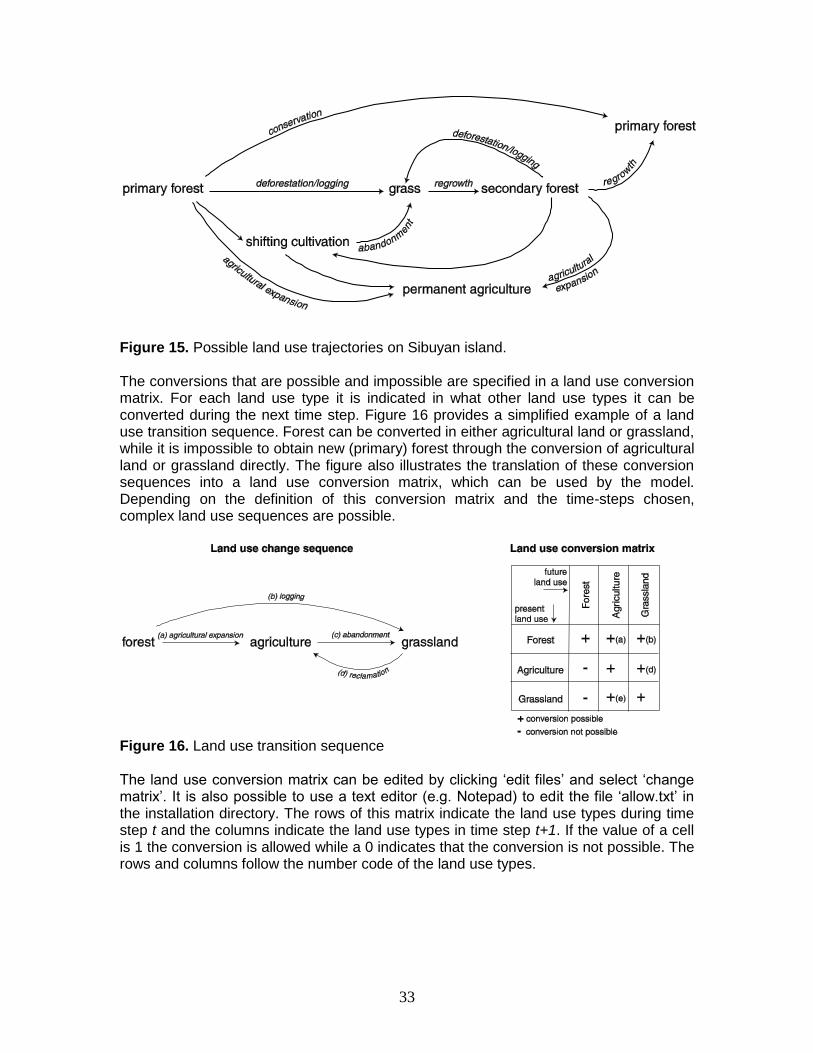
2.5 LAND USE CONVERSION SEQUENCES Not all land use changes are possible and some land use changes are very unlikely (e.g., arable land cannot be converted into primary rain forest). Many land use conversions follow a certain sequence or cycle, e.g. fallow land and forest regrowth often follow shifting cultivation. Figure 15 indicates a number of possible land use trajectories identified on Sibuyan island.

33

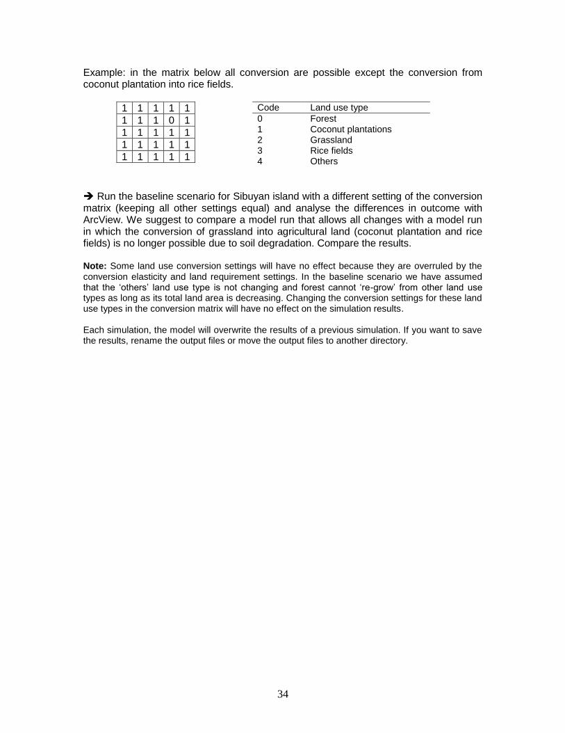
Figure 15. Possible land use trajectories on Sibuyan island. The conversions that are possible and impossible are specified in a land use conversion matrix. For each land use type it is indicated in what other land use types it can be converted during the next time step. Figure 16 provides a simplified example of a land use transition sequence. Forest can be converted in either agricultural land or grassland, while it is impossible to obtain new (primary) forest through the conversion of agricultural land or grassland directly. The figure also illustrates the translation of these conversion sequences into a land use conversion matrix, which can be used by the model. Depending on the definition of this conversion matrix and the time-steps chosen, complex land use sequences are possible.

Figure 16. Land use transition sequence The land use conversion matrix can be edited by clicking ‘edit files’ and select ‘change matrix’. It is also possible to use a text editor (e.g. Notepad) to edit the file ‘allow.txt’ in the installation directory. The rows of this matrix indicate the land use types during time step t and the columns indicate the land use types in time step t+1. If the value of a cell is 1 the conversion is allowed while a 0 indicates that the conversion is not possible. The rows and columns follow the number code of the land use types.

34

Example: in the matrix below all conversion are possible except the conversion from coconut plantation into rice fields.

1 1 1 1 1

1 1 1 0 1

1 1 1 1 1

1 1 1 1 1

1 1 1 1 1

Code Land use type

0 Forest 1 Coconut plantations 2 Grassland 3 Rice fields 4 Others

Run the baseline scenario for Sibuyan island with a different setting of the conversion matrix (keeping all other settings equal) and analyse the differences in outcome with ArcView. We suggest to compare a model run that allows all changes with a model run in which the conversion of grassland into agricultural land (coconut plantation and rice fields) is no longer possible due to soil degradation. Compare the results. Note: Some land use conversion settings will have no effect because they are overruled by the conversion elasticity and land requirement settings. In the baseline scenario we have assumed that the ‘others’ land use type is not changing and forest cannot ‘re-grow’ from other land use types as long as its total land area is decreasing. Changing the conversion settings for these land use types in the conversion matrix will have no effect on the simulation results. Each simulation, the model will overwrite the results of a previous simulation. If you want to save the results, rename the output files or move the output files to another directory.

35

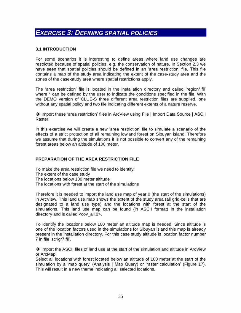
EXERCISE 3: DEFINING SPATIAL POLICIES 3.1 INTRODUCTION For some scenarios it is interesting to define areas where land use changes are restricted because of spatial policies, e.g. the conservation of nature. In Section 2.3 we have seen that spatial policies should be defined in an ‘area restriction’ file. This file contains a map of the study area indicating the extent of the case-study area and the zones of the case-study area where spatial restrictions apply. The ‘area restriction’ file is located in the installation directory and called ‘region*.fil’ where * can be defined by the user to indicate the conditions specified in the file. With the DEMO version of CLUE-S three different area restriction files are supplied, one without any spatial policy and two file indicating different extents of a nature reserve. Import these ‘area restriction’ files in ArcView using File | Import Data Source | ASCII Raster. In this exercise we will create a new ‘area restriction’ file to simulate a scenario of the effects of a strict protection of all remaining lowland forest on Sibuyan island. Therefore we assume that during the simulations it is not possible to convert any of the remaining forest areas below an altitude of 100 meter. PREPARATION OF THE AREA RESTRICTION FILE To make the area restriction file we need to identify: The extent of the case study The locations below 100 meter altitude The locations with forest at the start of the simulations Therefore it is needed to import the land use map of year 0 (the start of the simulations) in ArcView. This land use map shows the extent of the study area (all grid-cells that are designated to a land use type) and the locations with forest at the start of the simulations. This land use map can be found (in ASCII format) in the installation directory and is called <cov_all.0>. To identify the locations below 100 meter an altitude map is needed. Since altitude is one of the location factors used in the simulations for Sibuyan island this map is already present in the installation directory. For this case study altitude is location factor number 7 in file ‘sc1gr7.fil’. Import the ASCII files of land use at the start of the simulation and altitude in ArcView or ArcMap. Select all locations with forest located below an altitude of 100 meter at the start of the simulation by a ‘map query’ (Analysis | Map Query) or ‘raster calculation’ (Figure 17). This will result in a new theme indicating all selected locations.

36

Figure 17. Map query with ArcView In the ‘area restriction’ file the following coding should be used: 0: all grid cells that belong to the study area outside the ‘restricted area’ -9998: all grid cells for which land use conversions are not allowed during the simulations (the ‘restricted area’) ‘No Data’ or -9999: all other grid cells (outside the simulation area) Prepare an ‘area restriction’ file. You can follow the steps below or use your own procedure: Classify the land use map of year 0 to identify all cells inside the case study area (reclassify all land use types to 0; Analysis | Reclassify). Overlay the result with the forest areas below 100 meter. This can be done by the Map Calculator (Analysis | Map Calculator). The result only needs to be reclassified to the coding system of the area restriction file, as listed above (Analysis | Reclassify). Save this theme as a grid (Theme | Save Data Set). Export this theme as an ASCII file (File | Export Data Source) into the installation directory with a name following ‘region*.fil’ (where * can be defined by the user).

37

SIMULATE LAND USE CHANGE If you restart the CLUE-S model the new area restriction file should appear in the list of area restriction files and can be selected for the simulations. Run the model with the new area restriction file and compare the result with a simulation without protection of forest resources. Prepare your own area restriction file based on a hypothetical spatial policy. You can also prepare area restriction files by delineating areas in ArcView that need to be converted to grid cells. Note: If the area restrictions violate the land requirements specified in the ‘land requirements’ file the model will not succeed in allocating land use changes and stop the simulation. This can occur when all forest is assumed to be protected while at the same time a decrease in land requirements for forest is specified.

38

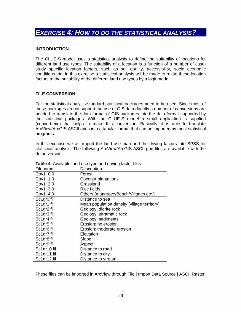
EXERCISE 4: HOW TO DO THE STATISTICAL ANALYSIS? INTRODUCTION The CLUE-S model uses a statistical analysis to define the suitability of locations for different land use types. The suitability of a location is a function of a number of case-study specific location factors, such as soil quality, accessibility, socio economic conditions etc. In this exercise a statistical analysis will be made to relate these location factors to the suitability of the different land use types by a logit model. FILE CONVERSION For the statistical analysis standard statistical packages need to be used. Since most of these packages do not support the use of GIS data directly a number of conversions are needed to translate the data format of GIS packages into the data format supported by the statistical packages. With the CLUE-S model a small application is supplied (convert.exe) that helps to make this conversion. Basically, it is able to translate ArcView/ArcGIS ASCII grids into a tabular format that can be imported by most statistical programs. In this exercise we will import the land use map and the driving factors into SPSS for statistical analysis. The following ArcView/ArcGIS ASCII grid files are available with the demo version: Table 4. Available land use type and driving factor files

Filename Description

Cov1_0.0 Cov1_1.0 Cov1_2.0 Cov1_3.0 Cov1_4.0

Forest Coconut plantations Grassland Rice fields Others (mangrove/Beach/Villages etc.)

Sc1gr0.fil Sc1gr1.fil Sc1gr2.fil Sc1gr3.fil Sc1gr4.fil Sc1gr5.fil Sc1gr6.fil Sc1gr7.fil Sc1gr8.fil Sc1gr9.fil Sc1gr10.fil Sc1gr11.fil Sc1gr12.fil

Distance to sea Mean population density (village territory) Geology: diorite rock Geology: ultramafic rock Geology: sediments Erosion: no erosion Erosion: moderate erosion Elevation Slope Aspect Distance to road Distance to city Distance to stream

These files can be imported in ArcView through File | Import Data Source | ASCII Raster.

39

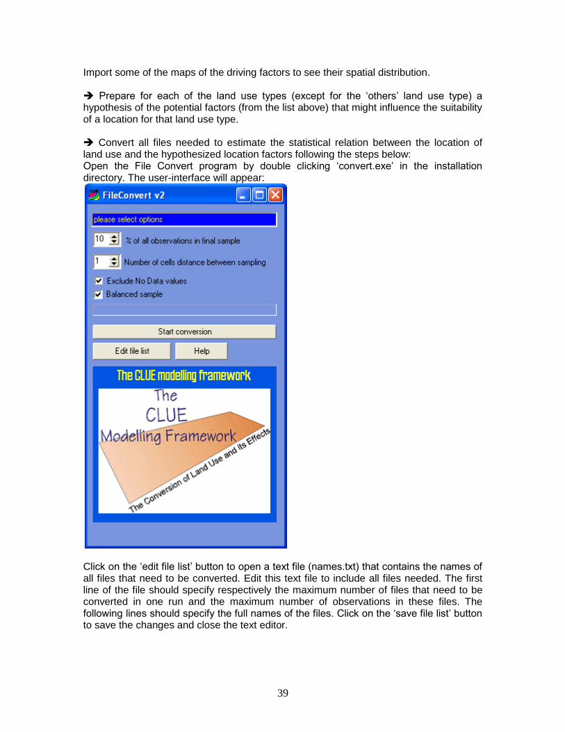
Import some of the maps of the driving factors to see their spatial distribution. Prepare for each of the land use types (except for the ‘others’ land use type) a hypothesis of the potential factors (from the list above) that might influence the suitability of a location for that land use type. Convert all files needed to estimate the statistical relation between the location of land use and the hypothesized location factors following the steps below: Open the File Convert program by double clicking ‘convert.exe’ in the installation directory. The user-interface will appear:

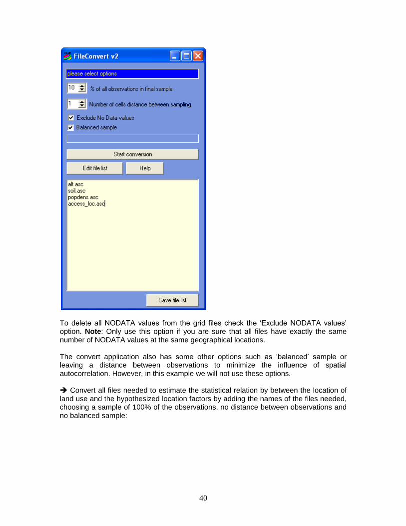
Click on the ‘edit file list’ button to open a text file (names.txt) that contains the names of all files that need to be converted. Edit this text file to include all files needed. The first line of the file should specify respectively the maximum number of files that need to be converted in one run and the maximum number of observations in these files. The following lines should specify the full names of the files. Click on the ‘save file list’ button to save the changes and close the text editor.

40

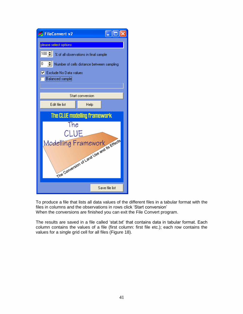
To delete all NODATA values from the grid files check the ‘Exclude NODATA values’ option. Note: Only use this option if you are sure that all files have exactly the same number of NODATA values at the same geographical locations. The convert application also has some other options such as ‘balanced’ sample or leaving a distance between observations to minimize the influence of spatial autocorrelation. However, in this example we will not use these options. Convert all files needed to estimate the statistical relation by between the location of land use and the hypothesized location factors by adding the names of the files needed, choosing a sample of 100% of the observations, no distance between observations and no balanced sample:

41

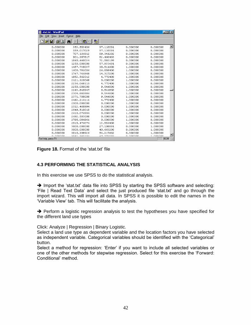
To produce a file that lists all data values of the different files in a tabular format with the files in columns and the observations in rows click ‘Start conversion’ When the conversions are finished you can exit the File Convert program. The results are saved in a file called ‘stat.txt’ that contains data in tabular format. Each column contains the values of a file (first column: first file etc.); each row contains the values for a single grid cell for all files (Figure 18).

42

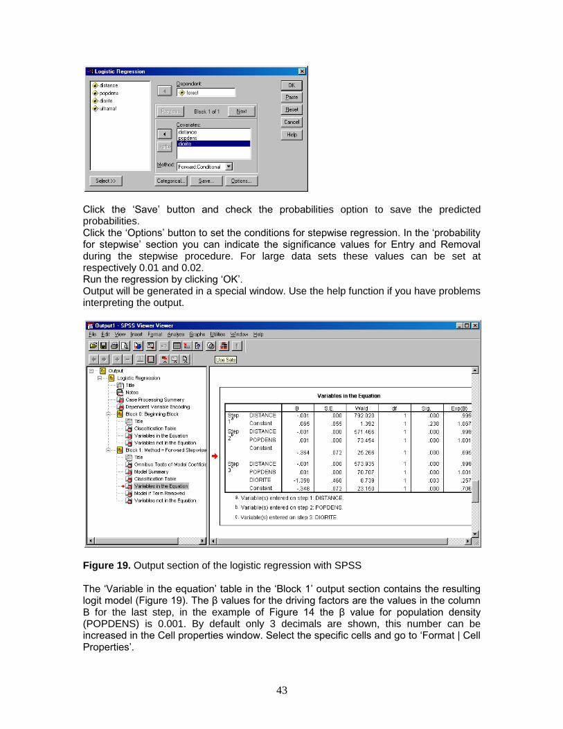
Figure 18. Format of the ‘stat.txt’ file 4.3 PERFORMING THE STATISTICAL ANALYSIS In this exercise we use SPSS to do the statistical analysis. Import the ‘stat.txt’ data file into SPSS by starting the SPSS software and selecting: ‘File | Read Text Data’ and select the just produced file ‘stat.txt’ and go through the import wizard. This will import all data. In SPSS it is possible to edit the names in the ‘Variable View’ tab. This will facilitate the analysis. Perform a logistic regression analysis to test the hypotheses you have specified for the different land use types Click: Analyze | Regression | Binary Logistic. Select a land use type as dependent variable and the location factors you have selected as independent variable. Categorical variables should be identified with the ‘Categorical’ button. Select a method for regression: ‘Enter’ if you want to include all selected variables or one of the other methods for stepwise regression. Select for this exercise the ‘Forward: Conditional’ method.

43

Click the ‘Save’ button and check the probabilities option to save the predicted probabilities. Click the ‘Options’ button to set the conditions for stepwise regression. In the ‘probability for stepwise’ section you can indicate the significance values for Entry and Removal during the stepwise procedure. For large data sets these values can be set at respectively 0.01 and 0.02. Run the regression by clicking ‘OK’. Output will be generated in a special window. Use the help function if you have problems interpreting the output.

Figure 19. Output section of the logistic regression with SPSS The ‘Variable in the equation’ table in the ‘Block 1’ output section contains the resulting logit model (Figure 19). The β values for the driving factors are the values in the column B for the last step, in the example of Figure 14 the β value for population density (POPDENS) is 0.001. By default only 3 decimals are shown, this number can be increased in the Cell properties window. Select the specific cells and go to ‘Format | Cell Properties’.

44

45

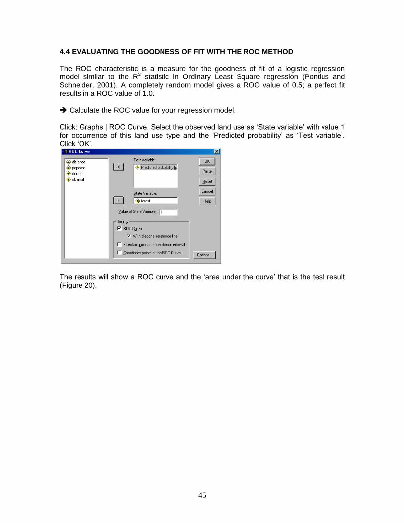
4.4 EVALUATING THE GOODNESS OF FIT WITH THE ROC METHOD The ROC characteristic is a measure for the goodness of fit of a logistic regression model similar to the R2 statistic in Ordinary Least Square regression (Pontius and Schneider, 2001). A completely random model gives a ROC value of 0.5; a perfect fit results in a ROC value of 1.0. Calculate the ROC value for your regression model. Click: Graphs | ROC Curve. Select the observed land use as ‘State variable’ with value 1 for occurrence of this land use type and the ‘Predicted probability’ as ‘Test variable’. Click ‘OK’.

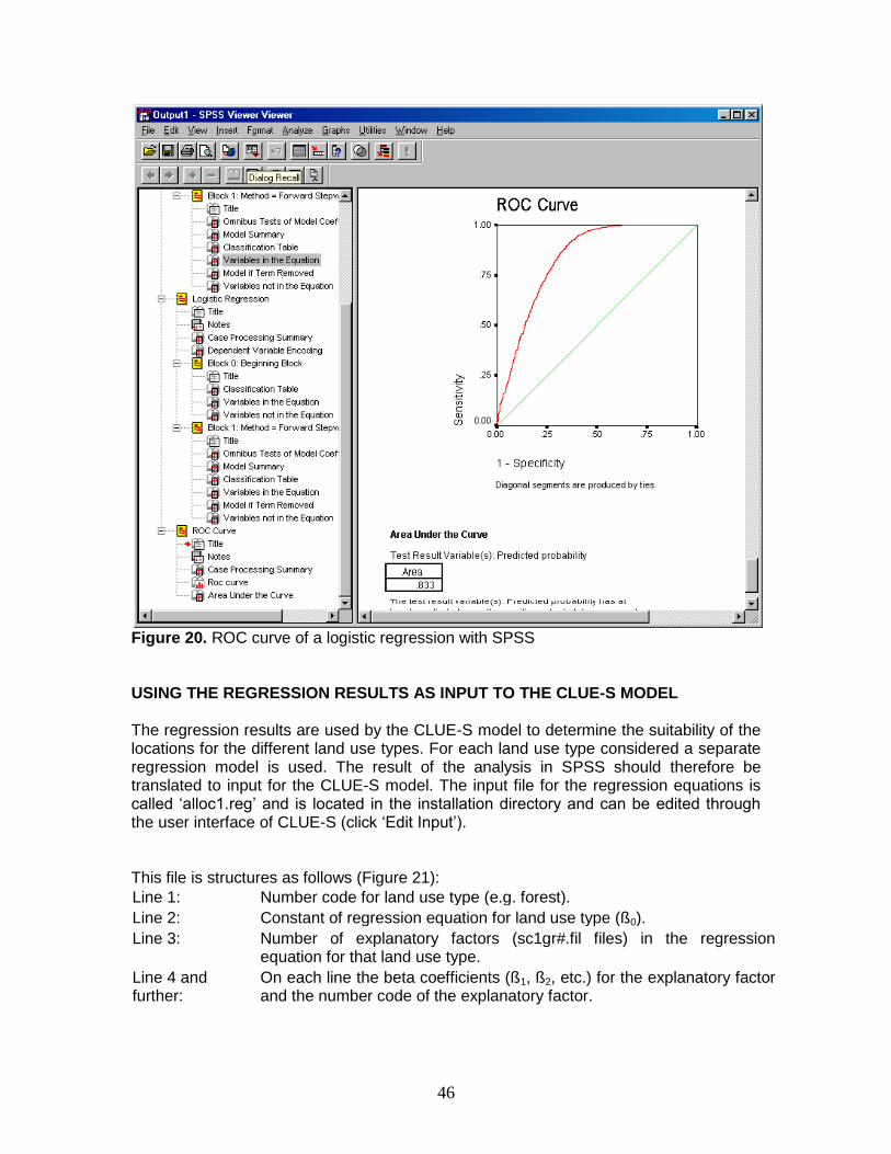
The results will show a ROC curve and the ‘area under the curve’ that is the test result (Figure 20).

46

Figure 20. ROC curve of a logistic regression with SPSS USING THE REGRESSION RESULTS AS INPUT TO THE CLUE-S MODEL The regression results are used by the CLUE-S model to determine the suitability of the locations for the different land use types. For each land use type considered a separate regression model is used. The result of the analysis in SPSS should therefore be translated to input for the CLUE-S model. The input file for the regression equations is called ‘alloc1.reg’ and is located in the installation directory and can be edited through the user interface of CLUE-S (click ‘Edit Input’). This file is structures as follows (Figure 21):

Line 1: Number code for land use type (e.g. forest).

Line 2: Constant of regression equation for land use type (ß0).

Line 3: Number of explanatory factors (sc1gr#.fil files) in the regression equation for that land use type.

Line 4 and further:

On each line the beta coefficients (ß1, ß2, etc.) for the explanatory factor and the number code of the explanatory factor.

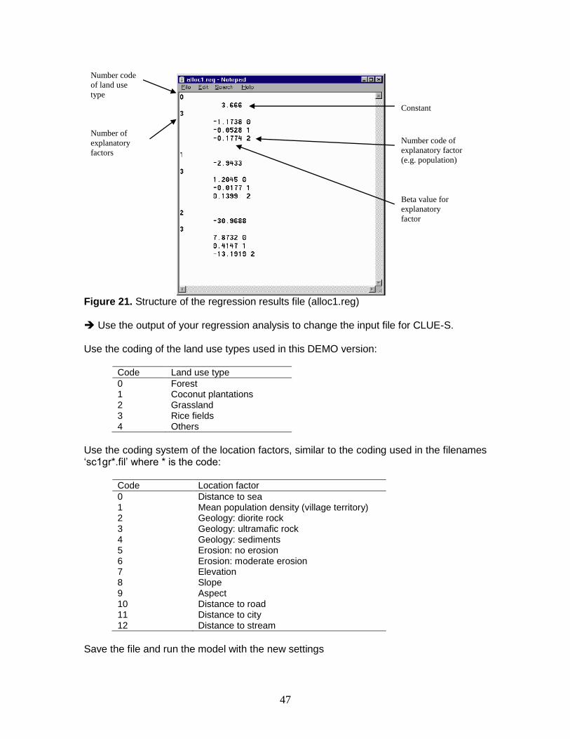
47

Figure 21. Structure of the regression results file (alloc1.reg) Use the output of your regression analysis to change the input file for CLUE-S. Use the coding of the land use types used in this DEMO version:

Code Land use type

0 Forest 1 Coconut plantations 2 Grassland 3 Rice fields 4 Others

Use the coding system of the location factors, similar to the coding used in the filenames ‘sc1gr*.fil’ where * is the code:

Code Location factor

0 1 2 3 4 5 6 7 8 9 10 11 12

Distance to sea Mean population density (village territory) Geology: diorite rock Geology: ultramafic rock Geology: sediments Erosion: no erosion Erosion: moderate erosion Elevation Slope Aspect Distance to road Distance to city Distance to stream

Save the file and run the model with the new settings

Number code

of land use

type

Number of

explanatory

factors

Constant

Number code of

explanatory factor

(e.g. population)

Beta value for

explanatory

factor

48

Compare the results of simulations with different location factors included in the regression analysis. Probability maps solely based on the regression equations can be generated with the ‘Calculate probability maps’ button in CLUE-S and are stored in ‘prob1_*.1’ where * indicates the land use code. These maps can be imported as floating point grids in ArcView ‘File | Import Data Source | ASCII Raster’. Note: do not import as integers. Do different regressions result in different probability maps? Do different probability maps result in different simulation results of the land use change model?

49

Exercise 5: Simulating a new scenario of land use change for Sibuyan Island Create a storyline for the development of Sibuyan island for the next 20 years. The storyline should take into account developments for which the analysis might provide relevant information for the provincial government. The provincial government has the power to stimulate certain land use reform programs, nature protection or improve the control on illegal logging. Translate this storyline into a model scenario that can be run by the CLUE model by varying the demand, area restrictions, conversion matrix and the land use type elasticity. Run your scenario and analyze the outcome. Prepare 1 map, table, diagram or graph based on your results that shows your most important message to the policy makers.

QUESTION 1 Prepare a short presentation that includes: -your storyline

-the main ‘message’ you would like to give to the policy makers presented in such a way

that the result is clear to policy makers that are not interested in land use modeling itself.

50

EXERCISE 6: CREATING YOUR OWN DYNA-CLUE APPLICATION: A STEPWISE PROCEDURE Step 1: Is Dyna-CLUE the adequate tool for my research questions? The exercises, paper and descriptions of the CLUE models should have given you a good idea of what you can use the model for. Basically, the CLUE modelling framework is developed to spatially allocate land use changes for visualising the impacts of different scenarios on land use patterns. In case your research has different objectives, e.g., determining the aggregate quantity of land use change as result of economic policies, it is better to choose another model. Step 2: Do you have sufficient information with respect to changes in demand for land use areas at the aggregate level? The Dyna-CLUE model requires projections of the change in area for the different land cover types at the level of the study region as a whole. These may be derived from trend extrapolation (so trends are needed), from rough scenario assumptions (e.g., a 10% increase of agricultural area over the next 20 years) or from advanced models such as global global economic models or integrated assessment models (as in www.eururalis.nl). For a specific application it may also be possible to combine methods for the different land cover types, as long as is made sure that the results are leading to a consistent change in land areas, i.e., equalling the total area available within the study region. These data should be prepared before the Dyna-CLUE modelling is started. Step 3: Build a conceptual model for your study area The conceptual model should address a number of questions relevant to the design of the model: Q1: What is the extent of the study area that you want to address? Q2: What are the land use types that you are interested in (only include land use types for which you think information is available)? Q3: List for each of the land use types a number of location factors which you think may affect allocation decisions? Q4: Determine for each of the land use types how you will determine the change in area at the level of the study region (see step 2) Q5: Are there any specific, fixed conversion trajectories that need to be taken into account? Q6: Are there specific spatial polices to be considered? The answers to these questions can be filled in the diagram (figure 1) for a schematized model setup Step 4: Prepare data

51

-Choose the resolution of your spatial data based on the resolution of your land use data and location factor data. It makes no sense to choose a resolution for which the location factors do not show any variation between cells. Furthermore, a high spatial resolution will result in high calculation times. Calculation times are reasonable at resolutions below 1200x1200 cells. -Convert all spatial data to a similar projection. Equal area projections are preferred -Reclassify thematic data to a classification to be used in the modelling, e.g., the land use types or the classes to be used as location factors. Please note that the first class should always have class number 0. -Convert all data to a grid with the same extent and resolution (pls note that the upper left corner of each grid should be located at exactly the same location) -Prepare a ‘mask’ that contains value 1 inside the study area and ‘nodata’ outside. -Fill gabs within all data layers, either by adding auxiliary data or by interpolation methods (e.g., ‘assign proximity’ / ‘eucallocate’). -Multiply all layers with the mask -Export all data to ASCII grid data files. It is easiest to directly use the naming conventions of CLUE: cov_all.0 for the initial land cover and sc1gr[number coding].fil for the location factors

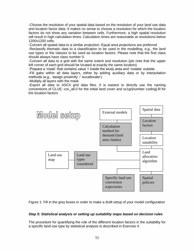
Figure 1: Fill in the grey boxes in order to make a draft setup of your model configuration Step 5: Statistical analysis or setting up suitability maps based on decision rules The procedure for quantifying the role of the different location factors in the suitability for a specific land use type by statistical analysis is described in Exercise 4.

External models

Specific land use

conversion

trajectories

Spatial

policies

Land use

types

considered

Land use

map

Land

allocation

algorithm

Calculation

method for

demand (land

area claims) Location

suitability

Location

factors

Spatial data

52

Step 6: Create a directory for your model application CLUE only needs and produces files within one directory. It is most convenient to create a new directory for your application and store all the files that you prepare for the model in that directory. You may start by copying clues.exe and clues.hlp into the directory. Note that if you use ArcView3.x it is not possible to have spaces within the path name (e.g. c:/documents and settings/clue). Step 7: Prepare demand / land area claim file The procedure is described in exercise 2.2. Please note that the total area of all land use types together may not change or exceed the surface area of the active cells within the study area. Indicate in the top line the total number of lines in this file, this should equal the number of years to be simulated plus the initial year. The second line of the file gives the surface area of the land use types in the initial year. This should equal the area as indicated in the map of the initial year (cov_all.0). Please note that the units should be equal to the units as specified in the main parameter file, if the reference units of all maps are in meters the preferred land area unit is hectares. The resulting demand file should be saved in the simulation directory with the name demand.in* with * being a number or character. Step 8: Prepare a region file In the standard region file all cells that have a land use type in the initial situation are allowed to change. This standard region file can easily be made by reclassifying the mask made in step 4 to value 0 in all cells that need to be calculated and ‘no data’/’-9999’ in all other cells. This file needs to be exported to an ASCII file and saved in the simulation directory as region**.fil where ** may be any name with multiple characters. For scenarios in which certain areas are not allowed to change it is possible to create an alternative region file in which the ‘static’ regions are assigned value -9998. Step 9: Copy all files with location factors in the simulation directory If you did not yet do so in step 4 it is now needed to copy all location factors used in the statistical models into the simulation directory as ASCII grid files named sc1gr*.fil where * stands for the location factor number. Note that numbering should be consecutive and start with 0. Step 10: Copy the initial land use map to the simulation directory This file should contain the initial land use map with land uses numbered consecutive from 0 onwards. The format is ASCII grid named cov_all.0 Step 11: Set-up the main parameter file

53

Create within the simulation directory a text file called main.1 (e.g. by opening Notepad and saving an empty text file). You can now edit this file using the CLUE interface (click clues.exe / file | edit main parameters) or by editing the main.1 file with a text editor (Notepad/Wordpad etc.). In the CLUE-help file you can exactly read what parameters need to be defined. Define all parameter settings as adequate for your case study area. Step 12: Create the regression parameter file Create within the simulation directory a text file called alloc1.reg (e.g. by opening Notepad and saving an empty text file). You can now edit this file using the CLUE interface (click clues.exe / file | edit regression results) or by editing the alloc1.reg file with a text editor (Notepad/Wordpad etc.). In the CLUE-help file you can exactly read how the file should be formatted. The file should reflect the results of the statistical analysis. In case for one land use type no changes in land use are simulated (e.g., a static land use type) it is still needed to define parameters for the regression equation. In that case a regression with equal values should be indicates, e.g., a constant with value 0.7 and 1 location factor with beta value 0. Step 13: Create the conversion matrix Create within the simulation directory a text file called allow.txt (e.g. by opening Notepad and saving an empty text file). You can now edit this file using the CLUE interface (click clues.exe / file | edit conversion matrix) or by editing the allow.txt file with a text editor (Notepad/Wordpad etc.). In the CLUE-help file you can exactly read how the file should be formatted. It is easiest to first conceptually think which conversions are possible and which are not possible. This can be implemented by the values 1 and 0 in the conversion matrix. After a test run is successfully made it is possible to further specify the matrix with time lags and other more advanced options. Step 14: Optional: specify neighbourhood interactions See the help file for more information. In case neighbourhood interactions are not considered (option 0 for neighbourhood interactions in the main parameter file) these files do not need to be specified. Step 15: Test the model Start the model by selecting a demand file, region file and click RUN!