BMeteorologische Zeitschrift, Vol. 26, No. 2, 115–125 (published online January 24, 2017) Climatology© 2016 The authors

The climate of the European Alps: Shift of very highresolution Köppen-Geiger climate zones 1800–2100

Franz Rubel1∗, Katharina Brugger1, Klaus Haslinger2 and Ingeborg Auer2

1Institute for Veterinary Public Health, University of Veterinary Medicine Vienna, Austria2Central Institute for Meteorology and Geophysics, Vienna, Austria

(Manuscript received July 25, 2016; in revised form September 8, 2016; accepted October 4, 2016)

AbstractAlthough the European Alps are one of the most investigated regions worldwide, maps depicting climatechange by means of climate classification are still not-existent. To contribute to this topic, a time seriesof very high resolution (30 arc-seconds) maps of the well-known Köppen-Geiger climate classificationis presented. The maps cover the greater Alpine region located within the geographical domain of 4to 19 degrees longitude and 43 to 49 degrees latitude. Gridded monthly data were selected to compileclimate maps within this region. Observations for the period 1800–2010 were taken from the historicalinstrumental climatological surface time series of the greater Alpine region, HISTALP. Projected climatedata for the period 2011–2100 were taken, as an example, from the Rossby Centre regional atmosphericmodel RCA4. Temperature fields were spatially disaggregated by applying the observed seasonal cycle ofthe environmental lapse rate. The main results of this study are, therefore, 366 observed and predicted (twoscenarios) very high resolution Köppen-Geiger climate maps of the greater Alpine region covering the period1800–2100. Digital data, as well as animated maps, showing the shift of the climate zones are provided on thefollowing website http://koeppen-geiger.vu-wien.ac.at. Furthermore, the relationship between the Köppen-Geiger climate classification and the altitudinal belts of the Alps is demonstrated by calculating the boundariesof the climate zones, i.e. the deciduous forest line, the mixed forest line, the forest and tree line (timber line)and the snow line. The mean altitude of the potential timber line in the greater Alpine region, for example,was calculated to be 1730 m by the end of the 19th century, 1880 m by the end of the 20th century and to liebetween 2120 and 2820 m by the end of the 21st century. The latter altitudes were projected for the greenhousegas scenarios RCP 2.6 (best case) and RCP 8.5 (worst case). The altitude of the timber line (and the otherboundaries of the altitudinal belts) is generally higher in the Western Alps, showing a clear west-east slope.

Keywords: HISTALP, COSMO-CLM, representative concentration pathways, altitudinal belts, timber line

1 Introduction

The European Alps are one of the most investigatedregions worldwide with respect to climate, climatechange and the impacts of climate change. Examplesof this includes a report of precipitation climatologypresented by Frei and Schär (1998) and mapped bySchwarb et al. (2000), temperature trends investigatedby Böhm et al. (2001) and the recent modelling study ofHaslinger et al. (2016) which addressed future droughtprobabilities. Of general interest is the alpine vegeta-tion which is particularly sensitive to the effects ofclimate change (Grabherr et al., 1994; Theurillatand Guisan, 2001). Spatio-temporal analysis of altitu-dinal vegetation shifts, for example, was investigatedby Diaz-Varela et al. (2007), while Gottfried et al.(2011) demonstrated the coincidence of the alpine-nivalecotone with the summer snow line. The winter snowline varies considerably under the influence of European

∗Corresponding author: Franz Rubel, Climate Change and Infectious Dis-eases Group, Institute for Veterinary Public Health, University of Vet-erinary Medicine Vienna, 1210 Vienna, Austria, e-mail: franz.rubel@vetmeduni.ac.at

temperature fluctuations (Hantel and Hirtl-Wielke,2007), is located at an average altitude of 640 m andis characterized by an upward shift of approximately120 m per °C climate warming (Hantel and Maurer,2011).

Independent of these specific examinations, the sci-entific community requires a simple method to describethe climate or climate change of a specified region. Forthis purpose, the Köppen-Geiger climate classificationin particular has proved successful. The generic climateclassification initially developed by Wladimir Köppen(1846–1940) and Rudolf Geiger (1894–1981) was pre-sented in its most popular version by Köppen (1936) andhas today been established as a multidisciplinary stan-dard to characterize the climate of a region (Rubel andKottek, 2011). Applications of the Köppen-Geiger cli-mate classification include investigations on: (1) the sub-division of study sites according to climates such as formicrometeorological flux measurements (Mizoguchiet al., 2009) or for global river discharge (Santini anddi Paola, 2015), (2) the extraction of climate zonesto assess vegetation coverage and biomass of temper-ate deserts (Zhang et al., 2016a) or the definition of the

© 2016 The authorsDOI 10.1127/metz/2016/0816 Gebrüder Borntraeger Science Publishers, Stuttgart, www.borntraeger-cramer.com

116 F. Rubel et al.: The climate of the European Alps Meteorol. Z., 26, 2017

Mediterranean region to review post-wildfire soil ero-sion (Shakesby, 2011), (3) the effect on human thermalcomfort by urban street configurations (Rodríguez Al-geciras et al., 2016), (4) the effect of particulate air pol-lution on human mortality in the USA (Zanobetti andSchwartz, 2009), (5) the composition of disease vec-tors in Europe (Brugger and Rubel, 2013), (6) thehabitat characterization of new species in South Amer-ica (Bellini and Zeppelini, 2008), and numerous otherstudies.

While historical world maps of Köppen-Geiger cli-mate classification were exclusively available as handdrawn maps, e.g. in its latest version from Geiger(1961), early digital world maps were compiled to ver-ify global climate models (Manabe and Holloway,1975) and to depict the observed shift of climate zones(Fraedrich et al., 2001). The first digital dataset cover-ing the observational period 1951–2000 was publishedby Kottek et al. (2006). This dataset is publicly avail-able via the website http://koeppen-geiger.vu-wien.ac.at/ and paved the way for easy access to climate classifi-cation in various research fields. Four years later Rubeland Kottek (2010) published a time series of Köppen-Geiger maps depicting the shift of climate zones overthe 200-year period 1901–2100. These maps were cal-culated from monthly temperature fields provided by theClimatic Research Unit (CRU) of the University of EastAnglia (Mitchell and Jones, 2005) and precipitationfields provided by the Global Precipitation ClimatologyCentre (Becker et al., 2013; Schneider et al., 2014)as well as from an ensemble of global climate modelpredictions. Recently, various authors published simi-lar Köppen-Geiger maps based on model outputs cal-culated for the Climate Model Intercomparison Project(CMIP) and the Paleo Model Intercomparison Project(PMIP). CMIP maps were presented and discussed, forexample, by Feng et al. (2014), PMIP maps by Yoo andRohli (2016) and Zhang et al. (2016b), while Willmeset al. (2016) developed an open source software to cal-culate Köppen-Geiger maps from the databases of bothprojects.

Global climate classifications have also been ap-plied to continental and regional scales, thereby gener-ating valuable information in particular for life sciences.Köppen-Geiger maps, for example, have been publishedfor Australia (Crosbie et al., 2012), Brazil (Alvareset al., 2013), South Africa (Engelbrecht and Engel-brecht, 2014) and China (Chan et al., 2016).

Here, the concept of climate classification is appliedto the greater Alpine region to depict the shift of cli-mate zones during the 301-year period 1800–2100. Spe-cial emphasis is placed on the spatial resolution of thedigital maps which were not only provided as picturesbut also as digital data. The latter were urgently re-quired for many scientific applications. At present, re-searchers may use either digital data available with aspatial resolution of 0.5 degrees or less as provided bythe studies discussed above or can calculate their ownKöppen-Geiger maps from very high resolution tem-

perature and precipitation fields provided by Hijmanset al. (2005). The latter data are representative for theperiod 1950–2000 and are provided with a spatial reso-lution of 30′′ (30 arc-seconds). The goal of this paper isto use the well-documented HISTALP database (Aueret al., 2007), as well as model predictions from EURO-CORDEX (Jacob et al., 2014), both spatially disag-gregated, to compile a series of Köppen-Geiger maps.These maps have the same spatial resolution of 30′′

than those of Hijmans et al. (2005), but have been cal-culated as a 25-year running mean from homogenizedtime series covering the period 1800–2010 and state-of-the-art regional climate model predictions for the years2011–2100.

2 Data and method

The greater Alpine region is defined as being locatedbetween 4° and 19° geographic longitude and 43° to49° geographic latitude. Three gridded climate datasetswere selected to calculate very high resolution Köppen-Geiger climate maps within this region. The first dataset,the historical instrumental climatological surface timeseries of the greater Alpine region, HISTALP (Aueret al., 2007), comprised temperature fields for the pe-riod 1780–2008 and precipitation fields for the pe-riod 1800–2010 (http://www.zamg.ac.at/histalp/). Forthis study, the temperature fields were extended un-til 2010 with the aim of achieving the joint observa-tional period 1800–2010. Monthly HISTALP tempera-ture fields (Böhm et al., 2001; Chimani et al., 2013) andprecipitation fields (Efthymiadis et al., 2006; Chimaniet al., 2011) were available on a grid equidistant in ge-ographic latitude and longitude with a spatial resolu-tion of 5′ (around 6.5 km · 9.3 km � 60 km2). The sec-ond dataset, monthly precipitation analyses from Isottaet al. (2014, 2015) based on 5,500 daily rain gauge ob-servations, is used as a reference for the high spatialvariability of Alpine precipitation. These precipitationfields cover the major part of the greater Alpine regionand were nested into the HISTALP precipitation fieldsfor the reference period 1986–2010. From the latter ob-served and projected precipitation anomalies were cal-culated and used as input data for the Köppen-Geigermaps. This procedure considers the high spatial reliabil-ity of the reference fields from Isotta et al. (2014) byeliminating the spatial bias of the HISTALP precipita-tion fields, which were analysed from 557 homogenisedtime series.

The third dataset was taken from the EURO-COR-DEX ensemble (Jacob et al., 2014). It includes a va-riety of climate predictions from different global andregional climate model combinations, which were runfor the predefined greenhouse gas emission scenarios.As the main focus of this research lies on the ob-served shift of climate zones, only the two most ex-treme greenhouse gas concentrations for the represen-tative concentration pathways, RCP 2.6 and RCP 8.5

Meteorol. Z., 26, 2017 F. Rubel et al.: The climate of the European Alps 117

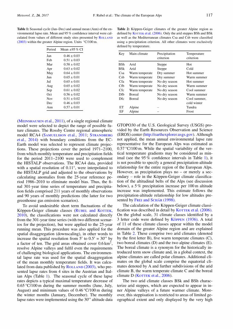
Table 1: Seasonal cycle (Jan–Dec) and annual mean (Ann) of the en-vironmental lapse rate. Mean and 95 % confidence interval were cal-culated from values of different study sites presented by Rolland(2003) within the greater Alpine region. Units °C/100 m.

Period Mean ±95 % CI

Jan 0.46 ± 0.03Feb 0.51 ± 0.03Mar 0.58 ± 0.02Apr 0.63 ± 0.02May 0.64 ± 0.01Jun 0.65 ± 0.01Jul 0.65 ± 0.01Aug 0.65 ± 0.02Sep 0.61 ± 0.02Oct 0.56 ± 0.02Nov 0.51 ± 0.02Dec 0.46 ± 0.03Ann 0.57 ± 0.01

(Meinshausen et al., 2011), of a single regional climatemodel were selected to depict the range of possible fu-ture climates. The Rossby Centre regional atmosphericmodel RCA4 (Samuelsson et al., 2011; Strandberget al., 2014) with boundary conditions from the EC-Earth model was selected to represent climate projec-tions. These projections cover the period 1971–2100,from which monthly temperature and precipitation fieldsfor the period 2011–2100 were used to complementthe HISTALP observations. The RCA4 data, providedwith a spatial resolution of 0.11°, were interpolated tothe HISTALP grid and adjusted to the observations bycalculating anomalies from the 25-year reference pe-riod 1986–2010 to eliminate model bias. Thus, the fi-nal 301-year time series of temperature and precipita-tion fields comprised 211 years of monthly observationsand 90 years of monthly predictions (the latter for twogreenhouse gas emission scenarios).

To avoid undesirable short term fluctuations of theKöppen-Geiger climate classes (Rubel and Kottek,2010), the classifications were not calculated directlyfrom the 301-year time series (with two different scenar-ios for the projection), but were applied to the 25-yearrunning mean. This procedure was also applied for thespatial disaggregation (downscaling), in other words toincrease the spatial resolution from 5′ to 0.5′ = 30′′ bya factor of ten. The grid areas obtained cover 0.6 km2,resolve Alpine valleys and fulfil even the requirementsof challenging biological applications. The environmen-tal lapse rate was used for the spatial disaggregationof the mean monthly temperature fields. It was calcu-lated from data published by Rolland (2003), who pre-sented lapse rates from 4 sites in the Austrian and Ital-ian Alps (Table 1). The seasonal cycle of these lapserates depicts a typical maximal temperature decrease of0.65 °C/100 m during the summer months (June, July,August) and minimum values of 0.46 °C/100 m duringthe winter months (January, December). The monthlylapse rates were implemented using the 30′′ altitude data

Table 2: Köppen-Geiger climates of the greater Alpine region asdefined by Kottek et al. (2006). Only the arid steppes BSh and BSkas well as the Mediterranean climates Csa and Csb were classifiedusing a precipitation criterion. All other climates were exclusivelydefined by temperature.

Key Main climate Precipitationcriterion

Temperaturecriterion

BSh Arid Steppe HotBSk Arid Steppe ColdCsa Warm temperate Dry summer Hot summerCsb Warm temperate Dry summer Warm summerCfa Warm temperate No dry season Hot summerCfb Warm temperate No dry season Warm summerCfc Warm temperate No dry season Cool summerDfb Boreal No dry season Warm summerDfc Boreal No dry season Cool summer,

cold winterET Alpine – TundraEF Alpine – Frost

GTOPO30 of the U.S. Geological Survey (USGS) pro-vided by the Earth Resources Observation and Science(EROS) center (http://earthexplorer.usgs.gov). Althoughnot applied, the mean annual environmental lapse raterepresentative for the European Alps was estimated as0.57 °C/100 m. While the spatial variability of the ver-tical temperature gradients may be considered as min-imal (see the 95 % confidence intervals in Table 1), itis not possible to specify a general precipitation-altituderelationship for the entire region of the European Alps.However, as precipitation plays no – or merely a sec-ondary – role in the Köppen-Geiger climate classifica-tion of the altitudinal belts of the Alps (see discussionbelow), a 5 % precipitation increase per 100 m altitudeincrease was implemented. This estimate follows theprecipitation-altitude relationship for low altitudes pre-sented by Frei and Schär (1998).

The calculation of the Köppen-Geiger climate classi-fication was described in detail by Kottek et al. (2006).On the global scale, 31 climate classes identified by a3 letter code were defined by Köppen (1936). A totalof 11 of these climate classes appear within the modeldomain of the greater Alpine region and are explainedin Table 2. These comprise two arid climates (denotedby the first letter B), five warm temperate climates (C),two boreal climates (D) and the two alpine climates (E).The boreal climate is a synonym for the historically in-troduced term snow climate and, in a global context, thealpine climates are called polar climates. Additional cli-mates on the global scale comprise the equatorial cli-mates denoted by A and further subdivisions of the aridclimate B, the warm temperate climate C and the borealclimate D (Kottek et al., 2006).

The two arid climate classes BSk and BSh charac-terize arid steppes, which are expected to appear in in-ner Alpine valleys of a future warmer climate. More-over, this steppisation is restricted to areas of limited ge-ographical extent and only displayed by the very high

118 F. Rubel et al.: The climate of the European Alps Meteorol. Z., 26, 2017

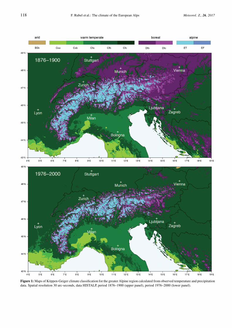
Figure 1: Maps of Köppen-Geiger climate classification for the greater Alpine region calculated from observed temperature and precipitationdata. Spatial resolution 30 arc-seconds, data HISTALP, period 1876–1900 (upper panel), period 1976–2000 (lower panel).

Meteorol. Z., 26, 2017 F. Rubel et al.: The climate of the European Alps 119

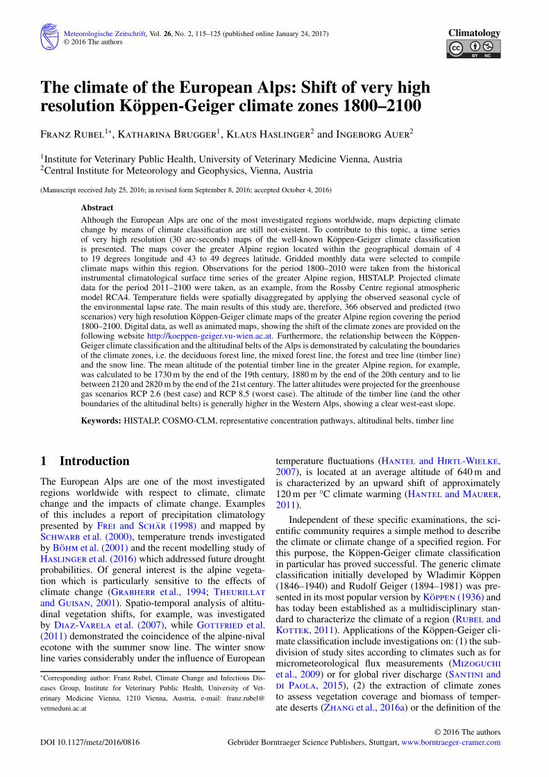
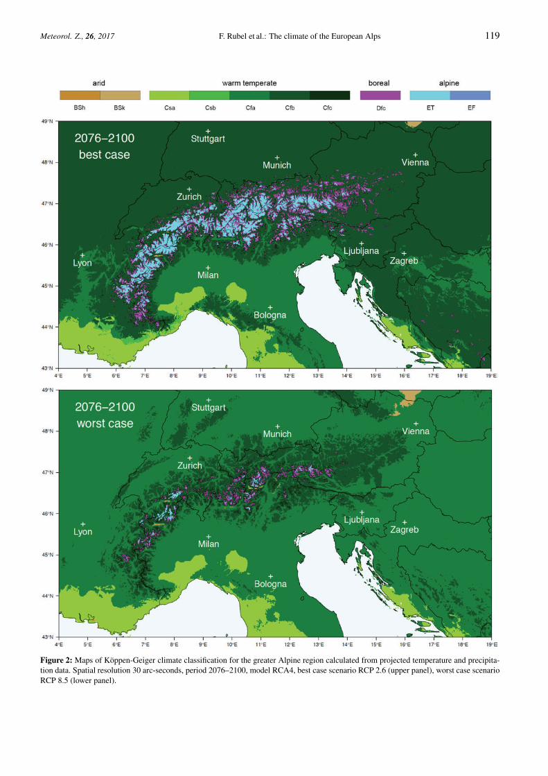
Figure 2: Maps of Köppen-Geiger climate classification for the greater Alpine region calculated from projected temperature and precipita-tion data. Spatial resolution 30 arc-seconds, period 2076–2100, model RCA4, best case scenario RCP 2.6 (upper panel), worst case scenarioRCP 8.5 (lower panel).

120 F. Rubel et al.: The climate of the European Alps Meteorol. Z., 26, 2017

resolution of the maps. Much more important are the fivewarm temperate climates, which cover the main part ofthe greater Alpine region. Within these climates, a dis-tinction is drawn between the occurrence and absenceof a dry season, as well as between cool, warm and hotsummers. The Cfb climate (no dry season, warm sum-mers) is the prevailing climate in the north of the Alpinedivide. The Cfc climate with cool summers is locatedin the montane belt of the Alps, whereas the three re-maining warm temperate climates were observed southof the Alps. The Cfa climate characterizes a temper-ate climate with hot summers and no dry season, whilethe summer dry climates Csa and Csb are sometimesgrouped together and are commonly called Mediter-ranean climate (Shakesby, 2011). The moist boreal cli-mates of the Alps were exclusively classified accord-ing to their temperature regime into Dfb (warm sum-mer) and Dfc (cool summer and cold winter). Note thatKöppen (1936) developed this classification accordingto the tree species predominant in different regions un-der natural conditions. The region of the Cfb climatewas predominantly covered with deciduous forest, ofwhich beech were the main tree species. Oak were thepredominant species of the Dfb climates and spruce ofthe Dfc climate. However, over recent decades, beechesand oaks have been replaced by high performance in-dustrial spruce forest. Due to climate change, the eco-nomic success of these industrial spruce forests is now inquestion. Therefore, today’s Cfb climate should be inter-preted rather as optimal climate for deciduous forest, theDfb climate as mixed forest climate and the Dfc climateas coniferous forest climate. The timber line separatesthe cool boreal climate (Dfc) from the alpine tundra cli-mate (ET), where tree growth is no longer possible. The10 °C isotherm of the warmest month was defined as acriterion. Note that on the scale considered here it is notpossible to distinguish between the forest and the treeline. Altitudes above the alpine tundra were covered bythe alpine frost (EF) climate. This is located above the0 °C isotherm, which is an approximation of the snowline.

Thus it becomes immediately evident that the tem-perature is the essential parameter to classify the Alpineclimate according to Köppen (1936). Precipitation playsa minor role. In the present climate, precipitation isused exclusively to define the BSh and BSk climatesof dry mountain valleys and to determine the bound-ary of the Mediterranean climates, i.e. the summer dryclimates Csa and Csb. The latter cover coastal regionsfrom sea level up to a height of some 100 meters. Thedisaggregation of the precipitation fields by applying aprecipitation-altitude relationships shows therefore onlya minor effect which, however, reflects the general ex-perience. Alternatively, it might be replaced by a simple2-dimensional spline interpolation.

3 ResultsThe main results of this study are 366 observed andpredicted (two scenarios) very high resolution Köppen-

Geiger climate maps for the greater Alpine region cov-ering the period 1800–2100. Both the digital maps, aswell as the underlying digital data, are publicly avail-able for further investigations on the website http://koeppen-geiger.vu-wien.ac.at. Fig. 1 depicts two ofthese maps, one for the 25-year observational period1876–1900 and one for the more recent observationalperiod 1976–2000. While the years 1876–1900 belongto the coldest years of the entire observational period,the years 1976–2000 illustrate the effect of the recentwarming trend. Clearly visible is the strong decline ofthe boreal climates, which are optimal for coniferousand mixed forests. In the 19th century, the boreal cli-mates Dfb and Dfc covered large areas north of the Alpsas well as the Balkans, while they have been pushedback to higher altitudes during recent years. This reduc-tion of the boreal climates becomes more evident whenlooking at climate projections for the period 2076–2100(Fig. 2). For both greenhouse gas concentration scenar-ios, the Dfb climate, i.e. the boreal climate with warmsummers, has almost completely disappeared. In con-trast, the warm temperate Cfc climate, which was stillrare in the 19th century, becomes the typical climate inthe montane belt of the Alps. The two greenhouse gasconcentration scenarios used result in widely differentmaps. While the RCP 2.6, hereinafter referred to as,the best case scenario, assumes that the warming trendwill not continue during the second half of the 21st cen-tury, the RCP 8.5, hereinafter referred to as, the worstcase scenario, assumes that the recent trend of increas-ing temperatures will continue until the year 2100. Theprojections of the climate zones of both scenarios arefar removed from what was observed during the last200 years. The alpine climates ET and EF will be, in par-ticular, will be forced into small areas in the projection(best case scenario) or will disappear almost entirely(worst case scenario). Assuming the worst case scenario,areas recently classed as the Cfb climate (warm sum-mers) will be covered by the Cfa climate (hot summers)in 2076–2100.

Another way to demonstrate climate change byKöppen-Geiger maps is to observe the boundaries. Themost prominent boundary is the mountain timber line.It is not simply a line, but a transition zone between theforest line and the tree line. Note that numerous defi-nitions of the two lines have been given in a variety ofstudies. Moreover, on a local scale, there are often sig-nificant differences between the potential and the currentforest and tree lines (Szerencsits, 2012). By means ofthe Köppen-Geiger climate maps, it is possible to esti-mate the potential timber line for the entire region ofthe European Alps. The timber line divides the Dfc cli-mate, naturally covered by coniferous forests, from thealpine tundra climate ET and is exclusively defined bytemperature, more precisely by the 10 °C isotherm of thewarmest month. As discussed already by Köppen (1919,1920) and confimed by recent research (Jobbágy andJackson, 2000), the 10 °C July isotherm is an admis-sible approximation for the potential timber line in ex-

Meteorol. Z., 26, 2017 F. Rubel et al.: The climate of the European Alps 121

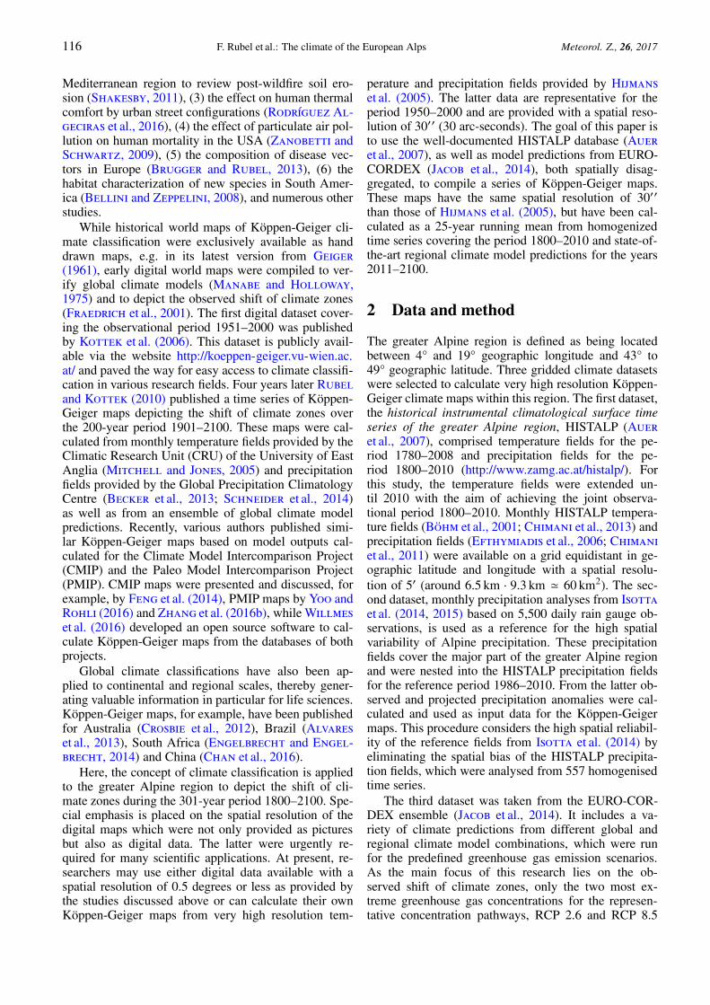
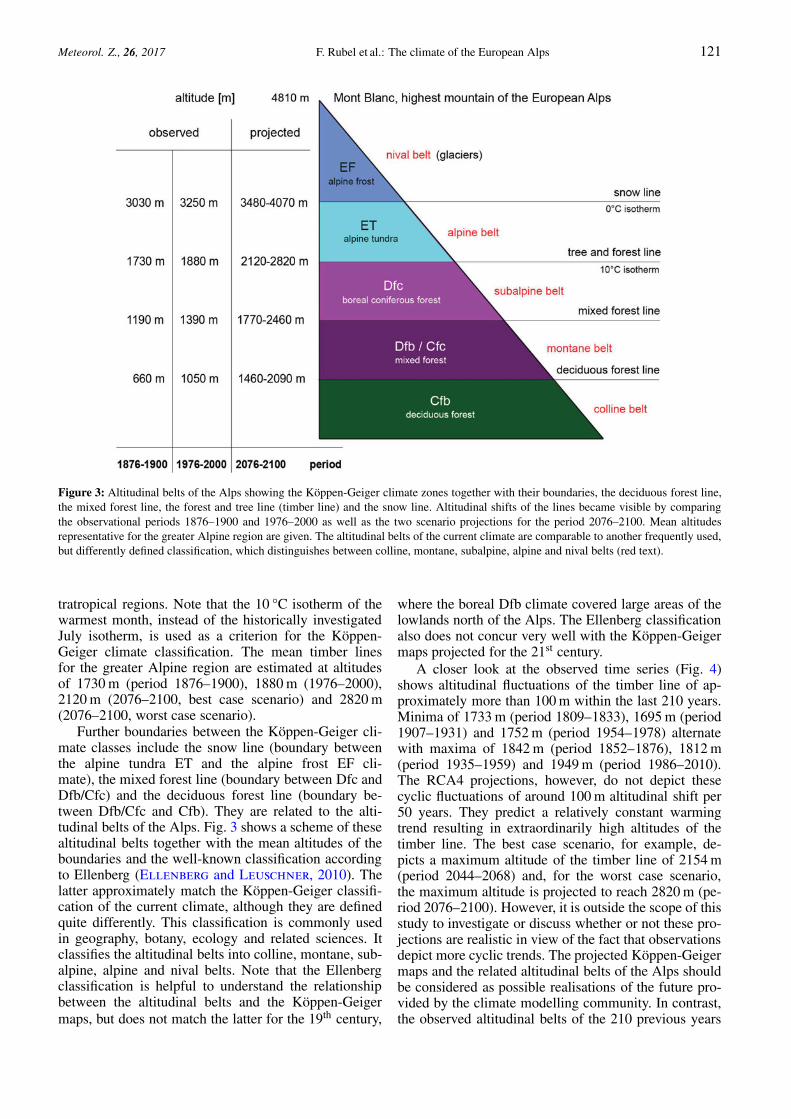
Figure 3: Altitudinal belts of the Alps showing the Köppen-Geiger climate zones together with their boundaries, the deciduous forest line,the mixed forest line, the forest and tree line (timber line) and the snow line. Altitudinal shifts of the lines became visible by comparingthe observational periods 1876–1900 and 1976–2000 as well as the two scenario projections for the period 2076–2100. Mean altitudesrepresentative for the greater Alpine region are given. The altitudinal belts of the current climate are comparable to another frequently used,but differently defined classification, which distinguishes between colline, montane, subalpine, alpine and nival belts (red text).

tratropical regions. Note that the 10 °C isotherm of thewarmest month, instead of the historically investigatedJuly isotherm, is used as a criterion for the Köppen-Geiger climate classification. The mean timber linesfor the greater Alpine region are estimated at altitudesof 1730 m (period 1876–1900), 1880 m (1976–2000),2120 m (2076–2100, best case scenario) and 2820 m(2076–2100, worst case scenario).

Further boundaries between the Köppen-Geiger cli-mate classes include the snow line (boundary betweenthe alpine tundra ET and the alpine frost EF cli-mate), the mixed forest line (boundary between Dfc andDfb/Cfc) and the deciduous forest line (boundary be-tween Dfb/Cfc and Cfb). They are related to the alti-tudinal belts of the Alps. Fig. 3 shows a scheme of thesealtitudinal belts together with the mean altitudes of theboundaries and the well-known classification accordingto Ellenberg (Ellenberg and Leuschner, 2010). Thelatter approximately match the Köppen-Geiger classifi-cation of the current climate, although they are definedquite differently. This classification is commonly usedin geography, botany, ecology and related sciences. Itclassifies the altitudinal belts into colline, montane, sub-alpine, alpine and nival belts. Note that the Ellenbergclassification is helpful to understand the relationshipbetween the altitudinal belts and the Köppen-Geigermaps, but does not match the latter for the 19th century,

where the boreal Dfb climate covered large areas of thelowlands north of the Alps. The Ellenberg classificationalso does not concur very well with the Köppen-Geigermaps projected for the 21st century.

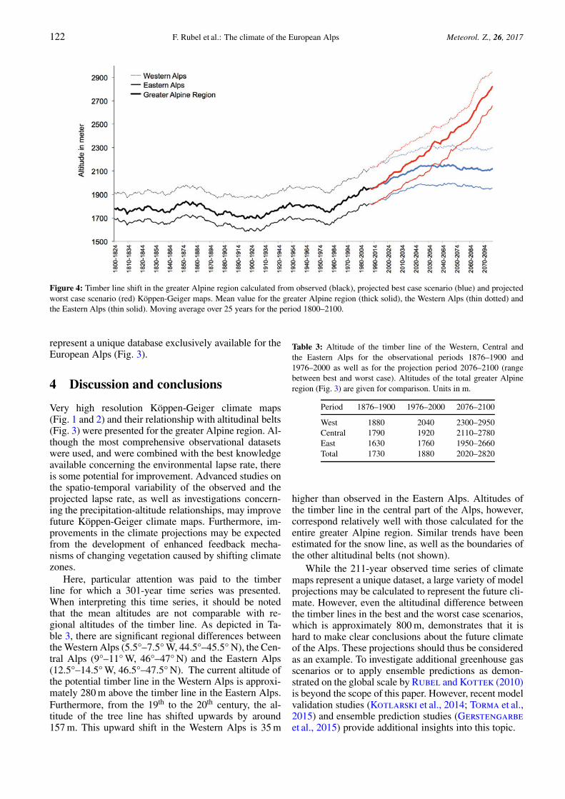
A closer look at the observed time series (Fig. 4)shows altitudinal fluctuations of the timber line of ap-proximately more than 100 m within the last 210 years.Minima of 1733 m (period 1809–1833), 1695 m (period1907–1931) and 1752 m (period 1954–1978) alternatewith maxima of 1842 m (period 1852–1876), 1812 m(period 1935–1959) and 1949 m (period 1986–2010).The RCA4 projections, however, do not depict thesecyclic fluctuations of around 100 m altitudinal shift per50 years. They predict a relatively constant warmingtrend resulting in extraordinarily high altitudes of thetimber line. The best case scenario, for example, de-picts a maximum altitude of the timber line of 2154 m(period 2044–2068) and, for the worst case scenario,the maximum altitude is projected to reach 2820 m (pe-riod 2076–2100). However, it is outside the scope of thisstudy to investigate or discuss whether or not these pro-jections are realistic in view of the fact that observationsdepict more cyclic trends. The projected Köppen-Geigermaps and the related altitudinal belts of the Alps shouldbe considered as possible realisations of the future pro-vided by the climate modelling community. In contrast,the observed altitudinal belts of the 210 previous years

122 F. Rubel et al.: The climate of the European Alps Meteorol. Z., 26, 2017

Figure 4: Timber line shift in the greater Alpine region calculated from observed (black), projected best case scenario (blue) and projectedworst case scenario (red) Köppen-Geiger maps. Mean value for the greater Alpine region (thick solid), the Western Alps (thin dotted) andthe Eastern Alps (thin solid). Moving average over 25 years for the period 1800–2100.

represent a unique database exclusively available for theEuropean Alps (Fig. 3).

4 Discussion and conclusions

Very high resolution Köppen-Geiger climate maps(Fig. 1 and 2) and their relationship with altitudinal belts(Fig. 3) were presented for the greater Alpine region. Al-though the most comprehensive observational datasetswere used, and were combined with the best knowledgeavailable concerning the environmental lapse rate, thereis some potential for improvement. Advanced studies onthe spatio-temporal variability of the observed and theprojected lapse rate, as well as investigations concern-ing the precipitation-altitude relationships, may improvefuture Köppen-Geiger climate maps. Furthermore, im-provements in the climate projections may be expectedfrom the development of enhanced feedback mecha-nisms of changing vegetation caused by shifting climatezones.

Here, particular attention was paid to the timberline for which a 301-year time series was presented.When interpreting this time series, it should be notedthat the mean altitudes are not comparable with re-gional altitudes of the timber line. As depicted in Ta-ble 3, there are significant regional differences betweenthe Western Alps (5.5°–7.5° W, 44.5°–45.5° N), the Cen-tral Alps (9°–11° W, 46°–47° N) and the Eastern Alps(12.5°–14.5° W, 46.5°–47.5° N). The current altitude ofthe potential timber line in the Western Alps is approxi-mately 280 m above the timber line in the Eastern Alps.Furthermore, from the 19th to the 20th century, the al-titude of the tree line has shifted upwards by around157 m. This upward shift in the Western Alps is 35 m

Table 3: Altitude of the timber line of the Western, Central andthe Eastern Alps for the observational periods 1876–1900 and1976–2000 as well as for the projection period 2076–2100 (rangebetween best and worst case). Altitudes of the total greater Alpineregion (Fig. 3) are given for comparison. Units in m.

Period 1876–1900 1976–2000 2076–2100

West 1880 2040 2300–2950Central 1790 1920 2110–2780East 1630 1760 1950–2660Total 1730 1880 2020–2820

higher than observed in the Eastern Alps. Altitudes ofthe timber line in the central part of the Alps, however,correspond relatively well with those calculated for theentire greater Alpine region. Similar trends have beenestimated for the snow line, as well as the boundaries ofthe other altitudinal belts (not shown).

While the 211-year observed time series of climatemaps represent a unique dataset, a large variety of modelprojections may be calculated to represent the future cli-mate. However, even the altitudinal difference betweenthe timber lines in the best and the worst case scenarios,which is approximately 800 m, demonstrates that it ishard to make clear conclusions about the future climateof the Alps. These projections should thus be consideredas an example. To investigate additional greenhouse gasscenarios or to apply ensemble predictions as demon-strated on the global scale by Rubel and Kottek (2010)is beyond the scope of this paper. However, recent modelvalidation studies (Kotlarski et al., 2014; Torma et al.,2015) and ensemble prediction studies (Gerstengarbeet al., 2015) provide additional insights into this topic.

Meteorol. Z., 26, 2017 F. Rubel et al.: The climate of the European Alps 123

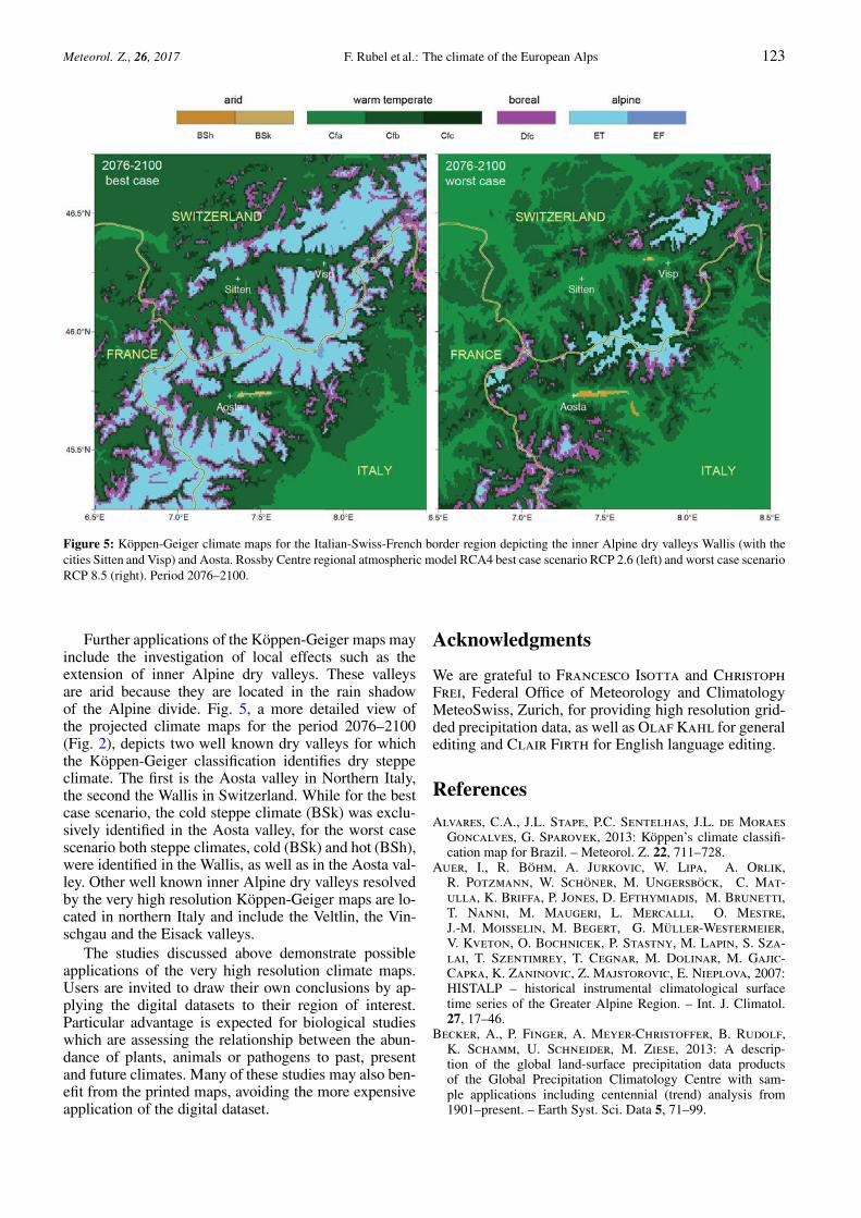
Figure 5: Köppen-Geiger climate maps for the Italian-Swiss-French border region depicting the inner Alpine dry valleys Wallis (with thecities Sitten and Visp) and Aosta. Rossby Centre regional atmospheric model RCA4 best case scenario RCP 2.6 (left) and worst case scenarioRCP 8.5 (right). Period 2076–2100.

Further applications of the Köppen-Geiger maps mayinclude the investigation of local effects such as theextension of inner Alpine dry valleys. These valleysare arid because they are located in the rain shadowof the Alpine divide. Fig. 5, a more detailed view ofthe projected climate maps for the period 2076–2100(Fig. 2), depicts two well known dry valleys for whichthe Köppen-Geiger classification identifies dry steppeclimate. The first is the Aosta valley in Northern Italy,the second the Wallis in Switzerland. While for the bestcase scenario, the cold steppe climate (BSk) was exclu-sively identified in the Aosta valley, for the worst casescenario both steppe climates, cold (BSk) and hot (BSh),were identified in the Wallis, as well as in the Aosta val-ley. Other well known inner Alpine dry valleys resolvedby the very high resolution Köppen-Geiger maps are lo-cated in northern Italy and include the Veltlin, the Vin-schgau and the Eisack valleys.

The studies discussed above demonstrate possibleapplications of the very high resolution climate maps.Users are invited to draw their own conclusions by ap-plying the digital datasets to their region of interest.Particular advantage is expected for biological studieswhich are assessing the relationship between the abun-dance of plants, animals or pathogens to past, presentand future climates. Many of these studies may also ben-efit from the printed maps, avoiding the more expensiveapplication of the digital dataset.

Acknowledgments

We are grateful to Francesco Isotta and ChristophFrei, Federal Office of Meteorology and ClimatologyMeteoSwiss, Zurich, for providing high resolution grid-ded precipitation data, as well as Olaf Kahl for generalediting and Clair Firth for English language editing.

References

Alvares, C.A., J.L. Stape, P.C. Sentelhas, J.L. de MoraesGoncalves, G. Sparovek, 2013: Köppen’s climate classifi-cation map for Brazil. – Meteorol. Z. 22, 711–728.

Auer, I., R. Böhm, A. Jurkovic, W. Lipa, A. Orlik,R. Potzmann, W. Schöner, M. Ungersböck, C. Mat-ulla, K. Briffa, P. Jones, D. Efthymiadis, M. Brunetti,T. Nanni, M. Maugeri, L. Mercalli, O. Mestre,J.-M. Moisselin, M. Begert, G. Müller-Westermeier,V. Kveton, O. Bochnicek, P. Stastny, M. Lapin, S. Sza-lai, T. Szentimrey, T. Cegnar, M. Dolinar, M. Gajic-Capka, K. Zaninovic, Z. Majstorovic, E. Nieplova, 2007:HISTALP – historical instrumental climatological surfacetime series of the Greater Alpine Region. – Int. J. Climatol.27, 17–46.

Becker, A., P. Finger, A. Meyer-Christoffer, B. Rudolf,K. Schamm, U. Schneider, M. Ziese, 2013: A descrip-tion of the global land-surface precipitation data productsof the Global Precipitation Climatology Centre with sam-ple applications including centennial (trend) analysis from1901–present. – Earth Syst. Sci. Data 5, 71–99.

124 F. Rubel et al.: The climate of the European Alps Meteorol. Z., 26, 2017

Bellini, B.C., D. Zeppelini, 2008: Three new species ofSeira Lubbock (Collembola, Entomobryidae) from Mataraca,Para’ba State, Brazil. – Zootaxa 1773, 44–54.

Böhm, R., I. Auer, M. Brunetti, M. Maugeri, T. Nanni,W. Schöner, 2001: Regional temperature variability in theEuropean Alps: 1760–1998 from homogenized instrumentaltime series. – Int. J. Climatol. 21, 1779–1801.

Brugger, K., F. Rubel, 2013: Characterizing the species com-position of European Culicoides vectors by means of theKöppen-Geiger climate classification. – Parasit. Vectors 6,333.

Chan, D., Q. Wu, G. Jiang, X. Dai, 2016: Projected shifts inKöppen climate zones over China and their temporal evolutionin CMIP5 multi-model simulations. – Adv. Atmos. Sci. 33,283–293.

Chimani, B., C. Matulla, R. Böhm, M. Ganekind, 2011: De-velopment of a longterm dataset of solid/liquid precipitation. –Adv. Sci. Res. 6, 39–43.

Chimani, B., C. Matulla, R. Böhm, M. Hofstätter, 2013: Anew high resolution absolute temperature grid for the GreaterAlpine Region back to 1780. – Int. J. Climatol. 33, 2129–2141.

Crosbie, R.S., D.W. Pollock, F.S. Mpelasoka, O.V. Barron,S.P. Charles, M.J. Donn, 2012: Changes in Köppen-Geigerclimate types under a future climate for Australia: Hydrologi-cal implications. – Hydrol. Earth Syst. Sci. 16, 3341–3349.

Diaz-Varela, R.A., R. Colombo, M. Meroni, M.S. Calvo-Iglesias, A. Buffonid, A. Tagliaferri, 2007: Spatio-temporal analysis of alpine ecotones: A spatial explicit modeltargeting altitudinal vegetation shifts. – Ecol. Mod. 221,621–633.

Efthymiadis, D., P.D. Jones, K.R. Briffa, I. Auer, R. Böhm,W. Schöner, C. Frei, J. Schmidli, 2006: Construction of a10-min-gridded precipitation data set for the Greater AlpineRegion for 1800–2003. – J. Geophys. Res. 111, D01105.

Ellenberg, H., C. Leuschner, 2010: Vegetation Mitteleuropasmit den Alpen (Vegetation of Central Europe with the Alps,6th edition). – Eugen Ulmer, Stuttgart, 1334pp.

Engelbrecht, C.J., F.A. Engelbrecht, 2014: Shifts inKöppen-Geiger climate zones over southern Africa in relationto key global temperature goals. – Theor. Appl. Climatol. 123,247–261.

Feng, S., Q. Hu, W. Huang, C.-H. Ho, R. Li, Z. Tang, 2014:Projected climate regime shift under future global warm-ing from multi-model, multi-scenario CMIP5 simulations. –Global Planetary Change 112, 41–52.

Fraedrich, K., F.-W. Gerstengarbe, P.C. Werner, 2001: Cli-mate shift during the last century. – Climate Change 50,405–417.

Frei, C., C. Schär, 1998: A precipitation climatology of theAlps from high-resolution rain-gauge observations. – J. Cli-matol. 18, 873–900.

Geiger, R., 1961: Überarbeitete Neuausgabe von Geiger, R.:Köppen-Geiger / Klima der Erde. (Wandkarte 1:16 Mill.) –Klett-Perthes, Gotha.

Gerstengarbe, F.-W., P. Hoffmann, H. Österle,P.C. Werner, 2015: Ensemble simulations for the RCP8.5-Scenario. – Meteorol. Z. 24, 147–156.

Gottfried, M., M. Hantel, C. Maurer, R. Toechterle,H. Pauli, G. Grabherr, 2011: Climate effects on mountainplants. – Env. Res. Lett. 6, 014013.

Grabherr, G., M. Gottfried, H. Pauli, 1994: Climate effectson mountain plants. – Nature 369, 448–448.

Hantel, M., L.-M. Hirtl-Wielke, 2007: Sensitivity of Alpinesnow cover to European temperature. – Int. J. Climatol. 27,1265–1275.

Hantel, M., C. Maurer, 2011: The median winter snowline inthe Alps. – Meteorol. Z. 20, 267–276.

Haslinger, K., W. Schöner, I. Anders, 2016: Future droughtprobabilities in the Greater Alpine Region based on COSMO-CLM experiments – spatial patterns and driving forces. –Meteorol. Z. 25, 137–148.

Hijmans, R.J., S.E. Cameron, J.L. Parra, P.G. Jones,A. Jarvis, 2005: Very high resolution interpolated climate sur-faces for global land areas. – Int. J. Climatol. 25, 1965–1978.

Isotta, F.A., C. Frei, V. Weilguni, M.P. Tadic, P. Lassègues,B. Rudolf, V. Pavan, C. Cacciamani, G. Antolini,S.M. Ratto, M. Munari, S. Micheletti, V. Bonati, C. Lus-sana, C. Ronchi, E. Panettieri, G. Marigo, G. Vertacnik,2014: The climate of daily precipitation in the Alps: develop-ment and analysis of a high-resolution grid dataset from pan-Alpine rain-gauge data. – Int. J. Climatol. 34, 1657–1675.

Isotta, F.A., R. Vogel, C. Frei, 2015: Evaluation of Europeanregional reanalyses and downscalings for precipitation in theAlpine region. – Meteorol. Z. 24, 15–37.

Jacob, D., J. Petersen, B. Eggert, A. Alias, O.B. Chris-tensen, L. Bouwer, A. Braun, A. Colette, M. Déqué,G. Georgievski, E. Georgopoulou, A. Gobiet, L. Menut,G. Nikulin, A. Haensler, N. Hempelmann, C. Jones,K. Keule, S. Kovats, N. Kröner, S. Kotlarski, A. Kriegs-mann, E. Martin, E. Meijgaard, C. Moseley, S. Pfeifer,S. Preuschmann, C. Radermacher, K. Radtke, D. Rechid,M. Rounsevell, P. Samuelsson, S. Somot, J.-F. Sous-sana, C. Teichmann, R. Valentini, R.Vautard, B. Weber,P. Yiou, 2014: EURO-CORDEX: new high-resolution climatechange projections for European impact research. – Reg. Env.Change 14, 563–578.

Jobbágy, E.G., R.B. Jackson, 2000: Global controls of forestline elevation in the northern and southern hemispheres. –Global Ecol. Biogeogr. 9, 253–268.

Köppen, W., 1919: Baumgrenze und Lufttemperatur (Timberlineand air temperature). – Petermanns Geogr. Mitt. 65, 201–203.

Köppen, W., 1920: Verhältnis der Baumgrenze zur Lufttemper-atur (Relationship between timberline and air temperature). –Meteorol. Z. 37, 39–42.

Köppen, W., 1936: Das geographische System der Klimate (Thegeographic system of climates). – In: Köppen, W., R. Geiger(Hrsg.): Handbuch der Klimatologie, Bd. 1, Teil C. – Born-traeger, Berlin, 44 pp.

Kotlarski, S., K. Keuler, O.B. Christensen, A. Colette,M. Déqué, A. Gobiet, K. Goergen, D. Jacob, D. Lüthi,van E. Meijgaard, G. Nikulin, C. Schär, C. Teichmann,R. Vautard, K. Warrach-Sagi, V. Wulfmeyer, 2014: Re-gional climate modeling on European scales: A joint standardevaluation of the EURO-CORDEX RCM ensemble. – Geosci.Model Dev. 7, 1297–1333.

Kottek, M., J. Grieser, C. Beck, B. Rudolf, F. Rubel, 2006:World map of the Köppen-Geiger climate classification up-dated. – Meteorol. Z. 15, 259–263.

Manabe, S., J.L. Holloway, 1975: The seasonal variation ofthe hydrologic cycle as simulated by a global model of theatmosphere. – J. Geophys. Res. 80, 1617–1649.

Meinshausen, M., S.J. Smith, K. Calvin, J.S. Daniel,M.L.T. Kainuma, J.-F. Lamarque, K. Matsumoto,S.A. Montzka, S.C.B. Raper, K. Riahi, A. Thomson,G.J.M. Velders„ D.P.P. van Vuuren, 2011: The RCPgreenhouse gas concentrations and their extensions from 1765to 2300. – Climatic Change 109, 213–241.

Mitchell, T.D., P.D. Jones, 2005: An improved method of con-structing a database of monthly climate observations and as-sociated high-resolution grids. – Int. J. Climatol. 25, 693–712.

Mizoguchi, Y., A. Miyata, Y. Ohtani, R. Hirata, S. Yuta,2009: A review of tower flux observation sites in Asia. – J. For.Res. 14, 1–9.

Meteorol. Z., 26, 2017 F. Rubel et al.: The climate of the European Alps 125

Rodríguez Algeciras, J.A., L.G. Consuegra,A. Matzarakis, 2016: Spatial-temporal study on theeffects of urban street configurations on human thermalcomfort in the world heritage city of Camagüey-Cuba. –Building Env. 101, 85–101.

Rolland, C., 2003: Spatial and seasonal variations of air tem-perature lapse rates in Alpine regions. – J. Climate 16,1032–1046.

Rubel, F., M. Kottek, 2010: Observed and projected climateshifts 1901–2100 depicted by world maps of the Köppen-Geiger climate classification. – Meteorol. Z. 19, 135–141.

Rubel, F., M. Kottek, 2011: Comments on: ’The thermal zonesof the Earth’ by Wladimir Köppen (1884). – Meteorol. Z. 20,361–365.

Samuelsson, P., C.G. Jones, U. Willén, A. Ullerstig,S. Gollvik, U. Hansson, C. Jansson, E. Kjellström,G. Nikulin, K. Wyser, 2011: The Rossby Centre RegionalClimate model RCA3: model description and performance. –Tellus 63A, 4–23.

Santini, M., di A. Paola, 2015: Changes in the world rivers’discharge projected from an updated high resolution dataset ofcurrent and future climate zones. – J. Hydrol. 531, 768–780.

Schneider, U., A. Becker, P. Finger, A. Meyer-Christoffer,M. Ziese, B. Rudolf, 2014: GPCC’s new land surface precip-itation climatology based on quality-controlled in situ data andits role in quantifying the global water cycle. – Theor. Appl.Climatol. 115, 15–40.

Schwarb, M., C. Frei, C. Schär, C. Daly, 2000: Mean annualprecipitation throughout the European Alps 1971–1990. In:Hydrological Atlas of Switzerland, Plates 2.6. – Federal Officefor Water and Geology, Bern.

Shakesby, R.A., 2011: Post-wildfire soil erosion in the Mediter-ranean: Review and future research directions. – Earth-Sci.Rev. 105, 71–100.

Strandberg, G., L. Bärring, U. Hansson, C. Jansson,C. Jones, E. Kjellström, M. Kolax, M. Kupiainen,G. Nikulin, P. Samuelsson, A. Ullerstig, S. Wang, 2014:CORDEX scenarios for Europe from the Rossby Centre re-gional climate model RCA4. – Report Meteor. Climatol. No.116, SMHI, Norrköping, Sweden.

Szerencsits, E., 2012: Swiss tree lines – a GIS-based approxi-mation. – Landscape Online 28, 1–18.

Theurillat, J.-P., A. Guisan, 2001: Potential impact of climatechange on vegetation in the European Alps: A review. – Cli-matic Change 50, 77–109.

Torma, C., F. Giorgi, E. Coppola, 2015: Added value of re-gional climate modeling over areas characterized by complexterrain – Precipitation over the Alps. – J. Geophys. Res. At-mos. 120, 3957–3972.

Willmes, C., D. Becker, S. Brocks, C. Hütt, G. Bareth,2016: High resolution Köppen-Geiger classifications of paleo-climate simulations. – Trans. in GIS, DOI:10.1111/tgis.12187.

Yoo, J., R.V. Rohli, 2016: Global distribution of Köppen-Geiger climate types during the Last Glacial Maximum,Mid-Holocene, and present. – Palaeogeogr. Palaeoclimatol.Palaeoecol. 446, 326–337.

Zanobetti, A., J. Schwartz, 2009: The effect of fine andcoarse particulate air pollution on mortality: A national analy-sis. – Env. Health Perspect. 117, 898–903.

Zhang, C., D. Lu, X. Chen, Y. Zhang, B. Maisupova, Y. Tao,2016a: The spatiotemporal patterns of vegetation coverageand biomass of the temperate deserts in Central Asia and theirrelationships with climate controls. – Remote Sens. Environ.175, 271–281.

Zhang, L., C. Wang, X. Li, K. Cao, Y. Song, B. Hu, D. Lu,Q. Wang, X. Du, S. Cao, 2016b: A new paleoclimateclassification for deep time. – Palaeogeogr. Palaeoclimatol.Palaeoecol. 443, 98–106.