Embed Size (px)
Citation preview
1
The Choice of Mean Reversion Stochastic Process for
Real Option Valuation
Carlos de Lamare Bastian-Pinto Management Department – Ibmec Business School
Av. Presidente Wilson 118 - Centro - Rio de Janeiro, 20030-020, RJ, Brasil +55 21 9496-5520
Luiz Eduardo Teixeira Brandão IAG Business School - Pontifícia Universidade Católica - Rio de Janeiro Rua Marques de São Vicente 225 - Rio de Janeiro, 22451-900, RJ, Brasil
+ 55 21 2138-9304 [email protected]
Luiz de Magalhães Ozorio Management Department – Ibmec Business School
Av. Presidente Wilson 118 - Centro - Rio de Janeiro, 20030-020, RJ, Brasil +55 21 9923-1747

2
The Choice of Mean Reversion Stochastic Process for
Real Option Valuation
Abstract:
A main issue in financial derivatives and real options valuation is the choice of an adequate stochastic
model to describe the price dynamics of the underlying asset. Particularly, in investment projects
where there is significant managerial flexibility, the choice of stochastic process can have significant
impacts on the project value and, therefore, the investment rule. This paper discusses several criteria
for stochastic processes selection between Brownian Motion and Mean Reversion and the related
theoretical, as well as practical, issues concerning the application of these to real options valuation.
Empirical examples are used to illustrate the methods described along with guidelines for their
implementation.
Key-words:
Mean Reversion Model, Geometric Brownian Motion, Stochastic Processes, Real Options
JEL codes:
C15, C53, G13, M21.
3
1 Introduction
Investment decisions involving stocks, financial derivatives and corporate projects are
influenced by several sources of uncertainties. One way of dealing with these a priori
unexplained market movements is the statistical modeling of the asset prices that relate to the
specific problem at hand. The choice of an adequate statistical time series model (or, should
one prefer, stochastic process; or stochastic model) plays a central role, for instance, in real
option valuation, impacting not only the project value itself, but also the investment rule
(Dixit & Pindyck, 1994; Schwartz, 1997).
In financial derivatives valuation, the geometric Brownian motion (GBM) is frequently
assumed to be an appropriate choice to describe the behavior of stock prices and indexes
(Black & Scholes, 1973; Cox et al., 1979). GBM has also been largely used in corporate
project valuation using real options analysis (Trigeorgis, 1993). On the other hand, with
commodities related projects and derivatives valuation, mean reversion models (MRM) have
become a recurrent choice (Schwartz 1997, Gibson & Schwartz, 1990; Pindyck, 1999;
Schwartz & Smith, 2000). The rationale behind this derives from micro-economics: while
commodity price wanders randomly in the short term, they tend to converge to an equilibrium
level in the long term, mirroring their marginal cost of production. Nevertheless, it is rarely
easy to determine which model – GBM, or MRM – is a more adequate choice for modeling
uncertain variables. Some of the questions that must be taken into account in the choice of an
adequate stochastic process for modeling a particular derivative on an underlying asset are: (i)
the economic features of the corresponding underlying asset; (2) the derivative lifetime; (3)
the numerical and statistical issues regarding parameter estimation; and (4) the applicability of
the chosen process in solutions (analytical or numerical) of the models used to valuation,
among other factors.
This paper discusses several criteria for selecting an appropriate single factor stochastic
process in real option valuation. Some of the generally adopted stochastic processes are
briefly presented (GBM and MRM) and some statistical methods for model selection are
revisited (unit root tests and variance ratio tests). Furthermore we propose the use of
parameter ratios to better determine the adequacy of each process. Empirical examples
involving nine commodities time series (three energy, three metals and three agricultural) are

4
also provided for assessing the performance of the methods with real data sets. As an
important complement, some guidelines regarding economic theory considerations, assets
lifetime, numerical issues in parameter estimation, and the difficulties in real option valuation
are suggested.
This paper is structured as follows: after this introduction, Section 2 offers, without claiming
exhaustiveness, a review of the literature on some single factor stochastic processes frequently
considered in real option analyses and their basic mathematical properties. Section 3 describes
in some detail the statistical framework under which stochastic model selection is
implemented; in this section, some empirical examples are given to illustrate the techniques.
Section 4 suggests guidelines to future users of the methods discussed and in Section 5 we
conclude by listing the main findings and a suggestion of themes for future research.
2 Single Factor Stochastic Processes in Real Option Valuation
We can define stochastic process as variables that move discretely or continuously in time
unpredictably or, at least, partially randomly. Formally, let Ω be a set that represents the randomness,
where Ω∈w denotes a state of the world and f a function which represents a stochastic process. The
function f depends on Rx∈ e Ω∈w : RR →Ω× or ),( wxf , and it has the following property:
given Ω∈w , ),( wf o becomes a function of only x. Thus, for different values of Ω∈w we get
different functions of x. When x represents time, we can interpret ),( 1wxf and ),( 2wxf as two
different trajectories that depend on different states of the world, as we can see in Figure 1:
Figure 1 – Stochastic process trajectories.
x(t,w
)
t
x(t,w1)
x(t,w2)

5
In investment decisions, such as with real option valuation, the appropriate choice of the stochastic
process used for modeling the dynamics of the asset prices involved is a matter of great relevance,
since the forecasting and/or simulation of future cash flows crucially depends on conditional
probability distributions of future trajectories. In the case of real options valuation, in which the
uncertainties are directly considered in the future cash flow of the assets, the relevance is even greater.
A class of stochastic processes that plays an important role in financial modeling are Markov
Processes. In a Markov Process, only the latest observed value is considered to be relevant to forecast
future values. Such condition is commonly referred as the Markov property and is consistent with the
Weak Form of Market Efficiency. One of the most popular types of Markov Processes is the
Geometric Brownian Motion, which has been traditionally used in the modeling of financial options
(Black & Scholes, 1973) and real option (Brennan & Schwartz, 1985; McDonald & Siegel, 1985,
1986; Paddock, Siegel, & Smith, 1988).
GBM is a continuous time process and is defined by equation (1).
xdzxdtdx σα += , (1)
where:
x is the asset price; α is the drift parameter; σ is the volatility parameter; dt is the time increment; dz is the standard Wiener increment.
Some interesting features of GBM, which are part of the reason for its popularity, are the small
number of parameters that need to be estimated and the ease of application of analytical and numerical
solutions for asset valuation. However, it has as a major drawback the fact that, under this model with
a nonzero drift parameter, asset prices trajectories diverge with probability 1 as time increases. And,
even considering a null drift parameter, its variance grows proportionally with time. Therefore,
projected or simulated price trajectories could create unrealistic scenarios, which is an undesirable
property in the case of long term assets. Figure 2 displays several simulated price trajectories from a
GBM with a positive drift (on the left side) and the corresponding frequency distribution of a 20.000
events simulation; one can readily notice both the mean and the variance of the process increasing
with time.

6
Figure 2 – GBM Price simulation 120 trajectories (l eft), with: ∆t = 0.1; α = 0.1 and σ = 0.2;
and corresponding density distributions for 20,000 simulations (right).
But with some variables, for which there are evidences and economic considerations supporting the
claim that uncertainties in prices maintain an equilibrium level, such as in the case of commodities
prices and interest rates, the appropriateness of the GBM has been vastly questioned (Bhattacharya,
1978; Brennan & Schwartz, 1985; Lund, 1993; Metcalf & Hasset, 1995; Smith & McCardle, 1998;
Pindyck, 1999, 2001; Geman, 2005; Al-Harthy, 2007). Focusing on commodities, such as oil, copper,
sugar or ethanol, it is common practice to assume that prices are at least partially driven by mean-
reversion components, which makes these wander randomly in short term, but tend to converge to the
equilibrium level in the long term, reflecting their marginal costs of production. A well-known mean
reversion model (MRM) is the Ornstein Uhlenbeck (OU) model, whose expression, for its continuous-
time version, is displayed in equation (2):
dzdtxxdx ση +−= )( (2)
where:
x is the asset price; x is the equilibrium level to which the process reverts in the long run; η is the speed of reversion parameter;
σ is the volatility parameter; dzis the standard Wiener increment.
Although the MRM is also a Markov process, its increments are not independent, as opposed to the
case of the GBM. Also, as it is an arithmetic model, the use of the Ornstein-Uhlenbeck model for
simulating future price paths might result in negative values. To avoid such inconvenience, it is useful
to consider that the logarithm of prices follow an OU process, such as in Schwartz (1997), and prices
therefore follow a geometric MRM. Figure 3 presents simulated trajectories for such an MRM.
0 1 2 3 4 5 6 7 8 9 100
50
100
150
200
250
300
350
400
450
500
t
$
01
23
45
67
89
10 0
10
20
30
40
50
0
2000
4000
x 10 $t
Eve
nts

7
Figure 3 –MRM Price simulation 120 trajectories (le ft), with: ∆t = 0.1; η = 0.5;σ = 0.2; x0 =100; = 200; and corresponding density distributions for 20,000 simulations (right).
Other authors (Gibson & Schwartz, 1990; Schwartz, 1997; Pindyck, 1999; Schwartz & Smith, 2000)
focused on the stochastic behavior of commodity prices.
These authors claim that, besides a MRM factor, commodities prices may also have a stochastic trend
factor. From the practical standpoint, such trend factor would alter the equilibrium level to which the
process reverts in the long run. These changes would have additional motivations to momentary
mismatches of supply and demand (captured by MRM) and they could be caused by the progressive
exhaustion of natural resources and incremental costs related to new requirements of environmental
laws, among other issues yielding a steady increase in the equilibrium level. On the other hand,
improvements in the exploration and production technologies might yield a downward trend. Schwartz
& Smith (2000) give support to these economic standpoints and propose a two-factor model, with a
GBM and a MRM correlated components. The sum of these two stochastic factor results in the
logarithm of the asset price, as it can be seen in eq.(6):
ln St = χt + ξt (6)
where:
St is the spot price of the commodity; χt is the factor which represents the changes of the prices in short term; ξt is the factor which represents the tendency of the prices in the long run. The differential equations of the two stochastic processes are: dχt = -κ χtdt + σχdzχ dξt = µξdt + σξdzξ
dzχdzξ = ρdt
where:
κ is the speedy of reversion parameter of the MRM component; σχ is the volatility parameter of the short run changes in prices;
0 1 2 3 4 5 6 7 8 9 100
50
100
150
200
250
300
350
400
450
500
01
23
45
67
89
10 0
1020
3040
50
0
2000
4000
x 10 $t
Eve
nts

8
dzχ is the Wiener increment of the short run changes in prices; µξ is the drift parameter of the long run price tendency; σξ is the volatility parameter of the long run price tendency; dzξ is the Wiener increment of the long run price tendency; ρ is the correlation parameter of the two factor increments.
In order to estimate the necessary parameters, the authors use future prices of commodities and applied
the state space modeling approach combined with the Kalman filter (cf. Harvey, 1989; and Durbin &
Koopman, 2001). But these examples of stochastic processes are multiple factor processes, and thus
involve a significant level of complexity in parametrization as well as modeling, and will not be
covered in this paper. Table 1 summarizes the different types of stochastic processes that have been
briefly revisited so far in this paper.
Table 1 - Stochastic processes used in real options valuation.
Type of Stochastic Process References
One Factor Models
GBM Paddock, Siegel & Smith (1988)
MRM Dixit & Pindyck (1994),
Schwartz (1997, model 1)
MRM with drift Ozorio, Bastian-Pinto, Baidya & Brandao (2012)
Multiple Factor Models
Combination of MRM and GBM
Gibson & Schwartz (1990),
Schwartz (1997, models 2 & 3),
Schwartz & Smith (2000)
3 Approaches for selecting stochastic processes
Some statistical tools, as well as time series parameter estimation, can be useful in the investigation of
how much adequate a stochastic models is for asset price dynamics description. In this section we
discuss three of these tools in some detail: (1) a unit root test; (2) the variance ratio test; and (3)
parameter estimation and calibration.
3.1 Dickey-Fuller, or Unit Root test
The Dickey-Fuller (DF) unit root test (cf. Wooldridge, 2000; Enders, 2004) is frequently used to
statistically assess if a commodity price is non-stationary. This test involves estimating a first-order
autoregressive model for the lagged log of prices (Eq. (7)) and testing whether the autoregressive
9
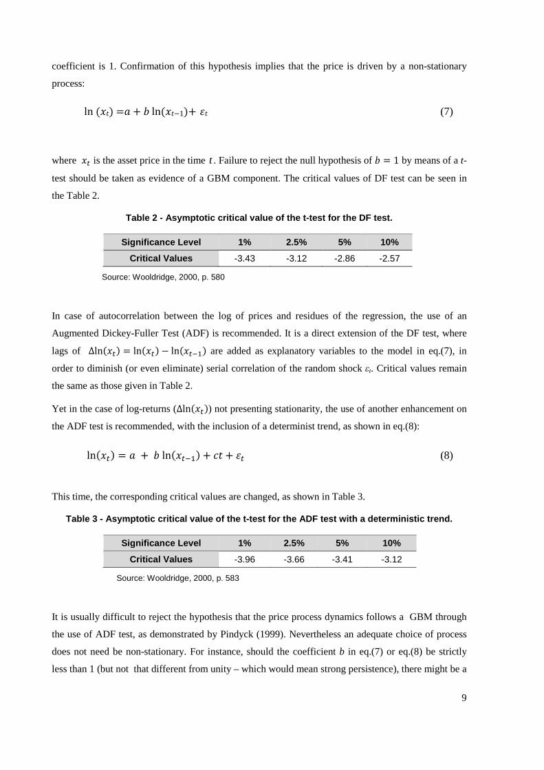
coefficient is 1. Confirmation of this hypothesis implies that the price is driven by a non-stationary
process:
ln () = + ln(−1)+ (7)
where is the asset price in the time t . Failure to reject the null hypothesis of = 1 by means of a t-
test should be taken as evidence of a GBM component. The critical values of DF test can be seen in
the Table 2.
Table 2 - Asymptotic critical value of the t-test f or the DF test.
Significance Level 1% 2.5% 5% 10%
Critical Values -3.43 -3.12 -2.86 -2.57
Source: Wooldridge, 2000, p. 580
In case of autocorrelation between the log of prices and residues of the regression, the use of an
Augmented Dickey-Fuller Test (ADF) is recommended. It is a direct extension of the DF test, where
lags of Δln() = ln() − ln() are added as explanatory variables to the model in eq.(7), in
order to diminish (or even eliminate) serial correlation of the random shock εt. Critical values remain
the same as those given in Table 2.
Yet in the case of log-returns (Δln()) not presenting stationarity, the use of another enhancement on
the ADF test is recommended, with the inclusion of a determinist trend, as shown in eq.(8):
ln() = + ln() + + (8)
This time, the corresponding critical values are changed, as shown in Table 3.
Table 3 - Asymptotic critical value of the t-test f or the ADF test with a deterministic trend.
Significance Level 1% 2.5% 5% 10%
Critical Values -3.96 -3.66 -3.41 -3.12
Source: Wooldridge, 2000, p. 583
It is usually difficult to reject the hypothesis that the price process dynamics follows a GBM through
the use of ADF test, as demonstrated by Pindyck (1999). Nevertheless an adequate choice of process
does not need be non-stationary. For instance, should the coefficient b in eq.(7) or eq.(8) be strictly
less than 1 (but not that different from unity – which would mean strong persistence), there might be a

10
presence of MRM dynamics, even in cases where the GBM has not been formally rejected. In order to
illustrate these difficulties Dixit & Pindyck (1994) applied these unit root tests with 30 and 40-year
price series and were not able to reject the hypothesis that oil prices would follow a GBM. It was
necessary to make tests with 120-year series for the formal rejection of a unit root.
One way to verify the consistency of ADF test results is with the use of a complementary test: the
Kwiatkowski–Phillips–Schmidt–Shin (KPSS) test, which can be used for checking a null hypothesis
that a variable is stationary around a deterministic trend. KPSS type tests are intended to complement
unit root tests, such as the Dickey–Fuller tests. Therefore when testing both the unit root (DF) and the
stationarity (KPSS) hypothesis, one can distinguish series that appear to be stationary, series that
appear to have a unit root, and series for which the data (or the tests) are not sufficiently informative to
be sure whether they are in fact stationary.
Table 4 - Asymptotic critical value of the t-test f or the KPSS test with a deterministic trend.
Significance Level 1% 2.5% 5% 10%
Critical Values 0.216 0.184 0.146 0.199
If it is not possible to consistently reject the presence of a unit root at a significant level, which would
imply adequacy of a GBM modeling, running the KPSS test checks the stationarity of the series:
rejection of it confirms the presence of some degree of mean reversion.
3.2 Variance Ratio Test
A second approach that can be used for investigating how adequate a stochastic model is for the price
generating process, is to verify whether the variance of the log of prices increases proportionally to the
lag considered. This approach measures how much the level of the stochastic shocks are persistent.
With autoregressive processes – such as MRM – shocks tend to dissipate when there is a permanent
reversion strength. In contrast, with GBM – which is not an autoregressive process – the shocks in
prices are persistent, which is a necessary condition for the adequacy of the GBM. For such a task,
Pindyck (1999) proposed a variance ratio test which consists of verifying if the variance of the log of
prices increases proportionally in time. Rigorously speaking, this is not a statistical test in the formal
sense. Instead, this is a simple, albeit quite powerful, graphical observation mean that works as
follows. The “test statistic” measures the level to where the variance converges as the lags in the log
returns increase, as shown in Eq. (9):
( )( )1
ln ln1
ln lnt k t
kt t
Var P PR
k Var P P+
+
−=
−, (9)

11
where ( ).Var denotes the sample variance. Should GBM be an adequate dynamic for P , then we
would expect that variance increases proportionally and linearly with the lag of k periods, implying
that Rk would converge to 1 as k grows indefinitely. Alternatively, in case of a MRM the variance is
bounded to a certain level, implying that Rk will decrease, tending to zero, as k grows.
3.3 Parameter Indicators: Half-Life (T1/2) and Normalized Variance (NVar)
Parameter estimation for different stochastic models can be quite revealing and useful for
determination of the stochastic behavior of a time series. As seen with the variance ratio test, GBM
assumes that stochastic shocks are permanent and do not dissipate with time. Also variance of the
variable return should grow proportionally to time. In the case MRM the opposite happens: not only is
the variance limited to a boundary as time increases but stochastic shocks also tends to dissipate under
the effect of the mean reversing force or speed. Thus, estimation of the mean reverting speed
parameter η and its intensity can clearly indicate how much mean reverting the time series has been
behaving as.
As the Mean Reversion Speed Parameter η is estimated in a time basis but is not very indicative of its
intensity (does a parameter of η = 0.2 indicate a strong mean reversion? And 0.5?) we can convert it to
a less elusive magnitude. We can think of the half-life of a Mean Reverting time series in the same
way we think of the half-life of a radioactive compound. The radioactive half-life for a given
radioisotope is the time required for half the radioactive nuclei in a sample to undergo radioactive
decay. Similarly, the half-life (T1/2) of a time series indicates the expected time required for the S value
of a series to reach half the separation it has now from the equilibrium level , given the mean
reversion deterministic dynamics. Or, equivalently, the time for the stochastic shock to dissipate half
of its effect on the time series values. The half-life (T1/2) is inversely proportional to the mean
reversion speed parameter and can be calculated by equation (10).
/ =()
(10)
As it is a time measure, it provides a more intuitive indication of mean reversion force than the mean
reversion parameter itself.
Another parameter which is also highly indicative of the presence of mean reversion is the value to
which the variance of the series converges as the lime lag increases. In the presence of Brownian

12
Motion, variance tends to increase continuously in time, while under Mean Reversion, variance is
restricted to limit value since the reversion force tends to dissipate the volatility of the series. This
limit value is also inversely proportional to twice the mean reversion speed parameter and directly
proportional to the square of the volatility parameter, and therefore is referred to as the Normalized
Variance (NVar) parameter of the series. The NVar can be estimated by equation (11).
! ="#
(11)
A graphical representation of the measurement of those parameters on the expected value of a time
series is shown in Figure 4.
Figure 4 – Half-Life ( T1/2) Indication and Normalized Variance ( NVar)
of a Mean Reversion Time Series
Although both measures are inversely proportional to η, each indicates one characteristic of mean
reversion: the half-life indicates about half the cycle involved in the dynamics present in a series. If is
it too long (i.e. several years) mean reversion is hardly present in these dynamics. Likewise, if the
normalized variance is too high it is unlikely that such a series are reverting to an equilibrium level,
since its stochastic process (proportional to σ) dominates the dampening effect of the mean reversion
(quantified by η).
4 Testing with Spot Prices Time Series
If order to illustrate application of the measures explained in chapter 3, we test nine different types of
data sets of commodity prices: thirty three years of monthly closing spot prices (from December 1982
to December 2015) for Natural Gas (Henry Hub, data available only from 1991 on), Oil (Brent), Coal
(Australian Thermal), Copper, Nickel, Aluminum, Soybeans, Cotton and Coffee (Other Mild
Arabicas). These series are available through CBE group site and are displayed in Figures 5.
0
T1/2 =

13
It is interesting to note that these series are highly volatile, and with great amplitude of their range as,
in some cases, the high values are up to ten times greater than the low values during the time span
studied. They also cover energy (black lines), metal (blue lines) and agricultural (green) commodities,
covering a wide range of different products. Although they are historical data, the effect of inflation,
will be covered in a specific chapter later on this paper. Also note that all graph in Figure 5 have 0 as
their minimal value in the y axis, therefore they can be directly compared one to another.
A first visual inspection suggests that Aluminum and Coffee clearly display mean reversion behavior,
while Cotton only marginally so. All others show clear trend or level change during the time span.
Figure 5 –Commodity monthly prices - Source: CBE Gr oup
0
2
4
6
8
10
12
19
83
19
85
19
87
19
89
19
91
19
93
19
95
19
97
19
99
20
01
20
03
20
05
20
07
20
09
20
11
20
13
20
15
US
ce
nts
/Me
tric
To
nx
10
00
Copper
0
10
20
30
40
50
60
19
83
19
85
19
87
19
89
19
91
19
93
19
95
19
97
19
99
20
01
20
03
20
05
20
07
20
09
20
11
20
13
20
15
US
$ c
en
ts/
me
tric
to
nx
10
00
Nickel
0
100
200
300
400
500
600
700
19
83
19
85
19
87
19
89
19
91
19
93
19
95
19
97
19
99
20
01
20
03
20
05
20
07
20
09
20
11
20
13
20
15
US
$/m
etr
ic t
on
Soybeans
0
50
100
150
200
250
19
83
19
85
19
87
19
89
19
91
19
93
19
95
19
97
19
99
20
01
20
03
20
05
20
07
20
09
20
11
20
13
20
15
US
ce
nts
/Po
un
d
Cotton
0
1
1
2
2
3
3
4
4
19
83
19
85
19
87
19
89
19
91
19
93
19
95
19
97
19
99
20
01
20
03
20
05
20
07
20
09
20
11
20
13
20
15
US
$ c
en
ts/
me
tric
to
nx
10
00
Aluminum
0
50
100
150
200
250
300
350
19
83
19
85
19
87
19
89
19
91
19
93
19
95
19
97
19
99
20
01
20
03
20
05
20
07
20
09
20
11
20
13
20
15
US
ce
nts
pe
r P
ou
nd
Coffee
0
2
4
6
8
10
12
14
16
19
83
19
85
19
87
19
89
19
91
19
93
19
95
19
97
19
99
20
01
20
03
20
05
20
07
20
09
20
11
20
13
20
15
US
$ m
mB
tu
Natural Gas - Henry Hub
0
20
40
60
80
100
120
140
1601
98
31
98
51
98
71
98
91
99
11
99
31
99
51
99
71
99
92
00
12
00
32
00
52
00
72
00
92
01
12
01
32
01
5
US
$ B
arr
el
Crude Oil - Dated Brent
0
20
40
60
80
100
120
140
160
180
200
19
83
19
85
19
87
19
89
19
91
19
93
19
95
19
97
19
99
20
01
20
03
20
05
20
07
20
09
20
11
20
13
20
15
US$
ce
nts
/ m
etr
ic t
on
Coal, Australian thermal

14
All nine series (log returns) are tested for unit foot presence, using DF, ADF and also KPSS, for trend
and intercept in E-Views software. Results of these are displayed in Table 5.
Table 5 – Unit Root Tests – Series 1982 - 2015.
Test Nat Gas
Oil
Brent
Coal
Austr Copper Nickel Aluminum Soybeans Cotton Coffee
DF -2.956* -2.072 -1.923 -2.400 -2.567 -2.500 -2.565 -3.608+ -2.459
ADF -2.924 -2.859 -2.539 -2.444 -2.666 -2.931 -2.954 -3.635* -2.616
KPSS 0.251+ 0.502
+ 0.413
+ 0.303
+ 0.158* 0.099 0.372
+ 0.195* 0.282
+
Statistical Significance: + : 1% ; *: 5%
These same ADF results are displayed graphically in Figure 6 for a better estimation of significance.
Figure 6 –ADF test results
Contrary to expectation for ADF, only Cotton series reject the presence of a unit root and only at a 5%
level of significance, suggesting that all other series of price should not be modeled as MRM.
Aluminum, Natural Gas, Oil and Soybeans come close to a 10% level and Coffee contrary to
expectations stays clearly out of rejection range.
Use of the variance ratio test is also applied to the same time series. Figure 7 displays the results of the
variance ratio test with these, and as can be observed after initially rising above the unity, for most
series the variance ratio drops below 1 after a lag of about 30 to 60 months. Differently Coal and
Copper stay above unity for all the time span of 120 months (10 years) clearly sustaining that for these
prices, variance keeps growing with time indicating the presence of a GBM. In the case of Natural
Gas, Oil and Soybeans, the ration drops below unity rather rapidly but only with Natural Gas it keeps
going down below 0.5. With Oil and Soybeans prices variance ratio stabilizes above 0.5 for the
-4,5
-4,0
-3,5
-3,0
-2,5
-2,0
-1,5
-1,0
-0,5
0,0
10%
5%
1%

15
duration of the analyzed time span. With Nickel, Aluminum, Cotton and Coffee, the ratio drops below
1 after a higher value of k (lag) but only with Aluminum does it continue dropping clearly below 0.5.
A variance ratio below 1 is a strong indication that the prices are certainly not exclusively driven by
GBM dynamics, and that an MRM type of process might prove to be more suitable for stochastic
modeling of theses series, or at least be also present.
These results indicate that Coal and Copper are clearly GBM type of series, Natural Gas and
Aluminum can be modeled with MRM type of dynamics, and all others display presence of both type
of dynamics in their behavior (GBM and MRM).

16
Figure 8 –Variance Ratio tests of Spot Price Series
As a tie breaker, we then estimate the parameters indicators for all nine time series for modeling these
as GBM and MRM. For this last stochastic model we consider the Schwartz (1997) model 1 type of
single factor geometric MRM. Basic parameters (drift and volatility, α, σ for GBM and reversion
speed, volatility and equilibrium level) where calculated based on the log return of the series, and
equations of Appendix 1. With these we calculated the Half-life time and Normalized Variance for all
nine time series. These are displayed in Table 6, all parameters are in yearly values.
0
0,5
1
1,5
2
0 10 20 30 40 50 60 70 80 90 100 110
Va
r R
ati
o
Lag
Soybeans
0
0,5
1
1,5
2
0 10 20 30 40 50 60 70 80 90 100 110
Va
r R
ati
o
Lag
Cotton
0
0,5
1
1,5
2
0 10 20 30 40 50 60 70 80 90 100 110
Va
r R
ati
o
Lag
Coffee
0
0,5
1
1,5
2
0 10 20 30 40 50 60 70 80 90 100 110
Va
r R
ati
o
Lag
Copper
0
0,5
1
1,5
2
0 10 20 30 40 50 60 70 80 90 100 110
Va
r R
ati
o
Lag
Nickel
0
0,5
1
1,5
2
0 10 20 30 40 50 60 70 80 90 100 110
Va
r R
ati
oLag
Aluminum
0
0,5
1
1,5
2
0 10 20 30 40 50 60 70 80 90 100 110
Va
r R
ati
o
Lag
Natural Gas
0
0,5
1
1,5
2
0 10 20 30 40 50 60 70 80 90 100 110
Va
r R
ati
oLag
Oil - Brent
0
0,5
1
1,5
2
0 10 20 30 40 50 60 70 80 90 100 110
Va
r R
ati
o
Lag
Coal Austr

17
Table 6 – Parameters – Series 1982 - 2015
Natural
Gas Oil
Brent Coal
Austr. Copper Nickel Alumin. Soybean Cotton Coffee
MGB
Drift α 3.1% 1.2% 1.0% 3.8% 3.3% 1.4% 1.6% 0.1% 0.5%
Vol σ 40.1% 30.9% 18.8% 22.0% 29.7% 19.8% 19.9% 19.7% 27.4%
MRM
Rev Speed η 0.41 0.09 0.07 0.07 0.16 0.34 0.17 0.27 0.23
Vol σ 46.2% 31.1% 18.9% 22.1% 29.8% 20.0% 20.0% 19.9% 27.6%
Parameter Indicator
Half-life: T1/2 1.7 7.5 10.3 10.2 4.2 2.1 4.1 2.6 3.0
NVar : σ2/2η 0.26 0.52 0.27 0.36 0.27 0.06 0.12 0.07 0.17
In order to better compare these results, we plotted them in Figure 9 with Half-life as x and
Normalized Volatility as y axis. The closer the series are situated to the axis origins, the more MRM
characteristic they bear. Oppositely the farther they are from the origins the more they resemble a
GBM. With this approach we can see that all three agricultural commodities, as well as aluminum and
Natural gas, bear MRM resemblance, whereas Oil, Coal and Copper are GBM. Nickel stands in an
intermediate region.
Figure 8 – Half life x NVar of Spot Price Series
As a summary of the approaches used on all nine price series, we can see in Table 7 that not all results
are coincident. Parameters Indicators, such as the ones measured (T1/2 and NVar), show more
applicability: almost all series are clearly classified as either GBM or MRM, and only Nickel stands
marginally out of the MRM group. Also using two indicators allows us to show how different the
Nat Gas
Oil Brent
Coal Austr
Copper
Nickel
Aluminum
SoybeansCotton
Coffee
0.0
0.1
0.2
0.3
0.4
0.5
0.6
0.0 5.0 10.0 15.0
σ2/2
η
Half-life
MRM
GBM

18
characteristics of each series are: Natural Gas and Coal have a comparable value of Normalized
Variance but very different Half-Lifes, clearly differentiating both series.
Table 7 – Summary of results of methods in time ser ies
Nat Gas
Oil Brent
Coal Austr
Copper Nickel Aluminum Soybeans Cotton Coffee
ADF Undef. Undef. Undef. Undef. Undef. Undef. Undef. MRM Undef.
Var Ratio MRM Undef. GBM GBM Undef. MRM Undef. Undef. Undef.
Parameters MRM GBM GBM GBM Undef. MRM MRM MRM MRM
5 Theoretical considerations on the selection of st ochastic
process for real option valuation
Aside from the statistical approaches discussed in section 3, theoretical considerations supported by
economic theory should be considered when one is choosing a model for asset prices in real options
valuation. For instance, the assumption of an equilibrium mechanism for the prices would justify the
use of MRM dynamics to represent the behavior of some asset price. As another example, evidences
of gradual increases in the production marginal cost and the occurrence of rare events (such as crisis
and wars) would support some mixed models involving MRM, GBM and JDP (Jump Diffusion
Models) components.
Another relevant issue to be considered when choosing a stochastic model is the lifetime of the real
option to be valued. Generally, if the lifetime of the derivative is relatively short, such as with
financial options which generally have a maturity of only a few months, exhaustive investigation of
best stochastic process is not such a relevant issue. In such cases, the choice of an adequate stochastic
process can be driven by ease of parameter estimation and option price valuation model. Dixit &
Pindyck (1994) argue that, in short periods of time, price processes of GBM type are mainly guided by
the stochastic shocks, whereas as time passes the drift component becomes more relevant. Thus, since
many models are based on Wiener increments similarly to GBM, the search for an appropriate process
can be considered an “expensive” task. On the other hand, when dealing with long lifetime assets,
searching for the “best” stochastic process can be crucial to its valuation and the investment rule
decision. Bastian-Pinto, Brandão & Hahn (2009) show that the switch-option value for Brazilian
sugar-ethanol industry, can change from 20% to 70% increment of the base case, when the price

19
uncertainties (in this case sugar and ethanol) are modeled as an MRM or as an GBM, respectively.
Kerr, Martin, Pereira, Kimura & Lima (2009) estimate the optimum trees cutting time in the forest
products investments considering uncertainties modeled with MRM and GBM. They conclude that the
critical prices level for the cutting decision relative to the waiting time change substantially with
different types of process. In the case studied by the authors, the use of an MRM would anticipate the
exercise decision of the cutting time option as when the results are compared to GBM.
Although the mixing of different stochastic processes might yield more realistic models, this implies
in using multifactor models and certainly implies in greater difficulty regarding parameters estimation.
Usually, multiple factor models require future price series of the assets for parameter calibration, such
as in Schwartz (1997) and Schwartz & Smith (2000). These authors use the state space/Kalman filter
approach to estimate the models parameters. Nevertheless, for several commodities and other
variables, future prices are not available, such as is the case with ethanol prices and the volume of
traffic on a toll road. In these cases, despite the advantages of using multiple factor models, the choice
of stochastic process might be influenced by limitations related to the database availability.
Regarding the quality of the available databases for parameter estimation, it is important to consider
both the length and the frequency of the price series. As a general rule, the use of long time series is
recommended for estimating the drift parameters. Taking into account that the variance of the drift
estimator is proportional to time, the longer the series, the more efficient will be the estimator. Also,
the frequency is relevant to calibrate the volatility parameters: the higher the frequency of the series
the better the volatility estimator quality.
Finally, an issue that should be considered in the choice of the stochastic process is its applicability of
close form solutions and/or numerical solutions used in real options valuation. Comparing GBM with
other models such as MRM, one of its biggest advantages is the small number of parameters needed
for calibration and the ease in obtaining analytical solutions, which are huge incentives to its use.
Generally, the use of MRM does not permit the use of analytical solutions to value to real options at
hand, which implies in the use of numerical solutions such as Monte Carlo Simulation (MCS) and
Binomial Lattices1. Usually, it is possible to obtain solutions for multiple factor models using MCS or
when there is more than one uncertainty to be considered in the analysis. It is important to observe that
before Longstaff & Schwartz (2001) MCS was only used in the solution of European options and since
then, with the development of optimization methods pluggable to MCS.
1 Nelson & Ramaswamy (1990) and Bastian-Pinto, Brandão & Hahn (2010) present alternative
approaches for binomial lattice to the MRM.

20
6 Conclusions
This work focused on discussing some approaches for investigating the appropriateness of using
MRM stochastic processes in real options valuation problems, and tested these with several times
series. Results indicate that traditional approaches such as ADF and even Variance Ratio measures
may be insufficient to clearly determine whether a time series bears resemblance with a MRM
diffusion process and that measuring their parameters may be a more informative way to determine
which process to choose. In many practical situations – mainly in projects with long lifetime – the
choice of a stochastic process can be relevant for real options valuation, as its dictates both option
valuation and optimal investment rule.
A suggestion for future research in this area is a formal derivation of asymptotic properties of
parameter estimators for the some models considered in this paper, given that the uncertainty come
from plugging estimates on the conditional expectation formulae might change results in option price
valuation.
References
Aiube, F. A. L., Tito, E. A. H., & Baidya, T. K. N. (2008). Analysis of Commodity Prices with the Particle Filter. Energy Economics, v. 30, n. 8.
Al-Harthy, M. H. (2007). Stochastic Oil Price Models: comparison and impact. The Engineering Economist, 52(3), 269-284.
Baker, M., Mayfield, E., & Parsons, J. (1998). Alternative Models of Uncertain Commodity Prices for Use with Modern Asset Pricing Models. The Energy Journal, 19(1), 115-148.
Bastian-Pinto, C. L.; Brandão, L. E. T. Hahn, W. J. (2009) Flexibility as a source of value in the production of alternative fuels: The ethanol case. Energy Economics, v. 31, i. 3, p.p. 335-510.
Bastian-Pinto, C. L.; Brandão, L. E. T. Hahn, W. J. (2010). A Binomial Model for Mean Reverting Stochastic Processes. In Annals: X Encontro da Sociedade Brasileira de Finanças, São Paulo. X Encontro da Sociedade Brasileira de Finanças.
Bhattacharya, S. (1978). Project Valuation with Mean-Reverting Cash Flow Streams. [Article]. Journal of Finance, 33(5), 1317-1331.
Black, F. & Scholes, M. (1973); The Pricing of Options and Corporate Liabilities; Journal of Political Economy 81 (May-June): 637-659.
Brennan, M. J., & Schwartz, E. S. (1985). Evaluating Natural Resource Investments. The Journal of Business, 58(2), 135-157.
Cox, J., Ross, S., Rubinstein, M. (1979). Option Pricing: A Simplified Approach, Journal of Financial Economics, v. 7, p. 229-264.
Dias, M. A. G., & Rocha, K. (1999). Petroleum Concessions With Extendible Options using Mean Reversion with Jumps to model Oil Prices. Paper presented at the 3rd Real Option Conference.
21
Dias, M. A. G. (2008). Notas de Aula da Disciplina IND2272 – Análise de Investimentos com Opções Reais – do Programa de Pós-Graduação em Engenharia de Produção da PUC-Rio.
Dixit, A., & Pindyck, R. (1994). Investment under uncertainty. Princeton University Press Princeton, NJ.
Durbin, J. and Koopman, S. J. (2001). Time Series Analysis by State Space Methods. Oxford Statistical Science Series.
Enders, W. (2004). Applied Econometric Time Series. 2nd edition. John Wiley & Sons.
Geman, H. (2005). Commodities and Commodity Derivatives: Modeling and Pricing for Agriculturals, Metals and Energy. New York: Wiley Finance.
Gibson, R., & Schwartz, E. S. (1990). Stochastic Convenience Yield and the Pricing of Oil Contingent Claims. Journal of Finance, 45(3), 959-976.
(IBS), I. A. B. (2009). Retrieved 03 oct. 2009 http://www.acobrasil.org.br
Hamilton, J. D. (1994). Time Series Analysis. Princeton University Press.
Harvey, A. C. (1989). Forecasting, Structural Time Series Models and The Kalman Filter. Cambridge University Press.
Kerr, R. B.; Martin, D. M. L.; Pereira, L. C. J.; Kimura, H.; Lima, F. G. (2009). Avaliação de um Investimento Florestal: uma abordagem com Opções Reais utilizando Diferenças Finitas Totalmente Implicitas e Algoritmo PSOR. In: Anais do EnANPAD, 2009, XXXIII Encontro da ANPAD, São Paulo.
Longstaff, F.A, Schwartz, E.S. Valuing American Options By Simulation: A Simple Least-Square Approach. Review of Financial Studies, v. 14, n. 1, p. 113-147, 2001.
Lund, D. (1993). The Lognormal diffusion is hardly an equilibrium price process for exhaustible resources. Journal of Environment Economics and Management, 25(3), 235-241.
McDonald, R. & Siegel, D. (1985). Investment and the Valuation of Firms when There is an Option to Shut Down. International Economic Review (June), pp. 331-49.
McDonald, R. & Siegel, D. (1986). The Value of Waiting to Invest. The Quartely Journal of Economics, Volume 101, 707-728.
Merton, R. C. (1976). Option Pricing when Underlying Stock Returns are Discontinuous. Journal of Financial Economics, 3, 125-144.
Metcalf, G. E., & Hassett, K. A. (1995). Investment Under Alternative Return Assumptions: Comparing Random Walks and Mean Reversion. Journal of Economic Dynamics and Control 19, 1471-1488.
Nelson, D. B.; Ramaswamy, K. Simple Binomial Processes as Diffusion Approximations in Financial Models. The Review of Financial Studies, v. 3, n. 3, p.p. 393-430, 1990.
Ozorio, L. M. ; Bastian-Pinto, C. L. ; Baydia, T.N.; Brandão, L. E. T. . Reversão à Média com Tendência e Opções Reais na Siderurgia. Revista Brasileira de Finanças, v. 10, p. 1-27, 2012.
Paddock, J. L., Siegel, D. R., & Smith, J. L. (1988). Option Valuation of Claims on Real Assets: The Case of Offshore Petroleum Leases. Quarterly Journal of Economics 103, 479-508.
Pindyck, R. S. (1999). The long-run evolution of energy prices. Energy Journal, 20(2), 1-27.
Pindyck, R. S. (2001). The dynamics of commodity spot and futures markets: A primer. Energy Journal, 22(3), 1-29.
Schwartz, E., & Smith, J. (2000). Short-Term Variations and Long-Term Dynamics in Commodity Prices. Management Science, 46(7), 893-911.

22
Schwartz, E. S. (1997). The Stochastic Behavior of Commodity Prices: Implications for Valuation and Hedging. Journal of Finance 52(3), 923-973.
Smith, J. E., & Mc Cardle, K. F. (1997). Options in the Real World: Lessons Learned in Evaluating Oil and Gas Investments. Fuqua/Duke University Working Paper, 47(1), 42.
Wooldrige, J. M.; Introductory Econometrics: A Modern Approach. South-Western College Publishing, Cincinnati, OH, 2000.