Embed Size (px)
Citation preview
The Choice of Exchange-Rate Regime and Speculative
Attacks∗
Alex Cukierman†, Itay Goldstein‡, and Yossi Spiegel§
July 22, 2004
Abstract
We develop a framework that makes it possible to study, for the first time, the strategic
interaction between the ex ante choice of exchange-rate regime and the likelihood of ex post
currency attacks. The optimal regime is determined by a policymaker who trades off the loss
from nominal exchange-rate uncertainty against the cost of adopting a given regime. This cost
increases, in turn, with the fraction of speculators who attack the local currency. Searching for
the optimal regime within the class of exchange-rate bands, we show that the optimal regime
can be either a peg (a zero-width band), a free float (an infinite-width band), or a nondegenerate
band of finite width. We study the effect of several factors on the optimal regime and on the
probability of currency attacks. In particular, we show that a Tobin tax induces policymakers
to set less flexible regimes. In our model, this generates an increase in the probability of currency
attacks. JEL Classification: F31, D84∗Acknowledgments: We thank Patrick Bolton, Barry Eichengreen, Ron McKinnon, Maury Obstfeld, Ady Pauzner,
Assaf Razin, Roberto Rigobon, Alan Sutherland, and Jaume Ventura for helpful comments. We also thank partic-
ipants at the CEPR conferences on “International Capital Flows” (London, November 2001) and on “Controlling
Global Capital: Financial Liberalization, Capital Controls and Macroeconomic Performance” (Barcelona, October
2002) as well as seminar participants at Berkeley, The University of Canterbury, CERGE-EI (Prague), Université
de Cergy-Pontoise, Cornell University, Hebrew University, Stanford University, Tel Aviv University, and Tilburg
University for helpful discussions. Attila Korpos provided efficient research assistance.†Tel Aviv University, Tilburg University, and CEPR. email: <[email protected]>‡Corresponding Author. Department of Finance, The Wharton School, University of Pennsylvania, Philadelphia,
PA 19104. email: <[email protected]>§Tel Aviv University. email: <[email protected]>
1
1 Introduction
The literature on speculative attacks and currency crises can be broadly classified into first-
generation models (Krugman 1979; Flood and Garber 1984) and second-generation models (Obst-
feld 1994, 1996; Velasco 1997; Morris and Shin 1998). Recent surveys by Flood and Marion (1999)
and Jeanne (2000) suggest that the main difference between the two generations of models is that,
in first-generation models, the policies that ultimately lead to the collapse of fixed exchange-rate
regimes are specified exogenously, whereas in second-generation models, policymakers play an ac-
tive role in deciding whether or not to defend the currency against a speculative attack. In other
words, second-generation models endogenize the policymakers’ response to a speculative attack.
As Jeanne (2000) points out, this evolution of the literature is similar to “the general evolution of
thought in macroeconomics, in which government policy also evolved from being included as an
exogenous variable in macroeconomic models to being explicitly modeled.”
Although second-generation models explicitly model the policymakers’ (ex post) response
to speculative attacks, the initial (ex ante) choice of the exchange-rate regime (typically a peg) is
treated in this literature as exogenous. As a result, the interdependence between ex post currency
attacks and the ex ante choice of exchange-rate regime is ignored in this literature. A different
strand of literature that focuses on optimal exchange-rate regimes (Helpman and Razin 1982;
Devereux and Engel 1999) also ignores this effect by abstracting from the possibility of speculative
attacks.1
This paper takes a first step toward bridging this gap by developing a model in which both
the ex ante choice of exchange-rate regime and the probability of ex post currency attacks are de-
termined endogenously. The model has three stages. In the first stage, prior to the realization
of a stochastic shock to the freely floating exchange rate (the “fundamental” in the model), the
policymaker chooses the exchange-rate regime. In the second stage, after the realization of fun-
1A related paper by Guembel and Sussman (2004) studies the choice of exchange-rate regime in the presence
of speculative trading. Their model, however, does not deal with currency crises, as it assumes that policymakers
are always fully committed to the exchange-rate regime. Also related is a paper by Jeanne and Rose (2002), which
analyzes the effect of the exchange-rate regime on noise trading. However, they do not analyze the interaction between
speculative trading and the abandonment of pre-announced exchange-rate regimes.
2
damentals, speculators decide whether or not to attack the exchange-rate regime. Finally, in the
third stage, the policymaker decides whether to defend the regime or abandon it. Thus, relative
to second-generation models, our model explicitly examines the ex ante choice of the exchange-rate
regime. This makes it possible to rigorously examine, for the first time, the strategic interaction
between the ex ante choice of regime and the probability of ex post currency attacks.
In order to model speculative attacks, we use the framework developed by Morris and
Shin (1998) where each speculator observes a slightly noisy signal about the fundamentals of the
economy, so that the fundamentals are not common knowledge among speculators. Besides making
a step towards realism, this framework also has the advantage of eliminating multiple equilibria
of the type that arise in second-generation models with common knowledge. In our context, this
implies that the fundamentals of the economy uniquely determine whether a currency attack will
or will not occur. This uniqueness result is important, since it establishes an unambiguous relation
between the choice of exchange-rate regime and the likelihood of currency attacks.2
In general, characterizing the best exchange-rate regime is an extremely hard problem be-
cause the best regime may have an infinite number of arbitrary features. The difficulty is com-
pounded by the fact that the exchange-rate regime affects, in turn, the strategic behavior of spec-
ulators vis-a-vis the policymaker and vis-a-vis each other. We therefore limit the search for the
“best” regime to the class of explicit exchange-rate bands. This class of regimes is characterized
by two parameters: the upper and the lower bounds of the band. The policymaker allows the
exchange rate to move freely within these bounds but commits to intervene in the market and
prevent the exchange rate from moving outside the band. Although the class of bands does not
exhaust all possible varieties of exchange-rate regimes, it is nonetheless rather broad and includes
2The uniqueness result was first established by Carlsson and van Damme (1993), who use the term ‘global games’
to refer to games in which each player observes a different signal about the state of nature. Recently, the global
games framework has been applied to study other issues that are related to currency crises, such as the effects of
transparency (Heinemann and Illing 2002) and interest-rate policy (Angeletos, Hellwig and Pavan 2002). A similar
framework has also been applied in other contexts (see, for example, Goldstein and Pauzner (2004) for an application
to bank runs). For an excellent survey that addresses both applications and theoretical extensions (such as inclusion
of public signals in the global games framework), see Morris and Shin (2003).
3
as special cases the two most commonly analyzed regimes: pegs (zero-width bands) and free floats
(infinitely wide bands).3 Our approach makes it possible to conveniently characterize the best
regime in the presence of potential currency attacks within a substantially larger class of regimes
than usually considered.
In order to focus on the main novelty of the paper, which is the strategic interaction between
the ex ante choice of exchange-rate regime and the probability of ex post speculative attacks, we
model some of the underlying macroeconomic structure in a reduced form.4 A basic premise of our
framework is that exporters and importers – as well as borrowers and lenders in foreign currency—
denominated financial assets – dislike uncertainty about the level of the nominal exchange rate
and that policymakers internalize at least part of this aversion. This premise is consistent with
recent empirical findings by Calvo and Reinhart (2002). In order to reduce uncertainty and
thereby promote economic activity, the policymaker may commit to an exchange-rate band or even
to a peg. Such commitment, however, is costly because maintenance of the currency within the
band occasionally requires the policymaker to use up foreign exchange reserves or deviate from the
interest-rate level that is consistent with other domestic objectives. The cost of either option rises
if the exchange rate comes under speculative attack. If the policymaker decides to exit the band
and avoid the costs of defending it, he loses credibility. The optimal exchange-rate regime reflects,
therefore, a trade-off between reduction of exchange-rate uncertainty and the cost of committing
to an exchange-rate band or a peg. This trade-off is in the spirit of the “escape clause” literature
(Lohmann 1992; Obstfeld 1997).
By explicitly recognizing the interdependence between speculative attacks and the choice
of exchange-rate regime, our framework yields a number of novel predictions about the optimal
exchange-rate regime and about the likelihood of a currency attack. For instance, we analyze the
3Garber and Svensson (1995) note that “fixed exchange-rate regimes in the real world typically have explicit finite
bands within which exchange rates are allowed to fluctuate.” Such intermediate regimes have been adopted during the
1990s by a good number of countries, including Brazil, Chile, Colombia, Ecuador, Finland, Hungary, Israel, Mexico,
Norway, Poland, Russia, Sweden, The Czech Republic, The Slovak Republic, Venezuela, and several emerging Asian
countries.4For the same reason, we also analyze a three-stage model instead of a full-fledged dynamic framework. In utilizing
this simplification we follow Obstfeld (1996) and Morris and Shin (1998), who analyze reduced-form two-stage models.
4
effect of a Tobin tax on short-term intercurrency transactions that was proposed by Tobin (1978)
as a way of reducing the profitability of speculation against the currency and thereby lowering the
probability of currency crises. We show that such a tax induces policymakers to set narrower
bands in order to achieve more ambitious reductions in exchange-rate uncertainty.5 When this
endogeneity of the regime is considered, the tax, in our model, actually raises the probability of
currency attacks. Thus, though it is still true that the tax lowers the likelihood of currency crises
for a given band, the fact that it induces less flexible bands attracts more speculative attacks. The
paper also shows that, in spite of the increase in the likelihood of a crisis, the imposition of a
Tobin tax improves the objectives of policymakers. Using the same structure, the paper analyzes
the effects of other factors – such as the aversion to exchange-rate uncertainty, the variability in
fundamentals and the tightness of commitment – on the choice of exchange-rate regime and on
the probability of currency attacks.
As a by-product, the paper also contributes to the literature on target zones and exchange-
rate bands. The paper focuses on the trade-offs that determine the optimal band width by analyzing
the strategic interaction between the ex ante choice of exchange-rate regime and the behavior of
speculators. To this end, it abstracts from the effect of a band on the behavior of the exchange rate
within the band, which is a main focus of the traditional target zone literature.6 We are aware of
only three other papers that analyze the optimal width of the band: Sutherland (1995), Miller and
Zhang (1996) and Cukierman, Spiegel and Leiderman (2004). The first two papers do not consider
the possibility of realignments or the interaction between currency attacks and the optimal width
of the band. The third paper incorporates the possibility of realignments, but abstracts from the
issue of speculative attacks.
The remainder of this paper is organized as follows. Section 2 presents the basic framework.
5This result is also consistent with the flexibilization of exchange-rate regimes following the gradual elimination
of restrictions on capital flows in the aftermath of the Bretton Woods system.6This literature orignated with a seminal paper by Krugman (1991) and continued with many other contributions,
such as Bertola and Caballero (1992) and Bertola and Svensson (1993). See Garber and Svensson (1995) for an
extensive literature survey. Because of the different focus, our paper and the target zone literature from the early
1990s complement each other.
5
Section 3 is devoted to deriving the equilibrium behavior of speculators and of the policymaker
and to characterizing the equilibrium properties of the exchange-rate regime. Section 4 provides
comparative statics analysis and discusses its implications for various empirical issues, including
the effects of a Tobin tax. Section 5 concludes. All proofs are in the Appendix.
2 The Model
Consider an open economy in which the initial level of the nominal exchange rate (defined as the
number of units of domestic currency per one unit of foreign currency) is e−1. Absent policy
interventions and speculation, the new level of the unhindered nominal exchange rate e reflects
various shocks to the current account and the capital account of the balance of payments. The
excluded behavior of speculators and government interventions is the focus of the model in this
paper. For the purpose of this paper, it turns out that it is more convenient to work with the
laissez-faire rate of change in e, x ≡ (e− e−1) /e−1, rather than with its level. We assume that x is
drawn from a distribution function f(x) on < with c.d.f. F (x). We make the following assumptionon f(x):
Assumption 1: The function f(x) is unimodal with a mode at x = 0. That is, f(x) is increasing
for all x < 0 and decreasing for all x > 0.
Assumption 1 states that large rates of change in the freely floating exchange rate (i.e.,
large depreciations when x > 0 and large appreciations when x < 0) are less likely than small rates
of change. This is a realistic assumption and, as we shall see later, it is responsible for some main
results in the paper.
2.1 The Exchange-Rate Band
A basic premise of this paper is that policymakers dislike nominal exchange-rate uncertainty. This
is because exporters, importers, as well as lenders and borrowers in foreign currency face higher
exchange-rate risks when there is more uncertainty about the nominal exchange rate. By raising the
foreign exchange risk premium, an increase in exchange-rate uncertainty reduces international flows
6
of goods and financial capital. Policymakers, who wish to promote economic activity, internalize
at least part of this aversion to uncertainty and thus have an incentive to limit it.7
In general, there are various conceivable institutional arrangements for limiting exchange-
rate uncertainty. In this paper we search for an optimal institutional arrangement within the
class of bands. This class is quite broad and includes pegs (bands of zero width) and free floats
(bands of infinite width) as special cases. Under this class of arrangements, the policymaker sets
an exchange-rate band [e, e] around the pre-existing nominal exchange rate, e−1. The nominal
exchange rate is then allowed to move freely within the band in accordance with the realization
of the laissez-faire exchange rate, e. But if this realization is outside the band, the policymaker is
committed to intervene and keep the exchange rate at one of the boundaries of the band.8 Thus,
given e−1, the exchange-rate band induces a permissible range of rates of change in the exchange
rate, [π, π], where π ≡ e−e−1e−1 < 0 and π ≡ e−e−1
e−1 > 0. Within this range, the domestic currency is
allowed to appreciate if x ∈ [π, 0) and to depreciate if x ∈ [0, π). In other words, π is the maximalrate of appreciation and π is the maximal rate of depreciation that the exchange-rate band allows.9
But leaning against the trends of free exchange-rate markets is costly. To defend a currency
under attack, policymakers have to deplete their foreign exchange reserves (Krugman 1979) or put
up with substantially higher domestic interest rates (Obstfeld 1996). The resulting cost is C(y, α),
where y is the absolute size of the disequilibrium that the policymaker tries to maintain (i.e., x−π ifx > π or π−x if x < π) and α is the fraction of speculators who attack the band (we normalize the
mass of speculators to 1). Following Obstfeld (1996) and Morris and Shin (1998), we assume that
C(y, α) is increasing in both y and α. Also, without loss of generality, we assume that C(0, 0) = 0.
Admittedly, this cost function is reduced form in nature. Nonetheless, it captures the
important aspects of reality that characterize defense of the exchange rate. In reality, the cost of
defending the exchange rate stems from loss of reserves following intervention in the exchange-rate
7Admittedly, some of those risks may be insured by means of future currency markets. However, except perhaps
for some of the major key currencies, such markets are largely nonexistent, and when they do exist the insurance
premia are likely to be prohibitively high.8This intervention can be operationalized by buying or selling foreign currency in the market, by changing the
domestic interest rate, or by doing some of both.9Note that, when π = π = 0, the band reduces to a peg; when π = −∞ and π =∞, it becomes a free float.
7
market and from changes in the interest rate. The amount of reserves depleted in an effort to defend
the currency is increasing in the fraction of speculators, α, who run on the currency. The increase
in the interest rate needed to prevent depreciation is higher the higher are the disequilibrium, y,
that the policymaker is trying to maintain, and the fraction of speculators, α, who attack the
currency. Hence the specification of C(y, α) captures in a reduced-form manner the important
effects that would be present in many reasonable and detailed specifications. In addition, because
of its general functional form, C(y, α) can accommodate a variety of different structural models.
If policymakers decide to avoid the cost C(y, α) by exiting the band, they lose some credi-
bility. This loss makes it harder to achieve other goals either in the same period or in the future
(e.g., committing to a low rate of inflation or to low rates of taxation, accomplishing structural
reforms, etc.). We denote the present value of this loss by δ. Hence δ characterizes the pol-
icymaker’s aversion to realignments. Obviously, the policymaker will maintain the band only
when C(y, α) ≤ δ. Otherwise, the policymaker will exit the band and incur the cost of realign-
ment, δ. The policymaker’s cost of adopting an exchange-rate band for a given x is therefore
Min{C(y, α), δ}.We formalize the trade-off between uncertainty about the nominal exchange rate and the
cost of adopting a band by postulating that the policymaker’s objective is to select the bounds of
the band, π and π, to maximize
V (π, π) = −AE |π −Eπ|−E [Min{C(y, α), δ}] , A > 0, (1)
where π is the actual rate of change in the nominal exchange rate (under laissez-faire, π = x).
We think of the policymaker’s maximization problem mostly as a positive description of
how a rational policymaker might approach the problem of choosing the band width. The second
component of V is simply the policymaker’s expected cost of adopting an exchange-rate band.
The first component of V represents the policymaker’s aversion to nominal exchange-rate un-
certainty, measured in terms of the expected absolute value of unanticipated nominal deprecia-
tions/appreciations.10 The parameter A represents the relative importance that the policymaker
10 It is important to note that the policymaker is averse to excahnge-rate uncertainty and not to actual exchange-
rate variability (see Cukierman and Wachtel (1982) for a general distinction between uncertainty and variability).
8
assigns to reducing exchange-rate uncertainty and is likely to vary substantially across economies,
depending on factors like the degree of openness of the economy, its size, the fraction of financial
assets and liabilities owned by domestic producers and consumers that are denominated in foreign
exchange, and the fraction of foreign trade that is invoiced in foreign currency (McKinnon 2000;
Gylfason 2000; Wagner 2000). All else equal, residents of small open economies are more averse to
nominal exchange-rate uncertainty than residents of large and relatively closed economies like the
United States or the Euro area. Hence, a reasonable presumption is that A is larger in small open
economies than in large, relatively closed economies.
2.2 Speculators
We model speculative behavior using the Morris and Shin (1998) apparatus. There is a continuum
of speculators, each of whom can take a position of at most one unit of foreign currency. The total
mass of speculators is normalized to 1. When the exchange rate is either at the upper bound of
the band, e, or at the lower bound, e, each speculator i independently observes a noisy signal, θi,
on the exchange rate that would prevail under laissez-faire. Specifically, we assume that
θi = x+ εi, (2)
where εi is a white noise, that is independent across speculators and distributed uniformly on the
interval [−ε, ε]. The conditional density of x given a signal θi is:
f(x | θi) = f(x)
F (θi + ε)− F (θi − ε). (3)
In what follows, we focus on the case where ε is small so that the signals that speculators observe
are “almost perfect.”
Based on θi, each speculator i decides whether or not to attack the currency. If the exchange
rate is at e, speculator i can shortsell the foreign currency at the current (high) price e and then buy
Indeed, this is the reason for commiting to a band ex ante: without commitment, there is a time inconsistency
problem (Kydland and Prescott 1977; Barro and Gordon 1983), so the market will correctly anticipate that – since
he is not averse to predictable variability – the policymaker will have no incentive to intervene ex post after the
realization of x.
9
the foreign currency on the market to clear his position. Denoting by t the nominal transaction
cost associated with switching between currencies, the speculator’s net payoff is e − e − t, if the
policymaker fails to defend the band and the exchange rate falls below e. Otherwise, the payoff is
−t. Likewise, if the exchange rate is at e, speculator i can buy the foreign currency at the current(low) price e. Hence, the speculator’s net payoff is e− e− t if the policymaker exits the band and
the exchange rate jumps to e > e. If the policymaker successfully defends the band, the payoff is
−t. If the speculator does not attack the band, his payoff is 0.11 To rule out uninteresting cases,
we make the following assumption:
Assumption 2: C³
te−1 , 0
´< δ.
This assumption ensures that speculators will always attack the band if they believe that
the policymaker is not going to defend it.
2.3 The Sequence of Events and the Structure of Information
The sequence of events unfolds as follows:
• Stage 1: The policymaker announces a band around the existing nominal exchange rate andcommits to intervene when x < π or x > π.
• Stage 2: The “free float” random shock, x, is realized. There are now two possible cases:
(i) If π ≤ x ≤ π, the nominal exchange rate is determined by its laissez-faire level: e =
(1 + x)e−1.
(ii) If x < π or x > π, then the exchange rate is at e or at e, respectively. Simultaneously,
each speculator i gets the signal θi on x and decides whether or not to attack the band.
• Stage 3: The policymaker observes x and the fraction of speculators who decide to attack
the band, α, and then decides whether or not to defend the band. If he does, the exchange
rate stays at the boundary of the band and the policymaker incurs the cost C(y, α). If
11 In order to focus on speculation against the band, we abstract from speculative trading within the band. Thus,
the well-known “honeymoon effect” (Krugman 1991) is absent from the model.
10
the policymaker exits the band, the exchange rate moves to its freely floating rate and the
policymaker incurs a credibility loss of δ.12
3 The Equilibrium
To characterize the perfect Bayesian equilibrium of the model, we solve the model backwards.
First, if x < π or x > π then, given α, the policymaker decides in Stage 3 whether or not to
continue to maintain the band. Second, given the signals that they observe in Stage 2, speculators
decide whether or not to attack the band. Finally, in Stage 1, prior to the realization of x, the
policymaker sets the exchange-rate regime.
3.1 Speculative Attacks
When x ∈ [π, π], the exchange rate is determined solely by its laissez-faire level. In contrast, whenx < π or x > π, the exchange rate moves to one of the boundaries of the band. Then, speculators
may choose to attack the band if they expect that the policymaker will eventually exit the band.
But since speculators do not observe x and α directly, each speculator needs to use his own signal
in order to assess the policymaker’s decision on whether to continue to defend the band or abandon
it. Lemma 1 characterizes the equilibrium in the resulting game.
Lemma 1 Suppose that speculators have almost perfect information, i.e., ε→ 0. Then,12The events at Stages 2 and 3 are similar to those in Morris and Shin (1998) and follow the implied sequence of
events in Obstfeld (1996). The assumptions imply that speculators can profit from attacking the currency if there is
a realignment, and that the policymaker realigns only if the fraction of speculators who attack is sufficiently large.
These realistic features are captured in the model in a reduced-form manner. One possible way to justify these
features within our framework is as follows: Initially (at Stage 2), the exchange rate policy is on “automatic pilot”
(the result, say, of a short lag in decision making or in the arrival of information), so the policymaker intervenes
automatically as soon as the exchange rate reaches the boundaries of the band. Speculators buy foreign currency
or shortsell it at this point in the hope that a realignment will take place. In Stage 3, the policymaker re-evaluates
his policy by comparing C(y, α) and δ. If C(y, α) > δ, he exits from the band and speculators make a profit on the
difference between the price at Stage 2 and the new price set in Stage 3. For simplicity, we assume that the cost
of intervention in Stage 2 is zero. In a previous version we also analyzed the case where the cost of intervention in
Stage 2 is positive but found that all our results go through.
11
(i) When the exchange rate reaches the upper (lower) bound of the band, there exists a unique
perfect Bayesian equilibrium such that each speculator attacks the band if and only if the signal
that he observes is above some threshold θ∗(below some threshold θ∗).
(ii) The thresholds θ∗and θ∗ are given by θ∗ = π + r and θ∗ = π − r, where r is positive and is
defined implicitly by
C
µr, 1− t
re−1
¶= δ,
and r is increasing in t and in δ.
(iii) In equilibrium, all speculators attack the upper (lower) bound of the band and the policymaker
realigns it if and only if x > θ∗= π + r (x < θ∗ = π − r). The probability of a speculative
attack is
P = F (π − r) + (1− F (π + r)).
The proof of Lemma 1 (along with proofs of all other results) is in the Appendix. The
uniqueness result in part (i) follows from arguments similar to those in Carlsson and van Damme
(1993) and Morris and Shin (1998) and is based on an iterative elimination of dominated strategies.
The idea is as follows. Suppose that the exchange rate has reached e (the logic when the exchange
rate reaches e is analogous). When θi is sufficiently large, speculator i correctly anticipates that x
is such that the policymaker will surely exit the band even if no speculator attacks it. Hence, it is a
dominant strategy for speculator i to attack.13 But now, if θi is slightly lower, speculator i realizes
that a large fraction of speculators must have observed even higher signals and will surely attack
the band. From that, speculator i concludes that the policymaker will exit the band even at this
slightly lower signal, so it is again optimal to attack it. This chain of reasoning proceeds further,
where each time we lower the critical signal above which speculator i will attack e. Likewise,
when θi is sufficiently low, speculator i correctly anticipates that x is so low that the profit from
attacking is below the transaction cost t even if the policymaker will surely exit the band. Hence,
it is a dominant strategy not to attack at e. But then, if θi is slightly higher, speculator i correctly
13The existence of a region in which speculators have dominant strategies is crucial for deriving a unique equilibrium
(Chan and Chiu 2002).
12
infers that a large fraction of speculators must have observed even lower signals and will surely not
attack at e. From that, speculator i concludes that the policymaker will successfully defend e so
again it is optimal not to attack. Once again, this chain of reasoning proceeds further, where each
time we raise the critical signal below which the speculator will not attack e.
As ε → 0, the critical signal above which speculators attack e coincides with the critical
signal below which they do not attack it. This yields a unique threshold signal θ∗such that all
speculators attack e if and only if they observe signals above θ∗. Similar arguments establish the
existence of a unique threshold signal θ∗ such that all speculators attack e if and only if they observe
signals below θ∗.
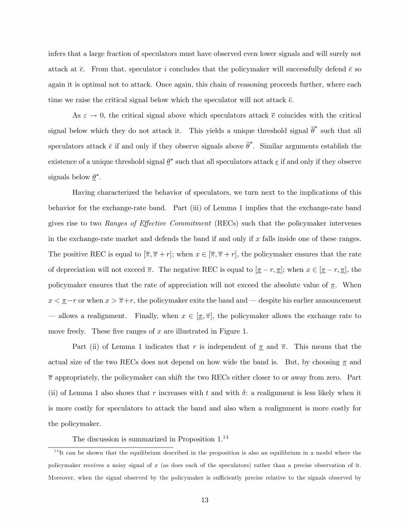
Having characterized the behavior of speculators, we turn next to the implications of this
behavior for the exchange-rate band. Part (iii) of Lemma 1 implies that the exchange-rate band
gives rise to two Ranges of Effective Commitment (RECs) such that the policymaker intervenes
in the exchange-rate market and defends the band if and only if x falls inside one of these ranges.
The positive REC is equal to [π, π + r]; when x ∈ [π, π + r], the policymaker ensures that the rate
of depreciation will not exceed π. The negative REC is equal to [π− r, π]; when x ∈ [π− r, π], the
policymaker ensures that the rate of appreciation will not exceed the absolute value of π. When
x < π−r or when x > π+r, the policymaker exits the band and – despite his earlier announcement
– allows a realignment. Finally, when x ∈ [π, π], the policymaker allows the exchange rate tomove freely. These five ranges of x are illustrated in Figure 1.
Part (ii) of Lemma 1 indicates that r is independent of π and π. This means that the
actual size of the two RECs does not depend on how wide the band is. But, by choosing π and
π appropriately, the policymaker can shift the two RECs either closer to or away from zero. Part
(ii) of Lemma 1 also shows that r increases with t and with δ: a realignment is less likely when it
is more costly for speculators to attack the band and also when a realignment is more costly for
the policymaker.
The discussion is summarized in Proposition 1.14
14 It can be shown that the equilibrium described in the proposition is also an equilibrium in a model where the
policymaker receives a noisy signal of x (as does each of the speculators) rather than a precise observation of it.
Moreover, when the signal observed by the policymaker is sufficiently precise relative to the signals observed by
13
�������������������������������������������������������������������������������������������������������������������������������������������������������������������������������������������������������������
�������������������������������������������������������������������������������������������������������������������������������������������������������������������������������������������������������������
�������������������������������������������������������������������������������������������������������������������������������������������������������������������������������������������������������������Figure 1: Illustrating the exchange rate band����������������������������������������������������������������������������������������������������������������������������������������������������������������������������������������������������������������������������������������������������������������������������������������������������������������������
The positive REC
����������
��������������������
���������������
���������������0
���������
���������x
�������������������������������������������
�������������������������������������������
�������������������������������������������
The negative REC
���������
���������
���������
�������������������������������������������������������������������������������������������������������������
��������������������������������������������������������������������������������������������������
��������������������������������������������������������������������������������������������������No intervention inside the band
���������
���������������������������������������������������������
����
��
��������������
�����������������������������������������������������������
������
����
���������
���������
���������������������������������������������������������������
����������
����������
����������π_
������������������
������������������
������������������π+r_
����������������
��������π_
������������������
������������������
������������������π-r_
��������������������������������������������
��������������������������������������������Realignment
����������
����������������������������������������������������������
�������������������������������������������
�������������������������������������������Realignment
Proposition 1 The exchange-rate band gives rise to a positive range of effective commitment
(REC), [π, π + r], and a negative REC, [π − r, π], where r is defined in Lemma 1.
• When x falls inside the positive (negative) REC, the policymaker defends the currency and
ensures that the maximal rate of depreciation (appreciation) is π (π).
• When x falls below the negative REC, above the positive REC, or inside the band, the policy-
maker lets the exchange rate move freely in accordance with market forces.
• The width of the two RECs, r, increases with t and with δ but is independent of the boundariesof the band, π and π.
3.2 The Choice of Band Width
In order to characterize the equilibrium exchange-rate regime, we first need to write the policy-
maker’s objective function, V (π, π), more explicitly. The first component in V (π, π) represents
the policymaker’s loss from exchange-rate uncertainty. This term depends on the expected rate of
change in the exchange rate, Eπ, which in turn depends on the policymaker’s choices, π and π.
At first blush one may think that, since π is the maximal rate of appreciation and π is
the maximal rate of depreciation, Eπ will necessarily lie between π and π. However, since the
policymaker does not always defend the band, Eπ may in principle fall outside the interval [π, π].
For example, if π is sufficiently small and if f(x) has a larger mass in the positive range of x than
in its negative range, then Eπ will be high. If this asymmetry of f(x) is sufficiently strong, Eπ
will actually be higher than π. Consequently, in writing V (π, π) we need to distinguish between
five possible cases depending on whether Eπ falls inside the interval [π, π], inside one of the two
RECs, below the negative REC, or above the positive REC.
To simplify the exposition, from now on we will restrict attention to the following case:
Assumption 3: The distribution f(x) is symmetric around 0.
Assumption 3 considerably simplifies the following analysis. It implies that the mean of x
is 0 and hence that, on average, the freely floating exchange rate does not generate pressures for
speculators, this equilibrium will be the unique equilibrium, just as in our model.
14
either appreciations or depreciations. We can now prove the following lemma.15
Lemma 2 Given Assumptions 1 and 3, Eπ ∈ [π, π].
Given Lemma 2, the measure of exchange-rate uncertainty is given by:
E |π −Eπ| = −Z π−r
−∞(x−Eπ) dF (x)−
Z π
π−r(π −Eπ) dF (x)−
Z Eπ
π(x−Eπ) dF (x) (4)
+
Z π
Eπ(x−Eπ) dF (x) +
Z π+r
π(π −Eπ)dF (x) +
Z ∞
π+r(x−Eπ)dF (x).
Equation (4) implies that the existence of a band affects uncertainty only through its effect on the
two RECs. Using (1) and (4), the expected payoff of the policymaker, given π and π, becomes
V (π, π) = A
·Z π−r
−∞(x−Eπ)dF (x) +
Z π
π−r(π −Eπ) dF (x) +
Z Eπ
π(x−Eπ) dF (x)
−Z π
Eπ(x−Eπ)dF (x)−
Z π+r
π(π −Eπ) dF (x)−
Z ∞
π+r(x−Eπ) dF (x)
¸(5)
−Z π−r
−∞δdF (x)−
Z π
π−rc(π − x)dF (x)−
Z π+r
πc(x− π)dF (x)−
Z ∞
π+rδdF (x),
where c(·) ≡ C(·, 0). The last line in (5) represents the expected cost of adopting a band. As
Lemma 1 shows, when x falls inside the two RECs, no speculator attacks the band; hence the
policymaker’s cost of intervention in the exchange-rate market is c(π − x) when x ∈ [π − r, π] or
c(x− π) when x ∈ [π, π + r]. When either x < π − r or x > π + r, there are realignments and so
the policymaker incurs a credibility loss δ.
The policymaker chooses the boundaries of the band, π and π, so as to maximize V (π, π).
The next lemma enables us to simplify the characterization of the optimal band.
Lemma 3 Given Assumption 3, the equilibrium exchange-rate band will be symmetric around 0 in
the sense that −π− = π. Consequently, Eπ = 0.
Since the band is symmetric, it is sufficient to characterize the optimal value of the upper
bound of the band, π. By symmetry, the lower bound will then be equal to −π. Given that
15 It should be noted that the general qualitative spirit of our analysis extends to the case where f(x) is asymmetric.
But the various mathematical expressions and conditions become more complex.
15
c(0) ≡ C(0, 0) = 0, it follows that c(r) =R π+rπ c0(x − π)dx. Together with the fact that at the
optimum, Eπ = 0, the derivative of V (π, π) with respect to π is:
∂V (π, π)
∂π= −A
Z π+r
π(f(x)− f(π + r))dx (6)
+
Z π+r
πc0(x− π) (f(x)− f(π + r)) dx+ δf(π + r).
Equation (6) shows that, by altering π, the policymaker trades off the benefits of reducing exchange-
rate uncertainty against the cost of maintaining a band. The term in the first line of (6) is the
marginal effect of π on exchange-rate uncertainty. Since by Assumption 1, f(x) − f(π + r) > 0
for all x ∈ [π, π + r], this term is negative and represents the marginal cost of raising π. This
marginal cost arises because, when π is raised, the positive REC over which the exchange rate is
kept constant shifts farther away from the center rate to a range of shocks that is less likely (by
Assumption 1). Hence, the band becomes less effective in reducing exchange-rate uncertainty.
The second line in (6) represents the marginal effect of raising π on the expected cost of adopting
a band. By Assumption 1 and since c0(·) > 0, the integral term is positive, implying that raising πmakes it less costly to defend the band. This is because it is now less likely that the policymaker
will actually have to defend the band. The term involving δ is also positive since increasing π
slightly lowers the likelihood that the exchange rate will move outside the positive REC and lead
to a realignment.
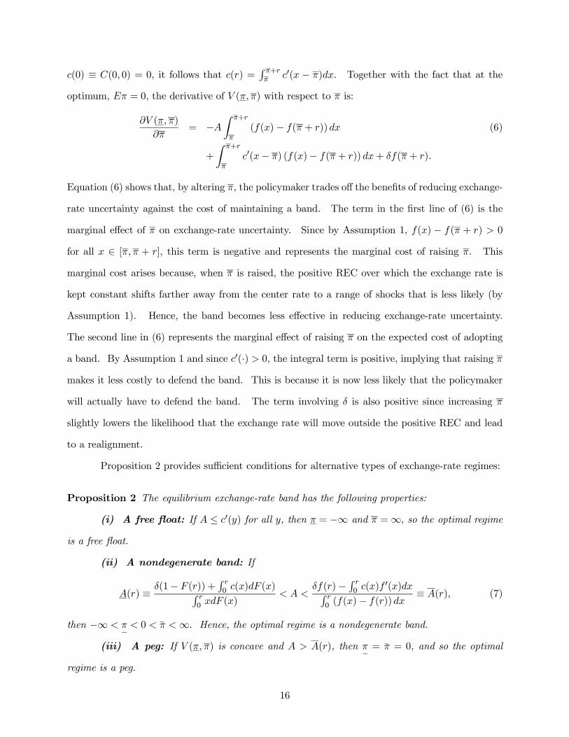
Proposition 2 provides sufficient conditions for alternative types of exchange-rate regimes:
Proposition 2 The equilibrium exchange-rate band has the following properties:
(i) A free float: If A ≤ c0(y) for all y, then π = −∞ and π =∞, so the optimal regime
is a free float.
(ii) A nondegenerate band: If
A(r) ≡ δ(1− F (r)) +R r0 c(x)dF (x)R r
0 xdF (x)< A <
δf(r)− R r0 c(x)f 0(x)dxR r0 (f(x)− f(r))dx
≡ A(r), (7)
then −∞ < π− < 0 <_π <∞. Hence, the optimal regime is a nondegenerate band.
(iii) A peg: If V (π, π) is concave and A > A(r), then π− =_π = 0, and so the optimal
regime is a peg.
16
Part (i) of Proposition 2 states that when the policymaker has sufficiently little concern
for nominal exchange-rate uncertainty (i.e., A is small relative to c0(y)), then he sets a free float
and completely avoids the cost of maintaining a band. Part (ii) of the proposition identifies an
intermediate range of values of A for which the optimal regime is a nondegenerate band. When
A is below the upper bound of this range, A(r), it is optimal to increase π above zero and thus
the optimal regime is not a peg. When A is above the lower bound of this range, A(r), a peg is
better than a free float. Thus, when A is inside this range, the optimal regime is a nondegenerate
band.16 Part (iii) of Proposition 2 states that if the policymaker is highly concerned with nominal
exchange-rate uncertainty (i.e., A > A(r)), then his best strategy is to adopt a peg.17
4 Comparative Statics and Empirical Implications
In this section, we examine the comparative statics properties of the optimal band under the
assumption that there is an internal solution (i.e., the optimal regime is a non-degenerate band).
This means that the solution is obtained by equating the expression in (6) to zero. To assure that
such a solution exists, we assume that A > c0(y) for all y. In the appendix, we derive conditions
for a unique internal solution.
4.1 The Effects of Restrictions on Capital Flows and of a Tobin Tax
During the last three decades there has been a worldwide gradual lifting of restrictions on currency
flows and on related capital account transactions. One consequence of this trend is a reduction
in the transaction cost of foreign exchange transactions (t in terms of the model), making it easier
16Note that the range specified in equation (7) represents only a (restrictive) sufficient condition for the optimal
regime to be a nondegenerate band. Thus, the actual range in which the regime is a nondegenerate band should
be larger. Also, note that the range in (7) is usually nonempty. For example, when C(y, α) = y + α and f(x) is
a triangular symmetric distribution function with supports −x and x (x > 0), this range is nonempty for all r < x.
For brevity, we do not demonstrate this explicitly in the paper.17Note that a peg does not mean that the exchange rate is fixed under all circumstances. When the absolute
value of x exceeds r, the policymaker abandons the peg and the exchange rate is realigned. Hence, under a peg, the
exchange rate is fixed for all x ∈ [−r, r]. Given Assumption 1, such “small” shocks are more likely than big ones, sowhen A is large it is optimal for the policymaker to eliminate these shocks by adopting a peg.
17
for speculators to move funds across different currencies and thereby facilitating speculative at-
tacks. To counteract this tendency, some economists proposed to “throw sand” into the wheels of
unrestricted international capital flows. In particular, Tobin (1978) proposed a universal tax on
short-term intercurrency transactions in order to reduce the profitability of speculation against the
currency and hence the probability of crises. This idea was met with skepticism owing mainly to
difficulties of implementation. Yet, by and large the consensus is that, subject to feasibility, the tax
can reduce the probability of attack on the currency. Recent evaluations appear in Eichengreen,
Tobin and Wyplosz (1995), Jeanne (1996), Haq, Kaul and Grunberg (1996), Eichengreen (1999),
and Berglund et al. (2001).
The main objective of this section is to examine the consequences of such a tax and of the
lifting of restrictions on capital flows when the choice of exchange-rate regime is endogenous.
Proposition 3 Suppose that, following a lifting of restrictions on currency flows and capital ac-
count transactions, the transaction cost of switching between currencies, t, decreases. Then:
(i) When the policymaker’s problem has a unique interior solution,_π and π− shift away from zero
and so the band becomes wider. Moreover, the probability, P , that a speculative attack occurs
decreases.
(ii) The bound A(r), above which the policymaker adopts a peg, increases, implying that policy-
makers adopt pegs for a narrower range of values of A.
(iii) The equilibrium value of the policymaker’s objective, V , falls.
Part (i) of Proposition 3 states that lifting restrictions on the free flow of capital induces
policymakers to pursue less ambitious stabilization objectives by allowing the exchange rate to
move freely within a wider band. This result is consistent with the flexibilization of exchange-rate
regimes following the gradual elimination of restrictions on capital flows in the aftermath of the
Bretton Woods system. Moreover, the proposition states that this reduction in transaction costs
lowers, on balance, the likelihood of a currency crisis. This result reflects the operation of two
opposing effects. First, as Proposition 1 shows, the two RECs shrink when t decreases. Holding
18
the band width constant, this raises the probability of speculative attacks. This effect already
appears in the literature on international financial crises (e.g., Morris and Shin 1998). But, as
argued above, following the decrease in t, the band becomes wider, and this lowers, in turn, the
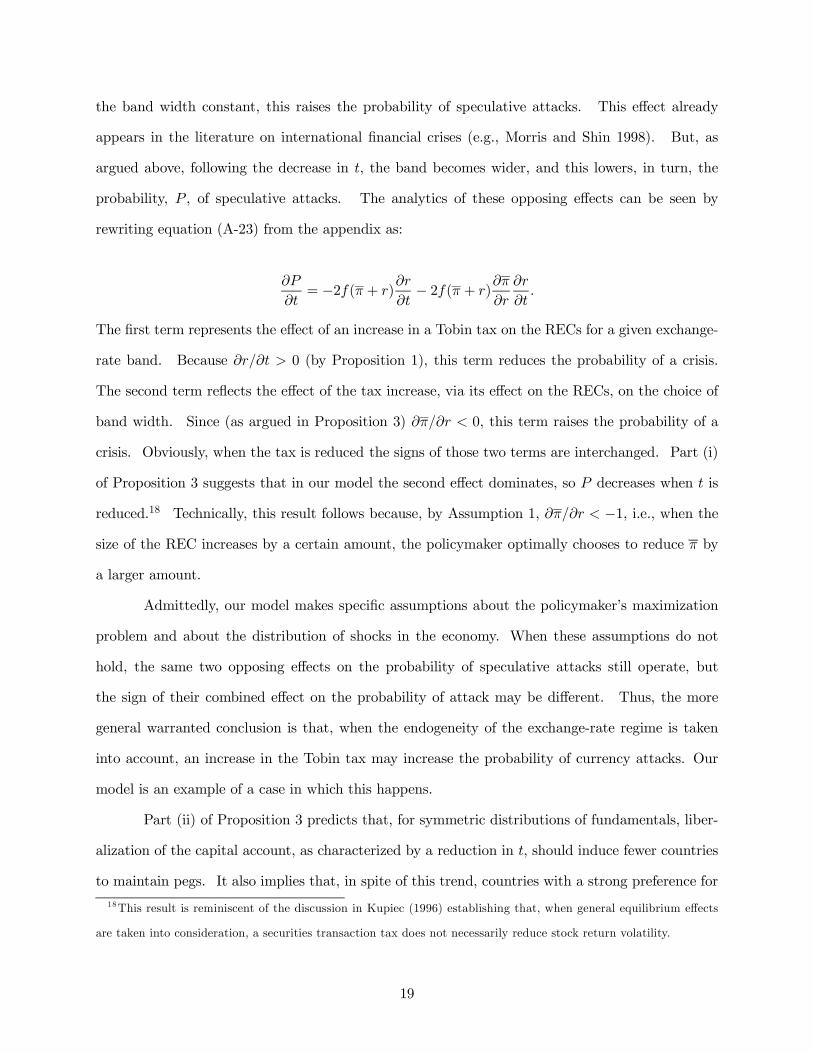
probability, P , of speculative attacks. The analytics of these opposing effects can be seen by
rewriting equation (A-23) from the appendix as:
∂P
∂t= −2f(π + r)
∂r
∂t− 2f(π + r)
∂π
∂r
∂r
∂t.
The first term represents the effect of an increase in a Tobin tax on the RECs for a given exchange-
rate band. Because ∂r/∂t > 0 (by Proposition 1), this term reduces the probability of a crisis.
The second term reflects the effect of the tax increase, via its effect on the RECs, on the choice of
band width. Since (as argued in Proposition 3) ∂π/∂r < 0, this term raises the probability of a
crisis. Obviously, when the tax is reduced the signs of those two terms are interchanged. Part (i)
of Proposition 3 suggests that in our model the second effect dominates, so P decreases when t is
reduced.18 Technically, this result follows because, by Assumption 1, ∂π/∂r < −1, i.e., when thesize of the REC increases by a certain amount, the policymaker optimally chooses to reduce π by
a larger amount.
Admittedly, our model makes specific assumptions about the policymaker’s maximization
problem and about the distribution of shocks in the economy. When these assumptions do not
hold, the same two opposing effects on the probability of speculative attacks still operate, but
the sign of their combined effect on the probability of attack may be different. Thus, the more
general warranted conclusion is that, when the endogeneity of the exchange-rate regime is taken
into account, an increase in the Tobin tax may increase the probability of currency attacks. Our
model is an example of a case in which this happens.
Part (ii) of Proposition 3 predicts that, for symmetric distributions of fundamentals, liber-
alization of the capital account, as characterized by a reduction in t, should induce fewer countries
to maintain pegs. It also implies that, in spite of this trend, countries with a strong preference for
18This result is reminiscent of the discussion in Kupiec (1996) establishing that, when general equilibrium effects
are taken into consideration, a securities transaction tax does not necessarily reduce stock return volatility.
19
exchange-rate stability (e.g., small open economies with relatively large shares of foreign currency
denominated trade and capital flows as well as emerging markets) will continue to peg even in
the face of capital market liberalization. In contrast, countries with intermediate preferences for
exchange-rate stability (e.g., more financially mature economies with a larger fraction of domesti-
cally denominated debt and capital flows) will move from pegs to bands. These predictions seem
to be consistent with casual evidence. Two years following the 1997—1998 East Asian crisis, most
emerging markets countries in that region were back on pegs (McKinnon 2001; Calvo and Reinhart
2002). On the other hand, following the EMS currency crisis at the beginning of the 1990s, the
prior system of cooperative pegs was replaced by wide bands until the formation of the EMU at
the beginning of 1999.
Finally, part (iii) of Proposition 3 shows that, although a decrease in t lowers the likelihood
of a financial crisis, it nonetheless makes the policymaker worse off. The reason is that speculative
attacks impose a constraint on the policymaker when choosing the optimal exchange-rate regime. A
decrease in t strengthens the incentive to mount a speculative attack and thus makes this constraint
more binding.
Importantly, the conception underlying the analysis here is that a Tobin tax as originally
conceived by Tobin, is imposed only on short-term speculative trading and not on current account
transactions and long-term capital flows.19 Hence it affects short-term speculative trading, and
through it government intervention, but not current account transactions and long-term capital
flows, whose impact on the exchange rate is modeled by means of the exogenous stochastic variable
x. For realizations of x outside the band and a given exchange-rate regime, the model captures
the fact that a Tobin tax reduces speculative trading and causes the actual exchange rate to be
closer on average to the boundaries of the band via the, endogenous, behavior of π.
19We abstract from some of the practical difficulties involved in distinguishing between short-term speculative flows
and longer-term capital flows.
20
4.2 The Effects of Intensity of Aversion to Exchange-Rate Uncertainty
We now turn to the effects of the parameter A (the relative importance that the policymaker assigns
to reduction of exchange-rate uncertainty) on the choice of regime. As argued above, in small open
economies with large fractions of assets and liabilities denominated in foreign exchange, residents
are more averse to nominal exchange-rate uncertainty than residents of large, relatively closed
economies, whose financial assets and liabilities are more likely to be denominated in domestic
currency. Hence the parameter A reflects the size of the economy and the degree to which it is
open, with larger values of A being associated with smaller and more open economies.
Proposition 4 Suppose that the policymaker’s problem has a unique interior solution. Then, as
A increases (the policymaker becomes more concerned with exchange rate stability):
(i)_π and π− shift closer to zero, so the band becomes tighter; and
(ii) the probability, P , that a speculative attack will occur increases.
Proposition 4 states that, as the policymaker becomes more concerned with reduction of
uncertainty, he sets a tighter band and allows the exchange rate to move freely only within a
narrower range around the center rate.20 Part (ii) of the proposition shows that this tightening of
the band raises the likelihood of a speculative attack. This implies that, all else equal, policymakers
in countries with larger values of A are willing to set tighter bands and face a higher likelihood of
speculative attacks than policymakers in otherwise similar countries with lower values of A.
Note that as Proposition 2 shows, when A increases above A(r), the optimal band width
becomes zero and so the optimal regime is a peg. On the other hand, when A falls and becomes
smaller than c0(·), the optimal band width becomes infinite, and so the optimal regime is a freefloat. Given that a substantial part of international trade is invoiced in U.S. Dollars (McKinnon
1979), it is likely that policymakers of a key currency country like the United States will be less
sensitive to nominal exchange-rate uncertainty and therefore have a smaller A than policymakers in
20This result may appear obvious at first blush. But the fact that it obtains only under unimodality (Assumption
1) suggests that such preliminary intuition is incomplete in the absence of suitable restrictions on the distribution of
fundamentals.
21
small open economies. Therefore, our model predicts that the United States, Japan, and the Euro
area should be floating, whereas Hong Kong, Panama, Estonia, Lithuania, and Bulgaria should be
on either pegs, currency boards, or even full dollarization. This prediction appears to be consistent
with casual observation of the exchange-rate systems chosen by those countries.
4.3 The Effects of Increased Variability in Fundamentals
Next, we examine how the exchange-rate band changes when more extreme realizations of x become
more likely. This comparative statics exercise involves shifting probability mass from moderate
realizations of x that do not lead to realignments to more extreme realizations that do lead to
realignments.
Proposition 5 Suppose that the policymaker’s problem has a unique interior solution. Also sup-
pose that f(x) and g(x) are two symmetric density functions with a mode (and a mean) at zero
such that
(i) g(x) lies below f(x) for all π − r < x <_π + r, and
(ii) g(_π + r) = f(
_π + r) and g(π − r) = f(π − r),
where π and_π are the solutions to the policymaker’s problem under the original density function
f(x) (i.e., g(x) has fatter tails than f(x)). Then, the policymaker adopts a wider band under g(x)
than under f(x).
Intuitively, as more extreme realizations of x become more likely (the density f(x) is replaced
by g(x)), the policymaker is more likely to incur the loss of future credibility associated with
realignments. Therefore, the policymaker widens the band to offset the increase in the probability
that a costly realignment will take place. In addition, as larger shocks become more likely, the
policymaker also finds it optimal to shift the two RECs further away from zero in order to shift his
commitment to intervene in the market to a range of shocks that are now more probable. This
move benefits the policymaker’s objectives by counteracting part of the increased uncertainty about
the freely floating value of the exchange rate. Both factors induce a widening of the band.
22
4.4 The Effects of Tightness of Commitment to Maintaining the Regime
The degree of commitment to the exchange-rate regime is represented in our model by the parameter
δ. Using the assumption that f(x) is symmetric (in which case Eπ = 0) and totally differentiating
equation (6) with respect to δ reveals that, in general, δ has an ambiguous effect on the optimal
width of the band. On one hand, Proposition 1 implies that the width of the two RECs, r,
increases as δ increases. This is because – given the width of the band – speculators are less
likely to attack the band when they know that the policymaker is more likely to defend it. This
reduced likelihood of attacks induces the policymaker to set a narrower band. On the other hand,
as δ increases, the cost of realignments (when they occur) increases because they lead to a larger
credibility loss. This effect pushes the policymaker to widen the band. Overall, then, the width
of the band may either increase or decrease with δ.
Since the probability of speculative attack, P , is affected by the width of the band, the
effect of δ on P is also ambiguous. For a given regime, Proposition 1 implies that P decreases with
δ (since speculators are less likely to attack when they know that the policymaker is more likely to
defend a given band). However, when the endogeneity of the regime is recognized, the discussion
in the previous paragraph implies that this result may be reversed. In particular, when δ increases
the policymaker may decide to narrow the band since he knows that, given the width of the band,
he will subsequently decide to maintain the regime for a larger set of values of x. This, in turn,
may increase the ex ante probability of a speculative attack. Consequently, an increase in the
tightness of commitment may increase the probability of speculative attack.21
5 Concluding Reflections
This paper develops a framework for analyzing the interaction between the ex ante choice of
exchange-rate regime and the probability of ex post currency attacks. To the best of our knowl-
21We also tried to characterize the optimal degree of commitment to the regime but, since the ratio of economic
insights to algebra was low, this experiment is not presented. Cukierman, Kiguel and Liviatan (1992) and Flood
and Marion (1999) present such an analysis for exogenously given pegs. The analysis here is more complex owing to
the fact that it involves the simultaneous choice of the band width and the degree of commitment.
23
edge, this is the first paper that solves endogenously for the optimal regime and for the probability
of currency attacks and studies their interrelation.
Our framework generates several novel predictions that are consistent with empirical ev-
idence. First, we find that financial liberalization that lowers the transaction costs of switching
between currencies induces the policymaker to adopt a more flexible exchange-rate regime. This is
broadly consistent with the flexibilization of exchange-rate regimes following the gradual reductions
of restrictions on capital flows in the aftermath of the Bretton Woods system (Isard 1995). Second,
in our model, small open economies with substantial aversion to exchange-rate uncertainty are
predicted to have narrower bands and more frequent currency attacks than large, relatively closed
economies. This is broadly consistent with the fact that large economies with key currencies – such
as the United States, Japan, and the Euro area – choose to float, while small open economies like
Argentina (until the beginning of 2002), Thailand, and Korea choose less flexible regimes that are
more susceptible to currency attacks like the 1997—1998 Southeast Asian crisis. In a wider sense,
the paper suggests that a higher risk of currency attack is the price that small open economies are
willing to pay for smaller exchange-rate uncertainty. Third, we show that increased variability in
fundamentals generates wider bands.
Another prediction of the model, not highlighted so far, is related to the bipolar view.
According to this hypothesis, in the course of globalization there has been a gradual shift away
from intermediate exchange-rate regimes to either hard pegs or freely floating regimes (Fischer
2001). Globalization is expected to have two opposite effects in our model. On one hand, it
lowers the cost of switching between currencies and hence facilitates speculation; this effect induces
policymakers to set more flexible regimes. On the other hand, globalization increases the volume
of international trade in goods and financial assets, thereby increasing the aversion to nominal
exchange-rate uncertainty; this effect induces policymakers to set less flexible regimes. The second
effect is likely to be large for small open economies whose currencies are not used much for either
capital account or current account transaction in world markets, and to be small or even negligible
for large key currency economies. Hence, the first effect is likely to be dominant in large, relatively
closed blocks while the second is likely to dominate in small open economies. All else equal, the
24
process of globalization should therefore induce relatively large currency blocks to move toward more
flexible exchange-rate arrangements while pushing small open economies in the opposite direction.
Another result of our model is that a Tobin tax raises the probability of currency attacks.
Although (as in existing literature) a Tobin tax reduces the probability of a currency attack for a
given exchange-rate regime, the analysis also implies that the tax induces policymakers to set less
flexible regimes. Hence, once the choice of an exchange-rate regime is endogenized, the tax has an
additional, indirect, effect on the likelihood of a currency attack. In our model, this latter effect
dominates the direct effect. Similarly, our model suggests that the effect of a larger credibility loss
– following a realignment – on the probability of speculative attacks is ambiguous. For a given
regime, when this credibility loss is higher, policymakers have a stronger incentive to defend the
exchange-rate regime against speculative attacks, and this lowers the probability of such an event.
However, once the choice of a regime is endogenized, the overall effect becomes ambiguous since ex
ante, realizing that speculative attacks are less likely, policymakers may have an incentive to adopt
a less flexible regime.
The model can be extended to allow for imperfect information on the part of the public
about the commitment ability of policymakers. In such a framework there are two types of
policymaker: a dependable type – who is identical to the one considered in this paper – and an
opportunistic type, for whom the personal cost of realignment (perhaps due to a high degree of,
politically motivated, positive time preference) is zero. The latter type lets the exchange rate float
ex post for all realizations of fundamentals. As in Barro (1986), the probability assigned by the
public to a dependable type being in office is taken as a measure of reputation. The model in this
paper obtains as a particular case of the extended case when reputation is perfect. The extended
analysis appears in Cukierman, Goldstein and Spiegel (2003, Section 5) and is not presented here
for the sake of brevity.
An interesting implication of the extended framework is that policymakers with high repu-
tation tend to set less flexible regimes and are less vulnerable to speculative attacks. Hong Kong’s
currency board is a good example. Because it has never abandoned its currency board in the
past, Hong-Kong’s currency board enjoys a good reputation and attracts less speculative pressure.
25
Another implication of the extended framework is that the width of the REC’s is an increasing
function of reputation, which provides an explanation for the triggers of some crises like the 1994
Mexican crisis or the 1992 flight from the French Franc following the rejection of the Maastricht
Treaty by Danish voters.22
Although our framework captures many empirical regularities regarding exchange-rate regimes
and speculative attacks, it obviously does not capture all of them. For example, as Calvo and Rein-
hart (2002) have shown, policymakers often intervene in exchange-rate markets even in the absence
of explicit pegs or bands. We believe that an extension analyzing the desirability of implicit bands
(as well as other regimes is) a promising direction for future research.23 Another such direction is
the development of a dynamic framework in which the fundamentals are changing over time and
speculators can attack the currency at several points in time. The optimal policy in a dynamic
context raises additional interesting issues, such as changes in the policymaker’s reputation over
time.
6 Appendix
Proof of Lemma 1: (i) We analyze the behavior of the policymaker and the speculators after
the exchange rate reaches the upper bound of the band. We show that as ε → 0, there exists a
22Prior to the Mexican crisis, Mexico maintained a peg for several years and had, therefore, good reputation.
When the ruling party’s presidential candidate, Colosio, was assassinated in March 1994, the Mexican Peso came
under attack. The authorities defended the Peso initially but, following a substantial loss of reserves within a short
period of time, allowed it to float. The extended framework provides an explanation for the crisis within a unique
equilibrium framework. Prior to Colosio’s assassination, fundamentals were already stretched so that, in the absence
of intervention, the Peso would have depreciated. But, since reputation was high, speculators anticipated that the
Mexican government would defend the peg for the existing range of realizations of x and thus refrained from attacking
it. The assassination and the subsequent political instability led to an abrupt decrease in reputation, narrowing the
RECs around the Mexican peg and creating a new situation in which the free market rate, x, fell outside the positive
REC. It then became rational for speculators to run on the Peso and for the Mexican government not to defend it.
A similar explanation can be applied to the Danish episode described in Isard (1995, p. 210).
23A theoretical discussion of implicit bands appears in Koren (2000). See also Bartolini and Prati (1999).
26
unique perfect Bayesian equilibrium in which each speculator i attacks the band if and only if θi
is above a unique threshold θ∗. The proof for the case where the exchange rate reaches the lower
bound of the band is analogous.
We start with some notation. First, suppose that x ≥ π and let α∗ (x) be the critical
measure of speculators below which the policymaker defends the upper bound of the band when
the laissez-faire rate of change in the exchange rate is x. Recalling that the policymaker defends
the band if and only if C(y, α) ≤ δ, and using the fact that y = x− π, α∗ (x) is defined implicitly
by
C(x− π, α∗(x)) = δ. (A-1)
Since C(x− π, α∗(x)) increases with both arguments, dα∗ (x) /dx ≤ 0.Then, the net payoff from attacking the upper bound of the band is:
v(x, α) =
(x− π) e−1 − t, if α > α∗ (x) ,
−t, if α ≤ α∗ (x) .(A-2)
Note that ∂v(x, α)/∂α ≥ 0 because the assumption that x ≥ π implies that the top line in (A-
2) exceeds the bottom line. Moreover, noting from (A-1) that dα∗ (x) /dx ≤ 0, it follows that∂v(x,α)/∂x ≥ 0 with a strict inequality whenever v(x, α) ≥ 0.
Let αi(x) be speculator i’s belief about the measure of speculators who will attack the band
for each level of x. We will say that the belief bαi(·) is higher than αi(·) if bαi(·) ≥ αi(·) for all xwith strict inequality for at least one x.
The decision of speculator i whether or not to attack e depends on the signal θi that
speculator i observes and his belief, αi(·). Using (3), the net expected payoff of speculator i fromattacking e is:
h(θi, αi(·)) =Z θi+ε
θi−εv(x, αi(x))f(x | θi)dx =
R θi+εθi−ε v(x, αi(x))f(x)dxF (θi + ε)− F (θi − ε)
. (A-3)
We now establish three properties of h(θi, αi(·)):
Property 1: h(θi, αi(·)) is continuous in θi.
Property 2: bαi(·) ≥ αi(·) implies that h(θi, bαi(·)) ≥ h(θi, αi(·)) for all θi.
27
Property 3: ∂h(θi, αi(·))/∂θi ≥ 0 if αi(·) is nondecreasing in x with strict inequality whenever
h(θi, αi(·)) ≥ 0.
Property 1 follows because F (·) is a continuous function. Property 2 follows because
∂v(x,α)/∂α ≥ 0. To establish Property 3, note that
∂h(θi, αi(·))∂θi
=[v (θi + ε, αi(θi + ε)) f(θi + ε)− v (θi − ε, αi(θi − ε)) f(θi − ε)]
R θi+εθi−ε f(x)dx
(F (θi + ε)− F (θi − ε))2
− [f(θi + ε)− f(θi − ε)]R θi+εθi−ε v(x,αi(x))f(x)dx
(F (θi + ε)− F (θi − ε))2(A-4)
=f(θi + ε)
R θi+εθi−ε [v (θi + ε, αi(θi + ε))− v(x,αi(x))] f(x)dx
(F (θi + ε)− F (θi − ε))2
+f(θi − ε)
R θi+εθi−ε [v(x, αi(x))− v (θi − ε, αi(θi − ε))] f(x)dx
(F (θi + ε)− F (θi − ε))2.
Recalling that ∂v(x, α)/∂x ≥ 0 and ∂v(x,α)/∂α ≥ 0, it follows that ∂h(θi, αi(·))/∂θi ≥ 0 if αi(·) isnondecreasing in x. Moreover, (A-3) implies that if h(θi, αi(·)) ≥ 0, then there exists at least onex ∈ [θi − ε, θi + ε] for which v(x,αi(·)) > 0 (otherwise, h(θi, αi(·)) < 0). Since ∂v(x,α)/∂x > 0 if
v(x,α) ≥ 0, it follows in turn that ∂v(x, α)/∂x > 0 for at least one x ∈ [θi − ε, θi + ε]. But since
∂v(x,α)/∂x ≥ 0 with strict inequality for at least one x, (A-4) implies that ∂h(θi, αi(·))/∂θi > 0
whenever h(θi, αi(·)) ≥ 0.In equilibrium, the strategy of speculator i is to attack e if h(θi, αi(·)) > 0 and not attack it
if h(θi, αi(·)) < 0. Moreover, the equilibrium belief of speculator i, αi(·), must be consistent withthe equilibrium strategies of all other speculators (for short we will simply say that, in equilibrium,
“the belief of speculator i is consistent”). To characterize the equilibrium strategies of speculators,
we first show that there exists a range of sufficiently large signals for which speculators have a
dominant strategy to attack e and, likewise, there exists a range of sufficiently small signals for
which speculators have a dominant strategy not to attack e. Then, we use an iterative process
of elimination of dominated strategies to establish the existence of a unique signal, θ∗, such that
speculator i attacks e if and only if θi > θ∗.
Suppose that speculator i observes a signal θi > θ, where θ is defined by the equation
C¡¡θ − π − ε
¢, 0¢= δ. Then speculator i realizes that the policymaker is surely going to exit
28
the band. By (A-2), the net payoff from attacking e is therefore v(x,α) = (x − π)e−1 − t, for all
α. From Assumption 2, it follows that v(x, α) is strictly positive within the range [θi − ε, θi + ε].
Hence, by (A-3), h(θi, αi(x)) > 0 for all θi > θ and all αi(x), implying that it is a dominant
strategy for speculator i with θi > θ to attack e. Similarly, if θi < θ, where θ ≡ π + t/e−1 − ε
(since we focus on the case where ε→ 0 and since t > 0, such signals are observed with a positive
probability whenever x > π), speculator i realizes that x < π + t/e−1. Consequently, even if the
policymaker surely exits the band, the payoff from attacking it is negative. This implies in turn
that h(θi, αi(x)) < 0 for all θi < θ and all αi(x), so it is a dominant strategy for speculator i with
θi < θ not to attack.
Now, we start an iterative process of elimination of dominated strategies from θ in order
to expand the range of signals for which speculators will surely attack e. To this end, let α(x, θ)
represent a speculator’s belief regarding the measure of speculators who will attack e for each level
of x, when the speculator believes that all speculators will attack e if and only if their signals are
above some threshold θ. Since εi ∼ U [−ε, ε],
α(x, θ) =
0, if x < θ − ε,
x−(θ−ε)2ε , if θ − ε ≤ x ≤ θ + ε,
1, if x > θ + ε.
(A-5)
The iterative process of elimination of dominated strategies works as follows. We have already
established that h(θi, αi(x)) > 0 for all θi > θ and all αi(x). But since h(θi, αi(x)) is continuous
in θi, it follows that h(θ, αi(x)) ≥ 0 for all αi(x) and in particular for αi(x) = α(x, θ). Thus,
h(θ, α(x, θ)) ≥ 0. Note that since in equilibrium the beliefs of speculators are consistent, only
beliefs that are higher than or equal to α(x, θ) can hold in equilibrium (because all speculators
attack e when they observe signals above θ). Thus, we say that α(x, θ) is the “lowest” consistent
belief on α.
Let θ1be the value of θi for which h(θi, α(x, θ)) = 0. That is, h(θ
1, α(x, θ)) ≡ 0. Note
that θ1 ≤ θ, and that θ
1is defined uniquely because we showed above that h(θi, αi(x)) is strictly
increasing in θi whenever h(θi, αi(x)) ≥ 0. Using Properties 2 and 3 and recalling that α(x, θ) isthe lowest consistent belief on α, it follows that h(θi, αi(x)) > 0 for any θi > θ
1and any consistent
29
belief αi(x). Thus, in equilibrium, speculators must attack e if they observe signals above θ1. As
a result, α(x, θ1) becomes the lowest consistent belief on αi(x).
Starting from θ1, we can now repeat the process along the following steps (these steps
are similar to the ones used to establish θ1). First, note that since h(θ
1, α(x, θ)) ≡ 0 and since
α(x, θ) is weakly decreasing with θ and h(θi, αi(x)) is weakly increasing with αi(x), it follows that
h(θ1, α(x, θ
1)) ≥ 0. Second, find a θi ≤ θ
1for which h(θi, α(x, θ
1)) = 0 and denote it by θ
2.
Using the same arguments as above, θ2is defined uniquely. Third, since α(x, θ
1) is the lowest
consistent belief on αi(x) and using the second and third properties of h(θi, αi(x)), it follows that
speculators must attack e if they observe signals above θ2. The lowest possible belief on αi(x)
becomes α(x, θ2).
We repeat this process over and over again (each time lowering the value of θ above which
speculators will attack e), until we reach a step n such that θn+1
= θn, implying that the process
cannot continue further. Let θ∞denote the value of θ at which the process stops. (Clearly,
θ∞ ≤ θ.) By definition, speculators will attack e if they observe signals above θ
∞. Since θ
∞is the
point where the process stops, it must be the case that h(θ∞, α(x, θ
∞)) = 0 (otherwise, we could
find some θi < θ∞for which h(θi, α(x, θ
∞)) = 0, meaning that the iterative process could have
been continued further).
Starting a similar iterative process from θ and following the exact same steps, we also obtain
a signal θ∞ (≥ θ) such that speculators will never attack e if they observe signals below or at θ∞
(strictly speaking, at this signal the speculator is indifferent between attacking and not attacking;
we break the tie by assuming that, when indifferent, the speculator chooses not to attack). At
this signal, it must be the case that h(θ∞, α(x, θ∞)) = 0. Since we proved that in equilibrium
speculators attack e if they observe signals above θ∞and do not attack it if they observe signals
below θ∞, it must be the case that θ∞ ≥ θ∞.
The last step of the proof involves showing that θ∞= θ∞ as ε→ 0. First, recall that θ
∞
is defined implicitly by h(θ∞, α(x, θ
∞)) = 0. Using (A-3) and (A-5), this equality can be written
30
as R θ∞+εθ∞−ε v
³x, x−(θ
∞−ε)2ε
´f(x)dx
F³θ∞+ ε´− F
³θ∞ − ε
´ = 0. (A-6)
Using the equality α =³x− (θ∞ − ε)
´/2ε to change variables in the integration, (A-6) can be
written as:
2εR 10 v(θ
∞+ 2εα− ε, α)f(θ
∞+ 2εα− ε)dα
F³θ∞+ ε´− F
³θ∞ − ε
´ (A-7)
=
R 10 v(θ
∞+ 2εα− ε, α)f(θ
∞+ 2εα− ε)dα
F(θ∞+ε)−F(θ∞−ε)
2ε
= 0.
As ε → 0, this equation becomesR 10 v(θ
∞, α)dα = 0 (by L’Hôpital’s rule, the denominator ap-
proaches f³θ∞´
as ε → 0). Likewise, as ε → 0, θ∞ is defined implicitly byR 10 v(θ
∞, α)dα = 0.
Now, assume by way of negation that θ∞
> θ∞. Since ∂v(x,α)/∂x ≥ 0 with a strict inequalitywhen v(x,α) ≥ 0, it follows that R 10 v(θ∞, α)dα >
R 10 v(θ
∞, α)dα (the strict inequality follows be-
causeR 10 v(θ
∞, α)dα = 0 implies that v(θ
∞, α) > 0 for at least some values of α). This inequality
contradicts the fact thatR 10 v(θ
∞, α)dα = 0 and
R 10 v(θ
∞, α)dα = 0.
Using the notation θ∗ ≡ θ
∞= θ∞, we proved that as ε→ 0, there exists a unique threshold
signal, θ∗, such that all speculators will attack e if and only if they observe signals above θ
∗.
(ii)We now characterize θ∗; the characterization of θ∗ is then completely analogous. Given
x and θ∗, the measure of speculators who choose to attack e is α(x, θ
∗), where α(x, θ
∗) is defined
in (A-5). Now recall that the policymaker exits the band if C (x− π,α) > δ. Given α(x, θ∗), a
realignment takes place if and only if C³x− π,α(x, θ
∗)´> δ. Since α(x, θ
∗) is weakly increasing
in x, a realignment takes place if and only if x is above some threshold x(θ∗).
Note that, in a perfect Bayesian equilibrium, we cannot have x(θ∗) < θ
∗ − ε. This can be
proved by establishing a contradiction. Suppose by way of negation that x(θ∗) < θ
∗− ε. Then, at
the signal θ∗, a speculator knows that the government abandons the band. By the definition of θ
∗,
the speculator is indifferent between attacking the band and not attacking it. Thus, it must be the
case that when the fundamentals are at the lowest possible level given signal θ∗, the speculator gets
a negative profit from attacking, i.e., θ∗−ε < π+t/e−1. This implies that x(θ
∗) < π+t/e−1. Since
the policymaker is indifferent between attacking or not at x(θ∗), and since C (x− π,α) is increasing
31
in both arguments, this implies that C (t/e−1, 0) > δ, which is a contradiction to Assumption 2.
Similarly, one can show that we cannot have x(θ∗) > θ
∗+ ε. Hence, in equilibrium we must have
θ∗− ε ≤ x(θ
∗) ≤ θ
∗+ ε. Let α∗ be the proportion of agents who attack the currency at x(θ∗); this
proportion is defined implicitly by:
C³x(θ
∗)− π,α∗
´= δ. (A-8)
Next, consider the decision problem that speculator i faces after observing the signal θi.
Given that θi is drawn from the interval [x− ε, x+ ε] , speculator i realizes that x is distributed
on the interval [θi − ε, θi + ε] , and its conditional density is given by (3). But, since speculator
i anticipates that the policymaker will defend e whenever x < x(θ∗), he expects a net payoff of
(x−π)e−1− t if x > x(θ∗) or of −t if x < x(θ
∗). Part (i) of the lemma implies that, in equilibrium,
speculators attack e if and only if they observe signals above θ∗. A speculator who observes exactly
θ∗is indifferent between attacking and not attacking. Using this indifference condition, we obtain,Z θ
∗+ε
x(θ∗)(x− π)e−1f(x | θ∗)dx− t = 0. (A-9)
Substituting for f(x | ·) from (3) into (A-9) and taking the limit as ε→ 0, results in:
limε→0
R θ∗+εx(θ
∗)(x− π)e−1f(x)dx
F³θ∗+ ε´− F
³θ∗ − ε
´ = t.
Changing the variable of integration to α, and using (A-8), we get:
limε→0
2εR 1α∗(2εα+ θ
∗ − ε− π)f(2εα+ θ∗ − ε)dα
F³θ∗+ ε´− F
³θ∗ − ε
´ =t
e−1.
Using L’Hôpital’s rule, and noting that x³θ∗´ → θ
∗as ε → 0, the left-hand side of this equation
becomes Z 1
α∗(θ∗ − π)dα = r (1− α∗) , (A-10)
where r ≡ θ∗ − π. Hence,
r (1− α∗) =t
e−1. (A-11)
In addition, since x³θ∗´→ θ
∗as ε→ 0, (A-8) becomes
C (r, α∗) = δ. (A-12)
32
Substituting for α∗ from (A-11) into (A-12) yields the expression that appears in the propo-
sition and implicitly defines r. Recalling that C(·, ·) is increasing in both of its arguments, it iseasy to verify from these two equations that r is increasing in t and in δ and is independent of π.
Note also that r has to be positive. This is because θ∗ ≥ θ, which means that as ε→ 0, x
³θ∗´−π
cannot be below te−1 .
(iii) This part follows directly from the assumption that ε→ 0, which implies that x(θ∗)→
θ∗. Q.E.D.
Proof of Lemma 2: First, note that
Eπ =
Z π−r
−∞xdF (x) +
Z π
π−rπdF (x) +
Z π
πxdF (x) +
Z π+r
ππdF (x) +
Z ∞
π+rxdF (x) (A-13)
= −Z π
π−r(x− π) dF (x)−
Z π+r
π(x− π) dF (x),
where the second equality follows because the mean of x is 0 by Assumption 3. Next, note that
by Assumption 1, ∂Eπ/∂π =R ππ−r (f(x)− f(π − r)) dx > 0. Hence,
Eπ ≤ −Z 0
−rxdF (x)−
Z π+r
π(x− π) dF (x) (A-14)
=
Z r
0xdF (x)−
Z π+r
π(x− π)dF (x),
where the equality follows from the symmetry of f(x) around 0. Now, suppose that π ≥ r. Then,Z r
0xdF (x)−
Z π+r
π(x− π) dF (x)
<
Z r
0xdF (x) +
Z π+r
ππdF (x) (A-15)
<
Z r
0πdF (x) +
Z π+r
ππdF (x) < π
Z π+r
0dF (x) < π,
implying that Eπ < π. If π < r, thenZ r
0xdF (x)−
Z π+r
π(x− π) dF (x)
=
Z π
0xdF (x) +
Z r
πxdF (x)−
Z π+r
πxdF (x) +
Z π+r
ππdF (x)
< π
Z π+r
0dF (x) +
Z r
πxdF (x)−
Z π+r
πxdF (x) (A-16)
= π
Z π+r
0dF (x)−
Z π+r
rxdF (x)
< π
Z π+r
0dF (x) < π,
33
so once again, Eπ < π. The proof that Eπ > π is analogous. Q.E.D.
Proof of Lemma 3: Consider any arbitrary asymmetric band with −π 6= π. We will show that
the policymaker’s objective function attains a higher value at a symmetric band with either (−π, π)or (π,−π). To this end, we will use the property that since f(x) is symmetric around 0, then for0 < a < b,
f(x) = f(−x),Z −a
−bf(x)dx =
Z b
af(x)dx,
Z −a
−bxdF (x) = −
Z b
axdF (x) (A-17)
Moreover, since C(·, α) depends only on the absolute size of the disequilibrium that the policymakertries to maintain, c(·) ≡ C(·, 0) is symmetric as well in the sense that c0(x− π) = c0(π − x).
Noting from (A-13) that at a symmetric band, Eπ = 0, and using (A-17), the policymaker’s
objective function, evaluated at the symmetric band (−π, π) and (π,−π) can be written as:
V (−π, π) = −2A·Z π
0xdF (x) +
Z π+r
ππdF (x) +
Z ∞
π+rxdF (x)
¸(A-18)
−2Z ∞
π+rδdF (x)− 2
Z π+r
πc(x− π)dF (x),
and
V (π,−π) = 2A
·Z π−r
−∞xdF (x) +
Z π
π−rπdF (x) +
Z 0
πxdF (x)
¸(A-19)
−2Z π−r
−∞δdF (x)− 2
Z π
π−rc(π − x)dF (x).
Now, suppose that −π < π. The value of the policymaker’s objective function at (π, π) is
given by (5) where, due to the symmetry of f(x), Eπ > 0. Given (A-18) and (A-19),
V (−π, π) + V (π,−π)− 2V (π, π)
= −4A·Z Eπ
0xdF (x) +
Eπ (1− 2F (Eπ))2
¸= −4A
·EπF (Eπ)−
Z Eπ
0F (x)dx+
Eπ (1− 2F (Eπ))2
¸(A-20)
= −4A·Eπ
2−Z Eπ
0F (x)dx
¸= −4A
·Z Eπ
0
µ1
2− F (x)
¶dx
¸> 0,
34
where the second equality follows from integration by parts, and the inequality follows because f(x)
is symmetric and Eπ > 0, so F (x) > 1/2 for all x ∈ (0, Eπ]. Equation (A-20) implies that eitherV (−π, π) > V (π, π) or V (π,−π) > V (π, π) or both. Hence, it is never optimal for the policymaker
to select an asymmetric band with −π < π. The proof for the case where π ≤ −π is analogous.Q.E.D.
Conditions for an Internal Solution: Using (6), it follows that
∂V 2(π, π)
∂π2=
Z π+r
π
¡A− c0(x− π)
¢f 0(π + r)dx
−Z π+r
πc”(x− π) (f(x)− f(π + r))dx
+¡A− c0(0)
¢(f(π)− f(π + r)) + δf 0(π + r)
=
Z π+r
π
¡A− c0(x− π)
¢f 0(π + r)dx
− c0(x− π) (f(x)− f(π + r))
¯̄̄π+rπ
+
Z π+r
πc0(x− π)f 0(x)dx (A-21)
+¡A− c0(0)
¢(f(π)− f(π + r)) + δf 0(π + r)
=
Z π+r
π
¡A− c0(x− π)
¢f 0(π + r)dx
−Z π+r
π
¡A− c0(x− π)
¢f 0(x)dx+ δf 0(π + r)
=
Z π+r
π
¡A− c0(x− π)
¢ ¡f 0(π + r)− f 0(x)
¢dx+ δf 0(π + r),
where the first equality follows from integration by parts ofR π+rπ c”(x − π) (f(x)− f(π + r)) dx
and the second equality follows because A (f(π)− f(π + r)) = − R π+rπ Af 0(x)dx. From (A-21) it
follows that A ≥ c0(y) for all y and f”(x) ≤ 0, along with Assumption 1, are sufficient (but notnecessary) conditions for V (π, π) to be globally concave, in which case equating the expression in
(6) to zero is sufficient for a unique internal maximum.
Proof of Proposition 2: (i) Assumption 1 implies that f(x) > f(π + r) for all x ∈ [π, π + r].
Hence, using (6), if A ≤ c0(y) for all y, ∂V (π, π)/∂π > 0 for all π > 0, implying that the policymaker
will push π all the way to ∞.(ii) To show that π > 0, it is sufficient to show that evaluated at π = 0, ∂V (π, π)/∂π > 0 (the
35
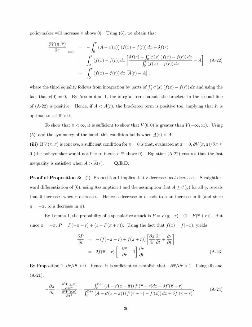
policymaker will increase π above 0). Using (6), we obtain that
∂V (π, π)
∂π
¯̄̄̄π=0
= −Z r
0
¡A− c0(x)
¢(f(x)− f(r))dx+ δf(r)
=
Z r
0(f(x)− f(r))dx
·δf(r) +
R r0 c
0(x) (f(x)− f(r)) dxR r0 (f(x)− f(r)) dx
−A
¸(A-22)
=
Z r
0(f(x)− f(r))dx
£A(r)−A
¤,
where the third equality follows from integration by parts ofR r0 c
0(x) (f(x)− f(r))dx and using the
fact that c(0) = 0. By Assumption 1, the integral term outside the brackets in the second line
of (A-22) is positive. Hence, if A < A(r), the bracketed term is positive too, implying that it is
optimal to set π > 0.
To show that π <∞, it is sufficient to show that V (0, 0) is greater than V (−∞,∞). Using(5), and the symmetry of the band, this condition holds when A(r) < A.
(iii) If V (π, π) is concave, a sufficient condition for π = 0 is that, evaluated at π = 0, ∂V (π, π)/∂π ≤0 (the policymaker would not like to increase π above 0). Equation (A-22) ensures that the last
inequality is satisfied when A > A(r). Q.E.D.
Proof of Proposition 3: (i) Proposition 1 implies that r decreases as t decreases. Straightfor-
ward differentiation of (6), using Assumption 1 and the assumption that A ≥ c0(y) for all y, reveals
that π̄ increases when r decreases. Hence a decrease in t leads to a an increase in π̄ (and since
π = −π̄, to a decrease in π).
By Lemma 1, the probability of a speculative attack is P = F (π− r)+(1−F (π+ r)). But
since π = −π̄, P = F (−π − r) + (1− F (π + r)). Using the fact that f(x) = f(−x), yields
∂P
∂t= − (f(−π − r) + f(π + r))
·∂π
∂r
∂r
∂t+
∂r
∂t
¸= 2f(π + r)
·−∂π∂r− 1¸∂r
∂t. (A-23)
By Proposition 1, ∂r/∂t > 0. Hence, it is sufficient to establish that −∂π/∂r > 1. Using (6) and(A-21),
−∂π∂r
=∂2V (π,π)∂π∂r
∂2V (π,π)∂π2
=
R π+rπ (A− c0(x− π)) f 0(π + r)dx+ δf 0(π + r)R π+r
π (A− c0(x− π)) (f 0(π + r)− f 0(x)) dx+ δf 0(π + r). (A-24)
36
The second-order condition for an internal solution for π implies that the denominator of this
expression is negative. Assumption 1 and A > c0(y) for all y imply that the numerator is negative
as well. But the denominator is equal to the numerator minusR π+rπ (A− c0(x− π)) f 0(x)dx.
Assumption 1 and A > c0(y) for all y imply that this expression is negative. It follows that
the denominator is smaller in absolute value than the numerator, implying that the expression in
equation (A-24) is larger than one.
(ii) Differentiating A(r) with respect to t yields:
∂A(r)
∂t=
(δ − c(r)) f 0(r)R r0 (f(x)− f(r))dx+
R r0 f
0(r)dx¡δf(r)− R r0 c(x)f 0(x)dx¢¡R r
0 (f(x)− f(r)) dx¢2 ∂r
∂t
= f 0(r)(δ − c(r))
R r0 f(x)dx+ rc(r)f(r)− r
R r0 c(x)f
0(x)dx¡R r0 (f(x)− f(r))dx
¢2 ∂r
∂t< 0, (A-25)
where the inequality follows because f 0(r) < 0 by Assumption 1, ∂r/∂t > 0 by Proposition 1, and
by (A-12), δ = C(r, α∗) > C(r, 0) ≡ c(r). Part (iii) of Proposition 2 implies that the policymaker
prefers to set a peg when A > A(r). Since A(r) falls with t, this condition is more likely to hold
when t is larger.
(iii) Using (5) for the case Eπ = 0 and the envelope theorem, it follows that:
∂V (π, π)
∂t= (rA− c(r) + δ) [f(π − r) + f(π + r)]
∂r
∂t> 0, (A-26)
where the inequality follows because δ > c(r) and because by Proposition 1, ∂r/∂t > 0. Q.E.D
Proof of Proposition 4: (i) The proof follows by straightforward differentiation of (6) with
respect to A and by using Assumption 1 and the fact that π = −π̄.(ii) By Lemma 1, the probability of a speculative attack is P = F (π− r) + (1−F (π+ r)).
Straightforward differentiation of P with respect to A, along with part (i) of the proposition,
establish the result. Q.E.D.
Proof of Proposition 5: Let π̄f be the solution to the policymaker’s maximization problem when
the density function is f(x) and let π̄g be the corresponding solution when the density function is
g(x). π̄g is defined by (6) with g(x) replacing f(x). Now, let’s evaluate ∂V (π, π)/∂π when the
37
density is g(x) at π̄f .
∂V (π, π)
∂π̄
¯̄̄̄π̄=π̄f
= −Z π̄f+r
π̄f
³A− c0(x− π̄f )
´³g(x)− g(πf + r)
´dx+ δg(πf + r)
= −Z π̄f+r
π̄f
³A− c0(x− πf )
´³g(x)− f(πf + r)
´dx+ δf(πf + r) (A-27)
> −Z π̄f+r
π̄f
³A− c0(x− πf )
´³f(x)− f(πf + r)
´dx+ δf(πf + r) = 0,
where the first equality follows since, by assumption, g(πf +r) = f(πf +r). The inequality follows
because f(x) lies above g(x) whenever x < πf + r, and the last equality follows from the first-order
condition in (6). Since (A-27) implies that ∂V (π, π)/∂π|π̄=π̄f > 0, it follows that π̄f < π̄g. The
analogous result for the lower bound of the band follows by recalling that, since the two distributions
and the corresponding optimal bands are symmetric, πg = −π̄g and πf = −π̄f . Q.E.D.
38
7 References
Angeletos, George M., Christian Hellwig and Alessandro Pavan (2002). “Coordination and Policy
Traps in Currency Crises.” Working paper, MIT.
Barro, Robert J. (1986). “Reputation in a Model of Monetary Policy with Incomplete
Information.” Journal of Monetary Economics, 17, pp. 3—20.
Barro, Robert J. and David B. Gordon (1983). “A Positive Theory of Monetary Policy in
a Natural Rate Model.” Journal of Political Economy, 91, pp. 589—610.
Bartolini, Leonardo and Alessandro Prati (1999). “Soft exchange-rate bands and Specula-
tive Attacks: Theory and Evidence from the ERM since August 1993.” Journal of International
Economics, 49, pp. 1—29.
Berglund, Tom, Seppo Honkapohja, Anne Mikkola, and Antti Suvanto (2001). “Promoting
the Stability of International Capital Movements.” Research Report 1/2001, Ministry of Finance,
Finland.
Bertola, Giuseppe and Ricardo J. Caballero (1992). “Target Zones and Realignments.”
American Economic Review, 82, pp. 520—536.
Bertola, Giuseppe and Lars O. Svensson (1993). “Stochastic Devaluations Risk and the
Empirical Fit of Target-Zone Models.” Review of Economic Studies, 60, pp. 689—712.
Calvo, Guillermo A. and Carmen M. Reinhart (2002). “Fear of Floating.” Quarterly Journal
of Economics, 117, pp. 379—408.
Carlsson, Hans and Eric van Damme (1993). “Global Games and Equilibrium Selection.”
Econometrica, 61, pp. 989—1018.
Chan, Kenneth and Stephen Chiu (2002). “The Role of (Non-) Transparency in a Currency
Crisis Model.” European Economic Review, 46, pp. 397—416.
Cukierman, Alex, Itay Goldstein, and Yossi Spiegel (2003). “The Choice of exchange-rate
regime and Speculative Attacks.” Working paper, Tel Aviv University. < http://www.tau.ac.il/
~alexcuk/pdf/bands3C33.pdf >.
Cukierman, Alex, Miguel Kiguel, and Nissan Liviatan (1992). “How Much to Commit to
an Exchange Rate Rule? Balancing Credibility and Flexibility.” Revista de Analisis Economico, 7,
39
pp. 73—90.
Cukierman, Alex, Yossi Spiegel, and Leonardo Leiderman (2004). “The Choice of exchange-
rate bands: Balancing Credibility and Flexibility.” Journal of International Economics, 62, pp.
379—408.
Cukierman, Alex and Paul Wachtel (1982). “Inflationary Expectations – Reply and Fur-
ther Thoughts on Inflation Uncertainty.” American Economic Review, 72, pp. 508—512.
Devereux, Michael and Charles Engel (1999). “Fixed vs. Floating Exchange Rates: How
Price Setting Affects Optimal Choice of Exchange-Rate Regime.” NBER Working Paper 6867.
Eichengreen, Barry (1999). Toward a New International Financial Architecture: A Practical
Post - Asia Agenda. Washington, DC: Institute for International Economics.
Eichengreen, Barry, James Tobin, and Charles Wyplosz (1995). “Two Cases for Sand in
the Wheels of International Finance.” Economic Journal, 105, pp. 162—172.
Fischer, Stanley (2001). “Distinguished Lecture on Economics in Government: exchange-
rate regimes: Is the Bipolar View Correct?” Journal of Economic Perspectives, 15, pp. 3—24.
Flood, Robert and Peter Garber (1984). “Collapsing exchange-rate regimes, Some Linear
Examples.” Journal of International Economics, 17, pp. 1—13.
Flood, Robert and Nancy Marion (1999). “Perspectives on the Recent Currency Crisis
Literature.” International Journal of Finance and Economics, 4, pp. 1—26.
Garber, Peter and Lars O. Svensson (1995). “The Operation and Collapse of Fixed exchange-
rate regimes.” In Handook of International Economics, vol. 3, edited by Gene Grossman and
Kenneth Rogoff. Elsevier.
Goldstein, Itay and Ady Pauzner (2004). “Demand Deposit Contracts and The Probability
of Bank Runs.” Journal of Finance, forthcoming.
Guembel, Alexander and Oren Sussman (2004). “Optimal Exchange Rates: A Market-
Microstructure Approach.” Journal of the European Economic Association, forthcoming.
Gylfason, Thorvaldur (2000). “Fix or Flex? Alternative exchange-rate regimes in an Era
of Global Capital Mobility.” North American Journal of Economics and Finance, 11, pp. 173—189.
Haq, Mahbubul, Inge Kaul, and Isabelle Grunberg (1996). The Tobin Tax: Coping with
40
Financial Volatility. Oxford University Press.
Heinemann, Frank and Gerhard Illing (2002). “Speculative Attacks: Unique Equilibrium
and Transparency.” Journal of International Economics, 58, pp. 429—450.
Helpman, Elhanan and Assaf Razin (1982). “A Comparison of exchange-rate regimes in
the Presence of Imperfect Capital Markets.” International Economic Review, 23, pp. 365—388.
Isard, Peter (1995). Exchange Rate Economics. Cambridge University Press.
Jeanne, Olivier (1996). “Would a Tobin Tax Have Saved the EMS?” Scandinavian Journal
of Economics, 98, pp. 503—520.
Jeanne, Olivier (2000). “Currency Crises: A Perspective on Recent Theoretical Develop-
ments.” Special Papers in International Economics, No. 20, International Finance Section, Prince-
ton University.
Jeanne, Olivier and Andrew K. Rose (2002). “Noise Trading and exchange-rate regimes.”
Quarterly Journal of Economics, 117, pp. 537—569.
Koren, Miklos (2000). “Implicit Band within the Announced exchange-rate band.” Rajk
Laszlo Szakkolegium WP no. 5.
Krugman, Paul (1979). “AModel of Balance-of-Payments Crises.” Journal of Money, Credit
and Banking, 11, pp. 311—325.
Krugman, Paul (1991). “Target Zones and Exchange Rate Dynamics.” Quarterly Journal
of Economics, 106, pp. 669—682.
Kupiec, Paul H. (1996). “Noise Traders, Excess Volatility, and a Securities Transactions
Tax.” Journal of Financial Services Research, 10, pp. 115—129.
Kydland, Finn and Edward C. Prescott (1977). “Rules Rather than Discretion: The Incon-
sistency of Optimal Plans.” Journal of Political Economy, 85, pp. 473—492.
Lohmann, Susanne (1992). “Optimal Commitment in Monetary Policy: Credibility versus
Flexibility.” American Economic Review, 82, pp. 273—286.
McKinnon, Ronald (1979). Money in International Exchange – The Convertible Currency
System. Oxford University Press.
McKinnon, Ronald (2000). “On the Pheriphery of the International Dollar Standard:
41
Canada, Latin America, and East Asia.” North American Journal of Economics and Finance,
11, pp. 105—121.
McKinnon, Ronald (2001). “After the Crisis, the East Asian Dollar Standard Resurrected:
An Interpretation of High Frequency Exchange Rate Pegging.” In Rethinking the East Asia Miracle,
edited by Joseph E. Stiglitz and Shahid Yusuf. Oxford University Press and World Bank.
Miller, Marcus and Lei Zhang (1996). “Optimal Target Zones: How an Exchange Rate
Mechanism Can Improve Upon Discretion?” Journal of Economic Dynamics and Control, 20, pp.
1641—1660.
Morris, Stephen and Hyun S. Shin (1998). “Unique Equilibrium in a Model of Self-Fulfilling
Currency Attacks.” American Economic Review, 88, pp. 587—597.
Morris, Stephen and Hyun S. Shin (2003). “Global Games: Theory and Applications.”
In Advances in Economics and Econometrics, edited by Mathias Dewatripont, Lars Hansen, and
Stephen Turnovsky. Cambridge University Press.
Obstfeld, Maurice (1994). “The Logic of Currency Crises.” Cahiers Economiques et Mon-
etaires, 43, pp. 189—213.
Obstfeld, Maurice (1996). “Models of Currency Crises with Self-Fulfilling Features.” Euro-
pean Economic Review, 40, pp. 1037—1047.
Obstfeld, Maurice (1997). “Destabilizing Effects of Exchange-Rate Escape Clauses.” Jour-
nal of International Economics, 43, pp. 61—77.
Sutherland, Alan (1995). “Monetary and Real Shocks and the Optimal Target Zone.”
European Economic Review, 39, pp. 161—172.
Tobin, James (1978). “A Proposal for International Monetary Reform.” Eastern Economic
Journal, 153, pp. 1—15.
Velasco, Andres (1997). “When are Fixed Exchange Rates Really Fixed?” Journal of De-
velopment Economics, 54, pp. 5—25.
Wagner, Helmut (2000). “Which exchange-rate regimes in an Era of High Capital Mobil-
ity?” North American Journal of Economics and Finance, 11, pp. 191—203.
42