The Chicago Plan Revisited

Jaromir Benes and Michael Kumhof

WP/12/202

© 2012 International Monetary Fund WP/12/202

IMF Working Paper

Research Department

The Chicago Plan Revisited

Prepared by Jaromir Benes and Michael Kumhof

Authorized for distribution by Douglas Laxton

August 2012

This Working Paper should not be reported as representing the views of the IMF.

The views expressed in this Working Paper are those of the author(s) and do not necessarily represent

those of the IMF or IMF policy. Working Papers describe research in progress by the author(s) and are

published to elicit comments and to further debate.

Abstract

At the height of the Great Depression a number of leading U.S. economists advanced a

proposal for monetary reform that became known as the Chicago Plan. It envisaged the

separation of the monetary and credit functions of the banking system, by requiring 100%

reserve backing for deposits. Irving Fisher (1936) claimed the following advantages for this

plan: (1) Much better control of a major source of business cycle fluctuations, sudden

increases and contractions of bank credit and of the supply of bank-created money.

(2) Complete elimination of bank runs. (3) Dramatic reduction of the (net) public debt.

(4) Dramatic reduction of private debt, as money creation no longer requires simultaneous

debt creation. We study these claims by embedding a comprehensive and carefully calibrated

model of the banking system in a DSGE model of the U.S. economy. We find support for all

four of Fisher's claims. Furthermore, output gains approach 10 percent, and steady state

inflation can drop to zero without posing problems for the conduct of monetary policy.

JEL Classification Numbers: E44, E52, G21

Keywords: Chicago Plan; Chicago School of Economics; 100% reserve banking; bank

lending; lending risk; private money creation; bank capital adequacy;

government debt; private debt; boom-bust cycles.

Authors’ E-Mail Addresses: jbenes@imf.org; mkumhof@imf.org

2

Contents

I. Introduction . . . . . . . . . . . . . . . . . . . . . . . . . . . . . . . . . . . . . 4

II. The Chicago Plan in the History of Monetary Thought . . . . . . . . . . . . . 12A. Government versus Private Control over Money Issuance . . . . . . . . . 12B. The Chicago Plan . . . . . . . . . . . . . . . . . . . . . . . . . . . . . . . 17

III. The Model under the Current Monetary System . . . . . . . . . . . . . . . . . 20A. Banks . . . . . . . . . . . . . . . . . . . . . . . . . . . . . . . . . . . . . . 20B. Lending Technologies . . . . . . . . . . . . . . . . . . . . . . . . . . . . . 24C. Transactions Cost Technologies . . . . . . . . . . . . . . . . . . . . . . . 26D. Equity Ownership and Dividends . . . . . . . . . . . . . . . . . . . . . . 26E. Unconstrained Households . . . . . . . . . . . . . . . . . . . . . . . . . . 27F. Constrained Households . . . . . . . . . . . . . . . . . . . . . . . . . . . . 28G. Unions . . . . . . . . . . . . . . . . . . . . . . . . . . . . . . . . . . . . . 30H. Manufacturers . . . . . . . . . . . . . . . . . . . . . . . . . . . . . . . . . 30I. Capital Goods Producers . . . . . . . . . . . . . . . . . . . . . . . . . . . 31J. Capital Investment Funds . . . . . . . . . . . . . . . . . . . . . . . . . . . 31K. Government . . . . . . . . . . . . . . . . . . . . . . . . . . . . . . . . . . 32

1. Monetary Policy . . . . . . . . . . . . . . . . . . . . . . . . . . . . . 322. Prudential Policy . . . . . . . . . . . . . . . . . . . . . . . . . . . . 323. Fiscal Policy . . . . . . . . . . . . . . . . . . . . . . . . . . . . . . . 324. Government Budget Constraint . . . . . . . . . . . . . . . . . . . . 33

L. Market Clearing . . . . . . . . . . . . . . . . . . . . . . . . . . . . . . . . 33

IV. The Model under the Chicago Plan . . . . . . . . . . . . . . . . . . . . . . . . 33A. Banks . . . . . . . . . . . . . . . . . . . . . . . . . . . . . . . . . . . . . . 33B. Households . . . . . . . . . . . . . . . . . . . . . . . . . . . . . . . . . . . 36C. Manufacturers . . . . . . . . . . . . . . . . . . . . . . . . . . . . . . . . . 37D. Government . . . . . . . . . . . . . . . . . . . . . . . . . . . . . . . . . . 37

1. Monetary Policy . . . . . . . . . . . . . . . . . . . . . . . . . . . . . 372. Prudential Policy . . . . . . . . . . . . . . . . . . . . . . . . . . . . 393. Fiscal Policy . . . . . . . . . . . . . . . . . . . . . . . . . . . . . . . 404. Government Budget Constraint . . . . . . . . . . . . . . . . . . . . 415. Controlling Boom-Bust Cycles - Additional Considerations . . . . . 42

V. Calibration . . . . . . . . . . . . . . . . . . . . . . . . . . . . . . . . . . . . . . 42

VI. Transition to the Chicago Plan . . . . . . . . . . . . . . . . . . . . . . . . . . . 49

VII. Credit Booms and Busts Pre-Transition and Post-Transition . . . . . . . . . . 52

VIII. Conclusion . . . . . . . . . . . . . . . . . . . . . . . . . . . . . . . . . . . . . . 55

References . . . . . . . . . . . . . . . . . . . . . . . . . . . . . . . . . . . . . . . . . . 57

3

Figures

1. Changes in Bank Balance Sheet in Transition Period (percent of GDP) . . . . 642. Changes in Government Balance Sheet in Transition Period (percent of GDP) 653. Changes in Bank Balance Sheet - Details (percent of GDP) . . . . . . . . . . 664. Transition to Chicago Plan - Bank Balance Sheets . . . . . . . . . . . . . . . . 675. Transition to Chicago Plan - Main Macroeconomic Variables . . . . . . . . . . 686. Transition to Chicago Plan - Fiscal Variables . . . . . . . . . . . . . . . . . . 697. Business Cycle Properties Pre-Transition versus Post-Transition . . . . . . . . 70

4

I. Introduction

The decade following the onset of the Great Depression was a time of great intellectualferment in economics, as the leading thinkers of the time tried to understand the apparentfailures of the existing economic system. This intellectual struggle extended to manydomains, but arguably the most important was the field of monetary economics, given thekey roles of private bank behavior and of central bank policies in triggering andprolonging the crisis.

During this time a large number of leading U.S. macroeconomists supported afundamental proposal for monetary reform that later became known as the Chicago Plan,after its strongest proponent, professor Henry Simons of the University of Chicago. It wasalso supported, and brilliantly summarized, by Irving Fisher of Yale University, in Fisher(1936). The key feature of this plan was that it called for the separation of the monetaryand credit functions of the banking system, first by requiring 100% backing of deposits bygovernment-issued money, and second by ensuring that the financing of new bank creditcan only take place through earnings that have been retained in the form ofgovernment-issued money, or through the borrowing of existing government-issued moneyfrom non-banks, but not through the creation of new deposits, ex nihilo, by banks.

Fisher (1936) claimed four major advantages for this plan. First, preventing banks fromcreating their own funds during credit booms, and then destroying these funds duringsubsequent contractions, would allow for a much better control of credit cycles, whichwere perceived to be the major source of business cycle fluctuations. Second, 100% reservebacking would completely eliminate bank runs. Third, allowing the government to issuemoney directly at zero interest, rather than borrowing that same money from banks atinterest, would lead to a reduction in the interest burden on government finances and to adramatic reduction of (net) government debt, given that irredeemable government-issuedmoney represents equity in the commonwealth rather than debt. Fourth, given thatmoney creation would no longer require the simultaneous creation of mostly private debtson bank balance sheets, the economy could see a dramatic reduction not only ofgovernment debt but also of private debt levels.

We take it as self-evident that if these claims can be verified, the Chicago Plan wouldindeed represent a highly desirable policy. Profound thinkers like Fisher, and many of hismost illustrious peers, based their insights on historical experience and common sense, andwere hardly deterred by the fact that they might not have had complete economic modelsthat could formally derive the welfare gains of avoiding credit-driven boom-bust cycles,bank runs, and high debt levels. We do in fact believe that this made them better, notworse, thinkers about issues of the greatest importance for the common good. But we cansay more than this. The recent empirical evidence of Reinhart and Rogoff (2009)documents the high costs of boom-bust credit cycles and bank runs throughout history.And the recent empirical evidence of Schularick and Taylor (2012) is supportive of Fisher’sview that high debt levels are a very important predictor of major crises. The latterfinding is also consistent with the theoretical work of Kumhof and Rancière (2010), whoshow how very high debt levels, such as those observed just prior to the Great Depressionand the Great Recession, can lead to a higher probability of financial and real crises.

5

We now turn to a more detailed discussion of each of Fisher’s four claims concerning theadvantages of the Chicago Plan. This will set the stage for a first illustration of theimplied balance sheet changes, which will be provided in Figures 1 and 2.

The first advantage of the Chicago Plan is that it permits much better control of whatFisher and many of his contemporaries perceived to be the major source of business cyclefluctuations, sudden increases and contractions of bank credit that are not necessarilydriven by the fundamentals of the real economy, but that themselves change thosefundamentals. In a financial system with little or no reserve backing for deposits, and withgovernment-issued cash having a very small role relative to bank deposits, the creation ofa nation’s broad monetary aggregates depends almost entirely on banks’ willingness tosupply deposits. Because additional bank deposits can only be created through additionalbank loans, sudden changes in the willingness of banks to extend credit must therefore notonly lead to credit booms or busts, but also to an instant excess or shortage of money, andtherefore of nominal aggregate demand. By contrast, under the Chicago Plan the quantityof money and the quantity of credit would become completely independent of each other.This would enable policy to control these two aggregates independently and thereforemore effectively. Money growth could be controlled directly via a money growth rule. Thecontrol of credit growth would become much more straightforward because banks wouldno longer be able, as they are today, to generate their own funding, deposits, in the act oflending, an extraordinary privilege that is not enjoyed by any other type of business.Rather, banks would become what many erroneously believe them to be today, pureintermediaries that depend on obtaining outside funding before being able to lend. Havingto obtain outside funding rather than being able to create it themselves would muchreduce the ability of banks to cause business cycles due to potentially capricious changesin their attitude towards credit risk.

The second advantage of the Chicago Plan is that having fully reserve-backed bankdeposits would completely eliminate bank runs, thereby increasing financial stability, andallowing banks to concentrate on their core lending function without worrying aboutinstabilities originating on the liabilities side of their balance sheet. The elimination ofbank runs will be accomplished if two conditions hold. First, the banking system’smonetary liabilities must be fully backed by reserves of government-issued money, which isof course true under the Chicago Plan. Second, the banking system’s credit assets must befunded by non-monetary liabilities that are not subject to runs. This means that policyneeds to ensure that such liabilities cannot become near-monies. The literature of the1930s and 1940s discussed three institutional arrangements under which this can beaccomplished. The easiest is to require that banks fund all of their credit assets with acombination of equity and loans from the government treasury, and completely withoutprivate debt instruments. This is the core element of the version of the Chicago Planconsidered in this paper, because it has a number of advantages that go beyond decisivelypreventing the emergence of near-monies. By itself this would mean that there is nolending at all between private agents. However, this can be insufficient when private agentsexhibit highly heterogeneous initial debt levels. In that case the treasury loans solutioncan be accompanied by either one or both of the other two institutional arrangements.One is debt-based investment trusts that are true intermediaries, in that the trust canonly lend government-issued money to net borrowers after net savers have first depositedthese funds in exchange for debt instruments issued by the trust. But there is a risk that

6

these debt instruments could themselves become near-monies unless there are strict andeffective regulations. This risk would be eliminated under the remaining alternative,investment trusts that are funded exclusively by net savers’ equity investments, with thefunds either lent to net borrowers, or invested as equity if this is feasible (it may not befeasible for household debtors). We will briefly return to the investment trust alternativesbelow, but they are not part of our formal analysis because our model does not featureheterogeneous debt levels within the four main groups of bank borrowers.

The third advantage of the Chicago Plan is a dramatic reduction of (net) governmentdebt. The overall outstanding liabilities of today’s U.S. financial system, including theshadow banking system, are far larger than currently outstanding U.S. Treasury liabilities.Because under the Chicago Plan banks have to borrow reserves from the treasury to fullyback these large liabilities, the government acquires a very large asset vis-à-vis banks, andgovernment debt net of this asset becomes highly negative. Governments could leave theseparate gross positions outstanding, or they could buy back government bonds frombanks against the cancellation of treasury credit. Fisher had the second option in mind,based on the situation of the 1930s, when banks held the major portion of outstandinggovernment debt. But today most U.S. government debt is held outside U.S. banks, sothat the first option is the more relevant one. The effect on net debt is of course the same,it drops dramatically.

In this context it is critical to realize that the stock of reserves, or money, newly issued bythe government is not a debt of the government. The reason is that fiat money is notredeemable, in that holders of money cannot claim repayment in something other thanmoney.1 Money is therefore properly treated as government equity rather thangovernment debt, which is exactly how treasury coin is currently treated under U.S.accounting conventions (Federal Accounting Standards Advisory Board (2012)).

The fourth advantage of the Chicago Plan is the potential for a dramatic reduction ofprivate debts. As mentioned above, full reserve backing by itself would generate a highlynegative net government debt position. Instead of leaving this in place and becoming alarge net lender to the private sector, the government has the option of spending part ofthe windfall by buying back large amounts of private debt from banks against thecancellation of treasury credit. Because this would have the advantage of establishinglow-debt sustainable balance sheets in both the private sector and the government, it isplausible to assume that a real-world implementation of the Chicago Plan would involveat least some, and potentially a very large, buy-back of private debt. In the simulation ofthe Chicago Plan presented in this paper we will assume that the buy-back covers allprivate bank debt except loans that finance investment in physical capital.

We study Fisher’s four claims by embedding a comprehensive and carefully calibratedmodel of the U.S. financial system in a state-of-the-art monetary DSGE model of the U.S.economy.2 We find strong support for all four of Fisher’s claims, with the potential formuch smoother business cycles, no possibility of bank runs, a large reduction of debt levelsacross the economy, and a replacement of that debt by debt-free government-issued money.

1Furthermore, in a growing economy the government will never have a need to voluntarily retire moneyto maintain price stability, as the economy’s monetary needs increase period after period.

2To our knowledge this is the first attempt to model the Chicago Plan in this way. Yamaguchi (2011)discusses the Chicago Plan using a systems dynamics approach.

7

Furthermore, none of these benefits come at the expense of diminishing the core usefulfunctions of a private financial system. Under the Chicago Plan private financialinstitutions would continue to play a key role in providing a state-of-the-art paymentssystem, facilitating the efficient allocation of capital to its most productive uses, andfacilitating intertemporal smoothing by households and firms. Credit, especially sociallyuseful credit that supports real physical investment activity, would continue to exist.What would cease to exist however is the proliferation of credit created, at the almostexclusive initiative of private institutions, for the sole purpose of creating an adequatemoney supply that can easily be created debt-free.

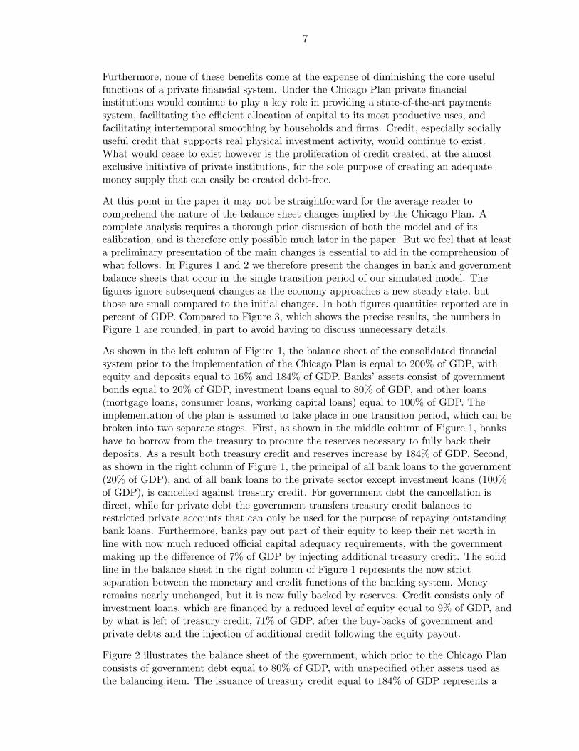
At this point in the paper it may not be straightforward for the average reader tocomprehend the nature of the balance sheet changes implied by the Chicago Plan. Acomplete analysis requires a thorough prior discussion of both the model and of itscalibration, and is therefore only possible much later in the paper. But we feel that at leasta preliminary presentation of the main changes is essential to aid in the comprehension ofwhat follows. In Figures 1 and 2 we therefore present the changes in bank and governmentbalance sheets that occur in the single transition period of our simulated model. Thefigures ignore subsequent changes as the economy approaches a new steady state, butthose are small compared to the initial changes. In both figures quantities reported are inpercent of GDP. Compared to Figure 3, which shows the precise results, the numbers inFigure 1 are rounded, in part to avoid having to discuss unnecessary details.

As shown in the left column of Figure 1, the balance sheet of the consolidated financialsystem prior to the implementation of the Chicago Plan is equal to 200% of GDP, withequity and deposits equal to 16% and 184% of GDP. Banks’ assets consist of governmentbonds equal to 20% of GDP, investment loans equal to 80% of GDP, and other loans(mortgage loans, consumer loans, working capital loans) equal to 100% of GDP. Theimplementation of the plan is assumed to take place in one transition period, which can bebroken into two separate stages. First, as shown in the middle column of Figure 1, bankshave to borrow from the treasury to procure the reserves necessary to fully back theirdeposits. As a result both treasury credit and reserves increase by 184% of GDP. Second,as shown in the right column of Figure 1, the principal of all bank loans to the government(20% of GDP), and of all bank loans to the private sector except investment loans (100%of GDP), is cancelled against treasury credit. For government debt the cancellation isdirect, while for private debt the government transfers treasury credit balances torestricted private accounts that can only be used for the purpose of repaying outstandingbank loans. Furthermore, banks pay out part of their equity to keep their net worth inline with now much reduced official capital adequacy requirements, with the governmentmaking up the difference of 7% of GDP by injecting additional treasury credit. The solidline in the balance sheet in the right column of Figure 1 represents the now strictseparation between the monetary and credit functions of the banking system. Moneyremains nearly unchanged, but it is now fully backed by reserves. Credit consists only ofinvestment loans, which are financed by a reduced level of equity equal to 9% of GDP, andby what is left of treasury credit, 71% of GDP, after the buy-backs of government andprivate debts and the injection of additional credit following the equity payout.

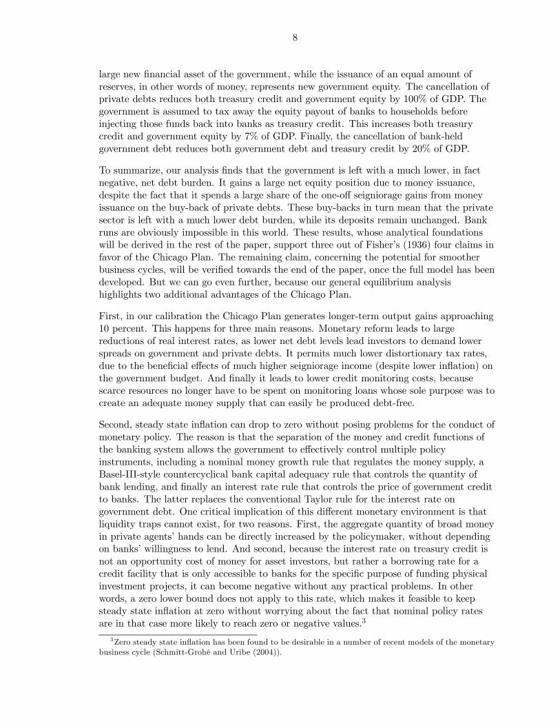
Figure 2 illustrates the balance sheet of the government, which prior to the Chicago Planconsists of government debt equal to 80% of GDP, with unspecified other assets used asthe balancing item. The issuance of treasury credit equal to 184% of GDP represents a

8

large new financial asset of the government, while the issuance of an equal amount ofreserves, in other words of money, represents new government equity. The cancellation ofprivate debts reduces both treasury credit and government equity by 100% of GDP. Thegovernment is assumed to tax away the equity payout of banks to households beforeinjecting those funds back into banks as treasury credit. This increases both treasurycredit and government equity by 7% of GDP. Finally, the cancellation of bank-heldgovernment debt reduces both government debt and treasury credit by 20% of GDP.

To summarize, our analysis finds that the government is left with a much lower, in factnegative, net debt burden. It gains a large net equity position due to money issuance,despite the fact that it spends a large share of the one-off seigniorage gains from moneyissuance on the buy-back of private debts. These buy-backs in turn mean that the privatesector is left with a much lower debt burden, while its deposits remain unchanged. Bankruns are obviously impossible in this world. These results, whose analytical foundationswill be derived in the rest of the paper, support three out of Fisher’s (1936) four claims infavor of the Chicago Plan. The remaining claim, concerning the potential for smootherbusiness cycles, will be verified towards the end of the paper, once the full model has beendeveloped. But we can go even further, because our general equilibrium analysishighlights two additional advantages of the Chicago Plan.

First, in our calibration the Chicago Plan generates longer-term output gains approaching10 percent. This happens for three main reasons. Monetary reform leads to largereductions of real interest rates, as lower net debt levels lead investors to demand lowerspreads on government and private debts. It permits much lower distortionary tax rates,due to the beneficial effects of much higher seigniorage income (despite lower inflation) onthe government budget. And finally it leads to lower credit monitoring costs, becausescarce resources no longer have to be spent on monitoring loans whose sole purpose was tocreate an adequate money supply that can easily be produced debt-free.

Second, steady state inflation can drop to zero without posing problems for the conduct ofmonetary policy. The reason is that the separation of the money and credit functions ofthe banking system allows the government to effectively control multiple policyinstruments, including a nominal money growth rule that regulates the money supply, aBasel-III-style countercyclical bank capital adequacy rule that controls the quantity ofbank lending, and finally an interest rate rule that controls the price of government creditto banks. The latter replaces the conventional Taylor rule for the interest rate ongovernment debt. One critical implication of this different monetary environment is thatliquidity traps cannot exist, for two reasons. First, the aggregate quantity of broad moneyin private agents’ hands can be directly increased by the policymaker, without dependingon banks’ willingness to lend. And second, because the interest rate on treasury credit isnot an opportunity cost of money for asset investors, but rather a borrowing rate for acredit facility that is only accessible to banks for the specific purpose of funding physicalinvestment projects, it can become negative without any practical problems. In otherwords, a zero lower bound does not apply to this rate, which makes it feasible to keepsteady state inflation at zero without worrying about the fact that nominal policy ratesare in that case more likely to reach zero or negative values.3

3Zero steady state inflation has been found to be desirable in a number of recent models of the monetarybusiness cycle (Schmitt-Grohé and Uribe (2004)).

9

The ability to live with significantly lower steady state inflation also answers thesomewhat confused claim of opponents of an exclusive government monopoly on moneyissuance, namely that such a system, and especially the initial injection of newgovernment-issued money, would be highly inflationary. There is nothing in our theorythat supports this claim. And as we will see in section II, there is also virtually nothing inthe monetary history of ancient societies and of Western nations that supports this claim.

The critical feature of our theoretical model is that it exhibits the key function of banks inmodern economies, which is not their largely incidental function as financial intermediariesbetween depositors and borrowers, but rather their central function as creators anddestroyers of money.4 A realistic model needs to reflect the fact that under the presentsystem banks do not have to wait for depositors to appear and make funds availablebefore they can on-lend, or intermediate, those funds. Rather, they create their ownfunds, deposits, in the act of lending. This fact can be verified in the description of themoney creation system in many central bank statements5, and it is obvious to anybodywho has ever lent money and created the resulting book entries.6 In other words, bankliabilities are not macroeconomic savings, even though at the microeconomic level theycan appear as such. Savings are a state variable, so that by relying entirely onintermediating slow-moving savings, banks would be unable to engineer the rapid lendingbooms and busts that are frequently observed in practice. Rather, bank liabilities aremoney that can be created and destroyed at a moment’s notice. The critical importance ofthis fact appears to have been lost in much of the modern macroeconomics literature onbanking, with the exception of Werner (2005), and the partial exception of Christiano etal. (2011).7 Our model generates this feature in a number of ways. First, it introducesagents who have to borrow for the sole purpose of generating sufficient deposits for theirtransactions purposes. This means that they simultaneously borrow from and depositwith banks, as is true for many households and firms in the real world. Second, the modelintroduces financially unconstrained agents who do not borrow from banks. Their savingsconsist of multiple assets including a fixed asset referred to as land, government bonds anddeposits. This means that a sale of mortgageable fixed assets from these agents tocredit-constrained agents (or of government bonds to banks) results in new bank credit,and thus in the creation of new deposits that are created for the purpose of paying for

4The relative importance of these two features can be illustrated with a very simple thought experiment:Assume an economy with banks and a single homogenous group of non-bank private agents that has atransactions demand for money. In this economy there is no intermediation whatsoever, yet banks remaincritical. Their function is to create the money supply through the mortgaging of private agents’ assets. Wehave verified that such a model economy works very similarly to the one presented in this paper, whichfeatures several distinct groups of non-bank private agents.

5Berry et al. (2007), which was written by a team from the Monetary Analysis Division of the Bank ofEngland, states: “When banks make loans, they create additional deposits for those that have borrowed themoney.” Keister and McAndrews (2009), staff economists at the Federal Reserve Bank of New York, write:“Suppose that Bank A gives a new loan of $20 to Firm X, which continues to hold a deposit account withBank A. Bank A does this by crediting Firm X’s account by $20. The bank now has a new asset (the loanto Firm X) and an offsetting liability (the increase in Firm X’s deposit at the bank). Importantly, Bank Astill has [unchanged] reserves in its account. In other words, the loan to Firm X does not decrease Bank A’sreserve holdings at all.” Putting this differently, the bank does not lend out reserves (money) that it alreadyowns, rather it creates new deposit money ex nihilo.

6This includes one of the authors of this paper.7We emphasize that this exception is partial, because while bank deposits in Christiano et al. (2011) are

modelled as money, they are also, with the empirically insignificant exception of a possible substitution intocash, modelled as representing household savings. The latter is not true in our model.

10

those assets. Third, even for conventional deposit-financed investment loans thetransmission is from lending to savings and not the reverse. When banks decide to lendmore for investment purposes, say due to increased optimism about business conditions,they create additional purchasing power for investors by crediting their accounts, and it isthis purchasing power that makes the actual investment, and thus saving8, possible.Finally, the issue can be further illuminated by looking at it from the vantage point ofdepositors. We will assume, based on empirical evidence, that the interest rate sensitivityof deposit demand is high at the margin. Therefore, if depositors decided, for a givendeposit interest rate, that they wanted to start depositing additional funds in banks,without bankers wanting to make additional loans, the end result would be virtuallyunchanged deposits and loans. The reason is that banks would start to pay a slightlylower deposit interest rate, and this would be sufficient to strongly reduce deposit demandwithout materially affecting funding costs and therefore the volume of lending. The finaldecision on the quantity of deposit money in the economy is therefore almost exclusivelymade by banks, and is based on their optimism about business conditions.

Our model completely omits two other monetary magnitudes, cash outside banks andbank reserves held at the central bank. This is because it is privately created depositmoney that plays the central role in the current U.S. monetary system, whilegovernment-issued money plays a quantitatively and conceptually negligible role. Itshould be mentioned that both private and government-issued monies are fiat monies,because the acceptability of bank deposits for commercial and official transactions has hadto first be decreed by law. As we will argue in section II, virtually all monies throughouthistory, including precious metals, have derived most or all of their value from governmentfiat rather than from their intrinsic value.

Rogoff (1998) examines U.S. dollar currency outside banks for the late 1990s. Heconcludes that it was equal to around 5% of GDP for the United States, but that 95% ofthis was held either by foreigners and/or by the underground economy. This means thatcurrency outside banks circulating in the formal U.S. economy equalled only around 0.25%of GDP, while we will find that the current transactions-related liabilities of the U.S.financial system, including the shadow banking system, are equal to around 200% of GDP.

Bank reserves held at the central bank have also generally been negligible in size, exceptof course after the onset of the 2008 financial crisis. But this quantitative point is far lessimportant than the recognition that they do not play any meaningful role in thedetermination of wider monetary aggregates. The reason is that the “deposit multiplier”of the undergraduate economics textbook, where monetary aggregates are created at theinitiative of the central bank, through an initial injection of high-powered money into thebanking system that gets multiplied through bank lending, turns the actual operation ofthe monetary transmission mechanism on its head. This should be absolutely clear underthe current inflation targeting regime, where the central bank controls an interest rate andmust be willing to supply as many reserves as banks demand at that rate. But as shownby Kydland and Prescott (1990), the availability of central bank reserves did not evenconstrain banks during the period, in the 1970s and 1980s, when the central bank did infact officially target monetary aggregates.9 These authors show that broad monetary

8 In a closed economy saving must equal investment.9Carpenter and Demiralp (2010), in a Federal Reserve Board working paper, have found the same result,

11

aggregates, which are driven by banks’ lending decisions, led the economic cycle, whilenarrow monetary aggregates, most importantly reserves, lagged the cycle. In other words,at all times, when banks ask for reserves, the central bank obliges. Reserves thereforeimpose no constraint. The deposit multiplier is simply, in the words of Kydland andPrescott (1990), a myth.10 And because of this, private banks are almost fully in controlof the money creation process.

Apart from the central role of endogenous money, other features of our banking model arebased on Benes and Kumhof (2011). This work differs from other recent papers onbanking along several important dimensions. First, banks have their own balance sheetand net worth, and their profits and net worth are exposed to non-diversifiable aggregaterisk determined endogenously on the basis of optimal debt contracts.11 Second, banks arelenders rather than holders of risky equity.12 Third, bank lending is based on the loancontract of Bernanke, Gertler and Gilchrist (1999), but with the crucial difference thatlending is risky due to non-contingent lending interest rates. This implies that banks canmake losses if a larger number of loans defaults than was expected at the time of settingthe lending rate. Fourth, bank capital is subject to regulation that closely replicates thefeatures of the Basel regulatory framework, including costs of violating minimum capitaladequacy regulations. Capital buffers arise as an optimal equilibrium phenomenonresulting from the interaction of optimal debt contracts, endogenous losses andregulation.13 To maintain capital buffers, banks respond to loan losses by raising theirlending rate in order to rebuild their net worth, with adverse effects for the real economy.Fifth, acquiring fresh capital is subject to market imperfections. This is a necessarycondition for capital adequacy regulation to have non-trivial effects, and for the capitalbuffers to exist. We use the “extended family” approach of Gertler and Karadi (2010),whereby bankers (and also non-financial manufacturers and entrepreneurs) transfer part oftheir accumulated equity positions to the household budget constraint at an exogenouslyfixed rate. This is closely related to the original approach of Bernanke, Gertler andGilchrist (1999), and to the dividend policy function of Aoki, Proudman and Vlieghe(2004).

The rest of the paper is organized as follows. Section II contains a survey of the literatureon monetary history and monetary thought leading up to the Chicago Plan. Section IIIpresents an outline of the model under the current monetary system. Section IV presentsthe model under the Chicago Plan. Section V discusses model calibration. Section VIstudies impulse responses that simulate a dynamic transition between the currentmonetary system and the Chicago Plan, which allows us to analyze three of the fourabove-mentioned claims in favor of the Chicago Plan made by Fisher (1936). Theremaining claim, regarding the more effective stabilization of bank-driven business cycles,is studied in Section VII. Section VIII concludes.

using more recent data and a different methodology.10This is of course the reason why quantitative easing, at least the kind that works by making greater

reserves available to banks and not the public, can be ineffective if banks decide that lending remains toorisky.

11Christiano, Motto and Rostagno (2010) and Curdia and Woodford (2010) focus exclusively on how theprice of credit affects real activity.

12Gertler and Karadi (2010) and Angeloni and Faia (2009) make the latter assumption.13Van den Heuvel (2008) models capital adequacy as a continously binding constraint. Gerali et al. (2010)

use a quadratic cost short-cut.

12

II. The Chicago Plan in the History of Monetary Thought

A. Government versus Private Control over Money Issuance

The monetary historian Alexander Del Mar (1895) writes: “As a rule political economistsdo not take the trouble to study the history of money; it is much easier to imagine it andto deduce the principles of this imaginary knowledge.” Del Mar wrote more than a centuryago, but this statement still applies today. An excellent example is the textbookexplanation for the origins of money, which holds that money arose in private tradingtransactions, to overcome the double coincidence of wants problem of barter.14 As shownby Graeber (2011), on the basis of extensive anthropological and historical evidence thatgoes back millennia, there is not a shred of evidence to support this story. Barter wasvirtually nonexistent in primitive and ancient societies, and instead the first commercialtransactions took place on the basis of elaborate credit systems whose denomination wastypically in agricultural commodities, including cattle, grain by weight, and tools.Furthermore, Graeber (2011), Zarlenga (2002) and the references cited therein provideplenty of evidence that these credit systems, and the much later money systems, had theirorigins in the needs of the state (Ridgeway (1892)), of religious/temple institutions (Einzig(1966), Laum (1924)) and of social ceremony (Quiggin (1949)), and not in the needs ofprivate trading relationships.

Any debate on the origins of money is not of merely academic interest, because it leadsdirectly to a debate on the nature of money, which in turn has a critical bearing onarguments as to who should control the issuance of money. Specifically, the privatetrading story for the origins of money has time and again, starting at least with AdamSmith (1776), been used as an argument for the private issuance and control of money.Until recent times this has mainly taken the form of monetary systems based on preciousmetals, especially under free coinage of bullion into coins. Even though there can at timesbe heavy government involvement in such systems, the fact is that in practice preciousmetals tended to accumulate privately in the hands of the wealthy, who would then lendthem out at interest. Since the thirteenth century this precious-metals-based system has,in Europe, been accompanied, and increasingly supplanted, by the private issuance ofbank money, more properly called credit. On the other hand, the historically andanthropologically correct state/institutional story for the origins of money is one of thearguments supporting the government issuance and control of money under the rule oflaw. In practice this has mainly taken the form of interest-free issuance of notes or coins,although it could equally take the form of electronic deposits.

There is another issue that tends to get confused with the much more fundamental debateconcerning the control over the issuance of money, namely the debate over “real”precious-metals-backed money versus fiat money. As documented in Zarlenga (2002), thisdebate is mostly a diversion, because even during historical regimes based on preciousmetals the main reason for the high relative value of precious metals was precisely theirrole as money, which derives from government fiat and not from the intrinsic qualities ofthe metals.15 These matters are especially confused in Smith (1776), who takes a

14A typical early example of this claim is found in Menger (1892).15For example, in many of the ancient Greek societies gold was not intrinsically valuable due to scarcity,

13

primitive commodity view of money despite the fact that at his time the then privateBank of England had long since started to issue a fiat currency whose value wasessentially unrelated to the production cost of precious metals. Furthermore, as Smithcertainly knew, both the Bank of England and private banks were creating checkable bookcredits in accounts for borrowing customers who had not made any deposits of coin (oreven of bank notes).

The historical debate concerning the nature and control of money is the subject ofZarlenga (2002), a masterful work that traces this debate back to ancient Mesopotamia,Greece and Rome. Like Graeber (2011), he shows that private issuance of money hasrepeatedly led to major societal problems throughout recorded history, due to usuryassociated with private debts.16 Zarlenga does not adopt the common but simplisticdefinition of usury as the charging of “excessive interest”, but rather as “taking somethingfor nothing” through the calculated misuse of a nation’s money system for private gain.Historically this has taken two forms. The first form of usury is the private appropriationof the convenience yield of a society’s money. Private money has to be borrowed intoexistence at a positive interest rate, while the holders of that money, due to thenon-pecuniary benefits of its liquidity, are content to receive no or very low interest.Therefore, while part of the interest difference between lending rates and rates on moneyis due to a lending risk premium, another large part is due to the benefits of the liquidityservices of money. This difference is privately appropriated by the small group that ownsthe privilege to privately create money. This is a privilege that, due to its enormousbenefits, is often originally acquired as a result of intense rent-seeking behavior. Zarlenga(2002) documents this for multiple historical episodes. We will return to the issue of theinterest difference between lending and deposit rates in calibrating our theoretical model.The second form of usury is the ability of private creators of money to manipulate themoney supply to their benefit, by creating an abundance of credit and thus money attimes of economic expansion and thus high goods prices, followed by a contraction ofcredit and thus money at times of economic contraction and thus low goods prices. Atypical example is the harvest cycle in ancient farming societies, but Zarlenga (2002), DelMar (1895), and the works cited therein contain numerous other historical examples wherethis mechanism was at work. It repeatedly led to systemic borrower defaults, forfeiture ofcollateral, and therefore the concentration of wealth in the hands of lenders. For themacroeconomic consequences it matters little whether this represents deliberate andmalicious manipulation, or whether it is an inherent feature of a system based on privatemoney creation. We will return to this in our theoretical model, too.

A discussion of the crises brought on by excessive debt in ancient Mesopotamia iscontained in Hudson and van de Mierop (2002). It was this experience, acquired overmillennia, that led to the prohibition of usury and/or to periodic debt forgiveness(“wiping the slate clean”) in the sacred texts of the main Middle Eastern religions. Theearliest known example of such debt crises in Greek history are the 599 BC reforms ofSolon, which were a response to a severe debt crisis of small farmers, brought on by the

as temples had accumulated vast amounts over centuries. But gold coins were nevertheless highly valued,due to public fiat declaring them to be money. A more recent example is the collapse of the price of silverrelative to gold following the widespread demonetization of silver that started in the 1870s.

16Reinhart and Rogoff (2009) contains an even more extensive compilation of historical financial crises.However, unlike Zarlenga (2002) and Del Mar (1895), these authors do not focus on the role of private versuspublic monetary control, the central concern of this paper.

14

charging of interest on coinage by a wealthy oligarchy. It is extremely illuminating torealize that Solon’s reforms, at this very early time, already contained many elements ofwhat Henry Simons (1948), a principal proponent of the Chicago Plan, would later referto as the “financial good society”. First, there was widespread debt cancellation, and therestitution of lands that had been seized by creditors. Second, agricultural commoditieswere monetized by setting official monetary floor prices for them. Because the source ofloan repayments for agricultural debtors was their output of these commodities, thisturned debt finance into something closer to equity finance. Third, Solon provided muchmore plentiful government-issued, debt-free coinage that reduced the need for privatedebts. Solon’s reforms were so successful that, 150 years later, the early Roman republicsent a delegation to Greece to study them. They became the foundation of the Romanmonetary system from 454 BC (Lex Aternia) until the time of the Punic wars (Peruzzi(1985)). It is also at this time that a link was established between these ancientunderstandings of money and more modern interpretations. This happened through theteachings of Aristotle that were to have such a crucial influence on early Western thought.In Ethics, Aristotle clearly states the state/institutional theory of money, and rejects anycommodity-based or trading concept of money, by saying “Money exists not by nature butby law.” The Dialogues of Plato contain similar views (Jowett (1937)). This insight wasreflected in many monetary systems of the time, which contrary to a popular prejudiceamong monetary historians were based on state-backed fiat currencies rather thancommodity monies. Examples include the extremely successful Spartan system (approx.750-415 BC), introduced by Lycurgus, which was based on iron disks of low intrinsicvalue, the 390-350 BC Athenian system, based on copper, and most importantly the earlyRoman system (approx. 700-150 BC), which was based on bronze tablets, and later coins,whose material value was far below their face value.

Many historians (Del Mar (1895)) have partly attributed the eventual collapse of theRoman republic to the emergence of a plutocracy that accumulated immense privatewealth at the expense of the general citizenry. Their ascendancy was facilitated by theintroduction of privately controlled silver money, and later gold money, at prices that farexceeded their earlier commodity value prices, during the emergency period of the Punicwars. With the collapse of Rome much of the ancient monetary knowledge and experiencewas lost in the West. But the teachings of Aristotle remained important through theirinfluence on the scholastics, including St. Thomas Acquinas (1225-1274). This may bepart of the reason why, until the Industrial Revolution, monetary control in the Westremained generally either in government or religious hands, and was inseparable fromultimate sovereignty in society. However, this was to change eventually, and the beginningscan be traced to the first emergence of private banking after the fall of Byzantium in 1204,with rulers increasingly relying on loans from private bankers to finance wars. Butultimate monetary control remained in sovereign hands for several more centuries. TheBank of Amsterdam (1609-1820) in the Netherlands was still government-owned andmaintained a 100% reserve backing for deposits. And the Mixt Moneys of Ireland (1601)legal case in England confirmed the right of the sovereign to issue intrinsically worthlessbase metal coinage as legal tender. It was the English Free Coinage Act of 1666, whichplaced control of the money supply into private hands, and the founding of the privatelycontrolled Bank of England in 1694, that first saw a major sovereign relinquishingmonetary control, not only to the central bank but also to the private banking interestsbehind it. The following centuries would provide ample opportunities to compare the

15

results of government and private control over money issuance.

The results for the United Kingdom are quite clear. Shaw (1896) examined the record ofmonarchs throughout English history, and found that, with one exception (Henry VIII),the king had used his monetary prerogative responsibly for the benefit of the nation, withno major financial crises. On the other hand, Del Mar (1895) finds that the Free CoinageAct inaugurated a series of commercial panics and disasters which to that time werecompletely unknown, and that between 1694 and 1890 twenty-five years never passedwithout a financial crisis in England.

The principal advocates of this system of private money issuance were Adam Smith (1776)and Jeremy Bentham (1818), whose arguments were based on a fallacious notion ofcommodity money. But a long line of distinguished thinkers argued in favor of a return to(or, depending on the country and the time, a maintenance of) a system of governmentmoney issuance, with the intrinsic value of the monetary metal (or material) being of noconsequence. The list of their names, over the centuries, includes John Locke (1692, 1718),Benjamin Franklin (1729), George Berkeley (1735), Charles de Montesquieu (1748, inMontague (1952)), Thomas Paine (1796), Thomas Jefferson (1803), David Ricardo (1824),Benjamin Butler (1869), Henry George (1884), Georg Friedrich Knapp (1924), FrederickSoddy (1926, 1933, 1943), Pope Pius XI (1931) and the Archbishop of Canterbury (1942,in Dempsey (1948)).

The United States monetary experience provides similar lessons to that of the UnitedKingdom. Colonial paper monies issued by individual states were of the greatest economicadvantage to the country (Franklin (1729)), and English suppression of such monies wasone of the major reasons for the revolution (Del Mar (1895)). The Continental Currencyissued during the revolutionary war was crucial for allowing the Continental Congress tofinance the war effort. There was no over-issuance by the colonies, and the only reasonwhy inflation eventually took hold was massive British counterfeiting (Franklin (1786),Schuckers (1874)).17 The government also managed the issuance of paper monies in theperiods 1812-1817 and 1837-1857 conservatively and responsibly (Zarlenga (2002)). TheGreenbacks issued by Lincoln during the Civil War were again a crucial tool for financingthe war effort, and as documented by Randall (1937) and Studenski and Kroos (1952)their issuance was responsibly managed, resulting in comparatively less inflation than thefinancing of the war effort in World War I.18 Finally, the Aldrich-Vreeland system of the1907-1913 period, where money issuance was government controlled through theComptroller of the Currency, was also very effectively administered (Friedman andSchwartz (1963), p. 150). The one blemish on the record of government money issuancewas deflationary rather than inflationary in nature. The van Buren presidency triggeredthe 1837 depression by insisting that the government issuance of money had a 100%gold/silver backing. This completely unnecessary straitjacket meant that the moneysupply was inadequate for a growing economy. As for the U.S. experience with privatemoney issuance, the record was much worse. Private banks and the privately-owned Firstand especially Second Bank of the United States repeatedly triggered disastrous businesscycles due to initial monetary over-expansion accompanied by high debt levels, followed by

17The assignats of the French revolution also resulted in very high inflation partly due to British counter-feiting (Dillaye (1877)).

18Zarlenga (2002) documents very persistent attempts by the private banking industry, throughout thelate 19th century, to have the Greenbacks withdrawn from circulation.

16

monetary contraction and debt deflation, with bankers eventually collecting the collateralof defaulting debtors, thereby contributing to an increasing concentration of wealth.Massive losses were also caused by spurious private bank note issuance in the 1810-1820period, and similar experiences continued throughout the century (Gouge (1833), Knox(1903)).19 The large expansion of private credit in the period leading up to the GreatDepression was another example of a bank-induced boom-bust cycle, although its severitywas exacerbated by mistakes of the Federal Reserve (Friedman and Schwartz (1963)).20

Finally, a brief word on a favorite example of advocates of private control over moneyissuance, the German hyperinflation of 1923, which was supposedly caused by excessivegovernment money printing. The Reichsbank president at the time, Hjalmar Schacht, putthe record straight on the real causes of that episode in Schacht (1967). Specifically, inMay 1922 the Allies insisted on granting total private control over the Reichsbank. Thisprivate institution then allowed private banks to issue massive amounts of currency, untilhalf the money in circulation was private bank money that the Reichsbank readilyexchanged for Reichsmarks on demand. The private Reichsbank also enabled speculatorsto short-sell the currency, which was already under severe pressure due to the transferproblem of the reparations payments pointed out by Keynes (1929).21 It did so bygranting lavish Reichsmark loans to speculators on demand, which they could exchangefor foreign currency when forward sales of Reichsmarks matured. When Schacht wasappointed, in late 1923, he stopped converting private monies to Reichsmark on demand,he stopped granting Reichsmark loans on demand, and furthermore he made the newRentenmark non-convertible against foreign currencies. The result was that speculatorswere crushed and the hyperinflation was stopped. Further support for the currency camefrom the Dawes plan that significantly reduced unrealistically high reparations payments.This episode can therefore clearly not be blamed on excessive money printing by agovernment-run central bank, but rather on a combination of excessive reparations claimsand of massive money creation by private speculators, aided and abetted by a privatecentral bank. It should be pointed out that many more recent hyperinflations in emergingmarkets also took place in the presence of large transfer problems and of intense privatespeculation against the currency. But a detailed evaluation of the historical experiences ofemerging markets is beyond the scope of the present paper.

To be fair, there have of course been historical episodes where government-issuedcurrencies collapsed amid high inflation. But the lessons from these episodes are soobvious, and so unrelated to the fact that monetary control was exercised by thegovernment, that they need not concern us here. These lessons are: First, do not put aconvicted murderer and gambler, or similar characters, in charge of your monetary system(the 1717-1720 John Law episode in France). Second, do not start a war, and if you do, donot lose it (wars, especially lost ones, can destroy any currency, irrespective of whethermonetary control is exercised by the government or by private parties).

19The widespread financial fraud committed prior to the U.S. S&L crisis (Black (2005)) and to the GreatRecession (Federal Bureau of Investigations (2007)) is the 20th- and 21st-century equivalent of fraudulentbank note issuance - of counterfeiting money.

20This interpretation of Friedman and Schwartz (1963) is not shared by all students of history. Keen(2011) argues that the main cause of the Great Depression was excessive prior credit expansion by banks.

21The transfer problem arises when a large foreign debt is denominated in foreign currency, but has to beserviced by raising revenue in domestic currency. As this leads to the domestic currency’s rapid depreciation,it makes debt service harder.

17

To summarize, the Great Depression was just the latest historical episode to suggest thatprivately controlled money creation has much more problematic consequences thangovernment money creation. Many leading economists of the time were aware of thishistorical fact. They also clearly understood the specific problems of bank-based moneycreation, including the fact that high and potentially destabilizing debt levels becomenecessary just to create a sufficient money supply, and the fact that banks and their fickleoptimism about business conditions effectively control broad monetary aggregates.22 Theformulation of the Chicago Plan was the logical consequence of these insights.

B. The Chicago Plan

The Chicago Plan provides an outline for the transition from a system of privately-issueddebt-based money to a system of government-issued debt-free money. The history of theChicago Plan is explained in Phillips (1994). It was first formulated in the UnitedKingdom by the 1921 Nobel Prize winner in chemistry, Frederick Soddy, in Soddy (1926).Professor Frank Knight of the University of Chicago picked up the idea almostimmediately, in Knight (1927). The first, March 1933 version of the plan is amemorandum to President Roosevelt (Knight (1933)). Many of Knight’s distinguishedUniversity of Chicago colleagues supported the plan and signed the memorandum,including especially Henry Simons, who was the author of the second, more detailedmemorandum to Roosevelt in November 1933 (Simons et al. (1933)). The Chicagoeconomists, and later Irving Fisher of Yale, were in constant contact with the Rooseveltadministration, which seriously considered their proposals, as reflected for example in thegovernment memoranda of Gardiner Means (1933) and Lauchlin Currie (1934), and thebill of Senator Bronson Cutting (see Cutting (1934)). Fisher supported the Chicago Planfor the same reason as the Chicago economists, but he had one additional concern notshared by them, the improved ability to use monetary policy to affect debtor-creditorrelations through reflation, in an environment where, in his opinion, over-indebtedness hadbecome a major source of crises for the economy.

Several of the signers of the Chicago Plan were later to become known as the founders ofthe Chicago School of Economics. Though they were strong proponents of laissez-faire inindustry, they did not question the right of the federal government to have an exclusivemonopoly on money issuance (Phillips (1994)).23 The Chicago Plan was a strategy forestablishing that monopoly. There was concern because it called for a major change in thestructure of banking, but 1933 was a year of major financial crisis, and “...most of ussuspect that measures at least as drastic as those described in our statement can hardlybe avoided, except temporarily, in any event.” (Knight (1933)). Furthermore, in Fisher(1935) we find supportive statements from bankers arguing that the conversion to 100%reserve backing would be a simple matter. Friedman (1960) expresses the same view.

Many different versions of the Chicago Plan circulated in the 1930s and beyond. All of

22This understanding is evident in statements by leading economists at the time, including Wicksell (1906),“The lending operations of the bank will consist rather in its entering in its books a fictitious deposit equal tothe amount of the loan...” and Rogers (1929), “a large proportion of ... [deposits] under certain circumstancesmay be manufactured out of whole cloth by the banking institutions themselves.”

23Furthermore, unlike today’s free market economists, they argued for a strong government role in in-frastructure provision and in regulation, see e.g. Simons (1948).

18

them were very similar in their prescriptions for money, but they differed significantly intheir prescriptions for credit. For money, all of them envisaged 100% reserve backing fordeposits, either immediately or over time, and all of them advocated monetary rulesrather than discretion. For credit, the original plan advocated the replacement oftraditional banks with investment trusts that issue equity, and that in addition sell theirown private non-monetary interest-bearing securities to fund lending. But Simons wasalways acutely aware that such securities might over time develop into near monies,thereby defeating the purpose of the Chicago Plan by turning the investment trusts intonew creators of money. There are two alternatives that avoid this outcome. Simonshimself, in Simons (1946), advocated a “financial good society” where all private propertyeventually takes the form of either government currency, government bonds, corporatestock, or real assets. The investment trusts that take over the credit function wouldtherefore be both funded by equity and invest in corporate equity, as corporate debtdisappears completely. The other alternative is for banks to issue their debt instrumentsto the government rather than to the private sector. This option is considered in thegovernment versions of the plan formulated by Means (1933) and Currie (1934), and alsoin the academic proposal by Angell (1935). Beyond preventing the emergence of newnear-monies, this alternative has three major additional advantages. First, it makes itpossible to effect an immediate and full transition to the Chicago Plan even if the depositsthat need to be backed by reserves are very large relative to outstanding amounts ofgovernment debt that can be used to back them. This was the main concern of Angell(1935). The reason is that when government funding is available, banks can immediatelyborrow any amount of required reserves from the government. Second, switching to fullgovernment funding of credit can maximize the fiscal benefits of the Chicago Plan. Thisgives the government budgetary space to reduce tax distortions, which stimulates theeconomy. Third, when investment trusts need to switch their funding from cheap depositsto more expensive privately held debt liabilities, their cost of funding, and therefore theinterest rate on loans, increases relative to the rate on risk-free government debt. This willtend to reduce any economic activity that continues to depend on bank lending. When theswitch is to treasury-held debt liabilities, the government is free to set a lower fundinginterest rate that keeps interest rates on bank loans to private agents aligned withgovernment borrowing costs. It is for all of these reasons that we use this version of theChicago Plan for the core of our theoretical model. Specifically, after the governmentbuy-back of non-investment loans, the remaining credit function of banks is carried out byprivate institutions that fund conventional investment loans with a combination of equityand treasury credit provided at a policy-determined rate.

In our model there is no need for Simons’ investment trusts, because the four differentclasses of private bank debtors are assumed to have identical debt levels within each class.This means that a fair debt buy-back, in the sense that the government makes equal percapita transfers to each debtor within a given group, leads to the exact cancellation ofevery single agent’s debts. But if the same transfers were to be received by agents withhighly heterogeneous debt levels, e.g. due to idiosyncratic income processes, some agentswould end up with a residual debt while others would end up with a residual financialasset. In order to prevent the latter from adding to the money supply, by becomingnear-monies, intermediating these assets by way of Simons’ investment trusts would be thenatural solution. Under the version of the Chicago Plan considered in this paper thesetrusts would be quantitatively less significant than originally envisaged by Simons,

19

because treasury-funded banks remain at the core of the financial system. But they retaina key function by facilitating intertemporal smoothing by households and firms.

In another respect our proposal remains very close to Simons: After the large-scale debtbuy-backs made possible by the government’s initial seigniorage gains, bank credit tohouseholds can in net aggregate terms be completely eliminated, as can short-termworking capital credit to firms. This is because credit is no longer needed to create theeconomy’s money supply, with both households and firms replacing debt-based privatemoney with debt-free government-issued money. The only credit that remains is lendingfor productive investment purposes. In terms of the composition of bank assets, ourremaining banking system therefore ends up closely resembling the banking structures inpre-World-War-I/II France (advocated by the Saint-Simonians) and especially Germany.It should be remembered that prior to World War I Germany’s industrial successes werewidely viewed as reflecting the superior efficiency of its financial system, which was basedon the notion that successful industrial development needed long-term stable financingand government support. This view was articulated in Naumann (1915), with subsequentsupport from both UK and U.S. economists (Foxwell (1917a,b), Veblen (1921)). Simons(1946) is essentially in the same tradition. The main reason why the moreshort-term-oriented Anglo-Saxon tradition of finance has come to dominate throughoutthe world is the victory of the United States, Britain and their allies in the two world wars.

The Chicago Plan was never adopted as law, due to strong resistance from the bankingindustry. But it played a major role in the passage of the 1935 Banking Act, which alsofaced resistance but was considered more acceptable to banks. As documented in Phillips(1994), the 1935 Act was at the time not considered the final word on banking reform, andefforts by proponents of the Chicago Plan, especially by Irving Fisher, continued for manyyears afterwards. The long list of academic treatments in the 1930s, almost universallysympathetic, includes Whittlesey (1935), Douglas (1935), Angell (1935), Fisher (1936) andGraham (1936). Advocacy for the Chicago Plan continued after the war, with Allais(1947), Friedman (1960), who was a lifelong supporter, and Tobin (1985). The “narrowbanking” literature is in the same tradition, but with a narrower focus on the safety of thedeposit part of banks’ business. See Phillips (1994) for references.

Friedman’s work is especially important. In Friedman (1967) he explains that his supportfor the Chicago Plan is partly based on different arguments from those of Simons andFisher. Simons’s and Fisher’s main concern was the instability of bank credit in a worldwhere that credit determines the money supply. They therefore advocated moregovernmental control over the money creation process via more control over bank lending.Friedman was interested in precisely the opposite, his concern was with making thegovernment commit to fixed rules in order to otherwise keep it from interfering withborrowing and lending relationships. This would become possible because under theChicago Plan a fixed money growth rule would give the policymaker much more controlover actual monetary aggregates than under the current monetary system. Simons andFisher also advocated a fixed money growth rule, so in this respect the Chicago Planwould satisfy both sides. But the degree to which it otherwise approximates the ideals ofthese thinkers depends on details of the implementation on the credit side. Our proposedimplementation is closer to Simons and Fisher than to Friedman, by mostly eliminatingprivate debt funding (but not equity funding) of banks’ residual lending business, becauseof the multiple above-mentioned advantages of this approach.

20

III. The Model under the Current Monetary System

The model economy consists of two household sectors, a productive sector, a bankingsector and a government. It features a number of nominal and real rigidities. Acomprehensive model, with multiple sectors and multiple rigidities, has three majoradvantages for the task we set ourselves in this paper. First, it provides an integratedframework where all of the critical differences between the Chicago Plan and currentmonetary arrangements emerge simultaneously. Second, it generates an empiricallyrealistic scenario of the transition to the Chicago Plan, based on an accurate (as far aspossible) estimate of the balance sheet sizes of different types of bank borrowers. Third, itmakes our model consistent with the findings of the empirical DSGE literature, which hasidentified a number of nominal and real rigidities that are critical for the ability of suchmodels to generate reasonable impulse responses.

Four types of private agents interact directly with banks. Financially unconstrainedhouseholds have large financially unencumbered investments that include not only bankdeposits but also land and government debt. Financially constrained households own bankdeposits and land that serve as collateral for consumer loans and mortgages.Manufacturers own bank deposits that serve as collateral for working capital loans.Capital investment funds own physical capital that serves as collateral for investmentloans. Other sectors include capital goods producers, who produce the economy’s capitalstock subject to investment adjustment costs, and unions, who supply labor subject tonominal rigidities in wage setting.

The economy experiences a constant positive technology growth rate g = Tt/Tt−1, whereTt is the level of labor augmenting technology. When the model’s nominal variables, sayXt, are expressed in real normalized terms, we divide by the price level Pt and the level oftechnology Tt. We use the notation xt = Xt/ (TtPt) = xt/Tt, with the steady state of xtdenoted by x. The population shares of unconstrained and constrained households aregiven by ω and 1− ω.

Our exposition of each agent’s optimization problem is kept brief in the interest of space.A complete derivation is contained in the Technical Appendix. Because of their centralrole in the economy, we start our exposition with banks.

A. Banks

Banks lend to constrained households by way of consumer loans secured on bank deposits(superscript c) and of mortgages secured on land (superscript a), to manufacturers by wayof working capital loans secured on bank deposits (superscript m), to capital investmentfunds by way of investment loans secured on fixed capital (superscript k), and to thegovernment by way of holdings of part of the outstanding stock of government bonds.

Banks maintain deposits for unconstrained households (superscript u), constrainedhouseholds and manufacturers. Bank deposits are modelled as a single asset type with aone-period maturity. We emphasize that in our calibration this will correspond to all bankliabilities, and therefore includes not just demand deposits but also all other near-monies.

21

This will allow our model to address the concerns with near-monies stressed by Simons(1946, 1948), Angell (1935) and Allais (1947).

Apart from deposits, banks’ own net worth is another important source of funds. Thereason why banks maintain positive net worth is that the government imposes officialminimum capital adequacy requirements (henceforth referred to as MCAR), to neutralizethe moral hazard created by the fact that banks operate under limited liability. Theseregulations are modeled to closely resemble the current Basel regime, by requiring banksto pay penalties if they violate the MCAR.24 Banks’ total equity exceeds the minimumrequirements in equilibrium, in order to provide a buffer against adverse shocks that couldcause equity to drop below the MCAR and trigger penalties.

Moral hazard creates an incentive for banks to not protect themselves against negativeshocks to profits that are larger than their existing equity base. In the absence ofregulation, banks therefore have an incentive to take on large amounts of lending risk andto minimize their own equity base. As this would mean that depositors would be exposedto significant risks of capital losses, one solution is for deposit contracts to reflect thatrisk, and to thereby discipline bankers. But this solution is impractical, as it requiresdepositors to engage in costly monitoring, and also because it may leave the financialsystem prone to bank runs. The preferred policy solution has therefore generally beensome form of deposit insurance that obviates the need for complicated deposit contracts,and that minimizes the probability of bank runs. But in that case, given that depositinsurance schemes are generally not sufficiently funded to insure against systemic crises,the risks of large capital losses accrue to taxpayers rather than depositors. Depositinsurance therefore has to be accompanied by direct capital adequacy regulations thatpenalize banks for maintaining an insufficient equity buffer, and thereby exposingtaxpayers to the risk of capital losses. That is the environment assumed in this paper, andthe calibration of these regulations will be such that the probability of banks becominginsolvent and having to call on deposit insurance is vanishingly small.

Banks are assumed to face heterogeneous realizations of credit risks, and are thereforeindexed by j. We sometimes use the general notation x ∈ {c, a,m, k, u} to represent thedifferent groups of agents with which banks interact. Banks’ nominal and real normalizedloan stocks between periods t and t+ 1 are given by Lxt (j) and ℓ

xt (j), while their deposit

stocks are Dxt (j) and dxt (j), holdings of government bonds are Bbt (j) and b

bt(j), and net

worth is N bt (j) and nbt(j). Banks’ nominal and ex-post real deposit rates are given by id,t

and rd,t, where rd,t = id,t−1/πt, and where πt = Pt/Pt−1. Their wholesale cost of fundingloans is given by iℓ,t and rℓ,t for all loans except mortgage loans, and by ihℓ,t and r

hℓ,t for

mortgage loans. Banks’ retail nominal and real lending rates, which add a credit riskspread to the wholesale rates, are given by ixr,t and r

xr,t. Finally, nominal and real interest

rates on government debt are denoted by it and rt. Bank j’s balance sheet in realnormalized terms is given by

(1− ω)(ℓct(j) + ℓ

at (j)

)+ ℓmt (j)+ ℓ

kt (j)+ b

bt(j) = ωdut (j)+(1− ω) d

ct(j)+ d

mt (j)+n

bt(j) , (1)

where for future reference we define ℓt(j) = (1− ω) ℓct(j) + ℓ

mt (j) + ℓ

kt (j),

ℓht (j) = (1− ω) ℓat (j), ℓ

ℓt(j) = ℓt(j) + ℓ

ht (j), and dt(j) = ωdut (j) + (1− ω) d

ct(j) + d

mt (j).

24Furfine (2001) and van den Heuvel (2005) contain a list of such penalties, according to the Basel rulesor to national legislation, such as the U.S. Federal Deposit Insurance Corporation Improvement Act of 1991.

22

Banks can make losses on each of their four loan categories, which are given byΛbt(j) = (1− ω)

(Λct(j) + Λ

at (j)

)+ Λmt (j) + Λ

kt (j). The stock of government bonds on

banks’ balance sheets is assumed to equal a fixed share of the total balance sheet,bbt(j) = sb

(dt(j) + n

bt(j)

). This cash constraint specification is based on the fact that

banks, on a daily basis, require government bonds as collateral in order to be able to makepayments to other financial market participants. This is therefore a financial marketsequivalent to the usual goods market rationale for cash constraints. We assume a cashconstraint rather than a cash-in-advance constraint because this simplifies the analysiswithout losing any important insights.

Our model focuses on bank solvency considerations and ignores liquidity managementproblems. Banks are therefore modeled as having no incentive, either regulatory orprecautionary, to maintain cash reserves at the central bank. Because, furthermore, forhouseholds cash is dominated in return by bank deposits, in this economy there is nodemand for government-provided real cash balances. Empirically, as discussed in theintroduction, such balances are vanishingly small relative to the size of bank deposits.

Banks are assumed to face pecuniary costs of falling short of official minimum capitaladequacy ratios. The regulatory framework we assume introduces a discontinuity inoutcomes for banks. In any given period, a bank either remains sufficiently wellcapitalized, or it falls short of capital requirements and must pay a penalty. In the lattercase, bank net worth suddenly drops further. The cost of such an event, weighted by theappropriate probability, is incorporated into the bank’s optimal capital choice. Modelingthis regulatory framework under the assumption of homogenous banks would lead tooutcomes where all banks simultaneously either pay or do not pay the penalty. A morerealistic specification therefore requires a continuum of banks, each of which is exposed toidiosyncratic shocks, so that there is a continuum of ex-post capital adequacy ratios acrossbanks, and a time-varying small fraction of banks that have to pay penalties in eachperiod.

Specifically, banks are assumed to be heterogeneous in that the return on their loan bookis subject to an idiosyncratic shock ωbt+1 that is lognormally distributed, with E(ωbt+1) = 1

and V ar(ln(ωbt+1)) =(σbt+1

)2and with the density function and cumulative density

function of ωbt+1 denoted by fbt (ωbt+1) and F

bt (ω

bt+1). This can reflect a number of

individual bank characteristics, such as differing loan recovery rates, and differing successat raising non-interest income and minimizing non-interest expenses, where the sum of thelast two categories would have to sum to zero over all banks.

The regulatory framework stipulates that banks have to pay a real penalty ofχ(ℓℓt(j) + b

bt(j)

)at time t+ 1 if the sum of the gross returns on their loan book, net of

gross deposit interest expenses and loan losses, is less than a fraction γt of the grossrisk-weighted returns on their loan book. Different risk-weights will be one of the criticaldeterminants of equilibrium interest rate spreads. We assume that the risk-weight on allnon-mortgage loans is 100%, the risk-weight on mortgage loans is ζ, and the risk weighton government debt is zero. Then the penalty cutoff condition is given by

(rℓ,t+1ℓt(j) + r

hℓ,t+1ℓ

ht (j) + rt+1b

bt(j)

)ωbt+1 − rd,t+1dt(j)− Λ

bt+1(j) (2)

< γt

(rℓ,t+1ℓt(j) + ζr

hℓ,t+1ℓ

ht (j)

)ωbt+1 .

23

Because the left-hand side equals pre-dividend (and pre-penalty) net worth in t+ 1, whilethe term multiplying γt equals the value of risk-weighted assets in t+ 1, γt represents theminimum capital adequacy ratio of the Basel regulatory framework. We denote the cutoffidiosyncratic shock to loan returns below which the MCAR is breached by ωbt . It is givenby

ωbt ≡rd,tdt−1 + xΛ

bt(

1− γt−1)rℓ,tℓt−1 +

(1− γt−1ζ

)rhℓ,tℓ

ht−1 + rtb

bt−1

. (3)

Banks choose their loan volumes to maximize their pre-dividend net worth, which equalsthe sum of gross returns on the loan book minus gross interest charges on deposits, loanlosses, and penalties:

Maxℓt(j),ℓht (j)

Et

[(rℓ,t+1ℓt(j) + r

hℓ,t+1ℓ

ht (j) + rt+1b

bt(j)

)ωbt+1 − rd,t+1dt(j)

−Λbt+1(j)− χ(ℓt(j) + ℓ

ht (j) + b

bt(j)

)F bt (ω

bt+1)

].

The optimality conditions are shown in full in the Technical Appendix.25 They state thatbanks’ wholesale lending rates iℓ,t and i

hℓ,t are at a premium over their deposit rate id,t by

magnitudes that depend on the size of the MCAR γt, the penalty coefficient χ forbreaching the MCAR, and expressions F bt

(ωbt+1

)and fbt

(ωbt+1

)that reflect the expected

riskiness of banks σbt+1 and therefore the likelihood of a breach. Banks’ retail rates ixr,t onthe other hand, whose determination is discussed in the next subsection, are at anotherpremium over iℓ,t and i

hℓ,t, to compensate for the bankruptcy risks of the four different

borrower types. A sensible interpretation of the wholesale rate is therefore as the rate abank would charge to a hypothetical borrower (not present in the model) with zero defaultrisk. Note that the policy rate it does not enter these optimality conditions as themarginal cost of funds, because the marginal cost of funds is given by the rate at whichbanks can create their own funds, which is id,t.

Another outcome of this optimization problem is banks’ actually maintained Basel capitaladequacy ratio γat . This will be considerably above the minimum requirement γt, becauseby maintaining an optimally chosen buffer banks protect themselves against the risk ofpenalties while minimizing the cost of excess capital. There is no simple formula for γat ,which in general depends nonlinearly on a number of parameters. We will howevercalibrate its steady state value below, for which we use the notation γa.

Given the linearity of banks’ technology, balance sheet items can be easily aggregated overall banks, and we can therefore drop bank-specific indices. Banks’ aggregate net worth nbtrepresents an additional state variable of the model, and is given by the gross return onloans, minus the sum of gross interest on deposits, loan losses, penalties incurred, anddividends. The cost of penalties, which is partly a lump-sum transfer to households andpartly a real resource cost, is Mb

t =χx

(ℓt−1 + ℓ

ht−1 + b

bt−1

)F bt(ωbt). Dividends, which will

be discussed in more detail below, are given by δbnbt . Then we have

nbt =1

x

(rℓ,tℓt−1 + r

hℓ,tℓht−1 + rtb

bt−1 − rd,tdt−1

)− Λbt − M

bt − δ

bnbt . (4)

25While the optimality conditions are shown in terms of expected real interest rates, which are subject touncertainty in inflation, our discussion is in terms of the unconditional (except for default) nominal interestrates actually set by banks. Our course inflation affects all real rates in the same fashion.

24

B. Lending Technologies

Almost identical forms of the borrowing problem are solved by constrained households (forconsumer and mortgage loans), manufacturers and capital investment funds. In thissubsection we again use general notation, with x ∈ {c, a,m, k} representing the fourdifferent types of loans. Borrowers use an optimally chosen combination of nominal/realbank loans Lxt (j)/ℓ

xt (j) and internal funds to purchase nominal/real assets Xt/xt. The

ex-post nominal/real returns on the latter are denoted by Retx,t and retx,t.

After the asset purchase each borrower of type x draws an idiosyncratic shock whichchanges xt(j) to ω

xt+1xt(j) at the beginning of period t+ 1, where ωxt+1 is a unit mean

lognormal random variable distributed independently over time and across borrowers oftype x. The standard deviation of ln(ωxt+1), S

zt+1σ

xt+1, is itself a stochastic process that

will play a key role in our analysis. We will refer to this as the borrower riskiness shock. Ithas an aggregate component Szt+1 that is common across borrower types, and atype-specific component σxt+1. The density function and cumulative density function ofωxt+1 are given by fxt (ω

xt+1) and F

xt (ω

xt+1).

We assume that each borrower receives a standard debt contract from the bank. Thisspecifies a nominal loan amount Lxt (j) and a gross nominal retail rate of interest ixr,t to bepaid if ωxt+1 is sufficiently high to rule out default. The critical difference between ourmodel and those of Bernanke et al. (1999) and Christiano et al. (2011) is that the interestrate ixr,t is assumed to be pre-committed in period t, rather than being determined inperiod t+ 1 after the realization of time t+ 1 aggregate shocks. The latter, conventionalassumption ensures zero ex-post profits for banks at all times, while under our debtcontract banks make zero expected profits, but realized ex-post profits generally differfrom zero. Borrowers who draw ωxt+1 below a cutoff level ωxt+1 cannot pay this interestrate and go bankrupt. They must hand over all their assets to the bank, but the bank canonly recover a fraction (1− ξx) of the asset value of such borrowers. The remainingfraction represents monitoring costs, which are assumed to be partially paid out tohouseholds in a lump-sum fashion, with the remainder representing a real resource cost.Banks’ ex-ante zero profit condition for borrower group x, in real terms, is given by

Et

{rℓ,t+1ℓ

xt (j)−

[(1− Fxt (ω

xt+1)

)rxr,t+1ℓ

xt (j) + (1− ξ

x)

∫ ωxt+1

0xt(j)retx,t+1ω

xfxt (ωx)dωx

]}= 0 .

This states that the payoff to lending must equal wholesale interest charges rℓ,t+1ℓxt (j).

26

The first term in square brackets is the gross real interest income on loans to borrowerswhose idiosyncratic shock exceeds the cutoff level, ωxt+1 ≥ ωxt+1. The second term is theamount collected by the bank in case of the borrower’s bankruptcy, where ωxt+1 < ωxt+1.This cash flow is based on the return retx,t+1ω on the asset xt(j), but multiplied by thefactor (1− ξx) to reflect a proportional bankruptcy cost ξx. The ex-post cutoffproductivity level is determined by equating, at ωxt = ωxt , the gross interest charges due inthe event of continuing operations rxr,tℓ

xt−1(j) to the gross idiosyncratic return on the

borrower’s asset retx,txt−1(j)ωxt . Using this equation, we can replace the previous

equation by the zero-profit condition

Et{rℓ,t+1ℓ

xt − xtretx,t+1 (Γx,t+1 − ξ

xGx,t+1)}= 0 , (5)

26For mortgage loans, due to a lower Basel risk-weighting, the wholesale interest rate rhℓ,t+1 is lower thanrℓ,t+1.

25

where Γx,t+1 is the bank’s gross share in the earnings of the underlying asset

Γx,t+1 =

∫ ωxt+1

0ωxt+1f

xt (ω

xt+1)dω

xt+1 + ω

xt+1

∫∞

ωxt+1

fxt (ωxt+1)dω

xt+1 ,

and ξxGx,t+1 is the proportion of earnings of the asset that the lender has to spend onmonitoring costs

ξxGx,t+1 = ξx∫ ωxt+1

0ωxt+1f

xt (ω

xt+1)dω

xt+1 .

In other words, the bank will set the terms of the lending contract, in particular theunconditional nominal lending rate ixr,t, such that its expected gross share in the earningsof the underlying assets is sufficient to cover monitoring costs and the opportunity cost ofthe loan. The borrower is left with a share 1− Γx,t+1 of the asset’s earnings.

The remainder of the analysis is very similar to Bernanke et al. (1999). Specifically, theborrower selects the optimal level of investment in the respective assets by maximizingEt {(1− Γx,t+1) xtretx,t+1} subject to (5). Borrower-specific indices can in each case bedropped because the problems are linear in balance sheet quantities. For the case ofcapital investment funds, whose owners will be referred to as entrepreneurs, the conditionfor the optimal loan contract is identical to Bernanke et al. (1999),

Et

{(1− Γk,t+1)

retk,t+1rℓ,t+1

+ λk

t+1

[retk,t+1rℓ,t+1

(Γk,t+1 − ξ

kGk,t+1

)− 1

]}= 0 , (6)

with λk

t+1 = Γωk,t+1/

(Γωk,t+1 − ξ

kGωk,t+1

), and where Γωk,t+1 and Gωk,t+1 are the derivatives

of Γk,t+1 and Gk,t+1 with respect to ωkt+1.

For the remaining three types of loan contract there are some small differences to (6).First, the nature of the asset is different. For capital investment funds the value of theasset equals xt = qtkt, where kt is the real capital stock and qt is the shadow value ofinstalled capital (Tobin’s q). For mortgages this is replaced by the value of constrainedhouseholds’ land pat a

ct , where a

ct is holdings of land and pat is the price of land. For

consumer loans and working capital loans it is replaced by the value of deposit balances dctand dmt . Second, for these last two cases deposit balances enter a transactions costtechnology, so that in the conditions for the optimal loan contracts of those two agentsthere will be additional terms due to monetary wedges. Similarly, land enters the utilityfunction of constrained households, which means that the condition for the optimalmortgage loan contract contains an additional utility-related term.

The net worth evolution of each borrower group is affected by banks’ net loan losses.These are positive if wholesale interest expenses, which are the opportunity cost of banks’retail lending, exceed banks’ net (of monitoring costs) share in borrowers’ gross earningson their assets. This will be the case if a larger than anticipated number of borrowersdefaults, so that, ex-post, banks find that they have set their pre-committed retail lendingrate at an insufficient level to compensate for lending losses. Of course, if losses arepositive for banks, this corresponds to a gain for their borrowers.

Finally, according to Fisher (1936) banks’ optimism about business conditions is a keydriver of business cycle volatility. We evaluate this claim by studying, in both the current

26

monetary environment and under the Chicago Plan, a standardized shock Szt thatmultiplies each standard deviation of borrower riskiness, σxt , x ∈ {c, a,m, k}. Similar toChristiano et al. (2011) and Christiano et al. (2010), this shock captures the notion of ageneralized change in banks’ perception of borrower riskiness. We assume that it consistsof two components, Szt = Sz1t S

z2t . We specify the first component as consisting of the sum

of news shocks εnewst received over the current and the preceding 12 quarters,lnSz1t = Σ12j=0ε

newst−j , while the second component is autoregressive and given by

lnSz2t = ρz lnSz2t−1 + ε

z2t .

C. Transactions Cost Technologies

Unconstrained households, constrained households and manufacturers (with superscriptsx ∈ {u, c,m}), require bank deposits for transactions purposes. Our specification of thetransactions cost technologies follows Schmitt-Grohé and Uribe (2004), with a nonnegativetransactions cost term sxt that is increasing in velocity vxt , or in other words decreasing inthe amount of deposits held by the respective agent,

sxt = Axvxt +

Bxvxt− 2√AxBx . (7)

The velocity term vxt is different for different agents. For households, total consumptionexpenditures equal cxt (1 + τ c,t) (1 + sxt ), where c

xt is the consumption level, τ c,t is the

consumption tax rate, and velocity is given by

vxt =cxt (1 + τ c,t)

dxt. (8)

For manufacturers, total expenditures on inputs equal (wtht + rk,tkt−1) (1 + smt ), where wtis the real wage, ht is aggregate hours, rk,t is the return to capital, and velocity vmt isgiven by

vmt =wtht + rk,tkt−1

dmt. (9)

D. Equity Ownership and Dividends

In our model the acquisition of fresh capital by banks, manufacturers and entrepreneurs issubject to market imperfections. This is a necessary condition for capital adequacyregulations to have non-trivial effects on banks, and for external finance premia to arise inthe interactions between banks and their borrowers. We use the “extended family”approach of Gertler and Karadi (2010), whereby bankers, manufacturers andentrepreneurs transfer part of their accumulated equity positions to the household budgetconstraint at an exogenously fixed rate.

Each unconstrained and constrained household represents an extended family thatconsists of four types of members, workers, manufacturers, entrepreneurs and bankers.Manufacturers, entrepreneurs and bankers enter their occupations for random lengths oftime, after which they revert to being workers. There is perfect consumption insurance

27

within each household. Workers supply labor, and their wages are returned to thehousehold each period. Each manufacturer (entrepreneur, banker) manages a firm (capitalinvestment fund, bank) and transfers earnings back to the household at the time when hisperiod as a manufacturer (entrepreneur, banker) ends. Before that time he retainsaccumulated earnings within the firm (capital investment fund, bank). This means thatwhile the household ultimately owns firms (capital investment funds, banks), equitycannot be freely injected into or withdrawn from these entities. That in turn means thatequity and leverage matter for the decisions of firms (capital investment funds, banks).

Specifically, at a given point in time a fraction (1− f) of the representative household’smembers are workers, a fraction f (1− b)m are manufacturers, a fraction f (1− b) (1−m)are entrepreneurs, and a fraction fb are bankers. Manufacturers (entrepreneurs, bankers)stay in their occupations for one further period with unconditional probability pm (pk, pb).This means that in each period (1− pm)f (1− b)m manufacturers, (1− pk)f (1− b) (1−m)entrepreneurs, and (1− pb)fb bankers, exit to become workers, and the same number ofworkers is assumed to randomly become manufacturers (entrepreneurs, bankers). Theshares of workers, manufacturers, entrepreneurs and bankers within the representativehousehold therefore remain constant over time. Distribution of net worth bymanufacturers (entrepreneurs, bankers), at the time they revert to being workers, ensuresthat the aggregate net worth of the corporate and banking sectors does not grow to thepoint where debt financing (deposit financing in the case of banks) becomes unnecessary.Finally, the representative household supplies startup funds to its new manufacturers(entrepreneurs, bankers), and we assume that these represent small fractions ιm (ιk, ιb) ofthe existing stocks of aggregate net worth in these three sectors. Each existingmanufacturer (entrepreneur, banker) makes identical decisions that are proportional to hisexisting stock of accumulated earnings, so that aggregate decision rules for these threesectors are straightforward to derive. Therefore, the parameters that matter for aggregatedynamics are the shares of aggregate firm net worth nmt , capital investment fund networth nkt , and banking sector net worth nbt paid out to households each period,(1− pm)f (1− b)mnmt , (1− p

k)f (1− b) (1−m)nkt , and (1− pb)fbnbt , net of startup fundsιmnmt , ι

knkt and ιbnbt . As all of these terms are proportional to the aggregate stocks of networth, their net effects can be denoted by δmnmt , δ

knkt and δbnbt , and our calibration istherefore simply in terms of δm, δk and δb. These parameters can alternatively be thoughtof as fixed dividend policies of the firm, capital investment fund and banking sectors, andfor simplicity we will utilize this terminology in the remainder of the paper.

E. Unconstrained Households

The utility of a financially unconstrained household, indexed by i, at time t depends on anexternal consumption habit cut (i)− νc

ut−1, where c

ut (i) is individual per capita consumption

and cut is aggregate per capita consumption, and where consumption is a CES aggregateover goods varieties supplied by manufacturers, with elasticity of substitution θ. Utilityalso depends on labor hours, hut (i), and on the real quantity of land held, aut (i). Lifetimeexpected utility at time 0 of an individual household is given by

Max E0

∞∑

t=0

βtu

{

(1−v

x) log(cut (i)− νc

ut−1)− ψ

hut (i)1+ 1

η

1 + 1η

+ κ log(aut (i))

}

, (10)

28

where βu is the discount factor, v indexes the degree of habit persistence, η is the laborsupply elasticity, and ψ and κ fix the utility weights of labor and land. All unconstrainedhouseholds have identical initial endowments and behave identically. The household indexi is therefore only required for the distinction between ct(i) and ct−1, and can henceforthbe dropped.

The assets held by unconstrained households include land aut , whose real normalized priceis given by pat , real domestic government debt but , and real bank deposits dut . The timesubscript t denotes financial claims held from period t to period t+ 1. The recentempirical literature has found that equilibrium real interest rates exhibit a small butpositive elasticity with respect to the level of government debt (see section V). The modelreplicates this feature by assuming that the acquisition of financial assets requires a smalltransactions cost

(but + d

ut

)φb(bratt − brat

), where bratt = bgt /

(4gdpt

)is the government

debt-to-GDP ratio, and brat is its initial steady state value.27 This cost is taken asexogenous by unconstrained households, and is redistributed back to them by way of alump-sum transfer Ψut .

Unconstrained households receive after-tax labor income wht hut (1− τL,t), where w

ht is the

real wage received from unions and τL,t is the proportional labor income tax rate, andthey pay net lump-sum taxes τ uut to the government. They also receive, in a lump-sumfashion, the profits and investment adjustment costs of the capital goods producing sector,Πkt + CI,t, price adjustment costs CP,t, and a share (1− ι) /ω of other income ot. Thelatter includes total dividends distributed by manufacturers, entrepreneurs and banks,plus a portion of overall monitoring costs Mt and transactions costs Tt. The remainingportion of Mt and Tt is a real cost that enters the aggregate resource constraint.Monitoring costs arise in connection with the bankruptcy monitoring of bank borrowers,and also with the capital adequacy penalties of the banking sector itself, whiletransactions costs arise due to the monetary wedges sxt mentioned above.

We have the overall budget constraint(but + d

ut

) (1 + φb

(bratt − brat

))+ pat a

ut (11)

=rtxbut−1 +

rd,txdut−1 + p

at aut−1 + Ψ

ut

−cut (1 + sut )(1 + τ c,t)− τ

uut + wht h

ut (1− τL,t)

+Πkt + CI,t + CP,t +1− ι

ωot .

The unconstrained household maximizes (10) subject to (11). We obtain a set of standardoptimality conditions that are listed in full in the Technical Appendix.

F. Constrained Households

The lifetime utility function of a financially constrained household is identical to that ofan unconstrained household, with the sole exception that the discount factor βc is allowed

27The assumption of transaction costs that are quadratic in the debt-to-output ratio is commonly used inother literatures. The main example is the open economy literature with incomplete asset markets (Schmitt-Grohé and Uribe (2003), Neumeyer and Perri (2005)). In the closed economy literature, Heaton and Lucas(1996) have used the same device.

29

to differ from βu. We have

Max E0

∞∑

t=0

βtc

{

Sct (1−v

x) log(cct(i)− νc

ct−1)− ψ

hct(i)1+ 1

η

1 + 1η

+ κ log(act(i))

}

. (12)

Constrained households can invest in bank deposits dct and land act . However, unlikeunconstrained households they cannot finance the desired levels of these assets completelyout of their own resources, and therefore have to borrow from banks. The associatedconsumption and mortgage loans are denoted by ℓct and ℓ

at . Constrained households’

budget constraint in period t, in real normalized terms, is given by

dct(1 + φb

(bratt − brat

))+ pat a

ct − ℓ

ct − ℓ

at

=rd,txdct−1 (1− ξ

cGc,t) + Λct −

rℓ,txℓct−1 + p

at act−1 (1− ξ

aGa,t) + Λat −

rhℓ,txℓat−1

−cct (1 + sct) (1 + τ c,t)− τ

cct + w

ht hct (1− τL,t) + Ψ

ct +

ι

1− ωot + δ

unut .

The terms on the second line represent the net cash flows from debt-financed investmentsin bank deposits and land, with ξcGc,t and ξ

aGa,t denoting the shares of gross assetreturns spent on monitoring costs, and Λct and Λ

at representing banks’ net losses (and thus

borrowers’ gains) on the respective loans. All other terms are familiar, with anappropriate change of notation, from the cash flow of unconstrained households, except forthe dividends of unions δunut , which are assumed to be received only by constrainedhouseholds. For utility maximization we also need to consider the budget constraint inperiod t+ 1, which is identical in form to the time t budget constraint, except that theterms on the second row become

(1− Γc,t+1)rd,t+1x

dct + (1− Γa,t+1) pat+1a

ct ,

where (1− Γc,t+1) and (1− Γa,t+1) denote the expected shares of gross returns on depositsand land retained by households, that is after either repaying bank loans or goingbankrupt. These terms are familiar from the description of the optimal loan contractstudied in subsection III.B. Most of the optimality conditions for constrained householdsare standard and shown in the Technical Appendix. We list here only the conditions forthe optimal consumer loan contracts,

λc

t

(1 + φb

(bratt − brat

)) (1− sc

′

t (vct )2)

(13)

= Etβcxλc

t+1rd,t+1

[(1− Γc,t+1) + λ

c

t+1 (Γc,t+1 − ξcGc,t+1)

],

λc

t = Etβcxλc

t+1λc

t+1rℓ,t+1 ,

and for optimal mortgage loan contracts,

λc

t −κ

pat act

(14)

= Etβcλc

t+1

pat+1pat

[(1− Γa,t+1) + λ

a

t+1 (Γa,t+1 − ξaGa,t+1)

],

λc

t = Etβcxλc

t+1λa

t+1rhℓ,t+1 .

We observe that these take a very similar form to the optimal loan contract for capitalinvestment funds in (6), except for the presence of a monetary wedge in (13), and of autility wedge in (14).

30

G. Unions

Unions have unit mass and are indexed by i. Each union buys homogenous labor fromhouseholds at the nominal household wage Wh

t , and sells labor variety i to manufacturersat the nominal producer wage Wt(i). Each manufacturer demands a CES composite oflabor varieties, with elasticity of substitution θw, so that unions’ gross markup of Wt(i)over Wh

t equals µw = θw/(θw − 1). The aggregate nominal producer wage is given by Wt.Unions face wage adjustment costs CW,t(i) that, as in Ireland (2001), make it costly to

change the rate of wage inflation: CW,t(i) =φw2 htTt

(Wt(i)Wt−1(i)

/Wt−1

Wt−2− 1)2

. Their

optimization problem yields a familiar New Keynesian Phillips curve for wages. Unionsare owned by constrained households, who receive the full value of the union’s cash flow asa dividend in each period.

H. Manufacturers

Manufacturers have unit mass and are indexed by j. Each buyer of manufacturing outputdemands a CES composite of goods varieties with elasticity of substitution θ, so thatmanufacturers’ gross steady state markup of their nominal price Pt(j) over nominalmarginal cost MCt equals µ = θ/(θ − 1). Manufacturers face price adjustment costsCP,t(i) that, as in Ireland (2001), make it costly for them to change the rate of price

inflation: CP,t(i) =φp2 yt

(Pt(j)Pt−1(j)

/Pt−1Pt−2

− 1)2

. Demand for manufacturers’ output is given

by yt(j) = yt (Pt(j)/Pt)−θ, while their technology is given by a standard Cobb-Douglas

production function in labor and capital yt(j) = (Ttht(j))1−α kt−1(j)

α. Manufacturersneed to maintain bank deposits to minimize the transactions costs associated withpayments for their inputs. They finance deposits partly out of their own net worth, andpartly by borrowing from banks, with their balance sheet constraint given by

dmt = ℓmt + nmt . (15)

Manufacturers’ time t optimization problem, in nominal terms, is

MaxPt(j),ht(j),kt(j),Dmt (j),ω

mt+1(j),λ

m

t (j)Et

{[

Pt(j)yt

(Pt(j)

Pt

)−θ

+ (1− Γm,t+1) id,tDmt (j)

+MCt

(

(TtSat ht(j))

1−α kt−1(j)α − yt

(Pt(j)

Pt

)−θ)

− (Wtht(j) +Rk,tkt−1(j)) (1 + smt (j))

−PtTtF− PtCP,t(i)]−1

iℓtPt+1CP,t+1(i)

+λm

t+1(j) [(Γm,t+1(j)− ξmGm,t+1(j))D

mt (j)id,t − iℓ,tD

mt (j) + iℓ,tN

mt (j)] + ...

}

31

The first line shows sales revenues plus earnings on deposits net of the share going tobanks. This latter expression is familiar from our general exposition of the optimal loancontract in subsection III.B. The second line imposes the constraint that supply equalsdemand for good j. The term on the third line is the input cost of labor and capital, withan added transaction costs term that depends on the amount of deposits held. The firstterm on the fourth line is a fixed cost, and the remaining terms are inflation adjustmentcosts. The fifth line is the bank participation constraint.

We assume that all manufacturers have identical initial stocks of bank deposits, loans andnet worth. In that case all manufacturers make identical choices in equilibrium, and wecan drop the index j in what follows. The optimality conditions for price setting andinput choice are standard, except for the presence of a monetary wedge in marginal costterms. They are shown in the Technical Appendix. We list here only the condition for theoptimal loan contract for working capital loans:

Et

{[(1− Γm,t+1) id,t + s

m′

t (vmt )2]+ λ

m

t+1

[(Γm,t+1 − S

xt+1ξ

mt+1Gm,t+1

)id,t − iℓ,t

]}= 0 .

(16)Similar to the condition for the optimal consumer loan contract, this features a monetarywedge, but it is otherwise identical to the optimality condition for investment loans (6).

Finally, the net worth accumulation of manufacturers is given by

nmt =rd,txdmt−1 (1− ξ

mGm,t) + Λmt −

rℓ,txℓmt−1 (17)

+yt −

(wtht + rk,t

kt−1x

)(1 + smt )− CP,t − F− δ

mnmt .

The terms on the first line represent the net cash flow from debt-financed investment inbank deposits, with ξmGm,t denoting the share of gross returns spent on monitoring costs,and Λmt representing banks’ net losses (and thus borrowers’ gains) on the loan. The termson the second line represent the net cash flow from goods production, including a fixedcost F, minus the dividend payment.

I. Capital Goods Producers

As in Bernanke et al. (1999), the production of the capital good kt is performed by aseparate agent that is subject to investment adjustment costsCI,t = (φI/2) It (It/ (It−1x)− 1)

2, where It is investment. We obtain a standard Eulerequation for optimal investment over time. Capital accumulation is given bykt = (1−∆)kt−1 + It, where ∆ is the depreciation rate.

J. Capital Investment Funds

The balance sheet constraint of capital investment funds is given by

qtkt = nkt + ℓkt . (18)

32

The ex-post return to capital is retk,t = (rk,t + (1−∆) qt − τk,t (rk,t −∆qt)) /qt−1, whereτk,t is the tax rate on capital income. The condition for the optimal loan contract ofcapital investment funds was shown in (6). Their net worth accumulation takes the bynow familiar form

nkt =retk,tx

qt−1kt−1

(1− ξkGk,t

)+ Λkt −

rℓ,txℓkt−1 − δ

knkt . (19)

K. Government

1. Monetary Policy

Monetary policy is given by a conventional inflation forecast-based interest rate rule

it = (it−1)mi

(x

βuπ(1 + φb

(bratt − brat

)))(1−mi)(π4,t+3(π)4

) (1−mi)mπ4

, (20)

where the second term on the right-hand side is the steady state nominal interest rate,and where π4,t = πtπt−1πt−2πt−3. Under the current monetary regime the governmentcontrols an interest rate that affects both money and credit. But this control is quiteweak. For credit it operates through the effects, by arbitrage, of the policy rate on thedeposit rate. But banks’ decisions on lending standards and on spreads over the depositrate have a much stronger effect on the availability and cost of credit. Because, except forbanks’ retained earnings, money equals credit under the current monetary system, theeffect of the policy rate on money is also weak compared to banks’ decisions on lendingstandards and thus on the overall volume of credit.

2. Prudential Policy

We assume that prudential policy under the current monetary regime follows a fixed Baselrule that sets a constant minimum capital adequacy ratio, γt = γ. Alternatives to thisassumption are discussed in Benes and Kumhof (2011).

3. Fiscal Policy

Fiscal policy follows a structural deficit rule. Specifically, the government’s long-run targetfor the deficit-to-GDP ratio gdratt =

(bgt − b

gt−1/ (xπt)

)/gdpt is fixed at gdrat. But because

of automatic stabilizers the deficit is allowed to fluctuate with the output gapln(gdpt/gdpss),

gdratt = gdrat − dgdp ln

(gdptgdpss

). (21)

We assume that the labor income tax rate τL,t is adjusted to make this rule hold over thebusiness cycle. But we assume that the other two distortionary tax rates of the modelfollow labor income tax rates in proportional fashion, by positing the auxiliary rules(τ c,t − τ c) /τ c = (τL,t − τL) /τL and (τk,t − τk) /τk = (τL,t − τL) /τL. Lump-sum taxes

33

are given by τ ls,t = ωτ uut + (1− ω) τ cct , and we assume that the portion affectingconstrained agents is determined by the parameter fcc in τ cct = fccτ lst / (1− ω).Government spending spending gt is assumed to equal a fixed fraction sg of GDP.

4. Government Budget Constraint

The government budget constraint is given by

bgt =rtxbgt−1 + gt − τ t , (22)

where tax revenue is given by τ t = τ c,tct + τL,twht ht + τk,t (rk,t −∆qt)

kt−1x+ τ ls,t. For

future reference we note that the steady state relationship between debt- and

deficit-to-GDP ratios is given by the accounting relationship brat =(gdrat/4

)xπxπ−1 , where

the factor of proportionality 4 is due to the fact that our model is quarterly.

L. Market Clearing

The goods market clearing condition is given by yt = ct + It + gt + F+ r(Mt + Tt

), where

r is the fraction of monitoring and transactions costs that represents a real resource cost,and where the remaining fraction 1− r is a lump-sum transfer to households. The labormarket clearing condition is given by ht = ωhut + (1− ω)h

ct , land market clearing by

a = ωaut + (1− ω) act , where a is the fixed and exogenous supply of land, and bonds

market clearing is given by ωbut + bbt = bgt . Finally, aggregate consumption is defined as

ct = ωcut + (1− ω) cct , and GDP as gdpt = ct + It + gt.

IV. The Model under the Chicago Plan

We now describe the model economy under the Chicago Plan. We will refer to this as thepost-transition economy, while the economy under the current monetary regime will bereferred to as the pre-transition economy. Except when specifically mentioned in thissection, the structures and calibration of the two economies are identical. The transition isassumed to take place in exactly one period, and in this period budget constraints containadditional terms that relate to large one-off stock changes on balance sheets. We thereforeintroduce a dummy parameter that will be set to d = 1 in the transition period, and to d= 0 in all subsequent periods. Banks, households, manufacturers, and the governmentexhibit differences under the Chicago Plan, and we now deal with each in turn. As before,we start with banks.

A. Banks

The key requirement of the Chicago Plan is that banks have to back 100% of theirdeposits dt by government-issued reserves mt:

dt = mt . (23)

34

This means that banks cannot lend by creating new deposits. Rather, their loan portfolionow has to be backed by a combination of their own equity and non-monetary liabilitiesft. For the reasons discussed in section II.B, we assume that this funding ft is suppliedexclusively by the government treasury, with private agents limited to holding either bankequity or monetary instruments dt that do not fund any lending.28 We will therefore referto ft as treasury credit. Under this funding scheme the government separately controls theaggregate volume of credit and the money supply. The transition to this new balancesheet conceptually takes place in two stages that both happen in a single transitionperiod. In the first stage, banks instantaneously increase their reserve backing for depositsfrom 0% to 100%, by borrowing from the treasury, so that ft = mt = dt. In the secondstage, the government can independently control money mt and treasury credit ft. Itexercises this ability by cancelling all government debt on banks’ balance sheets againsttreasury credit, and by transferring part of the remaining treasury credit claims againstbanks to constrained households and manufacturers, by way of restricted accounts thatmust be used to repay outstanding bank loans. This second stage leaves only investmentloans ℓkt outstanding, with money mt unchanged and treasury credit ft much reduced. Netinterest charges from the previous period remain the responsibility of the respectiveborrowers. With this, the overall bank balance sheet becomes ℓkt + mt = ft+ dt+ n

bt , while

the credit function of the banking system is simply given by

ℓkt = ft + nbt . (24)

The government affects the price of lending through its control of the interest rate ontreasury credit if,t. It can also affect the volume of lending through capital adequacyregulations. But unless those regulations are tight, banks retain considerable power todetermine the aggregate quantity of credit. And of course they are completely in charge ofchoosing the allocation of that credit. There is therefore nothing in the monetaryarrangements of the Chicago Plan that interferes with the ability of the private financialsector to facilitate the allocation of capital to its most productive uses.

Other important details change for the banking sector. First, the government sets thenominal interest rate on reserves im,t. We assume that the deposit function of banks isperfectly competitive, and that banks face zero marginal costs in providing depositservices. This means that banks pass im,t on to depositors one for one, im,t = id,t. We willtherefore describe policy in terms of the government directly setting id,t. Given thatprivate credit is now only extended to capital investment funds, the expression for totalloan losses/gains simplifies to Λbt = Λ

kt . Capital adequacy regulation now only applies to

the credit portion of the balance sheet, but otherwise takes an identical form to thecurrent arrangements. Details are shown in the Technical Appendix. Banks’ optimalitycondition for the optimal volume of loans takes the same form as before, but in this case itdetermines the spread between the wholesale rate iℓ,t and the government-determinedtreasury credit rate if,t, rather than between iℓ,t and the privately determined deposit rateid,t.

28Of course private agents can also hold real assets and government debt. Also, for the case of heterogeneitywithin household groups, they can lend to or borrow from non-bank investment trusts.

35

Banks’ net worth accumulation is given by

nbt =1

x

(rℓ,tℓt−1 + r

hℓ,tℓht−1 + rtb

bt−1 − rd,tdt−1 − xΛ

bt

)(25)

−χ

x

(ℓt−1 + ℓ

ht−1 + b

bt−1

)F bt

(ωbt

)− δbnbt

+1

x

(rd,tmt−1 − rf,tft−1

)− d∆nwt .

The first two lines are identical to the pre-transition economy, although several of thelagged entries remain at zero after the transition period. The third line is new. The firstitem is gross interest on the reserve backing of deposits paid by the government to banks.The second item is gross interest on treasury credit paid by banks to the government. Thethird item is a one-off equity payout in the transition period. The reason for the latter isthat, after a large portion of bank loans is bought back by the government at anunchanged MCAR, banks’ equity requirements drop significantly, so that banks wouldordinarily respond by temporarily reducing their lending margin to run down their equity.An instantaneous equity payout of appropriate size ensures that the loan buy-back has nosignificant effect on the pricing of the remaining loans. We assume that the excess equityis paid out to shareholders according to the formula

∆nwt = nbt−1 − γaℓkt ,

where γa is the unchanged steady steady capital adequacy ratio.

In the above analysis we make the simplifying assumption, common in macroeconomicmodels, that there is no heterogeneity in debt levels across constrained households, oracross manufacturers. This is certainly not true in the real world. But it is straightforwardto understand the implications of this additional complication. If we make the reasonableassumption that a government would not want to penalize low-debt individuals in a debtbuy-back, then the buy-back would take the form of a flat per capita transfer dnewt intothe above-mentioned restricted private accounts.29 For individuals whose outstandingbank debt ℓoldt exactly equals dnewt this would exactly cancel the debt as before. Butindividuals that started out without debt would be left with the full new balance dnewt ,while individuals with debt that exceeds dnewt would be left with the residual debt. Tomake sure that the balances of net savers do not add to the money supply, they could thenbe converted into the equity shares or non-monetary debt instruments of the investmenttrusts envisaged by Simons. Because treasury-funded banks remain at the core of thefinancial system, these trusts would be less important than envisaged by Simons. Buttheir presence ensures that there is nothing in the monetary arrangements of the ChicagoPlan that prevents households and firms from intertemporal smoothing.

29A flat per capita transfer is a natural starting point for this thought experiment. But it should beclear that the transition to the Chicago Plan would represent a unique opportunity to address some of theserious income inequality problems that have developed over recent decades, by making larger transfersto lower-income households. As shown in Kumhof and Rancière (2010) and Kumhof et al. (2012), suchinequalities can make economies more vulnerable to financial crises, and they can contribute to currentaccount imbalances.

36

B. Households

Upon the announcement of the transition, due to the full buy-back of household debt bythe government, all households become unconstrained. We model previously distincthouseholds as identical post-transition by setting the population share parameter toωt = 1 from the transition period onwards. The new overall budget constraint correctlyreflects the inherited assets and liabilities of both household groups. In the transitionperiod households only pay the net interest charges on past debts incurred by constrainedhouseholds to the banking sector. The principal is instantaneously cancelled againstbanks’ new borrowing from the treasury, after part of the latter has been transferred tothe above-mentioned restricted private accounts and then applied to loan repayments.From that moment onwards the household sector has zero net bank debt30, while theirfinancial assets consist of government bonds and deposits, the latter now being 100%reserve backed. Their new budget constraint is

(but + d

ut

) (1 + φb

(bratnet,t − b

rat))+ pat a (26)

=rtxωt−1b

ut−1 +

rd,tx

(ωt−1d

ut−1 + (1− ωt−1) d

ct−1

)+ pat a+ Ψ

ut

−cut (1 + sut )(1 + τ c,t)− τ

lst + w

ht hut (1− τL,t)

−d (1− ωt−1)(rℓ,tx− 1)ℓct−1 − d (1− ωt−1)

(rhℓ,tx− 1

)

ℓat−1 + ot − dτoncet .

The transition-period-only terms on the last line are new relative to the pre-transitionperiod. The first two terms state that households pay the net interest due on consumerloans and mortgages in the transition period. The dividend portion of other income otnow includes one additional term, d∆nwt . This represents the above-mentioned one-offequity distribution (share buyback) from banks to households in the transition period.The final item on the last line, τoncet , is a one-off lump-sum tax levied by the governmentin the transition period. We set τoncet = ∆nwt , so that the lump-sum tax taxes away thebenefits of the equity distribution. This allows the government to finance the additionaltreasury credit to banks that is necessary to replace the lost equity, without having toresort to temporarily higher distortionary taxation.

The government-debt-related interest rate premium on financial assets is now determinedby bratnet,t rather than b

ratt , where

bratnet,t =(bgt − ϑft)

4gdpt. (27)

Here ϑ indicates the weight that investors attach to treasury credit, that is to governmentassets vis-à-vis the private sector, in computing net government debt. That weight, in ourcalibration, will be determined by the relative interest burdens of these two financialinstruments. Other changes to the budget constraint reflect the fact that all lump-sumtransfers and other income are now received by one household group. Also, the monitoringcost term in other income is much reduced due to the cancellation of a large stock of bankloans.

30Again, with heterogeneity within household groups gross asset and liability positions would continue toexist.

37

C. Manufacturers

For manufacturers, the equations describing the technology, optimal input choice, andinflation dynamics remain unchanged. In the transition period manufacturers only pay thenet interest charges on past debt incurred to the banking sector. The principal isinstantaneously cancelled against banks’ new borrowing from the treasury, after part ofthe latter has been transferred to the above-mentioned restricted private accounts andthen applied to loan repayments. From that moment onwards the manufacturing sectorhas zero net bank debt. Manufacturers’ main financial asset remains bank deposits, whichare now fully backed by reserves and thus debt-free. The debt buy-back therefore impliesa large increase in the net worth of this sector, which from this moment onwards isfinanced almost exclusively by equity.

We assume that, post-transition, manufacturers can still smooth business cyclefluctuations through borrowing and lending. But given their much lower credit risk afterthe debt buy-back, they can now access the market for riskless debt, in the same way asthe government. The net steady state level of this borrowing is however zero.31 We denotemanufacturers’ net holdings of riskless debt by bmt . Their post-transition balance sheet isgiven by

dmt + bmt = nmt . (28)

Manufacturers’ opportunity cost of holding bank deposits is therefore now given by thespread between the rate on riskless debt and the deposit rate, with optimal moneyholdings determined by

it = idt + sm′

t (vmt )2 . (29)

Finally, manufacturers’ net worth accumulation is now given by

nmt =rd,txdmt−1 +

rtxbmt−1 − d

(rℓ,tx− 1)ℓmt−1 − δ

mnmt

+yt −

(wtht + rk,t

kt−1x

)(1 + smt )− CP,t − F .

This reflects the absence of a bank lending relationship, and of associated monitoring costs.

D. Government

1. Monetary Policy

In the pre-transition environment the government only has a single policy instrument, thenominal interest rate on short-term government bonds, to affect both money and credit.As we have discussed, the effect on each is indirect and weak. In the post-transitionenvironment the government directly controls the quantity of money, while its control overcredit is still indirect but potentially much more powerful.

31Similar to households, non-bank investment trusts could accommodate the credit needs of heterogeneousmanufacturers.

38

Money

For money, the government follows a Friedman money growth rule whereby the nominalquantity of money grows at the constant (gross) rate πm,

dt = πmdt−1xπt

. (30)

The main reason why monetarism had to be abandoned in the 1980s is the fact that underthe present monetary system the government can only pursue a rule such as (30) for thenarrow monetary aggregates under its direct control. This is only effective if there is astable deposit multiplier that relates broad to narrow monetary aggregates. However, asdiscussed in section I, the deposit multiplier is a myth. Under the current monetarysystem, broad monetary aggregates are created by banks as a function, almost exclusively,of their attitude towards credit risk, without narrow aggregates imposing any effectiveconstraint. On the other hand, under the Chicago Plan the rule (30) directly controls thebroadest monetary aggregate. In other words, monetarism becomes highly effective atachieving its main objective. This is the main reason why Friedman (1967) was in favor ofthe 100% reserve solution.

Furthermore the government, as the sole issuer of money, can directly control the nominalinterest rate on reserves, and given our assumptions about banks’ technology, this rate ispassed on to depositors one for one. We assume, without loss of generality, that thegovernment’s long-run deposit rate equals ıd = 1, in other words the governmenteventually pays zero interest on money. However, during a brief period following theimplementation of the Chicago Plan real interest rates can become excessively volatile ifthe deposit rate is lowered too fast. For the immediate post-transition period we thereforeassume a fixed autoregressive path for the nominal deposit interest rate, with an initialvalue that equals the privately determined deposit interest rate of the last pre-transitionperiod:

id,t = (1− ρd) ıd + ρdid,t−1 . (31)

Credit

To control credit growth, policy is assumed to control both the nominal interest rate ontreasury credit if,t and a countercyclical component of capital adequacy requirements γt.As the latter falls under prudential policy, it is discussed in the next subsection.

Because inflation is controlled by the money growth rule, control of the nominal interestrate on treasury credit is equivalent to control of the real interest rate on treasury credit,and thus indirectly of the real interest rate on bank credit.

The zero lower bound on the policy interest rate in the present monetary environmentbinds because at a less than zero nominal interest rate on bonds private agents can switchtheir investment to cash. This is not a relevant consideration for treasury credit, which isonly accessible to banks for the specific purpose of funding investment loans. The policyrate if,t is therefore not constrained by a zero lower bound. The government thus has theability to charge banks a negative nominal/real interest rate on treasury credit duringsevere downturns, and thereby to offset the higher banking spreads (due to higher lendingrisk) during such periods. The absence of a zero lower bound implies that policy can

39

switch to an environment with both zero inflation and very low steady state treasurycredit rates, without running the risk of losing the ability to lower rates further during adownturn.

For the purpose of our simulations we again distinguish between two differentenvironments for the policy rate if,t. In the first environment the economy has reached itsnew post-transition steady state, while in the second we describe the immediatepost-transition period. Around the new post-transition steady state we assume a feedbackrule

if,t = (ıf )1−mi (if,t−1)

mi

(π4,t+3

(π)4

)(1−mi)mπ

. (32)

This has an identical functional form to the pre-transition policy rule (20) for it. Butapart from this there are major differences. First, there is no “natural rate” for this policyrate, so that the government is free to choose the steady state rate ıf . Second, there is nozero lower bound for if,t. Third, this rate, through the banking system, only affectsinvestment decisions directly. It is therefore easier to use this rate in a targeted fashion ifthe nature of shocks is known.

The immediate post-transition period is characterized by a fixed autoregressive path thatgradually lowers the treasury credit rate from the pre-transition deposit rate id,t−1 to thelong-run target ıf :

if,t =(1− ρf

)ıf + ρf (did,t−1 + (1− d) if,t−1) . (33)

For the simulation of this transition, we are less concerned with the business cyclestabilizing properties of the new policy rate, and therefore ignore policy feedback toinflation. Reintroducing this feature would make only a minimal difference to our results.We assume that the policymaker sets the steady state rate ıf so that in the long-run thesteady state rate on wholesale bank lending ıℓ (before risk spreads) equals the steady staterate on government bonds ı. In other words, by providing relatively cheap credit thegovernment subsidizes banks to equalize the average funding costs of the government andof the lowest-risk private corporations.

We have found that if the transition to ıf was modelled as taking place very rapidly, theresult would be an immediate explosion in investment demand, with highly destabilizingeffects, through inflation and real interest rates, on the rest of the economy. We thereforecalibrate the speed of the reduction in this interest rate to be fairly slow, by choosing ahigh value for ρf .

2. Prudential Policy

We assume that policy can, if desired, control credit not only through the interest rate ontreasury credit, but also through quantitative lending targets. While these targets areassumed to be flexible in that banks make the ultimate decision on the volume ofinvestment loans, policy can nevertheless impose very costly penalties on excessivelyvolatile lending. In our model these penalties are imposed through countercyclical capitaladequacy regulations.

40

We recall that in the pre-transition economy we had assumed a Basel regime with aconstant MCAR, γt = γ. We retain this assumption when simulating the transition to thenew steady state of the Chicago Plan. However, when describing the economy’s behaviorin response to business cycle shocks under the Chicago Plan, we will assume thatprudential policy can have a strong countercyclical component.

As shown in Benes and Kumhof (2011), a Basel regime can be made more flexible byresponding to the state of banks’ balance sheet. However, when banks lend to a variety ofdifferent borrowers, and when a variety of different shocks hit the economy, it may becomehard to efficiently calibrate the response of a prudential rule to an appropriate targetvariable. This problem is very much reduced under the Chicago Plan, because banksexclusively finance investment projects. In this case prudential policy can focus onlimiting volatility in the amount of approved investment projects. Because the level ofinvestment can be affected by both the price and the quantity of credit, it is preferable totarget neither of those variables through the prudential rule, but rather to target thequantity of investment directly. The rule is

γt = γ

(ItI

)pℓ, (34)

where pℓ > 0. In other words, the minimum reserve requirement is raised, possiblyaggressively, when the quantity of investment is at a cyclical high, thereby forcing banksto hold significantly more equity per unit of loans if they decide to approve a very largevolume of investment loans. The result is a combination of reduced lending and higherlending rates on the remaining loans. As we will see, this can be an extremely effectiveway to limit the business cycle effects of banks’ attitudes towards credit risk.

3. Fiscal Policy

The fiscal policy rule under the Chicago Plan remains unchanged, as do the rulesendogenizing tax rates, and the exogenous process for government spending. But becausethe fiscal rule targets the government deficit, which equals the change in the stock ofgovernment debt, it needs to be modified for the transition period. The reason is that atthat time there is a large discontinuous change in the stock of government debt, due to therepayment of the government debt held by the banking system. We therefore have

gdratt = (1− d)

(gdrat − dgdp ln

(gdptgdpss

))+ d∆bgt , (35)

∆bgt = 4

(

bratt −bratt−1

xπt(gdpt/gdpt−1

)

)

, (36)

where the last expression follows directly from the long-run relationship between debt anddeficits. Note that the long-run debt-to-GDP ratios are here shown with time subscripts,because in the transition period there is an instantaneous and permanent reduction in thesteady state debt-to-GDP ratio, due to the buy-back of bank-held government debtagainst the cancellation of treasury credit.

41

4. Government Budget Constraint

Relative to the pre-transition government budget constraint (22), the post-transitionbudget constraint features new terms related to money issuance and treasury creditissuance, as well as one-off stock adjustment terms in the transition period. We have

bgt + mt − ft − d∆compt =

rtxbgt−1 +

rd,txmt−1 −

rf,txft−1 + gt − τ t , (37)

τ t = τ ls,t + dτoncet + τ c,tct + τL,tw

ht ht + τk,t (rk,t −∆qt)

kt−1x

. (38)

There are two new flow items that play a key role in the fiscal accounts under the ChicagoPlan. The first is net seigniorage from government money provision mt −

rd,txmt−1, which

in a steady state with rd = 1 and a positive growth rate x represents a cash inflow. Thesecond is net cash flow from government credit provision −ft +

rf,txft−1, which in steady

state represents a cash outflow when, as we will assume, the government keeps the realinterest rate on treasury credit below the growth rate, rf < x.

The new stock items in the transition period need to be discussed carefully. On impactthere is a one-off cash flow mt − ft. At the moment at which banks purchase their newreserve backing, this cash flow is clearly equal to zero. But we assume that this isinstantaneously followed by another set of transactions whereby the government buys backa number of government and private debts by cancelling them against ft, thereby reducingft. First, there is a one-off negative cash flow bgt −

rtxbgt−1 that is exactly balanced by a

commensurate reduction in ft. This is due to the repayment of government debt held bybanks, so that bgt is significantly smaller than bgt−1. Second, there is a one-off negativecash-flow from the cancellation of the principal of private debts against treasury credit,which again represents a reduction in ft:

∆compt = (1− ωt−1)(ℓct−1 + ℓ

at−1

)+ ℓmt−1 . (39)

Third, without an additional tax the government’s cash flow in the transition periodwould suffer from the fact that banks distribute part of their stock of equity ∆nwt tohouseholds in that period, and need to make up the lost funding by borrowing additionalfunds from the government, thereby raising the required ft. By raising a one-off lump-sumtax τoncet = ∆nwt that taxes away households’ gain from the bank equity distribution, thegovernment’s cash flow remains smooth and does not require a large spike in distortionarytaxes in the transition period in order to procure the additional funds. A maintainedassumption in this argument is of course that the government maintains its fiscal rule atall times. With this set of assumptions the regular flow items of the government’s budgetconstraint remain insulated from the large one-off stock effects of the transition.

In terms of stock items, the government and the private sector share the benefits ofreplacing debt-based private money with debt-free government-issued money. Thegovernment swaps debt for equity, because the large new stock of irredeemablegovernment-issued money represents government equity rather than government debt.This is not traded equity that pays dividends, but rather equity in the commonwealth,whose return comes in the form of lower government interest costs, lower distortionarytaxes, and lower financial market monitoring costs. At the same time, treasury credit to

42

banks dramatically reduces the government’s overall net debt. The non-bank privatesector also swaps debt for equity, in this case due to government transfers that increaseprivate sector wealth and reduce debt levels.

5. Controlling Boom-Bust Cycles - Additional Considerations

Two additional considerations, both of which have to remain outside the formal model,suggest that the effectiveness of countercyclical policy would be further enhanced underthe Chicago Plan relative to present monetary arrangements.

First, banks that are subject to a 100% reserve requirement know that they cannot createtheir own funds to fuel a lending boom, but that instead they have to borrow these fundsfrom the government at rates that increase in a lending boom, and that the additionalborrowing could furthermore be subject to much higher capital requirements. Arguablythis knowledge makes it much less likely that banks will develop their intermittent boutsof optimism and pessimism in the first place.

Second, under the present monetary regime, especially during a boom, capital adequacyrequirements impose virtually no effective constraint, because the money that is injectedas equity does not need to represent other agents’ savings. Instead, any additional fundsrequired as equity by Bank A can simply be created by Bank B as credit to a household,who then injects those funds as equity into Bank A.32 This is impossible under theChicago Plan, as the banking system is unable to create its own funds through credit,while any government credit is specifically earmarked for investment projects. Therefore,just like in the case of the money growth rule, a prudential MCAR rule becomes far moreeffective under the Chicago Plan.

V. Calibration

We calibrate the steady state of our model economy, for the period prior to the transitionto the Chicago Plan, based on U.S. data for the period 1990-2006, where available. Thereason is that 2006 is the last full year before the onset of the Great Recession, which ledto massive fluctuations in many of the data required for our calibration, particularly inbalance sheet data. For most of our calibration of the real economy we use data for thefull 1990-2006 period to compute averages. However, for balance sheet data, includingbalance sheets of banks, firms, households and the government, we use a calibration basedon the final years preceding the crisis. This is because balance sheets, unlike key ratios inthe real economy, have changed dramatically since the early 1990s, so that earlier data areno longer representative as a starting point when trying to evaluate the effects of policieswhose immediate impact is on balance sheets. In the interest of space we do not displaythe data underlying our calibration choices. Detailed figures are shown in the TechnicalAppendix. One period corresponds to one quarter.

The trend real growth rate x is calibrated at 2% per annum and the average inflation rateπ at 3% per annum. The historical average for the real interest rate on U.S. government

32See Huber (2011).

43

debt is around 2.5%-3.0% per annum. We calibrate it at 3% per annum. The populationshare of unconstrained households is assumed to be 10%, or ω = 0.1. The parameter ι,which determines the relative income and therefore consumption levels of unconstrainedand constrained household, is fixed to obtain a steady ratio of unconstrained toconstrained households’ per capita consumption of 4:1, in line with evidence from the U.S.Survey of Consumer Finance. The parameter r, which determines the share of monitoringand transactions costs that represent real resource costs rather than lump-sum paymentsback to households, is fixed at r = 0.25.

The labor income share is calibrated at 61% by fixing α. This is in line with recent BLSdata for the U.S. business sector. This share has exhibited a declining trend over recentdecades, and we therefore base our calibration on the more recent values. The privateinvestment to GDP ratio is set to 19% of GDP, roughly its average in U.S. data. Theimplied depreciation rate, at close to 10% per annum, is in line with much of theliterature. The investment adjustment cost parameter, at φI = 2.5, follows Christiano etal. (2005). The price and wage markups of monopolistically competitive manufacturersand unions are fixed, in line with much of the New Keynesian literature, at 10%, orµp = µw = 1.1. Together with the assumptions for the price and wage inflation stickinessparameters of φp = 200 and φw = 200, this implies an average duration of price and wagecontracts of 5 quarters in an equivalent Calvo (1983) setup with full indexation to pastinflation. This is consistent with the results of Christiano et al. (2005). Unions’ dividendsare assumed to be fully distributed to constrained households in each period, δu = 1.

The government accounts are calibrated in considerable detail, because the effects of theChicago plan include a substantial reduction in both gross and net government debt, andlarge effects on deficits of the previously non-existent items net seigniorage and net newtreasury credit. To evaluate the desirability of such a development, it is critical to studyits implications for interest rates and for different types of distortionary taxation. Thegovernment spending to GDP ratio is set to its approximate historical average of 18% ofGDP. Tax rates on labor, capital and consumption are fixed to reproduce the historicalratios of the respective tax revenues to GDP, which are 17.6% for labor income taxes,3.2% for capital income taxes, and 4.6% for consumption taxes. The implied initial steadystate tax rates are τL = 0.317, τk = 0.259 and τ c = 0.073. The implied steady state valuefor τ ls is a lump-sum transfer to households of 6.6% of GDP, of which constrainedhouseholds are assumed to receive 95% by setting fcc = 0.95. The calibrated value for thegovernment debt-to-GDP ratio, at 80%, is based on the most recent available data. Theelasticity of the real interest rate with respect to the level of government debt is calibratedat 3 basis points for each percentage point increase in the government debt-to-GDP ratio.This is consistent with the empirical estimates reported in Laubach (2009), Engen andHubbard (2004) and Gale and Orszag (2004). Fiscal policy can be characterized by thedegree to which automatic stabilizers work, in other words by the size of dgdp. This hasbeen quantified by the OECD (Girouard and André (2005)), whose estimate for theUnited States is dgdp = 0.34. We adopt this for the business cycle comparison of thepre-transition and post-transition economies, but for the illustration of the transitiondynamics without business cycle shocks we simplify by assuming a balanced budget rulewith dgdp = 0. All three distortionary tax rates are assumed to move in proportion. Weassume a conventional calibration of the monetary policy rule, similar to what has forexample been used in the Federal Reserve’s SIGMA model, by setting mi = 0.7 and

44

mπ = 2.0. For the prudential rule, we set pℓ = 0 except for one of the simulations ofbusiness cycle shocks in the post-transition economy.

In household preferences, all parameters except for the discount factors are identical acrossunconstrained and constrained households. We set the labor supply elasticity 1/η to one, acommon choice in the business cycle literature. The degree of habit persistence is v = 0.7.

For banks, the parameter γ determining the Basel minimum capital adequacy ratio is setto 8% of risk-weighted assets, as under both the Basel II and the new Basel IIIregulations.33 Both Basel II and III regulations feature a 35% risk weight for residentialproperty and a 100% risk weight for commercial real estate. We therefore set theparameter ζ, which represents the risk weight for mortgages in the model, to anintermediate value of ζ = 0.5. Banks are assumed to maintain an average actual capitaladequacy ratio of 10.5%, which means that they maintain a buffer of 2.5%, as envisagedunder Basel III. The percentage of banks violating the minimum capital adequacy ratio isset to 2.5% of all banks per quarter.

Our calibration of the interest rate margin between the policy rate it and banks’ depositrate id,t is based on Ashcraft and Steindel (2008), who find a margin of 1.34%, in 2006,between the average rate of commercial banks’ portfolio of treasury and agency securitieson the one hand, and their overall portfolio of liabilities on the other hand. We haverepeated their computations for a longer time span, and found similar spreads in the 1990sand more recently, but lower spreads from 2001-2004. During that period the policy ratewas lowered to unprecedented levels while interest rates on bank liabilities, of which asignificant portion is of longer duration, did not drop to the same extent. This in factsuggests that during times of steady policy rates the margin of Ashcraft and Steindel(2008) may be biased downwards because banks’ portfolio of liabilities has a longerduration, and thus a larger term premium, relative to their portfolio of governmentsecurities. On the other hand, our paper uses a broader concept of deposit-like liabilitiesthan Ashcraft and Steindel (2008), who focus only on commercial banks, while we includeall financial institutions that offer liquid liabilities, including the shadow banking system.The liabilities of non-bank financial institutions are less liquid on average than those ofcommercial banks, and therefore need to offer a larger interest rate. Our compromisecalibration is to choose a steady state interest rate margin between it and id,t of 1%.Finally, the steady state interest rate margin between the deposit rate id,t and the ratethat banks would charge on riskless private loans iℓ,t is fixed at 1.5% per annum in steadystate.34 This means that the margin of the riskless private lending rate over the policyrate is 0.5%, which is roughly equal to the historical spread of the 3-month US$ LIBORover the 3-month treasury bill rate. The implied value for penalty costs χ equals around0.7% of the value of assets. This is not an unrealistically large number, because it onlyapplies to the small fraction of banks that do violate the minimum capital adequacyrequirement in any given period. As a fraction of the value of total assets of the bankingsystem the penalty only equals 0.02% per period in steady state.

The overall size of the financial system’s balance sheet is calibrated at 200% of GDP, withliabilities at 184.25% of GDP and bank equity at 15.75% of GDP. The figure for liabilities

33Details on the Basel III regulations are available at http://www.bis.org/bcbs/basel3.htm.34While in the model no borrower is charged the rate iℓ,t, it is important as the base lending rate to which

different risk-based spreads are added.

45

is a compromise, in that it exceeds the 100% of GDP reported for 2006 by the FederalFinancial Institutions Examination Council (2007), while it is well below the almost 350%of GDP reported for safe or information-insensitive financial assets by Gorton et al.(2012). Federal Financial Institutions Examination Council (2007) includes U.S.commercial banks, U.S. branches and agencies of foreign banks, thrift institutions, andcredit unions, but it excludes the shadow banking system, while Gorton et al. (2012)include shadow banks. Similar numbers to Gorton et al. (2012) are provided by Pozsar etal. (2010), who use the Flow of Funds database to show that, just prior to the onset of the2007 crisis, total liabilities of the U.S. commercial banking sector equalled around 100% ofGDP, while the size of the shadow banking sector was around 150% of GDP, and despite alarge subsequent contraction it still exceeded the size of the commercial banking sector in2010. Gorton (2010) emphasizes that a key component of the shadow banking system isthe repo market, but that its size is very hard to estimate reliably due to a lack ofcomprehensive data coverage. Nevertheless, available estimates for the most recent periodrange between U.S.$ 10 trillion (gross) according to Hördahl and King (2008) and U.S.$12 trillion according to Gorton (2010). Our reason for including at least a conservativeestimate of the liabilities of the shadow banking system is that these liabilities performmoney-like functions that must not be omitted from a model of the modern U.S. financialsystem. This is also emphasized by Gorton et al. (2012), who describe the functions of safeor information-insensitive financial sector liabilities as follows: “To the extent that debt isinformation-insensitive, it can be used efficiently as collateral in financial transactions, arole in finance that is analogous to the role of money in commerce.” A large share, andperhaps by now the majority, of financial system debt can therefore command an interestrate discount below the policy rate by yielding these financial, rather than purely goodsmarket, transactions services. Because, in terms of our model, the full menu of safe assetsconsidered by Gorton et al. (2012)35, and also by Pozsar et al. (2010), includes items notalways intermediated by the financial system (e.g. treasuries) and items that wouldrepresent double-counting in a model with a single aggregated banking system (e.g.interbank loans), we adopt the compromise calibration of approximately 185% of GDP.36

This figure also turns out to be approximately consistent with Flow of Funds informationon the size of borrowing exposures of the U.S. corporate and household sectors. Justbefore the onset of the recent crisis, the total amount of credit market debt outstandingfor non-financial businesses reached 80% of GDP, according to the Survey of ConsumerFinance (SCF). Ueda and Brooks (2011) show that around 20%-25% of this wasshort-term debt with a maturity of up to one year. We therefore set the steady statevalues of short-term or working capital loans ℓmt equal to 20% of GDP.37 We allocate theremaining 60% of GDP to long-term or investment loans ℓkt . Similarly, just prior to thecrisis the ratio of residential mortgages to GDP reached around 80% of GDP. Our modeldoes not feature housing investment, but rather a fixed factor referred to as land. A

35The asset categories included in safe assets by Gorton et al. (2012), who use the Federal Reserve’s Flow ofFunds database, include bank deposits, money market mutual fund shares, commercial paper, federal funds,repurchase agreements, short-term interbank loans, treasuries, agency debt, municipal bonds, securitizeddebt and high-grade financial sector corporate debt.

36Primarily due to the inclusion of the shadow banking system, this figure is much larger than traditionalmeasures of the money supply such as M2, MZM or M3 (discontinued in 2006), with even M3 only reachingaround 80 percent of GDP in 2006.

37Bates et al. (2008) show that, as in our model, nonfinancial firms simultaneously borrow and hold largeamounts of cash, reaching a cash-to-assets ratio of 23.2% in 2006.

46

significant portion of housing investment does of course represent the acquisition of theunderlying land, and a significant portion of the remainder represents purchases ofpre-existing houses where additional investment is only a minor consideration. We findthat very important insights can be gained by representing such investment as investmentin a fixed factor. On the other hand, housing construction does of course play animportant role, and in fact in the official U.S. statistics it is included as part of privateinvestment. Out of the stock of residential mortgages, we therefore allocate one quarter or20% of GDP to ℓkt , to represent the housing component of aggregate investment andinvestment loans, taking the total to 80% of GDP. We allocate the remaining 60% of GDPto mortgage loans ℓat . The Flow of Funds data show that short-term consumer loansreached just under 20% of GDP prior to the onset of the crisis, and we therefore set ℓct toequal 20% of GDP in steady state.38 Finally, the financial system also holds significantamounts of government debt, but, unlike at the time of the Chicago Plan in the 1930s, themajority of U.S. government debt is nowadays held outside the banking system. Wetherefore calibrate the model so that the domestic financial system holds, and thereforeintermediates, government debt equal to 20% of steady state GDP. This is equal toaround 25% of total outstanding marketable debt. The composition of the liability side ofthe overall financial system’s balance sheet is mainly determined by our assumptionsabout various agents’ leverage, on which we comment next.

Ueda and Brooks (2011) contain information on the leverage or debt-to-equity ratio of alllisted U.S. companies. For the overall non-financials group this has fluctuated around140% since the early 1990s, while for the core manufacturing and services sectors it hasfluctuated around 110%. Leverage for unlisted companies is likely to have been lower onaverage due to more constrained access to external financing. We therefore choose asteady state leverage ratio of 100% for both working capital loans and investment loans.For consumer loans, data are not readily available to make a similar determination. We fixleverage for these loans at the same 100% level as for working capital loans. Formortgages we use data from the Flow of Funds and Fannie Mae to decompose the totalvalue of the U.S. housing stock into its equity and mortgage-debt components. We thendeduct one third of the value of the housing stock from the equity component, to accountfor the fact that one third of U.S. residential property is owned free and clear, based onthe 2005 U.S. census.39 In our model this mortgage-free component of the housing stock isowned by unconstrained households, and therefore needs to be removed in computing theleverage of constrained households. The ratio of mortgages to the remaining equityequalled around 200% in the two decades prior to the crisis (since then it has risendramatically), and we use this to calibrate our steady state.

Steady state interest rate spreads over the policy rate it are computed from averagemargins between different corporate and household borrowing rates over 3-month U.S.treasury bill rates. Ashcraft and Steindel (2008) compute, for 2006, a 2% spread for realestate loans, a 3% spread for commercial and industrial loans, and a 5% spread for creditcard and other consumption loans. We therefore fix the following steady state spreads: 2%for mortgage loans, 5% for consumer loans, 3% for working capital loans, and 1.5% forinvestment loans. Only the latter deviates from Ashcraft and Steindel (2008), principally

38Laibson et al. (2001) discuss that, as in our model, typical U.S. households simultaneously borrow andhold cash balances.

39This information is available at http://www.census.gov/hhes/www/housing/ahs/ahs05/tab3-15.pdf.

47

because these authors only consider the commercial banking sector, while long-termcorporate funding, to the extent that it does not come directly from capital markets,comes to a significant extent from the shadow banking system where spreads tend to belower. For example, in the commercial paper market average spreads prior to the crisisaveraged less than 0.5%.

We calibrate additional parameters by fixing steady state loan default rates at levels thatare consistent with the data. Ueda and Brooks (2011) show that the default rate fornon-financial listed U.S. companies has averaged around 1.5% since the early 1990s.Default rates for smaller, non-listed companies are known to be higher. We therefore setthe steady state default rate for investment loans to 1.5% of all firms per period, and thedefault rate for working capital loans to 3%. As for household loans, the average personalbankruptcy rate has been just under 1% over the last two decades. But, as discussed inWhite (1998), only a fraction of households who default file for bankruptcy, even thoughin her estimation 15% of households would benefit financially from doing so. For banks itis often more cost-efficient to simply write off the debt, especially for smaller personalloans. And even for mortgage loans, lenders may be willing to incur significant costs inrestructuring the loan before forcing the borrower to resort to the protection ofbankruptcy. In our model such plans and associated costs, and not only outrightbankruptcy, do represent default events. We therefore fix the steady default rate onmortgages at 2.5%, and on short-term household loans at 4%. These high rates can alsobe justified by appealing to the U.S. credit score distribution and associated delinquencyrates, where delinquency is a 90+ days late payment on any type of debt. In the UnitedStates, 15% of households fall into a score range that exhibits a delinquency rate of 50% ormore, and another 12% into a range that exhibits a delinquency rate of around one third.

The interest semi-elasticity of money demand is the percent change in money demand inresponse to a one percentage point increase in the opportunity cost of holding money.Traditional empirical studies have estimated money demand equations separately ratherthan as part of an overall general equilibrium model, and have found interestsemi-elasticities of -0.05 (Ball (2001)) or even lower (Ireland (2007), O’Brien (2000)). Wefind that when such elasticities are adopted for a general equilibrium model where moneyis a very broad aggregate representing all transactions-related (goods and financialmarkets transactions) liabilities of the financial system, the implications are highlycounterfactual. Specifically, a bank lending boom triggered by greater optimism about thecreditworthiness of borrowers raises the volume of lending and therefore of deposits.However, despite the fact that lending spreads over the deposit rate fall, with a lowinterest semi-elasticity the overall cost of lending would rise dramatically, because theincrease in deposits would require a much larger increase of deposit interest rates relativeto the policy rate. This has not been a feature of interest rate data during lending booms.To the contrary, the data suggest that the marginal depositor is willing to increase hisholdings of deposits with little increase in deposit rates relative to policy rates. In otherwords, the marginal depositor’s money demand exhibits a high interest semi-elasticity. Weaccommodate this by assuming that unconstrained households have an interestsemi-elasticity of -1.00. Their money demand can be thought of as representing thedemand for liquidity in financial transactions stressed in the recent literature. On theother hand, the money demand of constrained households and of manufacturers representsa more traditional demand for goods and factor market transactions, and for this group

48

we therefore adopt the conventional semi-elasticity of -0.05.

The combination of the above assumptions about capital adequacy, interest margins,leverage and money demand implies the composition of the liability side of the financialsystem’s balance sheet, with equity equal to 15.75% of GDP40, constrained households’and manufacturers’ deposits each equal to 40% of GDP, and unconstrained households’deposits equal to 104.25% of GDP. The overall initial steady state balance sheet is shownas the leftmost of three balance sheets in Figure 3.

We now proceed to discuss the calibration of the post-transition economy that operatesunder the monetary arrangements of the Chicago Plan. We assume that all the mainstructural parameters are identical to those of the pre-transition economy. The exceptionsare mainly due to the fact that the size of post-transition balance sheets is very different.There are also some new policy parameters.

We start with the latter. The nominal growth rate of money πm is set equal to the realgrowth rate of output x, which ensures zero inflation in steady state. The steady state netnominal interest rate paid on reserves is set equal to zero, ıd = 1. The interest ratecharged by the government on treasury loans to the banking system is set to ensure thatbanks’ wholesale rate equals the rate on government bonds in steady state, ıℓ = ı. Therates at which the deposit and treasury credit rates converge to their new steady statevalues during the transition period are determined by ρd = 0.25 and ρf = 0.9. The steadystate value of the gross government debt-to-GDP ratio is, following the permanentrepayment of the government debt held by the banking system, reduced from 80% to 60%.The coefficient ϑ that is used to determine the net government debt-to-GDP ratio, whichin turn determines long-run equilibrium real interest rates, is set equal to ϑ = 0.5. Thistakes into account the approximate ratio between the real interest cost on governmentbonds bgt and on treasury credit ft. Specifically, steady state nominal (and real) interestrates in the Chicago Plan economy are 1.07% on government bonds, 0.49% on treasurycredit, and 0% on deposits.

The monetary policy rule for the treasury credit rate is calibrated identically to thepre-transition rule for the policy rate, mi = 0.7 and mπ = 2.0. For the prudential rule, weset pℓ = 0 as in the pre-transition economy, but when discussing countercyclical policieswe also consider an alternative calibration with pℓ = 8.

Under our chosen money demand specification, it can be shown that the average interestsemi-elasticity of money demand across unconstrained and constrained households in thepre-transition economy is equal to a simple weighted average of their individualsemi-elasticities. We set the post-transition money demand coefficients of unconstrainedhouseholds such that their interest semi-elasticity equals that pre-transition average.

Finally, the balance sheets of banks and manufacturers change dramatically following thestock transactions in the transition period. Our calibration ensures that banks’ steadystate Basel ratio continues to equal 10.5%, and that the steady state leverage ratio ofmanufacturers remains at the 0% reached immediately after the debt cancellation of thetransition period.

40This is below the 21% suggested by a simple-minded application of the 10.5% steady state Basel ratio.The reason is the less than 100% risk weighting of government bonds and mortgages.

49

VI. Transition to the Chicago Plan

In this section we study the reaction of the model economy to the implementation of theChicago Plan, including its effects in the implementation period itself, and the subsequentadjustment towards a new steady state. This will allow us to study all but the first claimof Irving Fisher (1936) mentioned in the abstract and introduction. The first claim relatesto the business cycle properties of the model, and is studied in the next section.

Figure 3 shows bank balance sheets in the transition period. It repeats Figure 1, which isdiscussed in the introduction, but contains more details concerning the composition ofloans and deposits. For continuity with the subsequent discussion, we repeat here themain points made in our discussion of Figure 1. The figure breaks the transition into twoseparate stages. First, the original balance sheet remains unchanged but banks have toborrow from the treasury to procure the reserves necessary to fully back their deposits. Asa result both treasury credit and reserves increase by 184.25% of GDP. Second, theprincipal of all of banks’ original loans to the government and the private sector, exceptinvestment loans, is cancelled against treasury credit in a debt buy-back. Furthermore,banks pay out part of their equity to keep their net worth in line with the now muchreduced capital adequacy requirements. The balance sheet on the right of Figure 3 showsthat the overall volume of deposits only drops very slightly, with a drop in householddeposits nearly matched by an increase in manufacturer deposits. The solid line in thatbalance sheet represents the now strict separation between the monetary and creditfunctions of the banking system. The credit function consists only of investment loans,which are financed by a reduced level of equity and by what is left of treasury credit afterthe buy-backs of other debts. The slight increase in investment loans reflects thebeginning of a sustained increase in investment as the economy starts to move towards anew steady state.

Figure 4 shows the full dynamic adjustment of bank balance sheets to the Chicago Planover the first 60 quarters. In this and all subsequent figures the dotted lines, which jumpin the transition period, represent the pre- and post-transition steady states of the model,while the solid lines represent the dynamic adjustment paths. Loans to the private sectorand to the government drop by 100% and 20% of GDP on impact, with bank net worthdropping by around 7% of GDP, and treasury credit rising from zero to initially just over70% of GDP, to replace deposits and the paid-out equity as the funding source forinvestment loans. Investment loans subsequently increase by almost 20% of GDP, but dueto the assumed very slow reduction of the cost of treasury credit this adjustment happensvery gradually, and therefore does not lead to excessive short-run volatility. It isaccompanied by an equally gradual increase in bank net worth that keeps the capitaladequacy ratio within a fairly narrow range. The volume of household deposits falls dueto a slightly larger spread between bond and deposit rates, while manufacturers’ depositsincrease due to growing economic activity, with an overall long-run decline in deposits ofaround 4% of GDP. Reserves rise from zero to around 180% of GDP to back this level ofdeposits. The riskiness of banks drops dramatically, with the share of banks violating theMCAR dropping from 2.5% to around 0.8% per period, mainly due to a much lower ratioof funding interest rates to lending rates. Finally, monitoring costs as a share of GDPdrop from 2.0% to 0.7%. In the pre-transition economy extensive monitoring is required tofacilitate the private creation of the economy’s money stock at an acceptable risk to

50

banks. When this is replaced by debt-free government money creation, these monitoringcosts, which are costly both because they use significant real resources and because theylead to higher equilibrium real interest rates, become largely unnecessary. The onlyexception is the monitoring of productive investment projects, which represents a corefunction of the remaining banking system.

Figure 5 shows the macroeconomic effects of the balance sheet changes illustrated inFigure 4. The post-transition economy exhibits a very large output gain that eventuallyapproaches 10% for GDP. This is mainly driven by a 27% increase in investment, andaccompanied by an eventually almost 5% increase in consumption. Over the first fewyears however consumption drops, because the very rapid increase in investment initiallycrowds out some consumption. The reason for the large output gain is a combination oflower real interest rates, lower distortionary taxes and lower monitoring costs. The latterhas already been discussed, while the other two are illustrated in Figure 5.

The balance sheet changes in Figure 4 cause major drops in equilibrium real interest rates.Gross government debt drops from 80% to 60% of GDP, and with treasury credit jumpingto around 70% of GDP on impact, and to 90% of GDP eventually, unadjusted netgovernment debt immediately, and then increasingly, turns negative. But it is the adjustednet government debt bratnet,t that determines investors’ desired real interest rates. Becausethis net debt applies a weight of ϑ = 0.5 to treasury credit, it drops from 80% of GDP toan eventually very much lower but still positive 16% of GDP. The consequence is agradual 1.93% per annum reduction in real bond and deposit rates, with an additional 3%per annum reduction in the corresponding nominal rates due to the elimination of steadystate inflation. The reduction in the nominal deposit rate is allowed to happen almostinstantaneously, while the nominal treasury credit rate, which is shown in Figure 5 relativeto the initial nominal deposit rate, is only allowed to fall very gradually. This credit policyis desirable because of its effects on the dynamics of investment. An investment boombegins immediately upon the implementation of the Chicago Plan, due to much lower taxrates, most importantly capital income tax rates, made possible by the favorable fiscaleffects of the plan (see below). An initial slight increase in the treasury credit rate, andtherefore in the real lending rate on investment loans, followed by a gradual ratereduction, insures that this boom does not become too rapid and destabilizing. Theextent of the ultimate drop in the treasury credit rate is determined by the government’sobjective to subsidize banks’ funding costs in order to equalize the real wholesale rate andthe real government bond rate. This requires an eventual drop in the real treasury creditrate of 1.51% per annum, to 0.49% per annum, which compares to a 2% per annum drop,to 0%, in the real deposit rate. Real wholesale lending rates eventually drop even furtherthan bond and deposit rates, by 2.43% per annum. Retail real rates on investment loanson the other hand drop somewhat less, by 1.64% per annum, because corporate leverageincreases in the new steady state, which calls for a higher external finance premium.

Figure 5 also illustrates the third reason for the output gains under the Chicago Plan,very large drops in distortionary tax rates, by almost 5 percentage points for the laborincome tax rate, 4 percentage points for the capital income tax rate, and just over onepercentage point for the consumption tax rate. The explanation requires a detailedanalysis of the budgetary implications of the Chicago Plan, which is shown in Figure 6.

51

Figure 6 illustrates the dramatic beneficial effect of the Chicago Plan on governmentfinances.41 Debt service, that is net nominal interest charges on government debt, dropsby 4.2% of GDP. Only a small part of this is due to the 20 percentage point reduction ingovernment debt, while the major part is due to a large drop in nominal interest ratesfrom 6% per annum pre-transition to just over 1% per annum post-transition. More thanhalf of this is in turn due to the 3% per annum reduction in inflation, with the remainderdue to much lower real interest rates. The reduction in inflation is the main reason whythe government is able to reduce its deficit ratio by 2.8% of GDP42, while the reduction inreal interest rates on the gross debt is sufficient to finance the government’s issuance ofnet new treasury credit at favorable real interest rates. Treasury credit requires anongoing budgetary expenditure of 1.3% of GDP because its 0.49% real interest rate isbelow the economy’s 2% growth rate. The two main remaining budget items, seigniorageand tax revenue, are equal but of opposite sign. Government issuance of a large stock ofreserves allows it to collect seigniorage equal to 3.6% of GDP. This number is so large notbecause of an inflation tax, given that inflation is zero in steady state, but rather becauseof the large size of the stock of reserves at over 180% of GDP, combined with the fact that2% per annum economic growth exceeds the zero nominal and real rate paid on reserves.43

The government is assumed to use this new source of revenue to finance a reduction indistortionary taxes equal to 3.6% of GDP. This is the reason for the above-mentioneddrops in tax rates. It should be added that other ways of spending the additionalseigniorage revenue could be considered, including spending on public infrastructure.Finally, government spending remains constant as a share of GDP, while transfers are keptconstant in real terms and therefore decline by 0.6 percentage points relative to GDP.

We therefore conclude that Fisher’s (1936) claims (2) through (4) regarding the ChicagoPlan, as listed in the abstract of this paper, are validated by our model.

First, bank runs can obviously be completely eliminated, as bank solvency considerationsare no longer an issue in the safety of bank deposits, because money is now debt-free andtherefore independent of banks’ performance in the credit part of their business. A run onthe credit part of banks’ business is impossible because banks’ debt liabilities are held bythe government. A run on the investment trusts discussed in Section IV.A needs to beruled out through strict and effective regulations, or by insisting on equity investmenttrusts.

Second, government debt net of treasury credit goes from being highly positive to highlynegative if unadjusted for the real interest burden, and to a positive but much smallerfraction of GDP if adjusted for that burden. The large new stock of government-issuedmoney is irredeemable, and represents equity rather than debt.

Third, private debts can be dramatically reduced, because money creation no longerrequires simultaneous debt creation. In principle, net private debts in our model could be

41Several subplots of Figure 6 show a gap in the transition period. This concerns all flow variables thatrepresent changes in financial stocks, given that the latter exhibit large jumps in the transition period.Showing these values in the transition period would render the remaining values unreadable.

42This follows mechanically from the fact that the factor of proportionality between long-run deficit- anddebt-to-GDP ratios is the steady state nominal growth rate.

43A small positive steady state inflation rate, even if considered acceptable for non-budgetary purposes,would not generate additional fiscal revenue. In fact, due to the high interest elasticity of money demand atthe margin, it would reduce seigniorage income.

52

reduced to almost zero if the government were to also cancel investment loans againsttreasury credit. But the monitoring of industrial projects is a core and highly usefulfunction of banks in which they should continue to be involved, even though someauthors, like Simons (1946), might argue that this could best be accomplished by equitymutual funds rather than by banks. However, all other pre-transition lending activities ofbanks in our model served the sole purpose of mortgaging various types of assets in orderto be able to create a debt-based money supply at an acceptable risk to banks. This is notnecessary, because providing a money supply does not need to involve risk. It can insteadbe done by the sovereign, debt-free, at much lower cost.

By validating these claims in a rigorous, microfounded model, we were able to establishthat the advantages of the Chicago Plan go even beyond those identified by Fisher (1936).First, output gains are very large, approaching ten percent, due to a combination of lowerreal interest rates, lower distortionary tax rates, and lower monitoring costs in the bankingsystem. Second, the model provides a compelling answer to those who claim that givingthe government the power to issue such a large stock of money would be highlyinflationary. The opposite is true. Not only does Fisher’s proposal not imply any increasein the stock of money held by the private sector, and therefore by construction no increasein nominal spending power, but furthermore it allows the government to achieve muchlower steady state inflation without any risk of falling into a liquidity trap.

A liquidity trap is a situation where monetary policy loses its ability to stimulate theeconomy, either because it is unable to increase broad monetary aggregates (which leadthe business cycle) when banks will not lend, or because it is unable to lower nominalinterest rates when the zero lower bound is reached. Under the Chicago Plan thegovernment directly controls broad monetary aggregates, and a monetarist money growthrule becomes a highly effective policy tool to control nominal aggregate demand. This rulecan ensure zero steady state inflation. At the same time, the policy interest rate does notrepresent the opportunity cost of money, but rather the cost of a very specific type ofcredit that is only available to banks. There is therefore no problem with this rateentering negative territory, which it would do more frequently at zero steady stateinflation. Of course this presupposes that banks can be prevented from borrowing fromthe treasury for the purpose of investing in reserves, or in other words that treasury creditcan be guaranteed to strictly only be disbursed to finance investment projects. Thathowever does not need to be difficult to do.

VII. Credit Booms and Busts Pre-Transition andPost-Transition

Figure 7 illustrates how the pre-transition and post-transition monetary regimes cope witha credit boom-and-bust cycle driven by volatile bank sentiment concerning borrower risk.Specifically, we construct a standardized experiment whereby banks receive a succession of“good news” shocks εnewst whereby the standard deviation of the riskiness of all theirborrowers falls gradually and cumulatively by 60% by the end of quarter 12. For thepost-transition economy this only concerns σkt , the riskiness of investment loans, while forthe pre-transition economy we assume that all four standard deviations are reduced by a

53

common factor. Especially for the pre-transition economy, this shock leads to a very largethree-year expansion in bank credit. We assume that in quarter 13 banks suddenly reversetheir assessment of borrower riskiness. They not only start to completely discount the“news” previously revealed, which otherwise would have continued to support stronglending until petering out after another 12 quarters, but they also now perceive anadditional adverse autocorrelated shock to borrower riskiness εz2t . The net effect is tomake borrower riskiness jump from 40% of its steady state value to 125% of its steadystate value in period 13, after which it gradually reverts back to the steady state value.This simulation, which uses borrower riskiness shocks in a very similar way to Christianoet al. (2011) and Christiano et al. (2010), captures a highly realistic phenomenon that hasbeen repeatedly observed throughout history, as detailed in section II. In a credit boombanks tend to compete with each other in providing easy credit and discounting lendingrisk, and the availability of credit and associated economic expansion create the veryconditions that make optimism about borrower riskiness look justified. But there comes apoint where the debt burdens of borrowers have become so widespread and so large thatnervousness sets in about their ability to repay. At that point the perception of borrowerriskiness can suddenly turn, and again this sharp contraction of credit creates the veryconditions that justify the pessimism. This sudden change in the perception of borrowerriskiness is the model’s simplified way of capturing the economy’s “Minsky moment”(Minsky (1986)).

But different monetary regimes cope with this shock in very different ways. The solid linein Figure 7 shows the response of the pre-transition economy. Bank loans grow verystrongly over the initial boom period, by over 50% of GDP, and banks endogenouslycreate the corresponding bank deposits to “fund” the additional lending. A decompositionshows that about 70% of the additional lending is due to higher mortgage loans, while theremaining three loan types account for approximately another 10% each. The reason whymortgages grow so strongly is the fact that the asset securing the loan is neither limitedby the amount of the loan itself, as is the case for consumer and working capital loansthat are backed by credit-based money, nor does the asset have to be produced first,subject to adjustment costs, as for investment loans. Rather, land already exists inunencumbered form on the balance sheet of unconstrained households, and easier creditterms simply enable constrained households to purchase this land from them, on creditcreated by banks against the security of that land. Unconstrained householdsinstantaneously exchange their land against the additional bank deposits, whileconstrained households end up with additional land, of which they initially hold a loweramount due to their borrowing constraint. Unconstrained households end up awash withliquidity, and therefore increase their consumption. This is the main reason why bothconsumption and investment increase strongly under the pre-transition monetary regime.But deposits increase more generally across the economy, albeit by smaller amounts thanfor unconstrained households, because the lending expansion across all borrower classescreates large amounts of additional money. During this boom phase investment graduallygrows by 2.5% relative to its trend, while consumption grows by 1.5%, with GDP endingup just under 2% higher at the end of quarter 12. At the peak of the boom the inflationrate exceeds its target by over 3% per annum, and the real policy rate has risen by 2% perannum.

54

Compared to the cumulative gains of the boom phase, the credit contraction at the end ofthe third year has much larger negative effects on activity, with output dropping by over5%, consumption by around 3%, and investment by well over 10%. The main reason forthis is not that the shock to creditworthiness at that point is around 30% larger than thecumulative shock over the first three years. Rather, what matters is the suddenness of thereversal. Households have no choice but to respond to the sudden destruction of moneywith an equally sudden contraction in consumption. More importantly, banks make verylarge lending losses, with capital adequacy ratios dropping by well over 2 percentagepoints, and more than 20% of all banks violating the MCAR. This leads to anapproximately 2% per annum increase in the wholesale real lending rate as banks try torebuild their capital base, and to an even larger 5% per annum increase in the average realretail lending rate as banks require compensation for higher lending risk. This increase inlending rates across all borrower categories is the main reason why aggregate activitycontracts, with investment being more seriously affected than consumption.

The dashed blue line in Figure 7 illustrates the response of the economy under theChicago Plan, under the assumption that the government pursues an interest rate rule forthe treasury credit rate, but that it does not pursue quantitative lending targets throughcountercyclical capital adequacy regulations. The first important observation is that thequantities of credit and money now evolve completely independently of each other.Because debt is now much less pervasive throughout the economy, and especially because“pawnbroking” loans that create money on the security of land or deposits are no longerobserved, the increase in credit is now much smaller as a share of GDP. Investment loansdo rise, and continue rising until well after the negative shock hits in period 13, becausethe capital stock that requires continued financing only declines gradually thereafter,while bank net worth declines immediately due to lending losses, as in the pre-transitioneconomy. The fluctuations in GDP in this economy are almost identical to those in thepre-transition economy, but the underlying fluctuations in consumption and investmentare different. Because only investment is now subject to borrower riskiness shocks, anincrease in banks’ optimism now has much larger effects on investment, while consumptionis not directly affected by increased lending, and is crowded out by higher investment. Thetreasury credit rate responds to higher inflation with a similar behavior to the policy ratein the pre-transition economy, but with a large swing during the credit bust that takes itwell into negative territory, in real but especially in nominal terms. As emphasized above,under the Chicago Plan this does not need to be problematic because there is no zero lowerbound for the policy rate. Nevertheless, despite these large swings in the treasury creditrate, the economy remains volatile. The much larger increase in the capital stock relativeto its long-run equilibrium value under this scenario implies that the reversal of lendingoptimism has a larger effect on the valuation of capital, and therefore leads to larger lossesat that time. As this impairs banks’ capital adequacy more severely, it leads to a largerspike in the wholesale rate, but the main effect is a much larger spike in the retail lendingrate to compensate banks for temporarily elevated credit risk. The highly volatileinvestment under this scenario would likely be considered undesirable by policymakers. Amuch more aggressive interest rate response would make nominal treasury credit rates farmore volatile, which may also be undesirable. The problem is that an exclusivelyprice-based credit policy still gives banks a great deal of discretion to choose the overallvolume of lending. To avoid this and stabilize the economy more effectively, policy needsto avail itself of an additional quantitative tool. This however is readily available.

55

The red dotted line in Figure 7 illustrates this possibility. The government is now assumedto pursue flexible quantitative lending targets via aggressive countercyclical adjustmentsof minimum capital adequacy requirements for banks.44 As stressed in Section IV.D.3,MCAR are a far more effective tool under the Chicago Plan, because the banking system isunable to endogenously create its own equity. In this simulation, banks have to raise theircapital adequacy ratio from 10.5% to 15% during the boom, so that the wholesale lendingrate, and thus also the retail lending rate, remains very much higher during that time. Asa result the increase in investment is only one third as large, with a commensuratereduction in the fluctuations in consumption. At the time of the reversal in lendingoptimism this makes the economy far more resilient, first because capital investment fundsare now much less exposed to a collapse in their asset values, and second because banksare far more resilient and can respond to the shock by reducing their capital adequacyratio from a very comfortable level. As a result the spike in lending rates under thisscenario is also much milder, and smaller than in the pre-transition environment, while thetreasury credit rate can be far less volatile. Finally, the amplitude of GDP fluctuationsthroughout the entire boom-bust cycle is about half that under the other two scenarios.

We conclude that Fisher’s claim (1) regarding the advantages of the Chicago Plan can alsobe validated, provided policy avails itself of the appropriate tools. What that means is thatpolicy does not just use a countercyclical policy for the interest rate at which the treasurymakes credit available to lenders, but also direct targets for the quantity of lending, toprevent excessive volatility in the quantity of investment projects approved by lenders.

VIII. Conclusion

This paper revisits the Chicago Plan, a proposal for fundamental monetary reform thatwas put forward by many leading U.S. economists at the height of the Great Depression.Fisher (1936), in his brilliant summary of the Chicago Plan, claimed that it had fourmajor advantages, ranging from greater macroeconomic stability to much lower debt levelsthroughout the economy. In this paper we are able to rigorously evaluate his claims, byapplying the recommendations of the Chicago Plan to a state-of-the-art monetary DSGEmodel that contains a fully microfounded and carefully calibrated model of the currentU.S. financial system. The critical feature of this model is that the economy’s moneysupply is created by banks, through debt, rather than being created debt-free by thegovernment.

Our analytical and simulation results fully validate Fisher’s (1936) claims. The ChicagoPlan could significantly reduce business cycle volatility caused by rapid changes in banks’attitudes towards credit risk, it would eliminate bank runs, and it would lead to aninstantaneous and large reduction in the levels of both government and private debt. Itwould accomplish the latter by making government-issued money, which represents equityin the commonwealth rather than debt, the central liquid asset of the economy, whilebanks concentrate on their strength, the extension of credit to investment projects thatrequire monitoring and risk management expertise. We find that the advantages of the

44The lending volume of the aforementioned non-bank investment trusts could also be regulated by coun-tercyclical capital adequacy requirements.

56

Chicago Plan go even beyond those claimed by Fisher. One additional advantage is largesteady state output gains due to the removal or reduction of multiple distortions,including interest rate risk spreads, distortionary taxes, and costly monitoring ofmacroeconomically unnecessary credit risks. Another advantage is the ability to drivesteady state inflation to zero in an environment where liquidity traps do not exist, andwhere monetarism becomes feasible and desirable because the government does in factcontrol broad monetary aggregates. This ability to generate and live with zero steadystate inflation is an important result, because it answers the somewhat confused claim ofopponents of an exclusive government monopoly on money issuance, namely that such amonetary system would be highly inflationary. There is nothing in our theoreticalframework to support this claim. And as discussed in Section II, there is very little in themonetary history of ancient societies and Western nations to support it either.

57

References

Allais, M. (1947), Économie et Intérêt: Présentation nouvelle des problèmesfondamentaux relatifs au rôle économique du taux de l’intérêt et de leurs solutions, 2vols., Paris: Librairie des Publications Officielles.

Angell, J. (1935), “The 100 Per Cent Reserve Plan”, Quarterly Journal of Economics,50, 1-35.

Angeloni, I. and Faia, E. (2009), “A Tale of Two Policies: Prudential Regulation andMonetary Policy with Fragile Banks”, The Kiel Institute for the World EconomyWorking Paper Series, No. 1569.

Aoki, K., Proudman, J. and Vlieghe, G. (2004), “House Prices, Consumption, andMonetary Policy: A Financial Accelerator Approach”, Journal of FinancialIntermediation, 13(4), 414—435.

Ashcraft, A.B. and Steindel, C. (2008), “Measuring the Impact of Securitization onImputed Bank Output”, Working Paper, Federal Reserve Bank of New York.

Ball, L. (2001), “Another Look at Long-Run Money Demand”, Journal of MonetaryEconomcics, 47, 31-44.

Bates, T., Kahle, K. and Stulz, R. (2008), “Why do U.S. firms hold so much more cashthan they used to?”, Working Paper, Ohio State University.

Benes, J. and Kumhof, M. (2011), “Risky Bank Lending and Optimal Capital AdequacyRegulation”, IMF Working Paper WP/11/130.

Bentham, J. (1818), Defense of Usury, London: Payne & Foss.

Berkeley, G. (1735), Querest, London: Innis, Davis & Hitch, 1750.

Bernanke, B., Gertler, M. and Gilchrist, S. (1999), “The Financial Accelerator in aQuantitative Business Cycle Framework”, in: Taylor, J.B., Woodford, M. (eds.),Handbook of Macroeconomics, Volume 1C. Elsevier, Amsterdam, pp. 1341-1393.

Berry, S., Harrison, R., Thomas, R. and de Weymarn, I. (2007), “InterpretingMovements in Broad Money”, Bank 2of England Quarterly Bulletin, 2007 Q3, 47(3),376-88, Monetary Analysis Division, Bank of England.

Black, W. (2005), The Best Way to Rob a Bank Is to Own One: How CorporateExecutives and Politicians Looted the S&L Industry, University of Texas Press.

Butler, B. (1869), Speech in the House of Representatives, Congressional Globe, 40thCongress, 3rd Session, pp. 303 ff.

Calvo, G.A. (1983), “Staggered Prices in a Utility-Maximizing Framework”, Journal ofMonetary Economics, 12, 383-398.

58

Carpenter, S. and Demiralp, S. (2010), “Money, Reserves, and the Transmission ofMonetary Policy: Does the Money Multiplier Exist?”, Finance and EconomicsDiscussion Series, No. 2010-41, Divisions of Research & Statistics and MonetaryAffairs, Washington, DC: Federal Reserve Board.

Christiano, L. J., Eichenbaum, M. and Evans, C. L. (2005), “Nominal Rigidities and theDynamic Effects of a Shock to Monetary Policy,” Journal of Political Economy,113(1), 1—45.

Christiano, L., Motto, R. and Rostagno, M. (2011), “Financial Factors in EconomicFluctuations”, Working Paper.

Christiano, L., Trabandt, M. and Walentin, K. (2010), “Introducing Financial Frictionsand Unemployment into a Small Open Economy Model”, Sveriges RiksbankWorking Paper Series, No. 214.

Curdia, V. and Woodford, M. (2010), “Credit Spreads and Monetary Policy”, Journal ofMoney, Credit and Banking, 24(6), 3—35.

Currie, L. (1934), “A Proposed Revision of the Monetary System of the United States”,submitted to the Secretary of the Treasury Henry Morgenthau, September, reprintedin Currie (1968), The Supply and Control of Money in the United States, New York:Russell and Russell.

Cutting, B. (1934), “Is Private Banking Doomed?”, Liberty (May), pp. 7-10.

Del Mar, A. (1895), History of Monetary Systems, reprint: New York, A.M. Kelley(1978).

Dempsey, B. (1948), Interest and Usury, London: Denis Dobson.

Dillaye, S. (1877), Assignats and Mandats: A True History, Philadelphia: Henry CareyBaird.

Douglas, P. (1935), Controlling Depressions, New York: W.W. Norton & Co., Inc.

Einzig, P. (1966), Primitive Money, New York: Pergamon.

Engen, E.M. and Hubbard, R.G. (2004), “Federal Government Debt and Interest Rates”,NBER Macroeconomics Annual, 19, 83-138.

Federal Accounting Standards Advisory Board (2012), Federal Accounting StandardsAdvisory Board Handbook, Statements of Federal Financial Accounting Standards 7,pp. 106-107.

Federal Bureau of Investigations (2007), “2007 Mortgage Fraud Report”, available athttp://www.fbi.gov/stats-services/publications/mortgage-fraud-2007/mortgage-fraud-2007.

Federal Financial Institutions Examination Council (2007), Annual Report 2006,

59

Washington, DC.

Fisher, I. (1935), “100% Money: Designed to keep checking banks 100% liquid; toprevent inflation and deflation; largely to cure or prevent depressions; and to wipeout much of the National Debt”, New York: The Adelphi Company.

Fisher, I. (1936), “100% Money and the Public Debt”, Economic Forum, Spring Number,April-June 1936, 406-420.

Foxwell, H. (1917a), “The Nature of the Industrial Struggle”, Economic Journal, 27,323-27.

Foxwell, H. (1917b), “The Financing of Industry and Trade”, Economic Journal, 27,502-15.

Franklin, B. (1729), Modest Inquiry into the Nature and Necessity of a Paper Currency.

Franklin, B. (1786), “The Retort Courteous”, in Franklin, W., 1819, The Posthumousand Other Writings of Benjamin Franklin, London: A.J. Valpy, p. 488.

Friedman, M. (1960), A Program for Monetary Stability, New York: Fordham UniversityPress.

Friedman, M. (1967), “The Monetary Theory and Policy of Henry Simons”, The Journalof Law and Economics, 10.

Friedman, M. and Schwartz, A. (1963), A Monetary History of the United States,1867-1960, Washington, DC: National Bureau of Economic Research.

Furfine, C. (2001), “Bank Portfolio Allocation: The Impact of Capital Requirements,Regulatory Monitoring, and Economic Conditions”, Journal of Financial ServicesResearch, 20(1), 33-56.

Gale, W. and Orszag, P. (2004), “Budget Deficits, National Saving, and Interest Rates”,Brookings Papers on Economic Activity, 2, 101-187.

George, H. (1884), Social Problems, New York: Schalkenbach Foundation, 1992, p. 168.

Gerali, A., Neri, S., Sessa, L. and Signoretti, F. (2010), “Credit and Banking in a DSGEModel of the Euro Area”, Bank of Italy Working Paper Series, No. 740.

Gertler, M. and Karadi, P. (2010), “A Model of Unconventional Monetary Policy”,Working Paper, New York University.

Girouard, N. and André, C. (2005), “Measuring Cyclically-Adjusted Budget Balances forOECD Countries”, OECD Economics Department Working Papers, No. 434.

Gorton, G. (2010), “Questions and Answers about the Financial Crisis”, Working Paper,Yale School of Management.

Gorton, G., Lewellen, S. and Metrick, A. (2012), “The Safe-Asset Share”, NBER

60

Working Paper No. 17777.

Gouge, W. (1833), A Short History of Paper Money and Banking, Philadelphia: T. Ustik.

Graeber, D. (2011), Debt: The First 5000 Years, Melville House Publishers.

Graham, F. (1936), “Partial Reserve Money and the 100 Per Cent Proposal”, AmericanEconomic Review, 428-40.

Heaton, J. and Lucas, D. (1996), “Evaluating the Effects of Incomplete Markets on RiskSharing and Asset Pricing”, Journal of Political Economy, 104(3), 443-487.

Hördahl, P. and King, M. (2008), “Developments in Repo Markets During the FinancialTurmoil”, BIS Quarterly Review, 37-53.

Huber, J. (2011), Monetäre Modernisierung, Marburg: Metropolis Verlag.

Hudson, M. and van de Mierop, M. (2002), eds., Debt and Economic Renewal in theAncient Near East, Bethesda, MD: CDL Press, pp. 7-58.

Ireland, P. (2001), “Sticky-Price Models of the Business Cycle: Specification andStability”, Journal of Monetary Economics, 47, 3-18.

Ireland, P. (2007), “On the Welfare Cost of Inflation and the Recent Behavior of MoneyDemand”, Working Paper, Boston College.

Jefferson, T. (1803), Letter to Treasury Secretary Gallatin, December, in William Parker,ed., Thomas Jefferson: Letters and Addresses, New York.

Jowett, B. (1937), translation of Dialogues of Plato, Socrates dialogue Eryxias, p. 814,New York: Random House.

Keen, S. (2011), Debunking Economics: The Naked Emperor Dethroned?, draft of secondedition, pp. 323-325.

Keister, T. and McAndrews, J. (2009), “Why Are Banks Holding So Many ExcessReserves?”, Federal Reserve Bank of New York, Staff Report No. 380.

Keynes, M. (1929), “The German Transfer Problem”, in Readings in the Theory ofInternational Trade, 1949, Philadelphia and Toronto: The Blakiston Company.

Knapp, G.F. (1924), The State Theory of Money, translation of the original GermanStaatliche Theorie des Geldes (1905), London: Macmillan & Co., Ltd.

Knight, F. (1927), “Review of Frederick Soddy’s ’Wealth, Virtual Wealth, and Debt’”,The Saturday Review of Literature (April 16), p. 732.

Knight, F. (1933), “Memorandum on Banking Reform”, March, Franklin D. RooseveltPresidential Library, President’s Personal File 431.

Knox, J. (1903), History of Banking in the United States, New York: Rhodes, Bradford

61

& Youngman.

Kumhof, M. and Rancière, R. (2010), “Inequality, Leverage and Crises”, IMF WorkingPaper WP/10/268.

Kumhof, M., Lebarz, C., Rancière, R., Richter, A. and Throckmorton, N. (2012),“Income Inequality and Current Account Imbalances”, IMF Working PaperWP/12/08.

Kydland, F. and Prescott, E. (1990), “Business Cycles: Real Facts and a MonetaryMyth”, Federal Reserve Bank of Minneapolis Quarterly Review, 14(2), 3-18.

Laibson, D., Repetto, A. and Tobacman, J. (2001), “A Debt Puzzle”, Working Paper.

Laubach, T. (2009), “New Evidence on the Interest Rate Effects of Budget Deficits andDebt”, Journal of the European Economic Association, 7(4), 858-885.

Laum, B. (1924), Heiliges Geld, Tübingen: J.C.B. Mohr.

Locke, J. (1692), Considerations on the Consequences of Lowering Interest, London,reprinted in McCulloch, Principles of Political Economy.

Locke, J. (1718), Essay on Money and Bullion, London: for B. Lintot.

Means, G. (1933), “The Present Crisis and a Proposal for Banking Action”, Box 1, File:Banking and Currency Reform, The Papers of Gardiner C. Means, FranklinRoosevelt Library, Hyde Park, New York.

Menger, C. (1892), The Origin of Money.

Minsky, H. (1986), Stabilizing an Unstable Economy, New Haven, Connecticut: YaleUniversity Press.

Montague, C. (1952), Spirit of the Laws, Great Books Collection, EncyclopediaBritannica, Vol. 38.

Naumann, F. (1915), Mitteleuropa, Berlin: G. Reimer.

Neumeyer, P. and Perri, F. (2005), “Business Cycles in Emerging Economies: The Roleof Interest Rates”, Journal of Monetary Economics, 52, 345-380.

O’Brien (2000), “Estimating the Value and Interest Rate Risk of Interest-BearingTransactions Deposits”, Working Paper, Board of Governors of the Federal ReserveSystem.

Paine, T. (1796), Decline and Fall of English System of Finance, in M.D. Conway, ed.,The Writings of Thomas Paine, Vol. 3, 1967, NY: AMS.

Peruzzi, E. (1985), Money in Ancient Rome, pp. 9-10, Florence: Academia Toscana DiSciencze E Lettere.

62

Phillips, R. (1994), The Chicago Plan & New Deal Banking Reform, M.E. Sharpe.

Pope Pius XI (1931), Quadragesimo Anno, available at:http://www.osjspm.org/cst/qa.htm.

Pozsar, Z., Adrian, T., Ashcraft, A. and Boesky, H. (2010), “Shadow Banking”, FederalReserve Bank of New York Staff Reports, No. 458.

Quiggin, A.H. (1949), Survey of Primitive Money, London: Metheun.

Randall, J. (1937), The Civil War and Reconstruction, Boston: Heath & Co., 2nd edition1961, edited by D. David.

Reinhart, C. and Rogoff, K. (2009), This Time Is Different: Eight Centuries of FinancialFolly, Princeton and Oxford: Princeton University Press.

Ricardo, D. (1824), Plan for Establishing of a National Bank, London: J. Murray.

Ridgeway, W. (1892), Origin of Metallic Weights and Standards, Cambridge.

Rogers, J. (1929), The Process of Inflation in France 1914-1927, New York: ColumbiaUniversity Press.

Rogoff, K. (1998), “Blessing or Curse? Foreign and Underground Demand for EuroNotes”, Economic Policy: A European Forum, 26, 261-290.

Schacht, H. (1967), The Magic of Money, translation by P. Erskine, London: Oldbourne.

Schmitt-Grohé, S. and Uribe, M. (2003), “Closing Small Open Economy Models”,Journal of International Economics, 61, 163-185.

Schmitt-Grohé, S. and Uribe, M. (2004), “Optimal Fiscal and Monetary Policy underSticky Prices”, Journal of Economic Theory, 114, 198-230.

Schuckers, J. (1874), Finances and Paper Money of the Revolutionary War, Philadelphia:John Campbell.

Schularick, M. and Taylor, A. (2012), “Credit Booms Gone Bust: Monetary Policy,Leverage Cycles, and Financial Crises, 1870-2008”, American Economic Review,102(2), 1029-1061.

Shaw, W. (1896), The History of Currency, 1252-1896, Putnams, reprinted by New York:A.M. Kelley, 1967.

Simons, H. et al. (1933), “Banking and Currency Reform”, manuscript, printed inWarren Samuels, ed., Research in the History of Economic Thought andMethodology, Archival Supplement, Volume 4, Greenwich, CT: JAI Press.

Simons, H. (1946), “Debt Policy and Banking Policy”, Review of Economic Statistics,28(2), 85-89.

63

Simons, H. (1948), Economic Policy for a Free Society, Chicago: University of ChicagoPress.

Smith, A. (1776), The Wealth of Nations, Great Books, Encyclopedia Britannica,University of Chicago Press, Vol. 39, 1952.

Soddy, F. (1926), Wealth, Virtual Wealth, and Debt, 2nd American Edition, 1933, NewYork: E.P. Dutton.

Soddy, F. (1933), Money versus Man, New York: Dutton.

Soddy, F. (1943), The Arch Enemy of Economic Freedom, London: Self-published.

Studenski, P. and Kroos, H. (1952), Financial History of the United States, New York:McGraw Hill.

Tobin, J. (1985), “Financial Innovation and Deregulation in Perspective”, Bank of JapanMonetary and Economic Studies, 3, 19-29.

Ueda, K. and Brooks, R. (2011), “User Manual for the Corporate Vulnerability Utility:The 4th Edition”, International Monetary Fund.

Van den Heuvel, S. (2005), “The Bank Capital Channel of Monetary Policy”, WorkingPaper, Wharton School, University of Pennsylvania.

Van den Heuvel, S. (2008), “The Welfare Cost of Bank Capital Requirements”, Journalof Monetary Economics, 55(2), 298-320.

Veblen, T. (1921), The Engineers and the Price System.

Werner, R. (2005), New Paradigm in Macroeconomics, New York: Palgrave/Macmillan.

White, M. (1998), “Why Don’t More Households File for Bankruptcy?”, Journal of Law,Economics and Organization, 14(2), 205-231.

Whittlesey, C. (1935), “Banking and the New Deal”, Public Policy Pamphlet No. 16,Chicago: University of Chicago Press.

Wicksell, K. (1906), Lectures on Political Economy, Volume Two: Money, LionelRobbins, ed., London: Routledge and Sons, Ltd.

Yamaguchi, K. (2011), “Workings of a Public Money System of Open Macroeconomics:Modeling the American Monetary Act Completed”, Working Paper.

Zarlenga, S. (2002), The Lost Science of Money, Valatie, NY: American MonetaryInstitute.

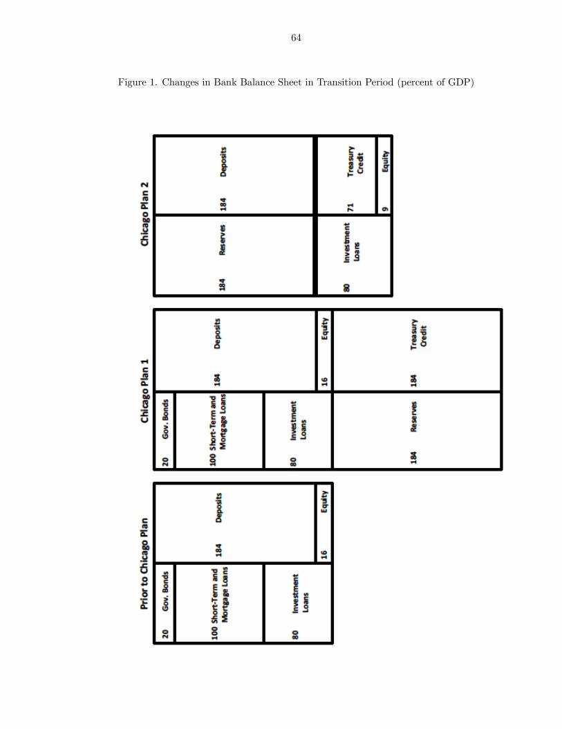
64

Figure 1. Changes in Bank Balance Sheet in Transition Period (percent of GDP)

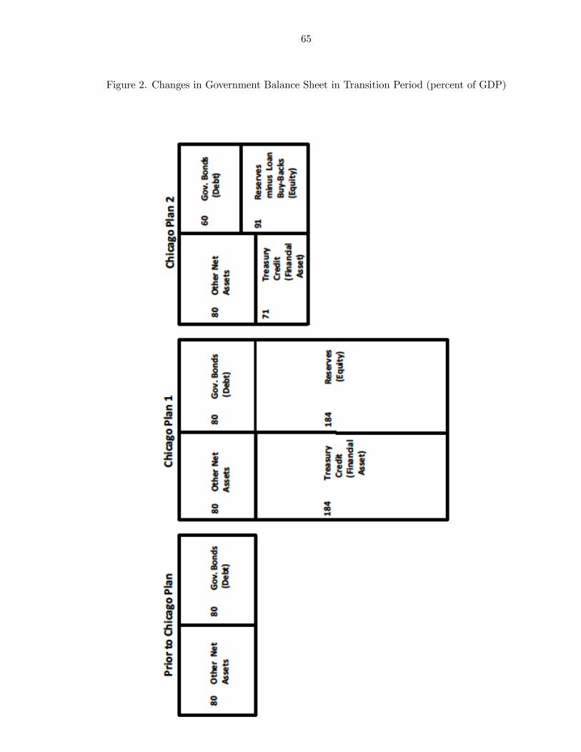
65

Figure 2. Changes in Government Balance Sheet in Transition Period (percent of GDP)

66

Figure 3. Changes in Bank Balance Sheet - Details (percent of GDP)

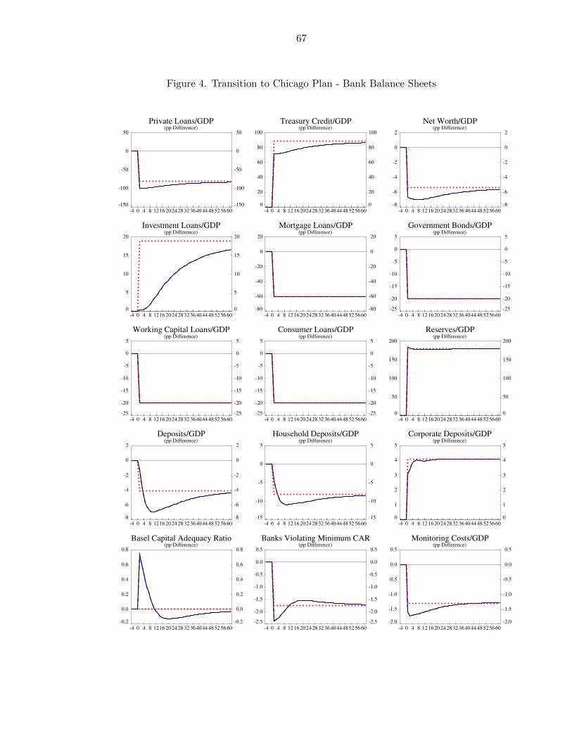
67

Figure 4. Transition to Chicago Plan - Bank Balance Sheets

-150

-100

-50

0

50

-150

-100

-50

0

50

-4 0 4 8 1216 20 24 28 32 3640 44 48 52 56 60

Private Loans/GDP(pp Difference)

0

20

40

60

80

100

0

20

40

60

80

100

-4 0 4 8 12 16 2024 28 32 36 40 4448 52 56 60

Treasury Credit/GDP(pp Difference)

-8

-6

-4

-2

0

2

-8

-6

-4

-2

0

2

-4 0 4 8 12 16 20 24 2832 36 40 44 48 5256 60

Net Worth/GDP(pp Difference)

0

5

10

15

20

0

5

10

15

20

-4 0 4 8 1216 20 24 28 32 3640 44 48 52 56 60

Investment Loans/GDP(pp Difference)

-80

-60

-40

-20

0

20

-80

-60

-40

-20

0

20

-4 0 4 8 12 16 2024 28 32 36 40 4448 52 56 60

Mortgage Loans/GDP(pp Difference)

-25

-20

-15

-10

-5

0

5

-25

-20

-15

-10

-5

0

5

-4 0 4 8 12 16 20 24 2832 36 40 44 48 5256 60

Government Bonds/GDP(pp Difference)

-25

-20

-15

-10

-5

0

5

-25

-20

-15

-10

-5

0

5

-4 0 4 8 1216 20 24 28 32 3640 44 48 52 56 60

Working Capital Loans/GDP(pp Difference)

-25

-20

-15

-10

-5

0

5

-25

-20

-15

-10

-5

0

5

-4 0 4 8 12 16 2024 28 32 36 40 4448 52 56 60

Consumer Loans/GDP(pp Difference)

0

50

100

150

200

0

50

100

150

200

-4 0 4 8 12 16 20 24 2832 36 40 44 48 5256 60

Reserves/GDP(pp Difference)

-8

-6

-4

-2

0

2

-8

-6

-4

-2

0

2

-4 0 4 8 1216 20 24 28 32 3640 44 48 52 56 60

Deposits/GDP(pp Difference)

-15

-10

-5

0

5

-15

-10

-5

0

5

-4 0 4 8 12 16 2024 28 32 36 40 4448 52 56 60

Household Deposits/GDP(pp Difference)

0

1

2

3

4

5

0

1

2

3

4

5

-4 0 4 8 12 16 20 24 2832 36 40 44 48 5256 60

Corporate Deposits/GDP(pp Difference)

-0.2

0.0

0.2

0.4

0.6

0.8

-0.2

0.0

0.2

0.4

0.6

0.8

-4 0 4 8 1216 20 24 28 32 3640 44 48 52 56 60

Basel Capital Adequacy Ratio(pp Difference)

-2.5

-2.0

-1.5

-1.0

-0.5

0.0

0.5

-2.5

-2.0

-1.5

-1.0

-0.5

0.0

0.5

-4 0 4 8 12 16 2024 28 32 36 40 4448 52 56 60

Banks Violating Minimum CAR(pp Difference)

-2.0

-1.5

-1.0

-0.5

0.0

0.5

-2.0

-1.5

-1.0

-0.5

0.0

0.5

-4 0 4 8 12 16 20 24 2832 36 40 44 48 5256 60

Monitoring Costs/GDP(pp Difference)

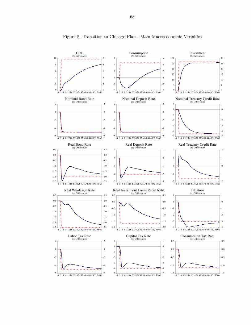
68

Figure 5. Transition to Chicago Plan - Main Macroeconomic Variables

0

2

4

6

8

10

0

2

4

6

8

10

-4 0 4 8 1216 20 24 28 32 3640 44 48 52 56 60

GDP(% Difference)

-4

-2

0

2

4

6

-4

-2

0

2

4

6

-4 0 4 8 12 16 2024 28 32 36 40 4448 52 56 60

Consumption(% Difference)

0

5

10

15

20

25

30

0

5

10

15

20

25

30

-4 0 4 8 12 16 20 24 2832 36 40 44 48 5256 60

Investment(% Difference)

-6

-4

-2

0

2

-6

-4

-2

0

2

-4 0 4 8 1216 20 24 28 32 3640 44 48 52 56 60

Nominal Bond Rate(pp Difference)

-6

-4

-2

0

2

-6

-4

-2

0

2

-4 0 4 8 12 16 2024 28 32 36 40 4448 52 56 60

Nominal Deposit Rate(pp Difference)

-5

-4

-3

-2

-1

0

1

-5

-4

-3

-2

-1

0

1

-4 0 4 8 12 16 20 24 2832 36 40 44 48 5256 60

Nominal Treasury Credit Rate(pp Difference)

-2.5

-2.0

-1.5

-1.0

-0.5

0.0

0.5

-2.5

-2.0

-1.5

-1.0

-0.5

0.0

0.5

-4 0 4 8 1216 20 24 28 32 3640 44 48 52 56 60

Real Bond Rate(pp Difference)

-3

-2

-1

0

1

-3

-2

-1

0

1

-4 0 4 8 12 16 2024 28 32 36 40 4448 52 56 60

Real Deposit Rate(pp Difference)

-2

-1

0

1

2

-2

-1

0

1

2

-4 0 4 8 12 16 20 24 2832 36 40 44 48 5256 60

Real Treasury Credit Rate(pp Difference)

-2.5

-2.0

-1.5

-1.0

-0.5

0.0

0.5

-2.5

-2.0

-1.5

-1.0

-0.5

0.0

0.5

-4 0 4 8 1216 20 24 28 32 3640 44 48 52 56 60

Real Wholesale Rate(pp Difference)

-2.0

-1.5

-1.0

-0.5

0.0

0.5

-2.0

-1.5

-1.0

-0.5

0.0

0.5

-4 0 4 8 12 16 2024 28 32 36 40 4448 52 56 60

Real Investment Loans Retail Rate(pp Difference)

-4

-3

-2

-1

0

1

-4

-3

-2

-1

0

1

-4 0 4 8 12 16 20 24 2832 36 40 44 48 5256 60

Inflation(pp Difference)

-6

-4

-2

0

2

-6

-4

-2

0

2

-4 0 4 8 1216 20 24 28 32 3640 44 48 52 56 60

Labor Tax Rate(pp Difference)

-5

-4

-3

-2

-1

0

1

-5

-4

-3

-2

-1

0

1

-4 0 4 8 12 16 2024 28 32 36 40 4448 52 56 60

Capital Tax Rate(pp Difference)

-1.5

-1.0

-0.5

0.0

0.5

-1.5

-1.0

-0.5

0.0

0.5

-4 0 4 8 12 16 20 24 2832 36 40 44 48 5256 60

Consumption Tax Rate(pp Difference)

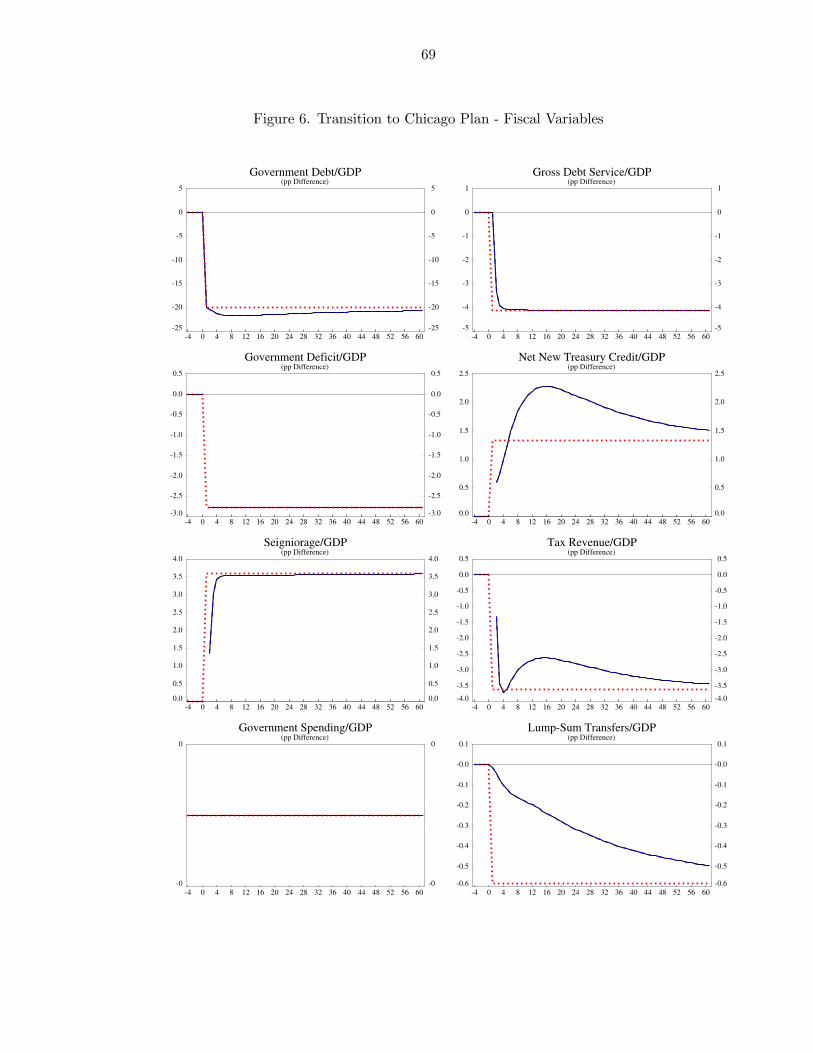
69

Figure 6. Transition to Chicago Plan - Fiscal Variables

-25

-20

-15

-10

-5

0

5

-25

-20

-15

-10

-5

0

5

-4 0 4 8 12 16 20 24 28 32 36 40 44 48 52 56 60

Government Debt/GDP(pp Difference)

-5

-4

-3

-2

-1

0

1

-5

-4

-3

-2

-1

0

1

-4 0 4 8 12 16 20 24 28 32 36 40 44 48 52 56 60

Gross Debt Service/GDP(pp Difference)

-3.0

-2.5

-2.0

-1.5

-1.0

-0.5

0.0

0.5

-3.0

-2.5

-2.0

-1.5

-1.0

-0.5

0.0

0.5

-4 0 4 8 12 16 20 24 28 32 36 40 44 48 52 56 60

Government Deficit/GDP(pp Difference)

0.0

0.5

1.0

1.5

2.0

2.5

0.0

0.5

1.0

1.5

2.0

2.5

-4 0 4 8 12 16 20 24 28 32 36 40 44 48 52 56 60

Net New Treasury Credit/GDP(pp Difference)

0.0

0.5

1.0

1.5

2.0

2.5

3.0

3.5

4.0

0.0

0.5

1.0

1.5

2.0

2.5

3.0

3.5

4.0

-4 0 4 8 12 16 20 24 28 32 36 40 44 48 52 56 60

Seigniorage/GDP(pp Difference)

-4.0

-3.5

-3.0

-2.5

-2.0

-1.5

-1.0

-0.5

0.0

0.5

-4.0

-3.5

-3.0

-2.5

-2.0

-1.5

-1.0

-0.5

0.0

0.5

-4 0 4 8 12 16 20 24 28 32 36 40 44 48 52 56 60

Tax Revenue/GDP(pp Difference)

-0

0

-0

0

-4 0 4 8 12 16 20 24 28 32 36 40 44 48 52 56 60

Government Spending/GDP(pp Difference)

-0.6

-0.5

-0.4

-0.3

-0.2

-0.1

-0.0

0.1

-0.6

-0.5

-0.4

-0.3

-0.2

-0.1

-0.0

0.1

-4 0 4 8 12 16 20 24 28 32 36 40 44 48 52 56 60

Lump-Sum Transfers/GDP(pp Difference)

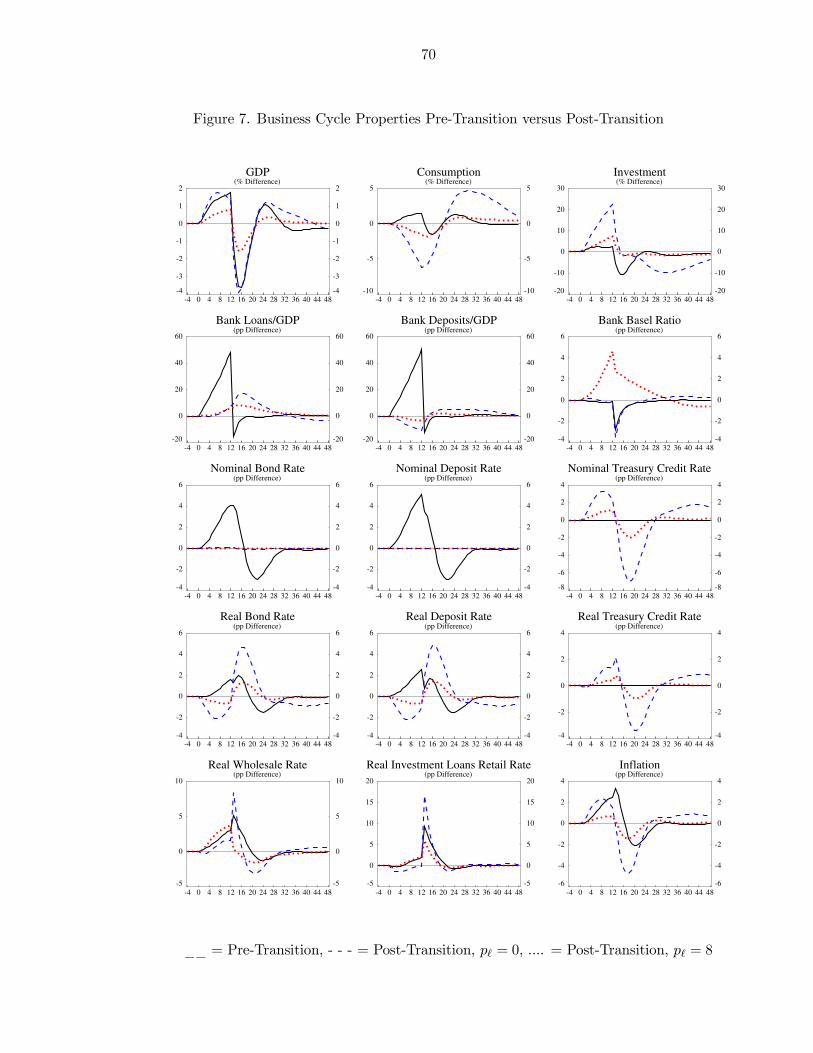
70

Figure 7. Business Cycle Properties Pre-Transition versus Post-Transition

-4

-3

-2

-1

0

1

2

-4

-3

-2

-1

0

1

2

-4 0 4 8 12 16 20 24 28 32 36 40 44 48

GDP(% Difference)

-10

-5

0

5

-10

-5

0

5

-4 0 4 8 12 16 20 24 28 32 36 40 44 48

Consumption(% Difference)

-20

-10

0

10

20

30

-20

-10

0

10

20

30

-4 0 4 8 12 16 20 24 28 32 36 40 44 48

Investment(% Difference)

-20

0

20

40

60

-20

0

20

40

60

-4 0 4 8 12 16 20 24 28 32 36 40 44 48

Bank Loans/GDP(pp Difference)

-20

0

20

40

60

-20

0

20

40

60

-4 0 4 8 12 16 20 24 28 32 36 40 44 48

Bank Deposits/GDP(pp Difference)

-4

-2

0

2

4

6

-4

-2

0

2

4

6

-4 0 4 8 12 16 20 24 28 32 36 40 44 48

Bank Basel Ratio(pp Difference)

-4

-2

0

2

4

6

-4

-2

0

2

4

6

-4 0 4 8 12 16 20 24 28 32 36 40 44 48

Nominal Bond Rate(pp Difference)

-4

-2

0

2

4

6

-4

-2

0

2

4

6

-4 0 4 8 12 16 20 24 28 32 36 40 44 48

Nominal Deposit Rate(pp Difference)

-8

-6

-4

-2

0

2

4

-8

-6

-4

-2

0

2

4

-4 0 4 8 12 16 20 24 28 32 36 40 44 48

Nominal Treasury Credit Rate(pp Difference)

-4

-2

0

2

4

6

-4

-2

0

2

4

6

-4 0 4 8 12 16 20 24 28 32 36 40 44 48

Real Bond Rate(pp Difference)

-4

-2

0

2

4

6

-4

-2

0

2

4

6

-4 0 4 8 12 16 20 24 28 32 36 40 44 48

Real Deposit Rate(pp Difference)

-4

-2

0

2

4

-4

-2

0

2

4

-4 0 4 8 12 16 20 24 28 32 36 40 44 48

Real Treasury Credit Rate(pp Difference)

-5

0

5

10

-5

0

5

10

-4 0 4 8 12 16 20 24 28 32 36 40 44 48

Real Wholesale Rate(pp Difference)

-5

0

5

10

15

20

-5

0

5

10

15

20

-4 0 4 8 12 16 20 24 28 32 36 40 44 48

Real Investment Loans Retail Rate(pp Difference)

-6

-4

-2

0

2

4

-6

-4

-2

0

2

4

-4 0 4 8 12 16 20 24 28 32 36 40 44 48

Inflation(pp Difference)

__ = Pre-Transition, - - - = Post-Transition, pℓ = 0, .... = Post-Transition, pℓ = 8