Embed Size (px)
Citation preview

J Optim Theory Appl (2013) 157:148–167DOI 10.1007/s10957-012-0159-6
The Chebyshev–Shamanskii Method for SolvingSystems of Nonlinear Equations
Bilel Kchouk · Jean-Pierre Dussault
Received: 22 December 2011 / Accepted: 9 August 2012 / Published online: 31 August 2012© Springer Science+Business Media, LLC 2012
Abstract We present a method, based on the Chebyshev third-order algorithm andaccelerated by a Shamanskii-like process, for solving nonlinear systems of equations.We show that this new method has a quintic convergence order. We will also focuson efficiency of high-order methods and more precisely on our new Chebyshev–Shamanskii method. We also identify the optimal use of the same Jacobian in theShamanskii process applied to the Chebyshev method. Some numerical illustrationswill confirm our theoretical analysis.
Keywords Newton method · Chebyshev method · Shamanskii process · Algorithmefficiency · Automatic differentiation
1 Introduction
In this paper, we introduce a method to solve nonlinear systems of equations, com-bining a good convergence order from the Chebyshev method and higher efficiencyfrom the Shamanskii process. This method is also relevant for nonlinear and differ-entiable optimization problems as for variational inequality problems. Actually wepresent our main developments for symmetric systems arising from unconstrained
Communicated by Jean-Pierre Crouzeix.
B. Kchouk (�)Department of Mathematics, University of Sherbrooke, 2500 Bvd de l’Université,J1K2R1 Sherbrooke, QC, Canadae-mail: [email protected]
J.-P. DussaultDepartment of Computer Science, University of Sherbrooke, 2500 Bvd de l’Université,J1K2R1 Sherbrooke, QC, Canadae-mail: [email protected]

J Optim Theory Appl (2013) 157:148–167 149
optimization, and moreover we selected all our test functions from an unconstrainedoptimization library [1].
In 1838, Chebyshev developed a (high-order) method with a local cubic conver-gence, improving the well-known Newton method [2] which converges quadratically.The Chebyshev method [3] shares this cubic-order of convergence with other well-known methods, such as Halley [4] and SuperHalley [5]. However the Chebyshevmethod differs from these two by the fact that one iteration needs the inversion ofone matrix, whereas the Halley and SuperHalley methods require the inversion oftwo different matrices. This constitutes a first important aspect of our research.
Some authors have studied the Chebyshev method trying to improve its behavior.In particular, in [6], the authors introduced a method similar to Chebyshev, whileavoiding to compute the second derivative. We believe, as described later, that thiscomputation does not constitute a major challenge. In [7] and [8], the authors pre-sented an improvement of the region of accessibility of the Chebyshev method (orother cubical methods). This is an important aspect of the research on high-ordermethods that we do not address in this work. Nevertheless, this should be the subjectof a forthcoming research. In this paper, we focus on a new method which improvesthe local convergence order of the Chebyshev method without increasing substan-tially its complexity.
Indeed, high-order methods involve high-order derivatives. We consider a tech-nique which allows one to save on costs of high-order methods: automatic differen-tiation [9]. By detailing the various costs of obtaining the derivatives, we will showthat the main complexity of such algorithms comes from the inversion of the Jacobianmatrix, and not from obtaining higher-order derivatives. In this sense, the Chebyshevmethod is more interesting than that of Halley and SuperHalley. In [10] the authoralso used the automatic differentiation to estimate the computational cost of high-order algorithms. He studied the Chebyshev, Halley and SuperHalley methods usingthis tool. However, his theoretical estimates for high-order methods’ complexities canbe improved, and his analysis could be extended to other methods, as we will presentit in this paper.
The second interest of the Chebyshev algorithm, which inverts only one matrix,comes from the idea of Shamanskii [11]. In 1967, Shamanskii introduced an accel-eration for Newton’s method by a pseudo-Newton step re-using the same Jacobianmatrix as in the previous iteration. In fact, from a quadratically convergent method heobtained a cubic convergence result that competes seriously with the Halley, Cheby-shev and SuperHalley methods. Actually, in [12], the authors give credit to Traub [13]for this result he published in 1964. They also recognize that Shamanskii (also writ-ten Šamanskii) developed an extended version of this result. Nevertheless, as Kelleydid in [14], we adopt the convention to name this method as the Shamanskii method.Some authors, as Lampariello [15] and Brent [16], developed an extension of thisprocess. In particular, Brent used the efficiency index introduced by Ostrowski [17]to assess the number of iterations that we should reuse the same Jacobian.
Ezquerro et al. [18] have recently exploited the idea of such an acceleration. How-ever, their algorithm does not reuse the same Jacobian matrix. The authors considerthat the main cost of such high-order methods comes from obtaining high-orderderivatives, and their idea is to update the tensor every two iterations, and not the

150 J Optim Theory Appl (2013) 157:148–167
inverse Jacobian. We will show that, on the opposite, by computing subtly differentterms, it is indeed the inversion of the Jacobian that is the most expensive task, moreexpensive than obtaining the higher-order information.
Among recent research on higher-order methods, Gundersen and Steihaug pub-lished their results in [19]. They developed specific ways to exploit sparsity in ma-trices and higher-order tensors. We pursue a different path avoiding explicit use oftensors. Furthermore, they do not take into account the full cost of a method, as wedo in this paper. As a matter of fact, their analysis is based on intrinsic complexi-ties of algorithms, without considering the costs of computing the function and itsderivatives.
Thus, the goal of this paper is to introduce the Chebysev–Shamanskii method,prove its quintic-order of convergence, and show that it does not cost significantlymore than the Chebyshev or Newton methods. Thus, we improve the efficiency ofthe Chebyshev method by accelerating it with a Shamanskii process. Moreover, wediscuss how to apply the Shamanskii acceleration to other high-order methods, inparticular to high-order Chebyshev directions [20].
This paper is organized as follows: in Sect. 2, we will recall the High-order Cheby-shev (HoC) methods and discuss the costs and efficiencies of algorithms in order tochoose a useful index to compare optimization methods. In the Sect. 3, we will intro-duce the Chebyshev–Shamanskii method, first by emphasizing the major usefulnessof the Shamanskii process; i.e. how to optimally use the idea of Shamankii accel-eration, while considering the highest cost in a Newton-type method. Thus, we willpresent our main result: the order of convergence of the method and its cost comparedto Chebyshev method and, more generally, convergence of any method acceleratedby a similar process.
Section 4 will illustrate our method on examples and therefore emphasize ourtheoretical results.
In Sect. 5, as Brent [16] did for the Newton method, we will see how many timeswe should use the same Jacobian in this Chebyshev–Shamanskii method, i.e. afterhow many reuse of this matrix we should update it.
2 Preliminaries
In this section, we will first give a brief reminder on the High-order Chebyshev meth-ods and then discuss the notion of an algorithm cost and efficiency. First, for thereader’s convenience, we present some hypothesis, which will be used throughoutthis article.
2.1 Notation
We define an open ball S centered on a root x∗ of F (i.e. F(x∗) = 0), S = S(x∗, δ) ⊂D ⊂ R
n, for a certain δ > 0.
• H1(p): F : D ⊂ Rn → R
n is p-Fréchet-differentiable in S;• H2: F satisfies ‖∇F(x) − ∇F(x∗)‖ ≤ α‖x − x∗‖ ∀x ∈ S;• H3: F(x∗) = 0, and ∇F(x∗) is non-singular.

J Optim Theory Appl (2013) 157:148–167 151
Moreover the following notations are chosen:
• dN,dC will refer respectively to Newton’s and Chebyshev’s directions, i.e.,dN = −∇F(x)−1F(x) and dC = dN − 1
2∇F(x)−1∇2F(x)dNdN ;
• ∇2F(x)u = (∑n
j=1∂2F(x)∂xi∂xj
uj ) ∈ Rn×n;
• ∇2F(x)uv = ((∇2F(x)u)v) ∈ Rn.
When F(x) = ∇f (x), the system corresponds to the first-order necessary optimalityconditions for the problem minf (x). In this case, ∇F(x∗) = ∇2f (x∗) is symmetric,and we assume that it is positive definite. We present a detailed analysis using theCholesky factorization of ∇F(x). The arithmetic complexity of the Cholesky factor-ization is ( 1
3n3 + 12n2 − 5
6n) according to [21]. For unsymmetric systems, we assumethat ∇F(x∗) is an invertible matrix, and the PLU factorization with partial pivotingof complexity ( 2
3n3 − 12n2 − 1
6n) could be used. We give a similar analysis for unsym-metric systems in Appendix B. It is easy to see that all our comparisons and resultsremain valid for unsymmetric systems.
2.2 High-Order Chebyshev Methods
In [20], we presented a family of high-order directions dM (High-order Cheby-shev directions, abbreviated by HoC) leading to an iterative algorithm defined byxk+1 = x + dM . Newton, Chebyshev, and J.-P. Dussault’s extrapolations [22] obeythis definition. These directions are defined, in practice, by the following scheme:
F(xk) + ∇F(xk)D + 1
2∇2F(xk)d1d2 + · · · + 1
p!∇pF (xk) dl dl+1 . . . dl+p−1 = 0,
(1)
where l = p(p−1)2 , and di , i = 1, . . . , l + p − 1, are linear combinations of directions
defined by the same scheme but at a lower-order. Therefore, we expect a p-orderdirection (HoC(p)) to have a p + 1 convergence order.
As a matter of fact, these HoC directions have a high order of convergence with-out increasing significantly the algorithmic cost of computation. In other words, HoCmethods improve efficiencies of well-known methods (such as Chebyshev and New-ton) when the higher-order terms are evaluated efficiently. Baur and Strassen [23]set the theoretical bounds for obtaining the derivatives of some real-valued functionφ : R
n → R: cost(∇φ) ≤ 4 cost(φ). Using automatic differentiation (AD), one canrely on the availability of a gradient ∇φ at a computational cost at worst five timesthe cost of computing φ itself, and the factor is very conservative. We also referto [24] for a more detailed analysis. Actually cost(∇φ +φ) ≤ 5 cost(φ). This is com-petitive with carefully hand-coded gradients. We use this complexity bound to assessthe overall complexity of our HoC algorithm. Actually, as described in [25], obtain-ing ∇F may cost n times the cost of F for a vector-valued function F : R
n → Rn.
In contrast, to compute the vector quantity ∇F(x)u (u ∈ Rn), we should express
it as ∇(F (x)u), i.e. the derivative of a the scalar valued function Φ : x → F(x)u;and obtaining ∇F(x)u costs, again at worst five times the cost of computing F(x)u.The same clever idea is used to compute ∇2F(x)uv considered as ∇(∇(F (x)u)v)
152 J Optim Theory Appl (2013) 157:148–167
(v ∈ Rn); thus this quantity will cost no more than five times the cost of ∇(F (x)u)v
considered as a dot product of ∇F(x)u and v. And so on for ∇3F(x)uvw etc.
2.3 Algorithm Cost and Efficiency
The previous analysis concerns one aspect of the cost of an algorithm, which is ob-taining high-order derivatives. Actually, the cost of an algorithm depends on threecomplexities:
1. The cost (c) of evaluating F . As F : D ⊂ Rn → R
n, c n(cost(fi)), i = 1, . . . , n,where fi(x) = ∂F (x)
∂xi. In practice, c = O(nq) where q ≤ 3. We will develop this
estimation in Sect. 4.2. The cost of obtaining the derivative ∇F(x), ∇F(x)u, ∇2F(x)uv (where u,
v ∈ Rn), etc.
3. The intrinsic algorithmic computation complexity of a method.
Many authors base their calculations only on estimates of the third cost of the pre-vious list (see for example [19]). Some others consider the algorithmic cost (3) andthe cost of obtaining derivative (2) (see for example [18]), but generally they omit toconsider a cheaper way to compute these derivatives (such as AD). Therefore their
estimates are biased as the main cost comes from the inversion of ∇F(x) ( n3
3 ) andnot from obtaining higher-order derivatives, since they can be considered as a productof Hessian (or tensor) and vectors as described above.
We here present an approach taking into account the overall complexity of analgorithm, i.e. the three previous costs. As in [10], we use AD to obtain higher-orderderivative and estimate complexity of our method, but as in [20], we improve theseestimations and compute more specifically our method’s complexity.
In addition, we here reuse the efficiency index developed in [20]. Brent in [16] andEzquerro et al. [18] refer to Ostrowski [17] to define such an efficiency. But we insistthat they do not consider the global cost of a method, and consequently their indexdoes not faithfully reflect a method’s efficiency. Thus, we define the efficiency indexused throughout this paper as
E(M) := log(conv(M))
C(M),
where C(M) is the total cost of one iteration of the method M , and conv(M) theconvergence order of this method. In Table 1, we give details concerning the cost ofeach operation.
Knowing these costs, one can evaluate Newton and Chebyshev direction’s com-plexity:
• Newton’s direction expressed as dN = −∇F(xk)−1F(xk) has the cost
C(dN) = 1
3n3 + 5
2n2 − 5
6n + (n + 1)c.
• To compute Chebyshev’s direction, first compute Newton’s direction;

J Optim Theory Appl (2013) 157:148–167 153
Table 1 Costs of operationsinvolved in high-order methods Operation Cost
Cholesky factorization [21] 13 n3 + 1
2 n2 − 56 n
Solving linear system 2n2 − n
Cost of F c
Obtaining derivative ∇F(xk) with AD [9] nc
∇F(xk)u = ∇(F (xk)u) where u ∈ Rn [25] 5c + 5n
∇2F(xk)uv = ∇(∇(F (xk)u)v) where u,v ∈ Rn 25c + 30n
Vector subtraction or sum n
dC = dN − 12∇F(xk)
−1∇2F(xk)dNdN . Thus, its cost is at most
C(dC) = 1
3n3 + 9
2n2 + 181
6n + (n + 26)c.
Consequently, the efficiency of the Newton method is
E(dN) = log(2)
13n3 + 5
2n2 − 56n + (n + 1)c
,
and the efficiency of the Chebyshev method is
E(dC) = log(3)
13n3 + 9
2n2 + 1816 n + (n + 26)c
.
Having all this information, we can now introduce our Chebyshev–Shamanskiimethod.
3 Chebyshev–Shamanskii Method
It is known that, sufficiently close to a root, the Newton method has a quadratic con-vergence order [2] and the Chebyshev method converges cubically [3]. But as seenbefore, the additional complexity of the Chebyshev method compared to Newton’sis (2n2 + 31n + 25c), in other words, O(n2) as long as c = O(n2) (c being thecost of evaluating F(x)), whereas the dominant term in both Newton and Chebyshev
methods is ( n3
3 ) coming from the Cholesky factorization of the Jacobian matrix. Inthe case where this cost is higher (for example c = O(n3)), the Newton and Cheby-shev methods will have the same complexity O(nc). Therefore, the main idea ofthe Chebyshev–Shamanskii method is to improve the convergence of the Chebyshevmethod by using the Shamanskii process to limit the overall complexity.
3.1 Main Interest of Shamanskii Process
In 1967, Shamanskii [11] developed a multiple pseudo-Newton iteration method de-scribed by
xk+ 1
2= xk − ∇F(xk)
−1F(xk),

154 J Optim Theory Appl (2013) 157:148–167
xk+1 = xk+ 1
2− ∇F(xk)
−1F(xk+ 1
2).
This is equivalent to
xk+1 = xk − ∇F(xk)−1[F(xk) + F
(xk − ∇F(xk)
−1F(xk))]
. (2)
This method is known to be efficient in terms of complexity as it uses only one Jaco-bian for two pseudo-Newton iterations, i.e. the additional cost of Shamanskii methodcompared to Newton’s is only (2n2 +c), which corresponds to one resolution of a lin-ear system, one evaluation of F(x) and one vectorial subtraction. The convergenceof this method has been demonstrated.
Theorem 3.1 [12] Let F : D ⊂ Rn → R
n obey hypotheses H1(2), H2, and H3. Thenx∗ is a point of attraction of the Shamanskii iteration (i.e., Eq. (2)), and this iterativemethod has an order of convergence at least cubical.
Several authors studied the Shamanskii method and its technique. For example, werefer to [12, 13, 15, 16]. In [18], the authors present a similar technique to enforce theconvergence of any iterative algorithm and more particularly the super-Halley method[5]. Their result can be summarized as follows: if zk := xk + φ(xk) is an iterativemethod converging at a ρ-order, then if we define dN(zk) := −∇F(zk)
−1F(zk), thenew iterative method defined by
xk+1 := zk + dN(zk) − 1
2∇F(zk)
−1∇2F(xk)dN(zk)dN(zk)
converges at a (2ρ +1)-order. Here, two observations should be underlined. First, onewonders why reuse the same tensor (∇2F(x)). According to the authors’ analysis, themain complexity of such a method comes from obtaining this tensor, and therefore weshould use it more than once (twice is this case). However, as explained before, it isnot necessary to compute (∇2F(x)) (which costs O(n3) according to the authors, andmore precisely O(cn2) as we should take into account obtaining of F(x)). It makesmore sense to compute ∇2F(x)dNdN which will cost “only” (25c + 30n) (which isa worst-case bound and quite pessimistic).
Therefore, reusing the same tensor does not seem relevant as its cost is generallylower than the inversion of the Jacobian. As a matter of fact, it is easy to show that byadding a classical Chebyshev step to a method converging at a (ρ)-order, we wouldhave a new (3ρ) convergence order method. In other words, the method presented in
[18] actually costs O( n3
3 + cn2) for a (2ρ + 1)-order of convergence, whereas a full
second Chebyshev step would cost O( n3
3 + cn) for a (3ρ)-order of convergence.Thus, the second remark concerns this inverse Jacobian (∇F(x)−1). The authors
update this matrix each new calculus, losing the entire gain from Shamanskii’s idea.Indeed, with Shamanskii’s process, we avoid the main complexity (Cholesky factor-ization) by reusing the same Jacobian. This should be the basic idea of a Shamanskii-like method.

J Optim Theory Appl (2013) 157:148–167 155
3.2 Main Result
As explained in [20], one needs to choose carefully the directions di to be injectedinto equation (1) in order to define a new HoC direction having good convergenceproperties. Then, the main idea of this paper is to accelerate Chebyshev algorithm bya Shamanskii-like process, in order to improve its convergence without significantlyincreasing its complexity, i.e. to improve its efficiency.
First we consider a general two-step iterative algorithm⎧⎪⎪⎪⎪⎨
⎪⎪⎪⎪⎩
yk := xk + Φ(xk),
dNk:= −∇F(xk)
−1F(xk),
dNk:= −∇F(xk)
−1F(yk),
xk+1 := yk + dNk− 1
2∇F(xk)−1∇2F(yk)dNk
(2dNk),
(3)
where Φ : Rn → R
n defines an iterative method. An example of this two-step processis what we define as the Chebyshev–Shamanskii algorithm.
Definition 3.1 The Chebyshev–Shamanskii method is defined by{
yk := xk + dCk,
xk+1 := yk + dNk− 1
2∇F(xk)−1∇2F(yk)dNk
(2dNk),
(4)
where dCkand dNk
are the classical Chebyshev and Newton directions applied to xk ,and dNk
is a pseudo-Newton step, i.e.
⎧⎪⎨
⎪⎩
dNk:= −∇F(xk)
−1F(xk),
dCk:= dNk
− 12∇F(xk)
−1∇2F(xk)dNkdNk
,
dNk:= −∇F(xk)
−1F(yk).
Remark 3.1 Notice the (2dNk) term. As analyzed in [20], the directions transformed
by ∇2F need to be carefully chosen to obtain high convergence order, and in our
case, the directions allowing one to prove quintic-order are dNkand 2dNk
.
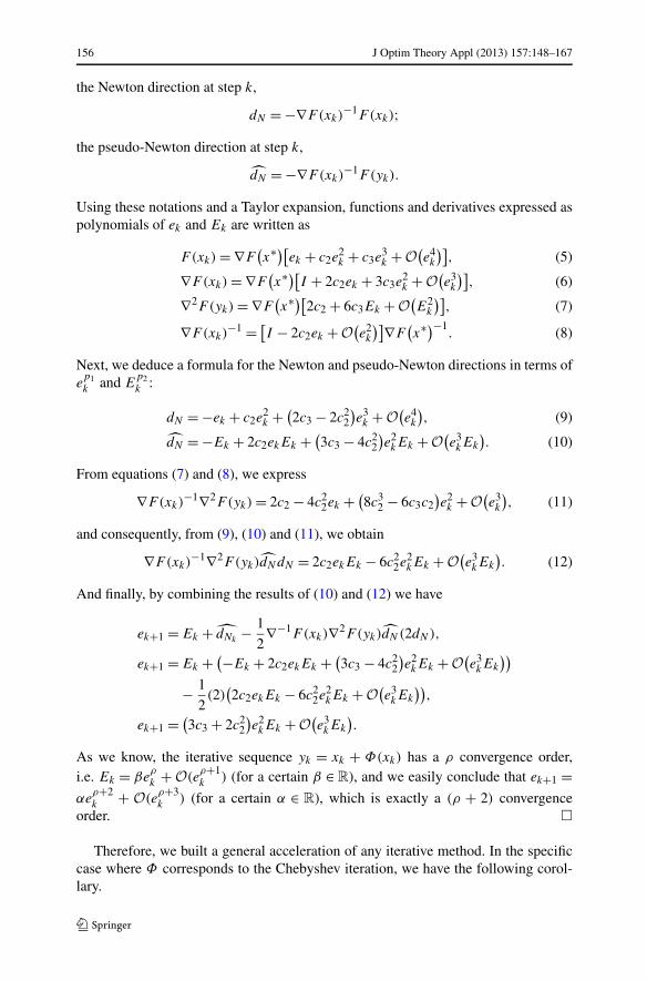
Theorem 3.2 Under assumptions H1(2), H2 and H3, if the local order of conver-gence of the iterative sequence defined by Φ is ρ, then the sequence (3) convergesto x∗ (with F(x∗) = 0) with at least a (ρ + 2) local convergence order.
Proof Assuming hypotheses H1(2), H2 and H3, we first define the error steps ek :=xk − x∗; Ek := yk − x∗ and ek+1 := xk+1 − x∗. Therefore, having
F(x∗) = 0,
we define several quantities. First, a useful coefficient
ck = 1
k!∇F(x∗)−1∇kF
(x∗);
156 J Optim Theory Appl (2013) 157:148–167
the Newton direction at step k,
dN = −∇F(xk)−1F(xk);
the pseudo-Newton direction at step k,
dN = −∇F(xk)−1F(yk).
Using these notations and a Taylor expansion, functions and derivatives expressed aspolynomials of ek and Ek are written as
F(xk) = ∇F(x∗)[ek + c2e
2k + c3e
3k + O
(e4k
)], (5)
∇F(xk) = ∇F(x∗)[I + 2c2ek + 3c3e
2k + O
(e3k
)], (6)
∇2F(yk) = ∇F(x∗)[2c2 + 6c3Ek + O
(E2
k
)], (7)
∇F(xk)−1 = [
I − 2c2ek + O(e2k
)]∇F(x∗)−1
. (8)
Next, we deduce a formula for the Newton and pseudo-Newton directions in terms ofep1k and E
p2k :
dN = −ek + c2e2k + (
2c3 − 2c22
)e3k + O
(e4k
), (9)
dN = −Ek + 2c2ekEk + (3c3 − 4c2
2
)e2kEk + O
(e3kEk
). (10)
From equations (7) and (8), we express
∇F(xk)−1∇2F(yk) = 2c2 − 4c2
2ek + (8c3
2 − 6c3c2)e2k + O
(e3k
), (11)
and consequently, from (9), (10) and (11), we obtain
∇F(xk)−1∇2F(yk)dNdN = 2c2ekEk − 6c2
2e2kEk + O
(e3kEk
). (12)
And finally, by combining the results of (10) and (12) we have
ek+1 = Ek + dNk− 1
2∇−1F(xk)∇2F(yk)dN (2dN),
ek+1 = Ek + (−Ek + 2c2ekEk + (3c3 − 4c2
2
)e2kEk + O
(e3kEk
))
− 1
2(2)
(2c2ekEk − 6c2
2e2kEk + O
(e3kEk
)),
ek+1 = (3c3 + 2c2
2
)e2kEk + O
(e3kEk
).
As we know, the iterative sequence yk = xk + Φ(xk) has a ρ convergence order,i.e. Ek = βe
ρk + O(e
ρ+1k ) (for a certain β ∈ R), and we easily conclude that ek+1 =
αeρ+2k + O(e
ρ+3k ) (for a certain α ∈ R), which is exactly a (ρ + 2) convergence
order. �
Therefore, we built a general acceleration of any iterative method. In the specificcase where Φ corresponds to the Chebyshev iteration, we have the following corol-lary.

J Optim Theory Appl (2013) 157:148–167 157
Corollary 3.1 Under assumptions H1(2), H2 and H3, the iterative method defined inEq. (4) converges to x∗ (with F(x∗) = 0) with at least a quintic convergence order.The additional complexity of such a method compared to Chebyshev is 4n2 + 26c +30n (with c being the cost of evaluating F(x)).
Proof The convergence result is obvious when one takes ρ = 3. Referring to resultsof the section Algorithm Cost and Efficiency (p. (152)), we can easily verify that theChebyshev–Shamanskii method requires (compared to the first Chebyshev step): twolinear systems to be solved (costing 4n2 − 2n), one evaluation of ∇2F(x)uv (costing25c + 30n) (u, v being in R
n), one evaluation of F (costing c) at the point yk , andfinally the sum of two vectors (costing 2n), the total being (4n2 + 26c + 30n). �
4 Numerical Experiments
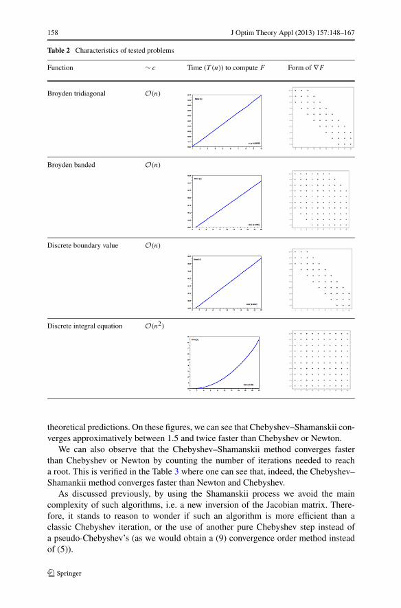
In this section, we illustrate the theoretical results presented above. We considerfour examples of functions (f ) taken from the collection of Moré, Garbow and Hill-strom [1], selected in order to vary the sizes of problems, and costs of evaluations.We present in the Table 2 some aspects of each function.
In the second column, we present the overall approximation of the cost of evalu-ation of F(x) = ∇f (x). In the third column, we show the time needed to computeF relatively to the size of the problem. The aspect of these graphics corresponds toour predictions in terms of global cost, i.e. the complexity of F is indeed O(n2) orO(n). The last column shows the general form of the matrix ∇F . We observe thatthe cost of obtaining F is generally related to the structure of the matrix ∇F . Whenthis matrix is banded, we expect the cost of F to be linear in terms of the size n;whereas for a full matrix ∇F , this cost of obtaining F is around O(n2). The detailsfor these functions and their hand-computed costs are given in Appendix A. As in[10], we do not consider the special structures (i.e. sparsity in matrices) in our algo-rithms.
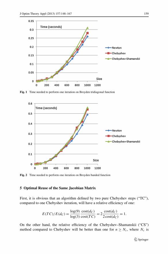
We also want to confirm that one iteration of Chebyshev–Shamanskii, Cheby-shev and Newton share approximately the same complexity. A good indicator isthe time needed to perform one iteration. Therefore, the four following graph-ics (Figs. 1, 2, 3, and 4) illustrate this result: all these methods have a complex-ity around ( 1
3n3 + nc). (We refer to the preliminary analysis in Sect. 2.3 and toCorollary 3.1). If c = O(n), as in (Figs. 1–3) then the total cost of a methodM is approximated by ( 1
3n3 + βMn2), where βM is a constant depending on themethod. In contrast, if c = O(n2) (as in Fig. 4), then the total cost of all thesemethods is approximated by βn3, where β does not depend on a method. Weeasily conclude that for bigger-sized problems, the dominant term being O(n3),all these methods have quite the same behavior in terms of time for one itera-tion.
The Chebyshev–Shamanskii method has about the same complexity (or time) asthe Newton or Chebyshev methods. The crucial question concerns its general be-havior, i.e.: does Chebyshev–Shamanskii converge faster than Chebyshev (and con-sequently Newton)? The following graphics (Figs. 5, 6, 7, and 8) confirm, also, our
158 J Optim Theory Appl (2013) 157:148–167
Table 2 Characteristics of tested problems
Function ∼ c Time (T (n)) to compute F Form of ∇F
Broyden tridiagonal O(n)
Broyden banded O(n)
Discrete boundary value O(n)
Discrete integral equation O(n2)
theoretical predictions. On these figures, we can see that Chebyshev–Shamanskii con-verges approximatively between 1.5 and twice faster than Chebyshev or Newton.
We can also observe that the Chebyshev–Shamanskii method converges fasterthan Chebyshev or Newton by counting the number of iterations needed to reacha root. This is verified in the Table 3 where one can see that, indeed, the Chebyshev–Shamankii method converges faster than Newton and Chebyshev.
As discussed previously, by using the Shamanskii process we avoid the maincomplexity of such algorithms, i.e. a new inversion of the Jacobian matrix. There-fore, it stands to reason to wonder if such an algorithm is more efficient than aclassic Chebyshev iteration, or the use of another pure Chebyshev step instead ofa pseudo-Chebyshev’s (as we would obtain a (9) convergence order method insteadof (5)).
J Optim Theory Appl (2013) 157:148–167 159
Fig. 1 Time needed to perform one iteration on Broyden tridiagonal function
Fig. 2 Time needed to perform one iteration on Broyden banded function
5 Optimal Reuse of the Same Jacobian Matrix
First, it is obvious that an algorithm defined by two pure Chebyshev steps (“TC”),compared to one Chebyshev iteration, will have a relative efficiency of one:
E(T C)/E(dC) = log(9)
log(3)
cost(dC)
cost(T C)= 2
cost(dC)
2 cost(dC)= 1.
On the other hand, the relative efficiency of the Chebyshev–Shamanskii (“CS”)method compared to Chebyshev will be better than one for n ≥ Nc, where Nc is

160 J Optim Theory Appl (2013) 157:148–167
Fig. 3 Time needed to perform one iteration on Discrete boundary value function
Fig. 4 Time needed to perform one iteration on Discrete integral equation function
an integer which depends on c. As a matter of fact,
E(CS)/E(dC) = log(5)
log(3)
cost(dC)
cost(CS)
= log(5)
log(3)
cost(dC)
cost(dC) + 4n2 + 26c + 30n
= log(5)
log(3)
13n3 + 9
2n2 + 1816 n + (n + 26)c
cost(dC) + 4n2 + 26c + 30n.
If we approximate c by n2, then E(CS)/E(dC) ≥ 1 for n ≥ 25; and if c = n3, thenE(CS)/E(dC) ≥ 1 for n ≥ 30. In other words, the Chebyshev–Shamanskii algorithmis more beneficial compared to a classical Chebyshev method for n ≥ 30 in general.

J Optim Theory Appl (2013) 157:148–167 161
Fig. 5 Time needed to converge to a root on Broyden tridiagonal function
Fig. 6 Time needed to converge to a root on Broyden banded function
Furthermore, one wonders if we can improve this relative efficiency by reusing thesame acceleration for another step. As Brent analyzed in [16], it should be profitableto use the same Jacobian for a certain number of iterations, depending on the sizeof F . Here, we reproduce his results applied to our Chebyshev–Shamanskii multiple-step method and using our index of efficiency. Therefore, we give three tables ofresults (for c = n, c = n2 and c = n3): in the second column is computed the optimalnumber of iterations one should perform with the same Jacobian (i.e. 1 correspondsto one classical pure Chebyshev step, 2 to the Chebsyhev–Shamanskii algorithm, andk > 2 to multiple (k) steps using the Shamanskii acceleration in Eq. (4); the lastcolumn shows the relative efficiency of such methods compared to pure Chebyshev.

162 J Optim Theory Appl (2013) 157:148–167
Fig. 7 Time needed to converge to a root on Discrete boundary value function
Fig. 8 Time needed to converge to a root on Discrete integral equation function
• If c is approximated by n:
Size n Optimal k E(CSk)/E(dC)
1 1 1
10 1 1
50 3 1.23
100 5 1.49
1000 27 2.78
10000 171 4.41
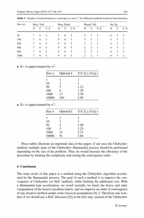
J Optim Theory Appl (2013) 157:148–167 163
Table 3 Number of total iterations to converge to a root x∗ for different methods tested on four functions
Size (n) Broy. Trid. Broy. Band. Bound. Val. Int. Eq.
N C C–S N C C–S N C C–S N C C–S
50 7 6 4 9 8 5 3 3 2 4 3 2
100 7 6 4 9 8 5 3 3 2 4 3 2
200 7 6 4 9 8 5 2 2 1 4 3 2
500 7 6 4 9 8 5 2 2 1 4 3 2
800 7 6 4 9 8 5 2 2 1 4 3 2
1000 7 6 4 9 8 5 2 2 1 4 3 2
• If c is approximated by n2:
Size n Optimal k E(CSk)/E(dC)
1 1 110 1 150 2 1.12100 4 1.291000 17 2.3910000 103 3.95
• If c is approximated by n3:
Size n Optimal k E(CSk)/E(dC)
1 1 110 1 150 2 1.09100 3 1.251000 15 2.3110000 91 3.84
These tables illustrate an important idea of this paper: if one uses the Chebyshevmethod, multiple steps of the Chebyshev–Shamanskii process should be performeddepending on the size of his problem. Thus, he would increase the efficiency of hisprocedure by limiting the complexity and raising the convergence order.
6 Conclusion
The main result of this paper is a method using the Chebyshev algorithm acceler-ated by the Shamanskii process. The goal of such a method is to improve the con-vergence of Chebyshev (or HoC method), while limiting the additional cost. Witha Shamanskii-type acceleration, we avoid (actually we limit) the heavy and riskycomputation of the inverse Jacobian matrix, and we improve an order of convergenceof any iterative method (under some classical assumptions) by 2. Therefore one won-ders if we should use a HoC direction [20] at the first step, instead of the Chebyshev

164 J Optim Theory Appl (2013) 157:148–167
classical method, and then accelerate it by multiple Shamanskii steps. As a matterof fact, HoC methods share the same advantage as Chebyshev, as they require onlyone inverted matrix. Consequently, the global cost of such methods is not significantlyhigher than Chebyshev (as the dominant term remains 1
3n3 coming from the Choleskydecomposition); whereas the convergence order is better (quartic—or more—insteadof cubic). In other words, their efficiency is better than Chebyshev’s. As demonstratedin this paper, it is theoretically and practically possible to improve a HoC method’sconvergence order from ρ to ρ + 2 by a Shamanskii acceleration. The results pre-sented in this paper are concerned with the asymptotic behavior of the Chebyshev–Shamanskii method. We presented details for symmetric systems using the Choleskyfactorization, and such an analysis for general systems using the PLU factorizationis given in Appendix B. The adaptation of our analysis to higher-order methods orother factorizations is straightforward. An important future work concerning suchhigh-order algorithms is the development of a robust and efficient globalization strat-egy for the symmetric case.
Acknowledgements This research was partially supported by NSERC grant OGP0005491, by the Insti-tut des sciences mathématiques (ISM), and the Department of Mathematics of the University of Sherbrooke
Appendix A: Test Functions
We tested our algorithms on the following functions, from the Moré, Garbow andHillstrom collection [1]:
f (x) =m∑
i=1
f 2i (x), (A.1)
where f1, . . . , fm are defined by the following problems. We adopt the followinggeneral format described in [1] and add the expression of Fi = ∂f (x)
∂xi.
Name of function
(a) Dimensions(b) Function definition(c) Standard starting point(d) Minima(e) Expression of the Gradient Fi = ∂f (x)
∂xi.
Thus, our four test functions are:
Problem 1 Broyden tridiagonal function
(a) n variable, m = n
(b) fi(x) = (3 − 2xi)xi − xi−1 − 2xi+1 + 1 where x0 = xn+1 = 0(c) x0 = (−1, . . . ,−1)
(d) f = 0(e) Fi = −4fi−1(x) + 2(3 − 12xi)fi(x) − 2fi+1(x).

J Optim Theory Appl (2013) 157:148–167 165
Table 4 Detailed intrinsic cost for the test functions, considering Eq. (A.1)
Function #(algebraic operations) in Fi = ∂f (x)∂xi
Cost (F = ∇f )
Broyden tridiagonal 5 (+), 10 (–), 16 (*) O(n)
Broyden banded 14 (+), 2 (–), 14 (*) O(n)
Discrete boundary value 4 (+), 2 (–), 12 (*) O(n)
Discrete integral equation (2n + 4) (+), (1 + n/2) (–), (4n + 6) (*) O(n2)
Problem 2 Broyden banded function
(a) n variable, m = n
(b) fi(x) = xi(2 + 5x2i ) + 1 − ∑
j∈Jixj (1 + xi) where Ji = {j : j = i,
max(1, i − ml) ≤ j ≤ min(n, i + mu)} and ml = 5, mu = 1
(c) x0 = (−1, . . . ,−1)
(d) f = 0
(e) Fi = 2(1 + 15x2i − 2xi)fi(x).
Problem 3 Discrete boundary value function
(a) n variable, m = n
(b) fi(x) = 2xi − xi−1 − xi+1 + h2(xi + ti + 1)3/2 where h = 1/n + 1 = 0, ti = ih
and x0 = xn+1 = 0
(c) x0 = (ζj ) where ζj = tj (tj − 1)
(d) f = 0
(e) Fi = −2fi−1(x) + 2[2 + 32h2(xi + ti + 1)2]fi(x) − 2fi+1(x).
Problem 4 Discrete integral equation function
(a) n variable, m = n
(b) fi(x) = xi + h[(1 − ti )∑i
j=1 tj (xj + tj + 1)3 + ti∑n
j=i+1(1 − tj )(xj +tj + 1)3]/2 where h = 1/(n + 1), ti = ih and x0 = xn+1 = 0
(c) x0 = (ζj ) where ζj = tj (tj − 1)
(d) f = 0
(e) Fi = 2[1 + 32hti(xi + ti + 1)2]fi(x).
Table 4 gives details about the costs of the tested problems.
Appendix B: Unsymmetric Systems
If one considers unsymmetric systems, the detailed analysis for the costs involved inhigh-order methods is given in Table 5.
166 J Optim Theory Appl (2013) 157:148–167
Table 5 Costs of operationsinvolved in high-order methodsfor unsymmetric systems
Operation Cost
PLU factorization [21] 23 n3 − 1
2 n2 − 16 n
Solving linear system 2n2 − n
Cost of F c
Obtaining derivative ∇F(xk) with AD [9] nc
∇F(xk)u = ∇(F (xk)u) where u ∈ Rn [25] 5c + 5n
∇2F(xk)uv = ∇(∇(F (xk)u)v) where u,v ∈ Rn 25c + 30n
Vector subtraction or sum n
Thus, the costs of the Newton and Chebyshev methods are:
C(dN) = 2
3n3 + 1
2n2 − 1
6n + (n + 1)c;
C(dC) = 2
3n3 + 5
2n2 + 185
6n + (n + 26)c.
Consequently, the efficiency of the Newton method is
E(dN) = log(2)
23n3 + 1
2n2 − 16n + (n + 1)c
,
and the efficiency of the Chebyshev method is
E(dC) = log(3)
23n3 + 5
2n2 + 1856 n + (n + 26)c
.
As in Sect. 5, we obtain the same ratio between efficiencies of the Chebyshev–Shamanskii method and the Chebyshev method, as the additional cost of theChebyshev–Shamanskii method given in Corollary 3.1 is still valid, i.e.
E(CS)/E(dC) = log(5)
log(3)
cost(dC)
cost(CS)
= log(5)
log(3)
cost(dC)
cost(dC) + 4n2 + 26c + 30n.
Thus, if c is approximated by n2, E(CS)/E(dC) > 1 for n > 22; in other words,the Chebyshev–Shamanskii method is more efficient than the pure Chebyshev’s forn > 22. If c is approximated by n3, then the same result is valid for n > 29.
References
1. Moré, J.J., Garbow, B.S., Hillstrom, K.E.: Testing unconstrained optimization software. ACM Trans.Math. Softw. 7(1), 17–41 (1981)
2. Rall, L.B., Tapia, R.A.: The Kantorovich theorem and error estimates for Newton’s method. Mathe-matics Research (1970)

J Optim Theory Appl (2013) 157:148–167 167
3. Chebyshev, P.L.: Collected works. Number 5. Moscow–Leningrad (1951)4. Halley, E.: A new, exact and easy method of finding roots of any equations generally, and that without
any previous reduction. Philos. Trans. Roy. Soc. (1964)5. Gutiérrez, J.M., Hernández, M.A.: An acceleration of Newton’s method: Super-Halley method. Appl.
Math. Comput. 117(2–3), 223–239 (2001)6. Ezquerro, J.A.: A modification of the Chebyshev method. IMA J. Numer. Anal. 17, 511–525 (1997)7. Ezquerro, J.A., Hernández, M.A.: An improvement of the region of accessibility of Chebyshev’s
method from newton’s method. Math. Comput. 78(264), 1613–1627 (2009)8. Ezquerro, J.A., Hernández, M.A., Romero, N.: On some one-point hybrid iterative methods. Nonlinear
Anal. 72, 587–601 (2010)9. Griewank, A.: Evaluating Derivatives, Principles and Techniques of Algorithmic Differentiation.
SIAM, Philadelphia (2008)10. Zhang, H.: On the Halley class of methods for unconstrained optimization problems. Optim. Methods
Softw. 25(5), 753–762 (2009)11. Shamanskii, V.: On a modification of the Newton method. Mat. Zametki 19, 133–138 (1967)12. Ortega, J.T., Rheinboldt, W.C.: Iterative Solution of Nonlinear Equations in Several Variables. Aca-
demic Press, New York (1970)13. Traub, J.F.: Iterative Methods for the Solution of Equations. Prentice-Hall, Englewood Cliffs (1964)14. Kelley, C.T.: Iterative Methods for Optimization. SIAM, Philadelphia (1995)15. Lampariello, F., Sciandrone, M.: Global convergence technique for the Newton method with periodic
Hessian evaluation. J. Optim. Theory Appl. 111(2), 341–358 (2001)16. Brent, R.P.: Some efficient algorithms for solving systems of nonlinear equations. J. Nucleic Acids
10(2), 327–344 (1973)17. Ostrowski, A.M.: Solutions of Equations in Euclidean and Banach Spaces. Academic Press, New
York (1973)18. Ezquerro, J., Grau-Sánchez, M., Grau, A., Hernández, M., Noguera, M., Romero, N.: On iterative
methods with accelerated convergence for solving systems of nonlinear equations. J. Optim. TheoryAppl. 151(1), 163–174 (2011)
19. Gundersen, G., Steihaug, T.: On large scale unconstrained optimization problems and higher-ordermethods. Optim. Methods Softw. 25(3), 337–358 (2010)
20. Kchouk, B., Dussault, J.-P.: A new family of high order directions for unconstrained optimiza-tion inspired by Chebyshev and Shamanskii methods. Technical report, University of Sherbrooke,Optimization-online.org (2011)
21. Fox, L.: An Introduction to Numerical Linear Algebra. Clarendon Press, Oxford (1964)22. Dussault, J.-P.: High-order Newton-penalty algorithms. J. Comput. Appl. Math. 182(1), 117–133
(2005)23. Baur, W., Strassen, V.: The complexity of partial derivatives. Theor. Comput. Sci. 22, 300–317 (1983)24. Griewank, A.: On automatic differentiation. Math. Program., Recent. Dev. Appl. 6, 83–108 (1989)25. Dussault, J.-P., Hamelin, B., Kchouk, B.: Implementation issues for high-order algorithms. Acta Math.
Vietnam. 34(1), 91–103 (2009)


![A Numerical Comparison of Chebyshev Methods for Solving ...kodu.ut.ee/~benson/ChebyshevArticle10.pdf · review by Luskin [38]. An objective of this study is to show that Chebyshev](https://img.pdfslide.us/doc/110x75/5fa60c71ba6a6171d06ffc2a/a-numerical-comparison-of-chebyshev-methods-for-solving-koduuteebenson-.jpg)