Embed Size (px)
Citation preview

The Chain Ladder Reserve Uncertainties Revisited
by Alois Gisler
Paper to be presented at the ASTIN Colloquium 2016 in Lisbon
Abstract:Chain ladder (CL) is still one of the most popular and most used reserving method for
the insurance practice. In 1993 Mack [7] presented the distribution-free CL-model andderived a formula for the uncertainty of the CL-reserves , which refers to the ultimateprediction uncertainty measured by the mean square error of prediction. For calculatingthe reserve risk and the cost-of-capital loading in solvency (SST and solvency II) one alsoneeds estimators for the one-year prediction uncertainty of all future accounting yearsuntil �nal development.In a recent paper [11] Merz and Wüthrich considered the di¤erent prediction uncer-
tainties, that is the ultimate prediction uncertainty as well as the one year predictionuncertainties for all future accounting years until �nal development within the frame-work of a speci�c Bayesian-CL model. Taking a non-informative prior and after a �rstTaylor approximation they received the already existing result of Mack for the ultimateprediction uncertainty and formulas for the one-year run-o¤ uncertainties for all futureaccounting years until �nal settlement of the run-o¤. However the Bayesian-CL modeland the distribution free CL-model of Mack are two di¤erent pairs of shoes. Thus theresults derived in [11] are results with regard to a di¤erent model and we do not know,whether they are also appropriate in the classical chain ladder model of Mack.In this paper we derive the di¤erent kinds of prediction uncertainties strictly within the
framework of the distribution-free CL model of Mack. By doing so, we gain more insightinto the di¤erences between the two model approaches and �nd the following main results:a) the formulas for the one-year prediction uncertainty in the classical Mack-model aredi¤erent to the Merz-Wüthrich formulas, b) the Merz-Wüthrich formulas are obtained bya �rst order Taylor expansion, c) the Mack formula as well as the Merz-Wüthrich formulasfor the total over all accident years can be written in a simpler way, d) we can see "behindthe formulas", as they can be interpreted in an intuitive and understandable way.
Keywords: claims reserving, distribution free chain-ladder model, Bayesian chain-laddermodel, conditional mean square error of prediction, ultimate run-o¤ uncertainty, one-yearrun-o¤ uncertainties, Mack�s formula, Wuethrich-Merz formulas , cost of capital loading,market value margin.
1

1 Introduction
Accurate claims reserves are essential for an insurance company. It is by far the mostimportant item on the liability side of the balance sheet and has a big impact on thepro�t and loss (P&C) account. A change of the reserves by a small percentage might wellturn a positive year result into a negative one and vice versa. When non-life insurancecompanies went bankrupt, insu¢ cient reserves were mostly one of the main reasons.Chain Ladder (CL) and Bornhuetter Ferguson (BF) are still the most used and most
popular reserving methods in the insurance practice. In this paper we concentrate on theCL-method.CL has been used for decades for calculating reserves. In its origin it is a pure pragmatic
method without an underlying mathematical model. As long as one is only interested inthe reserve estimate, there is no need for a mathematical model. But as soon as one is alsointerested in the accuracy of the CL-reserves, one needs an underlying stochastic model.Under run-o¤ risk we understand the risk of an adverse claims development. It can
be de�ned as minus the claims development result (CDR). As common in the actuarialliterature (see for instance [9]), we will take the conditional mean square error of prediction(msep) as a measure of the reserve uncertainties. For best estimate reserves this msep isequal to the conditional expectation of the square of the CDR. Thereby we distinguishbetween the ultimate run-o¤ risk referring to the ultimate claims development result(CDR) and the one-year run-o¤ risks referring to the CDR resulting in one accountingyear.It was only in 1993 when Mack [7] presented a stochastic CL model and derived a
formula for estimating the msep of the ultimate run-o¤ risk (see Theorem A.1 in appendixA).With the emergence of the new solvency regulation (Swiss solvency test and solvency
II), there arose the need to assess another kind of reserve risk. The risk considered isthe change of risk bearing capital within the next year (one-year time horizon). Hencethe reserve risk relevant for solvency purposes is the one-year run-o¤ risk in the nextaccounting year instead of the ultimate run-o¤ risk considered in Mack. This risk isre�ected under the position "claims development result" or "loss experience previousyears" in next year�s P&L account. A formula for estimating this one year uncertaintyof the next accounting year was �rst published in a paper by Merz and Wüthrich [10] in2008.As the new solvency regulations are based on a market consistent valuation, the best
estimate reserves have to be complemented by a market value margin corresponding tothe discounted costs of capital needed for the entire run-o¤. For this purpose one alsoneeds estimators of the uncertainty of the one-year run-o¤ risk in later accounting yearsuntil the end of the claims development.In a recent paper [11] of end 2014 Merz and Wüthrich reconsidered all the di¤erent
CL reserve uncertainties within a speci�c Bayesian CL model (with Gamma-priors for theCL factors and with conditionally Gamma distributed observations (observed individualCL-factors)), which is very similar to a model which was earlier considered in [4]. Inthis model they derived formulas for all the di¤erent kind of CL-uncertainties inclusivethe one-year run-o¤ uncertainties in future accounting years. For the distribution-freecase, the authors derive the formulas for the reserve uncertainties obtained by taking a
2

non-informative prior followed by a �rst order Taylor approximation. These formulas canbe found in appendix A.However the Bayesian CL-model is di¤erent to the distribution free CL model of Mack.
Thus we do not know whether the results derived in [11] are also appropriate for theclassical Mack model. For instance, in the model considered in [11], the mean square errorof prediction (msep) does only exist, if the observed triangle ful�ls certain properties (seeTheorem 3.8 and condition (4.3) in [11]). But in the Mack-model the msep does alwaysexist.In this paper we derive the di¤erent kinds of prediction uncertainties strictly within the
framework of the distribution-free CL model of Mack. By doing so, we gain more insightinto the di¤erences between the two model approaches and �nd the following main results:
a) The formulas derived for the one-year prediction uncertainty in the classical Mack-model are di¤erent to the Merz-Wüthrich formulas.
b) The Merz-Wüthrich formulas are obtained by a �rst order Taylor expansion.
c) The Mack formula as well as the Merz-Wüthrich formulas for the total over allaccident years can be written in a much simpler way.
d) We can see "behind the formulas", as they can be interpreted in an intuitive andunderstandable way.
e) The derivation of the formulas is straightforward. The mathematics is simple andeasy to understand and makes use of two basic tools, the telescope formula 3.5 andthe estimation principle 3.6.
In this connection it is also worthwhile to remember a discussion in 2006 with regardto the estimation error in the Mack formula. In [2] the authors suggested a di¤erentestimator, which we call the BBMW estimator. There was quite some discussion aboutthese estimators (see [2], [8], [4]). Reconsidering this discussion we come to the conclusionthat the Mack formula for the estimation error is the appropriate one, whereas the BBMWestimator is the adequate formula in the CL-Bayes model, but not in the Mack-model.More details about this side result of the paper can be found in appendix BAt this point we should also mention the most recent paper [12] of Ancus Röhr. He
starts with a �rst order Taylor approximation of the claims development result (CDR)and calculates the prediction uncertainty of this modi�ed CDR. He then also obtains theMack as well as the Merz-Wüthrich results.
Organisation of the paper: In section 2 we introduce some notation and the datastructure. In section 3 we review the CL-reserving method and the stochastic CL-modelof Mack. At the end of this section the telescope formula and the estimation principle arepresented. In section 4 we derive the formula for the ultimate run-o¤ uncertainty (Mack-formula). In section 5 we consider the run-o¤ uncertainty of the next accounting year,whereas in section 6 the formulas for the one-year uncertainties for all future accountingyears until �nal claims development are derived. These results can be compared with theWüthrich-Merz formulas. Finally, a numerical example is presented in section 7.
3

2 Notation and Data Structure
The starting point of claims reserving are observations DI from accident periods i =i0; : : : ; I and development periods j = j0; : : : ; J arranged in a table with i on the verticalaxes and j on the horizontal axes. In the following we will call DI a data triangle, also inthe case, where the shape is a trapezoid.The data in the triangle are denoted by Ci;j > 0 and represent the cumulative claim
�gures (usually claim payments or incurred losses) of accident year i 2 fi0; : : : ; Ig at theend of development year j 2 fj0; : : : ; J): We further assume that the number of accidentyears is bigger or equal to the number of development years, that is J � j0 > I � i0.The index j0 is introduced because in the actuarial literature the �rst development yearis sometimes denoted by zero and sometimes by 1, hence j0 is either zero or one.
j0 j0+1 … j … J
i0
i0+1
…
i
……
I
devolopment years
acci
dent
yea
rs
claims development triangle
At time I; the data Ci;j 2 DI in the upper left part are known, whereas the dataCi;j 2 DcI in the lower right part are future observations we want to predict: We assumethat all claims are settled after development year J and that therefore Ci;J denotes theultimate claim of accident year i.
Some notations:
- diagonal functionsTo simplify notation and as already done by Ancus Röhr in [12] it is convenient tointroduce the diagonal functions
De�nition 2.1 diagonal functions
ji := maxfj such that Ci;j 2 DIg; (1)
ij := maxfi such that Ci;j 2 DIg: (2)
Note that Ci;ji is the diagonal element in row i and that Cij ;j is the diagonal elementin column j.
- The set of observations at time I is given by
DI = fCi;j : i = i0; : : : ; I; j � jig:
4
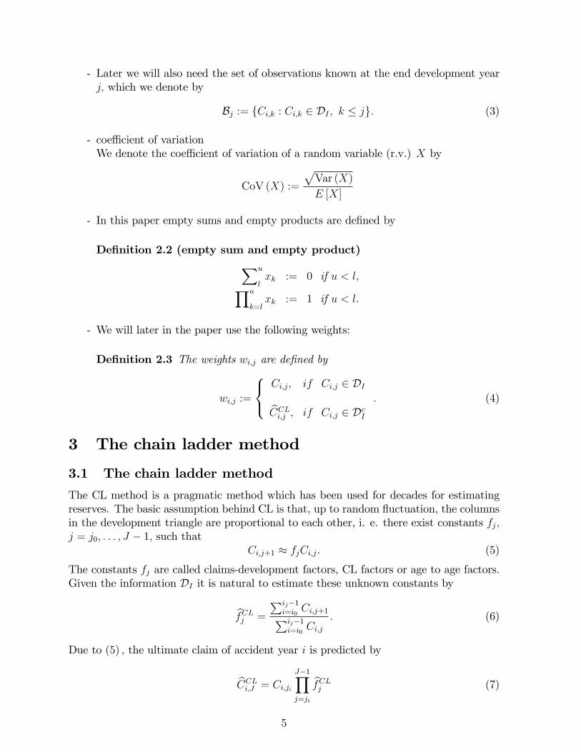
- Later we will also need the set of observations known at the end development yearj; which we denote by
Bj := fCi;k : Ci;k 2 DI ; k � jg: (3)
- coe¢ cient of variationWe denote the coe¢ cient of variation of a random variable (r.v.) X by
CoV (X) :=
pVar (X)
E [X]
- In this paper empty sums and empty products are de�ned by
De�nition 2.2 (empty sum and empty product)Xu
lxk := 0 if u < l;Yu
k=lxk := 1 if u < l:
- We will later in the paper use the following weights:
De�nition 2.3 The weights wi;j are de�ned by
wi;j :=
8<:Ci;j; if Ci;j 2 DI
bCCLi;j ; if Ci;j 2 DcI: (4)
3 The chain ladder method
3.1 The chain ladder method
The CL method is a pragmatic method which has been used for decades for estimatingreserves. The basic assumption behind CL is that, up to random �uctuation, the columnsin the development triangle are proportional to each other, i. e. there exist constants fj;j = j0; : : : ; J � 1; such that
Ci;j+1 � fjCi;j. (5)
The constants fj are called claims-development factors, CL factors or age to age factors.Given the information DI it is natural to estimate these unknown constants by
bfCLj =
Pij�1i=i0
Ci;j+1Pij�1i=i0
Ci;j: (6)
Due to (5) ; the ultimate claim of accident year i is predicted by
bCCLi;J = Ci;ji J�1Yj=ji
bfCLj (7)
5

and the Ci;j in the lower right part of the triangle are estimated by
bCCLi;j = Ci;ji j�1Yk=ji
bfCLk for i = i0; : : : ; I; j = ji + 1; : : : ; J: (8)
(8) are called the CL-predictions. It is also useful and meaningful to de�nebCCLi;j := Ci;j for Ci;j 2 DI : (9)
The CL reserve bRCLi of accident year i is an estimate of the outstanding liabilities
Ri =JX
j=ji+1
Ci;j (10)
and is the di¤erence between the CL prediction bCCLi;J of the ultimate claim and the cumu-lative claim Ci;ji known at time I; i.e.bRCLi = bCCLi;J � Ci;ji (11)
Finally bRCLtot = IXi=i0
bRCLi (12)
is the total reserve over all accident years.
3.2 The stochastic CL-model of Mack
The following distribution-free stochastic model underlying the CLmethod was introducedin [7] by Mack .
Model Assumptions 3.1 (Mack-model)
i) Cumulative claims Ci;j of di¤erent accident years are independent.
ii) There exist positive parameters fj0 ; : : : ; fJ�1 and �2j0; : : : ; �2J�1 such that for all i =
i0; : : : ; I; and all j = j0; : : : ; J � 1
E[Ci;j+1jCi;j0 ; Ci;j0+1; : : : ; Ci;j] = fjCi;j; (13)
Var(Ci;j+1jCi;j0 ; Ci;j0+1; : : : ; Ci;j) = �2jCi;j (14)
It is useful to introduce the individual CL ratios
Fi;j :=Ci;j+1Ci;j
: (15)
Because of model assumptions 3.1 Fi;j belonging to di¤erent accident years are indepen-dent and it holds that
E[Fi;jjBj] = fj; (16)
Var(Fi;jjBj) =�2jwi;j
with wi;j = Ci;j: (17)
6
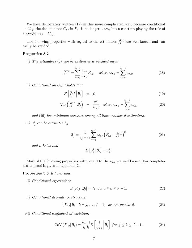
We have deliberately written (17) in this more complicated way, because conditionalon Ci;j; the denominator Ci;j in Fi;j is no longer a r.v., but a constant playing the role ofa weight wi;j = Ci;j:
The following properties with regard to the estimators bfCLj are well known and caneasily be veri�ed:
Properties 3.2
i) The estimators (6) can be written as a weighted mean
bfCLj =
ij�1Xi=i0
wi;jw�;j
Fi;j; where w�;j =ij�1Xi=i0
wi;j; (18)
ii) Conditional on Bj; it holds that
Eh bfCLj ���Bji = fj; (19)
Var� bfCLj ���Bj� =
�2jw�;j
, where w�;j =ij�1Xi=i0
wi;j; (20)
and (19) has minimum variance among all linear unbiased estimators.
iii) �2j can be estimated by
b�2j = 1
ij � i0
ij�1Xi=i0
wi;j
�Fi;j � bfCLj �2
(21)
and it holds thatE�b�2j ��Bj� = �2j :
Most of the following properties with regard to the Fi;j are well known. For complete-ness a proof is given in appendix C.
Properties 3.3 It holds that
i) Conditional expectation:
E [Fi;kj Bj] = fk for j � k � J � 1; (22)
ii) Conditional dependence structure:
fFi;kj Bj : k = j; : : : ; J � 1g are uncorrelated, (23)
iii) Conditional coe¢ cient of variation:
CoV (Fi;kj Bj) =�kfk
sE
�1
Ci;k
����Bj� for j � k � J � 1: (24)
7

3.3 Mean square error of prediction, telescope formula and es-timation principle
As measure for the CL reserve uncertainty we use the conditional mean square error ofprediction (msep).
De�nition 3.4 The conditional mean square error of prediction (msep) of the CL pre-diction bCCLi;J is de�ned by
msepCi;J jDI� bCCLi;J � := E �� bCCLi;J � Ci;J�2����DI�
The conditional msep of other predictors and estimators are analogously de�ned. Notethat
msepRijDI
� bRCLi � = msepCi;J jDI � bCCLi;J � ;since bRCLi = bCCLi;J � Ci;ji and since Ci;ji is known at time I.To derive estimators of this msep we will make extensive use of the following telescope
formula.
Lemma 3.5 (Telescope Formula) For any real numbers xj and yj; j = 1; 2; : : : ; J , itholds that YJ
j=1xi �
YJ
j=1yi =
JXj=1
j�1Yk=1
xk
!(xj � yj)
IY
m=i+1
ym
!: (25)
Proof:This result is well known. We show it for a product with J = 3: The extension to anynumber J is self evident.
x1x2x3 � y1y2y3 = x1x2x3 � x1x2y3 + x1x2y3 � x1y2y3 + x1y2y3 � y1y2y3= (x1 � y1) y2y3 + x1 (x2 � y2) y3 + x1x2 (x3 � y3) :
2
In the formulas of the conditional msep there appear the unknown CL factors fj: To �ndan estimator for the msep we have to estimate these unknown constants. As a generalprinciple we replace them by the estimators bfj: But we can�t do it for the quadraticdi¤erence terms
� bfCLj � fj�2; because this would give an estimator of zero, which is not
meaningful. To �nd an estimator we have to study the �uctuation of bfCLj around fj: Forthis purpose we take into account as many observations of DI as possible and considerthe conditional r.v. bfCLj ���Bj with moments
Eh bfCLj ���Bji = fj; (26)
E
�� bfCLj � fj�2����Bj� =
�2jPij�1i=i0
wi;j: (27)
Based on (27) we will use the following estimation principle:
8
Estimation Principle 3.6
a)
estimator of� bfCLj � fj
�2:= bE �(Fj � fj)2��Bj� = b�2jPij�1
i=i0wi;j
: (28)
b) Other functions of fj such asQJj=ji
f 2j are estimated by replacing the unknown fjby bfCLj :
Remarks:
- Note that
�2jf 2j
1Pij�1i=i0
wi;j=
�CoV
� bfCLj ���Bj��2 and hence
b�2jbfCLj 1Pij�1i=i0
wi;j=
�dCoV � bfCLj ���Bj��2 : (29)
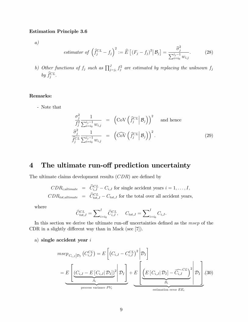
4 The ultimate run-o¤ prediction uncertainty
The ultimate claims development results (CDR) are de�ned by
CDRi;ultimate = bCCLi;J � Ci;J for single accident years i = 1; : : : ; I;CDRtot;ultimate = bCCLtot;J � Ctot;J for the total over all accident years,
where bCCLtot;J =XI
i=i0
bCCLi;J ; Ctot;J =XI
i=i0Ci;J :
In this section we derive the ultimate run-o¤ uncertainties de�ned as the msep of theCDR in a slightly di¤erent way than in Mack (see [7]).
a) single accident year i
msepCi;J jDI�CCLi;J
�= E
��Ci;J � CCLi;J
�2 ����DI�
= E
24(Ci;J � E [Ci;J j DI ])| {z }Ai
2
������DI35
| {z }process variance PVi
+ E
2664�E [Ci;J j DI ]�dCi;JCL�| {z }Bi
2
��������DI3775
| {z }estimation error EEi
:(30)
9

Process Variance PVi :
Ai = Ci;ji
J�1Yj=ji
Fi;j �J�1Yj=ji
fj
!;
where the diagonal element Ci;ji is a multiplicative constant playing the role of aweight wi;ji :
By applying the telescope formula (25) we obtain
Ai = wi;ji
((Fi;ji � fji)
J�1Yj=ji+1
fj + : : :+
j�1Yk=ji
Fi;j (Fi;j � fj)J�1Yl=k+1
fl
: : : +
J�2Yk=ji
Fi;k (Fi;J�1 � fJ�1)):
=J�1Xj=ji
Ci;j (Fi;j � fj)J�1Yk=j+1
fk:
Hence
PVi = E�A2i��DI� = E
24 J�1Xj=ji
�Ci;j (Fi;j � fj)
YJ�1
k=j+1fk
�!2DI
35 : (31)
The cross terms vanish since
E [Ci;jCi;j+k (Fi;j � fj) (Fi;j+k � fj+k)j DI ] == E [E [Ci;jCi;j+k (Fi;j � fj) (Fi;j+k � fj+k)j Bj+k]j DI ] = 0 for k > 0;(32)
where we have used that fFi;j+k : k > 0g are conditionally unbiased given Bj+k:Hence
PVi =J�1Xj=ji
E
�Ci;j (Fi;j � fj)2
�YJ�1
k=j+1fk
�2����DI�
=J�1Xj=ji
E
24E24 Ci;j (Fi;j � fj) J�1Y
k=j+1
fk
!2������Bj35DI
35=
J�1Xj=ji
E [Ci;jj DI ]
J�1Yk=j+1
f 2k
!�2j (33)
=J�1Xj=ji
E [Ci;J j DI ]2�2jf 2j
1
E [Ci;jj DI ]: (34)
By applying the estimation principle 3.6 we obtain
dPV i = � bCCLi;J �20B@J�1Xj=ji
b�2j� bfCLj �2 1
wi;j
1CA ; (35)
10
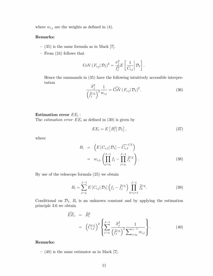
where wi;j are the weights as de�ned in (4).
Remarks:
� (35) is the same formula as in Mack [7].
�From (24) follows that
CoV (Fi;jj DI)2 =�2jf 2jE
�1
Ci;j
����DI� :Hence the summands in (35) have the following intuitively accessible interpre-tation b�2j� bfCLj �2 1
wi;j= dCoV (Fi;jj DI)2 : (36)
Estimation error EEi :The estimation error EEi as de�ned in (30) is given by
EEi = E�B2i��DI� ; (37)
where
Bi =�E [Ci;J j DI ]�dCi;JCL�
= wi;ji
J�1Yj=ji
fj �J�1Yj=ji
bfCLj!: (38)
By use of the telescope formula (25) we obtain
Bi =J�1Xj=ji
E [Ci;jj DI ]�fj � bfCLj � J�1Y
k=j+1
bfCLk : (39)
Conditional on DI ; Bi is an unknown constant and by applying the estimationprinciple 3.6 we obtain
dEEi = bB2i=
� bCCLi;J �28><>:J�1Xj=ji
b�2j� bfCLj �2 1Xij�1
i=i0wi;j
9>=>; : (40)
Remarks:
� (40) is the same estimator as in Mack [7].
11

� In (41) we have seen hat
b�2j� bfCLj �2 1Xij�1
i=i0wi;j
= dCoV � bfCLj ���Bj�2 ; (41)
which is an intuitively accessible interpretation of the summands in (40) :
b) Total over all accident years
Process Variance PVtotSince di¤erent accident years are independent it follows that
dPV tot =IX
i=i0
dPV i = IXi=iJ+1
dPV i=
IXi=iJ+1
� bCCLi;J �20B@J�1Xj=ji
b�2j� bfCLj �2 1
wi;j
1CA :By changing the order of summation between i and j we obtain
dPV tot = J�1Xj=j0
b�2j� bfCLj �2 IXi=ij
1
wi;j
� bCCLi;J �2 : (42)
Estimation Error EEtot
EEtot = E�B2tot
��DI� ;where
Btot =IX
i=i0
Bi =IX
i=iJ+1
Bi
=IX
i=iJ+1
J�1Xj=ji
E [Ci;jj DI ]J�1Yk=j+1
bfCLk!:
Changing the order of summation between i and j yields
Btot =J�1Xj=j0
0@ IXi=ij
E [Ci;jj DI ]J�1Yk=j+1
bfCLk1A�fj � bfCLj �
:
By by applying the estimation principle 3.6 we �nd
dEEtot = J�1Xj=i0
b�2j� bfCLj �2�PI
i=ijbCCLi;J �2�Pi=ij�1
i=i0wi;j
� : (43)
12

Remarks:
�Note that
dEEtot > IXi=0
dEEi = J�1Xj=i0
b�2j� bfCLj �2PI
i=ij
� bCCLi;J �2�Pi=ij�1i=i0
wi;j
� :c) resultThe results in the following Theorem except formula (46) are a summary of (30) ; (35) ;(40) ; (42) ; (43) :
Theorem 4.1 The msep of the ultimate run-o¤ risk can be estimated by
a) single accident year i
[msepCi;J jDI� bCCLi;J � = � bCCLi;J �2
8><>:J�1Xj=ji
b�2j� bfCLj �2 1
wi;j+
1Pij�1i=i0
wi;j
!9>=>; (44)
where the weights wi;j are de�ned in (4) ;
b) total over all accident years
[msepCtot;J jDI� bCCLtot;J� = J�1X
j=j0
8><>: b�2j� bfCLj �20B@ IXi=ij
� bCCLi;J �2wi;j
+
�PIi=ij
bCCLi;J �2Pij�1i=i0
wi;j
1CA9>=>;(45)
=� bCCLtot;J�2
PIi=ij
bCCLi;JbCCLtot;J! b�2j� bfCLj �2 1Pij�1
i=i0wi;j
; (46)
where bCCLtot;J =XI
i=i0
bCCLi;J :Remarks:
�The �rst summand in (44) and (45) represent the process variance and thesecond one the estimation error.
� (44) is the same formula as the Mack formula (95) in appendix A. However,(45) and (46) look di¤erent to the Mack formula (96) in appendix A. Thecovariance terms have disappeared, they are much simpler and have an intu-itively understandable interpretation (see the second last bullet point of theseremarks). But they give the same results as (96) :
�Formula (46) was already found by Ancus Röhr in [12]. But his derivation is lessstringent, as he did not calculate the msep of the ultimate claims developmentresult CDRult; but the msep of CDRult, where CDRult is a �rst order Taylorexpansion of CDRult.
13

�For the process error the uncertainties due to the Fi;j sum up, whereas forthe estimation error several accident years are a¤ected simultaneously by theuncertainty of bfCLj . This is the reason why
dPV tot = IXi=i0
dPV i; butdEEtot > IXi=i0
dEEi:�intuitively accessible interpretationFrom (36) and (29) we see that (44) and (45) can be written as
[msepCi;J jDI� bCCLi;J � = � bCCLi;J �2
(J�1Xj=ji
�dCoV (Fi;jj Bj)2 + dCoV � bfCLj ���Bj�2�) ;(47)
[msepCtot;J jDI� bCCLtot;J� =
� bCCLtot;J�2�XJ�1
j=j0qj
�dCoV � bfCLj ���Bj��2� ; (48)
where qj =
PIi=ij
bCCLi;JbCCLtot;J is the fraction of bCCLtot;J , which is a¤ectedby the uncertainty of bfCLj : (49)
(47) and (48) give a good intuitive understanding of (44) and (46) ; as the
coe¢ cients of variation CoV (Fi;jj Bj) and CoV� bfCLj ���Bj� are good intuitive
measures for the relative deviation of Fi;j and bfCLj from the "true" CL-factorsfj: In particular, (48) is a very intuitive formula.
� Instead of distinguishing between the process variance and the estimation errorwe could apply the telescope formula (25) directly to the ultimate run-o¤ risk
Zi;ult = Ci;J � bCCLi;J= wi;ji
J�1Yj=ji
Fi;j �J�1Yj=ji
bfCLj!
= wi;ji
J�1Xj=ji
(j�1Yk=ji
Fi;k
�Fi;j � bfCLj � J�1Y
m=j+1
bfCLm)
=
J�1Xj=ji
Ci;j (Fi;j � fj)J�1Y
m=j+1
bfCLm| {z }Ai
+
J�1Xj=ji
Ci;j
�fj� bfCLj � J�1Y
m=j+1
bfCLm| {z }Bi
:(50)
However the summands in (50) are correlated, such that the calculation ofE�Z2i;ult
��DI� is rather complicated. But note that the Ci;j in Bi play the roleof "stochastic weights", which are not yet known. A natural procedure is to
14

replace them by the forecasted weights wi;j = bCCLi;j and to considereZi;ult = J�1X
j=ji
Ci;j (Fi;j � fj)J�1Y
m=j+1
bfCLm +J�1Xj=ji
wi;j
�fj� bfCLj � J�1Y
m=j+1
bfCLm : (51)
Then we immediately get;
bE h eZ2i;ult���DIi = � bCCLi;J �28><>:J�1Xj=ji
b�2j� bfCLj �2 1
wi;j+
1Pij�1i=i0
wi;j
!9>=>; ;which is the same result as the one found in Theorem 4.1: Hence by replacingthe not yet known stochastic weights in Bi by the forecasted weights wi;j andthen calculating the msep of the modi�ed r.v. eZi;ult we end up with the "cor-rect" estimator (44) :
Proof of Theorem 4.1:It only remains to prove that (45) can be expressed by (46) :
J�1Xj=j0
8><>: b�2j� bfCLj �20B@ IXi=ij
� bCCLi;J �2wi;j
+
�PIi=ij
bCCLi;J �2Pij�1i=i0
wi;j
1CA9>=>; =
=J�1Xj=j0
8><>: b�2j� bfCLj �2 J�1Yk=j
bfCLk!0@0@ IX
i=ij
bCCLi;J1A 1 + PI
i=ijbCCLi;JPij�1
i=i0bCCLi;J
!1A9>=>;
=J�1Xj=j0
8><>: b�2j� bfCLj �2 J�1Yk=j
bfCLk!0@ IX
i=ij
bCCLi;J1A bCCLtot;JPij�1
i=i0bCCLi;J
!9>=>;=
� bCCLtot;J�20B@J�1Xj=j0
b�2j� bfCLj �2 1Pij�1i=i0
wi;j
PIi=ij
bCCLi;JbCCLtot;J1CA :
2
5 The one-year run-o¤ prediction uncertainty of thenext accounting year
In the new solvency regulation (SST, Solvency II), a time horizon of one year is considered.Therefore the reserve risk relevant for solvency purposes is the one-year run-o¤ risk of thenext accounting year.In the previous section, claims reserving was considered from a static perspective. For
solvency purposes, the claims reserving has to be seen as a dynamic process, where the
15
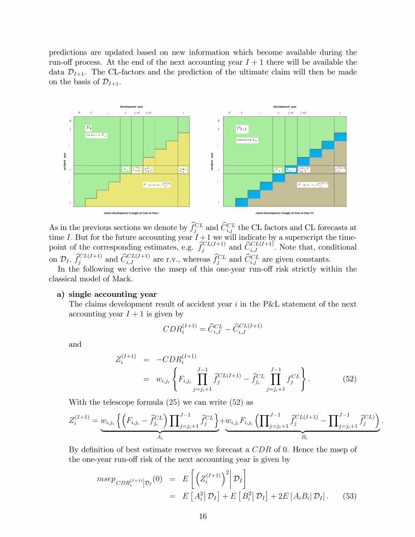
predictions are updated based on new information which become available during therun-o¤ process. At the end of the next accounting year I + 1 there will be available thedata DI+1. The CL-factors and the prediction of the ultimate claim will then be madeon the basis of DI+1:
0 1 j i j i +1 j i +2 J
0
1
….
i
I
acci
dent
yea
r
….
claims development triangle at time at time I
development year
… … 0 1 j i j i +1 j i +2 J
0
1
….
i
I
development year
… …
acci
dent
yea
r
….
claims development triangle at time at time I+1
As in the previous sections we denote by bfCLj and bCCLi;j the CL factors and CL forecasts attime I: But for the future accounting year I+1 we will indicate by a superscript the time-point of the corresponding estimates, e.g. bfCL(I+1)j and bCCL(I+1)i;J : Note that, conditional
on DI ; bfCL(I+1)j and bCCL(I+1)i;J are r.v., whereas bfCLj and bCCLi;j are given constants.In the following we derive the msep of this one-year run-o¤ risk strictly within the
classical model of Mack.
a) single accounting yearThe claims development result of accident year i in the P&L statement of the nextaccounting year I + 1 is given by
CDR(I+1)i = bCCLi;J � bCCL(I+1)i;J
and
Z(I+1)i = �CDR(I+1)i
= wi;ji
(Fi;ji
J�1Yj=ji+1
bfCL(I+1)j � bfCLji J�1Yj=ji+1
fCLj
): (52)
With the telescope formula (25) we can write (52) as
Z(I+1)i = wi;ji
n�Fi;ji � bfCLji �YJ�1
j=ji+1
bfCLj o| {z }
Ai
+wi;jiFi;ji
�YJ�1
j=ji+1
bfCL(I+1)j �YJ�1
j=ji+1
bfCL)j
�| {z } :
Bi
By de�nition of best estimate reserves we forecast a CDR of 0. Hence the msep ofthe one-year run-o¤ risk of the next accounting year is given by
msepCDR
(I+1)i
���DI (0) = E
��Z(I+1)i
�2����DI�= E
�A2i��DI�+ E �B2i ��DI�+ 2E [AiBij DI ] : (53)
16

For the �rst summand in (53) we get
E�A2i��DI� = w2i;ji
�E�(Fi;ji � fji)
2��DI�+ �fji � bfCLji �2�YJ�1
j=ji+1
� bfCLj �2= wi;ji�
2ji
YJ�1
j=ji+1
� bfCLj �2+ w2i;ji
�fji � bfCLji �2YJ�1
j=ji+1
� bfCLj �2;
which, by use of the the estimation principle 3.6, is estimated by
bE �A2i ��DI� = � bCCLi;J �2 b�2ji� bfCLji �28><>: 1
wi;ji+
1Xi�1
k=i0wk;ji
9>=>; : (54)
For estimating the second and the third summand in (53) we �rst note that
bfCL(I+1)j � bfCLj =
Piji=i0
wi;jFi;jPiji=i0
wi;j�Pij�1
i=i0wi;jFi;jPij�1
i=i0wi;j
= aj
�Fij ;j � bfCLj �
; (55)
whereaj =
wij ;jPiji=i0
wi;j: (56)
Since the observations of di¤erent accident years are independent it follows thatnFi;ji ;
bfCL(I+1)ji+1; : : : ; f
CL(I+1)J�1
oare independent, (57)nbfCL(I+1)j0
; bfCL(I+1)j0+1; : : : ; f
CL(I+1)J�1
oare independent. (58)
From the model assumptions 3.1 and from (55) and (57) follows that
E�F 2i;ji
��DI� = f 2ji +�2jiwi;ji
;
Eh bfCL(I+1)j
���DIi = bfCLj + aj
�fj � bfCLj �
;
Var� bfCL(I+1)j
���DI� = a2j�2jiwi;ji
;
E
�� bfCL(I+1)j
�2����DI� =� bfCLj + aj
�fj � bfCLj ��2
+ a2j�2jwi;ji
;
and, by applying the estimation principle 3.6,
bE �F 2i;ji��DI� =� bfCLji �2 + b�2ji
wi;ji(59)
bE h bfCL(I+1)j
���DIi = bfCLj ; (60)
bE �� bfCL(I+1)j
�2����DI� =� bfCLj �2
+ a2jb�2j
1Pij�1i=i0
wi;j+
1
wi;ji
!=
� bfCLj �2+ bjb�2j ; (61)
17
wherebj =
wij ;j�Pij�1i=i0
wi;j
��Piji=i0
wi;j
� : (62)
With the estimation principle 3.6 we immediately obtain thatbE [AiBij DI ] = 0; (63)
since bE h�YJ�1
j=ji+1
bfCL(I+1)j �YJ�1
j=ji+1fCL)j
����DIi = 0:From (57) and (59) follows that the second summand in (53) can be estimated by
bE �B2i ��DI� = w2i;ji( �bfCLji �2 + b�2ji
wi;ji
! J�1Yj=ji+1
��bfCLj �2+ bjb�2j�� J�1Y
j=ji+1
� bfCLj �2!)
= w2i;ji
J�1Yj=ji
� bfCLj �28><>:0B@1 + 1
wi;ji
b�2ji� bfCLji �21CA0B@ J�1Yj=ji+1
0B@1 + bj b�2j� bfCLj �21CA� 1
1CA9>=>; : (64)
By plugging (54) ; (63) ; (64) into (53) we get
bE ��Z(I+1)i
�2����DI� = � bCCLi;J �2 b�2ji� bfCLji �28><>: 1
wi;ji+
1Xi�1
k=i0wk;ji
9>=>;+ (65)
+� bCCLi;J �2
8><>:0B@1 + 1
wi;ji
b�2ji� bfCLji �21CA0B@ J�1Yj=ji+1
0B@1 + bj b�2j� bfCLj �21CA� 1
1CA9>=>; :
Remarks:
�From (60) and (61) we see that
bjb�2j� bfCLj �2 = dCoV � bfCL(I+1)j
���DI�2 ; (66)
which is an intuitively accessible interpretation.
�Note the di¤erence betweendCoV � bfCLji ���Bji� = measure, how much bfCLji will deviate from fj; if only
the data Bji are considered as known and non random
anddCoV � bfCL(I+1)j
���DI� = measure how much bfCL(I+1)j will deviate from bfCLj if
all data DI are considered as known and non random.
18
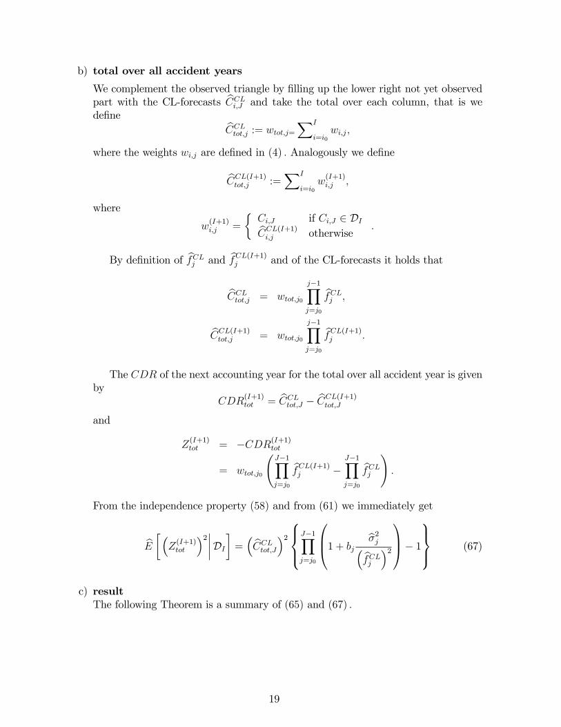
b) total over all accident years
We complement the observed triangle by �lling up the lower right not yet observedpart with the CL-forecasts bCCLi;J and take the total over each column, that is wede�ne bCCLtot;j := wtot;j=XI
i=i0wi;j;
where the weights wi;j are de�ned in (4) : Analogously we de�ne
bCCL(I+1)tot;j :=XI
i=i0w(I+1)i;j ;
where
w(I+1)i;j =
�Ci;J if Ci;J 2 DIbCCL(I+1)i;j otherwise
:
By de�nition of bfCLj and bfCL(I+1)j and of the CL-forecasts it holds that
bCCLtot;j = wtot;j0
j�1Yj=j0
bfCLj ;
bCCL(I+1)tot;j = wtot;j0
j�1Yj=j0
bfCL(I+1)j :
The CDR of the next accounting year for the total over all accident year is givenby
CDR(I+1)tot = bCCLtot;J � bCCL(I+1)tot;J
and
Z(I+1)tot = �CDR(I+1)tot
= wtot;j0
J�1Yj=j0
bfCL(I+1)j �J�1Yj=j0
bfCLj!:
From the independence property (58) and from (61) we immediately get
bE ��Z(I+1)tot
�2����DI� = � bCCLtot;J�28><>:J�1Yj=j0
0B@1 + bj b�2j� bfCLj �21CA� 1
9>=>; (67)
c) resultThe following Theorem is a summary of (65) and (67) :
19

Theorem 5.1 The msep of the one year run-o¤ risk in the next accounting yearI+1 can be estimated by
a) single accident year
[msepCDR
(I+1)i
���DI (0) =� bCCLi;J �2 b�2ji� bfCLji �2
8><>: 1
wi;ji+
1Xi�1
k=i0wk;ji
9>=>;+
+� bCCLi;J �2
8><>:0B@1 + 1
wi;ji
b�2ji� bfCLji �21CA0B@ J�1Yj=ji+1
0B@1 + bj b�2j� bfCLj �21CA� 1
1CA9>=>; ; (68)
where
bj =wij ;j�Pij�1
i=i0wi;j
��Piji=i0
wi;j
� ; (69)
wi;j as de�ned in (4) :
b) total over all accident years
[msepCDR
(I+1)tot
���DI (0) =� bCCLtot;J�2
8><>:J�1Yj=j0
0B@1 + bj b�2j� bfCLj �21CA� 1
9>=>; ; (70)
where bj is given by (69) :
Remarks:
�The �rst summand in (68) re�ects the risk that the observation on the nextdiagonal will deviate from the forecast at time I:
�The second summand in (68) re�ects the risk of updating the forecasts of laterdevelopment years due to an update of the estimated CL-factors from time Ito time I + 1.
�The estimator (70) is surprisingly simple and even simpler than the estimator(71) for a single accident year .
�intuitively accessible interpretationFrom (29), (36) and (66) we see thatb�2ji� bfCLji �2
1
wi;ji= dCoV (Fi;jj Bj)2 ;
b�2ji� bfCLji �21Xi�1
k=i0wk;ji
= dCoV � bfCLj ���Bj�2 ;bj
b�2j� bfCLj �2 = dCoV � bfCLj ���DI�2 ;20
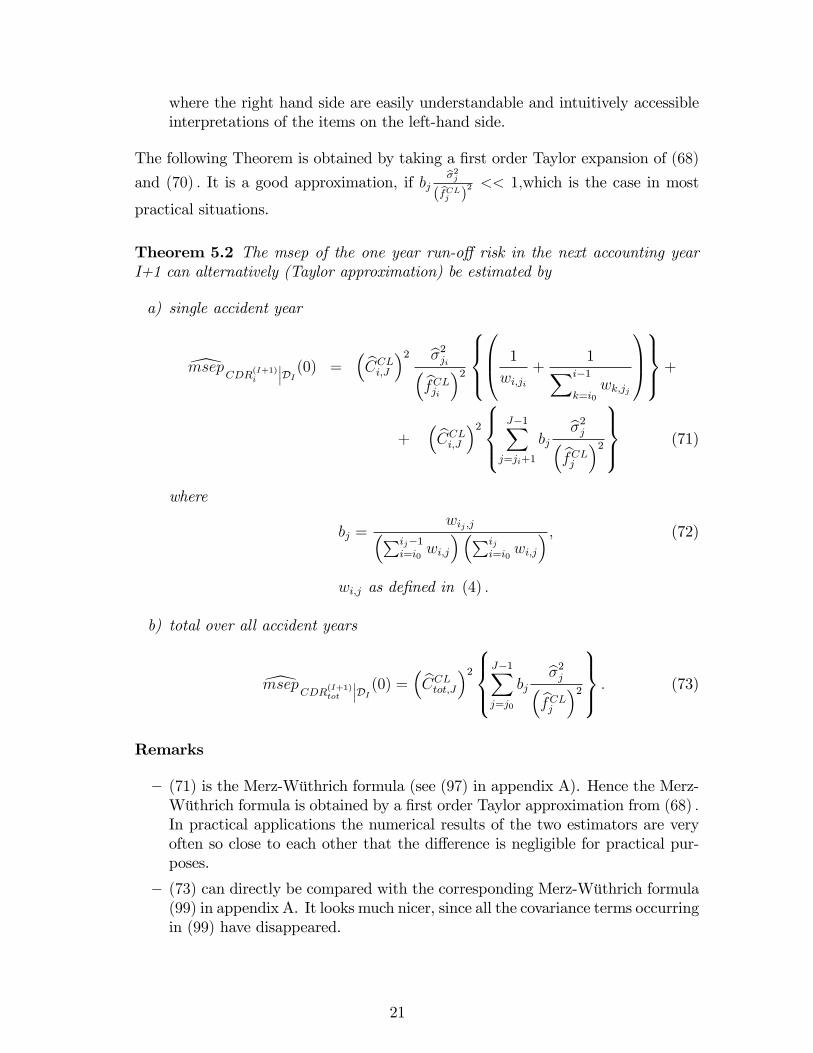
where the right hand side are easily understandable and intuitively accessibleinterpretations of the items on the left-hand side.
The following Theorem is obtained by taking a �rst order Taylor expansion of (68)
and (70) : It is a good approximation, if bjb�2j
( bfCLj )2 << 1;which is the case in most
practical situations.
Theorem 5.2 The msep of the one year run-o¤ risk in the next accounting yearI+1 can alternatively (Taylor approximation) be estimated by
a) single accident year
[msepCDR
(I+1)i
���DI (0) =� bCCLi;J �2 b�2ji� bfCLji �2
8><>:0B@ 1
wi;ji+
1Xi�1
k=i0wk;jj
1CA9>=>;+
+� bCCLi;J �2
8><>:J�1Xj=ji+1
bjb�2j� bfCLj �2
9>=>; (71)
where
bj =wij ;j�Pij�1
i=i0wi;j
��Piji=i0
wi;j
� ; (72)
wi;j as de�ned in (4) :
b) total over all accident years
[msepCDR
(I+1)tot
���DI (0) =� bCCLtot;J�2
8><>:J�1Xj=j0
bjb�2j� bfCLj �2
9>=>; : (73)
Remarks
� (71) is the Merz-Wüthrich formula (see (97) in appendix A). Hence the Merz-Wüthrich formula is obtained by a �rst order Taylor approximation from (68) :In practical applications the numerical results of the two estimators are veryoften so close to each other that the di¤erence is negligible for practical pur-poses.
� (73) can directly be compared with the corresponding Merz-Wüthrich formula(99) in appendix A. It looks much nicer, since all the covariance terms occurringin (99) have disappeared.
21
�intuitively accessible interpretationAnalogously as in Theorem 5.1 we can look behind the formulas and we canwrite (71) and (73) as
[msepCDR
(I+1)i
���DI (0) =� bCCLi;J �2�dCoV (Fi;jij Bji)2 + dCoV � bfCLji ���Bji�2�++� bCCLi;J �2
(J�1Xj=ji+1
dCoV � bfCL(I+1)j
���DI�2) ; (74)[msep
CDR(I+1)tot
���DI (0) =� bCCLtot;J�2
(J�1Xj=j0
dCoV � bfCL(I+1)j
���DI�2) ; (75)
which are intuitively accessible interpretations of (71) and (73) :
6 The one-year run-o¤ prediction uncertainty in fu-ture accounting years
In the SST and in solvency II, the market value margin corresponding to the run-o¤risk equals the discounted cost of capital, which is needed at the end of each accountingyear for the one year run-o¤ risk in the next accounting year. For this purpose we needestimates of the one year run-o¤ risk for the accounting years I + k; k = 1; : : : ; J � 1;evaluated at time I:
6.1 The Compatibility Condition
Note that the one-year CDR in the accounting years I + k; k = 1; : : : ; J are given by
CDR(I+k)i = bCCL(I+k�1)i;J � bCCL(I+k)i;J ;
CDR(I+k)tot = bCCL(I+k�1)tot;J � bCCL(I+1+k)tot;J :
Note also that accident year i is already fully developed in the accounting years fI + k : k � J � jigand that therefore bCCL(I+k)i;J = Ci;J for k � J � ji:The sum of the one year claims development results over all future development years
is equal to the ultimate claims development result. Hence the one-year run-o¤ risksZ(I+k)i = �CDR(I+k)i satisfyXJ�ji
k=1Z(I+k)i = Ci;J � bCCLi;J ; (76)XJ
k=1Z(I+k)tot = Ctot;J � bCCLtot;J ; (77)
and hence
E
��XJ
k=1Z(I+k)i
�2����DI� = E
�� bCCLi;J � Ci;J�2����DI� = msepCi;J jDI � bCCLi;J � ; (78)
E
��XJ
k=1Z(I+k)tot
�2����DI� = E
�� bCCLtot;J � Ci;J�2����DI� = msepCtot;J jDI � bCCLtot;J� :(79)22

By de�nition of best estimate reserves the forecast of the claims development resultin future periods is always zero. For this reason it is often argued that the process ofbest estimate forecasts
n bCBE(I+k)i;J : k = 0; : : : ; Jois a martingale and that therefore the
one-year CDR, which are the increments of this process, are independent. Based on thismartingale argument it is then required that the estimators of the one-year run-o¤ riskshould satisfy the following "splitting" property:
De�nition 6.1 (splitting property) Estimators of the msep of the one year run-o¤risk ful�l the "splitting property" ifXJ
k=1[msep
CDR(I+k)i jDI
(0) = [msepCi;J jDI� bCCLi;J � for i = i0; : : : ; I , (80)XJ
k=1[msep
CDR(I+k)tot jDI
(0) = [msepCtot;J jDI� bCCLtot;J� ; (81)
where the right hand side of (80) and (81) are given by Theorem 4.1.
Remarks:
� The "splitting property" means that the ultimate run-o¤ prediction uncertainty issplit over all future accounting years until �nal development.
However best estimate forecasts are usually not a martingale, which is also the case forthe CL-forecasts. The CL forecasts ful�lbE h bCCL(I+k+1)i;J
��� bCCL(I+k)i;J
i= bCCL(I+k)i;J ;
but they do not satisfy the martingale condition
Eh bCCL(I+k+1)i;J
��� bCCL(I+k)i;J
i= bCCL(I+k)i;J ;
because the unknown CL factors fj are replaced in the CL-forecasts by its estimates bfCLjand bfCL(I+1+k)j respectively.Assume, that the required capital (risk margin) for the run-o¤ risk is calculated by a
�xed percentage of the msep (variance risk measure) and that we consider only nominalcash-�ows (no interest income). The requirement, to have enough capital for the ultimaterun-o¤ risk is a weaker condition than the requirement, that this capital is also su¢ cientto meet, from a today�s perspective, the capital requirement for the one-year run-o¤ riskat the beginning of each future accounting year until �nal claims development. Thereforethe msep for the ultimate run-o¤ risk is a lower bound for the sum of the msep of theone-year run-o¤ risk. For this reason the estimators for the one-year run-o¤ risk shouldsatisfy the following "compatibility" condition:
Condition 6.2 (compatibility) Estimators of the msep of the one year run-o¤ riskful�l the "compatibility condition" if for i = i0; : : : ; I and for the total over all accidentyears it holds thatXJ
k=0[msep
CDR(I+k)i jDI
(0) > [msepCi;J jDI� bCCLi;J � for i = i0; : : : ; I; (82)XJ
k=0[msep
CDR(I+k)tot jDI
(0) > [msepCtot;J jDI� bCCLtot;J� ; (83)
where the right hand side of (82) and (83) are given by Theorem 4.1.
23

6.2 Estimators of the msep of the one-year run-o¤risk in futureaccounting years
It holds that
msepCDR
(I+k+1)i
���DI (0) = E
��Z(I+k+1)i
�2����DI�= E
�E
��Z(I+k+1)i
�2����DI+k�����DI� ; (84)
msepCDR
(I+k+1)tot
���DI (0) = E
��Z(I+k+1)tot
�2����DI�= E
�E
��Z(I+k+1)tot
�2����DI+k�����DI� : (85)
The following estimator of the inner expected value of (84) is immediately obtainedwith Theorem 5.1.
[msepCDR
(I+k+1)i
���DI+k(0) =� bCCLi;J �2 b�2ji+k� bfCLji+k�2
8><>: 1
Ci;ji+k+
1Xi�1
l=i0Cl;ji+k
9>=>;+ (86)
+� bCCLi;J �2
8><>:0B@1 +B(I+k)ji+k
b�2ji+k� bfCLji+k�21CA0B@ J�1Yj=ji+k+1
0B@1 +B(I+k)j
b�2j� bfCLj �21CA� 1
1CA9>=>; ;
where
B(I+k)j =
Cij+k;j�Pij+k�1i=i0
Ci;j
��Pij+ki=i0
Ci;j
� ; (87)
bfCL(I+k)j =
ij+k�1Xi=i0
Ci;jC�;j
Fi;j; where C�;j =ij+k�1Xi=i0
wi;j; (88)
bCCL(I+k)i;J = Ci;ji+k
J�1Yj=ji+k
bfCL(I+k)j : (89)
Note that the Ci;j appearing in (86) play the role of a "weight". The only di¤erenceto (68) is that some of these "weights" are "stochastic weights" and not exactly knownat time I. A natural procedure is to replace them with the weights wi;j de�ned in (4) ;which are either the already known weights Ci;j 2 DI or the forecasts bCCLi;j at time I:As mentioned in the remarks to Theorem 4.1 on page 13 in the last bullet point, thisprocedure has given there the correct Mack-result.We do the same here and check then whether the resulting estimators ful�l the com-
patibility condition 6.2.
24
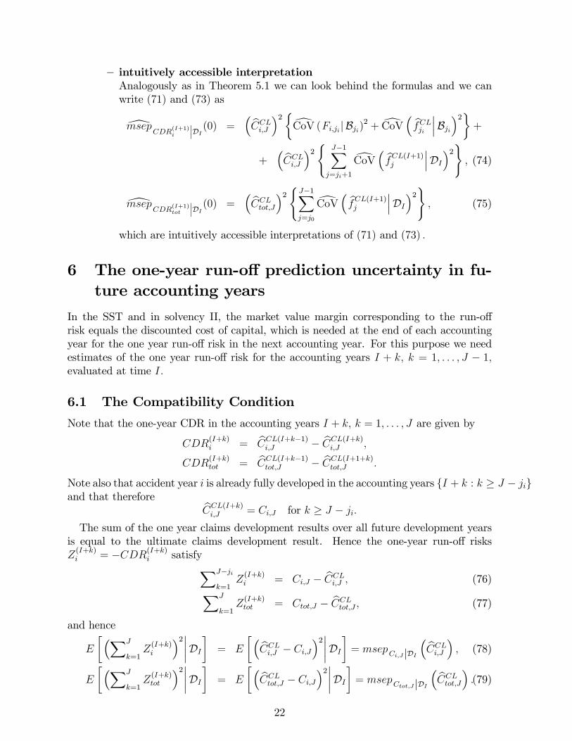
Theorem 6.3 The msep of the one-year run-o¤ risk in future accounting years can beestimated by
i) single accident year i, accounting years I + k + 1; k = 0; : : : ; J � ji � 1
[msepCDR
(I+k+1)i
���DI (0) =� bCCLi;J �2 b�2ji+k� bfCL)ji+k
�28><>: 1
wi;ji+k+
1Xi�1
l=i0wl;ji+k
9>=>;+ (90)
+� bCCLi;J �2
8><>:0B@1 + 1
wi;ji+k
b�2ji+k� bfCLji+k�21CA0B@ J�1Yj=ji+k+1
0B@1 + b(I+k)j
b�2j� bfCLj �21CA� 1
1CA9>=>;
where
b(I+k)j =
wij+k;j�Pij+k�1i=i0
wi;j
��Pij+ki=i0
wi;j
� ; (91)
weights wi;j as de�ned in (4) :
ii) total over all accident years, accounting years I + k + 1; k = 0; : : : ; J � 1
[msepCDR
(I+k+1)tot
���DI (0) =� bCCLtot;J�2
8><>:J�1Y
j=ji+k
0B@1 + b(I+k)j
b�2j� bfCLj �21CA� 1
9>=>; : (92)
iii) The estimators (90) and (92) ful�l the compatibility condition:
Remarks:
- For k = 0 (90) and (92) are of course the same as (68) and (70) in Theorem 5.1.
- The msep for accounting years with k > 0 can also be calculated by �lling up thenext k diagonals with the chain ladder forecasts to get an ari�cial new data set eDI+kand by applying Theorem (70) on the remaining triangle in eDI+k; but by keepingthe estimators b�2j from the original triangle DI :
- (92) is again a surprisingly simple formula.
- intuitively accessible interpretationAnalogously as in Theorem 5.1 the expressions appearing in Theorem 6.3 can beinterpreted in the following easily understandable and intuitively accessible way:
1
wi;ji+k
b�2ji+k� bfCL)ji+k
�2 = dCoV (Fi;ji+kj DI+k)2 ;1Xi�1
l=i0wl;ji+k
b�2ji+k� bfCL)ji+k
�2 = dCoV � bfCLji+k���Bj+k�2 ;b(I+k)j
b�2j� bfCLj �2 = dCoV � bfCL(I+1)j
���DI+k�2 :25

Proof of Theoerm 6.3:The derivation of the estimators in i) was already explained. ii) is obtained analogously.iii) follows from the next Theorem 6.4 and the fact, that the estimators (90) and (92) aregreater than the estimators (93) and (94) : 2
As in section 5 the estimators in Theorem 6.3 can again be approximated by a �rstTaylor approximation.
Theorem 6.4 The msep of the one-year run-o¤ risk in future accounting years can al-ternatively (Taylor approximation) be estimated by
i) single accident year i, accounting years I + k + 1; k = 0; : : : ; J � ji � 1
[msepCDR
(I+k+1)i
���DI (0) =� bCCLi;J �2 b�2ji+k� bfCLji+k�2
8><>:0B@ 1
wi;ji+k+
1Xi�1
l=i0wl;ji+k
1CA9>=>;+
+� bCCLi;J �2
8><>:J�1X
j=ji+k+1
b(I+k)j
b�2j� bfCLj �29>=>; (93)
where b(I+k)j are given by (91).
ii) total over all accident years, accounting years I + k + 1; k = 0; : : : ; J � 1
[msepCDR
(I+k+1)tot
���DI (0) =� bCCLtot;J�2
8><>:J�1X
j=j0+k
b(I+k)j
b�2j� bfCLj �29>=>; (94)
where b(I+k)j is given by (91).
iii) the estimators (93) and (94) ful�l the splitting property:
Remarks:
- The �rst bullet point in the remarks after Theorem 6.3 is analogously valid here.
- (93) and (94) are di¤erent to the Merz-Wüthrich formulas (100) and (101) : Howeverthey give the same numerical results. This cannot be a pure coincidence. Thus theymust be same just written di¤erently.
- The �rst summand in (93) re�ects again the risk that the observation on the nextdiagonal will deviate from the forecast at time I, whereas the second summandentails the risk of updating the forecasts of the later development years: The �rstsummand looks similar to the one in Merz-Wüthrich, but note, that there is adi¤erence even in this �rst summand.
- (94) is again a surprisingly simple formula compared to the rather complicatedexpression with all the covariance terms in (101) :
26

- intuitively accessible interpretationAnalogously as in Theorem 5.1 (93) and (94) can be written as
[msepCDR
(I+k+1)i
���DI (0) =� bCCLi;J �2��dCoV (Fi;ji+kj Bji+k)�2 + dCoV � bfCLji+k���Bji+k�2�+
+� bCCLi;J �2
(J�1X
j=ji+k+1
dCoV � bfCL(I+1+k)j
���DI+k�2) ;[msep
CDR(I+k+1)tot
���DI (0) =� bCCLtot;J�2
(J�1X
j=ji+k
dCoV � bfCL(I+k+1)j
���DI+k�2) ;which are intuitively accessible and understandable formulas.
Proof of Theorem 6.4:(93) and (94) are obtained by a straightforward �rst order Taylor approximation from(90) and (92) :The proof of the splitting property iii) is given in appendix D 2
7 Numerical example
Table 1 shows in the upper left part the data of a claims development triangle of medicalcosts in accident insurance and in the lower right part the chain-ladder forecasts. Column20 contains the CL-forecasts of the ultimate claims (in red) and the corresponding chain-ladder reserves. The total reserves at the end of 2010 for this line of business amounts toCHF 66.697 mio.
0 1 2 3 4 5 6 7 8 9 10 11 12 13 14 15 16 17 18 19 20 Reserves
1984 1'324 2'230 2'373 2'465 2'505 2'559 2'593 2'683 2'755 2'849 2'968 2'999 3'096 3'333 3'420 3'532 3'678 3'724 3'797 3'875 3'9661985 1'430 2'796 3'042 3'136 3'231 3'400 3'526 3'582 3'872 3'905 3'966 4'064 4'388 4'586 4'914 5'394 5'495 5'597 5'719 5'824 6'0031986 1'612 2'970 3'244 3'352 3'412 3'469 3'568 3'618 3'659 3'680 3'698 3'729 3'751 3'787 3'793 3'799 3'815 3'824 3'837 3'851 3'8581987 2'075 3'458 3'724 3'820 3'864 3'938 3'974 3'997 4'017 4'048 4'059 4'100 4'120 4'127 4'144 4'157 4'201 4'222 4'233 4'246 4'2531988 2'673 4'457 4'866 4'960 5'055 5'087 5'135 5'171 5'258 5'407 5'431 5'451 5'465 5'485 5'497 5'507 5'519 5'541 5'568 5'582 5'6041989 2'918 4'730 5'138 5'302 5'359 5'437 5'501 5'550 5'569 5'600 5'605 5'608 5'610 5'653 5'672 5'703 5'742 5'771 5'776 5'794 5'8041990 3'052 4'900 5'371 5'600 5'734 5'812 5'865 5'932 5'980 6'058 6'118 6'141 6'217 6'264 6'309 6'354 6'391 6'408 6'429 6'447 6'5011991 2'649 4'340 4'805 4'995 5'097 5'163 5'315 5'375 5'500 5'586 5'635 5'697 5'731 5'758 5'804 5'834 5'859 5'880 5'893 5'900 5'961 611992 2'779 4'834 5'283 5'498 5'629 5'670 5'738 5'808 5'835 5'935 6'028 6'059 6'092 6'111 6'143 6'169 6'186 6'200 6'216 6'256 6'321 1051993 2'492 4'344 4'782 4'968 5'033 5'107 5'191 5'230 5'266 5'349 5'388 5'399 5'431 5'459 5'466 5'471 5'475 5'477 5'512 5'548 5'605 1281994 3'026 5'403 5'820 6'063 6'137 6'197 6'254 6'512 6'610 6'750 6'851 6'910 6'977 7'059 7'156 7'217 7'263 7'302 7'348 7'396 7'473 2101995 4'154 7'574 8'418 8'836 9'099 9'276 9'440 9'591 9'825 10'038 10'187 10'361 10'479 10'564 10'647 10'776 10'865 10'923 10'993 11'065 11'179 4031996 3'490 6'266 7'052 7'375 7'505 7'646 7'746 7'809 7'860 7'894 7'922 7'947 7'976 8'046 8'110 8'221 8'289 8'334 8'387 8'442 8'529 4191997 3'557 7'089 7'812 8'065 8'303 8'445 8'542 8'616 8'697 8'744 8'816 8'874 8'946 9'008 9'108 9'233 9'309 9'359 9'419 9'481 9'579 5701998 4'742 8'819 9'821 10'355 10'662 11'000 11'288 11'509 11'650 11'771 11'890 11'983 12'087 12'225 12'361 12'530 12'633 12'701 12'783 12'866 12'999 9121999 6'508 11'826 13'199 13'889 14'277 14'574 14'855 15'140 15'332 15'469 15'628 15'758 15'930 16'112 16'291 16'514 16'650 16'740 16'847 16'956 17'132 1'3742000 6'708 13'382 15'155 15'797 16'130 16'389 16'658 16'865 17'040 17'205 17'321 17'461 17'652 17'853 18'051 18'299 18'450 18'549 18'668 18'789 18'983 1'6622001 6'283 11'983 13'552 14'280 14'625 14'956 15'180 15'281 15'364 15'474 15'624 15'750 15'922 16'104 16'283 16'506 16'642 16'732 16'839 16'948 17'123 1'6492002 6'297 12'810 14'166 14'883 15'326 15'568 15'731 15'973 16'062 16'253 16'411 16'543 16'724 16'915 17'103 17'337 17'480 17'574 17'687 17'802 17'986 1'9242003 6'369 12'594 14'450 15'191 15'561 15'902 16'050 16'186 16'386 16'581 16'742 16'878 17'062 17'257 17'448 17'687 17'833 17'929 18'044 18'161 18'349 2'1632004 7'735 15'339 17'274 18'177 18'783 19'247 19'584 19'850 20'096 20'335 20'532 20'698 20'925 21'163 21'398 21'691 21'870 21'988 22'129 22'272 22'503 2'9182005 9'022 17'415 19'896 21'148 22'027 22'522 22'874 23'184 23'471 23'751 23'981 24'175 24'439 24'718 24'992 25'335 25'544 25'681 25'846 26'014 26'283 3'7612006 10'311 21'215 24'530 26'123 27'200 27'736 28'170 28'551 28'905 29'250 29'533 29'772 30'098 30'441 30'778 31'201 31'458 31'627 31'829 32'036 32'368 5'1682007 10'945 21'346 23'646 24'651 25'341 25'841 26'245 26'600 26'930 27'251 27'515 27'738 28'041 28'361 28'675 29'069 29'308 29'466 29'654 29'847 30'156 5'5052008 12'073 22'274 25'170 26'390 27'129 27'664 28'096 28'477 28'830 29'173 29'456 29'694 30'019 30'361 30'698 31'119 31'376 31'544 31'746 31'953 32'283 7'1132009 10'667 21'295 23'857 25'013 25'714 26'221 26'631 26'991 27'326 27'652 27'920 28'145 28'453 28'778 29'097 29'496 29'739 29'899 30'090 30'286 30'599 9'3042010 12'385 23'476 26'299 27'574 28'346 28'905 29'357 29'755 30'123 30'483 30'778 31'027 31'366 31'724 32'076 32'516 32'784 32'960 33'171 33'387 33'732 21'347
Total 66'697fj
CL 1.896 1.120 1.048 1.028 1.020 1.016 1.014 1.012 1.012 1.010 1.008 1.011 1.011 1.011 1.014 1.008 1.005 1.006 1.007 1.010
Table 1: triangel of cumulative payments in CHF 1'000 and CLforecasts
27

Table 2 shows the square root of the estimated msep for the ultimate run-o¤ and forthe one year run-o¤ in the next accounting year where the latter is calculated with the"exact" estimator according to Theorem 5.1 as well as with the Taylor approximationaccording to Theorem 5.2. We see, that in this example the numerical results of the twoestimators di¤er not more than in the second digit after the decimal point and that theresults with the "exact" estimator are greater, but only very minor in the second digitafter the decimal point.
Reservesmsep1/2 in % reserves
in % reservesexact Taylor appr
1991 61 71 116% 70.74 70.74 116%1992 105 87 82% 47.58 47.58 45%1993 128 92 72% 45.87 45.87 36%1994 210 115 55% 40.51 40.51 19%1995 403 169 42% 88.48 88.48 22%1996 419 238 57% 190.98 190.98 46%1997 570 289 51% 139.94 139.94 25%1998 912 378 41% 163.51 163.51 18%1999 1'374 482 35% 198.78 198.78 14%2000 1'662 517 31% 106.76 106.76 6%2001 1'649 493 30% 110.51 110.51 7%2002 1'924 516 27% 120.35 120.35 6%2003 2'163 549 25% 187.36 187.36 9%2004 2'918 632 22% 155.02 155.02 5%2005 3'761 703 19% 160.31 160.31 4%2006 5'168 814 16% 201.54 201.54 4%2007 5'505 798 14% 224.48 224.48 4%2008 7'113 862 12% 265.29 265.29 4%2009 9'304 930 10% 437.82 437.81 5%2010 21'347 1'795 8% 1'507.37 1'507.36 7%Total 66'697 5'033 8% 2'435.88 2'435.86 4%
Table 2
acci
dent
yea
r
ultimate runoff one year runoff
msep1/2next accounting year
Table 3 shows the results obtained for the square-root of the one-year msep in futureaccounting years until �nal development together with the ingoing reserves. The numericalresults obtained with the "exact" formula and with the Taylor approximation are againpractically the same with di¤erences only in the second digit after the decimal point.From the table we can also the splitting property of the Taylor-approximation.In the current formula for calculating the risk margin in solvency II it assumed that
the required capital for the remaining one-year run-o¤ risk in future accounting yearsdecreases proportionally to the remaining reserves. This was due to the lack of formulasto calculate the prediction uncertainty for future accounting years. But now the formulashave been developed and are here. Comparing the development pattern of the reserveswith the development pattern of the msep we see, that the latter decreases much slower.This is not a surprise. Complex and complicated claims such as severe bodily injuryclaims stay open for a long time, whereas "normal" claims can be settled much quicker.Hence the proportion of the reserves stemming from complex claims is bigger in laterdevelopment years. But the prediction uncertainty of this kind of claims is bigger as forthe "normal" claims. But it also means that one will need more capital in solvency IIwith this new formulas, since the risk margin will become bigger.
28

in 1'000 dev. patterndev.pattern
"exact" Taylor appr.
2011 66'697 100% 2'435.88 2'435.86 100%2'012 48'513 73% 1'801.67 1'801.67 74%2'013 40'919 61% 1'661.06 1'661.05 68%2'014 35'786 54% 1'564.28 1'564.27 64%2'015 31'614 47% 1'426.15 1'426.14 59%2'016 27'960 42% 1'250.72 1'250.71 51%2'017 24'694 37% 1'163.14 1'163.14 48%2'018 21'662 32% 1'099.81 1'099.81 45%2'019 18'791 28% 1'027.23 1'027.23 42%2'020 16'067 24% 953.60 953.60 39%2'021 13'531 20% 874.67 874.67 36%2'022 11'164 17% 788.65 788.65 32%2'023 8'933 13% 692.48 692.48 28%2'024 6'930 10% 602.20 602.20 25%2'025 5'164 7.7% 518.85 518.85 21%2'026 3'648 5.5% 341.16 341.16 14%2'027 2'494 3.7% 274.70 274.70 11%2'028 1'611 2.4% 244.81 244.81 10%2'029 874 1.3% 198.87 198.87 8%2'030 345 0.5% 162.87 162.87 7%
sum 1year msep 25'326'904ultimate msep 25'326'904
ingoing Reserves one year runoff
development pattern reserves and mseptotal over all accident years
msep1/2
Table 3
acco
untin
g ye
ar
0
0.1
0.2
0.3
0.4
0.5
0.6
0.7
0.8
0.9
1
1 2 3 4 5 6 7 8 9 10 11 12 13 14 15 16 17 18 19 20
dev. Pattern ingoing reservs dev. pattern msep
AcknowledgementI am grateful to Ancus Röhr. Discussions with him on earlier drafts of his paper [12]
have motivated me to work further on this topic. The result is the present paper. I am alsograteful to Hans Bühlmann. He told me that Lemma 3.5 is called the telescope-formulaand how it can be proved best. Finally I would like to thank Patrick Helbling, who haddone most of the calculations of the numerical example.
29
References
[1] Buchwalder M., Bühlmann, H., Merz M., Wüthrich M. (2006). The Mean Square Error ofPrediction in the Chain Ladder Reserving Method-Final Remark 36/2, 521-542.
[2] Buchwalder M., Bühlmann, H., Merz M., Wüthrich M. (2006). The Mean Square Error ofPrediction in the Chain Ladder Reserving Method (Mack and Murphy Revisited).ASTINBulletin 36/2, 553.
[3] Bühlmann, H., De Felice M., Gisler, A., Moriconi F., Wüthrich, M.V. (2009). RecursiveCredibility Formula for Chain Ladder Factors and the Claims Development Result. ASTINBulletin 39/1,275-306.
[4] Gisler, A. (2006). The estimation error in the chain-ladder reserving method: a Bayesianapproach. ASTIN Bulletin 36/2, 554-565.
[5] Gisler, A. , Wüthrich M.V.
[6] (2008). Credibility for the chain-ladder reserving method.38/2, 565-600.
[7] Mack, T. (1993). Distribution-free calculation of the standard error of chain ladder reserveestimates. ASTIN Bulletin 23/2, 213�225.
[8] Mack, T., Quarg B., Braun C. (2006).The Mean Square Error of Prediction in the ChainLadder Reserving Method- A Comment. ASTIN Bulletin 36/2, 523-552.
[9] Merz M., Wüthrich M.V. (2008). Stochastic Claims Reserving Methods in Insurance, Wiley.
[10] Merz M., Wüthrich M.V. (2008). Modelling the claims development result for solvencypurposes. CAS Forum, Fall 2008, 542-568.
[11] Merz M., Wüthrich M.V. (2014). Claims run-o¤ uncertainty: the full picture, SSRN man-uscript 2524352.
[12] Roehr A. (2016). Chain ladder and error propagation, to appear in the next ASTIN Bulletin.
30

Appendices
A Formulae of Mack and Merz-Wüthrich
A.1 Formula of Mack
Written in the notation of this paper Mack [7] has found the following formulas for esti-mating the total run-o¤ uncertainties for the CL reserves.
Theorem A.1 (Mack) The msep can be estimated by
i) single accident year i
[msepCi;J jDI� bCCLi;J � = � bCCLi;J �2 J�1X
j=ji
b�2j� bfCLj �2 1
wi;j+
1Pij�1i=i0
wi;j
!(95)
where bCCLi;j are the CL-forecasts and where wi;j are as de�ned in (4) :ii) total over all accident years
[msepCtot;J jDI� bCCLtot;J� = IX
i=iJ+1
[msepCi;J jDI� bCCLi;J � (96)
+ 2IX
i=iJ+1
bCCLi;J
IXk=i+1
bCCLk;J!
J�1Xj=ji
0B@ b�2j� bfCLj �2 1Pij�1m=i0
wm;j
1CA :A.2 Formulae of Merz-Wüthrich
In [10] Merz and Wüthrich found the following formula for the msep of the one yearrun-o¤ risk in the next accounting year (see formulas (1.2) and (2.3) in [11]).
Theorem A.2 The msep of the one-year run-o¤ risk in the next accounting year can beestimated by
i) single accident year i
[msepCDRi;I+1jDI (0) =� bCCL(I)i;J
�2 b�2ji� bfCL(I)ji
�2
1
wi;ji+
1Pij�1k=i0
wk;ji
!(97)
+� bCCL(I)i;J
�2 J�1Xj=ji+1
b�2j� bfCL(I)j
�2 �(I)j
1Pij�1k=i0
wk;j
!;
where�(I)j =
wij ;jPijk=i0
wk;j: (98)
31

ii) total over all accident years
[msepCDRtot;I+1jDI (0) =IX
i=iJ+1
[msepCDRi;I+1jDI (0) (99)
+2
IXi=iJ+1
IXm=i+1
bCCL(I)i;JbCCL(I)m;J
8><>: b�2ji� bfCL(I)ji
�2 1Pi�1l=i0
wl;ji+
J�1Xj=ji+1
b�2j� bfCL(I)j
�2�(I)j 1Pij�1k=i0
wk;j
9>=>; :In [11] Merz and Wüthrich also derived the following formulas for estimating the msep
of the one year run-o¤ risk in future accounting years (see formulas (1.4) and (2.4) in[11]).
Theorem A.3 The msep of the one-year run-o¤ risk of future accounting years I+1+kcan be estimated by
i) single accident year i (for k = 1; : : : ; J � ji � 1)
[msepCDRi;I+k+1jDI (0) =
=� bCCLi;J �2 b�2ji+k� bfCLji+k�2
1bCCLi;ji+k +
kYm=1
�1� �(I)ji+m
� 1Pi�1�km=i0
wm;ji+k
!(100)
+� bCCLi;J �2 J�1X
j=ji+k+1
b�2j� bfCLj �2 �(I)j�k
k�1Ym=0
�1� �(I)j�m
� 1Pij�1m=i0
wm;j
!:
ii) total over all accident years (for k = 1; : : : ; J � 1)
[msepCDRtot;I+k+1jDI (0) =IX
i=iJ+k+1
[msepCDRi;I+k+1jDI (0)
+2
IXi=iJ+k+1
IXm=i+1
bCCLi;J bCCLm;J b�2ji+k� bfCLji+k�2kY
m=1
�1� �(I)ji+m
� 1Pi�k�1m=i0
wm;ji+k(101)
+2
IXi=iJ+k+1
IXm=i+1
bCCLi;J bCCLm;J J�1Xj=ji+k+1
b�2j� bfCLj �2 �(I)j�k
k�1Ym=0
�1� �(I)j�m
� 1Pij�1l=i0
wl;j
!:
32
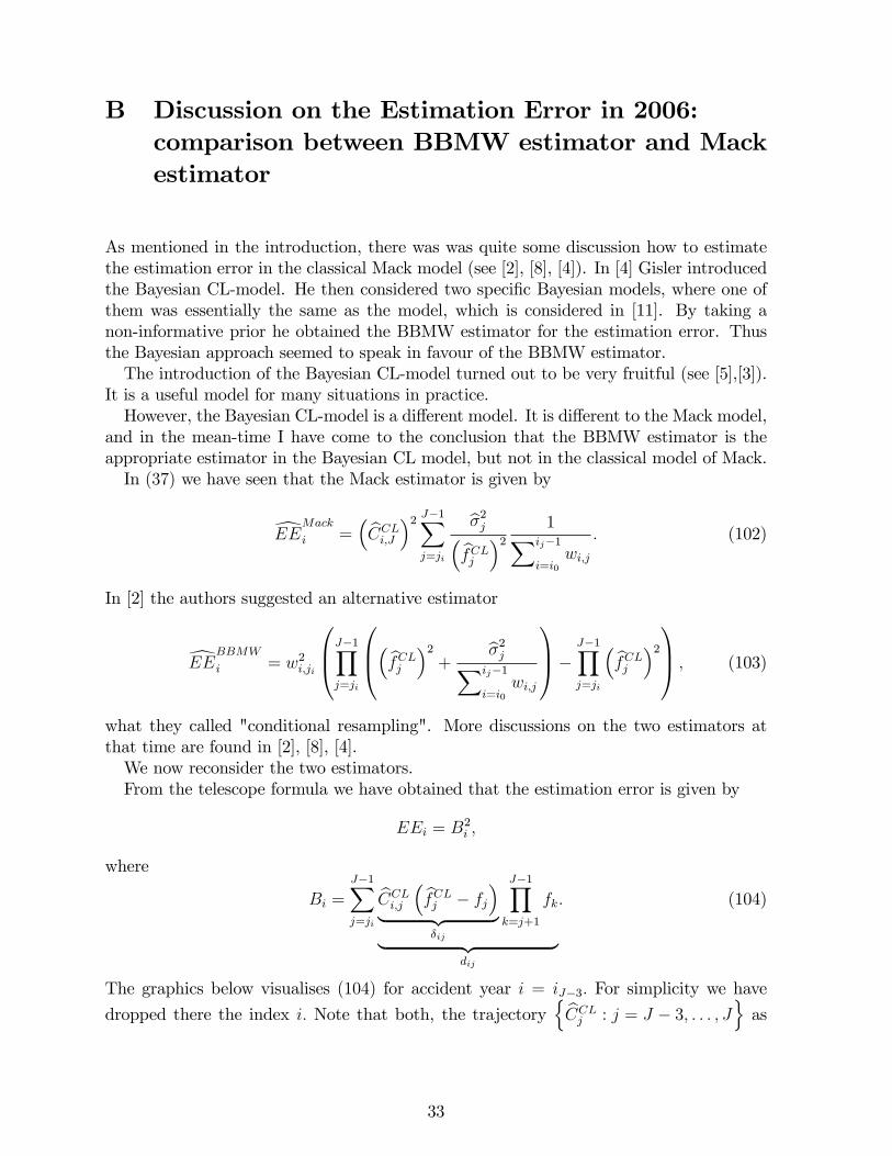
B Discussion on the Estimation Error in 2006:comparison between BBMW estimator and Mackestimator
As mentioned in the introduction, there was was quite some discussion how to estimatethe estimation error in the classical Mack model (see [2], [8], [4]). In [4] Gisler introducedthe Bayesian CL-model. He then considered two speci�c Bayesian models, where one ofthem was essentially the same as the model, which is considered in [11]. By taking anon-informative prior he obtained the BBMW estimator for the estimation error. Thusthe Bayesian approach seemed to speak in favour of the BBMW estimator.The introduction of the Bayesian CL-model turned out to be very fruitful (see [5],[3]).
It is a useful model for many situations in practice.However, the Bayesian CL-model is a di¤erent model. It is di¤erent to the Mack model,
and in the mean-time I have come to the conclusion that the BBMW estimator is theappropriate estimator in the Bayesian CL model, but not in the classical model of Mack.In (37) we have seen that the Mack estimator is given by
dEEMack
i =� bCCLi;J �2 J�1X
j=ji
b�2j� bfCLj �2 1Xij�1
i=i0wi;j
: (102)
In [2] the authors suggested an alternative estimator
dEEBBMW
i = w2i;ji
0B@J�1Yj=ji
0B@�bfCLj �2+
b�2jXij�1
i=i0wi;j
1CA� J�1Yj=ji
� bfCLj �21CA ; (103)
what they called "conditional resampling". More discussions on the two estimators atthat time are found in [2], [8], [4].We now reconsider the two estimators.From the telescope formula we have obtained that the estimation error is given by
EEi = B2i ;
where
Bi =
J�1Xj=ji
bCCLi;j � bfCLj � fj�
| {z }�ij
J�1Yk=j+1
fk
| {z }dij
: (104)
The graphics below visualises (104) for accident year i = iJ�3: For simplicity we have
dropped there the index i: Note that both, the trajectoryn bCCLj : j = J � 3; : : : ; J
oas
33

well as the trajectory��j:= E [Ci;jj DI ] : j = J � 3; : : : ; J
; are �xed and non stochastic.
To estimate B2i we should have in mind that the �ij are realisations of r.v.
�ij = bCCLi;j (Fj � fj) (105)
where Fj =
ij�1Xi=i0
wi;jw�;j
Fi;j; w�;j =
ij�1Xi=i0
wi;j :
and that�2ij = E
��2ij
��DI� :Since bCCLi;j is a known and given multiplicative factor it is obvious that one should considerthe conditional distribution of �ij given Bj for estimating �2ij: This is exactly what Mackdoes, and he obtains
E��2ij
��Bj� =� bCCLi;j �2 �2jXij�1
i=i0wi;j
;
b�2(Mack)
ij = bE ��2ij
��Bj� = � bCCLi;j �2 b�2jXij�1
i=i0wi;j
: (106)
Since f�i;j0 ; : : :�i;j�1g are conditional on Bj known constants, it follows that the r.v.f�ijj Bj : j = ji; : : : ; J � 1g are uncorrelated. Hence fdij : j = ji; : : : ; J � 1g can be con-sidered as realisations of uncorrelated r.v. which then leads immediately to the Mackestimator (102) :In terms of the telescope formula, the BBMW estimator is obtained if one considers
the r.v. eBi = J�1Xj=ji
eCi;j � eFj � fj� J�1Yk=j+1
fk: (107)
34

where
eCi;j = wi;jj j�1Yk=ji
eFk and where
the eFj are independent r.v. with E h eFji = fj and Var (Fjj Bj) = �2jXij�1
i=i0wi;j
:
Hence the known multiplicative constants bCCLi;j in (104) are replaced by r.v. eCi;j in(107) ;which hardly makes sense in the classical Mack model.However, in the Bayesian CL-model the CL factors fj are realisations of r.v. FBj (the
superscript B indicates that we are in the Bayesian model). The estimation error is thengiven by
EEi = B�2i ;
where
B�i =�E [Ci;J j DI ]�dCi;JCL�
= wi;ji
J�1Yj=ji
FBj �J�1Yj=ji
bfCLj!: (108)
With the telescope formula we also obtain that
B�i =XJ�1
j=ji
eC�i;j �FBj � bfCLj �YJ�1
k=j+1
bfCLk ; (109)
where eC�i;j = wi;jj jYk=ji
FBk :
which should be compared with (104) : In the following we always refer to the BayesianCL-model considered in [11]. In this model the r.v. FBj are conditional onDI independent.By taking a non informative prior and in the cases where the two �rst moments of theposterior distribution exist, these moments are given by
E�FBj��DI� = bfCLj ; (110)
Var�FBj��DI� =
�2jXij�1
i=i0wi;j
: (111)
From (108) ; (110) ; (111) and the conditional independence of the FBj we immediately seethat
EhB�
2
i
���DIi = w2i;ji0B@J�1Yj=ji
0B@�bfCLj �2+
�2jXij�1
i=i0wi;j
1CA� J�1Yj=ji
� bfCLj �21CA :Hence, the BBMW estimator is the appropriate estimator in the Bayesian CL-model, butnot in the classical model of Mack.
35
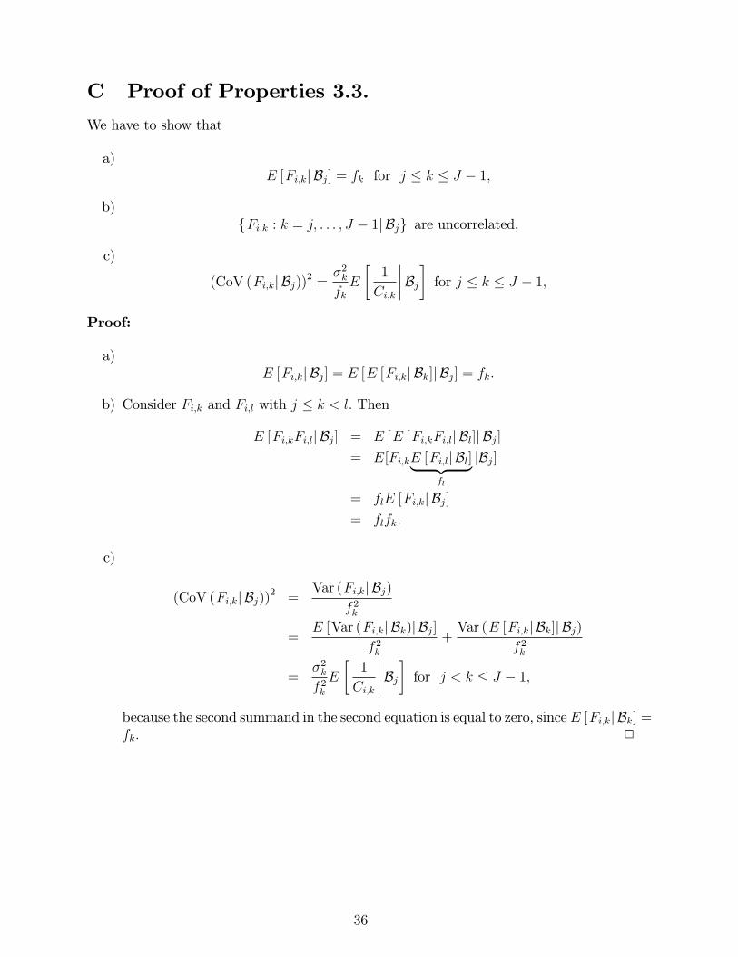
C Proof of Properties 3.3.
We have to show that
a)E [Fi;kj Bj] = fk for j � k � J � 1;
b)fFi;k : k = j; : : : ; J � 1j Bjg are uncorrelated,
c)
(CoV (Fi;kj Bj))2 =�2kfkE
�1
Ci;k
����Bj� for j � k � J � 1;Proof:
a)E [Fi;kj Bj] = E [E [Fi;kj Bk]j Bj] = fk:
b) Consider Fi;k and Fi;l with j � k < l: Then
E [Fi;kFi;lj Bj] = E [E [Fi;kFi;lj Bl]j Bj]= E[Fi;kE [Fi;lj Bl]| {z }
fl
jBj]
= flE [Fi;kj Bj]= flfk:
c)
(CoV (Fi;kj Bj))2 =Var (Fi;kj Bj)
f 2k
=E [Var (Fi;kj Bk)j Bj]
f 2k+Var (E [Fi;kj Bk]j Bj)
f 2k
=�2kf 2kE
�1
Ci;k
����Bj� for j < k � J � 1;because the second summand in the second equation is equal to zero, sinceE [Fi;kj Bk] =fk: 2
36

D Theorem 6.4: Proof of the splitting property iii)
Proof:
i) single accident year i
J�ji�1Xk=0
[msepCDR
(I+k+1)i
���DI (0)
=� bCCLi;J �2
8><>:J�ji�1Xk=0
b�2ji+k� bfCLji+k�20B@ 1
wi;ji+k+
1Xi�1
l=i0wl;ji+k
1CA +
J�1Xj=ji+k+1
b(I+k)j
b�2j� bfCLj �29>=>;
=� bCCLi;J �2 J�1X
j=ji
b�2j� bfCLj �20BBBBBB@1
wi;j+
1Xi�1
l=i0wl;j
+
j�ji�1Xk=0
b(I+k)j
| {z }Bi;j
1CCCCCCA : (112)
By plugging (91) into (112) we obtain
Bi;ji =1Xi�1
l=i0wl;j
;
Bi;ji+1 = Bi;ji +wi�1;jXi�1
l=i0wl;j
Xi�2
l=i0wl;j
=1Xi�1
l=i0wl;j
+wi�1;jXi�1
l=i0wl;j
Xi�2
l=i0wl;j
=1Xi�2
l=i0wl;j
=1Xiji+1�1
l=i0wl;j
...
Bi;ji+k =1Xi�k�1
l=i0wl;j
=1Xiji+k�1
l=i0wl;j
(113)
Hence
J�ji�1Xk=0
[msepCDR
(I+k+1)i
���DI (0) =� bCCLi;J �2 J�1X
j=ji
b�2j� bfCLj �20B@ 1
wi;j+
1Xij�1
l=i0wl;j
1CA ;which is identical to (44) :
37

ii) Total over all accident years
Ji�1Xk=0
[msepCDR
(I+k+1)tot
���DI (0 =� bCCLtot;J�2
8><>:Ji�1Xk=0
J�1Xj=j0
b(I+k)j
b�2j� bfCLj �29>=>;
=
8><>:�bCCLtot;J�2 J�1X
j=j0
b�2j� bfCLj �2 j�j0Xk=0
b(I+k)j| {z }
9>=>;Bj
:
Since jI = j0 we see from (113) and the de�nition of Bi;j in (112) that
Bj =1Xij�1
l=i0wl;j
��1
wI;j� b(I)j
�
=1Xij�1
l=i0wl;j
�
0B@ 1XI�1
l=i0wl;j
� wI;j�XI�1
l=i0wl;j
��XI�1
l=i0wl;j
�1CA
=1Xij�1
l=i0wl;j
� 1XI
l=i0wl;j
=
XI
l=ijwl;jXI
l=i0wl;j
1Xij�1
l=i0wl;j
=
XI
l=ij
bCCLl;;jbCCLtot;;j 1Xij�1
l=i0wl;j
:
Hence
Ji�1Xk=0
[msepCDR
(I+k+1)tot
���DI (0 =� bCCLtot;J�2
0B@J�1Xj=j0
b�2j� bfCLj �2 1Xij�1
l=i0wl;j
qj
1CA ; (114)
where
qj =
XI
l=ij
bCCLl;;jbCCLtot;;j :
(114) is identical to(46). 2
38


![Untitled-1 [cdn.kitsune.tools] · Industrial Ladder Scaffold FRP Stool Ladder Aluminum Ladder Aluminium Tiltable Step FRP Wall Supporting Aluminum Wall Supporting Tanker Ladder —self](https://img.pdfslide.us/doc/110x75/5f0ebf297e708231d440bd69/untitled-1-cdn-industrial-ladder-scaffold-frp-stool-ladder-aluminum-ladder-aluminium.jpg)