The CGR4 lightning sensor - Bureau of Meteorology · 2010-03-09 · the lightning flash and the fraction of flashes counted at that distance is a feature of the sensor known as its

$Page 1: The CGR4 lightning sensor - Bureau of Meteorology · 2010-03-09 · the lightning flash and the fraction of flashes counted at that distance is a feature of the sensor known as its$
263

Australian Meteorological and Oceanographic Journal 58 (2009) 263-273

Introduction

Lightning flash counters (LFC) of various types have been used for several decades to obtain climatological informa-tion on lightning occurrence (Prentice 1974; Prentice and Mackerras 1969; Anderson et al. 1979; Barham 1965; Barham and Mackerras 1972). Subsequently, a new class of lightning sensor known as CGRx with a relatively short range, less than 20 km, was designed to identify the type of lightning as negative ground flash (NGF), positive ground flash (PGF), or cloud flash (CF), and to obtain objective measures of the cloud flash-to-ground flash ratio, hence the acronym CGRx for ‘Cloud Ground Ratio’ version x. The CGR1 was described by Mackerras (1985), CGR2 was a transitional version, and CGR3 was the version used from about 1986 onward. The CGR3 version included the features described by Mackerras (1985) together with separate positive ground flash detec-tion (Baral and Mackerras 1993). The CGR3 was based on

hard-wired analogue and logic circuitry. In the early 2000s, tests commenced on a modified form of the sensor, denoted CGR4, using a microprocessor to replace most of the hard-wired logic and all the electromechanical registers. We con-sider here the design and performance of the CGR4 light-ning sensor, the observational basis for assigning lightning events to the categories NGF, PGF and CF, the rules imple-mented to make the assignments, and the estimated rates of incorrect flash type assignment. The form of the CGR4 sensor that implements the flash classification algorithms described here was developed in response to a requirement of the Australian Bureau of Me-teorology for a low cost lightning sensor to replace its legacy CIGRE 500 Hz lightning flash counters (LFC) (Kuleshov and Jayaratne 2004). Its specifications included a detection range similar to that of a human observer for detecting thunder, the ability to discriminate between the three lightning event types, and an interface compatible with current and future generation automatic weather stations (AWS). The lightning climatology accumulated after the CGR4s are deployed will

The CGR4 lightning sensor

D. Mackerras1, M. Darveniza1,2 and P. Hettrick3

1Lightning and Transient Protection Pty Ltd 2University of Queensland

3Australian Bureau of Meteorology(Manuscript received March 2009; revised October 2009)

The design of the CGR4 lightning sensor is based on several observed charac-teristics of the electric field changes caused by nearby lightning, and the radio-frequency noise bursts from lightning. The electric field signals from lightning are detected by a simple aerial, and processed by a combination of analogue and digi-tal circuitry under microprocessor control to determine if there is a nearby light-ning flash, and, if so, to assign the type of flash as negative ground flash (NGF), positive ground flash (PGF), or cloud flash (CF). These types have distinctive fea-tures in their electric field change waveforms, enabling an assignment of type of lightning to be made by obtaining several measures of the waveform character-istics and applying an appropriate set of rules. A method of estimating the sen-sor’s effective range and area has been developed using data for a set of nearby lightning events. This involves the recording of the variation of electric field with time, the response of a lightning sensor, and the distance to the lightning flash us-ing thunder ranging. As the sensor is able to apply different threshold overall field changes for each type of lightning detected, a single effective range of 11.3 km (effective area 400 km2) for all types of lightning was achieved by using threshold field changes of 520 volts per metre (V/m) for CF, 760 V/m for NGF, and 1200 V/m for PGF. The sensor responds to about 90 per cent of all flashes at 8 km, about 40 per cent at 11 km, and approaching zero above 16 km.

Corresponding author address: D. Mackerras, 249 Swann Rd, Taringa, Qld 4068, Australia.Email: [email protected]

264 Australian Meteorological and Oceanographic Journal 58:4 December 2009

include lightning flash type information absent from the CI-GRE LFC record. The ability of the CGR4 to interface with an AWS enables deployment to remote areas and so will enable a higher sensor network density to be achieved than with the CIGRE LFC. The relationship between the distance from the sensor to the lightning flash and the fraction of flashes counted at that distance is a feature of the sensor known as its performance curve. This provides estimates of the effective range and hence area, and this enables the lightning flash density (mea-sured in events per unit area and per year) to be calculated from the annual event counts. The effective range depends on the threshold overall field change selected for the sensor.

Detection of lightning-caused electric field changes (EFC) using simple aerials

As discussed for the early LFC (e.g. Mackerras 1968), the transient electric field changes (EFC) at a remote observation point caused by a lightning discharge may be detected us-ing a simple aerial (antenna) having capacitance to ground, Ca, and effective height, ha. To obtain a voltage signal rep-resenting the EFC, the aerial is connected to a capacitor, C, and a resistor, R, in parallel, connected between the aerial terminal and ground. If the product (ha Ca) and C are known, the time-varying voltage signal, V, can be scaled in terms of the electric field change in V/m, providing the type of record shown in Fig. 1. For this type of lightning sensor, the aerial consists of a vertical PVC pipe, nominally 50 mm inside diameter, about 5 m high, containing a 3150 mm length of aluminium tube, 50 mm outside diameter, with its lower end at a height of 1620 mm above ground level. An insulated wire lead-in con-nects the ‘active’ part of the aerial to the sensor or to an EFC recording system. This aerial was derived from the vertical aerial used with the CIGRE 500 Hz LFC (Prentice et al. 1975), and has the same characteristics, namely:

capacitance to ground, Ca ≈ 58 pF, effective height, ha ≈ 2.4 m,and product (Ca ha) ≈ 140 pFm.

Using this aerial, the electric field change in V/m may be obtained from the output voltage of the aerial filter circuit of the sensor shown in Fig. 2. The processing of the EFC signal is carried out partly in analogue circuitry, and partly digitally. The structure of the operating program controlling the whole process is shown in flow chart form in Fig. 3.

Electric field changes (EFC) caused by various types of lightning

The EFC caused by various types of lightning have been identified by many workers in several countries; see exten-sive reviews by Uman (1987), and Rakov and Uman (2003). Lightning events typically have durations between about 400

and 1200 ms, with an extreme range of about 200 to 1500 ms. Figure 1 gives typical examples of the EFC waveforms re-corded in Brisbane, Australia, for NGF, PGF and CF events. The overall field change, Eo, is the interval between the ex-treme positive and negative excursions of the waveform. The distinctive features of these three types of lightning are de-scribed in various publications summarised below.• Negative ground flash (NGF): the distinguishing EFC

features, see Fig. 1(a), are the presence of positive-going steps, denoted as R-changes, caused by the short-dura-tion high-current strokes that transfer negative charge to ground. There may also be long-duration positive-go-ing ramps in the EFC known as C-changes which usu-ally follow an R-change, and are caused by long-duration low magnitude continuing currents flowing to earth in the discharge channel. NGF events are the most widely documented of all types of lightning, see e.g., Brook and Kitagawa (1960); Kitagawa et al. (1962); Ogawa and Brook (1969); Thomson (1980); and Mackerras (1968).

• Positive ground flash (PGF): these usually have large negative-going ramps with one, or occasionally two, neg-ative-going steps, as shown in Fig. 1(b). The PGF wave-forms usually differ from those of CF waveforms because the larger negative-going step is large compared with Eo.

Fig. 1 Electric field change, E, versus time, t, for three events recorded in Brisbane, Australia.

(a) An NGF event 10.3 km distant, overall field change, Eo, approximately 520 V/m. R denotes R-changes, C denotes a C-change.

(b) A PGF event 5 km distant, Eo about 13 kV/m. NS denotes negative step, NR denotes negative-going ramp.

(c) A CF event 10.3 km distant, Eo about 1.6 kV/m. NR denotes negative-going ramp, K denotes K-change.

Mackerras et al.: The CGR4 lightning sensor 265

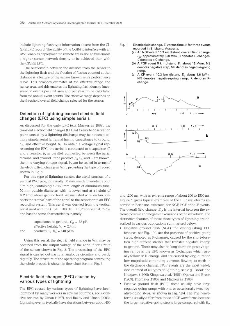
Fig. 2 Block diagram of the CGR4 lightning sensor. The aerial filter circuit consists of CA1, CA2, CA3 and R/2 (or R/24 when switch SW3 is closed). DG1, DG2, DG3 are digital signals controlling analogue switches SW1, SW2, SW3, and discharging Peak Hold sub-circuit storage capacitors. Peak Hold sub-circuits hold the peak value of their input signals for a sufficient time for the value to be digitised. TC = time constant for decay of held voltage, or for the C×R product for high-pass filters. ID1, ID2, ID3, ID4 and ID5 are ideal diode sub-circuits with negligible forward voltage drop when conducting. ADJ. AMPL indi-cates amplifier with adjustable gain, about ×3. CCS = Current Source Signal; SFS = Step Function Signal; these signals are injected during testing to simulate the effect of electric field changes.


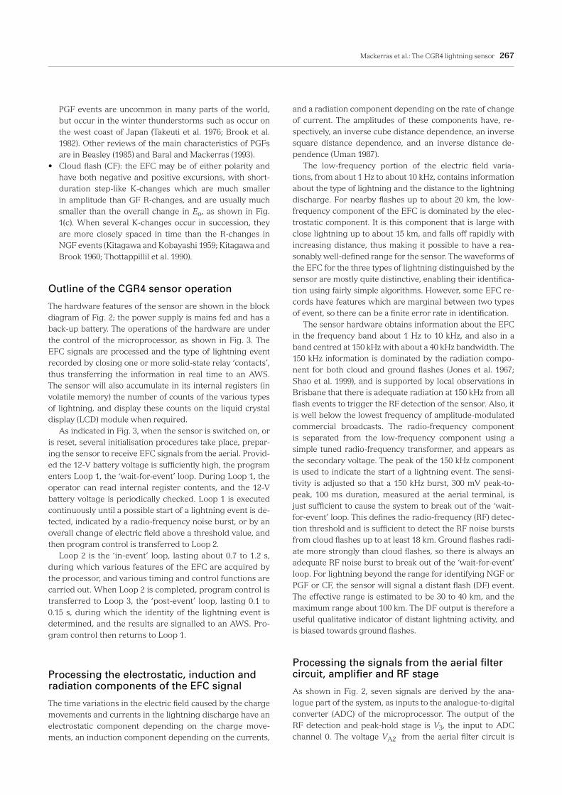
Fig. 3 Flow chart for operating program for the CGR4 lightning sensor.


and a radiation component depending on the rate of change of current. The amplitudes of these components have, re-spectively, an inverse cube distance dependence, an inverse square distance dependence, and an inverse distance de-pendence (Uman 1987). The low-frequency portion of the electric field varia-tions, from about 1 Hz to about 10 kHz, contains information about the type of lightning and the distance to the lightning discharge. For nearby flashes up to about 20 km, the low-frequency component of the EFC is dominated by the elec-trostatic component. It is this component that is large with close lightning up to about 15 km, and falls off rapidly with increasing distance, thus making it possible to have a rea-sonably well-defined range for the sensor. The waveforms of the EFC for the three types of lightning distinguished by the sensor are mostly quite distinctive, enabling their identifica-tion using fairly simple algorithms. However, some EFC re-cords have features which are marginal between two types of event, so there can be a finite error rate in identification. The sensor hardware obtains information about the EFC in the frequency band about 1 Hz to 10 kHz, and also in a band centred at 150 kHz with about a 40 kHz bandwidth. The 150 kHz information is dominated by the radiation compo-nent for both cloud and ground flashes (Jones et al. 1967; Shao et al. 1999), and is supported by local observations in Brisbane that there is adequate radiation at 150 kHz from all flash events to trigger the RF detection of the sensor. Also, it is well below the lowest frequency of amplitude-modulated commercial broadcasts. The radio-frequency component is separated from the low-frequency component using a simple tuned radio-frequency transformer, and appears as the secondary voltage. The peak of the 150 kHz component is used to indicate the start of a lightning event. The sensi-tivity is adjusted so that a 150 kHz burst, 300 mV peak-to-peak, 100 ms duration, measured at the aerial terminal, is just sufficient to cause the system to break out of the ‘wait-for-event’ loop. This defines the radio-frequency (RF) detec-tion threshold and is sufficient to detect the RF noise bursts from cloud flashes up to at least 18 km. Ground flashes radi-ate more strongly than cloud flashes, so there is always an adequate RF noise burst to break out of the ‘wait-for-event’ loop. For lightning beyond the range for identifying NGF or PGF or CF, the sensor will signal a distant flash (DF) event. The effective range is estimated to be 30 to 40 km, and the maximum range about 100 km. The DF output is therefore a useful qualitative indicator of distant lightning activity, and is biased towards ground flashes.

Processing the signals from the aerial filter circuit, amplifier and RF stage

As shown in Fig. 2, seven signals are derived by the ana-logue part of the system, as inputs to the analogue-to-digital converter (ADC) of the microprocessor. The output of the RF detection and peak-hold stage is V3, the input to ADC channel 0. The voltage VA2 from the aerial filter circuit is

PGF events are uncommon in many parts of the world, but occur in the winter thunderstorms such as occur on the west coast of Japan (Takeuti et al. 1976; Brook et al. 1982). Other reviews of the main characteristics of PGFs are in Beasley (1985) and Baral and Mackerras (1993).

• Cloud flash (CF): the EFC may be of either polarity and have both negative and positive excursions, with short-duration step-like K-changes which are much smaller in amplitude than GF R-changes, and are usually much smaller than the overall change in Eo, as shown in Fig. 1(c). When several K-changes occur in succession, they are more closely spaced in time than the R-changes in NGF events (Kitagawa and Kobayashi 1959; Kitagawa and Brook 1960; Thottappillil et al. 1990).

Outline of the CGR4 sensor operation

The hardware features of the sensor are shown in the block diagram of Fig. 2; the power supply is mains fed and has a back-up battery. The operations of the hardware are under the control of the microprocessor, as shown in Fig. 3. The EFC signals are processed and the type of lightning event recorded by closing one or more solid-state relay ‘contacts’, thus transferring the information in real time to an AWS. The sensor will also accumulate in its internal registers (in volatile memory) the number of counts of the various types of lightning, and display these counts on the liquid crystal display (LCD) module when required. As indicated in Fig. 3, when the sensor is switched on, or is reset, several initialisation procedures take place, prepar-ing the sensor to receive EFC signals from the aerial. Provid-ed the 12-V battery voltage is sufficiently high, the program enters Loop 1, the ‘wait-for-event’ loop. During Loop 1, the operator can read internal register contents, and the 12-V battery voltage is periodically checked. Loop 1 is executed continuously until a possible start of a lightning event is de-tected, indicated by a radio-frequency noise burst, or by an overall change of electric field above a threshold value, and then program control is transferred to Loop 2. Loop 2 is the ‘in-event’ loop, lasting about 0.7 to 1.2 s, during which various features of the EFC are acquired by the processor, and various timing and control functions are carried out. When Loop 2 is completed, program control is transferred to Loop 3, the ‘post-event’ loop, lasting 0.1 to 0.15 s, during which the identity of the lightning event is determined, and the results are signalled to an AWS. Pro-gram control then returns to Loop 1.

Processing the electrostatic, induction and radiation components of the EFC signal

The time variations in the electric field caused by the charge movements and currents in the lightning discharge have an electrostatic component depending on the charge move-ments, an induction component depending on the currents,


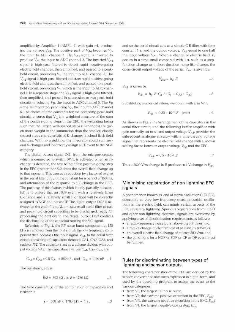
amplified by Amplifier 1 (AMPL. 1) with gain ×4, produc-ing the voltage VA4. The positive part of VA4 becomes VP, the input to ADC channel 1. The VA4 signal is inverted to produce VN, the input to ADC channel 2. The inverted VA4 signal is high-pass filtered to detect rapid negative-going electric field changes, then amplified, and passed to a peak-hold circuit, producing V4, the input to ADC channel 3. The VA4 signal is high-pass filtered to detect rapid positive-going electric field changes, then amplified, and passed to a peak-hold circuit, producing V1, which is the input to ADC chan-nel 4. In a separate stage, the VA4 signal is high-pass filtered, then amplified, and passed in succession to two peak-hold circuits, producing VB, the input to ADC channel 5. The VB signal is integrated, producing VC, the input to ADC channel 6. The choice of time constants for the preceding peak-hold circuits ensures that VC is a weighted measure of the sum of the positive-going steps in the EFC, the weighting being such that the larger, well-spaced steps (R-changes) are giv-en more weight in the summation than the smaller, closely spaced steps characteristic of K-changes in cloud flash field changes. With no weighting, the integrator could sum sev-eral K-changes and incorrectly assign a CF event to the NGF category. The digital output signal DG1 from the microprocessor, which is connected to switch SW3, is activated when an R-change is detected; the test being a fast positive-going step in the EFC greater than 0.2 times the overall field change up to that moment. This causes a reduction by a factor of twelve in the aerial filter circuit time constant for a period of 150 ms, and attenuation of the response to a C-change in the EFC. The purpose of this feature (which is only partially success-ful) is to ensure that an NGF event with a relatively large C-change and a relatively small R-change will be correctly assigned as NGF and not as CF. The digital output DG2 is ac-tivated at the end of Loop 2, and causes all aerial filter circuit and peak-hold circuit capacitors to be discharged, ready for processing the next event. The digital output DG3 controls the discharging of the capacitor storing the VC signal. Referring to Fig. 2, the RF noise burst component at 150 kHz is removed from the total signal: the low frequency com-ponent then becomes the input signal, VA1, to the aerial filter circuit consisting of capacitors denoted CA1, CA2, CA3, and resistor R/2. The capacitors act as a voltage divider, with out-put voltage VA2. The capacitance values CA1, CA2, CA3, are

CA2 = CA3 = 0.5 CA1 = 560 nF , and CA1 = 1120 nF ...1

The resistance, R/2 is

R/2 = 892 kΩ , so R = 1786 kΩ ...2

The time constant (τ) of the combination of capacitors and resistor is

τ = 560 nF × 1786 kΩ ≈ 1 s , ...3

and so the aerial circuit acts as a simple C R filter with time constant 1 s, and the output voltage, VA2 equal to one half the input voltage VA1. When a change of electric field, E, occurs in a time small compared with 1 s, such as a step-function change or a short-duration ramp-like change, the open-circuit output voltage of the aerial, Vaoc is given by:

Vaoc = ha E ...4

VA1 is given by:

VA1 = ha E Ca / (Ca + CA2 + CA3) ...5

Substituting numerical values, we obtain with E in V/m,

VA1 ≈ 0.25 × 10-3 E (volt) ...6

As shown in Fig. 2 the arrangement of the capacitors in the aerial filter circuit, and the following buffer amplifier with gain normally set to ×4 and output voltage VA4, provides the subsequent analogue circuitry with a time-varying voltage signal that represents the electric field change with a known scaling factor between output voltage VA4 and the EFC.

VA4 ≈ 0.5 × 10-3 E. ...7

Thus a 2000 V/m change in E produces a 1 V change in VA4.

Minimising registration of non-lightning EFC signals

A phenomenon known as ‘end of storm oscillations’ (EOSO), detectable as very low-frequency quasi-sinusoidal oscilla-tions in the electric field, can mimic certain aspects of the EFC caused by lightning. Spurious registrations from EOSO and other non-lightning electrical signals are overcome by applying a set of discrimination requirements as follows:• a radio-frequency noise burst above the RF threshold;• a rate of change of electric field of at least 2.5 (kV/m)/s;• an overall electric field change of at least 280 V/m; and• the conditions for a NGF or PGF or CF or DF event must

be fulfilled.

Rules for discriminating between types of lightning and sensor outputs

The following characteristics of the EFC are derived by the sensor, converted to measures expressed in digital form, and used by the operating program to assign the event to the various categories:• from V3, the largest RF noise burst;• from VP, the extreme positive excursion in the EFC, Epm;• from VN, the extreme negative excursion in the EFC, Enm;• from V4, the largest negative-going step, Ens;


• from V1, the largest positive-going step, Eps, (largest R-change);

• from VB, another measure of the positive-going steps using different time constants than those used to obtain Eps,; and

• from VC, a weighted measure of the sum of the positive-going steps, Esps.

The values of the electric field, the rate of change of field, and the overall electric field change, Eo, are obtained from VP and VN during each sampling period which is about 1.8 ms long. The discrimination tests between the various types of lightning are based on the following rules, implemented by the operating program, which have been shown by trial and error to minimise classification errors. The tests are applied in the indicated order, and, once the flash type identification has been made, the appropriate flash count register(s) is/are incremented, and the appropriate signals are sent to the AWS, as seen in the flow chart in Fig. 4.(a) Test for RF noise burst. If above threshold, other tests can

be applied.(b) Test for overall field change, Eo ≥ 280 V/m; if so, tests for

NGF, CF, and PGF can be applied. (c) Test for NGF: [Eps ≥ 0.1 Eo, or Esps ≥ 0.14 Eo] and Eo ≥

threshold for NGF.(d) Test for CF: Eps < 0.1 Eo, and Esps < 0.14 Eo, and Ens

< 0.1 Eo, and rate of change of field ≥ 2.5 (kV/m)/s, and Eo ≥ threshold for CF.

(e) Test for PGF: Ens ≥ 0.1 Eo, and Eo ≥ threshold for PGF.(f) Test for TFIR (total flash intermediate range): if tests for

NGF and CF and PGF failed, increment TFIR register.(g) Test for OL (overload condition): Epm ≥ 8 kV/m, or Enm ≥ 8

kV/m (in addition to incrementing NGF or PGF or CF and TF registers).

(h) Test for DF: if RF noise burst is above threshold, and event is not NGF or PGF or CF, increment DF register, (may be in addition to incrementing TFIR register).

(i) Test for TF (total flashes): if event is NGF or PGF or CF, increment TF register.

TFIR events are a subset of DF events that occur in an annulus just beyond the central area in which events are counted as TF; the main purpose is in checking the opera-tion of the sensor. Early versions of the sensor used 400 V/m as the common threshold for NGF, PGF and CF. As shown below, later versions used higher thresholds, and separate thresholds for NGF, PGF and CF to obtain a single lower ef-fective range for all flash types. Incorrect flash type assignment may occur as a result of limitations in the method of sensor discrimination between the three types of lightning. Six types of incorrect flash type assignment are possible, and estimates of the consequential error rates are as shown in Table 1. A cloud flash may be incorrectly assigned as NGF due to a positive-going K-change > 0.1 of overall field change, or may be incorrectly assigned as PGF due to a negative-going

K-change > 0.1 of overall field change. A negative ground flash incorrectly assigned as PGF is considered unlikely, or may be incorrectly assigned as CF: this occurs in nega-tive ground flashes with relatively large C-changes and relatively small R-changes. This problem has been partly overcome by two design features in the sensor. A positive ground flash incorrectly assigned as NGF is considered un-likely, but may be incorrectly assigned as CF due a fast neg-ative-going field change < 0.1 of overall field change. The error rate is unlikely to affect CF counts significantly, but could affect PGF counts up to about ten per cent. Indirect

Fig. 4 Flow chart for determining CGR4 output(s) to send to AWS.

Table 1. Estimated percentage rates of incorrect flash type as-signment.

Actual type of Signalled Signalled Signalledlightning as NGF as PGF as CF Negativeground flash ≤ 1% 10 - 20%

Positiveground flash ≤ 1% ≤ 1%

Cloud flash 5-10 % ≤ 1%


evidence for a low rate for incorrect assignment of NGF or CF as PGF is provided by the observation of many storms with no PGF counts, but many tens of NGF and CF counts accumulated over several storm records. For example, in a severe storm on 6 January 2006, between 1900 and mid-night (EST), a prototype CGR4 sensor in Brisbane recorded 375 NGF, 0 PGF, and 435 CF, a total of 810 events.

The performance curve and effective range of a lightning sensor

The performance curve of a lightning sensor is the rela-tionship between the fraction, f(r), of flashes counted at the range, r, and r. Normally, f(r) = 1 when r = 0, and f(r) = 0 when r ≥ Rmax, the maximum range for detection of light-ning, and for a large number of flashes there is a smooth transition of f(r) between these limits. It would be unreal-istic to expect that the sensor would count all flashes up to a particular range and none beyond, because the physical characteristics used to describe lightning, such as charges, currents, positions and dimensions of discharge chan-nels, and so on, are distributed over wide ranges of values. However, when there is insufficient information, a discon-tinuous curve based on a set of single-range estimates, has to be used. The effective range, Reff, has the value such that the num-ber of events not counted by the sensor within the range Reff is exactly balanced by the number that are counted be-yond the range Reff (Brunt and Mackerras 1961; Prentice and Mackerras 1969; Prentice 1974), where it is also shown that, given sufficient information on the relationship between f(r) and r,

K = 2 π N ∫ f(r) r dr = N π Reff2 ...8

Hence Reff = [ 2 ∫ f(r) r dr ]0.5 ...9

However, when there is insufficient information to use these equations, an approximation to the effective range can be obtained as follows. For a discontinuous performance curve f(r), the total sensor counts (K, yr-1) in an area with flash den-sity N (km-2 yr-1) is

K = ∑ N 2πr Δr f(r) …10

Also, K = N π Reff2 …11

So, Reff = √(K / N π) = √( 2∑ (r Δr f(r))), ...12

and N = K / π Reff2 ...13

With the type of lightning sensor considered here, there will be separate annual counts for NGF, PGF and CF, and sepa-rate flash density values.

Method for obtaining a single range estimate for the CGR4

The direct method for determining effective range involves observing the positions of lightning flashes in relation to the sensor position and recording whether the sensor detected the event, so as to determine values of f(r)at several values of r, e.g., using trained observers (Prentice and Mackerras 1969), or a lightning location system (LLS) (Darveniza and Uman 1984). These methods have limitations, including (a) observers very often record flashes as unidentified, (b) early LLS could only record GF, and (c) modern LLS, (e.g. http://www.vaisala.com/weather/products/ls7001.html, http://www.toasystems.com/sensors.html) normally do not identify CF. Further, it is an ob-jective for the CGR4 to apply different threshold sensitivities for NGF, PGF and CF so that the effective range is the same for all three. So, a part-theoretical part-field data method was developed to determine the relation between effective range and threshold electric field change. To calculate the field change at a distant sensor, the flash is represented by the destruction of a simple dipole, con-sisting, for a CF, of a charge +q at height h1, horizontal dis-tance x1 and direct distance d1, and a charge -q at height h2, horizontal distance x2 and direct distance d2 from the sen-sor, whereas for a GF there is only +q (or –q) with the lower charge at ground level. The discharge channel is assigned a length lo, a mid-point height hm and an angle to the vertical, θ. The method uses various plausible combinations of values of hm, lo and θ, with different values for CF and GF. This method simplifies the charge disposition and dis-charge channel geometry in real flashes, and assumes that for cloud flashes close to the sensor, the electrostatic com-ponent of the electric field change, E, (V/m) caused by the destruction of the dipole is given by Eqn 14 (adapted from Uman (1987)); for GF, h2 is zero.

E = ( 2 q / (4 π ε0) ) (h1 / d13 - h2 / d2

3) ...14

This method of obtaining single range estimates used field observations and recordings in Brisbane of the electric field changes caused by lightning, the response of a proto-type sensor, and observation of the time to thunder. An es-timate of the distance from the sensor to the middle of the discharge channel, dm, was based on the time interval be-tween the flash and the middle of the main thunder signal. Events were selected on the following bases. The identity of the event (NGF, PGF or CF) as deduced by inspection of a satisfactory electric field change (EFC) record had to agree with the identity signalled by the sensor and a satisfactory record of VA4 versus time should have been obtained, where VA4 is the internal voltage signal in the sensor that is a scaled representation of the EFC. From this information, or by di-rect measurement, the overall change in electric field, Eo, (V/m) for the event was obtained. A threshold value of overall electric field change, Et, (V/m) was selected. For the particular sensor used in these observa-


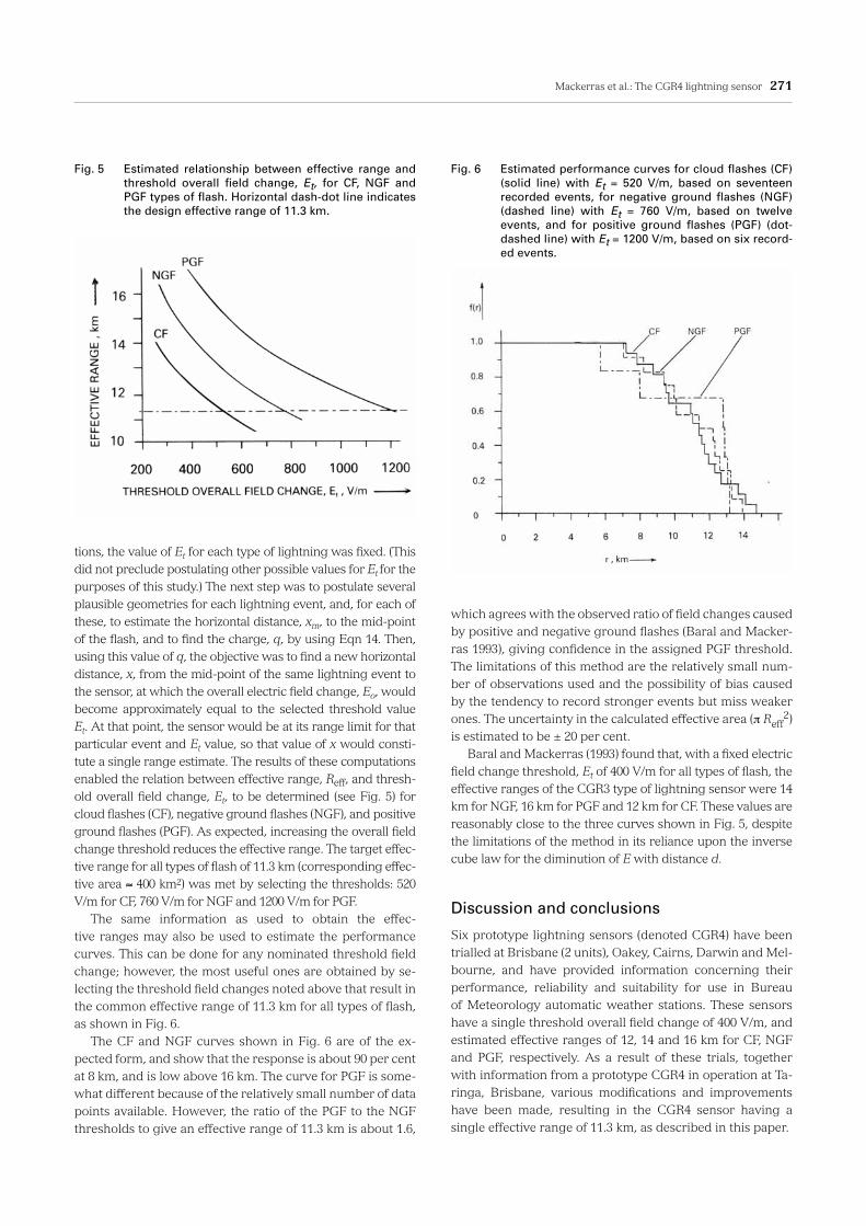
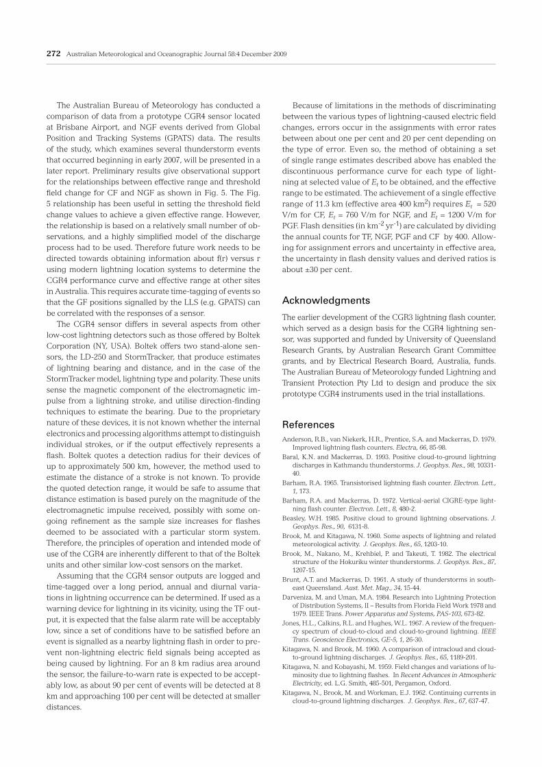
tions, the value of Et for each type of lightning was fixed. (This did not preclude postulating other possible values for Et for the purposes of this study.) The next step was to postulate several plausible geometries for each lightning event, and, for each of these, to estimate the horizontal distance, xm, to the mid-point of the flash, and to find the charge, q, by using Eqn 14. Then, using this value of q, the objective was to find a new horizontal distance, x, from the mid-point of the same lightning event to the sensor, at which the overall electric field change, Eo, would become approximately equal to the selected threshold value Et. At that point, the sensor would be at its range limit for that particular event and Et value, so that value of x would consti-tute a single range estimate. The results of these computations enabled the relation between effective range, Reff, and thresh-old overall field change, Et, to be determined (see Fig. 5) for cloud flashes (CF), negative ground flashes (NGF), and positive ground flashes (PGF). As expected, increasing the overall field change threshold reduces the effective range. The target effec-tive range for all types of flash of 11.3 km (corresponding effec-tive area ≈ 400 km2) was met by selecting the thresholds: 520 V/m for CF, 760 V/m for NGF and 1200 V/m for PGF. The same information as used to obtain the effec-tive ranges may also be used to estimate the performance curves. This can be done for any nominated threshold field change; however, the most useful ones are obtained by se-lecting the threshold field changes noted above that result in the common effective range of 11.3 km for all types of flash, as shown in Fig. 6. The CF and NGF curves shown in Fig. 6 are of the ex-pected form, and show that the response is about 90 per cent at 8 km, and is low above 16 km. The curve for PGF is some-what different because of the relatively small number of data points available. However, the ratio of the PGF to the NGF thresholds to give an effective range of 11.3 km is about 1.6,

which agrees with the observed ratio of field changes caused by positive and negative ground flashes (Baral and Macker-ras 1993), giving confidence in the assigned PGF threshold. The limitations of this method are the relatively small num-ber of observations used and the possibility of bias caused by the tendency to record stronger events but miss weaker ones. The uncertainty in the calculated effective area (π Reff

2) is estimated to be ± 20 per cent. Baral and Mackerras (1993) found that, with a fixed electric field change threshold, Et of 400 V/m for all types of flash, the effective ranges of the CGR3 type of lightning sensor were 14 km for NGF, 16 km for PGF and 12 km for CF. These values are reasonably close to the three curves shown in Fig. 5, despite the limitations of the method in its reliance upon the inverse cube law for the diminution of E with distance d.

Discussion and conclusions

Six prototype lightning sensors (denoted CGR4) have been trialled at Brisbane (2 units), Oakey, Cairns, Darwin and Mel-bourne, and have provided information concerning their performance, reliability and suitability for use in Bureau of Meteorology automatic weather stations. These sensors have a single threshold overall field change of 400 V/m, and estimated effective ranges of 12, 14 and 16 km for CF, NGF and PGF, respectively. As a result of these trials, together with information from a prototype CGR4 in operation at Ta-ringa, Brisbane, various modifications and improvements have been made, resulting in the CGR4 sensor having a single effective range of 11.3 km, as described in this paper.

Fig. 5 Estimated relationship between effective range and threshold overall field change, Et, for CF, NGF and PGF types of flash. Horizontal dash-dot line indicates the design effective range of 11.3 km.

Fig. 6 Estimated performance curves for cloud flashes (CF) (solid line) with Et = 520 V/m, based on seventeen recorded events, for negative ground flashes (NGF) (dashed line) with Et = 760 V/m, based on twelve events, and for positive ground flashes (PGF) (dot-dashed line) with Et = 1200 V/m, based on six record-ed events.


Because of limitations in the methods of discriminating between the various types of lightning-caused electric field changes, errors occur in the assignments with error rates between about one per cent and 20 per cent depending on the type of error. Even so, the method of obtaining a set of single range estimates described above has enabled the discontinuous performance curve for each type of light-ning at selected value of Et to be obtained, and the effective range to be estimated. The achievement of a single effective range of 11.3 km (effective area 400 km2) requires Et = 520 V/m for CF, Et = 760 V/m for NGF, and Et = 1200 V/m for PGF. Flash densities (in km-2 yr-1) are calculated by dividing the annual counts for TF, NGF, PGF and CF by 400. Allow-ing for assignment errors and uncertainty in effective area, the uncertainty in flash density values and derived ratios is about ±30 per cent.

Acknowledgments

The earlier development of the CGR3 lightning flash counter, which served as a design basis for the CGR4 lightning sen-sor, was supported and funded by University of Queensland Research Grants, by Australian Research Grant Committee grants, and by Electrical Research Board, Australia, funds. The Australian Bureau of Meteorology funded Lightning and Transient Protection Pty Ltd to design and produce the six prototype CGR4 instruments used in the trial installations.

References Anderson, R.B., van Niekerk, H.R., Prentice, S.A. and Mackerras, D. 1979.

Improved lightning flash counters. Electra, 66, 85-98.Baral, K.N. and Mackerras, D. 1993. Positive cloud-to-ground lightning

discharges in Kathmandu thunderstorms. J. Geophys. Res., 98, 10331-40.

Barham, R.A. 1965. Transistorised lightning flash counter. Electron. Lett., 1, 173.

Barham, R.A. and Mackerras, D. 1972. Vertical-aerial CIGRE-type light-ning flash counter. Electron. Lett., 8, 480-2.

Beasley, W.H. 1985. Positive cloud to ground lightning observations. J. Geophys. Res., 90, 6131-8.

Brook, M. and Kitagawa, N. 1960. Some aspects of lightning and related meteorological activity. J. Geophys. Res., 65, 1203-10.

Brook, M., Nakano, M., Krehbiel, P. and Takeuti, T. 1982. The electrical structure of the Hokuriku winter thunderstorms. J. Geophys. Res., 87, 1207-15.

Brunt, A.T. and Mackerras, D. 1961. A study of thunderstorms in south-east Queensland. Aust. Met. Mag., 34, 15-44.

Darveniza, M. and Uman, M.A. 1984. Research into Lightning Protection of Distribution Systems, II – Results from Florida Field Work 1978 and 1979. IEEE Trans. Power Apparatus and Systems, PAS-103, 673-82.

Jones, H.L., Calkins, R.L. and Hughes, W.L. 1967. A review of the frequen-cy spectrum of cloud-to-cloud and cloud-to-ground lightning. IEEE Trans. Geoscience Electronics, GE-5, 1, 26-30.

Kitagawa, N. and Brook, M. 1960. A comparison of intracloud and cloud-to-ground lightning discharges. J. Geophys. Res., 65, 1189-201.

Kitagawa, N. and Kobayashi, M. 1959. Field changes and variations of lu-minosity due to lightning flashes. In Recent Advances in Atmospheric Electricity, ed. L.G. Smith, 485-501, Pergamon, Oxford.

Kitagawa, N., Brook, M. and Workman, E.J. 1962. Continuing currents in cloud-to-ground lightning discharges. J. Geophys. Res., 67, 637-47.

The Australian Bureau of Meteorology has conducted a comparison of data from a prototype CGR4 sensor located at Brisbane Airport, and NGF events derived from Global Position and Tracking Systems (GPATS) data. The results of the study, which examines several thunderstorm events that occurred beginning in early 2007, will be presented in a later report. Preliminary results give observational support for the relationships between effective range and threshold field change for CF and NGF as shown in Fig. 5. The Fig. 5 relationship has been useful in setting the threshold field change values to achieve a given effective range. However, the relationship is based on a relatively small number of ob-servations, and a highly simplified model of the discharge process had to be used. Therefore future work needs to be directed towards obtaining information about f(r) versus r using modern lightning location systems to determine the CGR4 performance curve and effective range at other sites in Australia. This requires accurate time-tagging of events so that the GF positions signalled by the LLS (e.g. GPATS) can be correlated with the responses of a sensor. The CGR4 sensor differs in several aspects from other low-cost lightning detectors such as those offered by Boltek Corporation (NY, USA). Boltek offers two stand-alone sen-sors, the LD-250 and StormTracker, that produce estimates of lightning bearing and distance, and in the case of the StormTracker model, lightning type and polarity. These units sense the magnetic component of the electromagnetic im-pulse from a lightning stroke, and utilise direction-finding techniques to estimate the bearing. Due to the proprietary nature of these devices, it is not known whether the internal electronics and processing algorithms attempt to distinguish individual strokes, or if the output effectively represents a flash. Boltek quotes a detection radius for their devices of up to approximately 500 km, however, the method used to estimate the distance of a stroke is not known. To provide the quoted detection range, it would be safe to assume that distance estimation is based purely on the magnitude of the electromagnetic impulse received, possibly with some on-going refinement as the sample size increases for flashes deemed to be associated with a particular storm system. Therefore, the principles of operation and intended mode of use of the CGR4 are inherently different to that of the Boltek units and other similar low-cost sensors on the market. Assuming that the CGR4 sensor outputs are logged and time-tagged over a long period, annual and diurnal varia-tions in lightning occurrence can be determined. If used as a warning device for lightning in its vicinity, using the TF out-put, it is expected that the false alarm rate will be acceptably low, since a set of conditions have to be satisfied before an event is signalled as a nearby lightning flash in order to pre-vent non-lightning electric field signals being accepted as being caused by lightning. For an 8 km radius area around the sensor, the failure-to-warn rate is expected to be accept-ably low, as about 90 per cent of events will be detected at 8 km and approaching 100 per cent will be detected at smaller distances.


Kuleshov, Y. and Jayaratne, E.R. 2004. Estimates of lightning ground flash density in Australia and its relationship to thunder-days. Aust. Met. Mag., 53, 186-96.

Mackerras, D. 1968. A comparison of discharge processes in cloud and ground lightning flashes. J. Geophys. Res., 73, 1175-83.

Mackerras, D. 1985. Automatic short range measurement of the cloud flash to ground flash ratio in thunderstorms. J. Geophys. Res., 90, 6195 201.

Ogawa, T. and Brook, M. 1969. Charge distribution in thunderstorm clouds. Q. Jl R. Met. Soc., 95, 513-25.

Prentice, S.A. 1974. The CIGRE lightning flash counter: Australian experi-ence. Int. Conf. Large High Voltage Electric Systems, Working Group 33-04, 1974.

Prentice, S.A. and Mackerras, D. 1969. Recording range of a lightning flash counter. Proc. Inst. Elec. Eng., 116, 294-302.

Prentice, S.A., Mackerras, D. and Tolmie R.P. 1975. Development and field testing of a vertical-aerial lightning-flash counter. Proc. Inst. Elec. Eng., 122, 487-91.

Rakov, V.A. and Uman, M.A. 2003. Lightning: Physics and Effects, Cam-bridge University Press.

Shao, X.M., Rhodes, C.T. and Holden, D.N. 1999. RF radiation observations of positive cloud-to-ground flashes. J. Geophys. Res., 104, 9601-8.

Takeuti, T., Nakano, M. and Yamamoto, Y. 1976. Remarkable characteris-tics of cloud to ground discharges observed in winter thunderstorms in Hokuriku area, Japan. J. Met. Soc. Japan, 54, 436-40.

Thomson, E.M. 1980. Characteristics of Port Moresby ground flashes. J. Geophys. Res., 85, 1027-36.

Thottappillil, R., Rakov, V.A. and Uman, M.A. 1990. K and M changes in close lightning ground flashes in Florida. J. Geophys. Res., 95, 18631-40.

Uman, M.A. 1987. The Lightning Discharge. Academic Press, Orlando, Florida.


Documents

The CGR4 lightning sensor - Bureau of Meteorology · 2010-03-09 · the lightning flash and the fraction of flashes counted at that distance is a feature of the sensor known as its