Embed Size (px)
Citation preview

The CGMS Statistical Tool
User Manual v 3.0
Paul W. Goedhart1, Steven B. Hoek2 and Hendrik L. Boogaard2
March 2017
1 Wageningen University and Research, Wageningen Plant Research (Biometris), the Netherlands 2 Wageningen University and Research, Wageningen Environmental Research (Alterra), the Netherlands

CGMS Statistical Tool 2
Mission of the JRC As the Commission's in-house science service, the Joint Research Centre's mission is to provide EU policies with independent, evidence-based scientific and technical support throughout the whole policy cycle. Working in close cooperation with policy Directorates-General, the JRC addresses key societal challenges while stimulating innovation through developing new methods, tools and standards, and sharing its know-how with the Member States, the scientific community and international partners. European Commission Joint Research Centre (JRC) Sustainable Resources Directorate (SRD) Monitoring Agricultural Resources Unit (MARS) 21027 Ispra (VA) Italy E-mail: [email protected] Website: http://mars.jrc.ec.europa.eu Legal Notice: Neither the European Commission nor any person on behalf of the Commission is responsible for the use that might be made of the information contained in this production. © European Commission, 2017 Reproduction is authorised provided the source is acknowledged.

The CGMS Statistical Tool User Manual v 3.0 Paul W. Goedhart, Steven B. Hoek and Hendrik L. Boogaard
Wageningen University and Research, Wageningen, 2017

CGMS Statistical Tool 4
ABSTRACT Paul W. Goedhart, Steven B. Hoek and Hendrik L. Boogaard, 2017. The CGMS Statistical Tool. User Manual – v 3.0, Wageningen University and Research, Wageningen, 105 pp. The CGMS statistical tool has been developed for the MARS unit of JRC in the framework of the several MARS projects (MARSOP, ASEMARS, E-Agri, AGRICAB and SIGMA). These projects were all meant to further improve the MARS Crop Yield Forecasting System (MCYFS). The tool is designed to support the development and selection of crop yield forecast models to facilitate national and sub national crop yield forecasting. Time trend analysis of yield statistics is followed by regression or scenario analysis using biophysical indicators to explain yield statistics and search for similar years. Constructed models are used to predict yield of the current growing season. Keywords: CGMS, MCYFS, crop yield forecast, crop yield statistics

CGMS Statistical Tool
Contents
Preface 9
Summary 11
1 Introduction 13
1.1 The CGMS Statistical Tool in the context of the MARS Project 13
1.2 The improvement of the statistical module of CGMS in ASEMARS 14
1.3 Guide for reading this manual 14
2 Overview of interface and functionality 16
3 Selecting an area, crop and period (dekad) 18
3.1 Area 18
3.2 Crop 18
3.3 Period (dekad) 18
3.4 Retrieve analyst settings 19
4 Data analysis and time trend analysis 22
4.1 Selection of years 22
4.2 Detection of outliers 24
4.3 Selection of the appropriate time trend 27
4.4 Testing the trend 29
4.5 Analysing the trend model 29
5 Indicators page: selecting indicators to include 30
5.1 Regression analysis 30 5.1.1 Forecast mode 30 5.1.2 Calibration mode 32
5.2 Scenario analysis 33
6 Options page: setting options for output 35
7 Output page: viewing the results 38
7.1 Regression Models 38
7.2 Scenario models 39
7.3 Saving model 41
7.4 Export settings 42

CGMS Statistical Tool 6
8 Model details page: viewing results of a selected model 43
8.1 Regression 43 8.1.1 Description of regression model 43 8.1.2 Summary Statistics 43 8.1.3 Regression coefficients 44 8.1.4 Confidence intervals for prediction 44 8.1.5 Case statistics 44 8.1.6 Plots for diagnosing the model 45
8.2 Scenario analysis 46 8.2.1 Description of scenario model 46 8.2.2 Time trend coefficients 46 8.2.3 Principal Component Analysis - parameters 46 8.2.4 Explained variance 46 8.2.5 Principal Component Analysis - loadings 46 8.2.6 Clustering of years 47 8.2.7 Overview of residuals relative to the trend 47 8.2.8 Summary Statistics 47 8.2.9 Prediction 47 8.2.10 Case statistics 48 8.2.11 Plots for diagnosing the model 48
9 Saved Models 49
10 Some Statistical Issues 51
10.1 Selection of the Best Model 51
10.2 The best subset model may not always be the best 53
10.3 Multicollinearity and Variance Inflation Factors 53
10.4 Regression Diagnostics and Case Statistics 54
10.5 Perfect Fit and Aliasing of indicators 56
10.6 Comments on scenario analysis 57
11 Installation, databases and file menu 58
11.1 Installation 58
11.2 Database structure 59
11.3 Filling the database 61
11.4 File menu 62 11.4.1 File – change database 62 11.4.2 File – managing settings 63 11.4.3 File – miscellaneous 64 11.4.4 View 64 11.4.5 Tools 65 11.4.6 Help 65

CGMS Statistical Tool
12 Analyst settings and batch mode 66
12.1 Analyst settings 66 12.1.1 Format 66 12.1.2 Where do settings come from? 66 12.1.3 How to retrieve settings? 67
12.2 Batch mode 68 12.2.1 Best model selected 68 12.2.2 Minimum number of years 69 12.2.3 Batch processing via interactive mode 69 12.2.4 Command line 71 12.2.5 Process all best subset models 72
13 Data import and management 74
13.1 Import RUM 75
13.2 Accumulate data (fixed start dekad and a moving end dekad) 77
13.3 Copy data 78
13.4 Accumulate data (fixed period, moving start and end dekad) 80
14 References 82
Annex 1 Structure of the database 83
Annex 2 How to configure the tool for another database 89
Annex 3 Analyst settings 91
Annex 4 Configuration options 95
Annex 5 Acronyms and abbreviations 98
Annex 6 How to prepare your data for analysis 102


CGMS-Statistical-Tool_V_3_0.docxCGMS Statistical Tool 9
Preface
The CGMS statistical tool has been developed for the MARS unit of JRC in the framework of several MARS related projects (MARSOP, ASEMARS, E-Agri, AGRICAB and SIGMA). These projects were all meant to further improve the MARS Crop Yield Forecasting System (MCYFS). The work was carried out by two institutes of the Wageningen University and Research: Wageningen Environmental Research (Alterra) and Wageningen Plant Research (Biometris). The tool is designed to support the development and selection of crop yield forecast models to facilitate national and sub national crop yield forecasting. The authors would like to thank Giampiero Genovese, Manola Bettio, Bettina Baruth, Davide Fanchini, Iacopo Cerrani, Olivier Leo, Felix Rembold and Hervé Kerdiles of the MARS unit of the Joint Research Centre for very fruitful discussions. We would like to also acknowledge the constructive comments we received from Riad Balaghi of INRA Morocco. We are indebted to Yannick Curnel and Roger Oger of the Walloon Agricultural Research Centre for a very thorough and detailed validation of a beta version of CgmsStatTool. Curnel and Oger (2006) thoroughly tested and validated a beta version of CgmsStatTool, which contained only features relevant for regression analysis. The output of the Fortran subroutines TIMETREND, CORRELATION, FITMODEL, SINGLE and BESTSUBSET was compared with the output of the statistical program GenStat (2005). This was done for a variety of datasets. We would also like to thank Allard de Wit and Kees van Diepen of Alterra for their cooperation.


CGMS Statistical Tool 11
Summary
The CGMS statistical tool has been developed for the MARS unit of JRC in the framework of several MARS related projects (MARSOP, ASEMARS, E-Agri, AGRICAB and SIGMA). These projects contributed to development of the initial version and a number of subsequent updates. The original objective was to support the national crop yield forecasting activities of the MARS Crop Yield Forecasting System (MCYFS). Later, through EU research project like E-Agri, AGRICAB and SIGMA the CGMS statistical tool has been introduced to other (non)-governmental organizations having a mandate in monitoring and forecasting crop production. The tool is designed to support the development and selection of crop yield forecast models to facilitate national and sub national crop yield forecasting. Time trend analysis of yield statistics is followed by regression or scenario analysis using biophysical indicators to explain yield statistics and search for similar years. Constructed models are used to predict yield of the current growing season Recent extensions of the tool include support to ease the work needed beforehand to fill the database with indicator data. The tool has functions to manage indicator data such as the import of SPIRITS RUM files, the aggregation of dekadal data over flexible periods and the mapping of certain dekad specific indicators to a range of dekads. Another important feature is to run the tool in batch for testing models for a range of dekads or to embed the tool in an operational production line. This report describes the latest version of the statistical tool, which will be called CGMS Statistical Tool or CgmsStatTool for short in the following. The interface was developed using Delphi as programming language. Part of the underlying statistical functionality was however partially developed in Fortran as the programming language so that we could benefit from the high quality routines of the IMSL Fortran library. That library is invoked respectively for fitting single and multiple regression models. This report is not intended as an introduction to the statistical principles underlying both regression and scenario analysis. It is therefore assumed that users of CgmsStatTool have a certain understanding of the basic principles of linear regression and principal component analysis. Before using the tool in an operational way, the user is strongly advised to play with the tool and to read the chapter “Some Statistical Issues”. An excellent and complete introduction into linear regression is the book by Montgomery, Peck and Vining (2001). Suggestions for further readings on principal component analysis are provided in the reference section. Chapters 2-9 of this report describe the CgmsStatTool interface and purpose in detail. Chapter 10 contains important remarks on several statistical issues related to proper use of the tool. Chapters 11 and 12 describe technical aspects like the installation, the databases used by the program, the way in which analyst settings can be saved, copied, modified and shared, a description of the menu items and the batch mode.

CGMS Statistical Tool 12
Functionality around indicator data management is described in Chapter 13. References are listed in Chapter 14. In the annexes a detailed description is given of the database and of the user settings. More on the statistical procedures covered in this manual and their application to crop forecasting can be found in the Mars Crop Yield Forecasting System (MCYFS) wiki: http://marswiki.jrc.ec.europa.eu/agri4castwiki/index.php/Main_Page Reference should be made especially to the following sections: http://marswiki.jrc.ec.europa.eu/agri4castwiki/index.php/Yield_Forecasting http://marswiki.jrc.ec.europa.eu/agri4castwiki/index.php/Forecasting_methods.

CGMS Statistical Tool 13
1 Introduction
1.1 The CGMS Statistical Tool in the context of the MARS Project
The CGMS statistical tool has been developed for the MARS unit of JRC in the framework of several MARS related projects such as MARSOP, ASEMARS, E-Agri, AGRICAB and SIGMA. These projects were all meant to further improve the MARS Crop Yield Forecasting System (MCYFS). The work was carried out by two institutes of the Wageningen University and Research: Wageningen Environmental Research (Alterra) and Wageningen Plant Research (Biometris). The tool is designed to support the development and selection of crop yield forecast models to facilitate national and sub national crop yield forecasting. The MARS project, for “Monitoring Agriculture with Remote Sensing” started in 1988 and was initially designed to provide to the DG Agriculture and DG EUROSTAT, independent and timely information on crop areas and yields. Since 1993 this information is brought together in the MARS Bulletin with early crop forecasts during the campaign till the obtaining of the official EU statistics. The interest of this activity is to provide every month, independently of Member States, real-time information on productions expected and to identify regional anomalies. MARS Bulletin is based on analysis of meteorological conditions, of results of crop growth simulation models using meteorological observations and high temporal resolution satellite data (VEGETATION or NOAA/AVHRR). It concerns European Union, Candidate Countries, Eastern European countries and Maghreb. Since 2001, the MARS Bulletin outputs are used as official crop forecasts by DG Agriculture and are integrated in the EUROSTAT crop forecast system. The analytical procedures start with screening and statistical analyses of data produced in the MCYFS and this forms the basis for crop yield forecasting at national and European level. The agro-meteorological model used within the MCYFS in MARS is the CGMS (Crop Growth Monitoring System). The core of the model for crop growth simulation consists in an adaptation of the WOFOST model (see http://www.wageningenur.nl/wofost). The crop simulation model WOFOST calculates, among other model outputs, potential yield and potential total biomass as a function of weather and soil conditions. The WOFOST model integrates all the effects of the varying weather conditions which give different potential yields over the years. The model output is aggregated from single land units to administrative regions. In 1992 and 1993 it was studied whether regionally aggregated output of the WOFOST crop model could be used for regional crop yield forecasting. This was done by regressing the official statistics of yearly yields onto the model output of WOFOST. Because the official yields frequently showed a yearly increase, a technological linear trend was added to the regression model if necessary. Since the fitted relations were adequate for prediction purposes, a statistical module for CGMS level 3 was developed. The module selected from four candidate WOFOST model outputs, further called indicators, the best performing indicator (e.g. potential total biomass or potential yield). The ‘best’ model, with a single indicator, was then used for forecasting the yield in the current year. In the operational CGMS system this was done for each crop region combination at the end of each dekad (10 day period) during the agricultural season. This first version of the statistical subsystem employed a Fortran executable. The system was rebuilt in the year 2000 to enable the use of a

CGMS Statistical Tool 14
Fortran DLL within S PLUS. The Fortran DLL that selects and calculates the regression models did not change. However, S Plus did not function very well in an operational production line. Therefore in CGMS version 8.0 the selection of data and indicators was organized in the user interface of C++. A dedicated Delphi program served as a statistical engine and called the Fortran DLL for performing linear regression. 1.2 The improvement of the statistical module of CGMS in ASEMARS
The improvement of the statistical module of CGMS in ASEMARS was part of a larger research effort launched by the MARS Unit to complete and reinforce the CGMS in order to extend the system thematically and geographically in support to the operational activities, and to improve the efficacy of the system, and flexibility. The improvement of the statistical module associated to CGMS involved the extension of the functionalities of the system based on the following requirements:
• Allow to select from the data base any meteo / crop / remote sensing (RS) based parameter individually as indicator (for a maximum of 30 predefined parameters) in the regression analysis;
• The implementation of automatic multi-regressive approaches in order to let emerge the best model;
• Automatic performances check on the regression models obtained and statistical tests to take the decision on which is the best model that must be proposed as final each dekad running;
• Complete the implementation of the scenario analysis (that was already applied by MARS internally;
• And implementing the algorithm for the prediction calculations. Further improvements were implemented since the ASEMARS project which are reflected in the current version 3.0. We list here the most important ones:
• Support to ease the work needed beforehand to fill the database with indicator data and allow to work with agriculture campaigns that differs from calendar years. The tool has functions to manage indicator data such as the import of SPIRITS RUM files, the aggregation of dekadal data over flexible periods and the mapping of certain dekad specific indicators to a range of dekads;
• Feature to run the tool in batch for testing models for a range of dekads or to embed the tool in an operational production line;
• A major update of the user interaction addressing issues like switching database, outlier detection, terminology, etc.
For recent improvements of the last releases see the release notes included in the current installation. 1.3 Guide for reading this manual
This report describes the CGMS Statistical Tool or CgmsStatTool for short. The interface has been built using Delphi. For the underlying statistical functionality Fortran was still used as the

CGMS Statistical Tool 15
programming language and high quality routines of the IMSL Fortran library are being invoked, e.g. for fitting a single regression model. This report is not intended as an introduction to the statistical principles underlying both regression and scenario analysis. It is therefore assumed that users of CgmsStatTool have a firm understanding of the basic principles of linear regression and principal component analysis. Before using the tool in an operational way, the user is strongly advised to play with the tool and to read the chapter “Some Statistical Issues”. An excellent and complete introduction into linear regression is the book by Montgomery, Peck and Vining (2001). Users of CgmsStatTool are encouraged to read the following chapters of this book: 3. Multiple Linear Regression; 4. Model Adequacy Checking; 6. Diagnostics for Leverage and Influence; 9. Variable Selection and Model Building; 10. Multicollinearity. Montgomery, Peck and Vining (2001) is frequently quoted, sometimes not explicitly, and referenced in this report. References are denoted by MPV followed by the relevant page number. Suggestions for further readings on principal component analysis are provided in the reference section. Chapters 2-9 of this report describe the CgmsStatTool interface and purpose in detail. Chapter 10 contains important remarks on several statistical issues related to proper use of the tool. Chapters 11 and 12 describe technical aspects like the installation, the databases used by the program, the way in which analyst settings can be saved, identified, retrieved, copied, modified and shared, a description of the menu items and the batch mode. Functionality around indicator data management is described in Chapter 13. References are listed in Chapter 14. In the annexes a detailed description is given of the database and of the user settings.

CGMS Statistical Tool 16
2 Overview of interface and functionality
This chapter gives a brief overview of the interface and functionality of CgmsStatTool. A detailed description is given in subsequent chapters. Running CgmsStatTool in normal mode presents the user with the following opening screen.
The screen is divided into four parts:
1. A top row with a few menu items (read more in Chapter 11); 2. The left panel can be used to specify an area or region. This is done by selecting an area
(most frequently an administrative or reporting unit) from a drop-down list. Once the area is selected the available crops are shown in a second drop-down list. After selecting a crop, the user must select a period (dekad) for which a prediction must be made. By default this is the current period (read more in Chapter 3);
3. The right panel consists of the following four tab pages: • A page for Data analysis; here the yield data and the indicator data can be inspected
so that possible anomalies can be detected and excluded; • A page for Time trend analysis; this page can be used to specify the calibration period,
the target year for which the yield must be predicted, the time trend model and possibly a logarithmic transformation for year (read more in Chapter 4);

CGMS Statistical Tool 17
• A page for Regression analysis; • A page for Scenario analysis.
4. A fourth optional panel, at the bottom of the screen, can be shown by the {View | Log Window} menu item. This displays various warnings and errors that might occur, e.g. when indicators are aliased or when a perfect fit is obtained for a linear time trend model.
The user can open any of the four tab pages for analysis by using the vertical tabs which are placed on the top left just above the controls for selecting area, crop and period. It should be noted that regression and scenario analysis are always based upon time trend analysis. Therefore the user always must activate and check the time trend analysis before continuing the regression and scenario analysis.
Both, the tab page for regression analysis and the one for scenario analysis in turn consist of five tab pages which can be opened using horizontal tabs at the top:
• The Indicators page can be used to select indicators which should enter the regression model or should be used in the scenario analysis. In case of regression analysis indicators can be either free or forced. Forced indicators are included in every regression model, while free indicators are either included or excluded from a model. The correlation matrix between the selected indicators can be viewed from this page (read more in Chapter 5);
• The Options page presents the user with all options. In case of regression analysis the main choice is between the single free indicators method and the method of best subset selection. The single free indicators method fits models with only one free indicator, in addition to the chosen time trend and forced indicators, if any. The best subset selection method searches for the best models, according to some criterion, with multiple free indicators. There are various options to aid the user in selecting a proper model for prediction of the target year (read more in Chapter 6);
• The Output page displays the various, single indicator or best subset, regression models and results of the scenario analysis. Criteria for the different models are displayed as well as t values of included indicators. The t values can be coloured according to the sign or the significance of the corresponding regression coefficient. In case of scenario analysis only one criterion is presented: residual standard deviation; a choice for the best model can be made and the particulars for that model can be saved (read more in Chapter 7);
• The Model Details page is activated by clicking on a single model on the Output page. A detailed analysis of the single model is presented including a description of the model, summary statistics, regression coefficients, case statistics such as fitted values, residuals and leverages, and finally a graphical representation of the case statistics (read more in Chapter 8);
• The Saved Model page shows selected particulars of all the models that were saved for the currently selected area, crop and period – both regression and scenario models. Such models can be renamed, retrieved as well as deleted by means of the buttons on this page (read more in Chapter 9).

CGMS Statistical Tool 18
3 Selecting an area, crop and period (dekad)
3.1 Area
A country can be selected by clicking on the name in the Area list box on the left. When a country is selected, lower administrative areas for that country then appear indented below the country name. A lower administrative area can therefore only be selected after the relevant country has been selected first. The same is true for administrative areas at lower levels.
3.2 Crop
The Crop list box will be updated to show the crops for which there are data available in the selected area. Upon each selection in the left panel the Data analysis and Time trend analysis page on the right are refreshed. If no data are available for the selected area and crop, an informational message appears in the log window: “No crop statistics available for this area”. 3.3 Period (dekad)
Finally, the user has to select the period (dekad) for which the analysis should be carried out. The term dekad refers to a ten day period. A month is considered to consist of three dekads, the first taking from day 1 to day 10, the second from day 11 to day 20 and the last from day 21 to the end of the month. In the tool dekads are indicated in two ways:
- by the name of the month followed by a Roman figure: I, II or III; - by a number in the range 1 through 36.
CGMS Statistical Tool 19
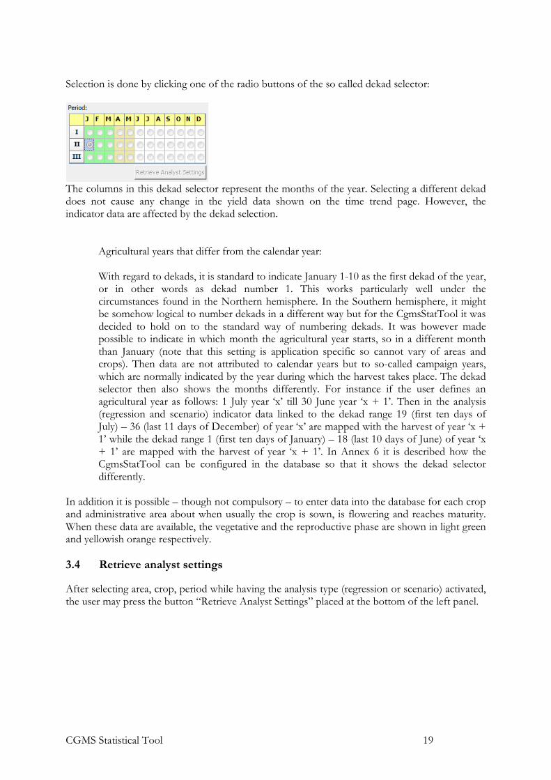
Selection is done by clicking one of the radio buttons of the so called dekad selector:
The columns in this dekad selector represent the months of the year. Selecting a different dekad does not cause any change in the yield data shown on the time trend page. However, the indicator data are affected by the dekad selection.
Agricultural years that differ from the calendar year: With regard to dekads, it is standard to indicate January 1-10 as the first dekad of the year, or in other words as dekad number 1. This works particularly well under the circumstances found in the Northern hemisphere. In the Southern hemisphere, it might be somehow logical to number dekads in a different way but for the CgmsStatTool it was decided to hold on to the standard way of numbering dekads. It was however made possible to indicate in which month the agricultural year starts, so in a different month than January (note that this setting is application specific so cannot vary of areas and crops). Then data are not attributed to calendar years but to so-called campaign years, which are normally indicated by the year during which the harvest takes place. The dekad selector then also shows the months differently. For instance if the user defines an agricultural year as follows: 1 July year ‘x’ till 30 June year ‘x + 1’. Then in the analysis (regression and scenario) indicator data linked to the dekad range 19 (first ten days of July) – 36 (last 11 days of December) of year ‘x’ are mapped with the harvest of year ‘x + 1’ while the dekad range 1 (first ten days of January) – 18 (last 10 days of June) of year ‘x + 1’ are mapped with the harvest of year ‘x + 1’. In Annex 6 it is described how the CgmsStatTool can be configured in the database so that it shows the dekad selector differently.
In addition it is possible – though not compulsory – to enter data into the database for each crop and administrative area about when usually the crop is sown, is flowering and reaches maturity. When these data are available, the vegetative and the reproductive phase are shown in light green and yellowish orange respectively. 3.4 Retrieve analyst settings
After selecting area, crop, period while having the analysis type (regression or scenario) activated, the user may press the button “Retrieve Analyst Settings” placed at the bottom of the left panel.

CGMS Statistical Tool 20
The following settings view is opened:
The form has two tab sheets for retrieving settings: for file-based analyst settings and for analyst settings stored in the database:
• File based: this shows the available set of CST settings stored in the settings file. By default the CgmsStatTool is linked to a file called CgmsStatTool.csv. However the user can select other settings files as explained in section 11.4.2. Note that this view shows the set of CST settings that belong to the region / area and crop selected in the left panel. There can be sets for different periods (dekads) and different analysis types (regression or scenario).
• Database: this shows settings that are retrieved from a table in the database that is filled (together with a few other tables with details on the selected model) when a user saves a model to the database. There can be sets for different periods (dekads) and different analysis types (regression or scenario). In addition it is possibly to have more than one set of CST settings per combination of selected area, crop, period (dekad) and analysis type as the CgmsStatTool allows saving multiple instances for such combination to the database e.g. saving models that only differ with regard to the included indicators or the included time trend.
When the user then presses OK in this form, the selected analyst settings are applied to the user interface and the user can then quickly proceed with selecting the best model for the selected area, crop, period and analysis type. In addition there is a tab to copy settings to other dekad and / or regions. This is explained in section 12.2.3 (batch processing via interactive mode).

CGMS Statistical Tool 21
More information on analyst settings can be found in Chapter 12.

CGMS Statistical Tool 22
4 Data analysis and time trend analysis
Before the user can proceed with regression or scenario analysis, he or she is offered the chance to screen the data for possible anomalies and to establish whether the yield data contain a trend: by means of data analysis and time trend analysis respectively. Time trend analysis is not offered as an independent analysis, meaning that the user is expected to always continue with regression or scenario analysis. 4.1 Selection of years
After the area, crop and period are selected, the Data analysis page is normally active with the horizontal tab sheet “View data” open. Both the yield data and the indicator data are shown. Note that the official yields are shown for all the years for which they are available and that they are not affected by the period (dekad) selector on the left. The indicator values are however specific for dekads. In the installed sample database indicators are available for all dekads of the growing season for a selected crop. In the case of the CGMS indicators (01 to 04) the end values at maturity are stored in the database for the remaining dekads of the year after the growing season. The database does not contain CGMS indicator values for dekads preceding the dekad of sowing.

CGMS Statistical Tool 23
Years with missing official yields are always displayed in grey and missing data in the indicators are highlighted in yellow. Individual years can be excluded or included by checkboxes on the left; years which are excluded are highlighted in grey. The checkboxes for years with missing official yields are disabled and also highlighted in grey. All years with missing values in any of the columns can be excluded by employing the “Exclude missing” button. All years, except the ones with missing official yields, can be included by using the “Reset” button. The OK button must be used to confirm the changes made, or you can press the Cancel button to leave the Data View without making any changes. The button “Full screen” allows the user to inspect and exclude the data on a window that fills the complete screen. Data can be exported through “Copy to clipboard” for instance to paste into Excel or Word file. There can be a number of reasons why one would like to exclude years. This is dealt with in paragraph 4.2. Further selection of the years is done on the time trend page. Initially, the time trend page displays the start and end year for which there are yield data in the database. If any early years were excluded, this is taken into account. The default target year, for which a prediction will be made, is the end year plus one. These values can be modified by the user. The only restriction is that there must be at least four years from start to end year. And the target year cannot be chosen more than 3 years ahead – in other words: that is the time horizon.

CGMS Statistical Tool 24
The user is informed about the time span covered by the years in the database, the number of years for which crop yield data are available in the database, and the number of excluded / missing years1. 4.2 Detection of outliers
In the Data analysis there are, in addition to the horizontal tab sheet “view data”, two other horizontal tab sheets: the “Yield data check” tab sheet and the “Indicator data check” tab sheet. On both tab sheets, data are shown in a visual way and can be used to detect outliers. An outlier is an observation point that is distant from other observations in the sample. We distinguish between the following types of outliers:
• outliers due to variability; • outliers due to experimental errors and copying errors; • outliers that can only be understood with extra contextual information.
The second type of outlier often results in an observation that is not in the same order of magnitude and can often be distinguished as clearly wrong. It is best to delete such an observation from the database. For the other types, the statistical tool has a few methods built in for outlier detection. Both yield data and indicator data can contain outliers.
1 Note that the CgmsStatTool currently only works properly for data sets starting from 1971 onwards

CGMS Statistical Tool 25
For yield data, a method is built in that involves determining 95% and 99% confidence intervals of the residual deviation from the trend. Results of this method are shown in the graph which is part of the “Yield data check” horizontal tab sheet. Observations can be excluded by means of the checkboxes in the table on the left, but the calculation of the confidence interval is not repeated without that observation.
For indicator data, a method is built in which is often referred to as the boxplot approach - first proposed by Tukey (1977). It is part of the “Indicator data check” horizontal tab sheet. In the tool, only the lower and upper inner fences are calculated as well as the lower and upper outer fences, which are all shown as lines. The median (Q2) is not used, only the lower quartile (Q1) and the upper quartile (Q3). The lower and upper fences are based upon the interquartile range (IQR = Q3 – Q1) multiplied with a factor f: 1.5 for the inner fences and 3.0 for the outer fence:
• Lower fence = Q1 - f*IQR • Upper fence = Q3 + f*IQR
Detection of outliers in the yield data and in the indicator data - as is facilitated with the tool - eventually involves visual interpretation. Points outside of the red lines are usually considered as mild outliers and those outside of the purple lines as extreme outliers.
Outliers should be investigated carefully. Before considering the possible elimination / exclusion of these points from the data, one should try to understand why they appeared. Contextual information – e.g. about the weather during that particular year or specific farm management

CGMS Statistical Tool 26
programs – is therefore often relevant and can help to understand what caused the outlier. Such information can also help to come up with a plausible reason for the exclusion of the data value.
Excluding a year can be done in any of the tab sheets of the vertical tab sheet “Data analysis”. The exclusion remains active as long as the same area, crop and dekad are selected on the left. The “Yield data check” horizontal tab sheet allows the user to save such exclusions to the database. To activate that feature, the user needs to check the box “Allow saving of exclusions”. When the user then clicks to exclude a particular year, a dialog appears. The user is expected to give a reason for the exclusion. Please note that excluding a yield data value or an indicator data value causes that all data for that year will be left out from any subsequent analysis. The statistical tool does not apply any mechanisms for imputing the missing data.
Pressing the “Save” button causes that the exclusion is saved to the database. The result of saving can be seen from the table because a red comment sign appears in the upper right corner of the cell. When the user hovers over the cell with the official yield that was excluded, a tooltip appears. Note that graphs showing yield and indicator data values can be exported via a right mouse click.

CGMS Statistical Tool 27
Even when the statistical tool is restarted, the year remains excluded for this combination of area and crop. When the user tries to undo an exclusion that was saved with the box “Allow saving of exclusions” checked, the user is prompted to remove the exclusion from the database. Pressing the “Remove” button causes that the exclusion is no longer kept in the database and that the data value is shown as all other ones.
4.3 Selection of the appropriate time trend
The bottom part of the Time trend page can be used to select the time trend which will be included in regression and scenario models that are subsequently analysed. To help the user to select an appropriate time trend, a graph of yield versus year is displayed along with a linear time trend in green and a quadratic time trend in blue. The displayed years are from start to end year

CGMS Statistical Tool 28
and manually excluded years, for which yields are available, are displayed by red crosses. Only the included years (blue crosses in the year-yield diagram) are used for fitting the shown linear or quadratic time trend. Note that graph can be exported via a right mouse click.
Five choices are available to specify or automatically select the time trend to be used in every regression model:
1. None – no time trend will be included. 2. Linear – a linear time trend will be included in every model, regardless of its significance. 3. Quadratic – a quadratic time trend will be included in every model, regardless of its
significance. 4. Automatic testing up to linear – a linear time trend will be included only when it is
significant. When it is not significant no time trend will be included. 5. Automatic testing up to quadratic – the time trend is determined by means of backward
elimination (MPV 223). When the quadratic term, corrected for a linear term, is significant the resulting time trend is quadratic. In case the quadratic term is not significant but the linear term is, the resulting time trend is linear; when both are not significant no time trend will be included.
The selected time trend is always displayed in bold on the right bottom of the time trend page. The automatic testing methods employ a significance level which can be modified by the user. The spin buttons next to the significance level can be used to specify the nearest pre-set value, but you can also manually enter a value. For example, it is possible that at a significance level of 0.025 no trend is found, while for a significance level of 0.050 a linear trend is found. Note that automatic testing of the time trend is done without taking any of the indicators into account. Of course, the time trend is determined on the basis of the years included in the analysis; i.e. in case any years were excluded, it is irrelevant here what the reason was for doing so. Finally, the user can employ a logarithmic transform of the year. This can be used as an alternative for a linear or quadratic model. The logarithmic transform uses an offset which can be set by the user. So instead of using Log(year) as explanatory variable, Log(year – offset) is used.

CGMS Statistical Tool 29
The offset is shown in the input box next to the one showing the transformation for year. The maximum value for the offset equals the starting year minus 5. For example, if 1976 has been selected as the start year, the offset cannot be larger than 1971. 4.4 Testing the trend
On the right of the time trend graph a list of p values for testing the linear and quadratic time trend is displayed. The p values for the quadratic trend are again corrected for a linear time trend. The top p values are for the time period from start to end year, as selected by the user or selected by default. Underneath p values are given for time windows of decreasing length with the end year fixed and the start year becoming one year later in every row further down. This enables the user to quickly select a different period, e.g. a period with a very significant linear time trend. Selection of a different period can be done by employing the radio buttons to the left of the p values. This will update the value of the start year, the number of excluded / missing campaign years as shown, the graphical display and the selected time trend displayed on the bottom right of the page. Note that clicking a radio button overrides the chosen model for time trend in the list down box. The reapply button is particularly of use when initially no trend was detected and the user wants to deselect the trend choice made (linear or quadratic), i.e. to reset it to ‘No trend’. 4.5 Analysing the trend model
The application of the full regression model or scenario model requires the selection of a trend and one or more indicators. However, the user can analyse the trend only, without taking into account the indicators in the model. In this case the user should first select the regression or scenario analysis page and next navigate to the output page, by pressing each of the Next buttons on the bottom right of each of the successive pages: Time trend, Indicators, Options. Once the trend model has been selected in the output page the Model Details page will be updated.

CGMS Statistical Tool 30
5 Indicators page: selecting indicators to include
When the years and time trend are selected in the Data analysis and Time trend page, the user can move on to Regression analysis or Scenario analysis. In any case, the user will have to continue on the Indicators page. This page presents the user with the available indicators. 5.1 Regression analysis
Normally the CgmsStatTool runs in crop yield forecast mode. This means that indicators of interest must have values for the target year to forecast the yield of the target year. In those cases where values of the wanted indicators of the target year are missing, e.g. just before the start of the growing season, the user would still like to have the possibility to build, regression based, forecast models without generating a forecast. This is called the calibration mode. 5.1.1 Forecast mode
For the mean time, we assume that the user will move on to Regression analysis. Available indicators can be moved to and from the Free or Forced list by selecting one or more indicators and then pressing the arrow buttons. Forced indicators will be included in every regression model, like the linear or quadratic time trend, while Free indicators are optional. In the example below indicator 01 is selected as Forced, while indicators 02 and 03 are chosen as Free. Indicators 04 through 07 will not be used in any of the fitted regression models.

CGMS Statistical Tool 31
Care must be taken when there are missing values in the indicators. The number of missing values for each indicator is displayed along with the indicator name. When an indicator with one or more missing values is selected as Free or Forced, the years with these missing values have to be excluded from the regression analysis. To make the user aware of this, a dialog appears:
The user is therefore presented with three choices:
1. To go back to the Data analysis tab sheet and to exclude years there manually; 2. To have the years for which there are missing data excluded and to synchronise the time
trend automatically;

CGMS Statistical Tool 32
3. To cancel the current action of including of the indicators and to reconsider the selection of indicators.
If the user chooses to synchronize the time trend automatically, an informational message appears in the log window with a list of the excluded years. Of course the indicators selected earlier are moved to the right side of the page and the column with missing years set to zero. In addition, the number of missing values for the other indicators still remaining on the left side is also updated. When automatic testing for time trend is requested on the time trend page, the excluding of extra years may also imply that a different time trend is selected. When there are many missing values, the user might want to go back to the Data analysis tab sheet to take a careful look at the data. A correlation matrix can be viewed for the selected Free and Forced indicators by pressing the “Correlation matrix” button. The user can decide to set a threshold below which the correlations are not shown: this is to highlight indicators having only large correlations. The indicators are represented by their numbers for concise display of the correlation matrix. However the indicator names appear as tooltips when the mouse is moved over the indicator number. By default correlations with year are also given. The user can also request correlations corrected for a linear or a quadratic time trend. Such correlations are called partial correlations, and they are useful when a time trend is included in every model. For instance when a linear time trend is chosen, the indicator with the highest partial correlation (i.e. corrected for a linear trend) with yield is the most important single indicator (MPV 310). Note that when partial correlations are requested, correlations with year are not displayed because they are not defined.
The correlation matrix can be copied to the clipboard for inclusion in a document. 5.1.2 Calibration mode
In case the indicators of interest do not have values for the target year, the indicators page does not show any indicators. The user then can check the box at the bottom of the page called ‘calibration mode’. Afterwards indicators will be added so that the user can select indicators as free and forced.

CGMS Statistical Tool 33
5.2 Scenario analysis
In the case of Scenario analysis, the user will be given similar options. However, indicators are not included into the model as such, but can be included for use in the principal component analysis. Moreover, no difference is made as to whether variables are free or forced. An example is shown below.

CGMS Statistical Tool 34
In the case of Scenario analysis, the window showing the correlation matrix looks like this:
Note that the correlation matrix activated through the regression analysis exclude the target year while the correlation matrix of the scenario analysis does include the target year.
CGMS Statistical Tool 35
6 Options page: setting options for output
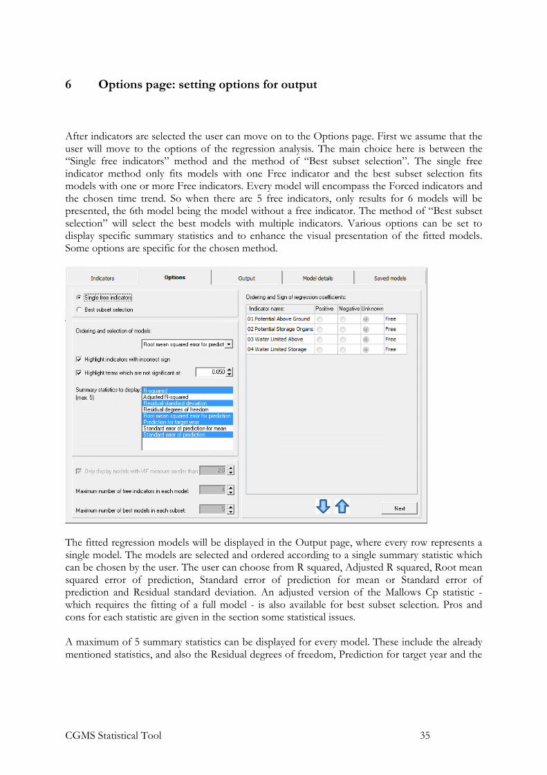
After indicators are selected the user can move on to the Options page. First we assume that the user will move to the options of the regression analysis. The main choice here is between the “Single free indicators” method and the method of “Best subset selection”. The single free indicator method only fits models with one Free indicator and the best subset selection fits models with one or more Free indicators. Every model will encompass the Forced indicators and the chosen time trend. So when there are 5 free indicators, only results for 6 models will be presented, the 6th model being the model without a free indicator. The method of “Best subset selection” will select the best models with multiple indicators. Various options can be set to display specific summary statistics and to enhance the visual presentation of the fitted models. Some options are specific for the chosen method.
The fitted regression models will be displayed in the Output page, where every row represents a single model. The models are selected and ordered according to a single summary statistic which can be chosen by the user. The user can choose from R squared, Adjusted R squared, Root mean squared error of prediction, Standard error of prediction for mean or Standard error of prediction and Residual standard deviation. An adjusted version of the Mallows Cp statistic - which requires the fitting of a full model - is also available for best subset selection. Pros and cons for each statistic are given in the section some statistical issues. A maximum of 5 summary statistics can be displayed for every model. These include the already mentioned statistics, and also the Residual degrees of freedom, Prediction for target year and the

CGMS Statistical Tool 36
Maximum of the Variance Inflation Factors (VIF) of the indicators. The use of the VIF is described in the some statistical issues section. In case of calibration mode some statistics, for which the predicted yield is required, are not available for selection, ordering and display. These are Standard error of prediction for mean and the Standard error of prediction and logically the Prediction for target year. The right part of the screen displays the list of indicators and whether they are chosen as Forced or Free. On the basis of experience, the user may expect a certain sign for the coefficients for at least some of the indicators – please read more on this in the section some statistical issues. In such cases the user can set the expected sign of a regression coefficient by means of the radio buttons. The sign can be positive, negative or unknown. The column headers can be clicked to set all signs simultaneously. When the option “Highlight indicators with incorrect sign” is checked, all regression coefficients with the incorrect sign will be highlighted in the Output page. When the sign is set to Unknown no highlighting will occur. It is also possible to highlight indicators for which the corresponding estimate is not significant at an adjustable level. These options can help to select an appropriate regression model. For the method of best subset selection, three extra options are available. The search for the best models can be subject to an optional constraint, set by the VIF option, on the degree of correlation permitted among the indicator variables. A higher value for the VIF measure allows models with a higher degree of correlation among the indicators; see some statistical issues. The maximum number of free indicators in every subset is limited by 4. This is to prevent the user to choose a model with too many indicators. Note however that - although not recommended - models with many indicators can be fitted by selecting a lot of indicators as Forced. Finally, the user can set the number of models to display for each subset. The branch and bound algorithm in the best subset algorithm (implemented to find the best model without fitting all models) requires that the full model, i.e. the model with time trend and all Forced and Free indicators, can be fitted. The full model cannot be fitted when the number of included years is less than the number of regression coefficients to be estimated for the full model, or when indicators themselves are linearly related. This is called aliasing of Indicators. In that case, after fitting the time trend, the selected Forced and Free indicators are added subsequently to the model. Indicators which cannot be fitted, either due to lack of sufficient years or due to linear relations among the indicators, are dropped from the list. The order in which indicators are added can be specified by the user by selecting an indicator and using the up and down arrows below the list of indicators. Indicators on top of the list are added first. In the case of scenario analysis, the Options page contains various options for making sure that the desired number of similar years is obtained, i.e. years which are similar to the selected target year.

CGMS Statistical Tool 37

CGMS Statistical Tool 38
7 Output page: viewing the results
Once all options are set in the Options page, the user can move on to the Output page. 7.1 Regression Models
In the case of Regression analysis, the requested method of single indicators or best subset selection is applied and results of the fitted regression models are displayed in the Output page. As a hypothetical example, consider a dataset for which a quadratic time trend was requested, indicator 01 was selected as Forced and indicators 02, 03 and 04 were selected as Free. Furthermore both types of highlighting were requested, with a significance level of 5% (default), and the models must be ordered according to root mean squared error of prediction. The sign of each regression coefficient was expected to be positive. The output for the method of single free indicators is given below. Every row represents a model and the second column lists which free indicator is included. The model indicated by “none” is without a free indicator. The header of the second column reminds the user of the chosen time trend and forced indicators. Next to the model are five summary statistics, indeed sorted according to the root mean squared error for prediction. The column denoted by “free indicator” contains the t value for the regression coefficient of the associated free indicator. The “linear term” column lists the t value for the linear and quadratic time trend, and the “01” column the t value for the forced indicator. The colouring of the t values either indicates a wrong sign of the coefficient (yellow) or a coefficient which is not significant (orange) or even both not good (red). Clearly, indicator 01 is never significant and the user might want to drop indicator 01 from the model. Although the R squared values of the 4 models are quite similar, the models give different predictions for the target year. The radio button in front of the first model and the green colour of the row indicates that this is the best model according to the chosen criterion. You can select a different model by clicking on the associated radio button.

CGMS Statistical Tool 39
The method of best subset selection presents the user with the following list of models.
The output is very similar to the output discussed before. The main difference is that more than one free indicator can enter a regression model. Every free indicator now has its own t value column with a value only when the associated free indicator is included in the model. The models are sorted according to the number of included free indicators, and within that by the requested summary statistic for ordering. The alternating colour of the rows, white or light grey, is used to distinguish models with 1, 2 3 or more free indicators. The model with 1 free indicator is better than the ones with only the forced indicator; and there is not much point in using a model with 2 or 3 free indicators. The best model is therefore the one with free indicator 02 with a significant t value; moreover the free regression coefficients have the correct sign. Note that for almost all models the linear and quadratic time trend are significant, but not the forced indicator 01. An analysis without indicator 01 might therefore be useful. In case the user wants to reproduce the results shown on the Output page elsewhere, he or she can copy the content of the window to the clipboard, by clicking first on the button “Copy to clipboard”, then paste into Excel or Word file. 7.2 Scenario models
The scenario analysis involves: first a Principal Component Analysis (PCA) on the indicator vectors, second a clustering of the years (for their classification based on distances in respect to the target year) and third, the yield prediction itself (based on the trend alone or on residuals of the similar years). In the PCA as many components are added as is it necessary to at least explain a given minimum level of variance. The components’ scores are then used to calculate a distance matrix. Such distances indicate how far in the Euclidian space a year is located away from other years. A set of years is then selected - on the basis of this matrix - which are closely located to the target year: the similar years.

CGMS Statistical Tool 40
Subsequently, for each year the residual with respect to the “none model” is calculated. The residual is defined as the difference between observed and estimated values. These residuals are summarized for the similar years and the non-similar years. On the right, the Output page shows first a table with the explained variance by each component. Next a table is presented containing the number of similar years and the number of non-similar years. In the same table, the minimum, average and maximum residuals are given for similar years and for the non-similar years respectively. Furthermore, the Output page shows results of three predictions, based on different methods. The first prediction is based on the time trend alone, without making use of residuals – therefore marked as “none”. The remaining two predictions are indeed made by means of the residuals. The forecast according to the time trend is taken into account, but it is corrected with a quantity:
• an average of the residuals of the similar years – marked as “Equally weighted residuals”
• a weighted average of the residuals of the similar years – marked as “Distance weighted residuals”.
The output of a typical scenario analysis is given in the figure below. The example pertains to barley in the Nord Ouest region of Morocco for the years 1999 to 2010 and with the year 2011 as the target year. Four CGMS indicators were included: Potential and Water Limited Above Ground Biomass and Potential and Water Limited Storage Organs. As can be seen, a linear time trend was selected. The top left section of the output page shows three statistics about principal components, explained variance and dissimilarity.

CGMS Statistical Tool 41
The mentioned weights are set to the inverse of the distances between each of the similar years and the target year. Weights are scaled by dividing each of them by their sum – i.e. they sum up to 1. In order to make sure that the residuals of years which are very similar to the target year would not exert a too great influence on the prediction, a maximum was introduced for the unscaled weights – default value for this is 50. From the three predictions, the one with the lowest residual standard deviation is selected. The residual standard deviation is the only criterion used for automatic selection from the three different models. The residual standard deviation is calculated by adding the sum of squares of the non-similar years to the sum of squares of the similar years. The latter is calculated by making predictions for each of the similar years in the same way as is done for the target year, i.e. a correction is calculated for each similar year on the basis of the other similar years. This is done for all the similar years, without calculating the distance matrix again. This means that the principal component analysis is done only once! The differences between the obtained predictions and the observed yields are then used to calculate the sum of squares of the similar years. 7.3 Saving model
The Save button at the bottom of the page can be used to save the settings and the results of the model indicated by the radio button. The results are in the first place saved to the database tables

CGMS Statistical Tool 42
RUN, FOREYIELD_HIS_REGION, MODEL_SETTINGS, MODEL_EXCL_YEARS, MODEL_INCL_INDICATORS, MODEL_REGR_INDICATIFS, MODEL_SCEN_ INDICATIFS and MODEL_SCEN_SIM_YEARS. More details on the structure and content of these tables can be obtained from the section 11.2 and from Annex 1. 7.4 Export settings
Finally, the user can export the settings to a setting file by using the export button at the bottom of the page. It should be noted that the analyst settings only store the choices made by the user at the time which formed the basis for the collection of models shown to him / her on the Output page. The analyst settings alone do not include any indication which model was selected and saved by the user at that time. When the option “Export” is chosen, first the user is prompted to enter a description for the selected model:
Next the user needs to indicate if the settings should be appended to the current selected file or to another file. In the latter case the user is prompted to choose a suitable location and filename. The save settings file, covering the settings for one combination of area, crop, dekad and analysis type can be shared with a colleague or analyst elsewhere, who is working on the same database. He or she can than reproduce the model (see section 11.4.2). It can also be used as a starting point to define multiple settings for running the CgmsStatTool in batch mode.

CGMS Statistical Tool 43
8 Model details page: viewing results of a selected model
8.1 Regression
Details of a model can be obtained by clicking on the blue link for that model in the Output page. The details are then displayed in the Model Details page which is opened automatically. One can copy the details, or parts of the details, and then paste them into Microsoft Word. The Model Details page for a regression model includes the following five sections:
• Description of model • Summary statistics • Regression coefficients • Confidence intervals for prediction • Case statistics • Plots
In the following, the above sections are dealt with in more details. For a higher level treatise of the statistical issues involved, see the next chapter entitled “Some Statistical Issues”. 8.1.1 Description of regression model
This section lists the area, crop, dekad, number of included years, start, end and target year. Also listed is whether the years have been transformed, the offset for the year effect and the time trend. For regression analysis an additional row is added which shows which indicators are included. 8.1.2 Summary Statistics
For regression analysis, the following summary statistics - with the page in MPV where they are defined - are listed:
• R squared: the percentage variance explained (MPV 39) • Adjusted R squared: the adjusted percentage variance explained (MPV 90) • Residual Standard deviation: the square root of the residual mean square (MPV 23) • Root mean squared error for prediction: define e(i) as the difference between the i th
response and the predicted value for the i th response based on a model fit to the remaining observations, i.e. without the i th observations. This is sometimes called the PRESS residual or the leave one out residual. The Root mean squared error of prediction is the root of the mean value of all the squared e(i). This is similar to the PRESS statistic (MPV 153).
• Maximum of VIF: the variance inflation factor of a regression coefficient is a measure of the degree of correlation between the associated indicator and the remaining indicators. Large correlations are equivalent to large variance inflation factor (MPV 337). This summary statistic is the maximum of the inflation factors for the indicators, i.e. the inflation factors for the constant and the time trend effects are not taken into account.

CGMS Statistical Tool 44
• Prediction for target year: the mean yield prediction for the target year according to the regression model (MPV 34).
• Standard error of prediction (Mean): the standard error of the mean yield prediction for the target year (MPV 34).
• Standard error of prediction (New): the standard error of the individual yield prediction for the target year (MPV 37). The following equality holds: SeNew2 = SeMean2 + ResidualStandardDeviation2.
• Residual degrees of freedom: the number of degrees of freedom for residual (MPV 23) In case of calibration mode some statistics, for which the predicted yield is required, are not available for selection, ordering and display. These are Standard error of prediction for mean and the Standard error of prediction and logically the Prediction for target year. 8.1.3 Regression coefficients
For regression analysis, this section lists the estimates of the regression coefficients, their estimated standard errors, the associated t values and two sided p values. To increase numerical precision, the regression coefficient for the linear time trend is for (year - offset) rather than year itself. The offset was fixed at 1965. Likewise, the regression coefficient for the quadratic time trend is for (year - offset)2. In case of a logarithmic transformation of the years, 1965 is also the default value for the offset, but in such cases the offset can be changed by the user to a certain extent. The p values are calculated by means of a Student distribution with degrees of freedom equal to the residual degrees of freedom. Finally the individual variance inflation factors (VIF) are listed. The VIF of an indicator is a measure of the degree of correlation between that indicator and the remaining indicators and time trend, if any, in the model. 8.1.4 Confidence intervals for prediction
Confidence intervals for the predicted value are given for confidence levels: 99%, 95%, 90%, 80% and 70% (band widths). Lower and upper bounds are calculated by firstly determining the t-value from Student's t distribution according the degrees of freedom and the one-sided cumulative probability and secondly multiplying the t-value with Standard Error of Prediction (New) and finally subtracting the value from (lower bound) and adding it to the forecasted yield. In case of calibration mode this table is empty. 8.1.5 Case statistics
For each included year the following case statistics are listed: • The yield • The fitted value according to the regression model. Note that the fitted value in the last
row equals the prediction for the target year • The ordinary residual which is the difference between the yield and the fitted value

CGMS Statistical Tool 45
• The leverage (MPV 209). Observations with large leverages are potentially influential because these observations have remote indicator values as compared to the rest of the observations. The mean of all leverages equals p/n in which p is the number of regression coefficients and n the number of observations. Leverages larger than 2p/n are traditionally considered as high leverage points. The leverage of the target year is of special interest because a target year with remote indicators will have a large standard error of prediction.
• The influence on the target year prediction. This is the difference between the predicted value for the target year based on the full dataset and the predicted value when the i-th observation is removed from the dataset. This is similar to the DFFITS statistics (MPV 214). In case of calibration mode this statistics is omitted.
8.1.6 Plots for diagnosing the model
The plots have a link to view the data in a separate window and through that window the user can copy the data for formatting graphs in an application like Excel. Two plots of case statistics can be used to check various aspects of the model:
• Observed (o) and fitted (x) values versus year. This plot is similar to the plot on the Time trend page, except that for excluded years no values are displayed at all. The plot can be used to check the observed and fitted yields. Note that for the target year only the predicted value is displayed; the prediction can thus be compared with the observed yields.
• Residuals versus fitted values, with an added horizontal line at y=0. The residuals should be evenly distributed for every fitted value. For example, when the residuals spread more for higher fitted values this indicates that the variance of the observations is not homogeneous (MPV 140).
Next, the following plots are shown:
• Normal probability plot of the studentized residuals (MPV 134) with a straight line to aid interpretation of the plot. The expected normal scores Φ-1 [(i 0.375) / (n+0.25)] are used, see McCullagh and Nelder (1989), and the points must roughly lie on a straight line. Although normality in itself is not an important assumption, a normal probability plot is still useful to identify outliers (MPV 138).
• Ordinary residuals versus year, with added horizontal lines at y=0 and at two sided cut off values with a p value of 0.95. The residuals should not have a relationship with year. A linear or quadratic plot might indicate that a time trend should be added to the model. The plot can also reveal that the variance is changing with time, or that residuals are correlated (MPV 146).
• Leverage versus year, with an added horizontal line at 2p/n. This plot can be used to identify observations that are potentially influential.
• Influence on the target prediction versus year, with horizontal lines at 2 x √ (p/n) x √ (LevN x RMS), where LevN is the leverage for the target year and RMS is the residual mean square. This plot shows the effect of deleting individual observations on the predicted value for the target year. A point can be influential on the regression model as a

CGMS Statistical Tool 46
whole, but have a small target prediction residual. See MPV 214 for the cut off value. In case of calibration mode this plot is omitted.
8.2 Scenario analysis
The Model Details page for scenario analysis, includes the following sections: • Description of model • Principal Component Analysis – parameters • Principal Component Analysis – loadings • Principal Component Analysis – statistics • Cluster Analysis • Analysis of residuals • Summary statistics • Prediction • Case statistics
8.2.1 Description of scenario model
This section lists the area, crop, dekad, number of included years, start, end and target year. Also listed is whether the years have been transformed, the offset for the year effect and the time trend. The last row indicates which of the models was selected: the one based on the time trend only (“none”), also on the “equally weighted residuals” or also on the “distance weighted residuals”. 8.2.2 Time trend coefficients
For scenario analysis, this section only lists the estimates of the time trend coefficients. 8.2.3 Principal Component Analysis - parameters
The following parameters are given: • Number of principal components • Percentage of explained variance • Number of observations used.
8.2.4 Explained variance
This table shows the explained variance by each component. 8.2.5 Principal Component Analysis - loadings
This table shows how the components are composed of the original indicators. The components are always linear combinations of those original indicators and the so-called loadings are therefore the relevant coefficients.

CGMS Statistical Tool 47
8.2.6 Clustering of years
To identify the cluster of similar years the following results are relevant: • the cutoff scores used • maximum Euclidian distance to the target year, among the similar years (thus the less
similar year in upper right cell) • the number of similar years found (lower right cell)
8.2.7 Overview of residuals relative to the trend
In this table similar years are placed versus the non-similar (other) years by showing some simple statistics of the residuals of the two sets of years. 8.2.8 Summary Statistics
For scenario analysis, only the following statistics are listed: • R squared: the percentage variance explained (MPV 39) • Residual standard deviation: the square root of the residual mean square • Prediction for target year: the yield prediction for the target year according to the time
trend and corrected with a linear combination of residuals pertaining to the similar years • Prediction for target year, minimum value: the yield prediction for the target year
according to the time trend corrected with the lowest residual available for the similar years
• Prediction for target year, maximum value: the yield prediction for the target year according to the time trend corrected with the highest residual available for the similar years
• Residual degrees of freedom: the number of degrees of freedom for residual (MPV 23) R-squared and residual standard deviation is calculated by adding the sum of squares of the non-similar years to the sum of squares of the similar years. The latter is calculated by making predictions for each of the similar years in the same way as is done for the target year, i.e. a correction is calculated for each similar year on the basis of the other similar years. This is done for all the similar years, without calculating the distance matrix again. This means that the principal component analysis is done only once! The differences between the obtained predictions and the observed yields are then used to calculate the sum of squares of the similar years. 8.2.9 Prediction
This section shows the following per similar year: • the Euclidian distance to the target year • the weight for the similar year • the residual for the similar year • the contribution of the similar year to the correction; i.e. the product of weight and
residual

CGMS Statistical Tool 48
8.2.10 Case statistics
This section shows the following for each year: • Euclidean distance • Observed yield • Fitted yield based on the selected model • Residual
This table can easily be copied and pasted in Excel to for instance sort on the Euclidean distance to analyze the distance in relation to the clustering of years. 8.2.11 Plots for diagnosing the model
The plots have a link to view the data in a separate window and through that window the user can copy the data for formatting graphs in an application like Excel. The plot of case statistics can be used to check various aspects of the model:
• Observed (o) and fitted (x) values versus year. This plot is similar to the plot on the Time trend page, except that for excluded years no values are displayed at all. The plot can be used to check the observed and fitted yields. Note that for the target year only the predicted value is displayed; the prediction can thus be compared with the observed yields. In case of no trend, all the non-similar years have the same fitted yield. In case there is a trend, the fitted yields for those years follow the trend.
• Dendrogram: a tree diagram used to illustrate the arrangement of clusters of years; to obtain the clusters, the clustering algorithm developed by Ward was used (Ward, 1963) with Euclidean distance as the type of distance measurement. The dendogram is based on a hierarchic cluster method and therefore leads to clusters of years that are not necessarily similar to the identified single group of similar years. The dendogram is an additional result to evaluate different groups of similar years.
• One or more plots of factor scores: in case of 2 principal components, only one plot is shown, in case of more components three plots are shown. Ovals are drawn in the plots, indicating the two cut-off distances used in the cluster analysis. Those ovals are really circles with radii equal to the respective cut-off values, i.e. the factors all have expectation 0 and variance 1.

CGMS Statistical Tool 49
9 Saved Models
The Saved Models page gives an overview of the different models and associated predictions saved for the selected area, crop and period (dekad). The Saved Model page mainly shows information of the saved model like the prediction, summary statistics and when and who saved the model. The page does show which models were selected by the user at various points in time. Over time, the user may have selected alternatives (e.g. different indicators, different trend models etc) for one and the same area, crop and period. The user may have even saved the same model and associated predictions for the same area, crop and period before and after an update was applied to the crop yield or indicator data. Only the results are used which were available at the moments the models were saved and stored. Please note that the models showed in the Saved Models page may pertain to different target years! The Saved Models page allows the analyst to compare the various models and associated predictions. Besides the predicted crop yields themselves, the following statistics pertaining to the model are shown: residual standard deviation, R squared and residual degrees of freedom. By means of these statistics the models can be compared – irrespective of whether they are regression models or scenario models.

CGMS Statistical Tool 50
Each of the displayed models can be selected by checking the radio button in the first column and then the model can be viewed, renamed or deleted. When the user indicates that he / she wants to view the selected model, the programme has to retrieve data about crop yields and indicators. A warning is then given: “Results may differ from those stored as a result of updates to the yield and indicator data”. No mechanism was built into the programme though to actually check whether there are any differences between the stored predictions and statistics and the results of the calculations based on the data from the database at the moment of retrieving the saved model. At that point, the programme has to also use the analyst settings to restore the model to its memory and to show the Model Details page for the selected model.

CGMS Statistical Tool 51
10 Some Statistical Issues
In this chapter, the statistical background is explained of the model selection as is facilitated by the CgmsStatTool. In section 10.1, various summary statistics for use in regression analysis are described, with their advantages and disadvantages for arriving at a stable prediction model. In section 10.2, it is described what the “best subset” algorithm involves and why it was chosen for the tool. Section 10.3, 10.4 and 10.5 describe some of the pitfalls related to model selection, particularly for regression analysis. Besides statistical principles, past experience is also relevant for model selection. Past experience has shown that, within the CGMS framework, time trend is generally the most important indicator. It is therefore that the user must specify a time trend (none, linear or quadratic) before any other element is added to the model. In case of regression analysis, the expected sign of the regression coefficients for some indicators may be known, also due to past experience. Estimated coefficients with a wrong sign can therefore be highlighted as an indication that the model might not be correct. In general, one should always try regression analysis first in order to arrive at a stable prediction model. Prediction models based on regression analysis are particularly useful for large areas, for years with more or less usual weather. Adverse weather conditions rarely occur over larger areas and do not usually also affect larger areas in the same unfavourable way. A dry period may e.g. cause yield reductions on certain types of soil, whereas it may be favourable on other soils which are generally subject to high groundwater tables. Therefore drastic yield reductions and even complete crop failures are often averaged out easily. For countries with a rather even climate, the time trend alone already gives a good fit and adding an extra indicator to the regression model often does not improve the model much. On the other hand, for countries with a rather whimsical climate adding an extra indicator may improve the model considerably. Scenario analysis is expected to be particularly useful for smaller areas, for years with exceptional weather. Section 10.6 contains more considerations on scenario analysis. 10.1 Selection of the Best Model
There are various methods for choosing a regression model when there are many indicators. Commonly used methods are forward selection, backward elimination and stepwise regression (MPV 310). However these methods result in only one model and alternative models, with an equivalent or even better fit, are easily overlooked. Moreover, the particular indicators that affect the response and the directions of their effects are of intrinsic interest and then selection of just one well-fitting model is unsatisfactory and possibly misleading. Therefore both the single indicators and the best subset selection methods present the user with several models. However, any selection method should be used with caution, especially when the number of indicators is

CGMS Statistical Tool 52
large in comparison with the number of observations. In this case uncritical model selection might lead to models which appear to have a lot of explanatory power, but contain noise variables only, see e.g. Flack and Chang (1987). Indicators should therefore not be selected on the basis of a statistical analysis alone. Experience with the intended use of the model, i.e. prediction for a target year, is therefore very important. As mentioned above, the sign of coefficients may be known from past experience. Wrong signs can be due to collinearity among the indicators, or because other important indicators have not been included in the model (MPV 120). Because the principal aim of the CGMS statistical system is to provide a reliable prediction for the target year, it should be noted that models with as few indicators as possible generally have better predictive power than models with many indicators. This can easily be understood when one realises that the more indicators are included in the model, the more coefficients will have to be estimated and therefore the more uncertainty is built into the model. The significance level of a regression coefficient indicates whether the corresponding indicator is necessary or not. Non-significant indicators can therefore be highlighted. So using highlighting both for sign and significance can be employed to select a model for which none of the regression coefficients is highlighted, although this might be too restrictive in practice. Several summary statistics can be used to initially select a best model (MPV 296). Any statistic will generally be overoptimistic because a lot of models are fitted in the process, especially for best subset selection, and the best model can be a stroke of luck. In any case, R squared is not a good criterion to select the best model because it will always select a model with the maximum allowed number of indicators. That is because R squared always improves by adding an indicator to a model. To put this another way, there is no penalty for adding an indicator. When Adjusted R squared or Mallows Cp is used there is a penalty for adding an indicator. Adjusted R squared improves when the absolute t value of the added indicator is larger than 1, while Cp improves when the absolute t value is larger than √2. Clearly Cp is the more conservative criterion and will tend to select models with fewer indicators as compared to R squared and R squared adjusted. The Cp statistic also has another rationale. Assume that the full model, i.e. the model with all indicators, provides a good estimate of the residual variance. Then the expected value of the Cp statistic for a smaller model with no bias equals the number of regression coefficients. So Cp can be compared to the number of coefficients (including the constant). However when the number of indicators is large as compared to the number of observations, the full model will often overestimate the residual variation and consequently the values of the Cp statistic will be small (MPV 300). The Root mean squared error of prediction has an intuitive appeal for the CGMS Statistical Tool because it specifically aims at small prediction errors. It is commonly used for model selection. The standard error of prediction for the target year is an unconventional summary statistic. It is not known whether this criterion provides stable and reliable predictions. The standard error of prediction for a new observation seems more appropriate than the standard error for the mean because the aim of CgmsStatTool is to predict a new observation. The above remarks can be summarized as follows. Incorporating knowledge and experience in the process of selecting a best regression model is extremely important. When the number of observations is small as compared to the number of indicators, careful model selection is crucial. In such a case, automatic methods with all indicators might well select a model which appears to be very good but will have low predictive power. For that reason, a careful pre selection of

CGMS Statistical Tool 53
indicators is necessary. The sign and significance of regression coefficients might provide clues as to which models are good. 10.2 The best subset model may not always be the best
The interface suggests that the method of best subset selection will always display the best models according to every summary statistic. However the algorithm used selects the best 40 models in every subset according to R squared. This is by definition equivalent to the best models according to R squared adjusted and Mallows Cp, but not always equivalent to the best models according to other summary statistics. For the 40 models thus selected, the other summary statistics are calculated and the models are sorted according to the requested statistic. Since a maximum of 10 models is displayed for every subset, it is likely, though not necessary, that these are the best models for every criterion. In theory however the best model according to one of the other statistics can be missed by the algorithm. So why not use another algorithm? One could of course fit every possible subset in turn to select the best model according to any criterion. However with 20 free indicators there are 4845 possible models with maximally 4 indicators; with 30 free indicators there are even 31930 possible models. Clearly the computational burden would then be enormous. The algorithm used in CgmsStatTool however does not explicitly fit all models, but uses a branch and bound algorithm to find the best models. This implies that it is very efficient even for large numbers of indicators. It was therefore decided to use this algorithm. The minor disadvantage of possibly not selecting the best model according to any criterion is taken for granted. The best subset algorithm used is the 1981 double precision version of a branch and bound algorithm for subset selection developed by Furnival and Wilson. This Fortran algorithm was obtained in 1982 by personal communication with Furnival and Wilson, see Ter Braak and Groeneveld (1982). It was claimed that the 1981 version is twice as fast as the 1974 version (Furnival and Wilson, 1974) and requires much less storage. From 1992 onwards, the best subset algorithm is also made available in Genstat by means of procedure RSELECT, see Goedhart (2005). Besides, the original Mallows is no more used in the CgmsStatTool for sorting and selecting the best model. Instead an adjusted or corrected Mallows Cp is used as introduced by Gilmour (1996). The best model is selected from the best models of the subsets: with each increase in the number of indicators it is checked whether the corrected Mallows Cp decreases at least 10%, otherwise the selection process stops and the model from the previous subset is selected. The criterion of at least 10% decrease in Corrected Mallows Cp was introduced on the basis of practical insights. 10.3 Multicollinearity and Variance Inflation Factors
Indicators are said to be multicollinear, or collinear, when there are near linear dependencies among the indicators (MPV 117 and 325). Near linear dependence can occur when there are many indicators as compared to the number of observations, or in case some indicators

CGMS Statistical Tool 54
essentially measure the same aspect as other indicators. An simple example is the mean temperature between 7 and 19 hours and the 24 hours daily temperature. Collinearity results in very large variances and covariances for the estimators of the regression coefficients. This implies that a small perturbation of the data might give very different estimated regression coefficients. Regression models with collinear indicators may therefore perform poorly when used for prediction purposes. One way to identify collinear indicators is that the sign of the estimated regression coefficients is wrong, or that the estimate is very large. This can simply be explained by the following example. Suppose that a response Y is, except for random error, linearly related to an indicator Z1 in the following way Y = 1 + 2xZ1. Suppose further that another indicator Z2 almost measures the same as indicator Z1, i.e. Z2 ≈ Z1. In that case Y = 1 + 2xZ2 is more or less equivalent to the model with Z1. But Y = 1 + 1xZ1 + 1xZ2 is also alike, and so is Y = 1 + 100xZ1 – 98xZ2. It turns out that all models for which the sum of the regression coefficients for Z1 and Z2 equals 2 are equivalent. As a result the estimated regression coefficients can be almost anything, depending on the specific observed values for Y, Z1 and Z2. Consequently, the variances of the estimates are generally large. A useful measure of collinearity is the variance inflation factor (VIF). Define Rj
2 as the R squared value of a regression model of indicator j on all the remaining indicators. The VIF of indicator j is then defined as 100 / (100 – Rj
2)-1. If indicator j is unrelated to the remaining indicators, Rj2 is
small and the corresponding VIF will be close to unity. However when indicator j is linearly related to some subset of the remaining indicators, Rj
2 will be close to 100 and the VIF will be very large. It can be shown that the estimated variance of the regression coefficient for indicator j scales with VIFj. Clearly one or more large VIF values is indicative for collinearity. MPV claim that “practical experience indicates that if any of the VIFs exceeds 10, it is an indication that the associated regression coefficients are poorly estimated because of multicollinearity”. The maximum VIF of all indicators is thus a good summary statistic for a regression model. Note that in calculating the individual VIFs the time trend model is also taken into account. However since year and year2 are themselves heavily correlated, even when an offset is first subtracted, the VIFs of the linear and quadratic time trend can be very large. This can be easily remedied by using orthogonal polynomials in which case the VIFs are equal to 1. This implies that VIFs for polynomial models are not very informative. Consequently, the maximum VIF of the regression model does not take the VIFs of the linear and quadratic time trend into account. The method of best subset selection has an option to only select models with a maximum VIF smaller than an adjustable value. This can be useful when all the best models have very large maximum VIFs. By specifying a smaller maximum VIF value a deeper search for the best model can be enforced. 10.4 Regression Diagnostics and Case Statistics
Something is “wrong” with most regression models: a high leverage point, a large residual, a VIF which is somewhat large, a normal probability plot which is not a straight line, residuals that tend to become larger when the fitted value increases, an observation that has a large effect on the predicted value for the target year. Automatic removal of observations to remedy the problem is

CGMS Statistical Tool 55
usually not a good idea. Deleting such points does improve the fit, but might result in a false sense of precision of the estimated regression model and thus of the prediction for the target year. Instead it is important to first find out why a certain problem occurs, and then take an appropriate action. It should be noted that the cut off values in the diagnostic graphs usually identify more observations than the data analyst is willing to verify. This is especially the case in small samples. Moreover, after removal of one point, sometimes another observation may suddenly stand out as problematic. In the discussion below a distinction is made between case statistics for outliers and for influential observations. Outliers are observations with a response which is not typical of the rest of the data. They can generally be identified by looking at residuals, although multiple outliers might mask each other. It is important to try to understand why an outlier has occurred. Perhaps the yield of a crop is incorrectly recorded in a certain year, or the yield is very low because of extreme weather conditions which are not representative for the year for which a prediction has to be made. In such cases there is evidence that something is wrong with the observation and it can be safely removed from the dataset. However when there is only statistical evidence that the observation is outlying, one should think twice before deleting the observation. MPV (154) note that “there should be strong non-statistical evidence that the outlier is a bad value before it is discarded”. Because the main aim of CgmsStatTool is to provide a prediction for the target year, the Influence on the target year prediction might be helpful in deciding whether to remove an observation or not. When there is only a small effect of removal of an outlier on the predicted value, one might want to keep the observation in the dataset. Influential observations have a more than average effect on summary statistics and /or on the estimates of the regression coefficients. One can distinguish between leverage points and influential points as shown in the Figure below.
A leverage points has remote values for the indicators, but the regression line does not change much by deletion of the leverage point. Such a point can be identified by a large leverage and a small residual, and also a small target prediction residual. An influential observation on the other hand also has a large leverage, but now both the residual and the target prediction residual is also large. Discarding of influential observations is therefore always worth considering, while leverage points can be possibly left alone. Whether an influential observation should be discarded is analogous to the treatment of outliers. MPV (218) note that “if analysis reveals that an influential point is a valid observation, then there is no justification for its removal”.
D A
Multiple casesLeverage point
C
A
Influential observation
B
A
Indicator Indicator Indicator
Yiel
d

CGMS Statistical Tool 56
All regression diagnostics implemented in CgmsStatTool are calculated for individual observations. However Cook and Weisberg (1982) note that “it can happen that a group of observations will be influential, but this influence can go undetected when cases are examined individually”. They illustrate this with the Figure on the right which is displayed above. If Point C or D is deleted, the fitted regression will change very little, while if both are deleted the estimates may be very different. Conversely, if A or B is deleted the fitted line will change, but if both are deleted the fitted line will stay about the same. This is simple to detect when there is only one indicator, but very hard when there are multiple indicators. Various suggestions have been made to identify groups of influential observations, among which certain forms of cluster analysis (MPV 217), but none of these have been implemented. 10.5 Perfect Fit and Aliasing of indicators
When a chosen time trend model whether constant, linear or quadratic provides a perfect fit to the yield data, the residual mean square of the regression model is zero. In this case a warning will be issued in the log window as soon as the data are processed for display on the Time trend page. Moreover the Time trend page will not display p values for the linear and quadratic time trend. Also on the Output page the p values for linear and quadratic effects will be denoted by “alias”. In that exceptional case no prediction for the target year is provided. This is also the case when a model with one or more forced indicators fits the data exactly. So only when a model with a time trend and forced predictors does not fit the data perfectly, a prediction for the target year is calculated. When indicators are perfectly linearly related, they cannot enter the same regression model. This can be either due to linear relations by definition or by chance, or by too few observations in combination with too many indicators. When the sample size is smaller than the number of indicators to be included in the regression model, the indicators are aliased by definition. Every effort has been made to ensure that the software handles aliasing in a correct and understandable way. The single free indicator method and the best subset selection method deal with aliased indicators in a different way. The single free indicator will display all indicators in the Output Tab, and aliased indicators can be identified by the word “alias” in the t value columns. A detailed analysis of such a model, by clicking on the blue link of the model, will have missing values for the corresponding regression coefficients. The best subset selection method on the other hand will first remove all aliased indicators from the indicator list, and proceed with the remaining indicators. This is because the algorithm requires that the full model, with all indicators, has a positive mean squared error. Removal of indicators is according to the order of the indicators in the Options Tab, but note that forced indicators are added before free indicators. Removal of indicators is reported in the log window. As an example suppose that there are 6 indicators with the following linear relations 05 = 01 + 02, and 06 = 03 + 04. The table below list which indicators are aliased in different situations. Order of indicators Free Forced Aliased 01 02 03 04 05 06 01 02 03 04 05 06 05 06 01 02 03 04 05 06 01 02 03 04 05 06 02 04 01 02 03 04 05 06 01 04 05 02 03 06 04 05

CGMS Statistical Tool 57
02 05 03 01 06 04 01 02 03 04 06 05 01 04 10.6 Comments on scenario analysis
Usually, crops have certain optimum conditions under which they thrive well. Too dry or too wet may cause similar yield reductions. The same is true for other variables such as temperature. Scenario analysis aims to identify historical years during which the agro-meteorological conditions were similar to the target year. The scenario approach is especially meant for predicting the yields during years with exceptional weather. The time trend is supposed to represent the general tendency for “normal” years. It should be realized that there are often certain growth stages during which crops are more sensitive to abnormal conditions than usual. The flowering stage is of course the most obvious example. At times, small changes in the sequence of meteorological events have major effects in crop response. It is recommended that the selection of indicators for Principal Component Analysis is done based on “non-statistical insights”. A nice set of similar years which seem similar may easily be obtained by clicking a few buttons. However, if those years are not really similar to the target year, one may end up predicting a higher yield than the time trend would suggest whereas the agro-meteorological conditions would rather suggest a lower yield than usual! After establishing a set of similar years, it is good to check why they are marked as similar. Are there years which are very similar to the target year and others less similar? The case statistics with the distances can answer this question. Which indicators contribute considerably to the selected factors? The table with the loadings can answer this question. And would there be a causal explanation as to how those indicators could affect crop yield in a favourable or unfavourable way? Maybe such explanations cannot be given for all indicators used in constructing the selected factors. A found similarity should be regarded as real when many of the included indicators have indeed got similar values for all the so-called similar years. When a causal explanation can be pointed out also as to how the crop yields could be affected, a similarity should be regarded as meaningful. In that case, the similar years are expected on one side of the trend line – i.e. in the plot of yields versus time. The current implementation of criteria R-squared and residual standard deviation - as used for automatically selecting the best model – will be evaluated at a later stage. Possibly a better criterion can be found for this, for instance by implementing a leave-one-out procedure including a re-calculation of the PCA and distance matrices.

CGMS Statistical Tool 58
11 Installation, databases and file menu
In the following the installation, the database and file menu will be described. 11.1 Installation
CgmsStatTool will be installed by default on the following directory: C:\Program Files (x86)\Alterra\CgmsStatTool (in the case of Windows 7). Under this directory you will find the following sub-directories:
• Doc: includes this user manual • Extra: software to create a Data Source Name entry for an MS Access database
(CreateDsnToMdb.exe) • Images: images supporting the user interface • Log: application error messages • Queries: queries used to retrieve data from the database • Resources: miscellaneous files e.g. statistics.txt which describes the codes for the
summary statistics to be displayed of a selected model On the main directory the following files are present:
• CgmsStatTool.exe: the CgmsStatTool • DFORRT.DLL: Visual Fortran Runtime library • StatLevel3.dll: the Fortran DLL responsible for determining the models • Files dbxadapter30.dll, dbxora30.dll and dbxoodbc.dll for connecting to database systems
MS Access and Oracle. The installation also copies the following files to the system folder: dbrtl100.bpl, DbxClientDriver100.bpl, DbxCommonDriver100.bpl, DbxDynalinkDriver100.bpl, DbxMetaData100.bpl, DbxReadOnlyMetaData100.bpl and rtl100.bpl. Besides, files are installed under the Public Documents Folder, also known as Shared Documents Folder or Common Documents Folder. It was decided to store the files and the data under the Public Documents Folder because it is the location that is most accessible for users than any other on the C-drive, i.e. less often restricted by permissions. The exact location of this folder varies from one Windows version to another: On Windows 7 this folder can be found here: C:\Users\Public\Documents\. The configuration options of CgmsStatTool (CgmsStatTool.ini; see Annex 4) are located below this Public Documents Folder, in the path Alterra\CgmsStatTool\. Finally, the CgmsStatTool is supplied with a sample Access database, CST_300.mdb, which can be found under the Public Documents in the path \Alterra\data\. The ODBC link called “CGMS local database” that is created during installation refers to this CST_300.mdb. See for

CGMS Statistical Tool 59
more information on changing database via ODBC Annex 2 and the wiki found here: https://sites.google.com/site/cropyieldforecasting/home. 11.2 Database structure
The CgmsStatTool interacts with other tools and programmes via the database. Below an overview of the tables and their relationships:
The tool retrieves data from a database and results can be written to that database too. The database containing the yield and indicator data is assumed to contain at least the following tables:
• STAT_REGION • REGION • STAT_CROP • INDICATORS • INDICATOR_DATA • CROP_ INDICATOR_DATA • RUN • STAT_REGION_EXCLUSIONS • AGRICULTURAL_YEAR • CROP_CALENDAR

CGMS Statistical Tool 60
• SEASON_INFO In addition a view is needed called DATA_FOR_YIELD_FORECAST. By means of this view all the indicator data become accessible for the important components of the application. Even the indicator data which are not crop-specific become available by means of this view, i.e. for all crops for which there are records in the table STAT_REGION. Another view is needed called DUPLICATE_INDICATOR_DATA to check whether an indicator is used in both tables: INDICATOR_DATA and CROP_INDICATOR_DATA. In that case the user will be warned that an indicator can only be used one of the two tables. The table SEASON_INFO is used by the CST to store temporary information on dekad definition and accumulation periods. The structure of these tables and views is described in further detail in Annex 1. Besides, the following tables are required, if the user wants to save results of his regression or scenario analyses to the database:
• FOREYIELD_HIS_REGION • MODEL_EXCL_YEARS • MODEL_INCL_INDICATORS • MODEL_REGR_INDICATIFS • MODEL_SCEN_INDICATIFS • MODEL_SCEN_SIM_YEARS • MODEL_SETTINGS
The structure of these tables is also described in further detail in Annex 1. The table FOREYIELD_HIS_REGION stored the final forecast. The table MODEL_REGR_INDICATIFS stores the selected model almost completely and includes items like:
1. The selected start year; 2. The selected end year; 3. The offset used for the years; 4. The selected transformation for the years; 5. The selected time trend; 6. Coefficient of selected time trend; 7. A number of summary statistics for the selected model.
In addition, the tables MODEL_EXCL_YEARS and MODEL_REGR_ INCL_INDICATORS store:
1. The years which were excluded; and 2. The indicators which were included in the model and their coefficients

CGMS Statistical Tool 61
The following tables enable the user to save results of scenario analyses to the database: • MODEL_SCEN_INDICATIFS • MODEL_SCEN_SIM_YEARS
CgmsStatTool is supplied with a sample Access database (CST_300.mdb), containing all the mentioned tables and an empty database (CST_300_empty.mdb). CgmsStatTool was created with the Microsoft Access database platform as first target in mind, to be accessed via ODBC. A facility has been included to enable the user to switch database e.g. another MS Access file or other ODBC connections (see section 11.4). CgmsStatTool can work with a database created in Microsoft Access but also with a database managed by an Oracle system or by SQLite. Extra drivers have to be installed before the tool can connect to these latter two databases. These other database management systems have however not been tested to work with the tool in recent years. Annex 2 describes how the tool can be made to work with other databases via ODBC. In Annex 6 it is explained how the input tables of an empty database can be filled with data for a different region of interest. 11.3 Filling the database
In order to use the CGMS Statistical Tool for a new area, it is advisable to start with an empty database (CST_300_empty.mdb). Such a database is provided with the installation. The following 7 tables will need to be filled in the given order:
• REGION • STAT_CROP • INDICATORS • STAT_REGION • AGRICULTURAL_YEAR • INDICATOR_DATA • CROP_ INDICATOR_DATA.
Why this order needs to be followed is explained in Annex 6. The tables REGION, STAT_CROP and INDICATORS have to be filled first with appropriate records, meaning in particular that unique keys (numerical identifiers) have to be given to each crop and each geographical unit respectively. Without those unique keys in place, the tables STAT_REGION, INDICATOR_DATA and CROP_INDICATOR_DATA cannot be filled. Each of the seven tables stores particular data: REGION Contains the codes, names and hierarchy of the administrative
geographical units STAT_CROP Contains the codes and names of the crops STAT_REGION
Contains officially approved historical yields and areas under cultivation – or in other words acreages – per crop, per year, for each geographical unit. Note that areas are not obligated

CGMS Statistical Tool 62
but can be of interest to search for the most dominant areas INDICATORS Contains the codes and names of indicators AGRICULTURAL_YEAR Contains 1 record that defines the start month of the
agricultural year CROP_ INDICATOR_DATA
Contains indicators per crop for each dekad within each year, for each geographical unit
INDICATOR_DATA Contains indicators for each dekad within each year, for each geographical unit
More explanation how a database should be filled to make it suitable for use with the CGMS Statistical Tool is given in Annex 6. 11.4 File menu
In most cases the tool can be driven by selecting options offered in the left menu and options offered on one of the five tab pages on the right panel. However, the tool is equipped with a file menu for special actions. The menu has the following structure:
• File Change database; New settings file; Open settings file; Save settings as; Save model results; Export current settings; Print report; Exit;
• View Log Window; • Tools Data import and management; Test model for other dekads / regions;
Run; Save report to file; • Help User manual; About
11.4.1 File – change database
The file menu has the option “Change database”. When this option is chosen, a popup form appears – the “database switch form”. By default the CgmsStatTool connects to the so-called pre-configured sample database. That is the database that is indicated by means of an ODBC Data Source Name in the INI file – see also Annex 4. The tool has the possibility to connect to other databases, i.e. those that have their data in one file. Such databases are indicated as file-based databases. In the first place this possibility exists for databases managed by the MS Access database management system, which can handle files with the extensions “mdb” and “accdb”. When the user wants to connect to another, file-based database that is different from the pre-configured database, the user needs to click a number of controls on the “database switch form”:
1. Select the radio button “File-based database” 2. Navigate to the relevant folder using the drive selector and the directory list box located
on the left of the form 3. Click on the relevant database file in the grid located on the right 4. Press the “Switch” button at the button of the form and wait until the application reports
that the selected database is suitable 5. Press the “Close” button

CGMS Statistical Tool 63
It is advisable to only select database files with all the necessary tables inside. If a non-compatible database is selected, the application has to restart. By checking the box “Save database change to inifile”, the database change becomes semi-permanent. The next time the tool starts, it will no more open the pre-configured database but the newly selected one. 11.4.2 File – managing settings
At start up, the programme by default is linked to the file “CgmsStatTool.csv”. At the start this is an empty analyst settings file under the Public Documents Folder, in the path Alterra\CgmsStatTool. The user may want to load a different file with analyst settings. The file menu therefore has the options “New settings file” and “Open settings file”. When “New settings file” is selected, an empty CSV file is created. When the option “Open settings file” is selected, the user can select another file to work with. The “Open settings file” dialog always suggests the name of the currently loaded file. After selecting another file, the programme checks how many sets of analyst settings the file contains:
• If the file contains only one set of analyst settings (thus one set for one combination of an area, crop, period and analysis type), then the user is prompted with a question whether the settings should be loaded into the programme’s interface. In this case interface is completely reset according these settings.

CGMS Statistical Tool 64
• If the file contains more than one complete set of analyst settings, a message appears in the log window. Subsequently, the programme continues to work with the indicated file from then on, until it is terminated. To make use of these settings the user must first select the correct area and crop for which settings are available in the newly opened file. This is something the user needs to know in advance. Then the interface can be changed to these settings via the “retrieve settings” function (see section 3.4).
When a user does not open another settings file, exported settings (see section 7.4 for export) are written to CgmsStatTool.csv under My Documents. Each time the CgmsStatTool is start this default is replaced by an empty file. To save the settings that were exported during a session the user can save the CgmsStatTool.csv (via “Save settings as”) under a different name on a user defined folder. 11.4.3 File – miscellaneous
The “Save model results” and “Export settings” are similar to the functions described in section 7.3 and 7.4. These are only enabled when a regression or scenario has been carried out and the relevant output frame still has the results loaded. Any time the Output or the Model Details page is open, it is possible also to print whatever is shown there. The user can start printing to the default printer by choosing “Print report” from the File menu. In the case of the Model Details page, a print dialog appears first, in the case of the Output page it does not. In case the user wants to represent the information from the Output page in a way different from the way it comes out from the default printer, the button “Copy to clipboard” at the bottom of the Output page can be of help. When the option “Exit” is chosen, a dialog pops up asking for a confirmation that you really want to exit CgmsStatTool:
11.4.4 View
The only option under the “View menu” i.e. “Log Window” – can be used to show or hide the fourth optional panel with a log window which can contain informational messages, warnings and error messages. The log window always appears below the left and right panels. It can be right clicked after which a popup menu appears with the options Hide, Clear and Copy. If the latter option is chosen, always all the messages in the log window are copied to the clipboard. If only a few lines from the log window need to be copied to the clipboard, this can be done by selecting those lines followed by key combination Control C.

CGMS Statistical Tool 65
11.4.5 Tools
When the option “Data import and management” is chosen, a popup form appears with a few tab sheets. More explanation about the possibilities offered by means of this form is given in Chapter 13. The option “Test model for other dekads / regions” is offered to determine the best regression models for a number of dekads for a specific region in a batch processing. More details are given in section 12.2.3. The option “Run” can be chosen when a combination of area, crop and period is selected for which yield and indicator data are available. This option is only activated when at least one indicator is selected on the Indicators page. In principle it is always possible though to build a regression model based on the time trend alone. A report about the model can be saved in addition. The Model Details page needs to be opened. From the file menu the option “Save report to file” can be chosen or the last but one button on the toolbar can be pressed. Then the user is prompted to enter the name of the web archive in MHT format:
Such web archives can be opened in Internet Explorer and in Firefox and SeaMonkey browsers equipped with the UnMHT Add-On. When opened, they are supposed to show both text, tables and graphs as normally can be viewed in the Model Details page. 11.4.6 Help
This file menu gives access to the about window and the user manual.

CGMS Statistical Tool 66
12 Analyst settings and batch mode
12.1 Analyst settings
12.1.1 Format
A complete set of analyst settings, spanning in principle either 20 or 29 lines (for scenario and regression analysis respectively), is specific for a specific area, crop, dekad and analysis type. The model that has led to the prediction is not stored as such, but what is stored are the options selected by the analyst which led to that model, e.g. for regression analysis which indicators are included as free and which ones are included as forced indicators. Hence the analysis can be reviewed at any later time and if necessary it can be repeated with updated indicator data or even for the year following the one for which the analysis was carried out originally (if one changes the target year). All analyst settings are stored together with the area code, crop number, dekad and analysis type to which they apply. This can be either in the database or in a file. One single setting is: 1. a record in the table MODEL_SETTINGS is linked to a record in the table RUN with four
fields indicating area code, crop number, dekad and analysis 2. a line in the external settings file (comma separated values file) always starts with four fields
separated by a comma, indicating area code, crop number, dekad (currently still called decade) and analysis type respectively.
Annex 3 describes the analyst settings in further detail. It also gives more information on settings files can be managed and changed. It should be noted that the CSV format for storing these settings was chosen because it can be accessed by many programs in different ways, thus giving the user ample freedom to edit, copy, modify or share settings. When editing the file, the user however needs to make sure that the first five fields of every line are unique – i.e. area code, crop number, dekad number, analysis type and setting name. Otherwise, an error message “Duplicate index value. Operation aborted” will appear, when the user attempts to open the CSV file in CgmsStatTool. 12.1.2 Where do settings come from?
The user can export the settings to a settings file by using the export button at the bottom of the Output page (see section 7.4) or save settings to the database together with a specific model using the save button at the bottom of the Output page (see section 7.3).

CGMS Statistical Tool 67
12.1.3 How to retrieve settings?
At start up, the programme by default is linked to the file “CgmsStatTool.csv”. At the start this is an empty analyst settings file under the Public Documents Folder, in the path Alterra\CgmsStatTool (see section 11.1). This file is temporary and can be used to save one or more set of analyst settings during a session. It can also be save under a different name. To re-set the user interface to the previously saved settings the user either gets those settings from a file or from the database. In case the settings come from the file, the user selects a different file with one or more sets of analyst settings e.g. from a colleague or saved from a previous session. The file menu therefore has the option “Open settings file” (see section 11.4.2). There are two main strategies/effects:
1. If the file contains only one set of analyst settings (thus one set for one combination of an area, crop, period and analysis type), then the user is prompted with a question whether the settings should be loaded into the programme’s interface. In this case interface is completely reset according these settings
2. If the file contains more than one complete set of analyst settings, a message appears in
the log window. Subsequently, the programme continues to work with the indicated file from then on, until it is terminated. To make use of these settings the user must first select the correct area and crop for which settings are available in the newly opened file. This is something the user needs to know in advance. Then the interface can be changed to these settings via the “retrieve settings” function (see section 3.4). This function is also the way to re-set the interface based on settings that are stored in the database.
Below an example is shown of what happens when a user opens an exported file that has only one complete set of analyst settings.

CGMS Statistical Tool 68
12.2 Batch mode
The CgmsStatTool can also be used to construct regression models2 for one or more combinations of region, crop and dekad in a batch processing. This is useful to explore how certain models work for other dekads and/or regions or to find quickly the best models for each dekad and/or region. It can be done within an interactive session of the CgmsStatTool (see section 12.2.3) or separately via a command line operation (see section 12.2.4). Starting point is set of (interface) settings (see section 12.1 for more information). 12.2.1 Best model selected
In batch mode only the best model will be selected and returned. The criteria that determines the best model, is defined by the setting variable called “BestModelSelection”. The following models are excluded in advance:
- for which the variance inflation factor exceeds the setting variable “MaxVifMeasure” - that are wrongly correlated in case the setting variable “HighlightWrongSign” is activated
(= -1)
2 Currently the batch mode is not implemented for scenario analysis

CGMS Statistical Tool 69
- that are not significant in case the setting variable “HighlightIfNotSignificant” is activated (= -1)
12.2.2 Minimum number of years
The minimum number of complete years (all selected indicators have a value and yields are available as well) allowing the calculation of a regression model is given in the file CgmsStatTool.ini: [batch settings] MinNumAvailYears =6 12.2.3 Batch processing via interactive mode
Once a user defined all settings in the user interface and the CgmsStatTool returned possible models, the user can inspect the regression models in the Output page. Starting point of the batch processing now is to select the preferred model that the user would like to apply to other dekads and/or regions. In fact the settings that led to this list of models, will be copied to:
- a range of dekads for the same combination of region and crop - and/or another region for the same crop and a range of dekads
The option ‘Test model for other dekads / regions’ under the file menu ‘Tools’ supports the user in:
- copying and adjusting the settings - run the CgmsStatTool in batch mode - save results.
After activating this option the following settings view window appears (tab ‘duplicate settings’).

CGMS Statistical Tool 70
The window shows the current settings that led to the list of regression models in the Output page. The user can define a dekad range (start and end via the dekad selector on the right) to copy settings to each individual dekad in the range. Moreover, the user can copy the settings to another region but only those regions that belong to the same parent region as the one currently selected. Leaving the last two options, ‘Fix trend type’ and ‘Force indicators’, default (not selected) means that settings are copied without any change. In the current example (see above picture), with only free indicators and no forced indicators and a trend model being automatically defined, the selected model that will emerge for another dekad and/or region can have a different indicator and / or a different trend model. This option is useful to explore the best model given the selected options e.g. a list of free indicators, single/best subset, automating testing of trend type models etc. To apply exactly the same model to other dekads and/or regions the user can fix the indicator of the selected model (‘force indicators’) and the trend type (‘fix trend type’)3. These options are useful to test a certain model for other dekads and/or other regions. Note that if the user forces the indicator(s) in the model the CgmsStatTool will return these models even if they do not comply with the criteria listed in section 12.2.1. After confirming the choices (OK button), the user has to define a file to which the settings will be written. Afterwards a new window is presented to the user:
The user is asked whether he/she would like to run CgmsStatTool in batch mode using the settings file just saved (‘Apply and have the results saved to the database’). In addition the user can have the results exported to a CSV file for further analysis in for instance Excel (‘Export results to CSV so that they can be plotted in Excel’). After confirming the choices (OK button), CgmsStatTool executes all runs defined in the settings file and writes them to the CSV file. All the results that are written are independent of possible indicator data observed in the target year, meaning that the batch processing can be done interactively even in calibration mode. 3 Alternatively the user can change the settings in the user interface in such way that the CgmsStatTool always test the same model e.g. by defining only forced indicator(s) and/or force a time trend type

CGMS Statistical Tool 71
Once ready the user has to define a file to which the results will be written. The duplicate settings function can also be activated via ‘Retrieve Analyst Settings’ (see section 3.4 and section 12.1.3) but this only works if the user has loaded a settings file for one particular region, crop and dekad combination. 12.2.4 Command line
In this mode the CgmsStatTool constructs regression models for one or more combinations of area, crop and dekad using file-based settings for these combinations in an automated manner. Start in batch mode with: CgmsStatTool /batch <filename> This filename should have the same structure of a setting file (see section 12.1). The program searches for this settings file at the following locations in this order:
• directory where CgmsStatTool.exe is located • using the path that can be given in <filename> • using the PATH defined by Windows environment variable • AppDataFolder, e.g.: C:\Users\Public\Documents\Alterra\CgmsStatTool
A (batch) window is started. Behind the scenes, a regression analysis is done for each combination of area, crop and dekad included in the batch file. The settings file contains other choices as well, e.g. the intended target year4. 4 As yet, it is necessary that there are indicator data in the database for each given dekad of all relevant years – also for the indicated target year. It means that when the batch mode is run from the command line, it cannot run in calibration mode yet. In case batch processing is started from an inter-active session (option ‘Test model for other dekads / regions’ under the file menu ‘Tools’ ) the calibration mode does work and models can be derived without have indicator values for the target year.

CGMS Statistical Tool 72
In the window, the progress of the batch job is shown: Example: Started at: 31/05/2013 16:13:13 Run batchmode from: C:\Users\Public\Documents\Alterra\CgmsStatTool\CgmsStatTool.csv Number of settings read: 7 - [14.29%] ForecastRun( FRegMapId=10490, FStatCropNo=1, FTargetYear=2012, FDecade=14, FRunId=25 ) - [28.57%] ForecastRun( FRegMapId=10519, FStatCropNo=1, FTargetYear=2012, FDecade=14, FRunId=26 ) - [42.86%] ForecastRun( FRegMapId=10498, FStatCropNo=1, FTargetYear=2012, FDecade=14, FRunId=27 ) - [57.14%] ForecastRun( FRegMapId=10510, FStatCropNo=1, FTargetYear=2012, FDecade=14, FRunId=28 ) - [71.43%] ForecastRun( FRegMapId=10491, FStatCropNo=1, FTargetYear=2012, FDecade=14, FRunId=29 ) - [85.71%] ForecastRun( FRegMapId=10532, FStatCropNo=1, FTargetYear=2012, FDecade=14, FRunId=30 ) - [100.00%] ForecastRun( FRegMapId=10511, FStatCropNo=1, FTargetYear=2012, FDecade=14, FRunId=31 ) Finished at: 31/05/2013 16:13:21 Duration : 00:00:07 This info is also stored in the file CgmsStatTool_batch.log. Results of best forecasts are stored in the database. The final results are stored in the selected database. The user can retrieve results by applying specific queries. See an example query from a MS Access CgmsStatTool database below:
SELECT RUN.RUN_ID, STAT_CROP.STAT_CROP_NAME, REGION.REG_NAME, RUN.DECADE, MODEL_INCL_INDICATORS.INDICATOR_NAME, MODEL_REGR_INDICATIFS.RMSQ_ERR_PRED, MODEL_INCL_INDICATORS.COEF_TVALUE FROM STAT_CROP INNER JOIN (((REGION INNER JOIN RUN ON REGION.REG_MAP_ID = RUN.REG_MAP_ID) LEFT JOIN MODEL_INCL_INDICATORS ON RUN.RUN_ID = MODEL_INCL_INDICATORS.RUN_ID) INNER JOIN MODEL_REGR_INDICATIFS ON RUN.RUN_ID = MODEL_REGR_INDICATIFS.RUN_ID) ON STAT_CROP.STAT_CROP_NO = RUN.STAT_CROP_NO ORDER BY RUN.RUN_ID;
12.2.5 Process all best subset models
In the stand alone, inter-active, mode, for the best subset algorithm, the branch and bound algorithm is implemented to find the best model without fitting all models. This requires that the full model, i.e. the model with time trend and all Forced and Free indicators, can be fitted. The full model cannot be fitted when the number of included years is less than the number of regression coefficients to be estimated for the full model. In that case, after fitting the time trend, the selected Forced and Free indicators are added subsequently to the model. Indicators which cannot be fitted, either due to lack of sufficient years or due to linear relations among the indicators, are dropped from the list.

CGMS Statistical Tool 73
In situations where the user would like to test all indicators for instance in a batch processing, the CST does not apply the branch and bound algorithm but applies the so-called brute force approach: testing all models. Disadvantage of the brute force approach is the loss of performance because all models need to be evaluated. This becomes important when allowing more than 3 indicators in one model and using a relatively high number of indicators (>20).

CGMS Statistical Tool 74
13 Data import and management
When this option is chosen from the file menu “Tools”, a separate popup form opens. This form gives access to a toolbox that was integrated into the CgmsStatTool to facilitate data import and data management, esp. of the indicator data in the tables INDICATOR_DATA and CROP_INDICATOR_DATA. These two tables store data which are specific for area / region, year and dekad. One of the components in the toolbox is called Import RUM. It is particularly suitable for importing so-called RUM data as produced by the software tool SPIRITS developed by VITO in Mol, Belgium – see:
• https://rs.vito.be/africa/en/software/Pages/software.aspx • http://spirits.jrc.ec.europa.eu/
More information about the RUM format can be found here: http://marswiki.jrc.ec.europa.eu/agri4castwiki/index.php/Formats#Databases_of_regional_unmixed_means A second component is called Accumulate Data which can be used to calculate cumulative values of indicator data already available in the tables INDICATOR_DATA and CROP_INDICATOR_DATA. These cumulative values refer to a fixed start dekad and a moving end dekad. For instance: cumulating from dekad 1 to 3 means that sums are calculated for the period dekad 1 to 2 and period dekad 1 to 3. A third component is called Copy Data which can be used to make data which are available for a particular dekad also available for another dekad that occurs later in the same campaign /agricultural year. A fourth component is called Moving Sums which can be used to calculate cumulative values of indicator data already available in the tables INDICATOR_DATA and CROP_INDICATOR_DATA. These cumulative values refer to a fixed period and a moving start and end dekad. For instance: cumulating for a fixed period of 2 dekads means that sums are calculated for the period dekad 1 to 2, period dekad 2 to 3, period dekad 3 to 4 etc. A few important notes:
- In principle, these tools can help to fill both table INDICATOR_DATA and table CROP_INDICATOR_DATA. Once however the data of a particular indicator is inserted into any of these two tables, it is not possible to insert them again into the other table. This is particularly reflected in the values offered in the drop-down list showing the crops. If for the first time the option “All” is chosen in that list, the indicated data will be inserted into table INDICATOR_DATA. When the user tries to insert data for that same indicator again, only the option “All” will be offered. If however a specific crop is chosen for the first time, the indicated data will be inserted into table CROP_ INDICATOR_DATA – i.e. only for the indicated crop. When the user tries to insert data

CGMS Statistical Tool 75
for that same indicator again, only the names of separate crops will be offered for which there are already historical yields in the database, the option “All” is not offered.
- Furthermore in case the user would like to accumulate or copy data from a crop specific indicator (stored in table CROP_INDICATOR_DATA), the user can only select indicators that occur in table CROP_ INDICATOR_DATA or indicators that were not yet used in one of the two tables.
13.1 Import RUM
A relevant example screen is presented below. With this tool, the user can import a set of RUM files (field MEAN). One important assumption is that all RUM files describing one indicator (e.g. NDVI) are stored in one folder. That folder must not contain RUM files with data for other indicators. The following mappings, conversions and checks are done during the import:
• The set of RUM files of a selected folder are mapped to the indicator selected in the interface
• Each imported value is attributed to the dekad calculated from the date found on the relevant line of the RUM file.
• Only RUM data of the indicated land cover are imported; it means that the Import RUM tool reads all lines it encounters but only those lines are processed which pertain to the indicated land cover class.
• Lines with region identifiers which are not registered in the table REGION of the database are discarded.
• Missing values, indicated with -999.999, are discarded. The missing value can be changed in the CgmsStatTool.ini, section Miscellaneous settings

CGMS Statistical Tool 76
The following table explains in more detail how to use this interface:
Target database / DSN This is a read-only field that is meant to make the user aware of the database into which he / she is inserting data
Folder with input files In this box a valid path to the folder with the RUM files needs to be filled out. In principle the form opens with as default folder the parent of the folder from which RUM files were imported the last time. When the “Browse” button is pressed, a dialog appears that allows you to select a directory. Unfortunately, the dialog does not show any RUM files that may be present in the shown folders. However, the tool reports afterwards how many RUM files it has found in the selected folder with the indicated extension (usu. *.rum).
File extension This list is populated with the extensions of the various files the tool has found in the selected folder. When a different extension is selected, the tool reports how many files it has found in the selected folder with that extension. Usually the RUM extension is selected.
Land cover selection After selecting the right folder, this box can be filled by pressing the button “Scan input files for codes”. It is assumed that the input files contain data obtained by means of remote sensing. The aggregation of these data to a lower resolution (e.g. to region) is done in a land cover specific manner. When calculating the regional means only values of remote sensing pixels are selected that are covered by the selected land cover map. By selecting the right land cover here, the user can make sure he / she retrieves the mean values from the RUM files which are most relevant for the desired target crop.
Indicator code The drop-down list shows all the codes it can find in the database which are not write-protected. If the user wants to introduce a new indicator code, he/she can do so by pressing the button “New code”. There’s no need to restart the tool afterwards. The user is expected to select the code that he /she wants the tool to use for insertion of the indicator values.
Crop
Here the user can select the crop to which he / she wants to link the data of the selected land cover. This can also be the general type “All” (associated with table INDICATOR_DATA). In the latter case the imported indicator data can be used in regression and scenario models for all crops.
Overwrite existing records
The table INDICATOR_DATA or the table CROP_INDICATOR_DATA may already contain data for the same region, year, dekad, indicator and even crop. When this box is ticked, the tool will detect such data first, and delete them before trying to insert the new data. It is however not possible to have the data deleted from table INDICATOR_DATA and to then have the new data inserted into table CROP_INDICATOR_DATA or vice versa.
Memo In this field, messages are shown to inform the user about the success or failure of the requested operation. These messages appear in real time.
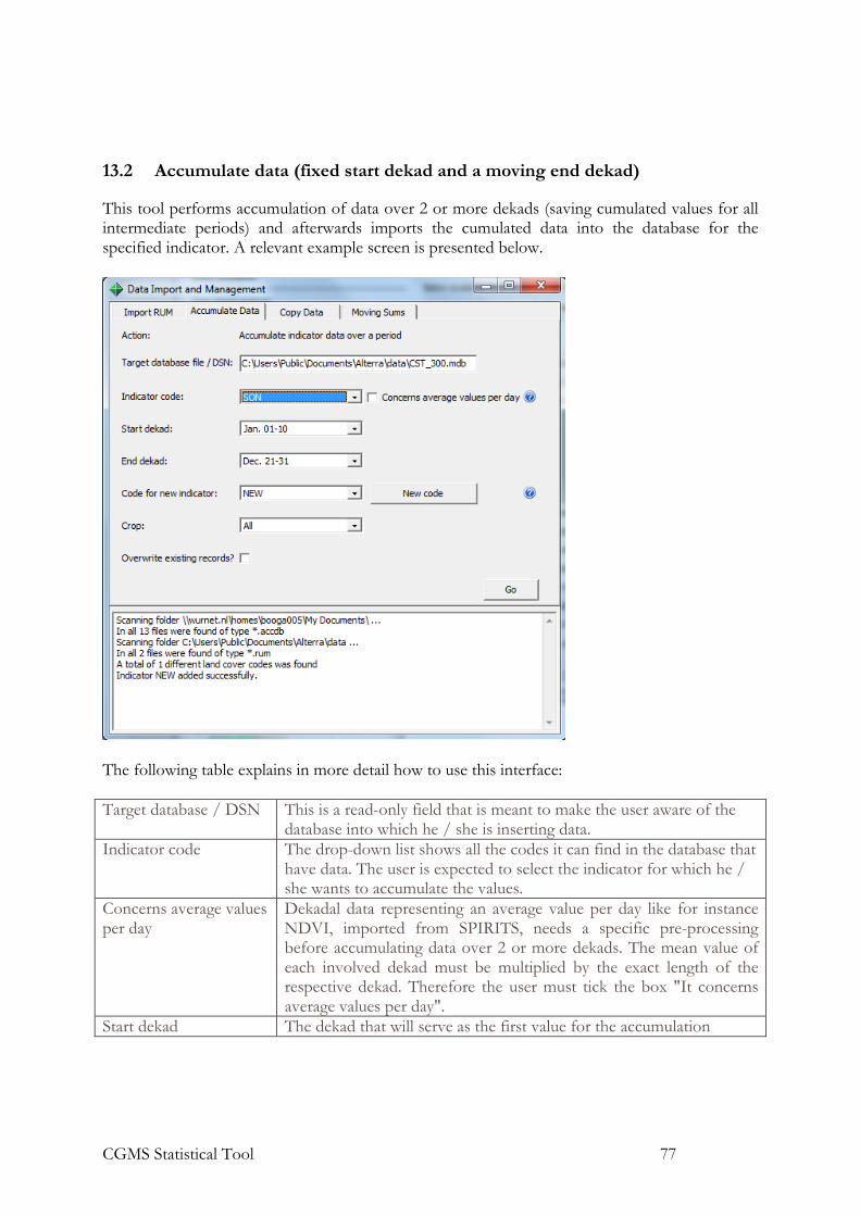
CGMS Statistical Tool 77
13.2 Accumulate data (fixed start dekad and a moving end dekad)
This tool performs accumulation of data over 2 or more dekads (saving cumulated values for all intermediate periods) and afterwards imports the cumulated data into the database for the specified indicator. A relevant example screen is presented below.
The following table explains in more detail how to use this interface: Target database / DSN This is a read-only field that is meant to make the user aware of the
database into which he / she is inserting data. Indicator code The drop-down list shows all the codes it can find in the database that
have data. The user is expected to select the indicator for which he / she wants to accumulate the values.
Concerns average values per day
Dekadal data representing an average value per day like for instance NDVI, imported from SPIRITS, needs a specific pre-processing before accumulating data over 2 or more dekads. The mean value of each involved dekad must be multiplied by the exact length of the respective dekad. Therefore the user must tick the box "It concerns average values per day".
Start dekad The dekad that will serve as the first value for the accumulation

CGMS Statistical Tool 78
process. End dekad The dekad that will serve as the last value for the accumulation
process. Code for new indicator The drop-down list shows all the codes it can find in the database
which are not write protected. If he / she wants to introduce a new indicator code, the user can do so by pressing the button “New code”. There’s no need to restart the tool afterwards. The user is expected to select the code that he / she wants the tool to use for insertion of the indicator values. The code selected here should preferably be different from the indicator code selected above.
Crop number Here the user can select the crop to which he / she wants to link the accumulated values. Which one is offered depends on the source indicator that was selected. See initial remark of this chapter.
Overwrite existing records
The table INDICATOR_DATA or the table CROP_INDICATOR_DATA may already contain data for the same region, year, dekad, indicator and even crop. When this box is ticked, the tool will detect such data first, and delete them before trying to insert the new data. It is however not possible to have the data deleted from table INDICATOR_DATA and to then have the new data inserted into table CROP_INDICATOR_DATA or vice versa.
Memo In this field, messages are shown to inform the user about the success or failure of the requested operation. These messages appear in real time.
13.3 Copy data
This tool retrieves data which are available for a reference dekad and inserts them into the database for a specified period and indicator. A relevant example screen is presented below.

CGMS Statistical Tool 79
The following table explains in more detail how to use this interface: Target database / DSN This is a read-only field that is meant to make the user aware of the
database into which he / she is inserting data Indicator code The drop-down list shows all the codes it can find in the database
which have data. The user is expected to select the indicator for which he / she wants to copy the values.
Reference dekad The dekad for which the indicator values are of particular interest. In the example, April 21-30 is selected during which low temperatures could affect the emergence of the crop and therefore the eventual yield. By copying these values to later dekads in the season, the user makes it possible to include this indicator into regression analyses for dekads later in the season.
Start dekad The dekad that marks the beginning of the period for which the indicator values are copied.
End dekad The dekad that marks the end of the period for which the indicator values are copied.
Code for new indicator The drop-down list shows all the codes it can find in the database which are not write protected. If he / she wants to introduce a new indicator code, the user can do so by pressing the button “New code”. There’s no need to restart the tool afterwards. The user is expected to select the code that he / she wants the tool to use for insertion of the indicator values. The code selected here should preferably be different from the indicator code selected above. For instance it would be

CGMS Statistical Tool 80
logical to have a new code that refers to the TMIN of April 21-30 Crop number Here the user can select the crop to which he / she wants to link the
copied values. It can be a specific crop or the generic term “All”. Which one is offered depends on the source indicator that was selected. See initial remark of this chapter.
Overwrite existing records
The table INDICATOR_DATA or the table CROP_INDICATOR_DATA may already contain data for the same region, year, dekad, indicator and even crop. When this box is ticked, the tool will detect such data first, and delete them before trying to insert the new data. It is however not possible to have the data deleted from table INDICATOR_DATA and to then have the new data inserted into table CROP_INDICATOR_DATA or vice versa.
Memo In this field, messages are shown to inform the user about the success or failure of the requested operation. These messages appear in real time.
13.4 Accumulate data (fixed period, moving start and end dekad)
This tool performs accumulation of data over a fixed period of 2 or more dekads and afterwards imports the cumulated data into the database for the specified indicator. A relevant example screen is presented below.

CGMS Statistical Tool 81
The following table explains in more detail how to use this interface: Target database / DSN This is a read-only field that is meant to make the user aware of the
database into which he / she is inserting data. Indicator code The drop-down list shows all the codes it can find in the database that
have data. The user is expected to select the indicator for which he / she wants to accumulate the values.
Concerns average values per day
Dekadal data representing an average value per day like for instance NDVI, imported from SPIRITS, needs a specific pre-processing before accumulating data over 2 or more dekads. The mean value of each involved dekad must be multiplied by the exact length5 of the respective dekad. Therefore the user must tick the box "It concerns average values per day".
Period length The period length of the moving sum Start dekad The first dekad for which the sum over the indicator period will be
calculated. Note that if dekads are selected early in an agricultural year, and the period length is such that data is needed from the previous agricultural year, the tool cannot calculate values for the first year in the database.
End dekad The last dekad for which the sum over the indicator period will be calculated.
Code for new indicator The drop-down list shows all the codes it can find in the database which are not write protected. If he / she wants to introduce a new indicator code, the user can do so by pressing the button “New code”. There’s no need to restart the tool afterwards. The user is expected to select the code that he / she wants the tool to use for insertion of the indicator values. The code selected here should preferably be different from the indicator code selected above.
Crop number Here the user can select the crop to which he / she wants to link the accumulated values. Which one is offered depends on the source indicator that was selected. See initial remark of this chapter.
Overwrite existing records
The table INDICATOR_DATA or the table CROP_INDICATOR_DATA may already contain data for the same region, year, dekad, indicator and even crop. When this box is ticked, the tool will detect such data first, and delete them before trying to insert the new data. It is however not possible to have the data deleted from table INDICATOR_DATA and to then have the new data inserted into table CROP_INDICATOR_DATA or vice versa.
Memo In this field, messages are shown to inform the user about the success or failure of the requested operation. These messages appear in real time.
5 Currently the function does not differentiate for leap years so the value for dekad 6 is always multiplied by 8

CGMS Statistical Tool 82
14 References
Bailey, Ken (1994). Numerical Taxonomy and Cluster Analysis. Typologies and Taxonomies. p. 34.
Cook, R.D and Weisberg, S. (1982). Residuals and Influence in Regression. Chapman and Hall. London.
Curnel, Y. and Oger, R. (2006). ASEMARS Lot I Task 4: Improvement of the statistical module of CGMS: Test & validation (subtask a, b & c). Report, Biometry, data management and agrometeorology unit, Walloon Agricultural Centre, Gembloux, Belgium.
Flack, V.F. and Chang, P.C. (1987). Frequency of selecting noise variables in subset regression analysis: a simulation study. The American Statistician, 41, 84 86.
Furnival, G.M. and Wilson, R.W. (1974). Regression by leaps and bounds. Technometrics, 16, 499 511.
GenStat (2005) version 8.2. Statistical Computer Programme. VSN International Ltd. Hemel Hempstead. United Kingdom
Gilmour, S.G. (1996). The Interpretation of Mallows Cp. Statistic Journal of the Royal Statitical Society. Series D (The Statistician), Vol. 45, No. 1 (1996), 49-56.
Goedhart, P.W. (2005). GenStat procedure RSELECT. In: P.W. Goedhart & J.T.N.M. Thissen (eds.), Biometris GenStat Procedure Library Manual 8th Edition (pp. 85 88). Report, Biometris ,Wageningen UR, The Netherlands.
McCullagh, P. and Nelder, J.A. (1989). Generalized Linear Models, second edition. Chapman and Hall. London.
Montgomery, D.C., Peck, E.A. and Vining, G.G. (2001). Introduction to Linear Regression Analysis, third edition. Wiley, New York.
Smith, L.I. (2002). A tutorial on Principal Components Analysis: www.cs.otago.ac.nz/cosc453/student_tutorials/principal_components.pdf. http://www.cs.otago.ac.nz/cosc453/student_tutorials/principal_components.pdf
Ter Braak, C.J.F. and Groeneveld, A. (1982). SUBSEL een Fortran programma voor "SUBset SELection" in regressiemodellen gebaseerd op subroutines van Furnival en Wilson. IWIS rapport B 82 ST 79 41. Wageningen. The Netherlands.
John W. Tukey (1977). Exploratory Data Analysis. Addison-Wesley. Ward, J. H. (1963), Hierarchical Grouping to optimize an objective function. Journal of
American Statistical Association, 58(301), 236-244.

CGMS Statistical Tool 83
Annex 1 Structure of the database
The following scripts could be used to create the tables6 in Microsoft Access: CREATE TABLE CROP_INDICATOR_DATA ( REG_MAP_ID LONGINT NOT NULL, YEAR SMALLINT NOT NULL, DECADE SMALLINT NOT NULL, STAT_CROP_NO SMALLINT NOT NULL, INDICATOR_CODE VARCHAR(50) NOT NULL, INDICATOR_VALUE DOUBLE NOT NULL ); CREATE TABLE INDICATOR_DATA ( REG_MAP_ID LONGINT NOT NULL, YEAR SMALLINT NOT NULL, DECADE SMALLINT NOT NULL, INDICATOR_CODE VARCHAR(50) NOT NULL, INDICATOR_VALUE DOUBLE NOT NULL ); CREATE TABLE STAT_REGION ( REG_MAP_ID LONGINT NOT NULL, STAT_CROP_NO SMALLINT NOT NULL, YEAR SMALLINT NOT NULL, AREA_CULTIVATED DOUBLE, OFFICIAL_YIELD DOUBLE NOT NULL ); CREATE TABLE REGION ( REG_MAP_ID LONGINT NOT NULL, REG_NAME VARCHAR(250) NOT NULL, REG_LEVEL SMALLINT NOT NULL, REG_MAP_ID_BT LONGINT NOT NULL, BELONGS_TO_NAME VARCHAR(250) NOT NULL ); CREATE TABLE STAT_CROP ( STAT_CROP_NO SMALLINT NOT NULL, STAT_CROP_NAME VARCHAR(40) NOT NULL, CROP_NO SMALLINT NOT NULL, CROP_NAME VARCHAR(40) NOT NULL ); 6 In Access database the fields REG_NAME, STAT_CROP_NAME and CROP_NAME can contain names with more complicated encoding than only ASCII but there is no guarantee that the CgmsStatTool will represent those names correctly. From other database management systems such names are expected in UTF8 encoding and will then be decoded by the CgmsStatTool after which they should be represented correctly.

CGMS Statistical Tool 84
CREATE TABLE INDICATORS ( INDICATOR_CODE VARCHAR(255) NOT NULL, INDICATOR_NAME VARCHAR(255) NOT NULL, WRITE_PROTECTED VARCHAR(1) NOT NULL /* ‘Y’ or ‘N’*/ );
- Write protected indicators cannot be overwritten in data management operations. - At the moment, a maximum of 30 indicator code name mappings can be included in this
table. The names need to start with a two-digit number (numbered consecutively from 01 thru 30)
- The INDICATOR_NAME must start with two characters indicating a number e.g. 01. Moreover these names of indicators must have a consecutive numbering e.g. 01 INDICATOR B, 02 INDICATOR B, 03 INDICATOR C etc.
CREATE TABLE AGRICULTURAL_YEAR ( CALENDAR_START VARCHAR(255) NOT NULL ); Must contain one of the following strings: 'JAN', 'FEB', 'MAR', 'APR', 'MAY', 'JUN', 'JUL', 'AUG', 'SEP', 'OCT', 'NOV', 'DEC'. CREATE TABLE CROP_CALENDAR ( STAT_CROP_NO SMALLINT NOT NULL, REG_MAP_ID LONGINT NOT NULL, SOWING SMALLINT NOT NULL, FLOWERING SMALLINT NOT NULL, MATURITY SMALLINT NOT NULL ); CREATE TABLE SEASON_INFO ( DECADE SMALLINT NOT NULL, EFFECTIVE LONGINT NOT NULL, NUMDAYS LONGINT NOT NULL ); CREATE TABLE STAT_REGION_EXCLUSIONS ( REG_MAP_ID LONGINT NOT NULL, STAT_CROP_NO SMALLINT NOT NULL, YEAR LONGINT NOT NULL, REASON VARCHAR(255) NOT NULL ); The tables needed to store the results of CGMSSTATTOOL could be created with these lines: CREATE TABLE RUN ( RUN_ID INTEGER NOT NULL, REG_MAP_ID LONGINT NOT NULL,

CGMS Statistical Tool 85
STAT_CROP_NO SMALLINT NOT NULL, DECADE SMALLINT NOT NULL, ANALYSIS VARCHAR(1) NOT NULL, TARGET_YEAR SMALLINT NOT NULL, TIMESTAMPDECIMAL(18, 0) NOT NULL ) CREATE TABLE FOREYIELD_HIS_REGION ( RUN_ID INTEGER NOT NULL, MEMBER_NO SMALLINT, FORECASTED_YIELD DOUBLE ); CREATE TABLE MODEL_EXCL_YEARS ( RUN_ID INTEGER NOT NULL, EXCLUDED_YEAR SMALLINT NOT NULL ); CREATE TABLE MODEL _INCL_INDICATORS ( RUN_ID INTEGER NOT NULL, INDICATOR_NAME VARCHAR(50) NOT NULL, MODEL_COEFF DOUBLE, COEF_TVALUE DOUBLE ); CREATE TABLE MODEL_REGR_INDICATIFS ( RUN_ID INTEGER NOT NULL, START_YEAR INTEGER NOT NULL, END_YEAR INTEGER NOT NULL, NUMBER_OF_YEARS INTEGER NOT NULL, TRANSFORM_YEARS VARCHAR(12) NOT NULL, YEAR_OFFSET DOUBLE NOT NULL, ORDER_OF_TIMETREND INTEGER NOT NULL, RSQ DOUBLE NOT NULL, RSQ_ADJ DOUBLE NOT NULL, RES_STD_DEV DOUBLE NOT NULL, RMSQ_ERR_PRED DOUBLE NOT NULL, MALLOWS_CP DOUBLE NOT NULL, MAX_VAR_INFL_FACT DOUBLE NOT NULL, STD_ERR_PRED_MEAN DOUBLE NOT NULL, STD_ERR_PRED_NEW DOUBLE NOT NULL, CONST_COEFF DOUBLE, TIMETREND_LIN DOUBLE, TIME_TREND_QUAD DOUBLE ); CREATE TABLE MODEL_SCEN_SIM_YEARS ( RUN_ID VARCHAR(25) NOT NULL,

CGMS Statistical Tool 86
SIMILAR_YEAR SMALLINT NOT NULL, EUCLID_DISTANCE DOUBLE ) CREATE TABLE MODEL_SCEN_INDICATIFS ( RUN_ID INTEGER, START_YEAR SMALLINT NOT NULL, END_YEAR SMALLINT NOT NULL, NUMBER_OF_YEARS SMALLINT NOT NULL, TRANSFORM_YEARS VARCHAR(12) NOT NULL, YEAR_OFFSET SMALINT NOT NULL, ORDER_OF_TIMETREND SMALLINT NOT NULL, RSQ DOUBLE NOT NULL, RES_STD_DEV DOUBLE NOT NULL, PCOMP_COUNT DOUBLE NOT NULL, PERC_EXPL_VARIANCE DOUBLE NOT NULL, CUTOFFD DOUBLE NOT NULL, SCEN_MODEL_TYPE VARCHAR(20) NOT NULL, CONST_COEFF DOUBLE NOT NULL, TIMETREND_LIN DOUBLE, TIMETREND_QUAD DOUBLE ) CREATE TABLE MODEL_SETTINGS ( RUN_ID INTEGER NOT NULL, DESCRIPTION VARCHAR(255), STRVALUE VARCHAR(255), NUMVALUE DOUBLE ) The following scripts could be used to create the views for database systems that support them: CREATE VIEW DATA_FOR_YIELD_FORECAST AS SELECT P.REG_MAP_ID, P.YEAR, P.DECADE, S.STAT_CROP_NO, P.INDICATOR_CODE, P.INDICATOR_VALUE FROM INDICATOR_DATA P, (SELECT DISTINCT STAT_CROP_NO FROM STAT_REGION) S UNION ALL (SELECT * FROM CROP_INDICATOR_DATA)

CGMS Statistical Tool 87

CGMS Statistical Tool 88
CREATE VIEW DUPLICATE_INDICATOR_DATA AS SELECT C.REG_MAP_ID, C.YEAR, C.DECADE, C.STAT_CROP_NO, C.INDICATOR_CODE, C.INDICATOR_VALUE FROM CROP_INDICATOR_DATA AS C INNER JOIN INDICATOR_DATA AS I ON (C.DECADE = I.DECADE) AND (C.YEAR = I.YEAR) AND (C.REG_MAP_ID = I.REG_MAP_ID) AND (C.INDICATOR_CODE = I.INDICATOR_CODE)

CGMS Statistical Tool 89
Annex 2 How to configure the tool for another database
To understand how CgmsStatTool can be configured to use another database management system, one will need to understand how the tool works with Microsoft Access. When the tool is installed, an ODBC link is created called “CGMS local database”. As part of the installation, a so-called INI file is provided (CgmsStatTool.ini), which contains a reference to this ODBC link. This reference is read from the INI file when the tool is started and it is then used to make the connection to the database. A different ODBC link could be created in the so-called ODBC Data Source Administrator of Windows. It should be kept in mind that CgmsStatTool is a 32-bits programme requiring a 32-bits driver. It also means that the 32-bits version of ODBC Data Source Administrator has to be used always to register ODBC links for CgmsStatTool. In order to arrange that CgmsStatTool connect to another Access database via another ODBC link, either the old “Microsoft Access Driver (*.mdb)" can be used or the newer “Microsoft Access Driver (*.mdb, *.accdb)”. In case CgmsStatTool becomes very slow, changing the driver can help speed up the performance. In the INI file “CgmsStatTool.ini”, the name of the existing ODBC link there will have to be replaced with the name of the newly created ODBC link. Since version 3.0.0, the CgmsStatTool can also connect to Microsoft Access databases and other file-based systems via a so-called DSN-less connection. This can be a temporary connection. However, the relevant particulars can even be stored in the INI file– in the section transient database settings. In that case the CgmsStatTool connects to the indicated database even on restart. For the tool to work with an alternative database management system, an ODBC driver will need to be available for that database management system. Of course, a database instance will need to created, the mentioned tables will need to be created therein and those will have to be filled with data. For connecting to an Oracle database instance, the following driver is recommended: OraClient 11g from Oracle. We have tried to run the tool also with the Microsoft ODBC for Oracle driver, but we experienced too many errors. The scripts described in Annex 1 could help to make the tool work with an Oracle database. For connecting to a SQLite database, the following driver is recommended: the SQLite3 ODBC Driver from Christian Werner, version 0.9993.00.00. A sample SQLite database is provided with the installation. A list of existing ODBC links can be obtained by opening the ODBC Data Source Administrator (32-bits). On Windows 7, this tool can be found in the Start Menu under Control Panel - Administrative Tools. New ODBC links can also be created here. The ODBC link called CGMS Local Database used by CgmsStatTool can be found on the tab sheet “System DSN”. The implication of this is that the ODBC link can be used by all users of the computer. If two or

CGMS Statistical Tool 90
more users of a computer want CgmsStatTool to use different databases, then each of them should create a personal ODBC link on the tab sheet “User DSN”.

CGMS Statistical Tool 91
Annex 3 Analyst settings
Analyst settings are by default saved in file called “CgmsStatTool.csv” in the Common Documents folder – see section 11.1: %CommonDocsFolder%\Alterra\CgmsStatTool\
in which %CommonDocsFolder% is the Common Documents Folder of the actual operating system. The above-mentioned directory is created upon installation of the tool. When another user runs CgmsStatTool on the same computer, the tool will try to work with the same analyst settings. The user has the freedom to work with settings from another CSV-file in another directory. Such CSV-files with settings have to be opened from the menu: File - Open. The files containing the analyst settings need to follow a special CSV format – which we’ll call CgmsStatTool CSV format. This format is described further below. In the following it is first explained how to use these settings files. The CgmsStatTool CSV format can be read and written by CgmsStatTool, but besides it can be opened and manipulated by many other programs, such as:
• Text editors • Microsoft Excel and similar spreadsheet programs – viz. by importing the CSV-file, not
by opening it! • Microsoft Access – i.e. by creating a linked table referencing the CSV-file
Of course, care should be taken when manipulating the settings file, in order not to lose previously entered settings. It is strongly recommended to always backup a copy of such a settings file before manipulating it. The user particularly needs to make sure that the first five fields of every line are unique – i.e. area code, crop number, dekad number, analysis type and setting name. Probably the safest and most powerful way to manipulate such a settings file is by creating a linked table in Microsoft Access, after which the settings can be retrieved, updated and appended using the well-known Structured Query Language (SQL). One could even register the Access database file in the ODBC Data Source Administrator – or in other words create an ODBC link - after which it can be accessed by other database manipulation programs as well as scripts - as long as they work with SQL. All analyst settings are stored together with the code, crop number, dekad and analysis type to which they apply. To be more exact: a line in the settings file, always starts with four fields separated by a comma, indicating area code, crop number, dekad and analysis type. The following line contains an example: "10490","1","28","R","StartYear","1995". This line applies to Belgium, crop number 1 (wheat), dekad 28 (October I) and regression analysis. The actual setting is called StartYear and in this case it has value 1995. If the CSV-file has not been corrupted, there should be 29 other lines found starting with "10490","1","28","R" together with this line. Note the CgmsStatTool is case sensitive for the values read from this file.

CGMS Statistical Tool 92
The following table gives an overview of which analyst settings are saved in case of regression analysis: Analyst setting Purpose StartYear the first year used for fitting the time trend EndYear the last year used for fitting the time trend TargetYear the year for which the yield should be predicted ExcludedYears which years in the interval StartYear .. EndYear have been
excluded; the value should be a comma-separated string with one or more years
TrendModelType the five trend models that can be selected: None, Linear, Quadratic, AutoUpToLinear (=automatic testing up to linear), AutoUpToQuadratic (=automatic testing up to quadratic)
TimetrendSignificanceLevel how high should the p-value be before a time trend is considered significant
TransformType whether the years should be transformed before an attempt is made to fit a time trend; valid values are None and Logarithmic
YearOffset before a possible transformation is carried out and a time trend is fit, an offset is always subtracted in order to make sure the fitted coefficient(s) do not become very small figures
OrderOfTimetrend indicates whether there’s a time trend or not (0) and if so whether that trend is linear (1) or even quadratic (2)
NumInclYears number of included years; in principle, this is a redundant value because the number can be calculated from the StartYear, the EndYear and from the ExcludedYears; it is added for convenience
FreeIndicators indicates which indicators have been selected as free candidates for the regression models; the value should be a comma-separated string with one or more indicator codes
ForcedIndicators indicates which indicators have been forcibly included into the regression models; the value should be a comma-separated string with one or more indicator codes
ModelingMethod indicates the method used for generating the regression models; valid values are SingleFree and BestSubset
ModelOrdering indicates which summary statistic should be used to order the generated regression models; valid value is a figure from the following set: {3, 4, 5, 6, 8, 10, 11} 3 = R-squared 4 = R-squared adjusted 5 = Mallows Cp 6 = Residual standard deviation 8 = Root mean squared error for prediction 10 = Standard error of prediction for mean 11 = Standard error of prediction
BestModelSelection indicates which summary statistic should be used to select

CGMS Statistical Tool 93
the best model from the generated regression models; as at now, the value for this setting is always the same as the one for user setting ModelOrdering
HighlightWrongSign specifies whether the t-values of the indicators should be highlighted on the output page if they have the wrong sign (highlighted = -1, not highlighted = 0)
HighlightIfNotSignificant specifies whether the t-values of the terms of the model should be highlighted on the output page if they are not significant (highlighted = -1, not highlighted = 0)
HighlightSignificanceLevel specifies the level of significance that is considered just enough for a term to be meaningful
StatsToDisplay indicates which four summary statistics from the file “statistics.txt” should be displayed on the output page; the line contains a comma-separated string with the codes for the summary statistics to be displayed
MaxVifMeasure specifies the maximum variance inflation factor beyond which a term should be considered too closely correlated with one of the other terms
MaxNumFreeIndicators maximum number of free indicators in a model MaxNumModelsInSubset maximum number of models to be displayed from a subset SignsOfIndicators indicates the desired sign for each of the n indicators in use;
a valid value is a string of length n with a “0” for no specified sign at position x for the x’th indicator, a “-“ for a negative and a “+” for a positive sign
RanksOfIndicators indicates the desired rank for each of the n indicators in use; a valid value is a string of length n with a number or letter at position x for the x’th indicator; ranking starts with a “0” for the most important indicator until “9” and afterwards continues with A, B etc.
NumberOfFreeIndicators number of free indicators in a model (should correspond to the number of indicators mentioned in setting FreeIndicators)
NumberOfForcedIndicators number of forced indicators in a model (should correspond to the number of indicators mentioned in setting ForcedIndicators)
In case of scenario analysis, the same first ten settings are saved: StartYear through NumInclYears. In addition 10 more analyst settings are saved. The following table gives an overview of those settings: Analyst setting Purpose IncludedIndicators indicates which indicators have been selected as for the
Principal Component Analysis; the value should be a comma-separated string with one or more indicator codes
Username Name of the user as stored by the system

CGMS Statistical Tool 94
Description Description of the saved model, given by the user Timestamp Timestamp for the moment that the settings were saved MinPCompCount minimum number of Principal Components MinExplVariance minimum level of variance which is explained by the
components CutOffD1 first cutoff score CutOffD2 second cutoff score MinSimYears minimum number of similar years MinObs minimum number of observations; also needed are
observations pertaining to the target year.
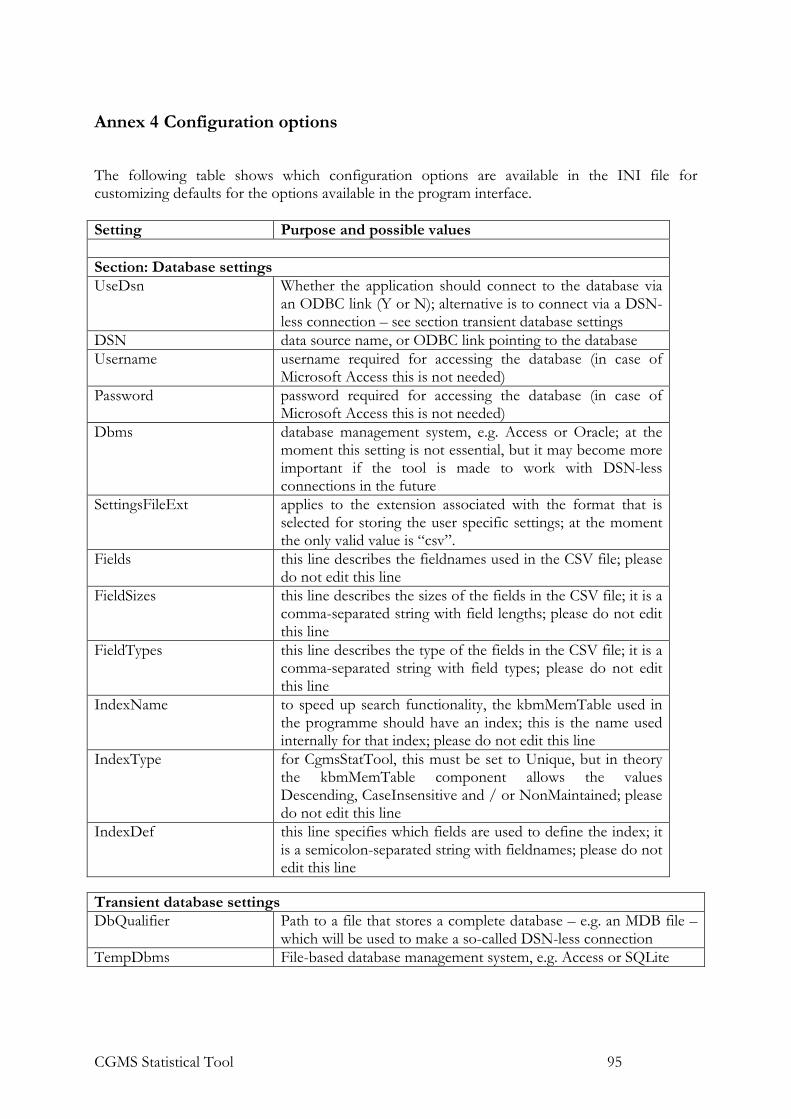
CGMS Statistical Tool 95
Annex 4 Configuration options
The following table shows which configuration options are available in the INI file for customizing defaults for the options available in the program interface. Setting Purpose and possible values Section: Database settings UseDsn Whether the application should connect to the database via
an ODBC link (Y or N); alternative is to connect via a DSN-less connection – see section transient database settings
DSN data source name, or ODBC link pointing to the database Username username required for accessing the database (in case of
Microsoft Access this is not needed) Password password required for accessing the database (in case of
Microsoft Access this is not needed) Dbms database management system, e.g. Access or Oracle; at the
moment this setting is not essential, but it may become more important if the tool is made to work with DSN-less connections in the future
SettingsFileExt applies to the extension associated with the format that is selected for storing the user specific settings; at the moment the only valid value is “csv”.
Fields this line describes the fieldnames used in the CSV file; please do not edit this line
FieldSizes this line describes the sizes of the fields in the CSV file; it is a comma-separated string with field lengths; please do not edit this line
FieldTypes this line describes the type of the fields in the CSV file; it is a comma-separated string with field types; please do not edit this line
IndexName to speed up search functionality, the kbmMemTable used in the programme should have an index; this is the name used internally for that index; please do not edit this line
IndexType for CgmsStatTool, this must be set to Unique, but in theory the kbmMemTable component allows the values Descending, CaseInsensitive and / or NonMaintained; please do not edit this line
IndexDef this line specifies which fields are used to define the index; it is a semicolon-separated string with fieldnames; please do not edit this line
Transient database settings DbQualifier Path to a file that stores a complete database – e.g. an MDB file –
which will be used to make a so-called DSN-less connection TempDbms File-based database management system, e.g. Access or SQLite

CGMS Statistical Tool 96
Section: Default interface settings ShowLogWindow specifies whether or not the log window at the bottom of the
tool interface should be shown at startup (False of True) DefaultSignificanceLevel specifies the default significance level used in particular in the
TimeTrend frame CorrelationFilterValue specifies the lowest correlation that should by default be
shown in the correlation form; the value should of course be in the range 0.0 to 1.0
ModelingMethod specifies whether the SingleFree method should be used by default or rather the BestSubset method
BestModelSelection specifies which summary statistic should be used by default to select the best models; the same statistic will be used to rank the various models
HighlightWrongSign specifies whether the t-values of the indicators should by default be highlighted if they have the wrong sign
HighlightAtSignificance specifies whether the t-values of the terms of the model should by default be highlighted if they are not significant
IndicatorSignificance specifies the level of significance that by default is considered just enough for a term to be meaningful
DisplayBasedOnVif specifies whether models should by default be filtered based on variance inflation factor
MinNumPComps minimum number of Principal Components MinPercOfVar minimum level of variance which is explained by the
components CutoffScore1 first cutoff score CutoffScore2 second cutoff score MinNumSimYears minimum number of similar years MinN minimum number of observations; also needed are
observations pertaining to the target year. MaxNumModelsInCsvFile Maximum number of models that should be saved to a CSV-
file;.default is -1, meaning that there is no maximum Section: Default model settings TrendModelType specifies the default trend model; valid values are: None,
Linear, Quadratic, AutoUpToLinear and AutoUpToQuadratic
TransformYear specifies the default choice whether the years should be transformed; valid values are None and Logarithmic
YearOffset specifies the default offset that is subtracted from the year in case of a logarithmic transformation; also determines the first year the application shows; by default this offset is 1965; it should be reduced for analyses on data dating back further than 1971

CGMS Statistical Tool 97
Section: Default output settings ShrinkingWindowMinimumSize default minimum number of years for fitting a time trend StatsToDisplay indicates which four summary statistics from the file
“statistics.txt” should by default be displayed on the output frame; the line contains a letter for each of the 10 statistics with the letter Y at position x meaning that the x-th statistic should be displayed and the letter N meaning that it should not
MaxVifMeasure specifies the default maximum variance inflation factor beyond which a term should be considered too closely correlated with one of the other terms
MaxNumFreeIndicators default maximum number of free indicators in a model MaxNumModelsInSubset default maximum number of models to be displayed
from a subset DebugLevel parameter which can be varied between 0 and 2 in order
to get less or rather more informational messages, warnings and error messages
MaxWeight weights used for calculating a correction to the time trend in the scenario analysis should not exceed this maximum
Section: Batch settings MinNumAvailYears Minimum number of years, for which indicator values
and yields are available, for calculating regression models.
SecToCloseBatchWindow Seconds before closing the log batch window SaveForecastedYield Indicates whether the prediction resulting from the run
at the actual moment should be stored in the database or not (Y or N)

CGMS Statistical Tool 98
Annex 5 Acronyms and abbreviations
AGRICAB EU FP-7 project to enhance agriculture and forestry planning and management processes in Africa through strengthened Earth Observation (EO) Capacity and better exploitation of satellite data available through GEONETCast
Alterra Wageningen University and Research, Wageningen Environmental Research (Alterra), the Netherlands.
Asemars Actions in Support of the Enlargement of the MARS Crop Yield Forecasting System. The purpose of this project is - among other things - to complete and reinforce the current version of CGMS in order to extend the system thematically and geographically.
Biometris Department of Wageningen University and Research, Wageningen Plant Research, the Netherlands specialised in applied statistics, involved in research as well as education
C++ A powerful, general-purpose, high-level programming language with low-level facilities which has been in use since 1985. It is a multi-paradigm language supporting procedural programming, data abstraction, object-oriented programming and generic programming. It was made an ANSI standard in 1998. Many operating systems were developed using C++ including Windows and Linux. Programmes written in C++ for a specific operating system, can often be ported easily to other platforms.
CGMS Crop Growth Monitoring System, provides the European Commission (DG Agriculture) with objective, timely and quantitative yield forecasts at regional and national scale. CGMS monitors crops development in Europe, driven by meteorological conditions modified by soil characteristics and crop parameters. This mechanistic approach describes crop cycle – e.g. biomass in combination with phenological development from sowing to maturity on a daily time scale. The main characteristic of CGMS lies in its spatialisation component, integrating interpolated meteorological data, soils and crops parameters, through elementary mapping units used for simulation in the crop model.
CSV Comma Separated Values format, is a delimited data format that has fields separated by the comma character and records separated by newlines. Fields that contain a comma, newline, or double quote character, or which start or end with whitespace that is to be preserved, must be enclosed in double quotes. However, if a line contains a single entry which is the empty string, it may be enclosed in double quotes. If a field's value contains a double quote character it is escaped by placing another double quote character next to it. The CSV file format does not require a specific character encoding, byte order, or line terminator format.
DFFITS A statistic which is a scaled measure of the change in the predicted value for the i-th observation. Large absolute values of this statistic for a certain i indicate that thi i-th observation is influential.
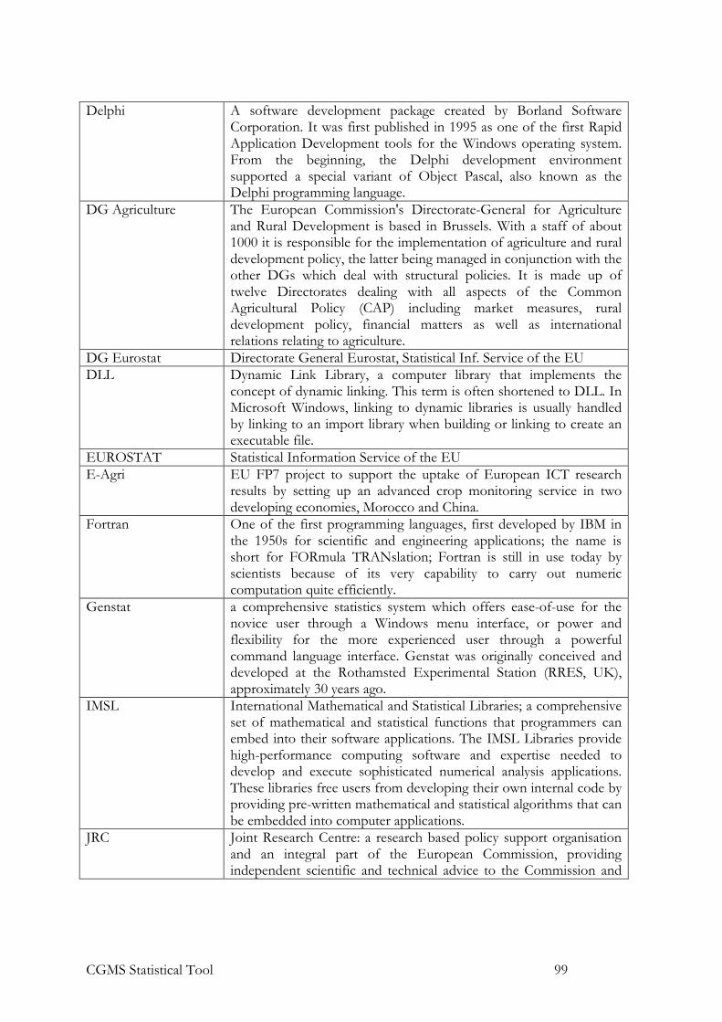
CGMS Statistical Tool 99
Delphi A software development package created by Borland Software Corporation. It was first published in 1995 as one of the first Rapid Application Development tools for the Windows operating system. From the beginning, the Delphi development environment supported a special variant of Object Pascal, also known as the Delphi programming language.
DG Agriculture The European Commission's Directorate-General for Agriculture and Rural Development is based in Brussels. With a staff of about 1000 it is responsible for the implementation of agriculture and rural development policy, the latter being managed in conjunction with the other DGs which deal with structural policies. It is made up of twelve Directorates dealing with all aspects of the Common Agricultural Policy (CAP) including market measures, rural development policy, financial matters as well as international relations relating to agriculture.
DG Eurostat Directorate General Eurostat, Statistical Inf. Service of the EU DLL Dynamic Link Library, a computer library that implements the
concept of dynamic linking. This term is often shortened to DLL. In Microsoft Windows, linking to dynamic libraries is usually handled by linking to an import library when building or linking to create an executable file.
EUROSTAT Statistical Information Service of the EU E-Agri EU FP7 project to support the uptake of European ICT research
results by setting up an advanced crop monitoring service in two developing economies, Morocco and China.
Fortran One of the first programming languages, first developed by IBM in the 1950s for scientific and engineering applications; the name is short for FORmula TRANslation; Fortran is still in use today by scientists because of its very capability to carry out numeric computation quite efficiently.
Genstat a comprehensive statistics system which offers ease-of-use for the novice user through a Windows menu interface, or power and flexibility for the more experienced user through a powerful command language interface. Genstat was originally conceived and developed at the Rothamsted Experimental Station (RRES, UK), approximately 30 years ago.
IMSL International Mathematical and Statistical Libraries; a comprehensive set of mathematical and statistical functions that programmers can embed into their software applications. The IMSL Libraries provide high-performance computing software and expertise needed to develop and execute sophisticated numerical analysis applications. These libraries free users from developing their own internal code by providing pre-written mathematical and statistical algorithms that can be embedded into computer applications.
JRC Joint Research Centre: a research based policy support organisation and an integral part of the European Commission, providing independent scientific and technical advice to the Commission and

CGMS Statistical Tool 100
EU Member States in support of European Union (EU) policies. Main aim is to help to create a safer, cleaner, healthier and more competitive Europe.
MARS Monitoring Agriculture with Remote Sensing, a project started in 1988, initially designed to apply emerging space technologies for providing independent and timely information on crop areas and yields. Since 1993, driven by user requirements, the team has contributed towards a more effective and efficient management of the Common Agricultural Policy through the provision of a broader range of technical support services to DG Agriculture and Member State Administrations.
MARSOP MARS Operational: the project which was carried out by the MARS consortium led by Alterra in the period 2000-2003 and which is now continued in the next term 2004-2008, in order to provide early information on the development and growth conditions of crops.
Mallows Cp A measure of goodness-of-prediction. In general, one should look for models where Mallows Cp is small. A small Cp value indicates that the model is relatively precise (has small variance) in estimating the true regression coefficients and predicting future responses.
MCYFS MARS Crop Yield Forecasting System; was instated as part of the MARS activities to supply the DG Agriculture and EUROSTAT with early information on development, growth conditions and expected yields of crops
NOAA/AVHRR A type of sensor on board of the NOAA satellites, called Advanced Very High Resolution Radiometer; these satellites were operated by a service of the National Oceanic and Atmospheric Administration, U.S.A..
ODBC Open DataBase Connectivity, a standard database access method developed by the SQL Access group in 1992. The goal of ODBC is to make it possible to access any data from any application, regardless of which database management system (DBMS) is handling the data. ODBC manages this by inserting a middle layer, called a database driver, between an application and the DBMS. The purpose of this layer is to translate the application's data queries into commands that the DBMS understands.
R-squared A mathematical term describing how much variation is being explained by the X’s in a regression model. The R-squared value is the fraction of the variance in the data that is explained by a regression model.
RS Remote Sensing: in the broadest sense, this is the measurement or acquisition of information of an object or phenomenon, by a recording device that is not in physical or intimate contact with the object. In practice, remote sensing is the utilization at a distance (as from aircraft, spacecraft, satellite, or ship) of any device for gathering information about the environment. In modern usage, the term usually refers to techniques involving the use of instruments aboard aircraft and spacecraft.

CGMS Statistical Tool 101
S-Plus Platform for statistical analysis. The basis of this platform is the S programming language which was specifically developed for the creation of analytic prototypes. It is an interactive language, allowing statisticians and developers to compare multiple models and share results across systems.
SIGMA EU FP-7 project to develop innovative methods and indicators to monitor and assess progress towards “sustainable agriculture”, focussed on the assessment of longer term impact of agricultural dynamics on the environment and vice versa, in support of GEOGLAM
VIF Variance Inflation Factor. It measures the impact of collinearity among the X's in a regression model on the precision of estimation. It expresses the degree to which collinearity among the predictors degrades the precision of an estimate. Typically a VIF value greater than 10 is of great concern.
WOFOST WOFOST is a mechanistic model that explains crop growth on the basis of the underlying processes, such as photosynthesis and respiration, and how these processes are affected by environmental conditions. The model describes crop growth as biomass accumulation in combination with phenological development. It simulates the crop life cycle from sowing or emergence to maturity. Meteorological data (rain, temperature, wind speed, global radiation, air humidity) are needed as input. Other input data include volumetric soil moisture content at various suction levels, and other data on saturated and unsaturated water flow. Also data on site specific soil and crop management are requested.
CGMS Statistical Tool 102
Annex 6 How to prepare your data for analysis
What is a relational database? The CgmsStatTool works on the basis of a so-called relational database. A database is a structured set of data held in a computer. A database is called relational when extra measures are taken to ensure that relations are maintained between the items of information that are stored in the database. In addition, such databases are normally structured in such a way that redundant data are avoided and unique keys remain unique. A relational database is normally managed by an available database management system (DBMS), consisting of an engine and a graphical user interface (GUI). For the CgmsStatTool, Access was selected as the default DBMS – part of the Microsoft Office suite. Other database management systems may be used instead, but this requires extra configuration. If you want to use a database programme from another office suite, at least you‘ll have to install the database engine (or “driver”) and you’ll probably have to connect via either the ODBC or the JDBC protocol. In view of establishing an appropriate structure, normally a real-world domain is modelled to consist of entities. For each entity a separate table is defined with a number of fields. Each of these fields has a name and - to put it simply - can contain either numerical or text data. Structure of the database
The CgmsStatTool requires a database with a particular structure. The picture below shows the tables that are required, with the relations that exist between them.
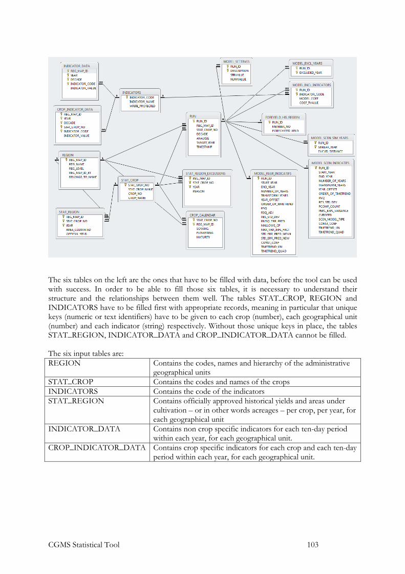
CGMS Statistical Tool 103
The six tables on the left are the ones that have to be filled with data, before the tool can be used with success. In order to be able to fill those six tables, it is necessary to understand their structure and the relationships between them well. The tables STAT_CROP, REGION and INDICATORS have to be filled first with appropriate records, meaning in particular that unique keys (numeric or text identifiers) have to be given to each crop (number), each geographical unit (number) and each indicator (string) respectively. Without those unique keys in place, the tables STAT_REGION, INDICATOR_DATA and CROP_INDICATOR_DATA cannot be filled. The six input tables are: REGION Contains the codes, names and hierarchy of the administrative
geographical units STAT_CROP Contains the codes and names of the crops INDICATORS Contains the code of the indicators STAT_REGION
Contains officially approved historical yields and areas under cultivation – or in other words acreages – per crop, per year, for each geographical unit
INDICATOR_DATA Contains non crop specific indicators for each ten-day period within each year, for each geographical unit.
CROP_INDICATOR_DATA Contains crop specific indicators for each crop and each ten-day period within each year, for each geographical unit.

CGMS Statistical Tool 104
Table REGION An administrative geographical unit is the real-world phenomenon associated with this table. As it is part of a model, the table stores only a few properties of each geographical unit. The structure of the table REGION can be seen more clearly in the picture below:
As far as hierarchy is concerned in the geographical structuring of the area concerned, it is recommended that lower level units – e.g. districts - with similar agro-ecological conditions are grouped together into higher level units – e.g. provinces. Whether this is possible depends of course also on the availability of yield and acreage data for geographical units at those levels.
Once it has been decided how the country will be “broken down” geographically, the table REGION can be filled out. The filling out may be done directly from within the programme Access, or it can be done first in Excel (or another spreadsheet programme). The numbers in the field REG_MAP_ID may be numbered through. That is of course easier done within Excel. If there’s already an existing numbering in place for these units, using those numbers would even be better.
You must start with a record that represents the highest level – e.g. the country – with the field REG_LEVEL equal to zero. Then continue with the next lower level e.g. provinces by inserting the REG_MAP_ID and REG_NAME of the provinces. The hierarchy in the country’s regions is then represented by filling out the fields REG_MAP_ID_BT and BELONGS_TO_NAME of these records - i.e. by inserting the REG_MAP_ID and REG_NAME of the country into those fields. The field REG_LEVEL of those records should be made equal to 1.
Subsequently, the same is done for each of the records at the district level with REG_LEVEL equal to 2. One may continue for deeper levels - where applicable. The picture below shows the table REGION with some data for Senegal in view:

CGMS Statistical Tool 105
After preparation in Excel, one can select, copy and paste the data into the table REGION by right-clicking on the first empty row at the bottom of the table which is marked with an asterisk and by choosing the option “Paste” from the menu that appears – as shown in the picture below:

CGMS Statistical Tool 106
Table STAT_CROP
The structure of the table STAT_CROP can be seen in the picture below:
This table is designed in line with the relational approach; the advantage is that there’s no need to type the name of a crop more than once, so there’s no risk that a typo will cause problems. Furthermore, indexing on the numerical field STAT_CROP_NO allows the DBMS to work faster. The picture below shows the table with some data in view:
Table INDICATORS
The structure of the table INDICATORS can be seen in the picture below:
This table holds the codes and names of indicators. The format of the indicator name is not totally free. The first two characters must contain a string representing a two digit number e.g.

CGMS Statistical Tool 107
‘01’ and should be numbered in a sequential, consecutive order. The program can work with a maximum of indicators.
The column WRITE_PROTECTED can have value ‘Y’ or ‘N’ to avoid that data of indicators are being overwritten when working with data management functionality (see Chapter 13). When using ‘Y’ the data of this indicator is protected. The picture below shows the table with some data in view:
Table STAT_REGION
A set of yield observations for a certain crop, in a particular administrative geographical unit in a particular year is the real-world phenomenon associated with this table. The most important property that is stored in the table is the official yield, which implies that the figure was officially approved. In addition the area cultivated with that crop within that geographical area is added as property, but it is not essential to fill out that column for the CgmsStatTool to work.
The structure of this table is shown below:
The field REG_MAP_ID refers to the field with the same ID-value in table REGION and the field STAT_CROP_NO to the field with the same ID-value in table STAT_CROP. Only ID-values that already occur in the table REGION can be used as REG_MAP_ID here. And similarly: only ID-values that already occur in table STAT_CROP can be used as STAT_CROP_NO here.
For filling out this table, it is definitely recommended to use Excel (or another spreadsheet programme). Assuming that the data were provided in an electronic form and can be opened / imported into Excel: names of regions and / or crops may have to be replaced by numbers. In that case, the data can first be sorted by region. Then an extra column can be inserted next to the existing column for region and filled with the appropriate numbers for each region. This can be

CGMS Statistical Tool 108
done e.g. by copying a number to a whole block of cells in that column. Afterwards, the data can be sorted by crop and an extra column can be inserted for crop too etc.
Other conversions can be done too by adding extra columns. In the end, the columns with the correctly formatted data can all be moved to one side and copied as a block into the database table - as shown above with the columns correctly sorted. For the DBMS, it does not matter how the rows - or records - are sorted. It is good practice to save the spreadsheet for these conversions, as evidence that the conversions were carried out correctly.
If the area under cultivation is not known for a particular area, crop and year, then the field must be left blank. The same is true for the official yield. To fill out 0.0 in such a case is wrong and it will cause problems when one tries to do an analysis with the CgmsStatTool later on. In general, a period of 6 years is considered minimal for carrying out a meaningful analysis with the tool.
Table INDICATOR_DATA The structure of this table is shown below:
As is the case with table STAT_REGION, the field REG_MAP_ID refers to the field with the same ID-value in table REGION and the field INDICATOR_CODE to the field with the same ID-value in table INDICATORS. Only ID-values that already occur in the table REGION can be used as REG_MAP_ID here. And similarly: only ID-values that already occur in table INDICATORS can be used as INDICATOR_CODE here. It is assumed that the concept of dekads - or in other words ten-day periods – is known. The values in the field DECADE can range from 1 to 36.
The table is used to store both historical data as well as data collected so far for the growing season that is in progress. In the case of regression analysis, the historical data are needed for the analysis and the data for the current growing season are used for prediction. In the case of scenario analysis, historical and recent data are used only for the analysis.
This table is used to store values of different kinds of indicators that are not crop specific: • Remote sensing derived indicators – e.g. vegetation indices, indices for photosynthetic
absorption, indices for soil moisture, • Meteorological indicators – e.g. the amount of rainfall since a certain date. • Etc.

CGMS Statistical Tool 109
Table CROP_INDICATOR_DATA The structure of this table is shown below:
As is the case with table STAT_REGION, the field REG_MAP_ID refers to the field with the same ID-value in table REGION, the field STAT_CROP_NO to the field with the same ID-value in table STAT_CROP and the field INDICATOR_CODE to the field with the same ID-value in table INDICATORS. Only ID-values that already occur in the table REGION can be used as REG_MAP_ID here. And similarly: only ID-values that already occur in table STAT_CROP can be used as STAT_CROP_NO here. And similarly: only ID-values that already occur in table INDICATORS can be used as INDICATOR_CODE here
This table is used to store values of different kinds of indicators for one specific crop for instance results from crop growth model simulations (e.g. WOFOST) or NDVI values that have been spatially aggregated to regions according a crop specific mask like irrigated rice.

CGMS Statistical Tool 110
Troubleshooting in relation to entered / available data
All input information that the CgmsStatTool can show and process is derived from the database. As explained, often records in one table can only exist in that table because a record with a unique ID used in that record exists in another table. And if strictly speaking there’s no such dependency in the database, still the programme may sometimes suppose certain records to be there. E.g. the programme may start with an error message, as shown below:
This error message can be understood if one knows that in table REGION a country is defined by an entry with REG_LEVEL equal to zero. If no such entry has been defined in that table, then the programme cannot retrieve further information, shows the above dialog and upon OK it opens with an empty screen.
Other problems with data in table REGION should be easy to diagnose. If the list box for “Area” does not show the hierarchy in the regions properly, then it can’t be too difficult to understand what is wrong with the data in table REGION.
In general, error messages and warnings are shown in the memo window. By default, this memo window is hidden. Whenever it is relevant, the programme will suggest to make it visible:
When the user clicks “Yes”, then the memo field at the bottom of the main window is made visible. The memo field is shown in the screenshot below with a red frame drawn around it. The memo field can be shown or hidden at any time, by selecting “View” from the menu and checking or unchecking the option “Log Window”. It is recommended to keep an eye on the messages appearing there whilst working with the CGMS Statistical Tool.
Not all problematic states of the database are reported by means of error messages and warnings. If the drop-down box for crops is completely empty, then it might be due to table STAT_CROP being empty. If however there are entries in the table STAT_CROP, the drop-down box might still be empty due to the fact that there are no crop statistics in the table STAT_REGION for the

CGMS Statistical Tool 111
selected region at all. This is normally reported by means of a warning: “No crop statistics available for this area”.
The table STAT_REGION may contains some data, and the name of the crop may appear in the list. However, a dataset with yield observations for e.g. only 4 years is considered too minimal for an analysis. If the tables REGION, STAT_CROP and STAT_REGION are all properly filled with enough data, then the user should be able to carry out time trend analyses.
Crop statistics may not be available at all levels of the hierarchy. If crop statistics are available at lower levels only – e.g. for districts – then the user may aggregate data to provincial level. Of course an officially approved algorithm should be used for this. The field AREA_CULTIVATED in table STAT_REGION might be needed for that algorithm.
Likewise, if data are lacking in the tables CROP_INDICATOR_DATA and INDICATOR_DATA, the user may experience difficulties with regression and scenario analysis. For higher levels in the hierarchy, it may be necessary to aggregate indicator data to higher levels. Also in this case, a well-considered algorithm should be used to do so.
Crop indicators are not always generated for all the dekads in the year. Obviously, a crop indicator like “leaf area index” (LAI) has no value for a great part of the year. In general, no records are entered for those dekads. When the programme does not find entries for a particular indicator for the selected dekad, then that indicator is not shown. In other words: for a crop indicator to appear in the list box with “available indicators”, a dekad should be selected within the growing season of the selected crop. And it makes no sense e.g. to look for “sum of rainfall” (SOR) for dekad 12 (end of April) if that indicator is calculated as cumulative rainfall from May 1 onwards. Note that the data management tool (see Chapter 13) supports the user in using data, linked to a certain dekad, for other dekads in setting up regression or scenario models.
For prediction models to work, indicator values are always needed for the current year. Crop yield forecasting is preferably done on a near real-time basis. However, it might be difficult to get hold of the values for the current dekad or at least for a recent dekad. So sometimes, the value for a particular indicator might not yet be available. In that case, the programme will generate a warning: “Indicator with code XYZ was not shown, because there is no value for it for the target year”. It means that that indicator could be included in a regression model, but with that model it would not be possible to make a forecast. In this case the user can enable the calibration mode.
Other tables So far only 6 tables from the database have been discussed. As mentioned, they need to be filled with data i.e. essential input for the CgmsStatTool. All other tables are filled by the tool (in other words the programme). Those other tables in the database are used to store workflow information in the database – i.e. when a model is saved on one of the Output tab sheets. This workflow information consists of selected inputs, particulars that can help to identify the run as well as of obtained summary results. In the first place the tables RUN, FOREYIELD_HIS_REGION, MODEL_SETTINGS, MODEL_EXCL_YEARS and MODEL_INCL_INDICATORS are used to store this information. Furthermore - depending on the type of analysis - either the table MODEL_REGR_INDICATIFS is used (regression analysis) or the tables MODEL_SCEN INDICATIFS and MODEL_SCEN_SIM_YEARS

CGMS Statistical Tool 112
(scenario analysis). The workflow information is displayed in a summarised form on the Saved Model tabsheets.


![Agency, version?, Date 2014? [update filed in the slide master] Coordination Group for Meteorological Satellites - CGMS Add CGMS agency logo here (in the](https://img.pdfslide.us/doc/110x75/56649c935503460f9494e678/agency-version-date-2014-update-filed-in-the-slide-master-coordination.jpg)