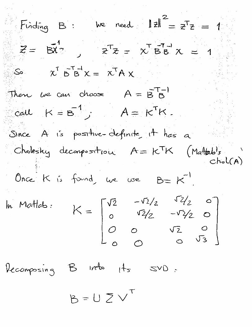
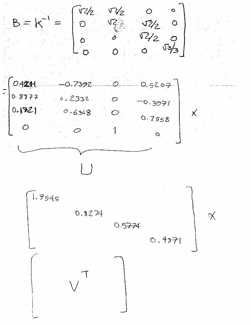
V 1=[0.42710.88770.17210.0000

]V 2=[−0.73290.23320.63180.0000

]V 3=[0.00000.00000.00001.0000

]V 4=[0.5207

−0.39710.75580.0000

]The U vectors that map to these V vectors from the unit 4-sphere after applying the transformation are:

U 1=[0.74940.65970.05660.0000

]U 2=[−0.61160.65690.44090.0000

]U 3=[0.00000.00000.00001.0000

]U4=[0.2536

−0.36500.89580.0000

]Problem 2

Determine the Jacobian (velocity and angular velocity) for the cylindrical manipulator of HW2 in symbolic form, referring to the wrist center. Symbolic solution with MATLAB highly suggested.

Cylindrical base

The cylindrical manipulator from homework 2:

% Define constants and symbolsh = 1;d = 2;syms q1 q2 q3;q = [q1;q2;q3]; % Define the links and robotLink = sym(zeros(4,4,3));Link(:,:,1) = RotationMatrix(3, q1) *TranslationMatrix([0 0 h]); % Cylindrical baseLink(:,:,2) = TranslationMatrix([0 0 q2])*RotationMatrix(1, -pi/2) ;Link(:,:,3) = TranslationMatrix([0 0 q3]);Robot = mprod(Link,3); % Custom function; right-side matrix product along dimension 3 % Determine the Jacobian matricesJv = jacobian(Robot(1:3,4),q); z = squeeze(Link(1:3,3,:));Jw = z .* repmat([1 0 0],3,1);J = [Jv;Jw];

We calculate the velocity Jacobian using the definition: partial derivative of the position vector with respect to each joint angle (MATLAB has a function built in for this). We also calculate the angular velocity Jacobian matrix using the short cut defined in class (using the third column of the rotation matrix, called z in our notes and here). We then combine these into a single Jacobian matrix.

J=[−q3 c1 0 −s1−q3 s1 0 c10 1 00 0 00 0 01 0 0

]Page 3 of 10

Solutions to Problem 2 and forward by CurtLaubscher

Whole robot

There was some confusion exactly what portion of the robot we needed the Jacobian of; here I do the same thing but applied to the whole robot.

% Define constants and symbolsh = 1;d = sym('d6');syms q1 q2 q3 q4 q5 q6;%q = [q1;q2;q3;q4;q5;q6]; % Define the links and robotLink = sym(zeros(4,4,6));Link(:,:,1) = RotationMatrix(3, q1) *TranslationMatrix([0 0 h]); % Cylindrical baseLink(:,:,2) = TranslationMatrix([0 0 q2])*RotationMatrix(1, -pi/2) ;Link(:,:,3) = TranslationMatrix([0 0 q3]);Link(:,:,4) = RotationMatrix(3, q4) *RotationMatrix(1, -pi/2) ; % Spherical wristLink(:,:,5) = RotationMatrix(3, q5) *RotationMatrix(1, pi/2) ;Link(:,:,6) = RotationMatrix(3, q6) *TranslationMatrix([0 0 d]);Robot = mprod(Link,3); % Custom function; right-side matrix product along dimension 3CumLink = cummprod(Link,3); % Cumulative mprod along dimension 3 % Determine the Jacobian matricesr%Jv = jacobian(Robot(1:3,4),q); % This method agrees with Jv calculated belowz = remdim(CumLink(1:3,3,:),2); z = [[0;0;1] z(:,1:end-1)]; % Offset by 1o = remdim(CumLink(1:3,4,:),2); o = [zeros(3,1) o(:,1:end-1)]; % Offset by 1Jv = ... % I calculate Jv using the method shown in the notes here cross(z, repmat(Robot(1:3,4,:),1,size(Link,3))-o).*repmat([1 0 0 1 1 1],3,1) ... +z.*(1-repmat([1 0 0 1 1 1],3,1));Jw = z .* repmat([1 0 0 1 1 1],3,1);J = simplify([Jv;Jw]);

The velocity Jacobian was calculated using the method described in the notes in this case, which wast tested and it returns the same thing as using the jacobian function. The Jacobian matrix is found:

J=[−d6(c1 c5+c4 s1 s5)−q3 c1 0 −s1 −d6 c1 s4 s5 d6(s1 s5+c1c4 c5) 0−d6(c5 s1−c1 c4 s5)−q3 s1 0 c1 −d6 s1 s4 s5 d6(c4 c5 s1−c1 s5) 0

0 1 0 −d6 c4 s5 −d6 c5 s4 00 0 0 −s1 −c1 s4 c1 c4 s5−c5 s10 0 0 c1 −s1s4 c1 c5+c4 s1 s51 0 0 0 −c4 −s4 s5

]Problem 3

For the 3×3 linear velocity Jacobian above, find all singularities and provide a graphical interpretation. What is the rank of the 3×3 angular velocity Jacobian? Provide an interpretation.

Here we consider the cylnidrical base, which has a 3×3 linear and angular velocity Jacobian matrices.

Jv_det = simplify(det(Jv)); % Result: q3Jv_rank = rank(Jv); % Result: 3Jw_rank = rank(Jw); % Result: 1

Singularities occur when q3 = 0, the only solution to the determinant of the velocity Jacobian matrix being zero. Graphical interpretation: This makes sense because this variable represents radial offset

Page 4 of 10

from the central axis of the robot, and we know a radius of zero is a special point. If we rotate q1 when q3 is zero, we know no velocity is produced at the point of interest.

The rank of the angular velocity Jacobian matrix is 1. Mathematically, this means we have only a singleindependent vector. Physically, this is because q1 is the only variable that can produce a rotation since itis a revolute joint; the other two variables q2 and q3 apply to prismatic joints, which are incapable of producing rotation by themselves.

Problem 4

For the 2-link planar manipulator, prove that Yoshikawa's manipulability measure is independent of the first joint coordinate (consider the 2×2 linear velocity Jacobian only).

% Define symbolicsL = [sym('L1', 'positive'); sym('L2', 'positive')];q = [sym('q1', 'real'); sym('q2', 'real' )];

% Define links and robotLink = sym(zeros(4,4,2));Link(:,:,1) = RotationMatrix(3, q(1)) * TranslationMatrix([L(1);0;0]);Link(:,:,2) = RotationMatrix(3, q(2)) * TranslationMatrix([L(2);0;0]);Robot = mprod(Link,3);

% CumLink% CumLink = sym(zeros(4,4,2));% CumLink(:,:,1) = Link(:,:,1);% CumLink(:,:,2) = Link(:,:,1)*Link(:,:,2);CumLink = cummprod(Link,3); % Custom function; cumulative mprod; equivalent to above

% Calculate Jacobian matricesz = remdim(CumLink(1:3,3,:),2); z = [[0;0;1] z(:,1:end-1)]; % Offset by 1o = remdim(CumLink(1:3,4,:),2); o = [zeros(3,1) o(:,1:end-1)]; % Offset by 1on = Robot(1:3,4,:);Jv = cross(z, repmat(on,1,2) - o);Jw = z;Jv = Jv(1:2,:); Jw = Jw(1:2,:); % Convert to two-dimensionalJ = [Jv;Jw];

% Calculate manipulabilitymu = simplify(sqrt(det(J.'*J)));

We see that μ is only a function of q2; it is independent of q1.

Problem 5

For the 2-link planar manipulator, plot the manipulability ellipses (planar velocity only) at a few values of q2 for q1 = 0. Take link lengths equal to 1. Determine the “best” value of q2 visually.

% Define some parametersscale = 0.15; % Ellipse scaleL1 = 1; % Link 1 lengthL2 = 1; % Link 2 length % Do length substitutions Point1 = subs(CumLink(:,:,1),L,[L1;L2]); Point2 = subs(CumLink(:,:,2),L,[L1;L2]);Robot2 = subs(Robot, L,[L1;L2]);Jv2 = subs(Jv, L,[L1;L2]);

Page 5 of 10

μ=L1L2|sin q2|

% Generate q dataN = 12;q1 = 0;q2 = linspace(-pi, pi, N+1); q2=q2(1:end-1); % Generate unit circlet = linspace(-pi, pi, 20);u = [cos(t) ; sin(t)]; % Plotfigure();set(gcf, 'color', [1 1 1]);hold('on');axis square;xlim([-0.5 2.5]);for k = 1 : N % Find points of interest on the ellipse c = double(subs(Robot2, q, [q1;q2(k)])); c = c(1:3,4); p0 = [0;0;0]; p1 = double(subs(Point1, q, [q1;q2(k)])); p1 = p1(1:3,4); p2 = double(subs(Point2, q, [q1;q2(k)])); p2 = p2(1:3,4); p = [p0 p1 p2]; % Create ellipse points Jv2s = double(subs(Jv2,q,[q1;q2(k)])); v = zeros(size(u)); for n = 1 : length(t) v(:,n) = Jv2s*u(:,n); end % Find the ellipse axes [U,S,V] = svd(Jv2s); Vmax = Jv2s*V(:,1); Vmin = Jv2s*V(:,2); % Plot robot, ellipse, and ellipse axes plot(p(1,:), p(2,:), 'k.-'); plot(c(1) + scale*v(1,:), c(2) + scale*v(2,:), 'b'); plot(c(1) + scale*Vmax(1)*[-1 1], c(2) + scale*Vmax(2)*[-1 1], 'r-'); plot(c(1) + scale*Vmin(1)*[-1 1], c(2) + scale*Vmin(2)*[-1 1], 'r-'); end

Page 6 of 10

Looking at this figure, eyeballing for the largest area of an ellipse, it looks like when the second link is in one of the two vertical positions (q2 is ±π/2), we have maximum manipulability. Smaller q2 appear tobe thinner, while larger appear to be shorter.

Problem 6

Assuming the statement in Problem 4 is true, find the value of q2 maximizing μ analytically. What is μ'smaximum value?

% Substitute lengthsmu2 = subs(mu, L, [L1;L2]); % Add the last pointq2b = [q2 pi]; % Substitute q value into mu formulamu3 = double(subs(mu2, q(2), q2b)); % Plotfigure();set(gcf, 'color', [1 1 1]);plot(q2b, mu3);xlabel('q_2');ylabel('\mu');

Page 7 of 10

Just by looking at the plot, it looks like the maximum is at the suspected ±/2. The value of μ is 1 at these points.

% Find the maximum symbolicallydmu2 = diff(mu2, q(2));

To symbolically determine the maxumum, we take the derivative with respect to q2, and set it equal to zero. This is satisfied only in the case when the sine of q2 is zero, or the cosine of q2 is zero; i.e. ∀n ,∈ℤ

q2 = 2πn/4. We can show that at only for n=±1 (when restricting ourselves from −π to π) this is a maximum by taking the second derivative and checking it is negative, though this won't help with the discontinuous points; we can use intuition when looking at the plot to not formally/rigorously see that the maximums are correct.

Note that when considering physical capabilities, the arm cannot go underground; only one of these answers is physically possible.

Functions

Throughout this document, some functions are defined which may be unclear. They are defined here.

mprod: matrix productfunction out = mprod(M,dim,direction) % Default argument for direction is 'right' if (nargin < 3) direction = 'right'; end

Page 8 of 10

∂μ

∂q2=sgn (sin (q2))cos (q2)

% Create indexing cells S = cell(ndims(M),1); for j = 1 : ndims(M) if (j == dim) S{j} = 0; else S{j} = ':'; end end % Determine the output size outsize = size(M); outsize = [outsize(1:dim-1) outsize(dim+1:end)]; out = eye(outsize); % Calculate output for k = 1 : size(M,dim) S{dim} = k; Mk = subsref(M, struct('type', '()', 'subs', {S})); Mk = remdim(Mk, dim); if (strcmp(direction,'right')) out = out*Mk; elseif (strcmp(direction,'left')) out = Mk*out; else error('Invalid direction.'); end end end

cummprod: cumulative matrix productfunction out = cummprod(M,dim,direction) % Default argument for direction is 'right' if (nargin < 3) direction = 'right'; end % Create indexing cells S = cell(ndims(M),1); for j = 1 : ndims(M) if (j == dim) S{j} = 0; else S{j} = ':'; end end % Determine the output size out = zeros(size(M)); % Calculate output sizes = size(M); sizes = [sizes(1:dim-1) sizes(dim+1:end)]; last = eye(sizes); for k = 1 : size(M,dim) S{dim} = k; Mk = subsref(M, struct('type', '()', 'subs', {S})); Mk = remdim(Mk, dim); if (strcmp(direction,'right')) last = last*Mk; elseif (strcmp(direction,'left')) last = Mk*last; else error('Invalid direction.'); end out = subsasgn(out, struct('type', '()', 'subs', {S}), last); end

Page 9 of 10

end

remdim: remove dimensionfunction out = remdim(M, dim, index) if (nargin < 2) dim = ndims(M); end if (nargin < 3) index = 1; end if (length(dim) == 1) outsize = size(M); outsize = [outsize(1:dim-1) outsize(dim+1:end)]; S = cell(ndims(M),1); for j = 1 : ndims(M) if (j == dim) S{j} = index; else S{j} = ':'; end end Msub = subsref(M, struct('type', '()', 'subs', {S})); out = reshape(Msub, outsize); else out = M; for k = 1 : length(dim) out = remdim(out, dim(k)); end endend

Page 10 of 10