Embed Size (px)
Citation preview
The Causal Effects of Education
on Earnings and Health∗
James J. HeckmanUniversity of Chicago
and the American Bar Foundation
John Eric HumphriesUniversity of Chicago
Gregory VeramendiArizona State University
March 12, 2015
∗James Heckman: Department of Economics, University of Chicago, 1126 East 59th Street, Chicago, IL60637; phone: 773-702-0634; fax: 773-702-8490; email: [email protected]. John Eric Humphries: Departmentof Economics, University of Chicago, 1126 East 59th Street, Chicago, IL 60637; phone: 773-980-6575; email:[email protected]. Gregory Veramendi: Arizona State University, 501 East Orange Street, CPCOM412A, Tempe, AZ 85287-9801; phone: 480-965-0894; email: [email protected]. This paper waspresented at the Becker Friedman Institute conference in honor of Gary Becker, October 30, 2014. It wasalso presented as the Sandmo Lecture at the Norwegian School of Economics, January 13, 2015. We thankChris Taber for insightful comments. We also thank Ariel Pakes and other participants at a Harvard LaborEconomics Workshop April, 2014, for helpful comments on a previous draft. We thank Eleanor Dillon andMathew Wiswall for comments on this draft received at a seminar at Arizona State University, February, 2015.This research was supported in part by: the American Bar Foundation; the Pritzker Children’s Initiative; theBuffett Early Childhood Fund; NIH grants NICHD R37HD065072 and NICHD R01HD54702; an anonymousfunder; Successful Pathways from School to Work, an initiative of the University of Chicago’s Committee onEducation funded by the Hymen Milgrom Supporting Organization; and the Human Capital and EconomicOpportunity Global Working Group, an initiative of the Center for the Economics of Human Development,affiliated with the Becker Friedman Institute for Research in Economics, and funded by the Institute forNew Economic Thinking. Humphries acknowledges the support of a National Science Foundation GraduateResearch Fellowship. The views expressed in this paper are solely those of the authors and do not necessarilyrepresent those of the funders or the official views of the National Institutes of Health. The Web Appendixfor this paper is https://heckman.uchicago.edu/eff-ed-earn-health.
1

The Causal Effects of Education on Earnings and Health March 12, 2015
Abstract
This paper estimates a robust dynamic model of the causal effects of differentlevels of schooling on earnings and health. Our framework synthesizes approachesused in the dynamic discrete choice literature with approaches used in the reducedform treatment effect literature. We estimate economically interpretable and policyrelevant treatment effects and interpret the economic content of instrumental variablesestimators. Cognitive and noncognitive endowments play important roles in explainingobserved differences in earnings and health across education levels. Nonetheless, aftercontrolling for them, there are substantial causal effects of education at all stages ofschooling. Continuation values associated with dynamic sequential schooling choicesare empirically important components of estimated causal effects. There is considerableheterogeneity in the effects of schooling on outcomes at different schooling levels and inthese effects across persons. We find strong sorting on gains consistent with comparativeadvantage, but only at higher levels of schooling. This result is not imposed in ourestimation procedure. We find that the estimated causal effects of education varywith the level of cognitive and noncognitive endowments. Estimates of causal effectsusing standard instrumental variables are often quite different from the economicallyinterpretable and policy relevant treatment effects derived from our model.
Keywords: education, earnings, health, rates of return, causal effects of education
JEL codes: C32, C38, I12, I14, I21
James Heckman John Eric HumphriesDepartment of Economics Department of EconomicsUniversity of Chicago University of Chicago1126 East 59th Street 1126 East 59th StreetChicago, IL 60637 Chicago, IL 60637Phone: 773-702-0634 Phone: 773-980-6575Email: [email protected] Email: [email protected]
Gregory VeramendiDepartment of EconomicsArizona State University501 East Orange Street, CPCOM412ATempe, AZ 85287-9801Phone: 480-965-0894Email: [email protected]
2
The Causal Effects of Education on Earnings and Health March 12, 2015
1 Introduction
In his pioneering research on human capital, Gary Becker (1962; 1964) identified the rate
of return to education as a central policy parameter. He launched an active industry on
estimating rates of return.1
Becker focused on internal rates of return that equate the discounted values of the
earnings streams associated with different levels of education. He noted that the full return
to schooling also includes nonmarket benefits and nonpecuniary costs. Individuals should
continue schooling as long as their marginal internal rate of return exceeds their marginal
opportunity cost of funds. If the social return exceeds the social opportunity cost of funds,
there is aggregate under-investment in education.
Formidable challenges are faced in estimating internal rates of return: (a) lifetime earnings
profiles are required; (b) observed earnings profiles are subject to selection bias; and (c)
quantifying nonmarket benefits and nonpecuniary costs is a difficult task. In a neglected paper,
Becker and Chiswick (1966) addressed challenge (a) and developed a tractable framework for
measuring rates of return to schooling that utilizes cross-section synthetic cohort data on
earnings to approximate life cycle earnings data. Mincer (1974) improved on this model by
adding work experience. The “Mincer Equation” has become the workhorse of the empirical
literature on estimating rates of return:
lnY (Si, Xi) = αi + ρi Si︸︷︷︸years of
schooling
+φ( Xi︸︷︷︸work
experience
) (1)
where Y (Si, Xi) is the earnings of individual i with Si years of schooling and work experience
Xi, αi is an “ability to earn” parameter that is common across all schooling levels and ρi is
the “rate of return” to schooling for person i that is assumed to vary among individuals.
Equation (1) and its variants have become the standard framework for estimating rates
1For surveys of this literature, see, e.g., Card (1999, 2001); Heckman, Lochner, and Todd (2006);Oreopoulos and Salvanes (2011); McMahon (2009), and Oreopoulos and Petronijevic (2013).
3
The Causal Effects of Education on Earnings and Health March 12, 2015
of return.2 While ρi is not, in general, an internal rate of return for individual i, it is the
causal effect of an increase in one year of schooling on log earnings from any base state of
schooling holding αi and Xi fixed.3
ρi ignores the continuation values arising from the dynamic sequential nature of the
schooling decision where information is updated and schooling at one stage opens up options
for schooling at later stages.4 The distribution of ρi and its correlation with Si have become
central targets of empirical studies of the causal effects of education. A positive correlation is
consistent with a meritocratic society. People who benefit from schooling get more of it. A
negative correlation indicates problems with access to schooling.
Two approaches have been developed to address challenge (b) and estimate rates of
return in the general case where ρi is correlated with Si (sorting bias) and Si is correlated
with αi (ability bias). They are: (I) structural models that jointly analyze outcomes and
schooling choices,5 and (II) treatment effect models that use instrumental variables methods
(including randomization and regression discontinuity methods) as well as matching on
observed variables to identify “causal parameters.”6
The structural approach explicitly models agent decision rules. It uses a variety of
sources of identification including exclusion restrictions (instrumental variables), conditional
independence assumptions on unobservables and functional form assumptions (see, e.g.,
Blevins, 2014). The final two sources of identification are often controversial. The structural
approach identifies the margins of choice identified by instruments and can evaluate the
impacts of different policies never previously implemented.
The instrumental variable approach is agnostic about agent decision rules and relies solely
2See, e.g., Cutler and Lleras-Muney (2010) who apply model (1) to estimate the causal effect of educationon health.
3The stringent conditions under which ρi is an internal rate of return and evidence that they are notsatisfied in many commonly used samples are presented in Heckman, Lochner, and Todd (2006).
4Weisbrod (1962) first raised this point. There is later work by e.g., Comay, Melnik, and Pollatschek(1973); Altonji (1993); Cameron and Heckman (1993), and Eisenhauer, Heckman, and Mosso (2015).
5See e.g., Willis and Rosen (1979); Keane and Wolpin (1997); Eisenhauer, Heckman, and Mosso (2015).6See, e.g., Angrist and Imbens (1995); Angrist and Pischke (2009) for IV, and Heckman, Ichimura, and
Todd (1998).
4
The Causal Effects of Education on Earnings and Health March 12, 2015
on exclusion restrictions to identify its estimands. This approach is often more transparent in
securing identification than is the structural approach. However, the economic interpretation
of its estimands is often obscure. In a model with multiple levels of schooling, LATE often does
not identify the separate margins of choice traced out by instruments or the subpopulations
affected by them. Its estimands are irrelevant for addressing policy questions except when
the variation induced by the instruments corresponds closely to variation induced by the
policies of interest.7
This paper develops and applies a methodology that offers a middle ground between the
reduced form treatment approach and the fully structural dynamic discrete choice approach.
Like the structural literature, we estimate causal effects at clearly identified margins of choice.
Our methodology identifies which agents are affected by instruments as well as which agents
would be affected by alternative policies never previously implemented. Like the treatment
effect literature, we are agnostic about the precise rules used by agents to make decisions.
Unlike that literature, we recognize the possibility that people somehow make decisions and
account for the consequences of their choices. We approximate agent decision rules and do
not impose the cross-equation restrictions that are the hallmark of the structural approach.8
Using a generalized Roy framework, we estimate a multistage sequential model of educa-
tional choices and their consequences.9 An important feature of our model is that educational
choices at one stage open up educational options at later stages. Each educational decision is
approximated using a reduced form discrete choice model. The anticipated consequences of
future choices and their costs are implicitly valued by individuals when deciding whether or
not to continue their schooling. Our model approximates a dynamic discrete choice model
7See Heckman (2010).8Such approximations are discussed in Heckman (1981), Eckstein and Wolpin (1989), Cameron and
Heckman (2001), and Geweke and Keane (2001).9Our approach is related to the analyses of Heckman and Vytlacil (1999, 2005, 2007a,b), Carneiro,
Heckman, and Vytlacil (2010, 2011), and Eisenhauer, Heckman, and Vytlacil (2015), who introduce choicetheory into the instrumental variables literature. They focus their analysis on binary choice models but alsoanalyze ordered and unordered choice models with multiple outcomes to estimate economically interpretabletreatment effects. Expanding on that body of research, we consider multiple sources of identification besidesinstrumental variables, and link our analysis more closely than they do to the dynamic discrete choiceliterature.
5

The Causal Effects of Education on Earnings and Health March 12, 2015
without taking a stance on exactly what agents are maximizing or how their information sets
are being updated.
Like structural models, our model is identified though multiple sources of variation.
Drawing from the matching literature, we identify the causal effects of schooling at different
stages of the life cycle by using a rich set of observed variables and by proxying unobserved
endowments. Unlike previous work on matching, we correct our proxies for measurement
error and the bias introduced into the measurements by family background. We can also
use exclusion restrictions to identify our model as in the IV and control function literatures.
Unlike many structural models, we provide explicit proofs of model identification.
Our framework allows for ex-ante valuations as in dynamic discrete choice models but
does not explicitly identify them.10 However, we can estimate ex-post returns to schooling,
and model how they depend on both observed and unobserved variables. We decompose the
ex-post treatment effects into (a) the direct benefits of going from one level of schooling to
the next11 and (b) continuation values arising from access to additional education beyond
the immediate next step.
Estimating our model on NLSY79 data, we investigate foundational issues in human
capital theory. We report the following findings. (1) Ability bias accounts for a substantial
portion (ranging between a third and two-thirds) of the raw differences in outcomes classified
by education. At the same time, there are substantial causal effects of education on earnings
and health.12 (2) Estimated causal effects differ by schooling level and depend on observed
and unobserved characteristics of individuals. While the returns to high school are roughly
the same across endowment levels, only high-endowment individuals benefit from college
graduation. There is positive sorting on gains (“sorting bias” or “pursuit of comparative
advantage”) only at higher educational levels, but there is sorting into schooling based on
10See, e.g., Eisenhauer, Heckman, and Mosso (2015), where this is done.11The human capital literature traditionally focused on the direct causal benefits of one final schooling
level compared to another, but makes sequential comparisons from the lowest levels of schooling to the highest(Becker, 1964)
12This finding runs counter to a common interpretation in the literature based on comparing IV and OLSestimates of Equation (1). See, e.g., Griliches (1977) and Card (1999, 2001).
6
The Causal Effects of Education on Earnings and Health March 12, 2015
observed and unobserved variables in earnings equations across all schooling levels (“ability
bias”).
(3) The early literature ignored the dynamics of schooling decisions. We find that
continuation values arising from sequential choices are empirically important. Continuation
values depend on cognitive and noncognitive endowments. Low endowment individuals gain
mostly from the direct effect of high school graduation while high endowment individuals
gain mostly in terms of continuation values. Low endowment individuals do not benefit from
graduating college.
(4) Our schooling choice model is consistent with a variety of decision rules and allows for
time inconsistency, regret and systematic mistakes due to cognitive failures. We use model
estimates to test the assumptions of forward looking behavior and selection on gains often
assumed in estimating dynamic discrete choice models.13 We find that agents do not know,
or act on, publicly available information on college tuition costs in making decisions about
graduating high school. Nonetheless, agents sort into schooling on ex-post gains, especially
at higher schooling levels. A core tenet of human capital theory is thus confirmed.
(5) Our evidence of sorting into schooling on gains that varies across schooling levels does
not support the Mincer model (1). The distributions of annualized gains vary greatly across
schooling levels.
(6) Our paper contributes to an emerging literature on the importance of both cognitive and
noncognitive endowments in shaping life outcomes.14 Consistent with the recent literature, we
find that both cognitive and noncognitive endowments are important predictors of educational
attainment. Within schooling levels, cognitive and noncognitive endowments have additional
impacts on most outcomes.15
(7) We meet challenge (c) and estimate substantial causal effects of education on health
13See e.g., Rust (1994); Keane and Wolpin (1997); Blevins (2014).14See, e.g., Borghans, Duckworth, Heckman, and ter Weel (2008); Heckman, Stixrud, and Urzua (2006);
Almlund, Duckworth, Heckman, and Kautz (2011).15Our estimates of the causal effects of education do not require that we separately isolate the effects of
individual cognitive and noncognitive endowments on outcomes, just that we control for them as a set.
7
The Causal Effects of Education on Earnings and Health March 12, 2015
and healthy behaviors in addition to its large effects on wages.16
Using our estimated model, we conduct three policy experiments. In the first, we examine
the impact of a tuition subsidy on college enrollment. We identify who is impacted by the
policy, how their decisions change, and how much they benefit. Those induced to enroll
benefit from the policy, and many go on to graduate from college. In a second experiment,
we exploit the structural properties of our model. We analyze a policy that improves the
endowments of those at the bottom of the distribution to see how this impacts educational
choices and outcomes. Such improvements are produced by early intervention programs.17
Increasing cognitive endowments has a positive impact on all outcomes, while increasing
noncognitive endowments mostly impacts health outcomes. In a third policy experiment, we
use our estimated model to interpret what instrumental variables associated with a policy of
reducing distance to the nearest college identify and the choice margins and characteristics of
the people affected by this policy.
This paper proceeds in the following way. Section 2 presents our model. Section 3 presents
the economically interpretable treatment effects that can be derived from it. Section 4
discusses identification. Section 5 discusses the data analyzed and presents unadjusted
associations and regression adjusted associations between different levels of education and the
outcomes analyzed in this paper. Section 6 reports our estimated treatment effects and their
implications. Section 7 uses the estimated model to address three policy-relevant questions
and to interpret what IV estimates. Section 8 considers the robustness of our estimates to
alternative methodological approaches. It also shows how our estimates differ from estimates
from OLS matching and IV procedures. Section 9 concludes.
16There is a small, but growing literature on this topic. See Grossman (2000); McMahon (2000); Lochner(2011); Oreopoulos and Salvanes (2011); Cutler and Lleras-Muney (2010). For a review of this literature seeWeb Appendix A.1.
17Heckman, Pinto, and Savelyev (2013).
8
The Causal Effects of Education on Earnings and Health March 12, 2015
2 Model
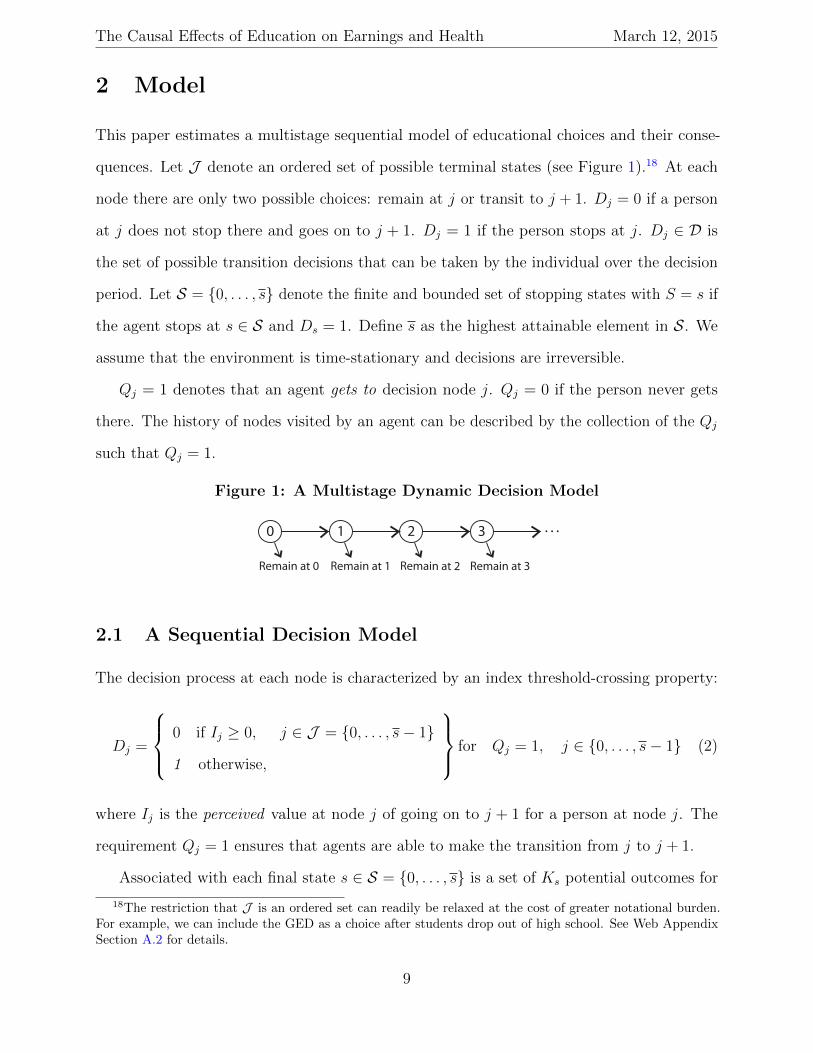
This paper estimates a multistage sequential model of educational choices and their conse-
quences. Let J denote an ordered set of possible terminal states (see Figure 1).18 At each
node there are only two possible choices: remain at j or transit to j + 1. Dj = 0 if a person
at j does not stop there and goes on to j + 1. Dj = 1 if the person stops at j. Dj ∈ D is
the set of possible transition decisions that can be taken by the individual over the decision
period. Let S = {0, . . . , s} denote the finite and bounded set of stopping states with S = s if
the agent stops at s ∈ S and Ds = 1. Define s as the highest attainable element in S. We
assume that the environment is time-stationary and decisions are irreversible.
Qj = 1 denotes that an agent gets to decision node j. Qj = 0 if the person never gets
there. The history of nodes visited by an agent can be described by the collection of the Qj
such that Qj = 1.
Figure 1: A Multistage Dynamic Decision Model
Remain at 2 Remain at 3Remain at 1 Remain at 0
0 1 2 3
2.1 A Sequential Decision Model
The decision process at each node is characterized by an index threshold-crossing property:
Dj =
0 if Ij ≥ 0, j ∈ J = {0, . . . , s− 1}
1 otherwise,
for Qj = 1, j ∈ {0, . . . , s− 1} (2)
where Ij is the perceived value at node j of going on to j + 1 for a person at node j. The
requirement Qj = 1 ensures that agents are able to make the transition from j to j + 1.
Associated with each final state s ∈ S = {0, . . . , s} is a set of Ks potential outcomes for
18The restriction that J is an ordered set can readily be relaxed at the cost of greater notational burden.For example, we can include the GED as a choice after students drop out of high school. See Web AppendixSection A.2 for details.
9
The Causal Effects of Education on Earnings and Health March 12, 2015
each agent with indices k ∈ Ks. We define Y ks as latent variables that map into potential
outcomes Y ks :
Y ks =
Y ks if Y k
s is continuous,
1 (Y ks ≥ 0) if Y k
s is a binary outcome,
k ∈ Ks, s ∈ S. (3)
Using the switching regression framework of Quandt (1958, 1972), the observed outcome Y k
for a k common across transitions is
Y k =∑s∈S
DsYks , k ∈ Ks. (4)
2.2 Parameterizations of the Decision Rules and Potential Out-
comes for Final States
Following a well-established tradition in the treatment effect and structural literatures, we
approximate Ij using a separable model:
Ij = φj (Z)︸︷︷︸Observedby analyst
− ηj︸︷︷︸Unobservedby analyst
, j ∈ {0, . . . , s− 1} (5)
where Z is a vector of variables observed by the analyst, components of which determine the
transition decisions of the agent at different stages and ηj is unobserved by the analyst. A
separable representation of the choice rule is an essential feature of LATE (Vytlacil, 2002)
and dynamic discrete choice models (Blevins, 2014).
Outcomes are also separable:
Y ks = τ ks (X)︸︷︷︸
Observedby analyst
+ Uks︸︷︷︸
Unobservedby analyst
, k ∈ Ks, s ∈ S, (6)
where X is a vector of observed determinants of outcomes and Uks is unobserved by the
10
The Causal Effects of Education on Earnings and Health March 12, 2015
analyst. Separability of the unobserved variables in the outcome equations is often invoked
in the structural literature but is not strictly required (see Blevins, 2014). It is not required
in the IV literature.
2.3 Structure of the Unobservables
Central to our main empirical strategy is the existence of a finite dimensional vector θ of
unobserved (by the economist) endowments that generate all of the dependence across the ηj
and the Uks . We assume that
ηj = −(θ′αj − νj, ) j ∈ {0, . . . , s− 1} (7)
and
Uks = θ′αks + ωks , k ∈ Ks, s ∈ S, (8)
where νj is an idiosyncratic error term for transition j.
Conditional on θ,X,Z, choices and outcomes are statistically independent. Thus con-
trolling for this set of variables eliminates selection effects. If the analyst knew θ, he/she
could use matching to identify the model.19
Standard “random effects” approaches in the structural literature integrate out θ and do
not interpret it. Our approach is different. We proxy θ using multiple measurements of it
and we identify, and correct for, errors in the proxy variables. The measurements facilitate
the interpretation of θ. We develop this intuition further in Section 4, after presenting the
rest of our model.
We array the νj, j ∈ J , into a vector ν = (ν0, ν1, . . . , νs−1) and the ηj into η =
(η0, . . . , ηs−1). ωks represents an idiosyncratic error term for outcome k in state s. Ar-
ray the ωks into a vector ωs = (ω1s , . . . , ω
Kss ). Array the Uk
s into vector Us = (U1s , . . . , U
Kss )
and array the Us into U = (U0, . . . ,Us).
19See Carneiro, Hansen, and Heckman (2003).
11
The Causal Effects of Education on Earnings and Health March 12, 2015
Letting “⊥⊥” denote statistical independence, we assume that
νj ⊥⊥ νl ∀ l 6= j l, j ∈ {0, . . . , s− 1} (A-1a)
ωks ⊥⊥ ωk′
s′ ∀ k 6= k′, s, s′ ∈ S (A-1bi)
ωks ⊥⊥ ωk′
s′ , ∀ k, k′, s 6= s′, s, s′ ∈ S (A-1bii)
ωs ⊥⊥ ν, ∀ s ∈ S (A-1c)
θ ⊥⊥ (X,Z) (A-1d)
(ωs,ν) ⊥⊥ (θ,X,Z) ∀ s ∈ S.20 (A-1e)
Assumption (A-1a) maintains independence of the shocks affecting schooling transitions;
assumption (A-1bi) and (A-1bii) maintain independence of shocks across outcomes within
states and across states; assumption (A-1c) maintains the independence of the shocks to
choice equations with the shocks to outcomes; assumption (A-1d) maintains independence of
θ with the observables; and assumption (A-1e) maintains independence of the shocks and θ
with the observed variables. Representations (7) and (8) and versions of assumptions (A-1d)
and (A-1e) play fundamental roles in the structural dynamic discrete choice literature.21
2.4 Measurement System for Unobserved Factors θ
We allow for the possibility that θ cannot be measured precisely, but that it can be proxied
with multiple measurements. We correct for the effects of measurement error in the proxy.
20Conditioning on X, we can weaken (A-1d) to
θ ⊥⊥ Z|X (A-1d′)
and (A-1e) to(ωs,ν) ⊥⊥ θ,Z|X (A-1e′)
All of the assumptions (A-1a)-(A-1e) can be reformulated to be conditional on X.21The Keane and Wolpin (1997) “types” can be interpreted as versions of θ that arise from the initial
conditions of their model. (7) and (8) capture the random effects specifications widely used in the discretechoice literature. (See Aguirregabiria, 2010 and Adda and Cooper, 2003.) Our model does not impose anyparticular information updating structure (e.g., iid shocks), the risk-neutrality of decision makers or theBellman equation decision structure widely used in the structural literature.
12
The Causal Effects of Education on Earnings and Health March 12, 2015
The structural literature treats the θ as nuisance variables, invokes conditional independence
assumptions, and integrates θ out using random effect procedures.22 Instead, we link θ to
measurements, and adjoin measurement equations to choice and outcome equations, rendering
θ interpretable.
Let T be a vector of M measurements on θ. They may consist of lagged or future values
of the outcome variables or additional measurements.23 The system of equations determining
T is:
T = Φ(X,θ, e), (9)
where X are observed variables, θ are the factors and
T =
T1
...
TM
=
Φ1(X,θ, e1)
...
ΦM(X,θ, eM)
where we array the ej into e = (e1, . . . , eM). We make the additional assumptions that:
ej ⊥⊥ el, j 6= l, j, l ∈ {1, . . . ,M} (A-1g)
and e ⊥⊥ (X,Z,θ,ν,ω). (A-1h)
For the purpose of identifying treatment effects, we do not need to identify each equation
of system (9). We just have to identify the span of θ that preserves the information on
θ in (9), and that is sufficient to produce conditional independence between choices and
outcomes.24 However, in this paper we estimate equation system (9).
22See e.g., Keane and Wolpin (1997); Rust (1994); Adda and Cooper (2003); Blevins (2014).23See, e.g., Abbring and Heckman (2007); Schennach, White, and Chalak (2012).24See e.g., Heckman, Schennach, and Williams (2013).
13
The Causal Effects of Education on Earnings and Health March 12, 2015
3 Defining Treatment Effects
A variety of ex post counterfactual outcomes and associated treatment effects can be generated
from our model. They can be used to predict the effects of manipulating education levels
through different policies for people of different backgrounds and abilities. They allow us to
understand the effectiveness of policies for different identifiable segments of the population,
and the benefits to people at different margins of choice.
In principle, we can define and estimate a variety of treatment effects, many of which are
implausible. For example, many empirical economists would not find estimates of the effect of
fixing (manipulating) Dj = 0 if Qj = 0 to be credible (i.e., the person for whom we fix Dj = 0
is not at the decision node to take the transition).25 In the spirit of credible econometrics, we
define treatment effects associated with fixing Dj = 0 conditioning on Qj = 1. This approach
blends structural and treatment effect approaches. Our causal parameters recognize agent
heterogeneity and are allowed to differ across populations, contrary to standard approaches
in structural econometrics.26
The person-specific treatment effect T kj for outcome k for an individual selected from the
population Qj = 1 with characteristics X = x,Z = z,θ = θ, making a decision at node j
between going on to j+ 1 or stopping at j is the difference between the individual’s outcomes
under the two actions. This can be written as
T kj [Y k|X = x,Z = z,θ = θ] : = (Y k|X = x,Z = z,θ = θ, F ix Dj = 0, Qj = 1)
− (Y k|X = x,Z = z,θ = θ, F ix Dj = 1, Qj = 1). (10)
The random variable (Y k|X = x,Z = z,θ = θ, F ix Dj = 0, Qj = 1) is the outcome variable
Y k at node j for a person with characteristics X = x,Z = z,θ = θ from the population
who attain node j (or higher), Qj = 1, and for whom we fix Dj = 0 so they go on to the next
25The distinction between fixing and conditioning traces back to Haavelmo (1943). White and Chalak(2009) use the terminology “setting” for the same notion. For a recent analysis of this crucial distinction, seeHeckman and Pinto (2015).
26See, e.g., Hansen and Sargent (1980).
14
The Causal Effects of Education on Earnings and Health March 12, 2015
node. Random variable (Y k|X = x,Z = z,θ = θ, F ix Dj = 1, Qj = 1) is defined for the
same individual but forces the person with these characteristics not to transit to the next
node.
We next present population level treatment effects based on (10). We focus our discussion
on means but we can also formulate distributional counterparts for all of the treatment effects
considered in this paper.
3.1 Dynamic Treatment Effects
A main contribution of this paper is to define and estimate treatment effects that take into
account the direct effect of moving to the next node of a decision tree, plus the benefits
associated with the further schooling that such movement opens up. This treatment effect is
the difference in expected outcomes arising from changing a single educational decision in a
sequential schooling model and tracing through its consequences, accounting for the dynamic
sequential nature of schooling.
The person-specific treatment effect can be decomposed into two components: the Direct
Effect of going from j to j + 1: DEkj = Y k
j+1 − Y kj , the effect often featured in the literature
on the returns to schooling, and the Continuation Value of going beyond j + 1:
Ckj+1 =
s−(j+1)∑r=1
[r∏l=1
(1−Dj+l)
](Y k
j+r+1 − Y kj+r).
27
Thus, at the individual level, the Total Effect of fixing Dj = 0 on Y k is decomposed into
T kj = DEkj + Ck
j+1. (11)
27The relationship between this notion of continuation value and the definition in the dynamic discretechoice literature is explored in Web Appendix A.3.
15
The Causal Effects of Education on Earnings and Health March 12, 2015
The associated population level average treatment effect conditional on Qj = 1 is
ATEkj :=
∫∫∫E[T kj (Y k|X = x,Z = z,θ = θ)] dFX,Z,θ(x, z,θ |Qj = 1) (12)
which can be decomposed into direct and continuation value components.
Because we do not specify or attempt to identify choice-node-specific agent information
sets, we can only identify ex-post treatment effects. Hence, we can identify continuation
values associated with choices, but cannot identify option values. However, a benefit of this
more agnostic approach is that it does not impose specific decision rules. Our model allows
for irrationality, regret, and mistakes in decision-making associated with agent maturation
and information acquisition.
3.2 Mean Differences Across Final Schooling Levels
Becker’s original approach (1964) can be interpreted to define returns to education as the
gains from choosing between a base and a terminal schooling level. Let Y ks′ be outcome k at
schooling level s′ and Y ks be outcome k at schooling level s. Conditioning on X = x and
θ = θ, the average treatment effect of s compared to s′ is E(Y ks − Y k
s′ |X = x,Z = z,θ = θ).
Integrating out X,Z,θ produces a pairwise ATE parameter over the available supports of
these variables.
A more empirically credible version, and the one we report here, calculates the mean gain
for the subset of the population that completes one of the two final schooling levels:
ATEks,s′ ≡
∫∫∫E(Y k
s − Y ks′ |X = x,Z = z,θ = θ) dFX,Z,θ(x, z,θ |Ds +Ds′ = 1). (13)
Conditioning in this fashion recognizes that the characteristics of people not making either
final choice could be far away from the population making one of those choices and hence
might be far away from having any empirical or policy relevance.28
28The estimated differences in treatment effects for the conditional and unconditional population are
16
The Causal Effects of Education on Earnings and Health March 12, 2015
3.3 Average Marginal Treatment Effects
In order to understand treatment effects for persons at the margin of indifference at each
node of the decision tree of Figure 1, we estimate the Average Marginal Treatment Effect
(AMTE).29 It is the average effect of transiting to the next node for individuals at the margin
of indifference between the two nodes:
AMTEkj := (14)∫∫∫E[T kj
(Y k|X = x,Z = z,θ = θ, |Ij | < ε
)]dFX,Z,θ(x, z, θ | Qj = 1, |Ij | ≤ ε),
where ε is an arbitrarily small neighborhood around the margin of indifference. These effects
are inclusive of all consequences of taking the transition at j, including the possibility of
attaining final schooling levels well beyond j. AMTE defines causal effects at well-defined
and empirically identified margins of choice. It is the proper measure of the marginal gross
benefit for evaluating the gains from moving from one stage of the decision tree to the next
for those at that margin of choice. In general it is distinct from LATE, which is not defined
for any specific margin of choice.30 Since we identify the distribution of Ij , we can identify the
characteristics of agents in the indifference set, something not possible using IV or matching.
The population distribution counterpart of AMTE is defined over the set of agents for
whom | Ij |≤ ε, which can be generated from our model: Pr(T kj < tkj |Qj = 1, |Ij| ≤ ε).
Distributional versions can be defined for all of the treatment effects considered in this section.
3.4 Policy Relevant Treatment Effects
The policy relevant treatment effect (PRTE) is the average treatment effect for those induced
to change their choices in response to a particular policy intervention. Let Y k(p) be the
aggregate outcome under policy p for outcome k. Let S(p) be the final state selected by
an agent under policy p. The policy relevant treatment effect from implementing policy p
not large for outcomes associated with the decision to enroll in college, but is substantial for the choice tograduate from college. See Tables A55, A57, A59, and A61 in the Web Appendix.
29See Carneiro, Heckman, and Vytlacil (2010, 2011).30See Heckman and Vytlacil (2007a) and Carneiro, Heckman, and Vytlacil (2010). The LATE can
correspond to people at multiple margins. See Angrist and Imbens (1995).
17
The Causal Effects of Education on Earnings and Health March 12, 2015
compared to policy p′ for outcome k is:
PRTEkp,p′ := (15)∫∫∫E(Y k(p)− Y k(p′)|X = x,Z = z,θ = θ, S(p) 6= S(p′))dFX,Z,θ(x, z,θ|S(p) 6= S(p′)),
where S(p) 6= S(p′) denotes the set of the characteristics of people for whom attained states
differ under the two policies. In general, it is different from AMTE because the agents affected
by a policy can be at multiple margins of choice. PRTE is often confused with LATE. In
general, they are different unless the proposed policy change coincides with the instrument
used to define LATE.31
4 Identification and Model Likelihood
The treatment effects defined in Section 3 can be identified using alternative empirical
approaches. The main approach used in this paper exploits the fact that conditional on
θ,X,Z, outcomes and choices are statistically independent. X and Z are observed. θ is
not. If θ were observed, one could condition on θ,X,Z and identify the model of Equations
(2) - (8) and the treatment effects that can be generated from it. We use nonlinear factor
model (9) to proxy θ.
Under the conditions presented in Web Appendix A.4, we can nonparametrically identify
the model of Equations (2) - (8) including the distribution of θ, as well as the Φ functions
and the distribution of e (which can be interpreted as measurement errors). Effectively, we
match on proxies for θ and correct for the effects of measurement error (e) in creating the
proxies. Such corrections are possible because with multiple measures on θ we can identify
the distribution of e.
Under full linearity assumptions, one can directly estimate the θ and use factor regression
31See Carneiro, Heckman, and Vytlacil (2011) for an empirical example. The differences between the twoparameters can be substantial as we show in Web Appendix A.5.2.
18
The Causal Effects of Education on Earnings and Health March 12, 2015
methods.32 Full details of this approach are spelled out in Web Appendix A.4.33 Another
approach to identification uses instrumental variables which, if available, under the conditions
presented in Web Appendix A.4 can be used to identify the structural model (2) - (8) without
factor structure (7) and (8).
The precise parameterization and the likelihood function for the model we estimate is
presented in Web Appendix A.6. While in principle it is possible to identify the model semi-
parametrically, in this paper we make parametric assumptions in order facilitate computation.
We subject the estimated model to rigorous goodness of fit tests which we pass.34
5 Our Data, A Benchmark OLS Analysis of the Out-
comes We Study and Our Exclusion Restrictions
We estimate our model on a sample of males extracted from the widely used National
Longitudinal Sample of Youth (NLSY 79).35 Before discussing estimates from our model, it
is informative to set the stage and present adjusted and unadjusted associations between
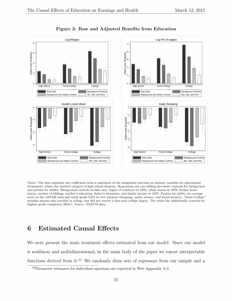
the outcomes we study and schooling. Figure 2 presents estimated regression relationships
between different levels of schooling (relative to high school dropouts) and the four outcomes
analyzed in this paper: wages, log present value of wages, health limitations, and smoking.36
The black bars in each panel show the unadjusted mean differences in outcomes for
persons at the indicated levels of educational attainment compared to those for high school
dropouts. Higher ability is associated with higher earnings and more schooling. However, as
shown by the grey bars in Figure 2, adjusting for family background and adolescent measures
of ability attenuates, but does not eliminate, the estimated effects of education.
32See, e.g., Heckman, Pinto, and Savelyev (2013) and the references cited therein.33As noted in Web Appendix A.4.1, and Heckman, Schennach, and Williams (2011), we do not need to
solve classical identification problems associated with estimating equation system (9) in order to extractmeasure-preserving transformations of θ on which we can condition in order to identify treatment effects. Inthe linear factor analysis literature these are rotation and normalization problems.
34See Web Appendix A.7.35Web Appendix A.8 presents a detailed discussion of the data we analyze and our exclusion restrictions.36Adjustments are made through linear regression.
19
The Causal Effects of Education on Earnings and Health March 12, 2015
Figure 2 shows that controlling for proxies for ability substantially reduces the observed
differences in earnings across educational groups. Nonetheless, there are still strong causal
effects of education. It has been claimed that a model that is linear in years of schooling fits
the data well.37 The white bar in Figure 2 displays the estimated adjusted effect of schooling
controlling for years of completed schooling as in Equation (1).38 The white bars in all figures
suggest that the linear-in-years-of-schooling Mincer specification (1) does not describe our
data. There are effects of schooling beyond those captured by a linear years of schooling
specification.
5.1 Exclusion Restrictions
As noted in Section 4, identification does not depend exclusively on conditional independence
assumptions associated with our factor model although they alone justify the identification
of our model using matching on mismeasured variables.39 Node-specific instruments can
nonparametrically identify treatment effects without invoking the full set of conditional
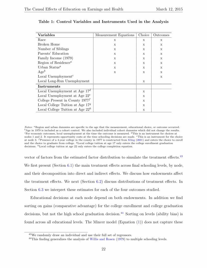
independence assumptions.40 We have a variety of exclusion restrictions that affect choices
but not outcomes. Table 1 documents the X and Z used in this paper. Our instruments are
traditional in the literature that estimates the causal effects of education.41
37See e.g., Card (1999, 2001). Heckman, Lochner, and Todd (2006) dispute this claim.38Mis-measurement of schooling is less of a concern in our data as the survey asks numerous educational
questions every year which we use to determine an individual’s final schooling state.39See Carneiro, Hansen, and Heckman (2003).40See Web Appendix A.4.41For example, presence of a nearby college or distance to college is used by Card (2012); Cameron and
Taber (2004); Kling (2001); Carneiro, Meghir, and Parey (2013); Cawley, Conneely, Heckman, and Vytlacil(1997); Heckman, Carneiro, and Vytlacil (2011); and Eisenhauer, Heckman, and Vytlacil (2015). Local tuitionat two or four year colleges is used as an instrument by Kane and Rouse (1993); Heckman, Carneiro, andVytlacil (2011); Eisenhauer, Heckman, and Vytlacil (2015); and Cameron and Taber (2004). Local labormarket shocks are used by Heckman, Carneiro, and Vytlacil (2011) and Eisenhauer, Heckman, and Vytlacil(2015).
20
The Causal Effects of Education on Earnings and Health March 12, 2015
Figure 2: Raw and Adjusted Benefits from Education0
.2.4
.6.8
Gai
ns o
ver
Dro
pout
s
High School Some College College
Raw Data Background Controls
Background and Ability Controls BG, Abil, and HGC
Log Wages
0.2
.4.6
.81
Gai
ns o
ver
Dro
pout
s
High School Some College College
Raw Data Background Controls
Background and Ability Controls BG, Abil, and HGC
Log PV of wages
−.3
−.2
−.1
0G
ains
ove
r D
ropo
uts
High School Some College College
Raw Data Background Controls
Background and Ability Controls BG, Abil, and HGC
Health Limits Work
−.6
−.5
−.4
−.3
−.2
−.1
Gai
ns o
ver
Dro
pout
s
High School Some College College
Raw Data Background Controls
Background and Ability Controls BG, Abil, and HGC
Daily Smoking
Notes: The bars represent the coefficients from a regression of the designated outcome on dummy variables for educationalattainment, where the omitted category is high school dropout. Regressions are run adding successive controls for backgroundand proxies for ability. Background controls include race, region of residence in 1979, urban status in 1979, broken homestatus, number of siblings, mother’s education, father’s education, and family income in 1979. Proxies for ability are averagescore on the ASVAB tests and ninth grade GPA in core subjects (language, math, science, and social science). “Some College”includes anyone who enrolled in college, but did not receive a four-year college degree. The white bar additionally controls forhighest grade completed (HGC). Source: NLSY79 data.
6 Estimated Causal Effects
We next present the main treatment effects estimated from our model. Since our model
is nonlinear and multidimensional, in the main body of the paper we report interpretable
functions derived from it.42 We randomly draw sets of regressors from our sample and a
42Parameter estimates for individual equations are reported in Web Appendix A.9.
21
The Causal Effects of Education on Earnings and Health March 12, 2015
Table 1: Control Variables and Instruments Used in the Analysis
Variables Measurement Equations Choice Outcomes
Race x x xBroken Home x x xNumber of Siblings x x xParents’ Education x x xFamily Income (1979) x x xRegion of Residencea x x xUrban Statusa x x xAgeb x x xLocal Unemploymentc xLocal Long-Run Unemployment x
Instruments
Local Unemployment at Age 17d xLocal Unemployment at Age 22e xCollege Present in County 1977f xLocal College Tuition at Age 17g xLocal College Tuition at Age 22h x
Notes: aRegion and urban dummies are specific to the age that the measurement, educational choice, or outcome occurred.bAge in 1979 is included as a cohort control. We also included individual cohort dummies which did not change the results.cFor economic outcomes, local unemployment at the time the outcome is measured. dThis is an instrument for choices atnodes 1 and 2. It represents opportunity costs at the time schooling decisions are made. eThis is an instrument for the choiceat node 3. fPresence of a 4-year college in the county in 1977 is constructed from Kling (2001) and enters the choice to enrolland the choice to graduate from college. gLocal college tuition at age 17 only enters the college enrollment graduationdecisions. hLocal college tuition at age 22 only enters the college completion equation.
vector of factors from the estimated factor distribution to simulate the treatment effects.43
We first present (Section 6.1) the main treatment effects across final schooling levels, by node,
and their decomposition into direct and indirect effects. We discuss how endowments affect
the treatment effects. We next (Section 6.2) discuss distributions of treatment effects. In
Section 6.3 we interpret these estimates for each of the four outcomes studied.
Educational decisions at each node depend on both endowments. In addition we find
sorting on gains (comparative advantage) for the college enrollment and college graduation
decisions, but not the high school graduation decision.44 Sorting on levels (ability bias) is
found across all educational levels. The Mincer model (Equation (1)) does not capture these
43We randomly draw an individual and use their full set of regressors.44This finding generalizes the analysis of Willis and Rosen (1979) to multiple schooling levels.
22
The Causal Effects of Education on Earnings and Health March 12, 2015
types of sorting patterns. It overlooks the differences in the distributions of returns across
schooling levels.
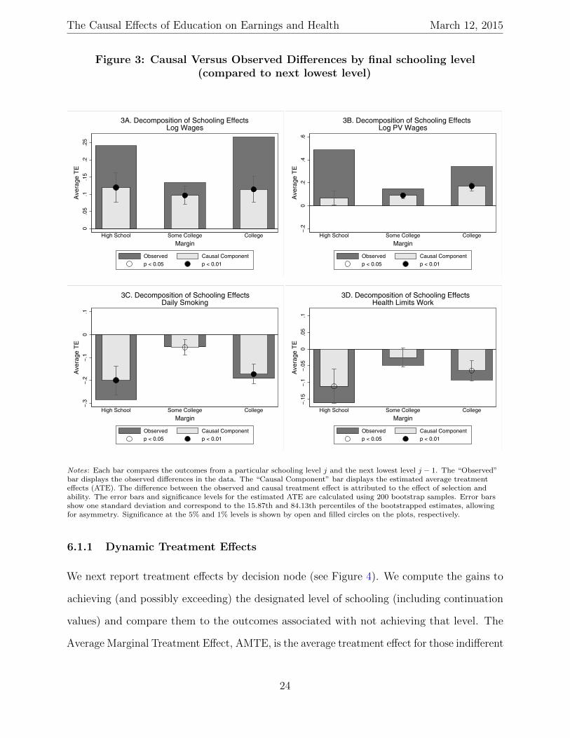
6.1 The Estimated Causal Effects of Educational Choices
We first compare the outcomes from final schooling level s with those from s − 1.45 The
estimated treatment effects of education on log wages, log PV wage income, smoking, and
health limits work are shown in Figure 3.46 For each outcome, the bars labeled “Observed”
display the unadjusted raw differences in the data. The bars labeled “Causal Component”
display the average treatment effect obtained from comparing the outcomes associated with
a particular schooling level s relative to s− 1. These are defined for individuals at s or s− 1.
There are substantial causal effects on earnings and health at each level of schooling. But at
most levels there is also considerable ability bias.
45See expression (13) for the case s′ = s− 1.46These are calculated by simulating the mean outcomes for the designated state and comparing it with
the mean-simulated outcome for the state directly below it for the subpopulation of persons who are in eitherof the states.
23
The Causal Effects of Education on Earnings and Health March 12, 2015
Figure 3: Causal Versus Observed Differences by final schooling level(compared to next lowest level)
0.0
5.1
.15
.2.2
5A
vera
ge T
E
High School Some College CollegeMargin
Observed Causal Componentp < 0.05 p < 0.01
3A. Decomposition of Schooling EffectsLog Wages
−.2
0.2
.4.6
Ave
rage
TE
High School Some College CollegeMargin
Observed Causal Componentp < 0.05 p < 0.01
3B. Decomposition of Schooling EffectsLog PV Wages
−.3
−.2
−.1
0.1
Ave
rage
TE
High School Some College CollegeMargin
Observed Causal Componentp < 0.05 p < 0.01
3C. Decomposition of Schooling EffectsDaily Smoking
−.15
−.1
−.05
0.0
5.1
Ave
rage
TE
High School Some College CollegeMargin
Observed Causal Componentp < 0.05 p < 0.01
3D. Decomposition of Schooling EffectsHealth Limits Work
Notes: Each bar compares the outcomes from a particular schooling level j and the next lowest level j − 1. The “Observed”bar displays the observed differences in the data. The “Causal Component” bar displays the estimated average treatmenteffects (ATE). The difference between the observed and causal treatment effect is attributed to the effect of selection andability. The error bars and significance levels for the estimated ATE are calculated using 200 bootstrap samples. Error barsshow one standard deviation and correspond to the 15.87th and 84.13th percentiles of the bootstrapped estimates, allowingfor asymmetry. Significance at the 5% and 1% levels is shown by open and filled circles on the plots, respectively.
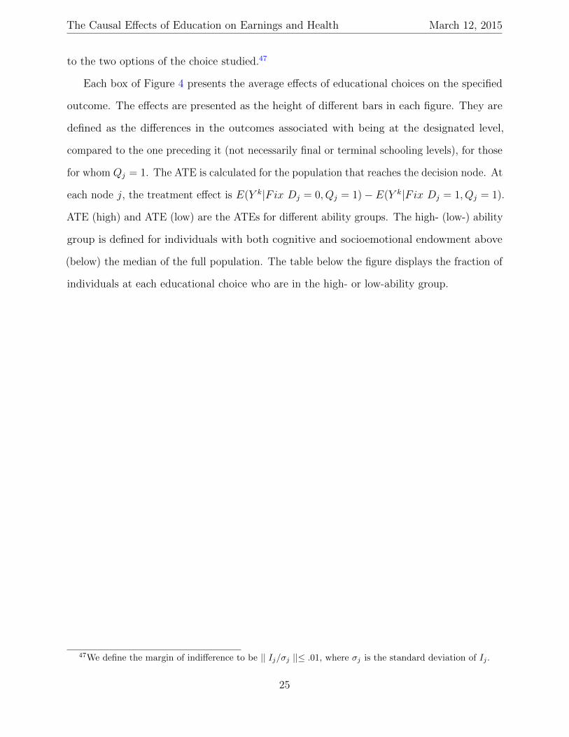
6.1.1 Dynamic Treatment Effects
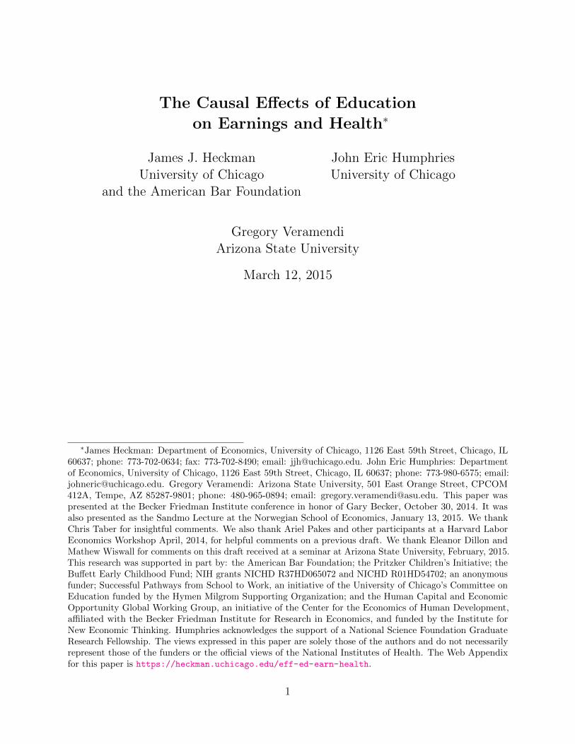
We next report treatment effects by decision node (see Figure 4). We compute the gains to
achieving (and possibly exceeding) the designated level of schooling (including continuation
values) and compare them to the outcomes associated with not achieving that level. The
Average Marginal Treatment Effect, AMTE, is the average treatment effect for those indifferent
24
The Causal Effects of Education on Earnings and Health March 12, 2015
to the two options of the choice studied.47
Each box of Figure 4 presents the average effects of educational choices on the specified
outcome. The effects are presented as the height of different bars in each figure. They are
defined as the differences in the outcomes associated with being at the designated level,
compared to the one preceding it (not necessarily final or terminal schooling levels), for those
for whom Qj = 1. The ATE is calculated for the population that reaches the decision node. At
each node j, the treatment effect is E(Y k|Fix Dj = 0, Qj = 1)− E(Y k|Fix Dj = 1, Qj = 1).
ATE (high) and ATE (low) are the ATEs for different ability groups. The high- (low-) ability
group is defined for individuals with both cognitive and socioemotional endowment above
(below) the median of the full population. The table below the figure displays the fraction of
individuals at each educational choice who are in the high- or low-ability group.
47We define the margin of indifference to be || Ij/σj ||≤ .01, where σj is the standard deviation of Ij .
25
The Causal Effects of Education on Earnings and Health March 12, 2015
Figure 4: Treatment Effects of Outcomes by Decision NodeE(Y k|Fix Dj = 0, Qj = 1)− E(Y k|Fix Dj = 1, Qj = 1)
−.1
0.1
.2.3
Ave
rage
TE
Graduate HS Enroll in Coll. Graduate Coll.Decision Node
AMTE ATE ATE (low)ATE (high) p < 0.05 p < 0.01
4A. Treatment Effects: Log Wages
−.2
−.1
0.1
.2.3
Ave
rage
TE
Graduate HS Enroll in Coll. Graduate Coll.Decision Node
AMTE ATE ATE (low)ATE (high) p < 0.05 p < 0.01
4B. Treatment Effects: Log PV Wages
−.4
−.2
0.2
Ave
rage
TE
Graduate HS Enroll in Coll. Graduate Coll.Decision Node
AMTE ATE ATE (low)ATE (high) p < 0.05 p < 0.01
4C. Treatment Effects: Daily Smoking−.
2−.
10
.1.2
Ave
rage
TE
Graduate HS Enroll in Coll. Graduate Coll.Decision Node
AMTE ATE ATE (low)ATE (high) p < 0.05 p < 0.01
4D. Treatment Effects: Health Limits Work
Sorting on Ability
Low Ability High AbilityD1: Dropping from HS vs. Graduating from HS 0.31 0.31D2: HS Graduate vs. College Enrollment 0.22 0.38D3: Some College vs. 4-year college degree 0.13 0.51
Notes: Each schooling level might provide the option to pursuing higher schooling levels. Only final schooling levels do notprovide an option value. The error bars and significance levels for the estimated ATE are calculated using 200 bootstrapsamples. Error bars show one standard deviation and correspond to the 15.87th and 84.13th percentiles of the bootstrappedestimates, allowing for asymmetry. Significance at the 5% and 1% level are shown by hollow and black circles on the plotsrespectively. The figure reports various treatment effects for those who reach the decision node, including the estimated ATEconditional on endowment levels. The high- (low-) ability group is defined as those individuals with cognitive andsocioemotional endowments above (below) the median in the overall population. The table below the figure shows theproportion of individuals at each decision (Qj = 1) that are high and low ability. The larger proportion of the individuals arehigh ability and a smaller proportion are low ability in later educational decisions. In this table, final schooling levels arehighlighted using bold letters.
26
The Causal Effects of Education on Earnings and Health March 12, 2015
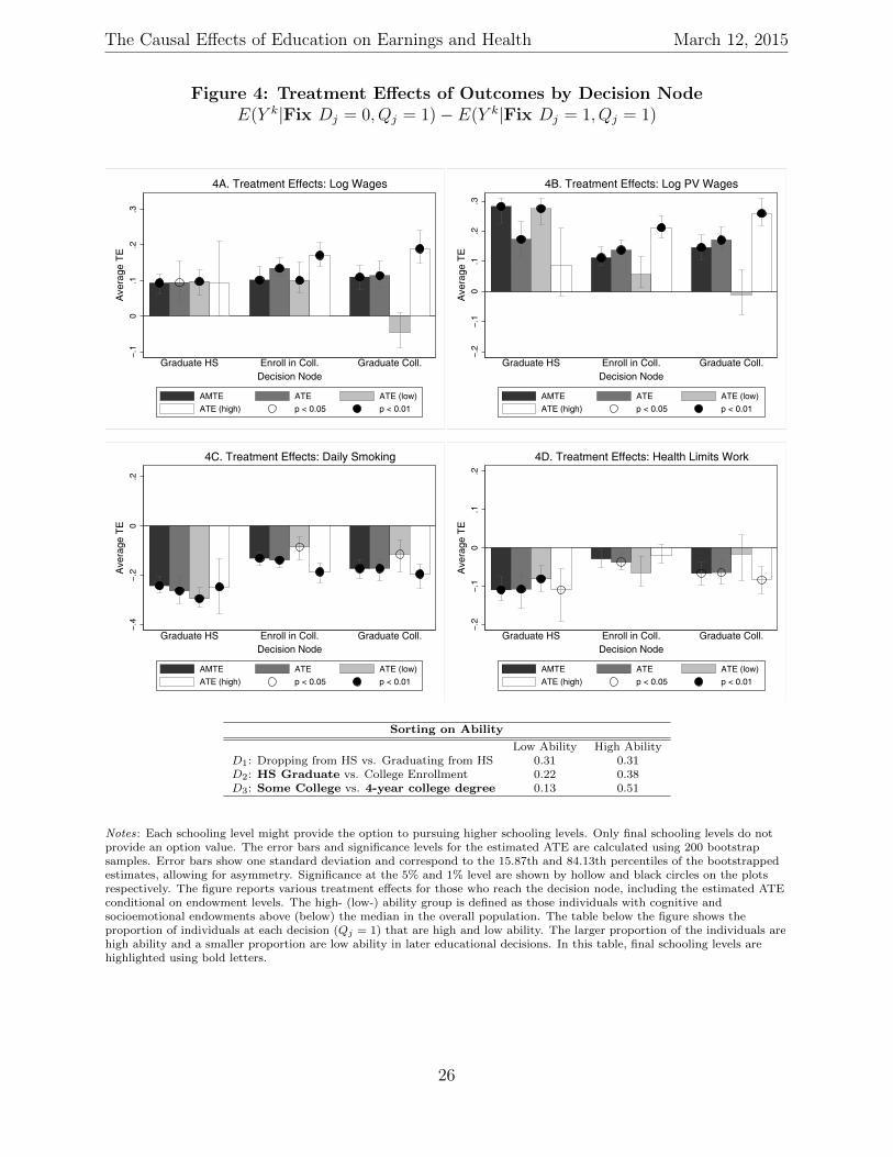
6.1.2 Continuation Values
We next decompose the node-specific treatment effects reported in Table 4 into the total
effect and the continuation value components. Figure 5 presents graphs of each causal effect
in Figure 4 and shows the continuation value component (in white). Continuation values are
important components of the dynamic treatment effects for all outcomes except health limits
work.
Figure 5: Dynamic Treatment Effects:Continuation Values and Total Treatment Effects by Node
0.0
5.1
.15
.2A
vera
ge T
E
Graduate HS Enroll in CollegeDecision Node
AMTE ATE ATE (low) ATE (high)Cont. Value p < 0.05 p < 0.01 p < 0.05 for CV=0
5A. Total Effect and Continuation Value:Log Wages
0.1
.2.3
Ave
rage
TE
Graduate HS Enroll in CollegeDecision Node
AMTE ATE ATE (low) ATE (high)Cont. Value p < 0.05 p < 0.01 p < 0.05 for CV=0
5B. Total Effect and Continuation Value:Log PV Wages
−.4
−.3
−.2
−.1
0A
vera
ge T
E
Graduate HS Enroll in CollegeDecision Node
AMTE ATE ATE (low) ATE (high)Cont. Value p < 0.05 p < 0.01 p < 0.05 for CV=0
5C. Total Effect and Continuation Value:Daily Smoking
−.2
−.15
−.1
−.05
0A
vera
ge T
E
Graduate HS Enroll in CollegeDecision Node
AMTE ATE ATE (low) ATE (high)Cont. Value p < 0.05 p < 0.01 p < 0.05 for CV=0
5D. Total Effect and Continuation Value:Health Limits Work
Notes: High-ability individuals are those in the top 50% of the distributions of both cognitive and socioemotionalendowments. Low-ability individuals are those in the bottom 50% of the distributions of both cognitive and socioemotionalendowments. The error bars and significance levels for the estimated ATE are calculated using 200 bootstrap samples. Errorbars show one standard deviation and correspond to the 15.87th and 84.13th percentiles of the bootstrapped estimates,allowing for asymmetry. Significance at the 5% and 1% level are shown by hollow and black circles on the plots respectively.Statistical significance for continuation values at the 5% level are shown by x. Section 3 provides details on how thecontinuation values and treatment effects are calculated.
27
The Causal Effects of Education on Earnings and Health March 12, 2015
6.1.3 The Effects on Cognitive and Noncognitive Endowments on Treatment
Effects
While we disaggregate the treatment effects for “high” and “low” endowment individuals in
Figure 4, this division is coarse. A byproduct of our approach is that we can determine the
contribution of cognitive and noncognitive endowments (θ) to explaining estimated treatment
effects. We can decompose the overall effects of θ into their contribution to the causal effects
at each node and the contribution of endowments to attaining that node. We find substantial
contributions of θ to each component at each node.
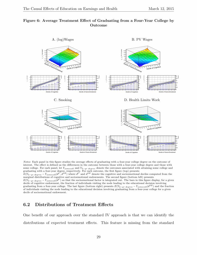
To illustrate, the panels in Figure 6 display the estimated average treatment effect of
getting a four-year degree (compared to stopping with some college) for each decile pair of
cognitive and noncognitive endowments.48,49 Treatment effects in general depend on both
measures of ability. Moreover, different outcomes depend in different ways on the two
dimensions of ability. For example, the treatment effect of graduating college is increasing in
both dimensions for present value of wages, but the reductions in health limitations with
education depend mostly on cognitive endowments.
48Web Appendix A.10 reports a full set of results.49They show average benefits by decile over the full population, rather than for the population that reaches
each node.
28
The Causal Effects of Education on Earnings and Health March 12, 2015
Figure 6: Average Treatment Effect of Graduating from a Four-Year College byOutcome
A. (log)Wages B. PV Wages
Decile of Cognitive1 2 3 4 5 6 7 8 9 10
Decile of Socio-Emotional
12345678910
Log
-wag
es0
- y
1y
-0.2
-0.1
0
0.1
0.2
0.3
Decile of Cognitive1 2 3 4 5 6 7 8 9 10
Log
-wag
es0
- y
1y
-0.2
-0.1
0
0.1
0.2
0.3
Fra
ctio
n
0
0.05
0.1
0.15
0.2
0.25
0.3
0.35
Decile of Socio-Emotional1 2 3 4 5 6 7 8 9 10
Log
-wag
es0
- y
1y
-0.2
-0.1
0
0.1
0.2
0.3
Fra
ctio
n
0
0.05
0.1
0.15
0.2
0.25
0.3
Decile of Cognitive1 2 3 4 5 6 7 8 9 10
Decile of Socio-Emotional
12345678910
PV
of I
ncom
e0
- y
1y -0.1
0
0.1
0.2
0.3
0.4
Decile of Cognitive1 2 3 4 5 6 7 8 9 10
PV
of I
ncom
e0
- y
1y
-0.1
0
0.1
0.2
0.3
0.4
Fra
ctio
n
0
0.05
0.1
0.15
0.2
0.25
0.3
0.35
Decile of Socio-Emotional1 2 3 4 5 6 7 8 9 10
PV
of I
ncom
e0
- y
1y
-0.1
0
0.1
0.2
0.3
0.4
Fra
ctio
n
0
0.05
0.1
0.15
0.2
0.25
0.3
C. Smoking D. Health Limits Work
Decile of Cognitive1 2 3 4 5 6 7 8 9 10
Decile of Socio-Emotional
12345678910
Sm
oker
0 -
y1y
-0.3
-0.2
-0.1
0
0.1
Decile of Cognitive1 2 3 4 5 6 7 8 9 10
Sm
oker
0 -
y1
y
-0.3
-0.2
-0.1
0
0.1
Fra
ctio
n
0
0.05
0.1
0.15
0.2
0.25
0.3
0.35
Decile of Socio-Emotional1 2 3 4 5 6 7 8 9 10
Sm
oker
0 -
y1
y
-0.3
-0.2
-0.1
0
0.1
Fra
ctio
n
0
0.05
0.1
0.15
0.2
0.25
0.3
Decile of Cognitive1 2 3 4 5 6 7 8 9 10
Decile of Socio-Emotional
12345678910 W
ork
Lim
ited
by H
ealth
0 -
y1y
-0.25-0.2
-0.15-0.1
-0.050
0.050.1
0.150.2
Decile of Cognitive
1 2 3 4 5 6 7 8 9 10
Wor
k Li
mite
d by
Hea
lth0
- y
1y
-0.25
-0.2
-0.15
-0.1
-0.05
0
0.05
0.1
0.15
0.2
Fra
ctio
n
0
0.05
0.1
0.15
0.2
0.25
0.3
0.35
Decile of Socio-Emotional1 2 3 4 5 6 7 8 9 10
Wor
k Li
mite
d by
Hea
lth0
- y
1y
-0.25
-0.2
-0.15
-0.1
-0.05
0
0.05
0.1
0.15
0.2
Fra
ctio
n
0
0.05
0.1
0.15
0.2
0.25
0.3
Notes: Each panel in this figure studies the average effects of graduating with a four-year college degree on the outcome ofinterest. The effect is defined as the differences in the outcome between those with a four-year college degree and those withsome college. For each panel, let Ysomecoll and Y4−yr degree denote the outcomes associated with attaining some college andgraduating with a four-year degree, respectively. For each outcome, the first figure (top) presentsE(Y4−yr degree − Ysomecoll|dC , dSE) where dC and dSE denote the cognitive and socioemotional deciles computed from themarginal distributions of cognitive and socioemotional endowments. The second figure (bottom left) presentsE(Y4−yr degree − Ysomecoll|dC) so that the socioemotional factor is integrated out. The bars in this figure display, for a givendecile of cognitive endowment, the fraction of individuals visiting the node leading to the educational decision involvinggraduating from a four-year college. The last figure (bottom right) presents E(Y4−yr degree − Ysomecoll|dSE) and the fractionof individuals visiting the node leading to the educational decision involving graduating from a four-year college for a givendecile of socioemotional endowment.
6.2 Distributions of Treatment Effects
One benefit of our approach over the standard IV approach is that we can identify the
distributions of expected treatment effects. This feature is missing from the standard
29
The Causal Effects of Education on Earnings and Health March 12, 2015
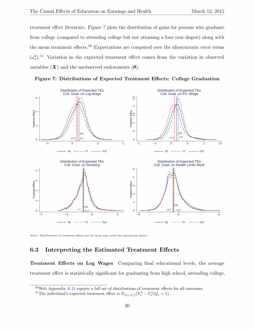
treatment effect literature. Figure 7 plots the distribution of gains for persons who graduate
from college (compared to attending college but not attaining a four-year degree) along with
the mean treatment effects.50 Expectations are computed over the idiosyncratic error terms
(ωks ).51 Variation in the expected treatment effect comes from the variation in observed
variables (X) and the unobserved endowments (θ).
Figure 7: Distributions of Expected Treatment Effects: College Graduation
ATE
ATTATUT01
23
Tre
atm
en E
ffect
−.5 0 .5 1
TE TT TUT
Distribution of Expected TEsColl. Grad. on Log Wage
ATE
ATTATUT
0.5
11.
52
2.5
Tre
atm
en E
ffect
−1 −.5 0 .5 1 1.5
TE TT TUT
Distribution of Expected TEsColl. Grad. on PV−Wage
ATE
ATUT01
23
4T
reat
men
Effe
ct
−1 −.5 0 .5
TE TT TUT
Distribution of Expected TEsColl. Grad. on Smoking
ATT
ATE
ATUT01
23
45
Tre
atm
en E
ffect
−.5 0 .5
TE TT TUT
Distribution of Expected TEsColl. Grad. on Health Limits Work
ATT
Notes: Distributions of treatment effects are for those who reach the educational choice.
6.3 Interpreting the Estimated Treatment Effects
Treatment Effects on Log Wages Comparing final educational levels, the average
treatment effect is statistically significant for graduating from high school, attending college,
50Web Appendix A.11 reports a full set of distributions of treatment effects for all outcomes.51The individual’s expected treatment effect is E{ωs,ω′s}(Y
ks − Y k
s′ |Qs = 1).
30
The Causal Effects of Education on Earnings and Health March 12, 2015
and attaining a four-year college degree. About half of the observed difference in wages at
age 30 is explained by the X,Z, and θ.
Estimates for node-specific treatment effects show that more schooling causally boosts
wages although low-endowment individuals gain very little from getting a four-year college
degree. Figure 4 shows that individuals with high cognitive ability capture most of the
gains from a four-year degree. In fact, our estimates suggest those with very low cognitive
and socioemotional endowments lose wage income at age 30 by graduating from college.52
Figure 5 shows that continuation values are an important component of average treatment
effects for high ability individuals. Figure 6 shows that most of the effect of abilities on the
average treatment effect of college graduation comes from cognitive channels. Figure 7 shows
the sorting pattern for college graduation. Even though it is not imposed by our estimation
procedure, we find sorting on gains.
Treatment Effects on Present Value of Wage Income The pattern for the present
value of wages is similar to that for wages with some interesting exceptions. Figures 4 and 5
show that low ability students appear to benefit substantially from graduating from high
school, while only high ability individuals benefit from enrolling in and graduating from
college. The treatment effect of college graduation is especially strong for high ability students.
The benefits to low ability people and people at the margin of graduating high school come
primarily from direct effects. The larger effects for present values than for wages comes from
labor supply responses of high school graduates.53 We find sorting on gains for the higher
educational nodes. Figure 6 shows that noncognitive endowments play a much stronger role
in generating the average treatment effect of college graduation on the PV of wages than
they do for wages.
52See Web Appendix Section A.1.2 for a brief overview of the literature on the outcomes considered inthis paper.
53See Heckman, Humphries, and Kautz (2014, Chapter 5).
31
The Causal Effects of Education on Earnings and Health March 12, 2015
Treatment Effects on Smoking Controlling for unobserved endowments, education
causally reduces smoking. The endowments and observables account for about one-third of
the observed effect of education. The effects are especially strong for high school graduation.
Looking at the node-specific treatment effects, each level of education has a substantial causal
effect in reducing smoking. For high-endowment individuals, more than half of the average
treatment effect of graduating high school and enrolling in college is derived from continuation
values. Almost all of the treatment effect comes from the direct effect for low-endowment
individuals.
Treatment Effects on Health Limits Work There are strong treatment effects for
graduating high school but much weaker, and less precisely determined, treatment effects
at higher levels of education. Continuation values are small and generally statistically
insignificant. As in the case of smoking, the treatment effects are especially strong for high
ability individuals except in this case noncognitive endowments play a small role.
6.4 Heterogeneity in Returns Across Schooling Levels
Mincer equation (1) is often invoked in the empirical literature.54 Its linear specification
avoids the need for stage-specific instruments. It implies that the return to an additional
year of schooling is the same across schooling levels (although it may differ across persons).
Returns across different schooling levels are summarized by a single number, ρi.
Most of the literature estimates linear-in-years-of-schooling models using OLS. Figure 2
shows that adding dummy variables to a linear-in-schooling specification substantially im-
proves the fit of the model.55 We have already noted that sorting by gains differs by
educational level. Using this methodology, linearity in years of schooling for wage equations
is decisively rejected in many data sets and it is rejected in our data.56
54See, e.g., the surveys in Card (1999, 2001) and Heckman, Lochner, and Todd (2006).55Card’s (1999, 2001) claims about linearity are based on OLS, as are most claims in the literature.
(Heckman, Lochner, and Todd (2006)). We formally test this proposition in Web Appendix A.12.56See the evidence discussed in Heckman, Lochner, and Todd (2006) and in Web Appendix A.12.
32
The Causal Effects of Education on Earnings and Health March 12, 2015
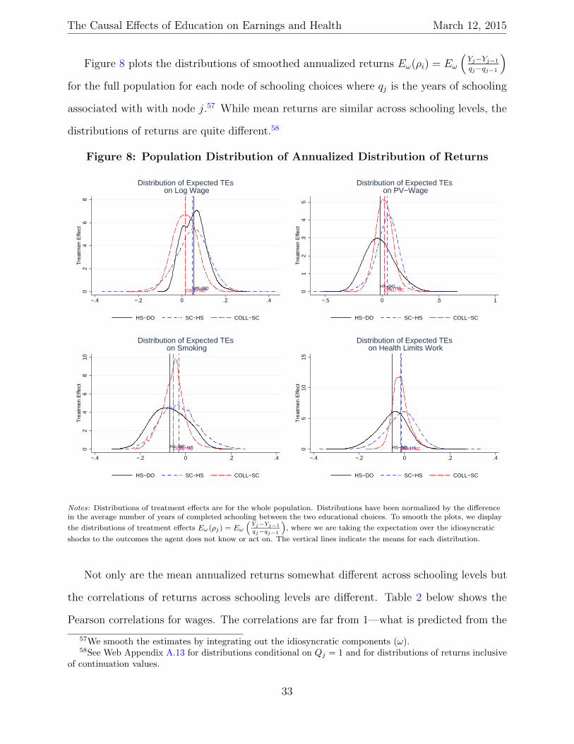
Figure 8 plots the distributions of smoothed annualized returns Eω(ρi) = Eω
(Yj−Yj−1
qj−qj−1
)for the full population for each node of schooling choices where qj is the years of schooling
associated with with node j.57 While mean returns are similar across schooling levels, the
distributions of returns are quite different.58
Figure 8: Population Distribution of Annualized Distribution of Returns
HS−DOSC−HSCOLL−SC02
46
8T
reat
men
Effe
ct
−.4 −.2 0 .2 .4
HS−DO SC−HS COLL−SC
Distribution of Expected TEs on Log Wage
HS−DOSC−HSCOLL−SC01
23
45
Tre
atm
en E
ffect
−.5 0 .5 1
HS−DO SC−HS COLL−SC
Distribution of Expected TEs on PV−Wage
HS−DOSC−HSCOLL−SC02
46
810
Tre
atm
en E
ffect
−.4 −.2 0 .2 .4
HS−DO SC−HS COLL−SC
Distribution of Expected TEs on Smoking
HS−DOSC−HSCOLL−SC05
1015
Tre
atm
en E
ffect
−.4 −.2 0 .2 .4
HS−DO SC−HS COLL−SC
Distribution of Expected TEs on Health Limits Work
Notes: Distributions of treatment effects are for the whole population. Distributions have been normalized by the differencein the average number of years of completed schooling between the two educational choices. To smooth the plots, we display
the distributions of treatment effects Eω(ρj) = Eω
(Yj−Yj−1
qj−qj−1
), where we are taking the expectation over the idiosyncratic
shocks to the outcomes the agent does not know or act on. The vertical lines indicate the means for each distribution.
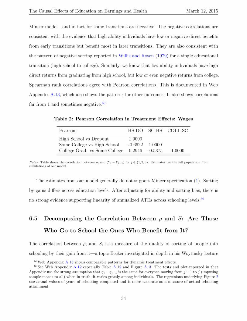
Not only are the mean annualized returns somewhat different across schooling levels but
the correlations of returns across schooling levels are different. Table 2 below shows the
Pearson correlations for wages. The correlations are far from 1—what is predicted from the
57We smooth the estimates by integrating out the idiosyncratic components (ω).58See Web Appendix A.13 for distributions conditional on Qj = 1 and for distributions of returns inclusive
of continuation values.
33
The Causal Effects of Education on Earnings and Health March 12, 2015
Mincer model—and in fact for some transitions are negative. The negative correlations are
consistent with the evidence that high ability individuals have low or negative direct benefits
from early transitions but benefit most in later transitions. They are also consistent with
the pattern of negative sorting reported in Willis and Rosen (1979) for a single educational
transition (high school to college). Similarly, we know that low ability individuals have high
direct returns from graduating from high school, but low or even negative returns from college.
Spearman rank correlations agree with Pearson correlations. This is documented in Web
Appendix A.13, which also shows the patterns for other outcomes. It also shows correlations
far from 1 and sometimes negative.59
Table 2: Pearson Correlation in Treatment Effects: Wages
Pearson: HS-DO SC-HS COLL-SC
High School vs Dropout 1.0000Some College vs High School -0.6622 1.0000College Grad. vs Some College 0.2946 -0.5375 1.0000
Notes: Table shows the correlation between ρi and (Yj − Yj−1) for j ∈ {1, 2, 3}. Estimates use the full population fromsimulations of our model.
The estimates from our model generally do not support Mincer specification (1). Sorting
by gains differs across education levels. After adjusting for ability and sorting bias, there is
no strong evidence supporting linearity of annualized ATEs across schooling levels.60
6.5 Decomposing the Correlation Between ρ and S: Are Those
Who Go to School the Ones Who Benefit from It?
The correlation between ρi and Si is a measure of the quality of sorting of people into
schooling by their gain from it—a topic Becker investigated in depth in his Woytinsky lecture
59Web Appendix A.13 shows comparable patterns for dynamic treatment effects.60See Web Appendix A.12 especially Table A.12 and Figure A13. The tests and plot reported in that
Appendix use the strong assumption that qj − qj−1 is the same for everyone moving from j− 1 to j (imputingsample means to all) when in truth, it varies greatly among individuals. The regressions underlying Figure 2use actual values of years of schooling completed and is more accurate as a measure of actual schoolingattainment.
34
The Causal Effects of Education on Earnings and Health March 12, 2015
(1967,1991). We have already established that the distributions of returns differ across
schooling levels and the returns across schooling levels are far from perfectly correlated.
It is thus of interest to push our analysis a bit further and investigate the correlation of
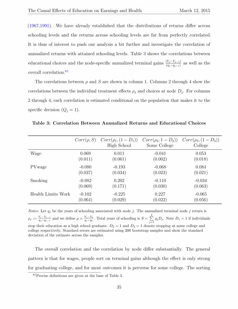
annualized returns with attained schooling levels. Table 3 shows the correlations between
educational choices and the node-specific annualized terminal gains(Yj−Yj−1)
(qj−qj−1)as well as the
overall correlation.61
The correlations between ρ and S are shown in column 1. Columns 2 through 4 show the
correlations between the individual treatment effects ρj and choices at node Dj . For columns
2 through 4, each correlation is estimated conditional on the population that makes it to the
specific decision (Qj = 1).
Table 3: Correlation Between Annualized Returns and Educational Choices
Corr(ρ, S) Corr(ρ1, (1−D1)) Corr(ρ2, 1−D2)) Corr(ρ3, (1−D3))High School Some College College
Wage 0.069 0.011 -0.041 0.053(0.011) (0.061) (0.002) (0.018)
PVwage -0.080 -0.193 -0.068 0.084(0.037) (0.034) (0.023) (0.021)
Smoking -0.082 0.202 -0.110 -0.034(0.069) (0.171) (0.030) (0.063)
Health Limits Work -0.102 -0.225 0.227 -0.065(0.064) (0.029) (0.022) (0.056)
Notes: Let qj be the years of schooling associated with node j. The annualized terminal node j return is
ρj :=Yj−Yj−1
qj−qj−1and we define ρ =
Yj−Y0
qj−q0 . Total years of schooling is S =s∑
j=1
qjDj . Note D1 = 1 if individuals
stop their education as a high school graduate. D2 = 1 and D3 = 1 denote stopping at some college andcollege respectively. Standard errors are estimated using 200 bootstrap samples and show the standarddeviation of the estimate across the samples.
The overall correlation and the correlation by node differ substantially. The general
pattern is that for wages, people sort on terminal gains although the effect is only strong
for graduating college, and for most outcomes it is perverse for some college. The sorting
61Precise definitions are given at the base of Table 3.
35
The Causal Effects of Education on Earnings and Health March 12, 2015
is negative for PV wages, except for college graduation. For smoking, the overall effect is
negative, but is positive for high school graduation. For health limits work, the correlations
differ but are negative except for the anomalous correlation for some college.
Table A52 in the Web Appendix reports a version of Table 3 using annualized dynamic
treatment effects (Tj) inclusive of continuation values. It is more likely that these correspond
to the gains that agents act on in making their transition decisions. Accounting for standard
errors, the patterns are similar across the two tables. The correlations are consistently
negative for smoking across all transitions. The strongest negative correlation for health
limits work is for high school graduation. The correlation with some college is anomalous.62
Using either terminal level treatment effects or dynamic treatment effects sorting is generally
positive, broadly consistent with a meritocratic society.
7 Policy Simulations from our Model: Interpreting
what IV Estimates
Using our model, it is possible to conduct a variety of counterfactual policy simulations, a
feature not shared by standard treatment effect models. We achieve these results without
imposing strong assumptions on the choice model. In addition, we can interpret what IV
estimates — the gains and the characteristics of the subpopulations affected. We consider
three policy experiments: (1) a tuition subsidy; (2) an increase in the cognitive or non-
cognitive endowments of those at the bottom of the endowment distribution; and (3) a
policy experiment that simulates the effect of opening colleges in the county on college
attendance. The first policy experiment is similar to what is estimated by LATE only in the
special case where the instrument corresponds to the exact policy experiment. The second
policy experiment is of interest because early childhood programs boost these endowments
(Heckman, Pinto, and Savelyev, 2013). The counterfactuals generated cannot be estimated
62The category is a catch all for those who attend college for remedial education, those who seek certificates,those getting associate’s degrees and dropouts from 4 year college programs.
36
The Causal Effects of Education on Earnings and Health March 12, 2015
by instrumental variable methods. The third policy experiment uses our model to interpret
the components of what IV estimates. We ignore general equilibrium effects in all of these
simulations.
7.1 Policy Relevant Treatment Effects
Unless the instruments correspond to policies, IV does not identify policy relevant treatment
effects. The PRTE allows us to identify who would be induced to change educational choices
under specific policy changes, and how these individuals would benefit on average. As an
example, we simulate the response to a policy intervention that provides a one standard
deviation subsidy to early college tuition (approximately $850 dollars per year). Column 1 of
Table 4 presents the average treatment effect (including continuation values) in our estimated
model for those who are induced to change education levels by the tuition subsidy. Since
tuition at age 17 only enters the choice to enroll in college, the subsidy only induces high
school graduates to change their college enrollment decisions. Those induced to enroll may
then go on to graduate with a four year degree.63 Columns 2 and 3 of Table 4 decompose
the PRTE into the average gains for those induced to enroll and then go on to earn 4 year
degrees and the average gains for those who do not. For the most part, the PRTE is larger
for those who go on to earn 4 year degrees.
Figure 9 shows which individuals are induced to enroll in college within the deciles of
the distribution of the unobservable in the choice equation for node 2,64 conditional on
Q2 = 1 (the node determining college enrollment). These are the unobserved components of
heterogeneity acted upon by the agent but unobserved by the economist.
The policy induces some individuals at every decile to switch, but places more weight on
those in the middle deciles of the distribution. The figure further decomposes the effect of
63Models were estimated that include tuition as a determinant of the high school graduation decision.However, estimated effects of tuition on high school graduation are small and statistically insignificant. Wedo not impose the requirement that future values of costs affect current educational choices. This highlightsthe benefits of our more robust approach.
64(η2 = θ′α2 − ν2)
37
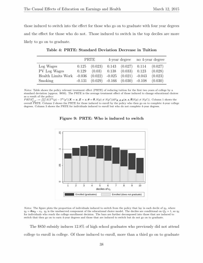
The Causal Effects of Education on Earnings and Health March 12, 2015
those induced to switch into the effect for those who go on to graduate with four year degrees
and the effect for those who do not. Those induced to switch in the top deciles are more
likely to go on to graduate.
Table 4: PRTE: Standard Deviation Decrease in Tuition
PRTE 4-year degree no 4-year degree
Log Wages 0.125 (0.023) 0.143 (0.027) 0.114 (0.027)PV Log Wages 0.129 (0.03) 0.138 (0.033) 0.123 (0.028)Health Limits Work -0.036 (0.022) -0.025 (0.021) -0.043 (0.023)Smoking -0.131 (0.029) -0.166 (0.030) -0.108 (0.030)
Notes: Table shows the policy relevant treatment effect (PRTE) of reducing tuition for the first two years of college by astandard deviation (approx. $850). The PRTE is the average treatment effect of those induced to change educational choicesas a result of the policy:PRTEk
p,p′ :=∫∫∫
E(Tk(p)− Tk(p′)|X = x,Z = z,θ = θ, S(p) 6= S(p′))dFX,Z,θ(x,z,θ|S(p) 6= S(p′)). Column 1 shows the
overall PRTE. Column 2 shows the PRTE for those induced to enroll by the policy who then go on to complete 4-year collegedegrees. Column 3 shows the PRTE for individuals induced to enroll but who do not complete 4-year degrees.
Figure 9: PRTE: Who is induced to switch
0.0
5.1
.15
1 2 3 4 5 6 7 8 9 10
deciles of ε2
Enrolled (graduates) Enrolled (does not graduate)
Notes: The figure plots the proportion of individuals induced to switch from the policy that lay in each decile of η2, whereη2 = θα2 − ν2. η2 is the unobserved component of the educational choice model. The deciles are conditional on Q2 = 1, so η2
for individuals who reach the college enrollment decision. The bars are further decomposed into those that are induced toswitch that then go on to earn 4-year degrees and those that are induced to switch but do not go on to graduate.
The $850 subsidy induces 12.8% of high school graduates who previously did not attend
college to enroll in college. Of those induced to enroll, more than a third go on to graduate
38
The Causal Effects of Education on Earnings and Health March 12, 2015
with a 4 year degree. For outcomes such as smoking, the benefits are larger for those who
graduate with a 4-year degree. The large gains for marginal individuals induced to enroll is
consistent with the literature that finds large psychic costs are necessary to justify why more
individuals do not attend college.
Using the estimated benefits, we can determine if the monetary gains in the present value
of wages at age 18 is greater than the $850 subsidy.65 Given a PRTE of 0.13 for log present
value of wage income, the average gains for those induced to enroll is $36,401. If the subsidy
is given for the first two years of college, then the policy clearly leads to monetary gains for
those induced to enroll. If the subsidy is also offered to those already enrolled, the overall
monetary costs of the subsidy is much larger because it is given to more than 8 students
previously enrolled for each new student induced to enroll (dead weight).
7.2 Boosting Cognitive and Noncognitive Endowments
Using simulation, it is possible to conduct counterfactual policy simulations unrelated to
any particular set of instruments. For example, some early childhood programs have been
shown to have lasting impacts on the cognitive or non-cognitive endowments of low ability
children (see Heckman, Pinto, and Savelyev, 2013). We simulate two policy experiments:
(1) increasing the cognitive endowment of those in the lowest decile and (2) increasing the
non-cognitive endowment of those in the lowest decile.66
The panels of Figure 10 show the average gains for increasing the cognitive or non-cognitive
endowment of those in the lowest decile of each ability. Increased cognition helps individuals
across the board. Increasing socio-emotional endowments has a smaller effect on labor market
outcomes but substantial effects on health.
65However, a limitation of our model is that we can only estimate the monetary costs and do not estimatepsychic costs.
66The details of how these simulations were conducted are presented in Web Appendix A.14. Our modeldoes not address general equilibrium effects of such a change in the endowment distribution.
39
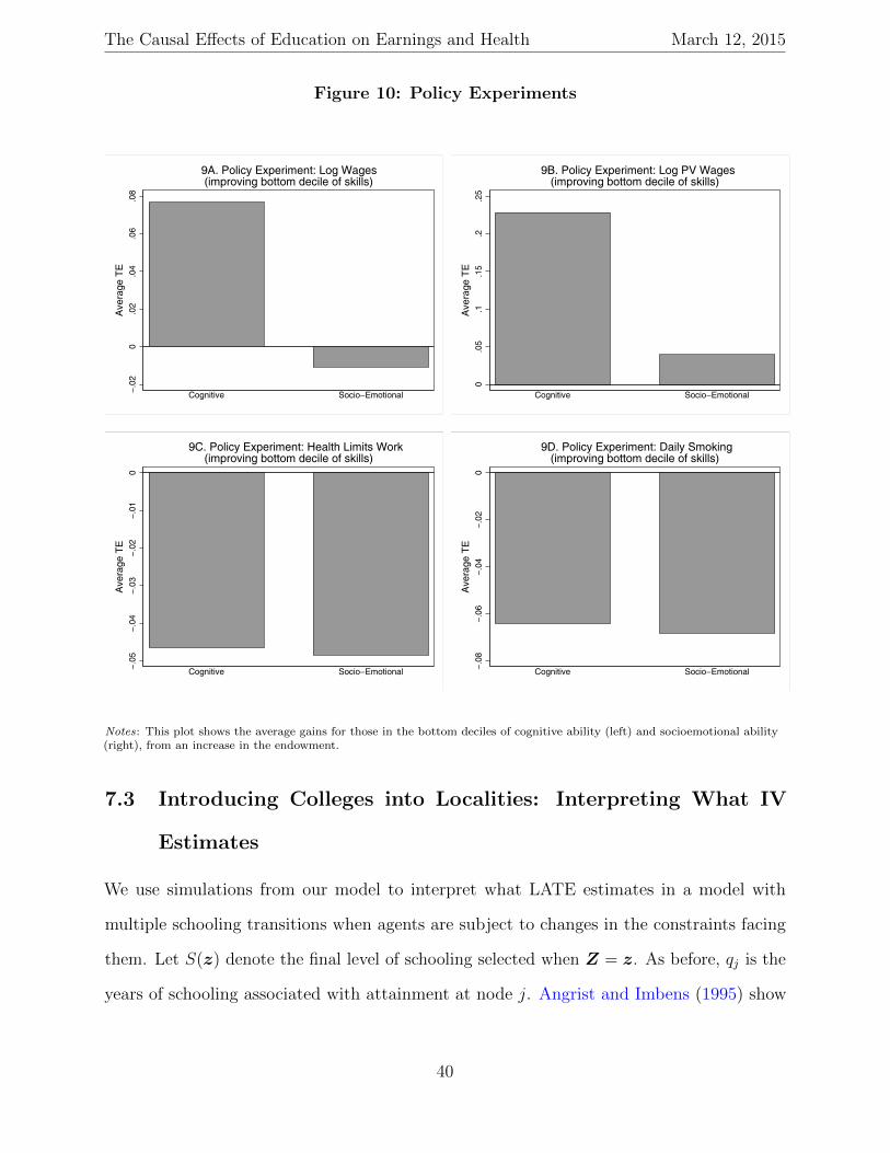
The Causal Effects of Education on Earnings and Health March 12, 2015
Figure 10: Policy Experiments
−.02
0.0
2.0
4.0
6.0
8A
vera
ge T
E
lanoitomE−oicoSevitingoC
9A. Policy Experiment: Log Wages(improving bottom decile of skills)
0.0
5.1
.15
.2.2
5A
vera
ge T
E
lanoitomE−oicoSevitingoC
9B. Policy Experiment: Log PV Wages(improving bottom decile of skills)
−.05
−.04
−.03
−.02
−.01
0A
vera
ge T
E
lanoitomE−oicoSevitingoC
9C. Policy Experiment: Health Limits Work(improving bottom decile of skills)
−.08
−.06
−.04
−.02
0A
vera
ge T
E
lanoitomE−oicoSevitingoC
9D. Policy Experiment: Daily Smoking(improving bottom decile of skills)
Notes: This plot shows the average gains for those in the bottom deciles of cognitive ability (left) and socioemotional ability(right), from an increase in the endowment.
7.3 Introducing Colleges into Localities: Interpreting What IV
Estimates
We use simulations from our model to interpret what LATE estimates in a model with
multiple schooling transitions when agents are subject to changes in the constraints facing
them. Let S(z) denote the final level of schooling selected when Z = z. As before, qj is the
years of schooling associated with attainment at node j. Angrist and Imbens (1995) show
40
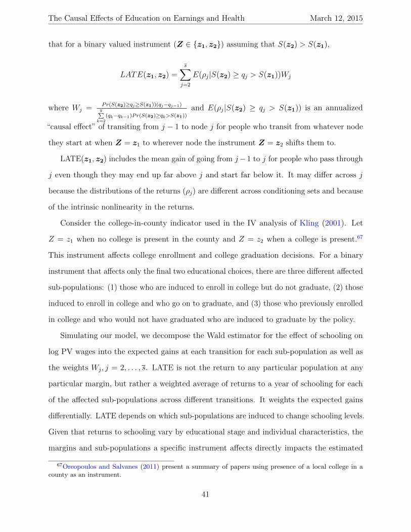
The Causal Effects of Education on Earnings and Health March 12, 2015
that for a binary valued instrument (Z ∈ {z1, z2}) assuming that S(z2) > S(z1),
LATE(z1, z2) =s∑j=2
E(ρj|S(z2) ≥ qj > S(z1))Wj
where Wj =Pr(S(z2)≥qj≥S(z1))(qj−qj−1)s∑
k=2(qk−qk−1)Pr(S(z2)≥qk>S(z1))
and E(ρj|S(z2) ≥ qj > S(z1)) is an annualized
“causal effect” of transiting from j − 1 to node j for people who transit from whatever node
they start at when Z = z1 to wherever node the instrument Z = z2 shifts them to.
LATE(z1, z2) includes the mean gain of going from j−1 to j for people who pass through
j even though they may end up far above j and start far below it. It may differ across j
because the distributions of the returns (ρj) are different across conditioning sets and because
of the intrinsic nonlinearity in the returns.
Consider the college-in-county indicator used in the IV analysis of Kling (2001). Let
Z = z1 when no college is present in the county and Z = z2 when a college is present.67
This instrument affects college enrollment and college graduation decisions. For a binary
instrument that affects only the final two educational choices, there are three different affected
sub-populations: (1) those who are induced to enroll in college but do not graduate, (2) those
induced to enroll in college and who go on to graduate, and (3) those who previously enrolled
in college and who would not have graduated who are induced to graduate by the policy.
Simulating our model, we decompose the Wald estimator for the effect of schooling on
log PV wages into the expected gains at each transition for each sub-population as well as
the weights Wj, j = 2, . . . , s. LATE is not the return to any particular population at any
particular margin, but rather a weighted average of returns to a year of schooling for each
of the affected sub-populations across different transitions. It weights the expected gains
differentially. LATE depends on which sub-populations are induced to change schooling levels.
Given that returns to schooling vary by educational stage and individual characteristics, the
margins and sub-populations a specific instrument affects directly impacts the estimated
67Oreopoulos and Salvanes (2011) present a summary of papers using presence of a local college in acounty as an instrument.
41
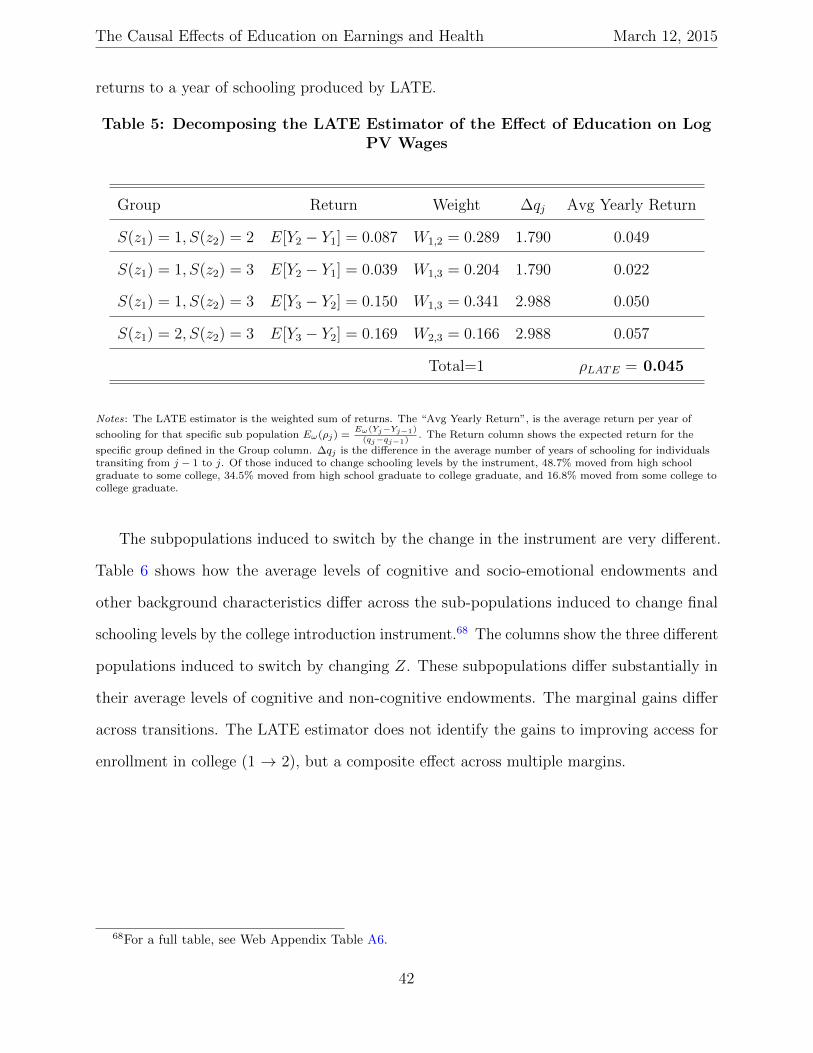
The Causal Effects of Education on Earnings and Health March 12, 2015
returns to a year of schooling produced by LATE.
Table 5: Decomposing the LATE Estimator of the Effect of Education on LogPV Wages
Group Return Weight ∆qj Avg Yearly Return
S(z1) = 1, S(z2) = 2 E[Y2 − Y1] = 0.087 W1,2 = 0.289 1.790 0.049
S(z1) = 1, S(z2) = 3 E[Y2 − Y1] = 0.039 W1,3 = 0.204 1.790 0.022
S(z1) = 1, S(z2) = 3 E[Y3 − Y2] = 0.150 W1,3 = 0.341 2.988 0.050
S(z1) = 2, S(z2) = 3 E[Y3 − Y2] = 0.169 W2,3 = 0.166 2.988 0.057
Total=1 ρLATE = 0.045
Notes: The LATE estimator is the weighted sum of returns. The “Avg Yearly Return”, is the average return per year of
schooling for that specific sub population Eω(ρj) =Eω(Yj−Yj−1)
(qj−qj−1). The Return column shows the expected return for the
specific group defined in the Group column. ∆qj is the difference in the average number of years of schooling for individualstransiting from j − 1 to j. Of those induced to change schooling levels by the instrument, 48.7% moved from high schoolgraduate to some college, 34.5% moved from high school graduate to college graduate, and 16.8% moved from some college tocollege graduate.
The subpopulations induced to switch by the change in the instrument are very different.
Table 6 shows how the average levels of cognitive and socio-emotional endowments and
other background characteristics differ across the sub-populations induced to change final
schooling levels by the college introduction instrument.68 The columns show the three different
populations induced to switch by changing Z. These subpopulations differ substantially in
their average levels of cognitive and non-cognitive endowments. The marginal gains differ
across transitions. The LATE estimator does not identify the gains to improving access for
enrollment in college (1 → 2), but a composite effect across multiple margins.
68For a full table, see Web Appendix Table A6.
42
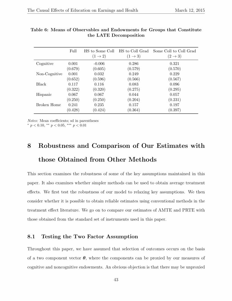
The Causal Effects of Education on Earnings and Health March 12, 2015
Table 6: Means of Observables and Endowments for Groups that Constitutethe LATE Decomposition
Full HS to Some Coll HS to Coll Grad Some Coll to Coll Grad(1→ 2) (1→ 3) (2→ 3)
Cognitive 0.001 -0.006 0.286 0.321(0.679) (0.605) (0.579) (0.570)
Non-Cognitive 0.001 0.032 0.249 0.229(0.652) (0.596) (0.566) (0.567)
Black 0.117 0.116 0.083 0.096(0.322) (0.320) (0.275) (0.295)
Hispanic 0.067 0.067 0.044 0.057(0.250) (0.250) (0.204) (0.231)
Broken Home 0.241 0.235 0.157 0.197(0.428) (0.424) (0.364) (0.397)
Notes: Mean coefficients; sd in parentheses∗ p < 0.10, ∗∗ p < 0.05, ∗∗∗ p < 0.01
8 Robustness and Comparison of Our Estimates with
those Obtained from Other Methods
This section examines the robustness of some of the key assumptions maintained in this
paper. It also examines whether simpler methods can be used to obtain average treatment
effects. We first test the robustness of our model to relaxing key assumptions. We then
consider whether it is possible to obtain reliable estimates using conventional methods in the
treatment effect literature. We go on to compare our estimates of AMTE and PRTE with
those obtained from the standard set of instruments used in this paper.
8.1 Testing the Two Factor Assumption
Throughout this paper, we have assumed that selection of outcomes occurs on the basis
of a two component vector θ, where the components can be proxied by our measures of
cognitive and noncognitive endowments. An obvious objection is that there may be unproxied
43
The Causal Effects of Education on Earnings and Health March 12, 2015
endowments that affect both choices and outcomes that we do not measure.
Cunha and Heckman (2015) estimate a related model using the same data source. They
find that a three factor model explains wages and present value of wages. Two of their factors
correspond to the factors used in this paper. Their third factor improves the fit of the wage
outcome data but does not enter agent decision equations or affect selection or sorting bias.
Our results are consistent with these findings.
In order to test for the presence of a third factor that influences both choices and
outcomes, we test whether the simulated model fits the sample covariances between Y k and
Dj, j = 1, . . . , s, k = 1, . . . , 4. If an important third factor common to both outcome and
choice equations has been omitted, the agreement should be poor. In fact, we find close
agreement.69 Like Cunha and Heckman (2015), we find that adding a third factor that
appears in outcome equations but not choice equations improves goodness of fit, but has no
effect on our estimated treatment effects.70
8.2 Comparisons with Alternative Treatment Effect Estimators
Throughout this paper we have exploited the assumption of conditional independence of
outcomes and choices given X,Z,θ. This raises the question of how similar our results would
be if we had used simple matching methods that also control for θ,X,Z.71 We estimate
Bartlett factor scores based on our measures using standard statistical software.72 Using
these extracted factors, we estimate average treatment effects using (a) Linear regression
(with and without factors) and (b) Matching. Table 8 presents our estimates. All models are
estimated for individuals who attain each decision node (Qj = 1) and include those who may
go on to attain further education in order to make the alternative models comparable to our
ATE estimate that includes continuation values.
The first three columns show estimates from linear models. The first two columns
69See Web Appendix A.15 and Table A38.70See Web Appendix A.15.71OLS is a version of matching.72See Bartlett (1937, 1938).
44
The Causal Effects of Education on Earnings and Health March 12, 2015
introduce schooling by using dummy shifts in intercepts. The first column uses measures
of cognitive and noncognitive endowments directly, while the second column includes the
extracted factor scores. The third column allows loadings on covariates and factor scores to
vary by schooling level.73
The fourth and fifth columns show estimates from matching using the Bartlett factor
scores previously described as well as an index of covariates. The fourth column shows results
from nearest neighbor matching using the 3 nearest neighbors. The fifth column shows results
from propensity score matching using the estimated probability of the educational decision
as the propensity score.74
The estimates differ greatly from the OLS estimates obtained without any adjustment for
θ. Controlling for ability has substantial effects on the estimated average treatment effects.
Across schooling nodes, all of the other estimates are roughly “within the ball park” of the
estimates produced from our model, provided that we control for θ. This is good news for
applied economists mainly interested in using simple methods to estimate average treatment
effects. However, these simple methods are powerless in estimating AMTE and PRTE or
answering many of the other questions addressed in this paper.75
8.3 Comparison of Estimates from Our Model with Those from
IV
Table 8 compares the AMTE and PRTE parameters generated from our model with standard
estimates based on the widely used instruments of Table 1. The IV estimates are not close
to our estimates of the interpretable policy relevant treatment effects or average marginal
treatment effects. The IV estimates vary substantially based on which instruments we use and
73See Section A.16.3 for details on these estimators.74Precise specifications of the estimating equations are presented in Web Appendix A.16.75Table A73 of the Web Appendix compares OLS estimates of direct effects and continuation values with
our model estimates. The OLS estimates are “within ballpark” for smoking and health limits work, but theyare wide of the mark for wages and PV wages.
45
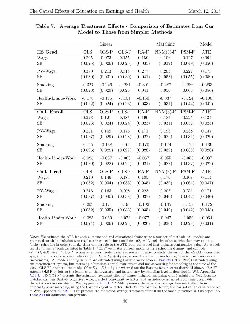
The Causal Effects of Education on Earnings and Health March 12, 2015
Table 7: Average Treatment Effects - Comparison of Estimates from OurModel to Those from Simpler Methods
Linear Matching Model
HS Grad. OLS OLS-P OLS-F RA-F NNM(3)-F PSM-F ATE
Wages 0.205 0.073 0.155 0.159 0.106 0.127 0.094SE (0.025) (0.026) (0.025) (0.035) (0.039) (0.049) (0.056)
PV-Wage 0.380 0.213 0.318 0.277 0.203 0.227 0.173SE (0.030) (0.031) (0.030) (0.041) (0.053) (0.055) (0.059)
Smoking -0.327 -0.246 -0.281 -0.301 -0.287 -0.286 -0.263SE (0.028) (0.029) 0.028 0.041 0.056 0.068 (0.056)
Health-Limits-Work -0.178 -0.115 -0.151 -0.150 -0.037 -0.124 -0.108SE (0.022) (0.024) (0.023) (0.033) (0.031) (0.044) (0.042)
Coll. Enroll OLS OLS-P OLS-F RA-F NNM(3)-F PSM-F ATE
Wages 0.223 0.121 0.186 0.190 0.185 0.225 0.134SE (0.023) (0.024) (0.024) (0.023) (0.031) (0.032) (0.025)
PV-Wage 0.221 0.109 0.176 0.171 0.198 0.238 0.137SE (0.027) (0.029) (0.028) (0.027) (0.029) (0.031) (0.029)
Smoking -0.177 -0.138 -0.165 -0.170 -0.174 -0.175 -0.139SE (0.026) (0.028) (0.027) (0.028) (0.032) (0.033) (0.028)
Health-Limits-Work -0.085 -0.037 -0.066 -0.057 -0.055 -0.056 -0.037SE (0.020) (0.022) (0.021) (0.021) (0.022) (0.037) (0.022)
Coll. Grad OLS OLS-P OLS-F RA-F NNM(3)-F PSM-F ATE
Wages 0.210 0.146 0.184 0.185 0.176 0.108 0.114SE (0.032) (0.034) (0.033) (0.035) (0.039) (0.061) (0.037)
PV-Wage 0.243 0.163 0.208 0.228 0.207 0.251 0.171SE (0.037) (0.040) (0.038) (0.037) (0.040) (0.042) (0.040)
Smoking -0.209 -0.171 -0.195 -0.192 -0.145 -0.157 -0.172SE (0.032) (0.035) (0.033) (0.035) (0.040) (0.042) (0.043)
Health-Limits-Work -0.085 -0.069 -0.078 -0.077 -0.047 -0.059 -0.064SE (0.024) (0.026) (0.025) (0.026) (0.030) (0.028) (0.031)
Notes: We estimate the ATE for each outcome and and educational choice using a number of methods. All models areestimated for the population who reaches the choice being considered (Qj = 1), inclusive of those who then may go on tofurther schooling in order to make them comparable to the ATE from our model that includes continuation value. All modelsuse the full set of controls listed in Table 1. “OLS” estimates a linear model using a schooling dummy, and controls(Y = Dj +Xβ + ε). “OLS-P” estimates a linear model using a schooling dummy, controls, the sum of the ASVAB scores used,gpa, and an indicator of risky behavior (Y = Dj +Xβ +Aγ + ε, where A are the proxies for cognitive and socio-emotionalendowments). All models ending in ”-F” are estimated using Bartlett factor scores ( Bartlett (1937, 1938)) estimated usingour measurement system, but assuming a bivariate normal distribution and not accounting for schooling at the time of thetest. “OLS-F” estimates the model (Y = Dj +Xβ + θγ + ε where θ are the Bartlett factor scores described above. “RA-F”extends OLS-F by letting the loadings on the covariates and factors vary by schooling level as described in Web AppendixA.16.3. “NNM(3)-F” presents the estimated treatment effect of nearest-neighbor matching with 3 neighbors. Neighbors arematched on their Bartlett cognitive factor, Bartlett non-cognitive factor, and an index constructed from their observablecharacteristics as described in Web Appendix A.16.1. “PSM-F” presents the estimated average treatment effect frompropensity score matching, using the Bartlett cognitive factor, Bartlett non-cognitive factor, and control variables as describedin Web Appendix A.16.2. “ATE” presents the estimated average treatment effect from the model presented in this paper. SeeTable A54 for additional comparisons.
46
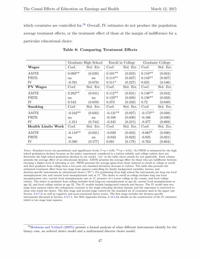
The Causal Effects of Education on Earnings and Health March 12, 2015
which covariates are controlled for.76 Overall, IV estimates do not produce the population
average treatment effects, or the treatment effect of those at the margin of indifference for a
particular educational choice.
Table 8: Comparing Treatment Effects
Graduate High School Enroll in College Graduate College
Wages Coef. Std. Err. Coef. Std. Err. Coef. Std. Err.
AMTE 0.093** (0.028) 0.101** (0.023) 0.110** (0.034)PRTE na na 0.114** (0.027) 0.143** (0.027)IV -0.761 (0.678) 0.511* (0.227) 0.025 (0.546)
PV Wages Coef. Std. Err. Coef. Std. Err. Coef. Std. Err.
AMTE 0.282** (0.041) 0.112** (0.031) 0.146** (0.042)PRTE na na 0.123** (0.028) 0.138** (0.033)IV 0.542 (0.659) 0.373 (0.233) 0.72 (0.640)
Smoking Coef. Std. Err. Coef. Std. Err. Coef. Std. Err.
AMTE -0.242** (0.033) -0.131** (0.027) -0.173** (0.038)PRTE na na -0.108 (0.030) -0.166 (0.030)IV -1.311 (0.744) -0.345 (0.215) -0.377 (0.693)
Health Limits Work Coef. Std. Err. Coef. Std. Err. Coef. Std. Err.
AMTE -0.110** (0.031) -0.029 (0.022) -0.067* (0.030)PRTE na na -0.043 (0.023) -0.025 (0.021)IV -0.560 (0.577) 0.081 (0.178) -0.763 (0.664)
Notes: Standard errors (in parenthesis) and significance levels (*=p < 0.05, **=p < 0.01). No PRTE is estimated for the highschool graduation decision because as the policy experiment considered is a tuition subsidy and college tuition does notdetermine the high school graduation decision in our model. “na” in the table above stands for not applicable. Each columnpresents the average effect of an educational decision. AMTE presents the average effect for those who are indifferent betweenchoosing a higher level of schooling or not. PRTE presents the average gains from those induced to enroll in college or enrolland then graduate from college from a two-year one standard deviation decrease in tuition. The table also presents theestimated treatment effect from two stage least squares controlling for family background variables, factors, anddecision-specific instruments by educational choice (“IV”). For graduating from high school the instruments are long run localunemployment rate and current local unemployment rate at 17. The choice to enroll in college includes long run localunemployment rate, current local unemployment rate at 17, presence of a 4-year college in the county, and local collegetuition. The choice to graduate from college includes local long-run unemployment at age 22, current local unemployment atage 22, and local college tuition at age 22. The IV models include background controls and factors. The IV model uses twostage least squares where the endogenous covariate is the single schooling decision dummy and the regression is restricted tothose who reach the choice. The first stage and second stage control for the standard set of covariates used in the paper (seeSection A.8.7.2) as well as cognitive and socio-emotional factor scores. The first stage includes the decision specificinstruments discussed in Section A.8.7.4. See Web Appendix Section A.16.4 for details on the construction of the IV estimatorwhich is two stage least squares.
76Heckman and Vytlacil (2007b) present a formal analysis of what different instruments identify for thebinary case, an ordered choice model and a multinomial discrete choice model.
47
The Causal Effects of Education on Earnings and Health March 12, 2015
9 Summary and Conclusion
Gary Becker’s seminal research on human capital launched a large and active industry on
estimating causal effects and rates of return to schooling. Multiple methodological approaches
have been used to secure estimates ranging from reduced form treatment effect methods to
fully structural methods. Each methodology has its benefits and limitations.
This paper develops and estimates a robust dynamic causal model of schooling and its
consequences for earnings, health and healthy behaviors. The model recognizes the sequential
dynamic nature of educational decisions. We borrow features from both the reduced form
treatment effect literature and the structural literature. Our estimated model passes a variety
of goodness of fit and model specification tests.
We allow agents to be irrational and myopic in making schooling decisions. Hence we can
use our model to test some of the maintained assumptions in the dynamic discrete choice
literature on schooling.
We use our dynamic choice model to interpret what IV estimates and to identify the sets
of agents affected by various instruments. We estimate causal effects from multiple levels of
schooling rather than the binary comparisons typically featured in the literature on treatment
effects and in many structural papers.77
By estimating a sequential model of schooling in a unified framework, we are able analyze
the ex post returns to education for people at different margins of choice and analyze a variety
of interesting policy counterfactuals. We are able to characterize who benefits from education
across a variety of market and nonmarket outcomes.
The early literature on human capital ignored the dynamics of schooling choices. We
decompose these benefits into direct components and indirect components arising from
continuation values. We estimate substantial continuation value components especially for
high ability individuals. For them, schooling opens up valuable options for future schooling.
Standard estimates of the benefits of education based only on direct components underestimate
77See, e.g., Willis and Rosen (1979).
48
The Causal Effects of Education on Earnings and Health March 12, 2015
the full benefits of education.
Without imposing rationality, we nonetheless find evidence consistent with it. We find
positive sorting into schooling based on gains, especially for higher schooling levels. Schooling
has strong causal effects on earnings, health and healthy behaviors even though we also find
strong evidence of ability bias at all levels of schooling. Both cognitive and noncognitive
endowments affect schooling choices and outcomes for each level of schooling.
We test numerous implications of the Becker - Chiswick - Mincer model (1) and find
substantial evidence against it. The distributions of annualized returns differ across schooling
levels. The returns are also far from perfectly correlated across schooling transitions and
some are even negatively correlated. The correlation of returns and schooling attained differs
greatly across schooling levels. There is heterogeneity in the effects of schooling across levels
of schooling for the same person and heterogeneity in the effects of extra schooling across
persons.
We link the structural and matching literatures using conditional independence assump-
tions. We investigate how simple methods used in the treatment effect literature perform
in estimating average treatment effects. They roughly approximate our model estimates
provided analysts condition on endowments of cognitive and noncognitive skills, and correct
for measurement error in the proxies. However, these simple methods do not identify the
treatment effects for persons at the margins of different choices, the policy relevant treatment
effects, or the continuation values analyzed in this paper. Estimates from IV model are very
different from the economically interpretable and policy relevant estimates produced from
our model.
We deepen understanding of LATE by identifying the groups affected by variations in
instruments and policies. We compare our estimates to those estimated by LATE and use
our model to decompose the LATE estimator into economically interpretable components.
Our analysis is broadly consistent with the pioneering analysis of Becker (1964) but
enriches it. The early research on human capital was casual about agent heterogeneity. It
49
The Causal Effects of Education on Earnings and Health March 12, 2015
ignored selection bias and comparative advantage in schooling. We quantify the magnitude and
sources of selection bias. We find evidence of both ability bias and sorting bias (comparative
advantage). Nonetheless, we find strong causal effects of education at most margins for most
outcomes.
Our findings thus support the basic insights of Becker (1964). Schooling has strong causal
effects on market and nonmarket outcomes. Both cognitive and noncognitive endowments
affect schooling choices and outcomes. People tend to sort into schooling based on gains.
50
The Causal Effects of Education on Earnings and Health March 12, 2015
References
Abbring, J. H., and J. J. Heckman (2007): “Econometric Evaluation of Social Programs,
Part III: Distributional Treatment Effects, Dynamic Treatment Effects, Dynamic Discrete
Choice, and General Equilibrium Policy Evaluation,” in Handbook of Econometrics, ed. by
J. Heckman, and E. Leamer, vol. 6B, pp. 5145–5303. Elsevier, Amsterdam.
Adda, J., and R. W. Cooper (2003): Dynamic Economics: Quantitative Methods and
Applications. The MIT Press, Cambridge, Mass.
Aguirregabiria, V. (2010): “Another look at the identification of dynamic discrete decision
processes: An application to retirement behavior,” Journal of Business & Economic
Statistics, 28(2), 201–218.
Almlund, M., A. Duckworth, J. J. Heckman, and T. Kautz (2011): “Personality
Psychology and Economics,” in Handbook of the Economics of Education, ed. by E. A.
Hanushek, S. Machin, and L. Woßmann, vol. 4, pp. 1–181. Elsevier, Amsterdam.
Altonji, J. G. (1993): “The Demand for and Return to Education When Education
Outcomes are Uncertain,” Journal of Labor Economics, 11(1), 48–83.
Angrist, J. D., and G. W. Imbens (1995): “Two-Stage Least Squares Estimation of
Average Causal Effects in Models with Variable Treatment Intensity,” Journal of the
American Statistical Association, 90(430), 431–442.
Angrist, J. D., and J.-S. Pischke (2009): Mostly Harmless Econometrics: An Empiricist’s
Companion. Princeton University Press, Princeton.
Bartlett, M. S. (1937): “The Statistical Conception of Mental Factors,” British Journal
of Psychology: General Section, 28(1), 97–104.
Bartlett, M. S. (1938): “Methods of Estimating Mental Factors,” Nature, 141(3570),
609–610.
51
The Causal Effects of Education on Earnings and Health March 12, 2015
Becker, G. S. (1962): “Irrational Behavior and Economic Theory,” Journal of Political
Economy, 70, 1–13.
Becker, G. S. (1964): Human Capital: A Theoretical and Empirical Analysis, With Special
Reference to Education. National Bureau of Economic Research, New York.
Becker, G. S. (1967): “Human Capital and the Personal Distribution of Income: An
Analytical Approach,” Woytinsky Lecture no. 1. Ann Arbor: University of Michigan,
Institute of Public Administration.
(1991): A Treatise on the Family. Harvard University Press, Cambridge, MA,
enlarged edn.
Becker, G. S., and B. R. Chiswick (1966): “Education and the Distribution of Earnings,”
American Economic Review, 56(1/2), 358–369.
Blevins, J. R. (2014): “Nonparametric Identification of Dynamic Decision Processes with
Discrete and Continuous Choices,” Quantitative Economics, 5(3), 531–554.
Borghans, L., A. L. Duckworth, J. J. Heckman, and B. ter Weel (2008): “The
Economics and Psychology of Personality Traits,” Journal of Human Resources, 43(4),
972–1059.
Cameron, S. V., and J. J. Heckman (1993): “The Nonequivalence of High School
Equivalents,” Journal of Labor Economics, 11(1, Part 1), 1–47.
(2001): “The Dynamics of Educational Attainment for Black, Hispanic, and White
Males,” Journal of Political Economy, 109(3), 455–499.
Cameron, S. V., and C. Taber (2004): “Estimation of Educational Borrowing Constraints
Using Returns to Schooling,” Journal of Political Economy, 112(1), 132–182.
52
The Causal Effects of Education on Earnings and Health March 12, 2015
Card, D. (1999): “The Causal Effect of Education on Earnings,” in Handbook of Labor
Economics, ed. by O. Ashenfelter, and D. Card, vol. 5, pp. 1801–1863. North-Holland, New
York.
(2001): “Estimating the Return to Schooling: Progress on Some Persistent Econo-
metric Problems,” Econometrica, 69(5), 1127–1160.
(2012): “Earnings, Schooling, and Ability Revisited,” in 35th Anniversary Retro-
spective (Research in Labor Economics), ed. by S. Polachek, and K. Tatsiramos, vol. 35, pp.
111–136. Emerald Group Publishing Limited.
Carneiro, P., K. Hansen, and J. J. Heckman (2003): “Estimating Distributions of
Treatment Effects with an Application to the Returns to Schooling and Measurement of the
Effects of Uncertainty on College Choice,” International Economic Review, 44(2), 361–422.
Carneiro, P., J. J. Heckman, and E. J. Vytlacil (2010): “Evaluating Marginal Policy
Changes and the Average Effect of Treatment for Individuals at the Margin,” Econometrica,
78(1), 377–394.
Carneiro, P., J. J. Heckman, and E. J. Vytlacil (2011): “Estimating Marginal
Returns to Education,” American Economic Review, 101(6), 2754–2781.
Carneiro, P., C. Meghir, and M. Parey (2013): “Maternal Education, Home Envi-
ronments, and the Development of Children and Adolescents,” Journal of the European
Economic Association, 11(s1), 123–160.
Cawley, J., K. Conneely, J. J. Heckman, and E. J. Vytlacil (1997): “Cognitive
Ability, Wages and Meritocracy,” in Intelligence, Genes, and Success : Scientists Respond
to The Bell Curve, ed. by B. Devlin, S. Fienberg, D. Resnick, and K. Roeder, pp. 179–192.
Springer, New York.
Comay, Y., A. Melnik, and M. A. Pollatschek (1973): “The Option Value of Education
53
The Causal Effects of Education on Earnings and Health March 12, 2015
and the Optimal Path for Investment in Human Capital,” International Economic Review,
14(2), 421–435.
Cunha, F., and J. J. Heckman (2015): “Decomposing Trends in Inequality in Earnings
into Forcastable and Uncertain Components* Lazear Festschrift,” .
Cutler, D. M., and A. Lleras-Muney (2010): “Understanding Differences in Health
Behaviors by Education,” Journal of Health Economics, 29(1), 1–28.
Eckstein, Z., and K. I. Wolpin (1989): “The Specification and Estimation of Dynamic
Stochastic Discrete Choice Models: A Survey,” Journal of Human Resources, 24(4), 562–
598.
Eisenhauer, P., J. Heckman, and S. Mosso (2015): “Estimation of Dynamic Dis-
crete Choice Models by Maximum Likelihood and the Simulated Method of Moments,”
Forthcoming, International Economic Review.
Eisenhauer, P., J. J. Heckman, and E. J. Vytlacil (2015): “Generalized Roy Model
and Cost-Benefit Analysis of Social Programs,” Forthcoming, Journal of Political Economy.
Geweke, J., and M. Keane (2001): “Computationally Intensive Methods for Integration
in Econometrics,” in Handbook of Econometrics, ed. by J. J. Heckman, and E. Leamer,
vol. 5, pp. 3463–3568. North-Holland, New York.
Griliches, Z. (1977): “Estimating the Returns to Schooling: Some Econometric Problems,”
Econometrica, 45(1), 1–22.
Grossman, M. (2000): “The Human Capital Model,” in Handbook of Health Economics, ed.
by A. J. Culyer, and J. P. Newhouse, vol. 1, pp. 347–408. Elsevier, Amsterdam.
Haavelmo, T. (1943): “The Statistical Implications of a System of Simultaneous Equations,”
Econometrica, 11(1), 1–12.
54
The Causal Effects of Education on Earnings and Health March 12, 2015
Hansen, L. P., and T. J. Sargent (1980): “Formulating and Estimating Dynamic Linear
Rational Expectations Models,” Journal of Economic Dynamics and Control, 2(1), 7–46.
Heckman, J., S. Schennach, and B. Williams (2013): “Matching on Proxy Variables,”
University of Chicago.
Heckman, J. J. (1981): “The Empirical Content of Alternative Models of Labor Earnings,”
Unpublished manuscript, University of Chicago, Department of Economics.
(2010): “Building Bridges Between Structural and Program Evaluation Approaches
to Evaluating Policy,” Journal of Economic Literature, 48(2), 356–398.
Heckman, J. J., P. Carneiro, and E. Vytlacil (2011): “Estimating Marginal Returns
to Education,” American Economic Review, 101(6), 2754–2871.
Heckman, J. J., J. E. Humphries, and T. Kautz (2014): “The Economic and Social
Benefits of GED Certification,” in The Myth of Achievement Tests: The GED and the
Role of Character in American Life, ed. by J. J. Heckman, J. E. Humphries, and T. Kautz,
chap. 5, pp. 171–267. University of Chicago Press, Chicago.
Heckman, J. J., H. Ichimura, and P. E. Todd (1998): “Matching as an Econometric
Evaluation Estimator,” Review of Economic Studies, 65(2), 261–294.
Heckman, J. J., L. J. Lochner, and P. E. Todd (2006): “Earnings Functions, Rates of
Return and Treatment Effects: The Mincer Equation and Beyond,” in Handbook of the
Economics of Education, ed. by E. A. Hanushek, and F. Welch, vol. 1, chap. 7, pp. 307–458.
Elsevier, Amsterdam.
Heckman, J. J., and R. Pinto (2015): “Causal Analysis after Haavelmo,” Econometric
Theory, 31(01), 115–151.
55

The Causal Effects of Education on Earnings and Health March 12, 2015
Heckman, J. J., R. Pinto, and P. A. Savelyev (2013): “Understanding the Mecha-
nisms Through Which an Influential Early Childhood Program Boosted Adult Outcomes,”
American Economic Review, 103(6), 2052–86.
Heckman, J. J., S. Schennach, and B. Williams (2011): “Matching with Error-Laden
Covariates,” Unpublished manuscript, University of Chicago, Department of Economics.
Heckman, J. J., J. Stixrud, and S. Urzua (2006): “The Effects of Cognitive and
Noncognitive Abilities on Labor Market Outcomes and Social Behavior,” Journal of Labor
Economics, 24(3), 411–482.
Heckman, J. J., and E. J. Vytlacil (1999): “Local Instrumental Variables and Latent
Variable Models for Identifying and Bounding Treatment Effects,” Proceedings of the
National Academy of Sciences, 96(8), 4730–4734.
(2005): “Structural Equations, Treatment Effects and Econometric Policy Evalua-
tion,” Econometrica, 73(3), 669–738.
(2007a): “Econometric Evaluation of Social Programs, Part I: Causal Models,
Structural Models and Econometric Policy Evaluation,” in Handbook of Econometrics, ed.
by J. Heckman, and E. Leamer, vol. 6B, pp. 4779–4874. Elsevier, Amsterdam.
(2007b): “Econometric Evaluation of Social Programs, Part II: Using the Marginal
Treatment Effect to Organize Alternative Economic Estimators to Evaluate Social Programs
and to Forecast Their Effects in New Environments,” in Handbook of Econometrics, ed. by
J. Heckman, and E. Leamer, vol. 6B, chap. 71, pp. 4875–5143. Elsevier, Amsterdam.
Kane, T. J., and C. E. Rouse (1993): “Labor Market Returns to Two- and Four-Year
Colleges: Is a Credit a Credit and Do Degrees Matter?,” 1993 working paper, 4268, National
Bureau of Economic Research.
Keane, M. P., and K. I. Wolpin (1997): “The Career Decisions of Young Men,” Journal
of Political Economy, 105(3), 473–522.
56
The Causal Effects of Education on Earnings and Health March 12, 2015
Kling, J. R. (2001): “Interpreting Instrumental Variables Estimates of the Returns to
Schooling,” Journal of Business and Economic Statistics, 19(3), 358–364.
Lochner, L. (2011): “Non-Production Benefits of Education: Crime, Health, and Good
Citizenship,” Working Paper 16722, National Bureau of Economic Research.
McMahon, W. W. (2000): “Externalities, non-market effects, and trends in returns to
educational investments,” in The Appraisal of Investments in Educational Facilities, pp.
51–83. European Investment Bank/OECD, Paris.
(2009): Higher Learning, Greater Good. Johns Hopkins University Press, Baltimore.
Mincer, J. (1974): Schooling, Experience and Earnings. Columbia University Press for
National Bureau of Economic Research, New York.
Oreopoulos, P., and U. Petronijevic (2013): “Making College Worth It: A Review of
Research on the Returns to Higher Education,” Working Paper 19053, National Bureau of
Economic Research, Cambridge.
Oreopoulos, P., and K. G. Salvanes (2011): “Priceless: The Nonpecuniary Benefits of
Schooling,” Journal of Economic Perspectives, 25(1), 159–184.
Quandt, R. E. (1958): “The Estimation of the Parameters of a Linear Regression System
Obeying Two Separate Regimes,” Journal of the American Statistical Association, 53(284),
873–880.
(1972): “A New Approach to Estimating Switching Regressions,” Journal of the
American Statistical Association, 67(338), 306–310.
Rust, J. (1994): “Structural Estimation of Markov Decision Processes,” in Handbook of
Econometrics, Volume, ed. by R. Engle, and D. McFadden, pp. 3081–3143. North-Holland,
New York.
57
The Causal Effects of Education on Earnings and Health March 12, 2015
Schennach, S., H. White, and K. Chalak (2012): “Local indirect least squares and
average marginal effects in nonseparable structural systems,” Journal of Econometrics,
166(2), 282–302.
Vytlacil, E. J. (2002): “Independence, Monotonicity, and Latent Index Models: An
Equivalence Result,” Econometrica, 70(1), 331–341.
Weisbrod, B. A. (1962): “Education and Investment in Human Capital,” Journal of
Political Economy, 70(5, Part 2: Investment in Human Beings), 106–123.
White, H., and K. Chalak (2009): “Settable Systems: An Extension of Pearl’s Causal
Model with Optimization, Equilibrium, and Learning,” Journal of Machine Learning
Research, 10, 1759–1799.
Willis, R. J., and S. Rosen (1979): “Education and Self-Selection,” Journal of Political
Economy, 87(5, Part 2), S7–S36.
58