The Causal Effect of Education on Health:

What is the Role of Health Behaviors?

Giorgio Brunello, Margherita Fort, Nicole Schneeweis, Rudolf Winter-Ebmer

280

Reihe Ökonomie

Economics Series

280

Reihe Ökonomie

Economics Series

The Causal Effect of Education on Health:

What is the Role of Health Behaviors?

Giorgio Brunello, Margherita Fort, Nicole Schneeweis, Rudolf Winter-Ebmer

December 2011

Institut für Höhere Studien (IHS), Wien Institute for Advanced Studies, Vienna

Contact: Giorgio Brunello Department of Economics University of Padua Via del Santo, 33 I-35121 Padov, Italy email: giorgio.brunello@unipd.it Margherita Fort Department of Economics University of Bologna Piazza Scaravilli 2 I-40126 Bologna, Italy email: margherita.fort@unibo.it Nicole Schneeweis Department of Economics Johannes Kepler University Altenberger Str. 69 A-4040 Linz-Auhof, Austria email: nicole.schneeweis@jku.at Rudolf Winter-Ebmer Department of Economics Johannes Kepler University Altenberger Str. 69 A-4040 Linz-Auhof, Austria email: rudolf.winterebmer@jku.at and Institute for Advanced Studies, Vienna; CEPR; IZA

Founded in 1963 by two prominent Austrians living in exile – the sociologist Paul F. Lazarsfeld and the

economist Oskar Morgenstern – with the financial support from the Ford Foundation, the Austrian

Federal Ministry of Education and the City of Vienna, the Institute for Advanced Studies (IHS) is the

first institution for postgraduate education and research in economics and the social sciences in

Austria. The Economics Series presents research done at the Department of Economics and Finance

and aims to share “work in progress” in a timely way before formal publication. As usual, authors bear

full responsibility for the content of their contributions.

Das Institut für Höhere Studien (IHS) wurde im Jahr 1963 von zwei prominenten Exilösterreichern –

dem Soziologen Paul F. Lazarsfeld und dem Ökonomen Oskar Morgenstern – mit Hilfe der Ford-

Stiftung, des Österreichischen Bundesministeriums für Unterricht und der Stadt Wien gegründet und ist

somit die erste nachuniversitäre Lehr- und Forschungsstätte für die Sozial- und Wirtschafts-

wissenschaften in Österreich. Die Reihe Ökonomie bietet Einblick in die Forschungsarbeit der

Abteilung für Ökonomie und Finanzwirtschaft und verfolgt das Ziel, abteilungsinterne

Diskussionsbeiträge einer breiteren fachinternen Öffentlichkeit zugänglich zu machen. Die inhaltliche

Verantwortung für die veröffentlichten Beiträge liegt bei den Autoren und Autorinnen.

Abstract We study the contribution of health-related behaviors to the health-education gradient by

distinguishing between short-run and long-run mediating effects:while in the former only

current or lagged behaviors are taken into account, in the latter we consider the entire history

of behaviors. We use an empirical approach that addresses the endogeneity of education

and behaviors in the health production function. Focusing on self-reported poor health as our

health out-come, we find that education has a protective effect for European males and

females aged 50+. We also find that the mediating effects of health behaviors - measured by

smoking, drinking, exercising and the body mass index – account in the short run for 17% to

31% and in the long run for 23% to 45% of the entire effect of education on health,

depending on gender.

Keywords Health, education, health behaviors, Europe

JEL Classification I1, I12, I21

Comments

We would like to thank the participants to seminars in Bologna, Bressanone, Catanzaro, Firenze,

Hangzhou, Linz, Munich, Nurnberg, Padova, Regensburg, and Wurzburg and especially our

discussant, Lance Lochner, for his very detailed comments and suggestions on an earlier version of the

paper. We acknowledge the nancial support of Fondazione Cariparo, MIUR- FIRB 2008 project

RBFR089QQC-003-J31J10000060001 and the Austrian Science Fund (FWF: S103 The Austrian

Center for Labor Economics and the Analysis of the Welfare State). The SHARE data collection has

been primarily funded by the European Commission through the 5th, 6th and 7th framework

programme, as well as by the U.S. National Institute on Aging and other national Funds. The usual

disclaimer applies.

Contents

1 Introduction 1

2 Review of the Literature 3

3 The Contribution of Health Behaviors to the Education Gradient 4 3.1 The History of Behaviors ............................................................................................ 5

3.2 Estimating the Short-Run and Long-Run Mediating Effects ....................................... 7

4 The Empirical Strategy 8 4.1 The Card-Rothstein approach .................................................................................. 10

4.2 The IV approach ....................................................................................................... 12

5 Data 12

6 Results 15 6.1 Baseline Estimates of the Reduced Form and Dynamic Health Equations .............. 15

6.2 IV Estimates of the Reduced Form Health Equation ................................................ 18

6.3 IV and ADS Results Compared ................................................................................ 19

6.4 Robustness Checks .................................................................................................. 20

7 Conclusions 21

8 Tables 23

References 30

Appendix A: An Illustrative Model A.1

Appendix B: Synthetic Indicators for Parental Background B.1

Appendix C: Educational Reforms in Europe C.1

1 Introduction

The relationship between education and health - the ”education gradient” - is widely

studied. There is abundant evidence that a gradient exists (Cutler and Lleras-Muney,

2010). Yet less is known as to why education might be related to health. In this

paper we explore the contribution of health-related behaviors (shortly, behaviors) -

which we measure with smoking, drinking, exercising and the body mass index - to

the education gradient. To do so, we decompose the gradient into two parts: a) the

part mediated by health behaviors; b) a residual, which includes for instance stress

reduction, better decision making, better information collection, healthier employment

and better neighborhoods (Lochner, 2011).1

We are not the first to investigate the mediating role of health behaviors. Our

contribution is two-fold: first, we distinguish between short-run and long-run mediating

effects. Typically, the empirical literature considers only the former and focuses either

on current behaviors or on behaviors in the immediate past, thereby ignoring the

contribution of the previous history of behaviors. By ignoring this history, short-run

mediating effects are likely to underestimate the overall mediating effect of behaviors

whenever there is some persistence in the health status. Second, as recently pointed

out by Lochner (2011), a problem with the existing empirical literature is that most

contributions fail to address the endogeneity of education and behaviors in health

regressions and therefore ignore that there are possibly many confounding factors

which influence both education and behaviors, on the one hand, and health outcomes,

on the other hand. While some studies have dealt with endogenous education, our

approach is novel because we address the endogeneity of both education and behaviors

in the health production function, and therefore can give a causal interpretation to

our estimates.

Our identification strategy - based on the work by Card and Rothstein (2007) -

allows us to estimate average education effects for an individual randomly picked from

the population. Using a cross-country dataset, where we have a rich set of parental

and early life information, this strategy combines selection on observables and fixed

effects assumptions to estimate the parameters of both a dynamic health equation,

which depends on education and lagged health behaviors, and a static health equation,

where health depends only on education. The effect of education on health in the

second equation is the education gradient (shortly, the gradient), i.e. the total effect of

education on health that results from both mediated and residual effects of education.

We compare the estimates of the gradient obtained following the strategy outlined

above with those obtained with a completely different methodology, instrumental vari-

1The residual also includes the contribution of unmeasured behaviors.

1

ables (IV) estimation, where the key exogenous variation is provided by the changes

in compulsory schooling laws across countries and birth cohorts. While the IV strat-

egy generates causal estimates that are internally valid for individuals affected by

mandatory schooling laws (compliers), it cannot be used for the decomposition of the

education gradient because of the lack of valid and relevant instruments for behaviors.

We apply this approach to a multi-country data set, which includes 12 European

countries (Austria, Belgium, Denmark, England, France, Germany, Greece, Italy, the

Netherlands, Spain, Sweden and Switzerland) and has information on education, health

and health behaviors for a sample of males and females aged 50+. By focusing on older

individuals, we consider the long-term effects of education on health. These data are

drawn from the Survey of Health, Ageing and Retirement in Europe (SHARE) and

from the English Longitudinal Study of Ageing (ELSA). Both surveys are modeled

following the US Health and Retirement Study.

Focusing on self-reported poor health as our health outcome, we find that education

has a protective effect both for males and females, although the effects for females are

typically somewhat higher. When evaluated at the sample mean of the dependent

variable, one additional year of education reduces self-reported poor health by about

7% for females and 3% for males. These effects are smaller than those found by others.

Our explanation is that we use a sample of older individuals (50+) than typically done

in the literature, and that the protective role of education on health declines with age.

Our qualitative findings are robust to the choice of the identification strategy.

There is evidence that health behaviors - measured by smoking, drinking, exercising

and the body mass index - contribute to explaining the gradient. The size of this

contribution is larger when we consider the entire history of behaviors rather than

only current behaviors or behaviors in the immediate past. In the former case, we find

that the effects of education on smoking, drinking, exercising and eating a proper diet

account for at most 23% to 45% of the entire effect of education on health, depending

on gender. In the short-run, the mediating effects are about 17% for females and 31%

for males. Overall, the short-run effects are smaller and amount on average to 70% of

the long-run effects. The largest part of the gradient, however, remains unaccounted

for. Potential candidates include direct effects of education on health as well as indirect

effects operating through unobserved health behaviors, wealth and cognitive abilities.

The paper is organized as follows: Section 2 is a brief review of the relevant lit-

erature. The theoretical model is presented in Section 3, and our empirical strategy

is discussed in Section 4. Section 5 describes the data. The empirical results are

discussed in Section 6. Conclusions follow.

2

2 Review of the Literature

As recently reviewed by Lochner (2011), empirical research on the causal effect of

education on health has produced so far mixed results. This literature typically focuses

on single countries and identifies the effect of education on health with the exogenous

variation generated by mandatory schooling laws.2 Most of these studies consider self-

reported health as well as other outcomes. Some find that education improves health,

see for instance Adams (2002), Mazumder (2008) and Oreopoulos (2007) for the US,

Arendt (2008) for Denmark, Kempter et al. (2011) for German males and Silles (2009)

and Oreopoulos (2007) for the UK. Others find small or no effects. While Clark and

Royer (2010) find very small effects for Britain, ambiguous or no effects are obtained

by Albouy and Lequien (2009) for France, Arendt (2005) for Denmark, Braakmann

(2011), Juerges et al. (2009) and Powdthavee (2010) for the UK and Kempter et al.

(2011) for German females. Overall, the existing literature is inconclusive.

There are many possible channels through which education may improve health.

Lochner (2011) lists the following: stress reduction, better decision making and/or

better information gathering, higher likelihood of having health insurance, healthier

employment, better neighborhoods and peers and healthier behaviors.3 The contribu-

tion of behaviors, which include smoking, drinking and eating calorie-intensive food,

has been examined in the economic and sociological literature, starting with the con-

tribution by Ross and Wu (1995).4 These authors use US data, regress measures of

health on income, social resources and behaviors and treat both behaviors and educa-

tion as exogenous. They find that behaviors explain less than 10% of the education

gradient.

Cutler et al. (2008) discuss possible mechanisms underlying the education gradient.

Using data from the National Health Interview Survey (NHIS) survey in the US, they

find that behaviors account for over 40% of the effect of education on mortality in

their sample of non-elderly Americans. A problem with these studies is that they

fail to consider the endogeneity of both education and behaviors in a health equation

which includes both. In the study closest to the current paper, Contoyannis and

Jones (2004) partly address this concern by explicitly modeling the optimal choice of

health behaviors. They jointly estimate a health equation - where health depends on

education and behaviors - and separate behavior equations - where behaviors depend

on education - by Full Information Maximum Likelihood (FIML), treating education

2Adams (2002); Albouy and Lequien (2009); Arendt (2005, 2008); Braakmann (2011); Clark andRoyer (2010); Juerges et al. (2009); Kempter et al. (2011); Mazumder (2008); Meghir et al. (2011);Oreopoulos (2007); Powdthavee (2010); Silles (2009).

3Conti et al. (2010) argue that non-cognitive skills may be an important factor as well.4See the reviews by Feinstein et al. (2006) and Cawley and Ruhm (2011).

3

as exogenous. Using Canadian data, they show that the contribution of lagged (7 years

earlier) behaviors to the education gradient varies between 23% to 73%, depending on

whether behaviors are treated as exogenous or endogenous.

We summarize the existing evidence as follows: first, the available empirical evi-

dence on the causal effect of education on health is mixed and covers a rather limited

set of countries (Denmark, France, Germany, the UK and the US); second, the esti-

mated contribution of behaviors to the education gradient varies substantially across

the few available studies, depending on model specification and identification strategy.5

We contribute to this literature in several directions. First, we distinguish explicitly

between the short-run and long-run mediating effects of health behaviors. While the

former only include the effects of current or lagged behaviors, the latter takes into

account the contribution of the entire history of behaviors. This qualification is em-

pirically relevant, as we show in section 6. Furthermore, our study is the first to cover

a substantial number of European countries (12), using a multi-country dataset which

includes also Southern European countries, which have not been studied before. We

are also the first to offer an identification strategy which addresses the endogeneity of

both education and health behaviors in the health production function. The estimates

of the education gradient based on this strategy are compared with those obtained

with a more conventional IV strategy, which exploits the exogenous variation in edu-

cation across countries and cohorts induced by changes in mandatory schooling. Our

assessment of the health education gradient proves to be broadly robust to different

identification strategies.

3 The Contribution of Health Behaviors to the Ed-

ucation Gradient

In the empirical literature (Ross and Wu (1995) and Cutler et al. (2008)) the contribu-

tion of health behaviors to the education gradient (HEG) is evaluated by adding the

vector of either current behaviors (B) - which include smoking, the use of alcohol or

drugs, unprotected sex, excessive calorie intake and poor exercise - or of behaviors in

the immediate past (first lag) to a regression of (poor) health status H on education

E and other covariates. The lag is often justified with the view that the impact of

health behaviors on health requires time. Consider the following empirical model

Hit = ct + αt−1Bi,t−1 + βtEi + νit (1)

5See also Stowasser et al. (2011) for a discussion of causality issues in the relationship betweensocio-economic status in general and health.

4

where i is the individual, t is time, c is a constant and v is the error term and we

assume stationarity in the parameters (ct = c; αt−1 = α; βt = β). Behaviors themselves

depend on education. The education gradient α∂Bt−1

∂Ei+ β can be decomposed into: a)

the effect operating via health behaviors lagged once Bt−1, or α∂Bt−1

∂Ei; b) the residual

effect β. As reviewed by Lochner (2011), channels through which education may

improve health without affecting behaviors include stress reduction, better decision

making, healthier and safer employment, healthier neighborhoods and peers. The

ratio between the effect operating via health behaviors and the overall effect measures

the relative contribution of health behaviors lagged once to the education gradient.

To illustrate with an example, assume that the instantaneous utility function is given

by U(Cit, Bit, ηit)−h(E)Hit, where η is a vector of unobservables affecting preferences,

and let ρ be the discount factor and pt the price of the bundle of goods not affecting

health.6 As shown in the Appendix, the maximization of the inter-temporal utility

function subject to the health production function (1) and the budget constraint yields

the vector of optimal behaviors Bit = B(Ei, pt, ρ,Xit, ηit), where X is a vector of

exogenous covariates. Ignoring for the time being the price vector p, the discount

factor and the vector X, a linear approximation of behaviors is

Bit = σ0 + σ1Ei + ηit (2)

Substituting (2) into (1) yields

Hit = (c+ ασ0) + (ασ1 + β)Ei + αηit + νit (3)

In this example, the education gradient HEG is given by (ασ1 + β) and the relative

contribution of behaviors lagged once to the gradient is ασ1(ασ1+β)

.

3.1 The History of Behaviors

By focusing on current or lagged behaviors, specification (1) assumes that behaviors

taken before the immediate past do not contribute to current health, conditional on

the behaviors taken in the previous period. To illustrate the implications of this

assumption, let the ”true” health production function be given by

Hit = k0 + k1Bit−1 + k2Bit−2 + ...+ kTBit−T − θEi + εit (4)

6The price of the bundle of goods affecting health, which include risky health behaviors B, isnormalized to one.

5

where we assume again stationarity in the coefficients. This function is more general

than (1) because current health depends both on behaviors lagged once and on all

previous lags from (t − 2) to the initial period T . Using the instantaneous utility

function of the example above and ignoring again the price vector p, the discount

factor and the vector X, a linear approximation of optimal behaviors is given by

equation (2) which combined with (4) yields

Hit = [k0 + σ0(k2 + ...+ kT )] + k1Bit−1 + [σ1(k2 + ...+ kT ) + θ]Ei + υit (5)

where υit = εit +T∑s=2

ksηit−s.

When the health production function depends on the entire sequence of risky health

behaviors, from period 1 to T , the contribution of behaviors lagged once to the educa-

tion gradient is σ1k1[σ1(k1+k2+...+kT )+θ]

, where the denominator includes both the effect of

education on health conditional on behaviors θ and the mediating effects of behaviors.

This contribution differs from the contribution of the entire sequence of health behav-

iors from lag 1 to T , which is given instead by σ1(k1+k2+...+kT )[σ1(k1+k2+...+kT )+θ]

. If the parameters ki

are positive, ignoring the contribution of higher lags leads to an underestimation of

the overall mediating effect of risky health behaviors.

When the available data do not include information on behaviors from lag t − 2

to lag T , as it happens in our case, an alternative approach is to adopt the dynamic

health equation (see for instance Park and Kang (2008))

Hit = d+ πBit−1 + νEi + φHit−1 + eit (6)

which requires data only for periods t and t − 1. Under the additional assumptions

that Ht−T = 0, φ < 1 and T → ∞, equation (7) is equivalent to equation (4) when

the following restrictions on the parameters hold

k1 = π; k2 = πφ; ; ks = πφs−1∀s = 3, . . . , T ; θ =ν

1− φ; k0 =

d

1− φ; εit =

eit1− φ

Since equation (6) can be written as equation (4) and we retain the same instanta-

neous utility function, the linear approximation of optimal health behaviors in equation

(2) is unchanged.7 Plugging this approximation into (6), we obtain

Hit =d+ φπσ0

1− φ+ πBit−1 +

[ν + φσ1π

1− φ

]Ei + eit (7)

7We ignore again prices, the vector X and the discount factor.

6

where eit =T−1∑k=0

φkεit−k + πT−1∑k=1

φkηit−k−1. Furthermore, plugging Bit = σ0 + σ1Ei + ηit

into (7) yields the ”reduced form” health equation

Hit = χo + χ1Ei + eit (8)

where χo = πσ0+d1−φ , eit =

T−1∑k=0

φk(εit−k+ηit−k−1) and χ1 = πσ1+ν1−φ is the education gradient

HEG.

The relative contribution of health behaviors in the immediate past Bit−1 to the

education gradient (short-run mediating effect, SRME) is

SRME =(1− φ)πσ1

(πσ1 + ν)(9)

The overall relative contribution of health behaviors (or long-run mediating effect,

LRME) to the education gradient adds to the contribution of health behaviors in the

immediate past the contribution of previous behaviours, from t − 2 to t − T, and is

equal to

LRME =πσ1

(πσ1 + ν)(10)

This implies that SRME = (1 − φ)LRME. Under these assumptions, for any

φ > 0, SRME under-estimates LRME, and the degree of under-estimation is larger

the higher is φ (persistence of health status over time). Therefore, if we only estimate

SRME, we may find a small contribution of health behaviors to the overall education

gradient not because health behaviors have a small mediating effect but because we

have ignored the contributions of health behaviors from period t− 2 to t− T .8

3.2 Estimating the Short-Run and Long-Run Mediating Ef-

fects

One of the aims of this paper is to provide estimates of SRME and LRME. Our

empirical strategy is based on the estimation of the parameters of both the dynamic

8If the overall education gradient is negative and the indirect effect has the same sign, sufficientconditions for the indicator LRME (SRME) to fall within the range [0, 1] are πσ1 ≥ 0 and ν ≥ 0(φπσ1 + ν ≥ 0). If the gradient is positive and the indirect effect has the same sign, these conditionsalso change sign. Conversely, if the education gradient and the indirect effect have opposite signs,the conditions are π(2− φ)σ1 + ν > 0 if the education gradient is negative and π(φ− 2)σ1 − ν > 0 ifthe gradient is positive.

7

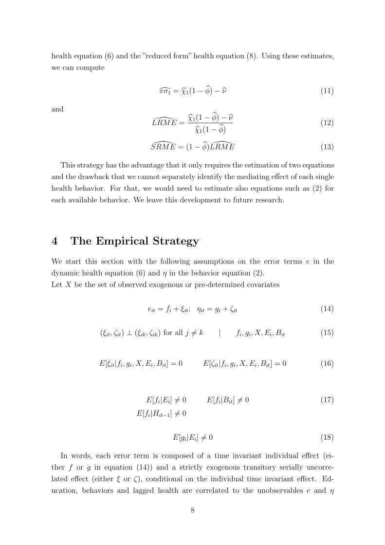
health equation (6) and the ”reduced form”health equation (8). Using these estimates,

we can compute

πσ1 = χ1(1− φ)− ν (11)

and

LRME =χ1(1− φ)− νχ1(1− φ)

(12)

SRME = (1− φ)LRME (13)

This strategy has the advantage that it only requires the estimation of two equations

and the drawback that we cannot separately identify the mediating effect of each single

health behavior. For that, we would need to estimate also equations such as (2) for

each available behavior. We leave this development to future research.

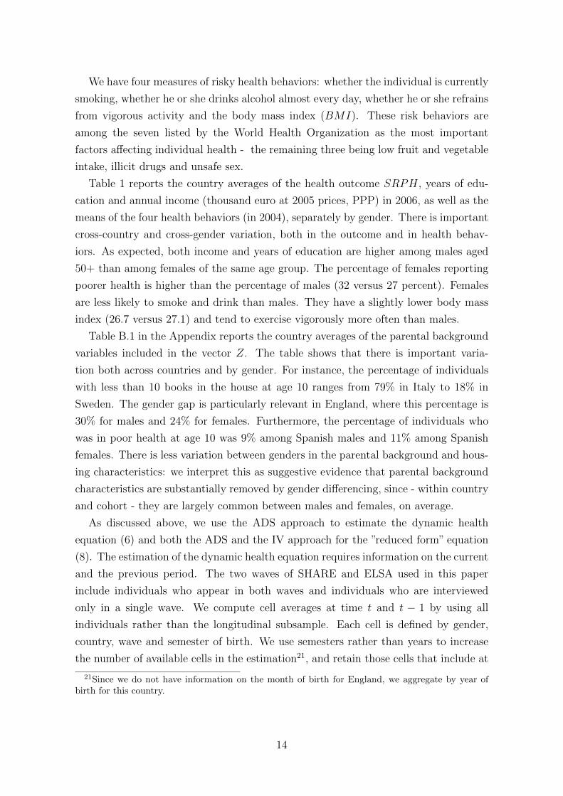
4 The Empirical Strategy

We start this section with the following assumptions on the error terms e in the

dynamic health equation (6) and η in the behavior equation (2).

Let X be the set of observed exogenous or pre-determined covariates

eit = fi + ξit; ηit = gi + ζit (14)

(ξit, ζit) ⊥ (ξik, ζik) for all j 6= k | fi, gi, X,Ei, Bit (15)

E[ξit|fi, gi, X,Ei, Bit] = 0 E[ζit|fi, gi, X,Ei, Bit] = 0 (16)

E[fi|Ei] 6= 0 E[fi|Bit] 6= 0 (17)

E[fi|Hit−1] 6= 0

E[gi|Ei] 6= 0 (18)

In words, each error term is composed of a time invariant individual effect (ei-

ther f or g in equation (14)) and a strictly exogenous transitory serially uncorre-

lated effect (either ξ or ζ), conditional on the individual time invariant effect. Ed-

ucation, behaviors and lagged health are correlated to the unobservables e and η

8

only via their correlations with the individual effects f and g, i.e. we do not as-

sume that these effects are independent of Ei, Bit, Hit−1. In our set-up, individ-

ual effects could be regarded as random without loss of generality given that we

are interested in partial regression coefficients holding these individual effects con-

stant. We regard (Hit, Ei, Bit, Hit−1, X, fi, gi) as a random sample from an artifi-

cial multivariate population with joint distribution p(Hit, Ei, Bit, Hit−1, X, fi, gi) =

p(Hit|Ei, Bit, Hit−1, X, fi, gi)p(Ei, Bit, Hit−1, X, fi, gi) and focus on the conditional dis-

tribution of Hit.

Since optimal education depends on the unobservables that affect preferences (η)

and the health production function (e) - see the illustrative example in the Appendix

- ordinary least squares estimates of the health production function fail to uncover

causal relationships. A similar problem affects the OLS estimates of the ”reduced

form” health function, because health in that equation depends both on education and

on the sequence of shocks affecting preferences and the health production function

(see equation (8)). An important drawback of the empirical studies investigating the

mediating effect of health behaviors on the education gradient is that they fail to

consider the endogeneity of education and behaviors (Lochner, 2011). In this paper,

we address these problems in an attempt to give a causal interpretation both to the

gradient and to the mediating role of behaviors.

In the past few years, several papers have estimated the causal effect of educa-

tion on health using the exogenous variation in educational attainment generated by

compulsory schooling laws. This instrumental variables (IV) approach can be used

to estimate the ”reduced form” health equation (8). In principle, the same approach

can also be applied to the dynamic health production function (6), provided that we

can find additional credible sources of exogenous variation which affect risky health

behaviors without influencing individual health (conditional on behaviors). This is a

very difficult task with the data at hand.9 Therefore, we turn to the identification

strategy suggested by Card and Rothstein (2007), which combines aggregation, selec-

tion on observables and fixed effects assumptions, to estimate both the dynamic health

production function and the ”reduced form” health equation. For the latter equation,

we compare the results obtained following the Card and Rothstein (2007) approach to

those obtained with the IV approach, using changes in compulsory education as the

relevant instrument. In the rest of this section, we illustrate the two approaches in

turn.

9Using instruments such as the price of alcohol or cigarettes does not work in our setup becausethese variables influence all cohorts in one country alike.

9

4.1 The Card-Rothstein approach

Consider the following empirical version of the dynamic health production function

Hicgbt = αg0 + αg1Bicgb(t−1) + αg2Eicgb + αg3Xicgb + αg4Hicgb(t−1) + ficgb + ξicgbt (19)

where X is a vector of controls, i denotes the individual, c the country, t calendar time,

g gender (M : males; F : females), b the birth cohort and we allow each explanatory

variable to have a gender-specific effect on health.

Following Card and Rothstein (2007), we can decompose the error term in equation

(19) as follows

ficgb + ξicgbt = fcgb + ξcgbt + εicgbt (20)

where fcgb + ξcgbt represents a common error component for individuals of the same

gender g and birth cohort b in country c at time t, and εicgbt is an individual-specific

idiosyncratic error component for which we assume

E[εicgbt|b, g, c, t] = 0 (21)

The individual-specific error term has mean zero across individuals of the same gender,

year of birth, country and time period.

We aggregate individual data into cells identified by country, time, birth cohort and

gender and define αs = αFs−αMs, with s = 0, .., 3. Taking gender differences for each

cell (∆ =females - males), we obtain

∆Hcbt = α0 + αM1∆Bcb(t−1) + α1BFcb(t−1) + αM2∆Ecb + α2E

Fcb + αM3∆Xcb + α3X

Fcb+

+αM4∆Hcbt−1 + α4HFcbt−1 + ∆fcb + ∆ξcbt (22)

where the superscript F refers to females. In this specification, αM1 and α1 + αM1

are the effects of health behaviors lagged once for males and females respectively.

Similarly, the gender gap in the ”returns” to education is given by coefficient α2.

Assumptions (14) to (18) guarantee that the vector [∆B,BF ,∆E,EF ,∆H−1, HF−1]

is orthogonal to ∆ξcbt.10 Differencing by gender eliminates all unobserved factors that

10To avoid confusion, we stress that ∆ξcbt is the difference between ξcbFt and ξcbMt, not the differ-ence between ξcbFt (ξcbMt) and ξcbFt−1 (ξcbMt−1), i.e. we are taking differences between genders in agiven calendar time not differences within gender over time.

10

are common to males and females for a given country c and birth cohort b, includ-

ing genetic and environmental effects, income components, medical inputs and the

organization of health care.11 Even after eliminating common unobservables, how-

ever, the residual error component ∆fcb could still be correlated with education and

lagged health behaviors. This could happen, for instance, if health conditions and

parental background during childhood differ systematically by gender or if labor mar-

ket discrimination affects individual income and access to health care, conditional on

educational attainment. To remove this correlation, we model this residual as

∆fcb = ψb + ψc + ψM1∆Zcb + ψ1ZFcb + ψM2∆Ycb + ψ2Y

Fcb + κcb (23)

where ψs = ψFs − ψMs, with s = 1, 2, ψb includes cohort dummies and country-

specific linear or quadratic trends in birth cohorts, ψc is a vector of country dummies,

Z a vector of observables, which includes a rich set of parental background character-

istics and health conditions during childhood12 and Y is real income. Our identifying

assumption is that, conditional on these variables which capture gender-specific ge-

netic and environmental effects, the error term κcb is orthogonal to levels and changes

in health behaviors and educational attainment.13

For the sake of brevity, we call this method ADS (aggregation cum differentiation

cum selection on observables). To illustrate, suppose that the key unobservable in

(19) is the latent time invariant (cell) average ability. The ADS method assumes that

part of this latent factor is common across genders and can be differenced out.14 The

residual gender-specific component is captured by cohort and country dummies as well

as by gender differences in parental background during childhood and initial health

conditions. Conditional on our identifying assumptions, equation (22) is estimated

by weighted least squares, using as weight(

1NM

+ 1NF

)−1

, where NM and NF are the

number of males and females in each cell, as suggested by Card and Rothstein (2007).

11See Zweifel and Breyer (1997).12There is a growing literature on the impact of childhood health on adult economic outcomes

(Banks et al. (2011) or Smith (2009)). The vector Z includes: childhood poor health, hospitalizationduring childhood, presence of serious diseases, had at most 10 books at home at age 10, mother andfather in the house at age 10, mother or father died during childhood, number of rooms in the houseat age 10, had hot water in the house at age 10, parents drunk or had mental problems at 10, hadserious diseases at age 15, born in the country.

13The inclusion of cohort and country dummies in (23) implies that cohort and country effectsdiffer by gender. In case of no gender differences in any of the above factors ∆fcb ≡ κcb.

14With respect to the standard fixed effect model set-up we are assuming that the conditionaldistribution of the individual fixed effect given (Ei, Bit, Hit−1, X) is common between genders. Otherthan this the conditional distribution is left unrestricted and the inference is conditional on this effect.

11

4.2 The IV approach

As an alternative approach, we also estimate the ”reduced form” health equation (8)

by instrumental variables, using as instrument for endogenous education the number

of years of compulsory education Y C. This is widely considered to be a credible

identification strategy, and one that has been extensively used in the literature (see

Lochner (2011) for a review). As in Brunello, Fort and Weber (2009), Brunello, Fabbri

and Fort (2009) and Fort et al. (2011), we apply this strategy to a multi-country setup

and exploit the fact that school reforms have occurred at different points in time in

several countries.

For each country and reform included in our sample, we construct pre-treatment and

post-treatment samples by identifying for each reform the pivotal birth cohort, defined

as the first cohort potentially affected by the change in mandatory school leaving age.

We include in the pre- and post-treatment samples all individuals born either before,

at the same time or after the pivotal cohort. By construction, the number of years

of compulsory education Y C “jumps” with the pivotal cohort and remains at the new

level in the post-treatment sample. The timing and intensity of these jumps varies

across countries, and we use the within country exogenous variation in the instrument

to identify the causal effects of schooling on health.

We include in equation (8) country fixed effects, cohort fixed effects and country-

specific linear or quadratic trends in birth cohorts. These trends account for country-

specific improvements in health that are independent of educational attainment.15 On

the other hand, country fixed effects control for national differences both in reporting

styles and in institutions affecting health. Notice that the older cohorts in our data are

healthier than average, having survived until relatively old age. Since the comparison

of positively selected pre-treatment individuals with younger post-treatment samples

is likely to result in a downward bias in the estimates, we control for this selection

process by including cohort fixed effects.

5 Data

The estimation of the ”reduced form” and the dynamic health equation requires data

on health outcomes, risky health behaviors, education, parental background and early

socio-economic and health conditions. The Survey of Health, Ageing and Retirement in

Europe (SHARE), the English Longitudinal Study of Ageing (ELSA) and their retro-

spective interviews satisfy these requirements. SHARE is a longitudinal dataset on the

15”Failure to account for secular improvements in health may incorrectly attribute those changes toschool reforms, biasing estimates toward finding health benefits of schooling.” (Lochner (2011), p.41)

12

health, socio-economic status and social relations of European individuals aged 50+,

and consists of two waves - 2004/5 and 2006/7 - plus a retrospective wave in 2008/9

(SHARELIFE), covering several European countries - Austria, Belgium, Switzerland,

Denmark, Spain, France, Germany, Italy, Greece, The Netherlands and Sweden.16

ELSA has similar characteristics and covers England.17 Since education is typically

accumulated in one’s teens or twenties, by focusing on individuals aged 50+ we are

considering the long-run effects of education on health.

The measure of health used in this paper is self-reported poor health (SRPH), a

dummy equal to 1 if the individual considers her health as fair or poor and to 0 if she

considers it as good, very good or excellent. This is a subjective and comprehensive

measure of health, which is conventionally used in the applied literature (Lochner,

2011). One may object that self-reported information is likely to be dominated by

noise and to fail to capture differences in more objective measures of health.18 This

is not the case here: among the individuals in the sample who reported poor health,

46% had hypertension, 69% had cardiovascular diseases and 79% suffered some long-

term illness. On average, they had 2.44 chronic diseases (certified by doctors). In

contrast, the percentage of individuals in good health with similar diseases was 28,

44 and 33 percent, respectively.19 Moreover, the latter group experienced only 1.10

chronic diseases. While our data contain information on chronic diseases, which can

be argued to be more objective than self-reported health, we have chosen to focus on

the latter in order to be able to compare our results with the bulk of estimates in the

relevant literature. However, we also present in the robustness section of this paper

estimates based on the number of chronic diseases.20

We measure educational attainment with years of education. The second wave of

SHARE provides information on the number of years spent in full time education. In

the first wave, however, participants were only asked about their educational quali-

fications. Thus, for the individuals participating only in the first wave, we calculate

their years of schooling using country-specific conversion tables. In ELSA, years of

education are computed as the difference between the age when full-time education

was completed and the age when education was started.

16The Czech Republic, Poland, Israel and Ireland joined in the second wave.17For England, we use waves 2 (2004/5) and 3 (2006/7).18For an early discussion about the importance of measurement error in self-reported health see

Bound (1991) and Butler et al. (1987) as well as Baker et al. (2004). These authors were primarilyconcerned with the impact of measurement error in equations determining the impact of healthon retirement and other labor market outcomes. Justification bias, i.e. non-working persons over-reporting specific conditions, is an obvious problem there.

19Heiss (2011) finds strong autocorrelation in self-reported health across waves and a strong corre-lation with future mortality for the Health and Retirement Study.

20Using the same dataset, we discuss at length how the education gradient varies with differentmeasures of health in a companion paper (Brunello et al., 2011).

13

We have four measures of risky health behaviors: whether the individual is currently

smoking, whether he or she drinks alcohol almost every day, whether he or she refrains

from vigorous activity and the body mass index (BMI). These risk behaviors are

among the seven listed by the World Health Organization as the most important

factors affecting individual health - the remaining three being low fruit and vegetable

intake, illicit drugs and unsafe sex.

Table 1 reports the country averages of the health outcome SRPH, years of edu-

cation and annual income (thousand euro at 2005 prices, PPP) in 2006, as well as the

means of the four health behaviors (in 2004), separately by gender. There is important

cross-country and cross-gender variation, both in the outcome and in health behav-

iors. As expected, both income and years of education are higher among males aged

50+ than among females of the same age group. The percentage of females reporting

poorer health is higher than the percentage of males (32 versus 27 percent). Females

are less likely to smoke and drink than males. They have a slightly lower body mass

index (26.7 versus 27.1) and tend to exercise vigorously more often than males.

Table B.1 in the Appendix reports the country averages of the parental background

variables included in the vector Z. The table shows that there is important varia-

tion both across countries and by gender. For instance, the percentage of individuals

with less than 10 books in the house at age 10 ranges from 79% in Italy to 18% in

Sweden. The gender gap is particularly relevant in England, where this percentage is

30% for males and 24% for females. Furthermore, the percentage of individuals who

was in poor health at age 10 was 9% among Spanish males and 11% among Spanish

females. There is less variation between genders in the parental background and hous-

ing characteristics: we interpret this as suggestive evidence that parental background

characteristics are substantially removed by gender differencing, since - within country

and cohort - they are largely common between males and females, on average.

As discussed above, we use the ADS approach to estimate the dynamic health

equation (6) and both the ADS and the IV approach for the ”reduced form” equation

(8). The estimation of the dynamic health equation requires information on the current

and the previous period. The two waves of SHARE and ELSA used in this paper

include individuals who appear in both waves and individuals who are interviewed

only in a single wave. We compute cell averages at time t and t − 1 by using all

individuals rather than the longitudinal subsample. Each cell is defined by gender,

country, wave and semester of birth. We use semesters rather than years to increase

the number of available cells in the estimation21, and retain those cells that include at

21Since we do not have information on the month of birth for England, we aggregate by year ofbirth for this country.

14

least two observations. We use data from 12 countries, all of which have participated

in at least two waves in the surveys.

We implement the IV approach by selecting 7 countries where the individuals in our

sample experienced at least one compulsory school reform: Austria, Denmark, Eng-

land, France, Italy, the Netherlands and the Czech Republic.22 A short description of

the compulsory school reforms used in this paper can be found in Appendix C. Since

the ”reduced form” equation (8) is static, we can use individuals who participated in

both waves and those who participated in either the first or the second wave. When

available, we measure the key variables (health, education) using the information pro-

vided by individuals during their second interview. For those who did not participate

to the second wave, we use the first wave.

6 Results

This section describes the results of our empirical analysis and is organized as follows:

first, the baseline estimates of the ADS model for the ”reduced form” and the dynamic

health equation are presented. Next, we discuss in Section 6.2 the reduced form esti-

mates based upon the IV approach. Finally, the ADS estimates of the ”reduced form”

health equation are compared to the IV results (Section 6.3). Section 6.4 concludes

with several robustness checks.

6.1 Baseline Estimates of the Reduced Form and Dynamic

Health Equations

As reviewed in Section 2, most of the earlier contributions to this literature fail to

consider the endogeneity of education and health behaviors in their health regressions.

For the sake of comparison with this literature, we start the illustration of our empirical

findings with the estimates of the ”reduced form” and dynamic health equations based

on micro data. We use a linear probability model, treat education and behaviors as

exogenous, and regress self-reported poor health on years of education and a vector

of variables, which varies according to whether we consider the ”reduced form” or the

dynamic health equation and we include parental and early life controls or not.

For each regression, we pool males and females but allow for the full set of interac-

tions of each explanatory variable with a gender dummy. Preliminary testing suggests

22The inclusion of the last country is possible because the estimation of the ”reduced form” healthequation does not require two waves per country. We exclude Germany and Sweden because schoolreforms in these countries were implemented at the regional level and our information on the regionwhere the individuals completed their education is not accurate.

15

that we cannot reject the null hypothesis that cohort, country, time and early life

effects do not vary by gender.23 We therefore report only those parsimonious results.

Table (2) is organized in two columns, one for the ”reduced form” and the other for

the dynamic health equation, which includes health behaviors lagged once, the first

lag of health and current income.

In the ”reduced form”equation the marginal effect of one additional year of schooling

on poor health is equal to −0.012 for males and to −0.017 for females, a relatively

small effect when compared to the existing literature for Europe, which points to an

effect in the range −0.026 to −0.081 (Lochner (2011), Table 6). This difference can be

explained, at least in part, if the education gradient declines with age, given that our

sample consists of individuals aged 50+ and the samples used in the literature typically

include also younger individuals. Coefficients of parental and early life conditions,

including poor health at age 10, are statistically significant and point in the expected

direction: poor health conditions at 10 or 15 as well as poor parental environments at

early ages increase self-perceived poor health at age 50+. Importantly, the inclusion

of these variables reduces the gradient by 15 to 20 percent with respect to a more

parsimonious specification without those (not shown in the table), which suggests that

they capture at least in part the positive correlation between educational attainment

and unobserved individual effects such as ability and initial health.

Turning to the dynamic health equation with early life variables, we find that our

measures of risky health behaviors have statistically significant coefficients, with pre-

dictable correlations: smoking, refraining from vigorous activity and poor diet leading

to higher BMI are positively related to self-perceived poor health. Somewhat unexpect-

edly, however, drinking alcohol almost every day is negatively related to self-reported

poor health. Annual real income is negatively associated to perceived poor health,

which exhibits important persistence over time - the lagged dependent variable has a

coefficient close to 0.5 but is statistically distinct from 1.

Adding health behaviors, income and lagged health reduces the coefficient of ed-

ucation from −0.012 to −0.005 for males, and from −0.017 to −0.006 for females.

Assuming that the returns to education for the sample of countries under study is

equal to 0.0724, the estimated mediating effect of behaviors lagged once is 9.7% for

males and 16.8% for females - see Table 3. In the long run, when we include the effect

of earlier health behaviors, the mediating effect almost doubles to 18.9% for males and

23The joint hypothesis is not rejected at the 5 percent level of confidence (p-value: 0.094). We testedseparately also the null that the following effects are common between genders: cohort effect (p-value:0.894), country effect (p-value: 0.42), background variables (p-value: 0.263), trends (p-value: 0.112)and we never reject the null at conventional significance levels.

24See for instance the estimates in Brunello, Fort and Weber (2009). Adding income to equation(6) implies that LRME is equal to πσ1

(πσ1+ν+qρY ), where q is the coefficient of income in the dynamic

health equation, ρ is the estimated return to education and Y is average income.

16

32.3% for females, suggesting that considering only their first lag may substantially

underestimate the contribution of health behaviors to the education gradient. Our

estimated long-run effects are smaller than those found by Cutler et al. (2008), who

use a different approach but conclude that measured health behaviors account for over

40% of the education gradient (on mortality) in a sample of non-elderly Americans.25

Although the inclusion of parental and early life controls in our regression is likely

to attenuate the correlation between education, health behaviors and unobservables,

there is no guarantee that this correlation will disappear entirely. In order to identify

the causal impact of education on health and behaviors, we apply the ADS procedure

discussed in Section 4.1, which combines aggregation and gender differentiation with

selection on observables. The specification tests carried out on the micro data suggest

that cohort, country and early life effects do not differ significantly by gender. As a

consequence, when we take gender differences of cell data, these common effects are

removed together with common unobservables. Therefore, our preferred specification

of the ADS model includes only differences in early life variables and excludes common

country and cohort dummies and common trends in birth cohorts.26

Our results for the ADS model are shown on the right-hand side of Table 2, both

for the ”reduced form” and for the dynamic health equation. When we consider the

former, we find that the overall effect of education on poor health is negative and larger

in absolute values for females (−0.026) than for males (−0.010). Parental and early

life variables are jointly statistically significant (p-value: 0.009), mainly because of the

gender differences in poor health at age 10. Turning to the dynamic health equation, we

find that the effect of education conditional on behaviors is much smaller (−0.015 for

females and −0.003 for males) than in the ”reduced form”. While the precision of the

estimates of the effects of behaviors declines in the cell data with respect to the micro

data, we cannot reject the null hypothesis that these effects are jointly statistically

significant. Finally, income effects are insignificant and the persistence of self-reported

poor health over time is substantially reduced with respect to the estimates based on

micro data.

Aggregation and differentiation increases the absolute value of the overall education

gradient for females from 0.017 to 0.026 but has limited effects on the gradient for

males, which marginally declines in absolute value from 0.012 to 0.010. The short-run

and the long-run mediating effects of health behaviors are also affected. As shown in

Table 3, when compared to the estimates based on micro data, the long-run mediating

effect for males declines in absolute value (from 0.007 to 0.004) but increases as a

25These authors estimate a static health equation, which includes income and occupation amongthe explanatory variables, and use the following measures of health behaviors: current smoker, eversmoker, number of cigarettes per day, obesity, regular exercise and use of seat belts always.

26This is equivalent to assuming ψb = 0, ψc = 0 and ψ1 = 0 in equation (23).

17

share of the gradient (from 18.9 to 44.5%). The opposite happens for females, for

whom this effect increases in absolute value from 0.005 to 0.006 but declines as share

of the gradient (from 32.3% to 22.8%).

In sum, when we explicitly take into account the endogeneity of education and health

behaviors, we find that the long-run mediating effect of the latter ranges between 23

and 45% of the total education gradient. While the effect of education on behaviors

accounts for an important share of the gradient, much remains to be explained, either

by the role played by unmeasured behaviors or by effects that do not involve behaviors,

such as better decision making, stress reduction and more health-conscious peers.

6.2 IV Estimates of the Reduced Form Health Equation

In this section, we present the estimates of the ”reduced form”health equation obtained

using instrumental variables. We instrument education with the number of years of

compulsory education, which varies across countries and cohorts because of compulsory

schooling reforms. For each country, we construct a sample of treated individuals, who

have experienced a change in compulsory education, and a control sample, with no

change in compulsory schooling. Since our data include only individuals aged 50+, we

need to focus on school reforms which took place between the 1940s and the 1960s,

and to restrict our attention to a sub-sample of 7 countries affected by these reforms.

Table 4 shows the selected countries, the years and the content of the reforms as well

as the pivotal cohorts, i.e. the first cohorts potentially affected by the reforms (see

Appendix C for a short description of the education reforms used in this paper).

In order to ensure that individuals spent their schooling in their host country, we

restrict our sample to individuals, who participated in the first or second wave of

SHARE (second or third wave in ELSA), and were born in the country or migrated

there before age 5. Additionally, we control for country fixed effects, cohort fixed effects

as well as for some individual characteristics (whether the individual is foreign-born,

whether there was a proxy respondent for the interview and indicators for the interview

year). We capture smooth trends in education and health by adding country-specific

polynomials in cohorts. In particular, we estimate two specifications, one with a linear

trend and one with a quadratic trend.

Since the key identifying assumption that changes in average education within coun-

try can be fully attributed to the reforms is more plausible when the window around

the pivotal cohort is small, we estimate our model using two alternative samples, one

including individuals who were born up to 10 years before and after the reforms and

another where the relevant window is +7,-7. The two samples consist of 15,960 and

18

12,294 individuals respectively. Table 5 shows summary statistics by country for the

larger sample.

Table 6 presents our estimates of the health-education gradient for both males and

females. We report the OLS, 2SLS, ITT (Intention-To-Treat), first stage and IV-Probit

estimates for both samples, using two alternative specifications for the country-specific

trends (linear or quadratic). The OLS estimate of the gradient is equal to −0.017 for

males and to −0.024 or −0.025 for females, depending on the selected window. The

estimated magnitude of the gradient increases with instrumental variables: we find

that one additional year of schooling decreases the probability of poor health by 4− 9

percentage points for females and by 5− 6 percentage points for males, depending on

the selected window. IV-Probit estimations yield very similar results. The IV strategy

works well: our first stage regressions show that the instrument is relevant and not weak

(F-Statistics between 13 and 41) and that one additional year of compulsory schooling

increases actual schooling by a quarter to a third of a year, broadly in line with previous

findings in the literature using similar identification strategies. We interpret the IV

estimates as Local Average Treatment Effects, i.e. the effects of schooling on health

for the individuals affected by the reforms. These individuals typically belong to the

lower portion of the distribution of education.

6.3 IV and ADS Results Compared

Next, we compare the education gradients estimated with the IV and the ADS ap-

proaches (Table 7). For the IV approach, we report the estimates with the linear

trend specification and the largest window (±10). We find that education reduces

self-perceived poor health by 4 and 4.8 percentage points for females and males re-

spectively. The ADS approach yields smaller estimates - in absolute value - for females

(2.6 percentage points) and especially for males (1 percentage point).

Since the two approaches are based on a different set of countries and cohorts, we

re-estimate the ADS model for the same sample used in the IV approach. The results

are shown in the last column of Table 7. The magnitudes of the ADS estimates in this

new sample increase somewhat, to 2.8 percentage points for females and to 2 for males,

but remain smaller in absolute value than the IV estimates. To explain this difference,

we notice that, while IV estimates are Local Average Treatment Effects, i.e. the causal

effects of education on health for the individuals affected by the compulsory schooling

reforms, the estimates obtained with the ADS approach pertain to a randomly drawn

individual from the entire sample. If the protective effect of education on health is more

pronounced for persons with lower education, this could explain the higher magnitudes

obtained with the IV approach.

19

6.4 Robustness Checks

In this section, we focus on the ADS approach and consider several robustness checks.

We start by collapsing data by gender, country and year rather than semester of birth.

By doing so, we reduce the sample size by almost a half. As shown in the first two

columns of Table 8, the effect of education on health is virtually unaffected for females

but declines for males. Next, we omit England to take into account that English data

are drawn from a different (although quite similar) survey and can only be collapsed

by year of birth. The next two columns of Table 8 show that the education gradient

changes only marginally. However, when we decompose the gradient into the effect

mediated by behaviors and the residual effect, we find that the LRME in this sub-

sample is smaller than in the full sample, and is equal to 8.5% and 11.1% of the

gradient for females and males respectively.27

Furthermore, we notice that the older cohorts in our data are strongly selected

by mortality patterns.28 To control for this, we add to the regressions the level and

the gender difference of life expectancy at birth, which vary by country, gender and

birth cohort. Since these data are not available for Greece29, we are forced to omit

this country from the sample. As displayed by the last two columns in the table,

life expectancy is never statistically significant in the ”reduced form” health equation,

and only marginally significant (at the 10% level of confidence) in the dynamic health

equation. We conclude that adding this variable does little to our empirical estimates.

We also run our estimates for the sub-sample of individuals aged 50 to 69 and find

that one additional year of schooling reduces self-reported poor health by 11.5% for

males and by 22.4% for females. These percentages are closer to those found in the

literature. Since survivors aged 70 to 86 might be better educated and might experience

a stronger protective role of education on health than the average individual in the

same age group - i.e. they might have a higher education gradient - it is unlikely that

the decline of the gradient with age is driven by selection effects.

One may think of several factors affecting changes in the education gradient by age

group. On the one hand, the gradient could decline among older individuals because

cognitive abilities decline with age. On the other hand, the effect of behaviors on

health accumulates over time, which should increase the gradient with age. At the

27We have also estimated our equations on two sub-samples of countries, based on their proximityto the Mediterranean Sea, but cannot reject the hypothesis that the estimated coefficients are notstatistically different.

28Age in our sample ranges from 50 to 86.29We use data on life expectancy at birth from the Human Mortality & Human Life-Table

Databases. The databases are provided by the Max Planck Institute for Demographic Research(www.demogr.mpg.de). The data are missing for some cohorts and for Greece. We use period mea-sures of life expectancy at birth since cohort measures are not available for all the cohorts consideredin the study.

20

same time, one may speculate that differences by education increase with age because

the older care more about their health. While these factors go in different directions,

our empirical results suggest that their balance is tilted in favor of the first.

Finally, we consider an alternative and more objective measure of health outcome,

the number of chronic diseases. While this number is reported by interviewed indi-

viduals, it is conditional on screening, i.e. each condition must have been detected

by a doctor. Table 9 presents both the ADS estimates of the ”reduced form” and

the dynamic health equation, and the IV estimates of the ”reduced form”. Using the

ADS method, we find evidence of a negative and statistically significant gradient for

females (−0.057) and of a positive, small and imprecisely estimated gradient for males

(0.012). The directions of these effects are confirmed but their magnitudes in abso-

lute values are larger (−0.157 for females and 0.080 for males) when we apply the IV

method. Defining P (D) as the probability of reporting a condition, this probability

is the product of the probability of undergoing screening P (S) and the probability of

having a condition conditional on screening, P (D|S). We speculate that in the case of

males the positive effect of education on the number of diseases may be driven by the

fact that better educated males choose more intensive screening.

Turning to the decomposition of the gradient into the mediating effect of behaviors

and the residual effect, we find that SRME and LRME for females are equal to 16.5

and 28.1 percent respectively, not far from the effects estimated for self-reported poor

health. In the case of males, the estimated parameters do not meet the conditions for

both SRME and LRME to be well defined within the range [0, 1].

7 Conclusions

In this paper we have studied the contribution of health behaviors to the education

gradient by distinguishing between short-run and long-run mediating effects: while in

the former only current or lagged behaviors are taken into account, in the latter we

consider the entire history of behaviors. We have proposed a strategy to estimate and

decompose the education gradient which takes into account both the endogeneity of

educational attainment as well as the endogenous choice of health behaviors.

Our results show that one additional year of schooling reduces self-reported poor

health by 7.1% for females and by 3.1% for males. Health behaviors - measured by

smoking, drinking, exercising and the body mass index - contribute to this gradient.

We find that the mediating effect of behaviors accounts for 23% to 45% of the entire

effect of education on health, depending on gender. This contribution is reduced if we

only consider current behaviors or behaviors in the immediate past, as usually done in

21

the empirical literature. Using a completely different strategy - instrumental variables

estimation - we find corroborating results for the education gradient.

Since the gradient is key to understanding inequality in health and life expectancy

and is also used to assess overall returns to education (Lochner, 2011), it is important

to understand the mechanisms governing it. Many of the discussed health behaviors

are individual consumption decisions, changes thereof come at personal costs, e.g.

abstaining from smoking or drinking good wine. Increases in health achieved by such

costly changes in behavior have, thus, to be distinguished from changes resulting from

the free benefits of education, such as lower stress or better decision making. This

distinction is relevant for political decisions about subsidizing schooling. If individuals

are aware of the health-fostering effects of schooling and these are private, then there

is no room for public policy. If individuals are unaware of these benefits, the case for

public policy is stronger if the health benefits of schooling are primarily free rather than

being based on the costly health behavior decisions of individuals (Lochner, 2011).

22

8 Tables

23

Table 1: Descriptive statistics, baseline estimation sample (micro data), males (M)and females (F).

Country Self-rep poor health Education Income Age ObsM F M F M F M F M F

Austria 0.27 0.31 11.04 9.47 18.74 10.74 65.14 66.18 260 364Belgium 0.24 0.29 12.36 11.55 16.09 10.82 65.24 65.59 905 1044Denmark 0.21 0.26 11.25 10.98 16.34 13.02 64.57 65.68 385 399England 0.28 0.29 11.26 11.20 20.67 14.25 67.50 67.35 1673 2050France 0.32 0.38 12.17 11.29 23.53 14.04 65.36 66.35 486 638Germany 0.29 0.35 13.58 12.23 24.50 8.57 65.23 63.69 310 342Greece 0.19 0.25 9.49 8.16 14.95 6.90 65.10 64.78 717 801Italy 0.38 0.50 8.08 7.11 13.07 6.55 66.42 65.16 602 722Netherlands 0.26 0.29 11.88 11.23 22.92 11.29 65.33 64.66 526 599Spain 0.39 0.52 7.99 7.50 13.65 5.52 67.30 66.44 364 458Sweden 0.22 0.26 11.42 11.61 16.81 13.00 65.94 65.38 512 615Switzerland 0.12 0.18 12.25 10.68 29.89 14.10 66.01 64.85 197 232All 0.27 0.32 11.02 10.37 18.66 11.17 66.03 65.86 6937 8264

Country Smoking−1 Drinking−1 No vigorous exercise−1 BMI−1

M F M F M F M FAustria 0.21 0.05 0.17 0.17 0.64 0.73 27.46 26.94Belgium 0.37 0.20 0.20 0.12 0.61 0.75 26.95 26.06Denmark 0.37 0.20 0.31 0.28 0.48 0.52 26.49 25.57England 0.22 0.14 0.13 0.12 0.75 0.81 27.81 28.15France 0.52 0.24 0.19 0.09 0.59 0.73 26.57 25.74Germany 0.26 0.11 0.21 0.14 0.44 0.43 26.83 26.04Greece 0.18 0.03 0.36 0.20 0.60 0.67 27.11 26.73Italy 0.60 0.29 0.25 0.14 0.65 0.74 27.11 26.56Netherlands 0.38 0.28 0.24 0.24 0.52 0.54 26.26 26.17Spain 0.45 0.11 0.29 0.10 0.63 0.74 27.62 27.98Sweden 0.10 0.03 0.12 0.20 0.48 0.60 26.55 25.53Switzerland 0.34 0.19 0.24 0.19 0.48 0.57 25.78 24.76All 0.32 0.16 0.21 0.15 0.61 0.70 27.07 26.72

Notes: The upper panel refers to the second wave of SHARE/third wave of ELSA in 2006/07 andthe lower panel refers to the first wave in SHARE/second wave in ELSA in 2004/05.

24

Table 2: Baseline Results - Micro and ADS Model

Micro-estimates ADS-modelReduced form Dynamic HE Reduced form Dynamic HE

Femaleseducation -0.017 -0.006 -0.026 -0.015

(0.001)*** (0.001)*** (0.005)*** (0.005)***self-rep poor healtht−1 0.479 0.246

(0.012)*** (0.046)***drinkingt−1 -0.025 -0.013

(0.012)** (0.053)smokingt−1 0.052 -0.034

(0.012)*** (0.056)No vigorous 0.032 0.040exerciset−1 (0.009)*** (0.042)BMIt−1 0.007 0.003

(0.001)*** (0.004)incomet -0.000 -0.002

(0.000)** (0.001)Maleseducation -0.012 -0.005 -0.010 -0.003

(0.001)*** (0.001)*** (0.005)* (0.005)self-rep poor healtht−1 0.486 0.308

(0.014)*** (0.046)***drinkingt−1 -0.041 -0.062

(0.010)*** (0.038)smokingt−1 0.030 0.043

(0.011)*** (0.042)No vigorous 0.049 0.089exerciset−1 (0.009)*** (0.041)**BMIt−1 0.006 0.011

(0.001)*** (0.005)**incomet -0.000 -0.001

(0.000)** (0.001)Early lifefew books in HH 0.043 0.022 0.053 0.040

(0.009)*** (0.008)*** (0.035) (0.033)serious diseases at 15 0.017 0.004 0.028 0.004

(0.008)** (0.007) (0.036) (0.035)poor health at 10 0.117 0.062 0.158 0.135

(0.014)*** (0.012)*** (0.052)*** (0.049)***hospital at 10 0.032 0.025 0.004 0.042

(0.016)** (0.014)* (0.063) (0.061)Principal components

parents drunk or had 0.036 0.018 0.011 0.025mental problems at 10 (0.009)*** (0.008)** (0.039) (0.038)parental absence at 10 0.011 0.007 -0.008 -0.009

(0.011) (0.009) (0.039) (0.037)poor housing at 10 0.016 0.013 0.023 0.014

(0.004)*** (0.004)*** (0.017) (0.016)Observations 15,201 15,201 736 734

Notes: Cohort fixed effects and country-specific quadratic trends in cohorts are included in the firsttwo columns. ***, ** and * indicate statistical significance at the 1-percent, 5-percent and 10-percentlevel.

25

Table 3: Decomposition - Micro and ADS Model

Females MalesMicro-model ADS-model Micro-model ADS-model

Health-Education Gradient (HEG) -0.017 -0.026 -0.012 -0.010- behaviors (short-term) -0.003 -0.004 -0.004 -0.003- behaviors (long-term) -0.005 -0.006 -0.007 -0.004- residual (direct effect) -0.012 -0.020 -0.010 -0.006Mediating effect as fraction of HEG- SRME (short-term) 0.168 0.172 0.097 0.308- LRME (long-term) 0.323 0.228 0.189 0.445

Notes: Computations based on the estimates reported in Table 2.

Table 4: Compulsory schooling reforms in Europe

Country Reform Years of Compulsory Education Pivotal Cohort

Austria 1962/66 8 to 9 1951Czech Republic 1948 8 to 9 1934

1953 9 to 8 19391960 8 to 9 1947

Denmark 1958 4 to 7 1947England 1947 9 to 10 1933France 1959/67 8 to 10 1953Italy 1963 5 to 8 1949Netherlands 1942 7 to 8 1929

1947 8 to 7 19331950 7 to 9 1936

Table 5: Summary Statistics IV - Sample 10

Country Self-rep poor health Education Compulsory Edu Age Obs

Austria 0.233 11.363 8.237 58.971 782Czech Republic 0.418 12.026 8.535 63.304 2,452Denmark 0.208 11.802 5.642 59.194 1,898England 0.373 10.713 9.585 72.355 4,672France 0.331 11.324 8.275 63.668 2,223Italy 0.337 8.822 6.032 59.631 2,093Netherlands 0.338 10.613 8.263 69.95 1,840

All 0.339 10.901 8.088 65.588 15,960

26

Table 6: Health-Education Gradient - IV approach

Sample 10 Sample 7lin-trend qu-trend lin-trend qu-trend

FemalesOLS -0.024 -0.024 -0.025 -0.025

(0.002)*** (0.002)*** (0.002)*** (0.002)***2SLS -0.040 -0.064 -0.041 -0.085

(0.024)* (0.034)* (0.035) (0.032)***ITT -0.014 -0.017 -0.011 -0.023

(0.008)* (0.008)** (0.009) (0.008)***First Stage 0.344 0.253 0.263 0.271

(0.053)*** (0.058)*** (0.053)*** (0.058)***IV-Probit -0.042 -0.057 -0.041 -0.073

(0.022)* (0.025)** (0.032) (0.017)***F-Stat (First Stage) 41.93 18.95 24.89 21.66Observations 8,602 8,602 6,631 6,631

MalesOLS -0.017 -0.017 -0.017 -0.017

(0.002)*** (0.002)*** (0.002)*** (0.002)***2SLS -0.048 -0.054 -0.062 -0.064

(0.029)* (0.029)* (0.029)** (0.034)*ITT -0.016 -0.018 -0.020 -0.020

(0.009)* (0.008)** (0.008)** (0.010)**First Stage 0.323 0.318 0.313 0.298

(0.076)*** (0.078)*** (0.079)*** (0.082)***IV-Probit -0.047 -0.051 -0.056 -0.057

(0.024)** (0.022)** (0.019)*** (0.022)***F-Stat (First Stage) 17.87 16.62 15.66 13.07Observations 7,358 7,358 5,663 5,663

Notes: ***, ** and * indicate statistical significance at the 1-percent, 5-percent and 10-percent level.

Table 7: Health-Education Gradient - IV and ADS compared

ADS-modelIV-estimate All countries IV-sample

Females -0.040 -0.026 -0.028(0.024)* (0.005)*** (0.007)***

Males -0.048 -0.010 -0.020(0.029)* (0.005)* (0.008)**

Notes: ***, ** and * indicate statistical significance at the 1-percent, 5-percent and10-percent level.

27

Table 8: Robustness - ADS Model

ADS year panel ADS w/o ENG ADS l-exp, w/o GRCRed form Dynamic HE Red form Dynamic HE Red form Dynamic HE

Femaleseducation -0.025 -0.011 -0.023 -0.016 -0.03 -0.018

(0.006)*** (0.007) (0.005)*** (0.006)*** (0.006)*** (0.006)***self-rep poor healtht−1 0.307 0.240 0.252

(0.063)*** (0.046)*** (0.052)***drinkingt−1 0.017 -0.017 -0.031

(0.069) (0.052) (0.056)smokingt−1 -0.080 -0.043 -0.031

(0.076) (0.056) (0.063)No vigorous -0.016 0.021 0.036exerciset−1 (0.057) (0.044) (0.045)BMIt−1 0.001 0.000 0.002

(0.005) (0.005) (0.004)incomet -0.001 -0.003 -0.003

(0.002) (0.002)* (0.002)*Maleseducation -0.006 0.004 -0.008 -0.004 -0.010 -0.004

(0.007) (0.007) (0.005) (0.005) (0.006)* (0.006)self-rep poor healtht−1 0.301 0.319 0.295

(0.060)*** (0.046)*** (0.051)***drinkingt−1 -0.011 0.078 -0.067

(0.051) (0.038)** (0.042)smokingt−1 0.001 -0.038 0.038

(0.056) (0.042) (0.049)No vigorous 0.076 0.090 0.077exerciset−1 (0.054) (0.043)** (0.044)*BMIt−1 0.005 0.014 0.011

(0.007) (0.006)** (0.006)**incomet -0.002 -0.001 -0.001

(0.001) (0.001) (0.001)Early lifefew books in HH 0.024 -0.006 0.050 0.051 0.085 0.076

(0.048) (0.047) (0.035) (0.034) (0.038)** (0.036)**serious diseases at 15 0.110 0.070 0.021 0.007 0.021 -0.006

(0.051)** (0.050) (0.037) (0.035) (0.038) (0.037)poor health at 10 0.185 0.170 0.137 0.109 0.164 0.146

(0.073)** (0.070)** (0.053)*** (0.050)** (0.053)*** (0.051)***hospital at 10 -0.078 -0.028 0.060 0.097 -0.009 0.016

(0.093) (0.091) (0.065) (0.062) (0.065) (0.062)Principal components

parents drunk or had -0.015 0.010 0.029 0.043 -0.009 0.011mental problems at 10 (0.054) (0.053) (0.041) (0.039) (0.041) (0.040)parental absence at 10 0.047 0.029 -0.022 -0.016 0.009 0.005

(0.056) (0.054) (0.040) (0.038) (0.041) (0.039)poor housing at 10 0.039 0.029 0.022 0.010 0.014 0.004

(0.023)* (0.022) (0.017) (0.016) (0.018) (0.018)Life-expectancyfemales 0.007 0.009

(0.005) (0.005)*males 0.005 0.007

(0.003) (0.004)*Observations 389 387 701 701 640 638

Notes: ***, ** and * indicate statistical significance at the 1-percent, 5-percent and 10-percent level.

28

Table 9: Number of chronic diseases - ADS and IV Model

ADS-Model IV (Sample 10, lin-trend)Reduced form Dynamic HE Reduced form

Femaleseducation -0.057 -0.024 -0.157

(0.015)*** (0.016) (0.091)*# chronic diseasest−1 0.413

(0.044)***drinkingt−1 -0.044

(0.161)smokingt−1 0.007

(0.178)No vigorous 0.279exerciset−1 (0.131)***BMIt−1 0.012

(0.305)incomet -0.002

(0.004)Maleseducation 0.012 -0.006 0.080

(0.017) (0.016) (0.066)# chronic diseasest−1 0.337

(0.046)***drinkingt−1 -0.089

(0.116)smokingt−1 0.045

(0.147)No vigorous 0.220exerciset−1 (0.198)BMIt−1 0.041

(0.016)*incomet -0.004

(0.005)Early lifefew books in HH -0.135 -0.133

(0.110) (0.102)serious diseases at 15 0.067 0.084

(0.114) (0.106)poor health at 10 0.084 -0.004

(0.164) (0.151)hospital at 10 0.081 0.112

(0.200) (0.186)Principal components

parents drunk or had 0.149 0.124mental problems at 10 (0.124) (0.117)parental absence at 10 -0.128 -0.112

(0.123) (0.114)poor housing at 10 0.069 0.037

(0.054) (0.050)Observations 736 734 8,602 females, 7,358 males

Notes: ***, ** and * indicate statistical significance at the 1-percent, 5-percent and 10-percentlevel.

29

References

Adams, Scott J. (2002), ‘Educational attainment and health: Evidence from a sample

of older adults’, Education Economics 10(1), 97–109.

Albouy, Valerie and Laurent Lequien (2009), ‘Does compulsory education lower mor-

tality?’, Journal of Health Economics 28(1), 155–168.

Arendt, Jacob Nielsen (2005), ‘Does education cause better health? A panel data

analysis using school reforms for identification’, Economics of Education Review

24(2), 149–160.

Arendt, Jacob Nielsen (2008), ‘In sickness and in health - till education do us part:

Education effects on hospitalization’, Economics of Education Review 27(2), 161–

172.

Baker, Michael, Mark Stabile and Catherine Deri (2004), ‘What do self-reported, ob-

jective, measures of health measure?’, Journal of Human Resources 39(4), 1067–

1093.

Banks, James, Zoe Oldfield and James P. Smith (2011), Childhood health and differ-

ences in late-life helath outcomes between England and the United States, Working

Paper 17096, National Bureau of Economic Research (NBER).

Bound, John (1991), ‘Self-reported versus objective measures of health in retirement

models’, Journal of Human Resources 26(1), 106–138.

Braakmann, Nils (2011), ‘The causal relationship between education, health and health

related behaviour: Evidence from a natural experiment in England’, Journal of

Health Economics 30, 753–763.

Brunello, Giorgio, Daniele Fabbri and Margherita Fort (2009), Years of schooling,

human capital and the body mass index of European females, IZA Discussion Paper

4667, Institute for the Study of Labor (IZA).

Brunello, Giorgio, Margherita Fort and Guglielmo Weber (2009), ‘Changes in com-

pulsory schooling, education and the distribution of wages in Europe’, Economic

Journal 119(March), 516–539.

Brunello, Giorgio, Margherita Fort, Nicole Schneeweis and Rudolf Winter-Ebmer

(2011), The causal effect of education on health: Evidence from older Europeans.

mimeo, University of Linz, Austria.

30

Butler, J. S., Richard V. Burkhauser, Jean M. Mitchell and Theodore P. Pincus (1987),

‘Measurement error in self-reported health variables’, The Review of Economics and

Statistics 69(4), 644–650.

Card, David. and Jesse Rothstein (2007), ‘Racial segregation and the black-white test

score gap’, Journal of Public Economics 91, 2158–2184.

Cawley, John and Christopher Ruhm (2011), The economics of risky health behaviors,

Working Paper 17081, National Bureau of Economic Research (NBER).

Clark, Damon and Heather Royer (2010), The effect of education on adult health

and mortality: Evidence from Britain, Working Paper 16013, National Bureau of

Economic Research (NBER).

Conti, Gabriella, James J. Heckman and Sergio Urzua (2010), ‘The education-health

gradient’, American Economic Review: Papers and Proceedings 100, 234–238.

Contoyannis, Paul and Andrew Michael Jones (2004), ‘Socio-economic status, health

and lifestyle’, Journal of Health Economics 23, 965–995.

Cutler, David M. and Adriana Lleras-Muney (2006), Education and health: Evalu-

ating theories and evidence, Working Paper 12352, National Bureau of Economic

Research.

Cutler, David M. and Adriana Lleras-Muney (2010), ‘Understanding differences in

health behaviour by education’, Journal of Health Economics 29, 1–28.

Cutler, David M., Adriana Lleras-Muney and Tom Vogl (2008), Socioeconomic status

and health: Dimensions and mechanisms, Working Paper 14333, National Bureau

of Economic Research.

Cutler, David M., Edward L. Glaeser and Jesse M. Shapiro (2003), ‘Why have Amer-

icans become more obese?’, Journal of Economic Perspectives 17(3), 93–118.

Feinstein, Leon, Ricardo Sabates, Tashweka Anderson, Annik Sorhaindo and Cathie

Hammond (2006), Measuring the Effects of Education on Health and Civic En-

gagement: Proceedings of the Copenhagen Symposium, Paris, chapter What are the

effects of education on health?, pp. 171–354.

Fort, Margherita (2006), ‘Education reforms across Europe: A toolbox for empirical

research’. Paper version: May 11, 2006, mimeo.

31

Fort, Margherita, Nicole Schneeweis and Rudolf Winter-Ebmer (2011), More schooling,

more children: Compulsory schooling reforms and fertility in Europe, Working Paper

1105, Department of Economics, Johannes Kepler University of Linz.

Garrouste, Christelle (2010), 100 years of educational reforms in Europe: A contextual

database, European Commission Joint Research Center, Luxembourg: Publications

Office of the European Union.

Grossman, Michael (1972), ‘On the concept of health capital and the demand for

health’, Journal of Political Economy 80, 223–255.

Heiss, Florian (2011), ‘Dynamics of self-rated health and selective mortality’, Empirical

Economics 40, 119–140.

Juerges, Hendrik, Eberhard Kruk and Steffen Reinhold (2009), The effect of compul-

sory schooling on health: Evidence from biomarkers, Discussion Paper 183–2009,

Mannheim Institute for the Economcis of Aging (MEA).

Kempter, Daniel, Hendrik Juerges and Steffen Reinhold (2011), ‘Changes in compul-

sory schooling and the causal effect of education on health: Evidence from Germany’,

Journal of Health Economics 30(2), 340–354.

Levin, Jesse and Erik J. S. Plug (1999), ‘Instrumenting education and the returns to

schooling in the Netherlands’, Labour Economics 6, 521–534.

Lochner, Lance (2011), Non-production benefits of education: Crime, health, and good

citizenship, Working Paper 16722, National Bureau of Economic Research (NBER).

Mazumder, Bhashkar (2008), ‘Does education improve health: A reexamination of the

evidence from compulsory schooling laws’, Economic Perspectives 33(2), 1–15.

Meghir, Costas, Marten Palme and Emilia Simeonova (2011), Education, health and

mortality: Evidence from a social experiment. mimeo, Stockholm University.

Oreopoulos, Phillip (2007), ‘Do dropouts drop out too soon? Wealth, health, and hap-

piness from compulsory schooling’, Journal of Public Economics 91(11–12), 2213–

2229.

Park, Cheolsung. and Changhui Kang (2008), ‘Does education induce healthy

lifestyle?’, Journal of Health Economics 27(6), 1516–1531.

Powdthavee, Nattavudh (2010), ‘Does education reduce the risk of hypertension? Esti-

mating the biomarker effect of compulsory schooling in England’, Journal of Human

Capital 4(2), 173–202.

32

Rosenzweig, Mark R. and T. Paul Schultz (1983), ‘Estimating a household production

function: Heterogeneity, the demand for health inputs, and their effects on birth

weight’, Journal of Political Economy 91(5), 723–746.

Ross, Catherine E. and Chia-ling Wu (1995), ‘The links between education and health’,

American Sociological Review 60(5), 719–745.

Silles, Mary A. (2009), ‘The causal effect of education on health: Evidence from the

United Kingdom’, Economics of Education Review 28(1), 122–128.

Smith, James P. (2009), ‘The Impact of Childhood Health on Adult Labor Market

Outcomes’, The Review of Economics and Statistics 91(3), 478–489.

Stowasser, Till, Florian Heiss, Daniel McFadden and Joachim Winter (2011), ”Healthy,

wealthy and wise?” Revisited: An analysis of the causal pathways from socio-

economic status to health, Working Paper 17273, National Bureau of Economic

Research (NBER).

Zweifel, Peter and Friedrich Breyer (1997), Health Economics, Oxford University Press,

Oxford.

33

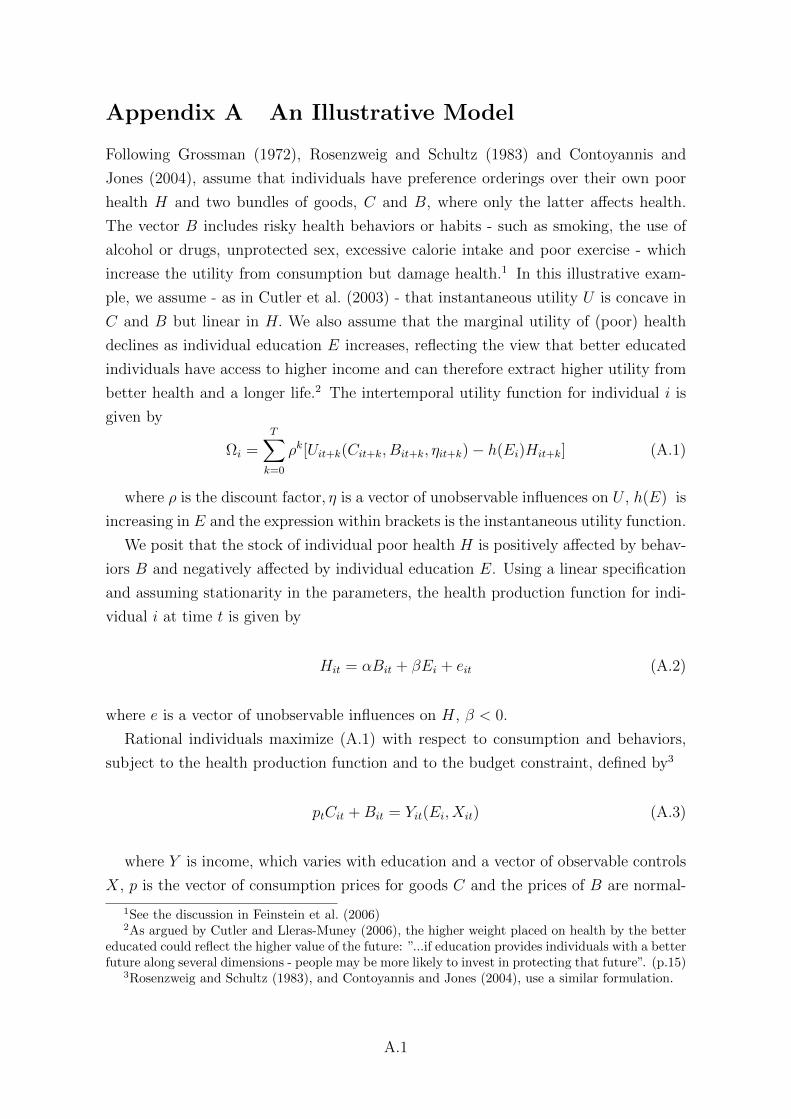
Appendix A An Illustrative Model

Following Grossman (1972), Rosenzweig and Schultz (1983) and Contoyannis and

Jones (2004), assume that individuals have preference orderings over their own poor

health H and two bundles of goods, C and B, where only the latter affects health.

The vector B includes risky health behaviors or habits - such as smoking, the use of

alcohol or drugs, unprotected sex, excessive calorie intake and poor exercise - which

increase the utility from consumption but damage health.1 In this illustrative exam-

ple, we assume - as in Cutler et al. (2003) - that instantaneous utility U is concave in

C and B but linear in H. We also assume that the marginal utility of (poor) health

declines as individual education E increases, reflecting the view that better educated

individuals have access to higher income and can therefore extract higher utility from

better health and a longer life.2 The intertemporal utility function for individual i is

given by

Ωi =T∑k=0

ρk[Uit+k(Cit+k, Bit+k, ηit+k)− h(Ei)Hit+k] (A.1)

where ρ is the discount factor, η is a vector of unobservable influences on U , h(E) is

increasing in E and the expression within brackets is the instantaneous utility function.

We posit that the stock of individual poor health H is positively affected by behav-

iors B and negatively affected by individual education E. Using a linear specification

and assuming stationarity in the parameters, the health production function for indi-

vidual i at time t is given by

Hit = αBit + βEi + eit (A.2)

where e is a vector of unobservable influences on H, β < 0.

Rational individuals maximize (A.1) with respect to consumption and behaviors,

subject to the health production function and to the budget constraint, defined by3

ptCit +Bit = Yit(Ei, Xit) (A.3)

where Y is income, which varies with education and a vector of observable controls

X, p is the vector of consumption prices for goods C and the prices of B are normal-

1See the discussion in Feinstein et al. (2006)2As argued by Cutler and Lleras-Muney (2006), the higher weight placed on health by the better

educated could reflect the higher value of the future: ”...if education provides individuals with a betterfuture along several dimensions - people may be more likely to invest in protecting that future”. (p.15)

3Rosenzweig and Schultz (1983), and Contoyannis and Jones (2004), use a similar formulation.

A.1

ized to 1. Assuming that an internal solution exists, the necessary conditions for a

maximum are

UCit − λpt = 0 (A.4)

UBit + ραh(Ei)− λ = 0 (A.5)

where λ is the Lagrange multiplier and the superscripts are for partial derivatives. By

totally differentiating (A.4) and (A.5) and using (A.2) we obtain that

∂Bit

∂Ei=−ραpt ∂h(Ei)

∂Ei

∆(A.6)

where ∆ is the determinant of the bordered Hessian, which is positive if the second

order conditions for a maximum hold. It follows that higher education reduces optimal

risky behaviors if ∂h(Ei)∂Ei

> 0.

Equations (A.3), (A.4) and (A.5) yield optimal health behaviors

Bit = B(Ei, pt, ρ,Xit, ηit) (A.7)

Using (A.2), (A.7) and a similar expression for consumption C in (A.1) yields the

indirect utility function

Γit = Γ(Ei, pt, ρ,Xit, ηit, eit) (A.8)

Letting Υ(Ei, Qit) be the cost of investing in education, where Q are cost shifters,

the condition

ΓEit = ΥEit (A.9)

defines optimal education, which depends both on health production shocks e and

on preference shocks η.

A.2

Appendix B Synthetic Indicators for Parental Back-

ground

We have built synthetic indicators of parental background by extracting the first prin-

cipal component from several groups of variables, in order to reduce the dimensionality

of the vector of controls. Since most indicators are discrete we use the polychoric or

polyserial correlation matrix instead of the usual correlation matrix as the starting

point of the principal component analysis. The polychoric correlation matrix is a

maximum likelihood estimate of the correlation between ordinal variables which uses

the assumption that ordinal variables are observed indicators of latent and normally

distributed variables. The polyserial correlation matrix is defined in a similar manner

when one of the indicators is ordinal and the others are continuous. We list below the

synthetic indicators, the observed variables used for each indicator and the interpreta-

tion we propose, based on the sign of the scoring coefficients. The scoring coefficients

are the same across males and females (otherwise, we argue, results would not be

comparable and we could not proceed with the aggregation-differentiation strategy).

Poor Housing at 10 based on the number of rooms in the house at age 10 and facil-

ities in the house (hot water) at age 10. The extracted first principal component

decreases as the number of rooms in the house (where the individual lived at age

10) increases and if there was no hot water: we interpret this indicator as poor

housing conditions at age 10 ;

Parents drunk or had mental problems at 10 based on binary indicators of whether

parents drunk or had mental problems when the individual was aged 10. Since

the extracted principal component increases if parents drunk or had mental prob-

lems, we interpret it as poor parental background at age 10 ;

Parental absence at 10 based on three binary indicators: whether the mother died

early, whether the father died early and whether the mother and the father where

present when the individual was aged 10. The extracted principal component

increases if any parent died early and decreases when parents were present at

age 10. We interpret this indicator as poor care at young age.

Descriptive statistics on the background variables used to build the synthetic indi-

cators and the additional background variables used in the baseline specification are

reported in Table B.1.

B.1

Table B.1: Descriptive statistics, baseline estimation sample (micro data), males (M)and females (F).

Country Few books Serious Poor Health Hospital No hot water Roomsat 10 dis. at 15 at 10 at 10 at 10 at 10

M F M F M F M F M F M FAustria 0.42 0.48 0.33 0.32 0.13 0.13 0.11 0.10 0.37 0.37 3.3 3.1Belgium 0.49 0.46 0.27 0.28 0.06 0.09 0.04 0.05 0.30 0.33 5.1 5.2Denmark 0.23 0.24 0.25 0.25 0.08 0.08 0.09 0.09 0.13 0.14 4.4 4.3England 0.30 0.24 0.36 0.31 0.10 0.13 0.11 0.11 0.04 0.21 2.9 3.0France 0.47 0.48 0.29 0.28 0.10 0.13 0.04 0.04 0.24 0.26 4.3 4.0Germany 0.32 0.31 0.30 0.33 0.13 0.12 0.09 0.08 0.10 0.10 3.9 4.0Greece 0.64 0.64 0.21 0.17 0.00 0.00 0.00 0.01 0.38 0.33 2.7 2.8Italy 0.79 0.75 0.16 0.21 0.05 0.08 0.02 0.03 0.47 0.45 3.1 2.9Netherlands 0.35 0.30 0.23 0.22 0.11 0.11 0.08 0.08 0.05 0.04 4.7 4.6Spain 0.66 0.65 0.14 0.17 0.09 0.11 0.02 0.02 0.46 0.44 3.6 3.5Sweden 0.20 0.18 0.24 0.24 0.06 0.08 0.09 0.08 0.14 0.13 3.7 3.6Switzerland 0.28 0.31 0.30 0.32 0.06 0.14 0.07 0.07 0.03 0.05 4.8 4.9All 0.43 0.41 0.27 F 0.08 F 0.07 0.07 0.21 0.21 3.7 3.7

Country Parents Parents Moth/Fath Mother Fatherdrunk at 10 ment. prob. at 10 present at 10 died early died earlyM F M F M F M F M F

Austria 0.09 0.09 0.02 0.02 0.80 0.71 0.0 0.0 0.0 0.0Belgium 0.09 0.09 0.01 0.03 0.92 0.92 0.0 0.0 0.0 0.0Denmark 0.07 0.09 0.08 0.09 0.89 0.90 0.0 0.0 0.0 0.0England 0.05 0.06 0.05 0.06 0.89 0.89 0.01 0.0 0.01 0.01France 0.10 0.10 0.01 0.01 0.90 0.86 0.01 0.01 0.01 0.01Germany 0.07 0.08 0.04 0.05 0.79 0.84 0.0 0.0 0.0 0.0Greece 0.05 0.05 0.00 0.00 0.97 0.97 0.0 0.0 0.0 0.0Italy 0.10 0.11 0.01 0.00 0.92 0.93 0.0 0.0 0.0 0.0Netherlands 0.02 0.05 0.02 0.03 0.92 0.92 0.0 0.0 0.0 0.0Spain 0.08 0.07 0.01 0.01 0.87 0.88 0.0 0.0 0.0 0.0Sweden 0.07 0.08 0.02 0.02 0.87 0.88 0.0 0.0 0.0 0.0Switzerland 0.09 0.09 0.03 0.03 0.91 0.94 0.0 0.0 0.0 0.0All 0.07 0.08 0.03 0.03 0.90 0.90 0.0 0.0 0.01 0.0

B.2

Appendix C Educational Reforms in Europe

In this section, we briefly describe the compulsory schooling reforms we are using in

this study. Our choice of reforms differs somewhat from Brunello, Fabbri and Fort

(2009) and Brunello, Fort and Weber (2009) because the individuals in our data are

aged 50 or older at the time of the interviews in 2004/2006. Therefore, we need to

focus only on relatively early reforms. For further details on educational reforms in

Europe see Fort (2006).

Austria A federal act was passed in 1962 that increased compulsory schooling from

8 to 9 years. The law came into effect on September 1, 1966. Pupils who were 14

years old (or younger) at that time had to attend school for an additional year. Since

compulsory education starts at the age of 6 and the cut-off date for school-entry is

September 1, (mostly) individuals born between September and December 1951 were

the first ones affected by the reform. Thus, the pivotal cohort is 1951.

Czech Republic In the 20th century, compulsory education was reformed several

times. In 1948, compulsory schooling was increased from 8 to 9 years (age 6 to 15).

It was reduced to 8 in 1953 and increased to 9 again in 1960. Two further changes

took place in 1979 and 1990. We consider the first three reforms for our analysis. The

pivotal cohorts are 1934 (for the first reform), 1939 (for the second) and 1947 for the

reform in 1960. See Garrouste (2010) for more information on compulsory schooling

reforms in the Czech Republic.

Denmark Compulsory education was increased in 1958 by 3 years, from 4 to 7. In

1971, compulsory schooling was further increased by 2 years, from 7 to 9. Education

started at age 7, thus pupils who were 11 years old (or younger) in 1958 were poten-

tially affected by the first reform, i.e. children born in 1947 and after. Since our data

only cover individuals 50+ in 2004/2006, we only consider the first reform for this

study.

England Two major compulsory schooling reforms were implemented in the UK in

1947 and 1973. The first reform increased the minimum school leaving age from 14

to 15, the second reform from 15 to 16. Since the school-entry age is 5 in the UK,

compulsory schooling was increased from 9 to 10 years in 1947 and from 10 to 11

years in 1973. Pupils who were 14 years old (or younger) in 1947 were affected by the

first reform, i.e. cohorts born in 1933 and after. Due to the sampling frame of ELSA

(individuals 50+), we only consider the first reform in this study.

France Two education reforms were implemented in France. Compulsory schooling

was increased from 7 to 8 years (age 13 to 14) in 1936 and from 8 to 10 years (age

C.1

14 to 16) in 1959. After a long transition period, the second reform came into effect

in 1967. The first reform affected pupils born 1923 (and after) and the second reform

pupils born 1953 (and after).

Italy In 1963, junior high school became mandatory in Italy and compulsory years of

schooling increased by 3 years (from 5 to 8 years). The first cohort potentially affected

by this reform is the cohort born in 1949.

Netherlands The Netherlands experienced many changes in compulsory education

in the last century. In this paper, we consider three education reforms: in 1942, in

1947 and in 1950 (Levin and Plug, 1999). With the first reform compulsory schooling

was increased from 7 to 8 years, with the second reform it drop back to 7 years and

with the last reform it increased again by 2 years, from 7 to 9. Accordingly, we choose

the cohorts born in 1929, 1933 and 1936 as pivotal cohorts.

C.2

Authors: Giorgio Brunello, Margherita Fort, Nicole Schneeweis, Rudolf Winter-Ebmer

Title: The Causal Effect of Education on Health: What is the Role of Health Behaviors?

Reihe Ökonomie / Economics Series 280

Editor: Robert M. Kunst (Econometrics)

Associate Editors: Walter Fisher (Macroeconomics), Klaus Ritzberger (Microeconomics)

ISSN: 1605-7996

© 2011 by the Department of Economics and Finance, Institute for Advanced Studies (IHS),

Stumpergasse 56, A-1060 Vienna +43 1 59991-0 Fax +43 1 59991-555 http://www.ihs.ac.at

ISSN: 1605-7996