The Career Cost of Children

Jerome Adda ∗

Christian Dustmann†

Katrien Stevens‡

PRELIMINARY & INCOMPLETE

AbstractThis paper evaluates the life-cycle career costs associated with

childrearing and decomposes its effects between unearned wages aswomen drops out of the labor market, loss of human capital and theselection into more child friendly occupations. We develop a dynamiclife-cycle model of fertility and career choice. The model allows forthe endogenous timing of births and number of children, labor mar-ket participation, hours of work, wages and selection into differentoccupation. We structurally estimate this model combining detailedsurvey and administrative data for Germany. We identify the modelusing differential changes in regional availability of training positionsover time during adolescence, which displace young girls into differentoccupations.

1 Introduction

The past century has seen a significant increase in labor market participation

of women, with participation rates of mothers with young children increas-

ing the most. During the same period, fertility rates have declined in many

∗European University Institute.†University College London.‡University of Sydney. Funding through the ESRC grant RES-000-22-0620 is gratefully

acknowledge. We would like to thank Michael Keane, Costas Meghir, Derek Neal, Jean-Marc Robin and seminar participants at Autonoma- Barcelona, the Chicago Fed, IFS,Mannheim, Northwestern, the NBER Labor Summer Meetings and Sciences Po-Paris forhelpful comments.

1

developed countries and women have delayed the arrival of their first child.

To understand the dependencies between female participation decisions, oc-

cupational choices, wage dynamics and labor supply on the one hand and

the fertility decision and the timing of births on the other, recognizing that

joint nature of career planing and fertility, is difficult, as it involves a number

of identification problems. Nevertheless, it is key to answer many important

public policy questions.

There is a large literature which studies female careers over the life-cycle,

but considering fertility decisions as exogenous. 1 Important examples are

Mincer and Polachek (1974), Heckman and Macurdy (1980), Eckstein and

Wolpin (1989), van der Klaauw (1996), Altug and Miller (1998) and Attana-

sio, Low, and Sanchez-Marcos (2004) 2. These studies emphasize the role of

previous labor market experience on labor market status and wages. They

also emphasize the importance of child care costs as determinants of female

labor supply. Other papers investigate fertility decisions of females, largely

in isolation from their career decisions (Newman and McCulloch (1984)).

Few papers have modeled jointly fertility decisions and labor market

choices. Hotz and Miller (1988) develop a life cycle model of fertility and

female labor supply. However their model makes no connection between

wages and fertility apart from the extensive margin in labor supply deci-

sions. Francesconi (2002) also derives a joint model of fertility and career

choices, emphasizing the choice of part-time work. 3

In the seminal contributions of Becker (1960) and Becker and Lewis

(1973), a mother derives utility from consumption, the number of her chil-

1A number of papers study the career of men such as Keane and Wolpin (1997).2However, their model incorporate savings decisions3Reduced-form studies investigating wages and fertility include Moffitt (1984) and

Heckman and Walker (1990).

2

dren and their quality. Fertility is the result of the optimization of the utility,

subject to a standard budget constraint. We build on this literature by ex-

tending this model in several important directions. We place this choice in

a dynamic and life-cycle perspective, where women chose also their labor

supply and acquire (and lose) human capital. In addition, we also allow for

heterogeneity in occupations, where women face a trade-off between higher

wages or wage growth against more child-friendly occupations.

This paper draws on this previous literature to combine a model of career

and fertility choices. Due to the dynamic nature of the decisions concerning

these outcomes, we cannot rely on reduced form models. Our model allows

for the endogenous timing of births and the number of children, as well as

labor market participation, number of hours worked and wage progression.

We model in addition occupational choice and how it interferes with fertility

and wages. 4 In particular, following Mincer and Polachek (1974) and Mincer

and Olfek (1982) we investigate how the loss of human capital following inter-

ruptions due to maternity leave shape fertility decisions across occupational

groups. Rosenzweig and Schultz (1985) show that unexpected births, seen as

exogenous shocks to fertility, have an impact on labor market participation

and wages. Goldin and Katz (2002) have shown how (exogenous) changes

in fertility, the diffusion of oral birth control pills, have changed education

and career choices. We investigate the opposite relationship, considering how

shocks to occupational choices affect subsequent fertility and career decisions.

Our analysis is for Germany. We consider career choices of young women

aged 15 or 16, and who choose apprenticeship education. This is about 60

percent of each cohort. The remaining 40 percent either join the labour

market directly, or continue with high school education. Important is that

4The occupational segregation by sex has been emphasized by Polachek (1981).

3

the choice of school track in Germany is made earlier (at the age of 10).

When enrolling in apprenticeship training (which usually lasts for about 3

years), women have to choose a particular apprenticeship occupation. There

are about 360 registered apprenticeship occupations to chose from. Occupa-

tions range from craft (like carpenter) over services (like shop assistant or

hairdresser) to medical (like medical assistant) to white collar occupations

(like bank clerk). Occupations differ in their wage paths, as well as in the

loss of human capital they imply when leaving the work force for a period.

Although occupational changes are possible, and do occur, they are costly.

Thus, this setting allows us to observe occupational choices of a large fraction

of the female labour force at the earliest possible stage.

Another distinctive feature of our approach is that we combine data from

a large number of cohorts who enter the labor market at different points

in the business cycle and in different local labor markets, as in Adda, Dust-

mann, Meghir, and Robin (2006). This is an important advantage of our data

over other sources such as the NLSY, which in essence follows one cohort of

individuals. Thus controlling for time trends and for permanent regional

effects, we use the differential changes in the availability of apprenticeship

occupations as a source of identification within our structural model: Dif-

ferent regions include different concentrations of industry. As product prices

fluctuate so does the local demand for labor and for apprenticeships, depend-

ing how the local industry is affected. While trade ensures local wages do not

react to such shocks the number of apprenticeship positions will adjust. This

argument provides us both with the required exogenous variation and with

exclusion restrictions required to identify the effect of occupational choices

on fertility. Using a difference in differences approach, we demonstrate in the

descriptive part of the paper that the variation we use is indeed informative

4

as far as occupational choices are concerned.

The paper proceeds as follows. Section 2 presents the data set. Section 3

presents the model. Section 4 presents the estimation methods and parameter

estimates. Section 5 evaluates the effect of fertility on careers. Finally,

Section 6 concludes.

2 The Data

The description of individual behaviour of females in terms of career and

fertility relies on 2 different datasets: (1) the IAB Employment subsample:

employment register data, for the period 1975-2001 and (2) the German

Socio-Economic Panel (GSOEP): a German household panel survey, cover-

ing the period 1984-2003. Each dataset provides information about specific

aspects of the career-fertility process. The IAB data provide information on

the wage profile and transitions in and out of work, while the GSOEP data

mainly supply information about the fertility process and the (yearly) work

behaviour of females after birth.

2.1 IAB Employment Sample

The first dataset is provided by the German Institute for Employment Re-

search (IAB5). It is a 1% random sample drawn from German social security

records, to which all employers have to report about any employees covered

by the social security system. These notifications are required at the end of

each year and whenever an employment relationship is started or completed.

The reports include information on aspects as exact start and end date of

5Institut fuer Arbeitsmarkt- und Berufsforschung, Nuremberg (Institute for Employ-

ment Research).

5

a work contract, year of birth, gender, nationality, occupation, qualification

and gross daily earnings of the employee6. Furthermore, each spell includes

some information on the industry and the firm in which an individual is em-

ployed. The data provides a continuous employment history for each of the

included employees over the period 1975-2001. The definition of the regis-

ter database implies that civil servants and self-employed persons are not

observed in the data. Note also that work spells with earnings below the

earnings threshold do not require payment of social security contributions

and are therefore also not present in the data. Finally, individuals working

in East-Germany (before 1992) or abroad are not included. This 1% sample

contains around 20 million observed spells, for +/- 2.5 million individuals.7

The sample drawn from this dataset includes females in West-Germany

who have undertaken vocational training within the dual apprenticeship pro-

gramme in the period 1976-2001, but did not continue into higher educa-

tion8,9. Typically, they have completed 9-10 years of schooling and 2-3 years

of apprenticeship. The detailed information by spell (with variable duration)

is transformed into observations per quarter. The sample contains 72430

women, born between 1955-1975, observed from entry into the labour mar-

ket (LM) onwards to 2001, i.e. for some time between age 15 and Descriptive

information is shown in the top panel of table 18. This sample is mainly used

for information about the wage profile and transitions between the work/not

work states. A unique aspect of the IAB data is that work histories can be

observed from the start and that there is very detailed information about

6Gross daily earnings reflect an average daily wage for the period worked in a firm (up

to one year).7For more info on the dataset, see Bender et al.(2000).8Apprenticeship training is observed in the data.9In addition, our sample requires engaging in apprenticeship training before age 22.

6

labour market experiences. Remark, however, that this type of data does

not provide information on household characteristics such as income and

employment of the partner.

2.2 GSOEP data

The GSOEP is a longitudinal survey of private households and persons in

Germany, which started in 1984. It is a representative sample of households

living in Germany with detailed information about socio-economic variables

on a yearly basis. The dataset provides information on population, demog-

raphy, education, training, qualification, labour market and occupational

dynamics, earnings, income, social security, housing, health and household

production. The first wave (1984) included almost 6000 households and more

than 12000 respondents.10

A sample is chosen to obtain information on total fertility and labour

market behaviour of women. As in the IAB sample, we focus our attention

on women who obtain an apprenticeship degree, but do not take higher edu-

cation; individuals who work as civil servants or self-employed individuals are

dropped. Parallel to the sample from the IAB data, only women of the birth

cohorts 1955-1975 are included. We retain information about year of birth,

employment status, part time or full time work, actual and agreed hours of

work (per week), occupation, gross and net individual earnings, education

level, number of children and year of birth of children. Based on 23 waves

of GSOEP data (1984-2006), our sample contains a total of 16144 successful

interviews, from 1432 women. The youngest women in our sample are ob-

served at age 17, while the oldest women are aged 51. We observe at least

10A detailed description of the data set can be found in Haisken-DeNew and Frick (2003)

7

500 women at each age between 21-38. For 50% of the women we have data

from 10 or more successful interviews. There are more than 1000 births in

the sample and about 9700 work spells (after apprenticeship)11. Most of the

latter have net and gross individual earnings reported. Further descriptive

information is provided in panel B of table 18.12

2.3 Construction of task-based occupations

The analysis relies on an occupational classification which reflects the task-

content of jobs: routine, abstract and manual occupations. This classification

relies on the task-based framework introduced by Autor, Levy, and Murnane

(2003). The advantage is that it allows us to classify jobs according to a cru-

cial element in our model: occupational skill requirements. Note also that

the task-based approach is growing in importance in labor market research.

The occupational grouping is constructed using survey data provided by the

Federal Institute for Vocational Education and Training Germany (Bundesin-

stitut fur Berufsbildung - BIBB). The German Qualification and Career Sur-

vey (Qualifikation und Berufsverlauf 1985/86) includes information on tasks

reported on the job, and is representative for the West-German active labor

force aged 15-65. This data has also been used by Gathmann and Schonberg

(2010) and Black and Spitz-Oener (2010) to develop task-based indicators of

occupations in their analysis of the German labor market. The reported tasks

11Note that some women report doing ’irregular PT work’ in the GSOEP data. Given

the rather low frequency of this status and given that we do not observe this status in the

IAB data, we choose to classify this type of work as not working.12Earnings in both the IAB and GSOEP samples have been (1) deflated using the

Consumer Price Index for private households, obtained from the German Statistical Office,

and (2) have been converted into Euros.

8

are assigned to a particular type: routine, abstract or manual.13 Task inten-

sity indicators are then constructed at 2-digit level jobs and each of these jobs

is categorized as involving mainly routine, abstract or manual tasks. This

classification is applied to our data samples from GSOEP and IABS data.

Shop assistants, sewers, cooks, assemblers and cleaners are classified as rou-

tine occupations. Abstract occupations contain positions such as secretaries,

office clerks, bank professionals, stenographers, accountants and social work-

ers. Finally, manual occupations include jobs in nursing, hairdressing, but

also consultation hour assistants, waiters and stewards. For more details, see

appendix C.

2.4 Wages, hours of work and fertility in the data

This section presents descriptive evidence on occupations, work behaviour

and fertility from both datasets. We distinguish between 3 occupations as

detailed above, which are predominantly routine, abstract or manual.

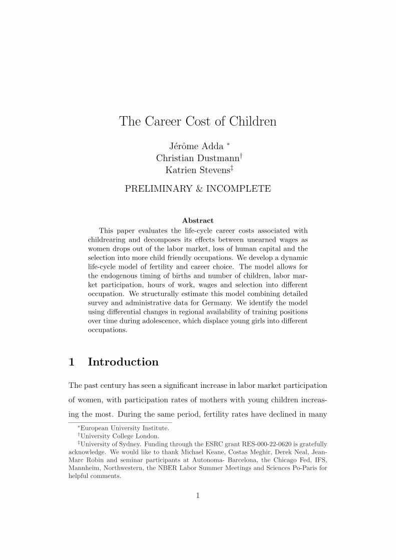
Figure 1 shows the wage-experience profile for each of the occupations14.

Daily earnings in abstract jobs are the highest for any level of experience,

followed by manual and routine ones.

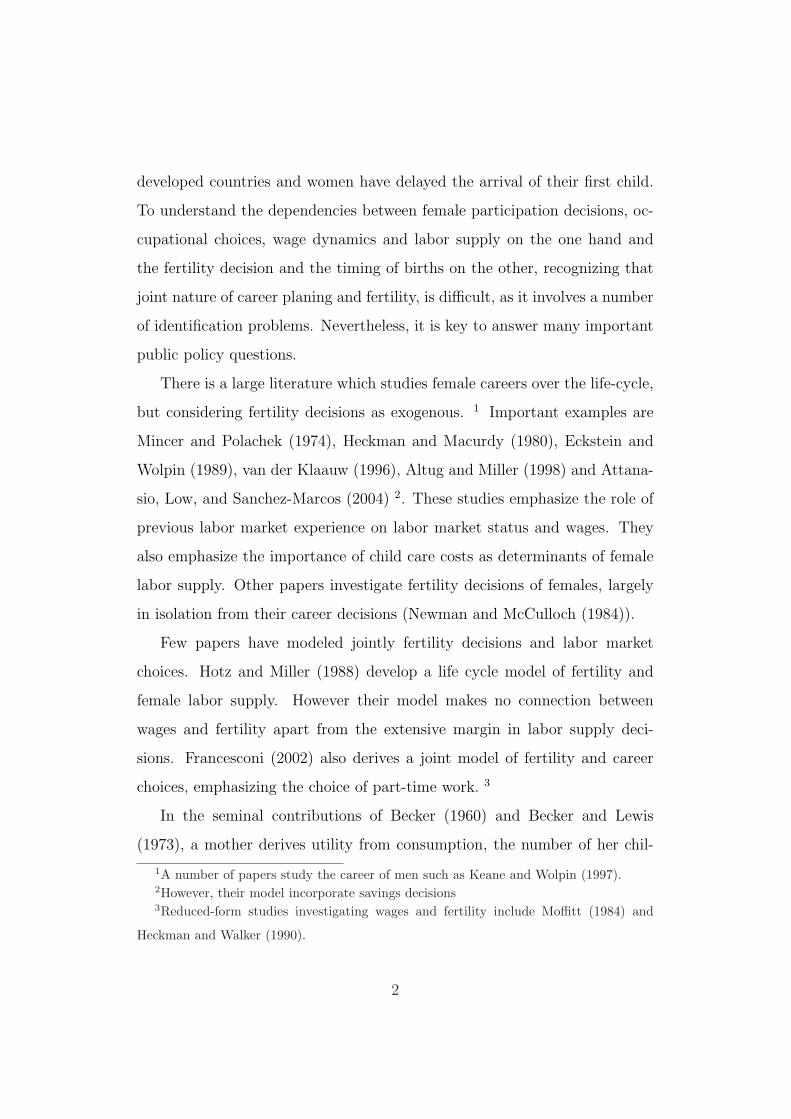
Figure 2 displays the labor market status by occupation and at three

different ages, 30, 35 and 40. The proportion of women in full time work

ranges between 20% and 45%. Women spend also a considerable amount of

time out of the labor force, ranging from 40 to 60%. Part time work increases

with age in all occupations. Women in abstract jobs spend more time working

at all ages. Experience accumulation by occupation is illustrated in figure

13We are grateful to Marco Hafner at the Institute for Employment Research (IAB) for

help with constructing the task-content of jobs.14Average daily wages are shown from 2 years of experience onwards, as the first 2-3

years are spent in apprenticeship - with very low wages

9

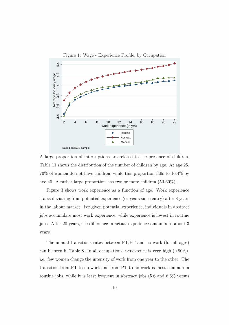
Figure 1: Wage - Experience Profile, by Occupation3.

43.

63.

84

4.2

4.4

Ave

rage

log

daily

wag

e

2 4 6 8 10 12 14 16 18 20 22work experience (in yrs)

Routine

Abstract

Manual

Based on IABS sample

A large proportion of interruptions are related to the presence of children.

Table 11 shows the distribution of the number of children by age. At age 25,

70% of women do not have children, while this proportion falls to 16.4% by

age 40. A rather large proportion has two or more children (50-60%).

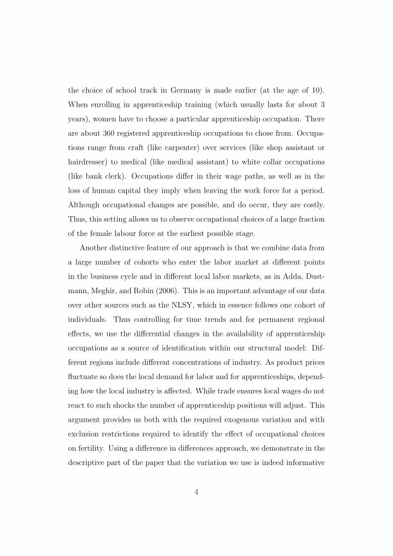
Figure 3 shows work experience as a function of age. Work experience

starts deviating from potential experience (or years since entry) after 8 years

in the labour market. For given potential experience, individuals in abstract

jobs accumulate most work experience, while experience is lowest in routine

jobs. After 20 years, the difference in actual experience amounts to about 3

years.

The annual transitions rates between FT,PT and no work (for all ages)

can be seen in Table 8. In all occupations, persistence is very high (>90%),

i.e. few women change the intensity of work from one year to the other. The

transition from FT to no work and from PT to no work is most common in

routine jobs, while it is least frequent in abstract jobs (5.6 and 6.6% versus

10

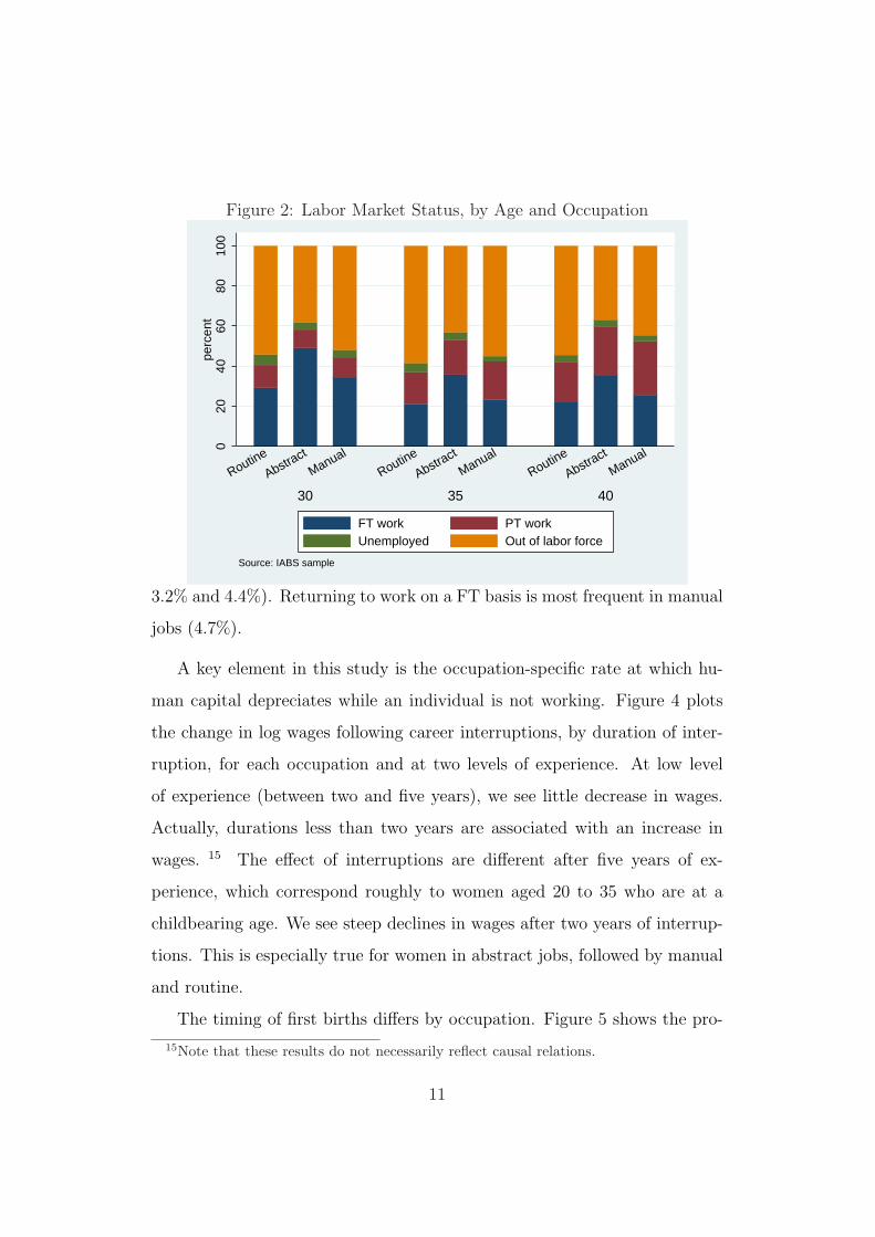
Figure 2: Labor Market Status, by Age and Occupation0

2040

6080

100

perc

ent

30 35 40

Routine

Abstract

Manual

Routine

Abstract

Manual

Routine

Abstract

Manual

Source: IABS sample

FT work PT workUnemployed Out of labor force

3.2% and 4.4%). Returning to work on a FT basis is most frequent in manual

jobs (4.7%).

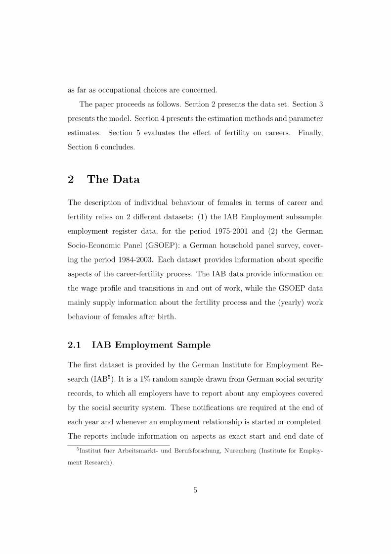
A key element in this study is the occupation-specific rate at which hu-

man capital depreciates while an individual is not working. Figure 4 plots

the change in log wages following career interruptions, by duration of inter-

ruption, for each occupation and at two levels of experience. At low level

of experience (between two and five years), we see little decrease in wages.

Actually, durations less than two years are associated with an increase in

wages. 15 The effect of interruptions are different after five years of ex-

perience, which correspond roughly to women aged 20 to 35 who are at a

childbearing age. We see steep declines in wages after two years of interrup-

tions. This is especially true for women in abstract jobs, followed by manual

and routine.

The timing of first births differs by occupation. Figure 5 shows the pro-

15Note that these results do not necessarily reflect causal relations.

11

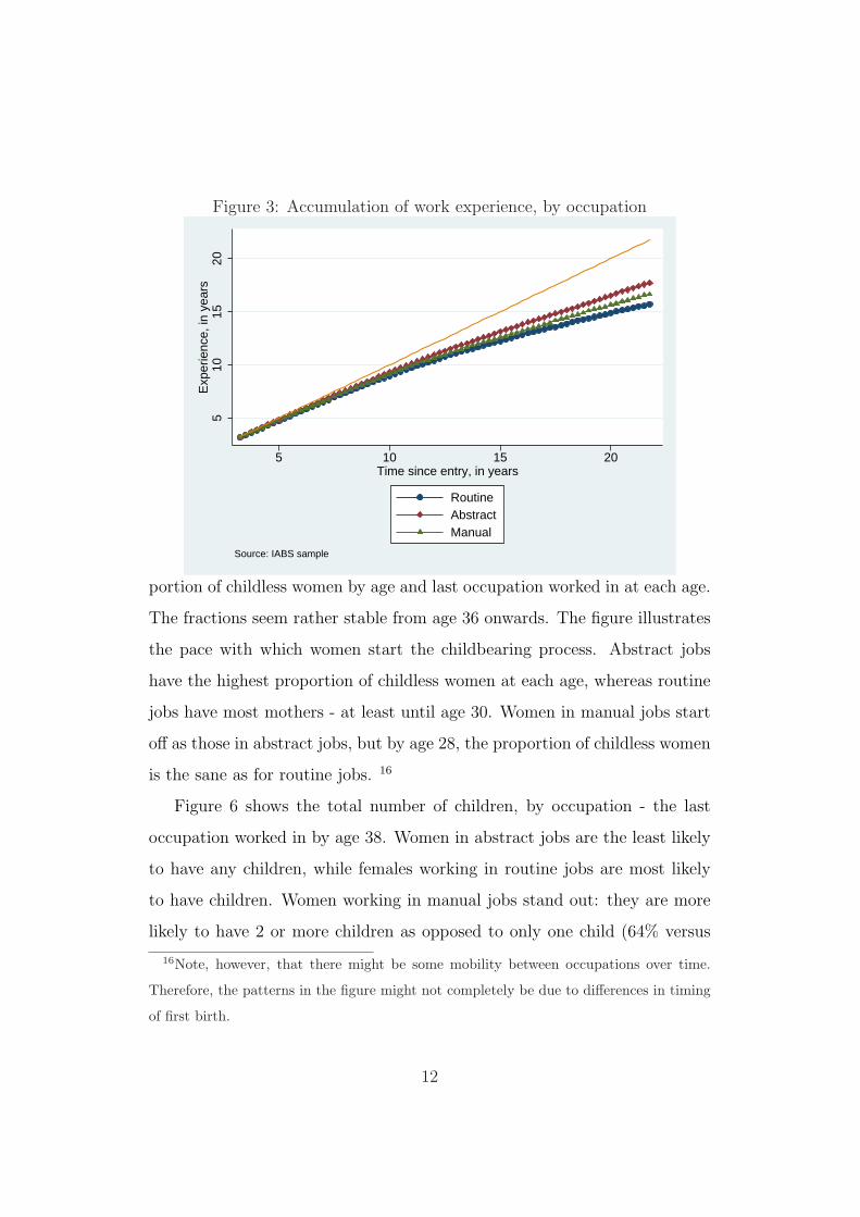
Figure 3: Accumulation of work experience, by occupation5

1015

20E

xper

ienc

e, in

yea

rs

5 10 15 20Time since entry, in years

RoutineAbstractManual

Source: IABS sample

portion of childless women by age and last occupation worked in at each age.

The fractions seem rather stable from age 36 onwards. The figure illustrates

the pace with which women start the childbearing process. Abstract jobs

have the highest proportion of childless women at each age, whereas routine

jobs have most mothers - at least until age 30. Women in manual jobs start

off as those in abstract jobs, but by age 28, the proportion of childless women

is the sane as for routine jobs. 16

Figure 6 shows the total number of children, by occupation - the last

occupation worked in by age 38. Women in abstract jobs are the least likely

to have any children, while females working in routine jobs are most likely

to have children. Women working in manual jobs stand out: they are more

likely to have 2 or more children as opposed to only one child (64% versus

16Note, however, that there might be some mobility between occupations over time.

Therefore, the patterns in the figure might not completely be due to differences in timing

of first birth.

12

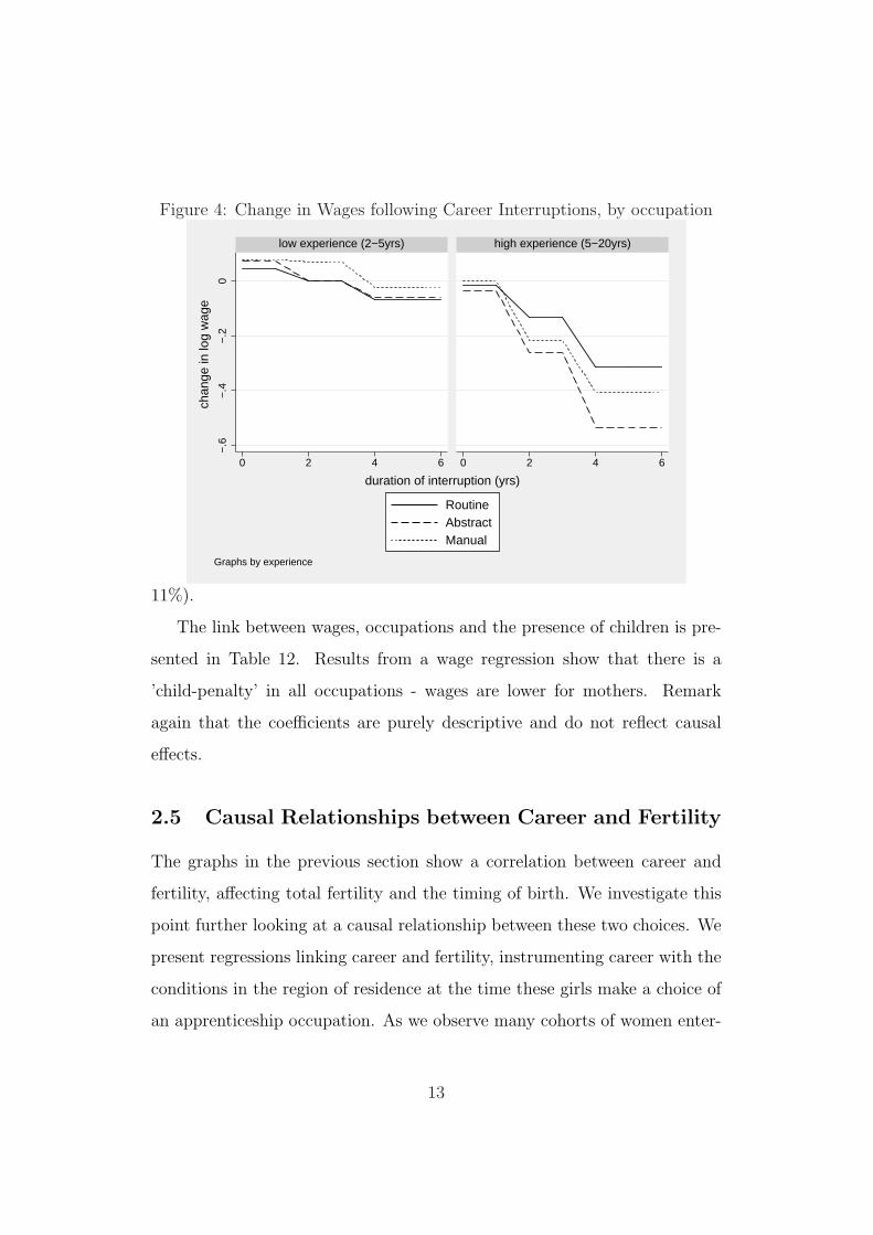
Figure 4: Change in Wages following Career Interruptions, by occupation−

.6−

.4−

.20

0 2 4 6 0 2 4 6

low experience (2−5yrs) high experience (5−20yrs)

RoutineAbstractManual

chan

ge in

log

wag

e

duration of interruption (yrs)

Graphs by experience

11%).

The link between wages, occupations and the presence of children is pre-

sented in Table 12. Results from a wage regression show that there is a

’child-penalty’ in all occupations - wages are lower for mothers. Remark

again that the coefficients are purely descriptive and do not reflect causal

effects.

2.5 Causal Relationships between Career and Fertility

The graphs in the previous section show a correlation between career and

fertility, affecting total fertility and the timing of birth. We investigate this

point further looking at a causal relationship between these two choices. We

present regressions linking career and fertility, instrumenting career with the

conditions in the region of residence at the time these girls make a choice of

an apprenticeship occupation. As we observe many cohorts of women enter-

13

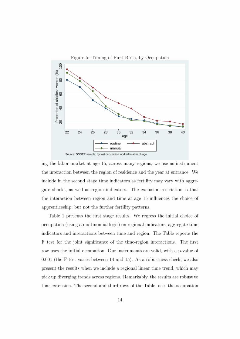
Figure 5: Timing of First Birth, by Occupation20

4060

8010

0P

ropo

rtio

n of

chi

ldle

ss w

omen

(%

)

22 24 26 28 30 32 34 36 38 40age

routine abstractmanual

Source: GSOEP sample, by last occupation worked in at each age

ing the labor market at age 15, across many regions, we use as instrument

the interaction between the region of residence and the year at entrance. We

include in the second stage time indicators as fertility may vary with aggre-

gate shocks, as well as region indicators. The exclusion restriction is that

the interaction between region and time at age 15 influences the choice of

apprenticeship, but not the further fertility patterns.

Table 1 presents the first stage results. We regress the initial choice of

occupation (using a multinomial logit) on regional indicators, aggregate time

indicators and interactions between time and region. The Table reports the

F test for the joint significance of the time-region interactions. The first

row uses the initial occupation. Our instruments are valid, with a p-value of

0.001 (the F-test varies between 14 and 15). As a robustness check, we also

present the results when we include a regional linear time trend, which may

pick up diverging trends across regions. Remarkably, the results are robust to

that extension. The second and third rows of the Table, uses the occupation

14

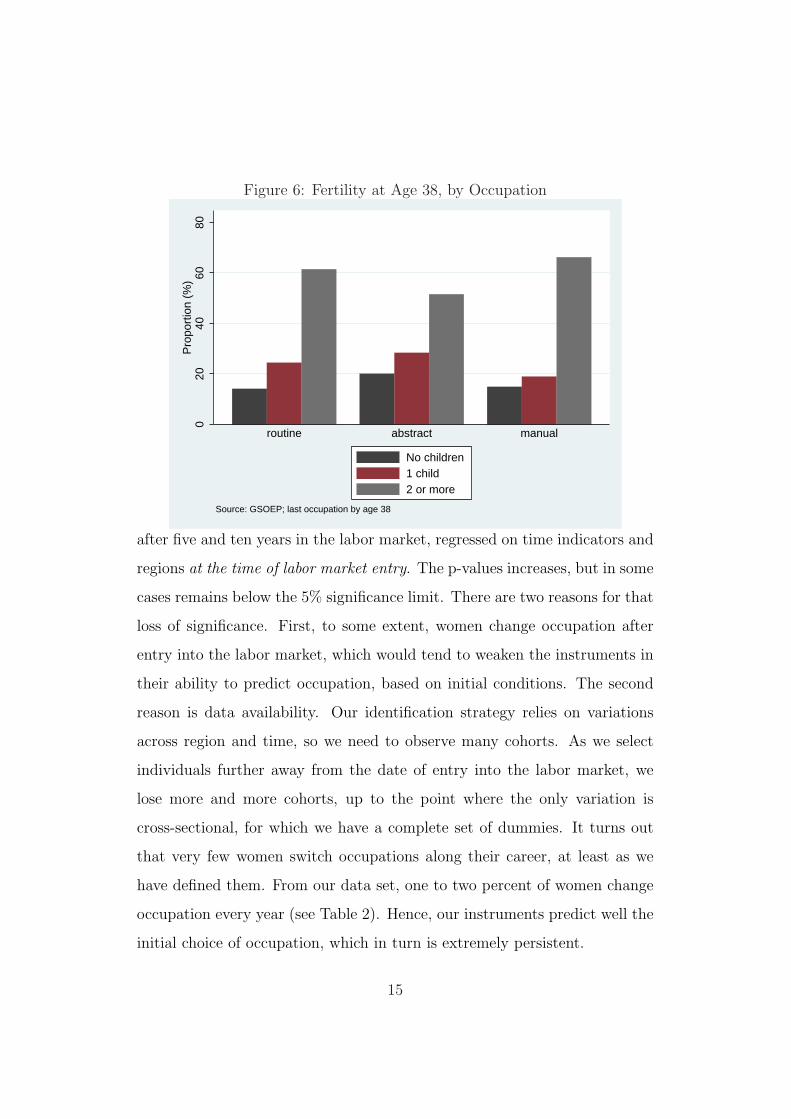
Figure 6: Fertility at Age 38, by Occupation0

2040

6080

Pro

port

ion

(%)

routine abstract manual

Source: GSOEP; last occupation by age 38

No children1 child2 or more

after five and ten years in the labor market, regressed on time indicators and

regions at the time of labor market entry. The p-values increases, but in some

cases remains below the 5% significance limit. There are two reasons for that

loss of significance. First, to some extent, women change occupation after

entry into the labor market, which would tend to weaken the instruments in

their ability to predict occupation, based on initial conditions. The second

reason is data availability. Our identification strategy relies on variations

across region and time, so we need to observe many cohorts. As we select

individuals further away from the date of entry into the labor market, we

lose more and more cohorts, up to the point where the only variation is

cross-sectional, for which we have a complete set of dummies. It turns out

that very few women switch occupations along their career, at least as we

have defined them. From our data set, one to two percent of women change

occupation every year (see Table 2). Hence, our instruments predict well the

initial choice of occupation, which in turn is extremely persistent.

15

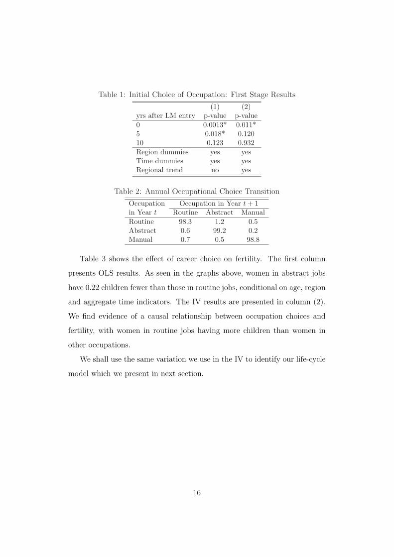
Table 1: Initial Choice of Occupation: First Stage Results

(1) (2)yrs after LM entry p-value p-value0 0.0013* 0.011*5 0.018* 0.12010 0.123 0.932Region dummies yes yesTime dummies yes yesRegional trend no yes

Table 2: Annual Occupational Choice Transition

Occupation Occupation in Year t + 1in Year t Routine Abstract ManualRoutine 98.3 1.2 0.5Abstract 0.6 99.2 0.2Manual 0.7 0.5 98.8

Table 3 shows the effect of career choice on fertility. The first column

presents OLS results. As seen in the graphs above, women in abstract jobs

have 0.22 children fewer than those in routine jobs, conditional on age, region

and aggregate time indicators. The IV results are presented in column (2).

We find evidence of a causal relationship between occupation choices and

fertility, with women in routine jobs having more children than women in

other occupations.

We shall use the same variation we use in the IV to identify our life-cycle

model which we present in next section.

16

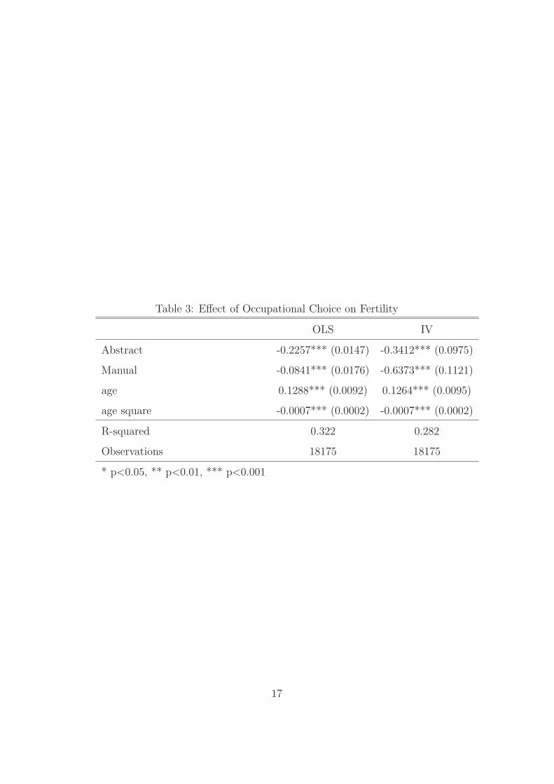
Table 3: Effect of Occupational Choice on Fertility

OLS IV

Abstract -0.2257*** (0.0147) -0.3412*** (0.0975)

Manual -0.0841*** (0.0176) -0.6373*** (0.1121)

age 0.1288*** (0.0092) 0.1264*** (0.0095)

age square -0.0007*** (0.0002) -0.0007*** (0.0002)

R-squared 0.322 0.282

Observations 18175 18175

* p<0.05, ** p<0.01, *** p<0.001

17

3 A Life-Cycle Model of Fertility and Careers

Our model takes individuals from late adolescence into the end of their work-

ing careers and focus on their occupational choices, labor supply decisions as

well as fertility choices (number of children and spacing of births).

A period in the model lasts six months. In each period, a woman has to

decide whether to conceive a child or not. The chance of conception depends

on the age of the mother, declining after age 35 and virtually zero at age 45,

in accordance with medical evidence. The agent also has a choice of labor

supply and occupation.

Women make decisions about labor supply and fertility conditional on a

number of characteristics. These are their age, ageM , the amount of human

capital, X, the previous occupation, O, previous labor supply decision, L, the

number of children at the start of the period, N , the age of the youngest child,

ageK and the presence of a husband within the household, H. Husbands do

not make choices in the model. They provide a source of income in each

period and provide help to raise children.

We collect these variables into a vector, which we denote Ω. The la-

bor supply indicator takes only three modalities, whether the agent is not

working, working part time or full time.

Utility Function The agent derives utility from consumption, the number

of children and leisure. Raising children requires maternal inputs, which

are taken from working time. Hence mothers have a trade-off between the

quantity of children and lower consumption. Husbands provide also help

with the children, which allows the mother to work more.

We impose a linear utility of consumption and abstract from the choice of

savings. Hence, consumption equals household income. Household income is

18

the sum of the income of the mother and the labor earnings of the husband,

if present. The income of the mother is composed either of labor earnings,

unemployment benefits or maternity benefits, depending on her job market

status.

As in Becker and Lewis (1973), the mother derives utility from the num-

ber of children. The utility of children is interacted with the presence of a

husband, to allow for the possibility that children are more desirable when

a father is present. Children also affect the utility of leisure of the mother,

especially when they are young. We also allow for an interaction between

children, leisure and occupation. This allows us to capture i) the fact that

women have to go part time or drop out of the labor market when having

children, as they require maternal time inputs17; ii) the fact that some oc-

cupations are more child-friendly than others, so that women are less prone

to drop out of the labor market when raising children. Finally, we allow for

heterogeneity in the taste for children, which we denote by ε. This taste

shifter is known to the agent, but unobserved by the econometrician. We

denote the utility function:

u(y,N, L, ageK , O, H, ε)

where y is total household income.

Occupation, Hours of Work and Human Capital Accumulation

Employment is characterized by working in one of the three following types

of jobs, ”manual”, ”routine” or ”abstract” 18, and a particular number of

hours (full time or part time). An occupation is characterized by a particu-

17Note that we do not model the quality of children, as we do not have data on that

outcome.18See Section 2 for a more detailed description on occupation classification

19

lar wage path, a specific skill depreciation process when out of work as well as

being more or less child-friendly. As explained above, we capture the latter

through interactions between occupation, leisure and children in the utility

function.

In each period, the agent may choose an occupation and hours of work (no

work, part time or full time). New offers consisting of a specific occupation

and hours of work arrive randomly in each period. Combining occupation

and hours of work gives us three times two (part time or full time) possible

offers. The probability of receiving an offer of occupation-hours of work

j = 1, . . . , 6 while in occupation/hours of work i is noted φij. While working,

the agent accumulates human capital. We normalize this gain to one for a

period of full time work and λ ∈ [0, 1] for part time work. While out of

work, this human capital depreciates. The rate of depreciation or atrophy

rate, depends on the occupation of the agent and the previous level of human

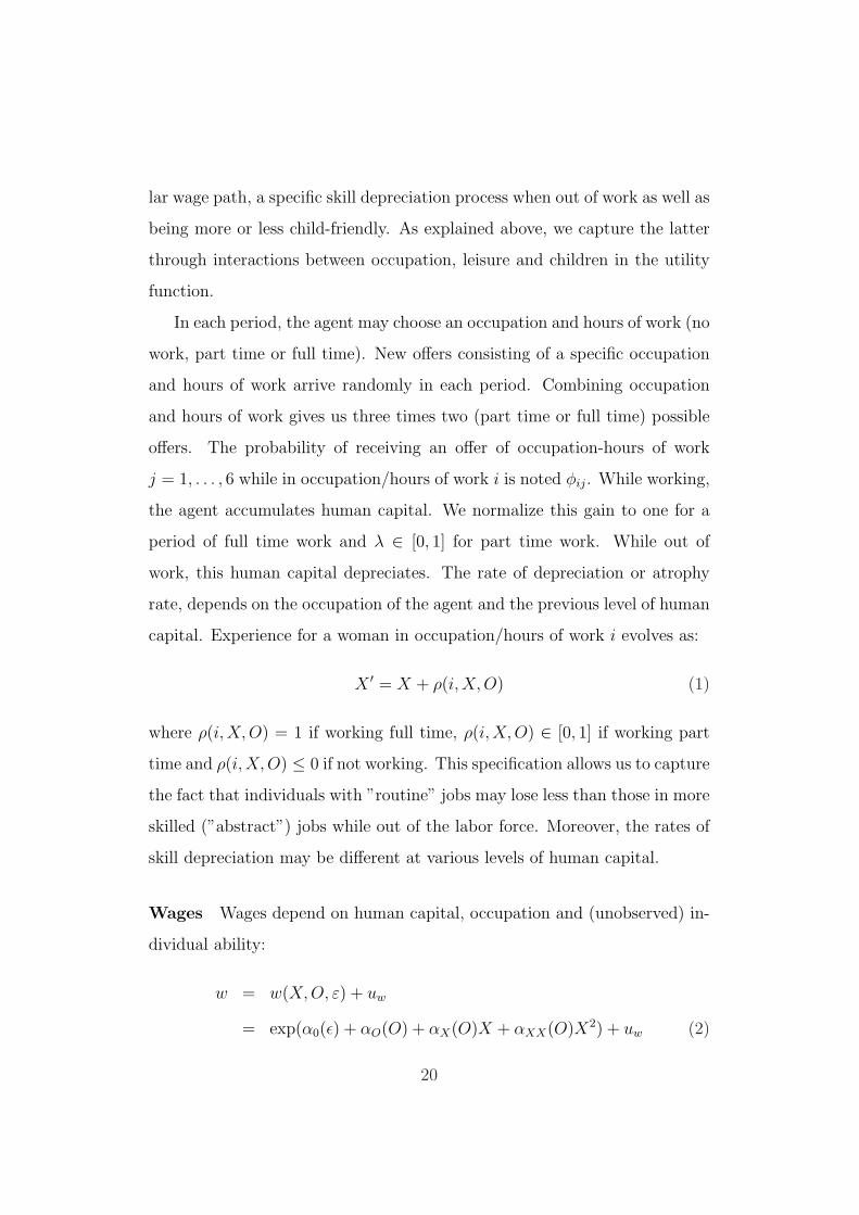
capital. Experience for a woman in occupation/hours of work i evolves as:

X ′ = X + ρ(i, X,O) (1)

where ρ(i,X, O) = 1 if working full time, ρ(i,X, O) ∈ [0, 1] if working part

time and ρ(i,X, O) ≤ 0 if not working. This specification allows us to capture

the fact that individuals with ”routine” jobs may lose less than those in more

skilled (”abstract”) jobs while out of the labor force. Moreover, the rates of

skill depreciation may be different at various levels of human capital.

Wages Wages depend on human capital, occupation and (unobserved) in-

dividual ability:

w = w(X,O, ε) + uw

= exp(α0(ε) + αO(O) + αX(O)X + αXX(O)X2) + uw (2)

20

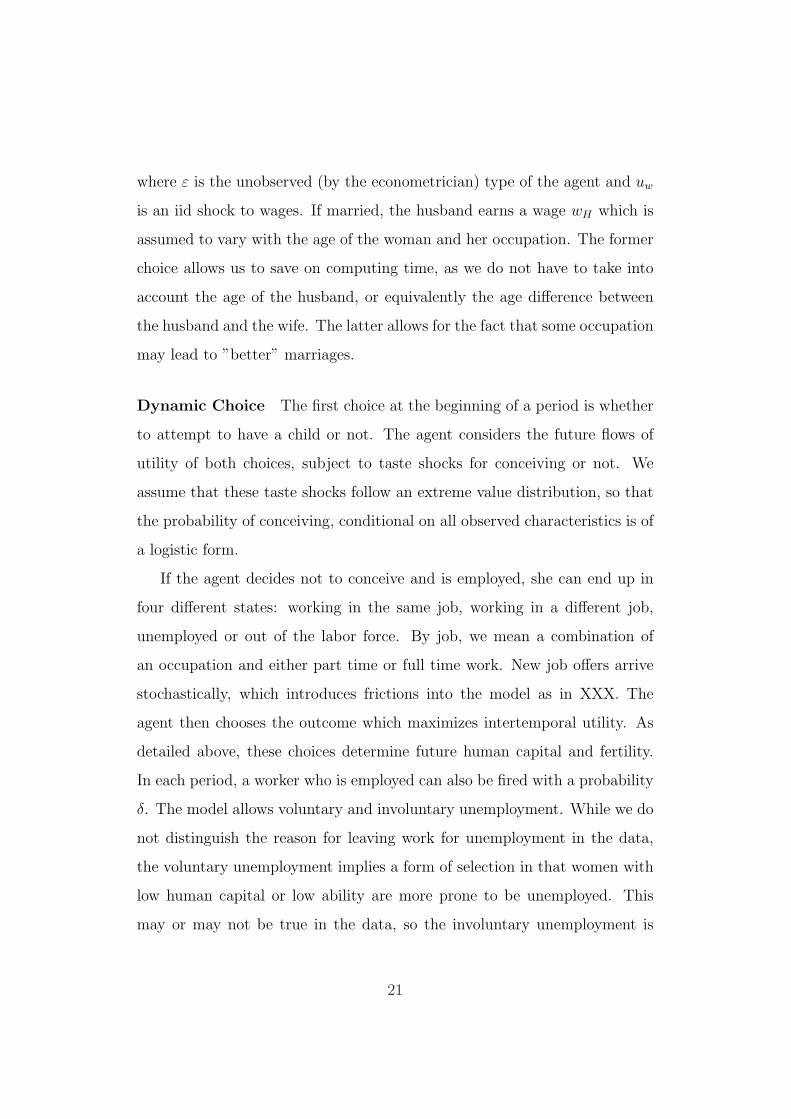
where ε is the unobserved (by the econometrician) type of the agent and uw

is an iid shock to wages. If married, the husband earns a wage wH which is

assumed to vary with the age of the woman and her occupation. The former

choice allows us to save on computing time, as we do not have to take into

account the age of the husband, or equivalently the age difference between

the husband and the wife. The latter allows for the fact that some occupation

may lead to ”better” marriages.

Dynamic Choice The first choice at the beginning of a period is whether

to attempt to have a child or not. The agent considers the future flows of

utility of both choices, subject to taste shocks for conceiving or not. We

assume that these taste shocks follow an extreme value distribution, so that

the probability of conceiving, conditional on all observed characteristics is of

a logistic form.

If the agent decides not to conceive and is employed, she can end up in

four different states: working in the same job, working in a different job,

unemployed or out of the labor force. By job, we mean a combination of

an occupation and either part time or full time work. New job offers arrive

stochastically, which introduces frictions into the model as in XXX. The

agent then chooses the outcome which maximizes intertemporal utility. As

detailed above, these choices determine future human capital and fertility.

In each period, a worker who is employed can also be fired with a probability

δ. The model allows voluntary and involuntary unemployment. While we do

not distinguish the reason for leaving work for unemployment in the data,

the voluntary unemployment implies a form of selection in that women with

low human capital or low ability are more prone to be unemployed. This

may or may not be true in the data, so the involuntary unemployment is

21

identified by the extent of selection into unemployment.

If the agent decides to conceive, a child is born in the next period, with

a probability π(ageM). The mother is then on maternity leave and is then

entitled to maternity benefits. At the end of the maternity leave period, she

has the possibility to get back to the same job as before birth. She may also

receive an alternative job offer, or choose to be unemployed or out of the

labor force.

While unemployed, the agent is entitled to unemployment benefits, and

can either accept a job offer if one arrives, stay unemployed or move out of

the labor force. While out of the labor force, the agent does not receive any

benefits, but enjoys leisure, especially if young children are present.

We refer the reader to a more detailed and formal description in Ap-

pendix A.

Unobserved Heterogeneity As discussed above, the model allows for

fixed unobserved heterogeneity in ability and in desired fertility. This het-

erogeneity is introduced as in Heckman and Singer (1984), using discrete

mass points, which are estimated together with the relative proportion in

the sample. We allow for two ability types, through different intercepts in

the wage equation and two types in desired fertility, through differences in

the utility of the number children. We also allow for a fraction of women to

be unable to conceive (although they do not anticipate that fact).

Initial Choice of Occupation At age 15, before entering apprenticeship,

the agent has to decide on an occupation, based on the expected flow of

utility for each choice, region and time effects as well as a taste shock drawn

22

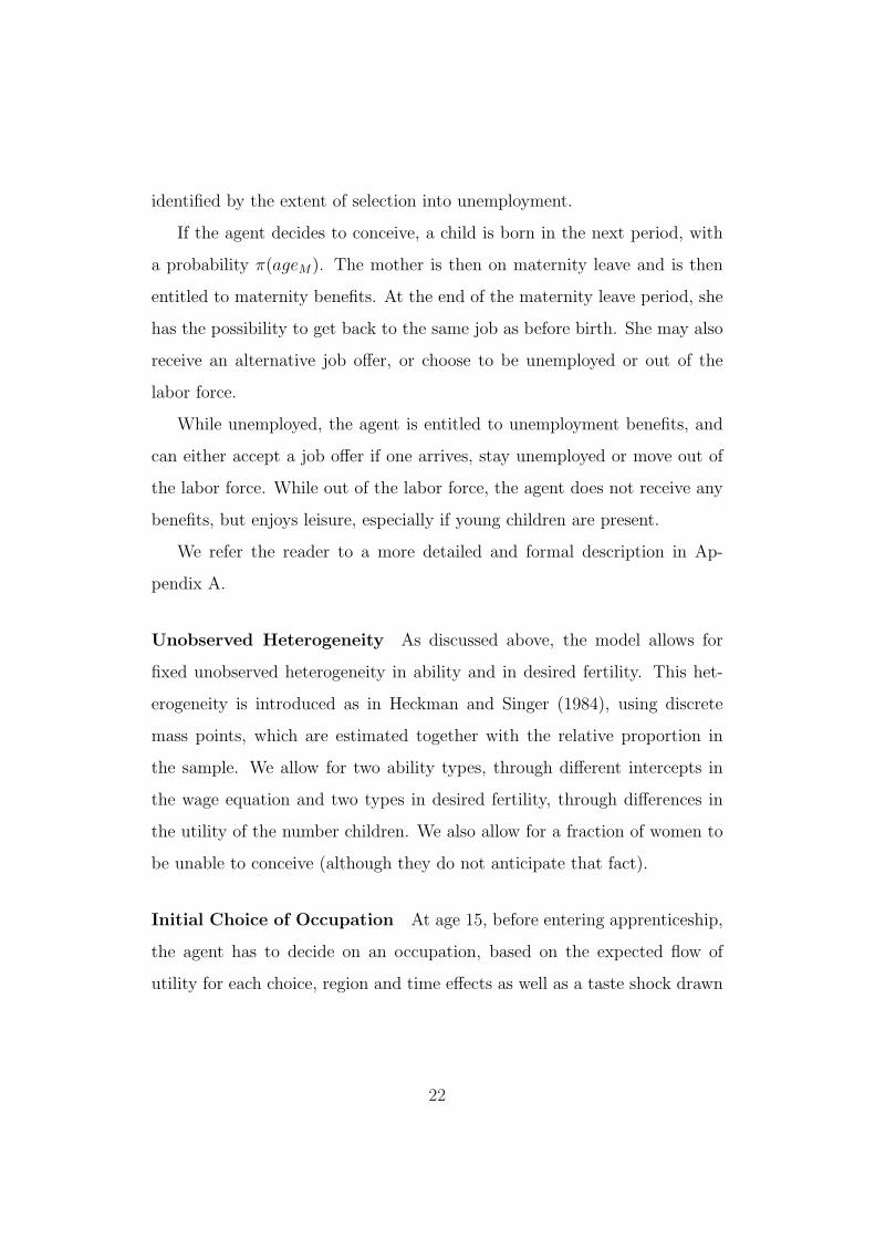
from an extreme value distribution:

maxj

[Vj + ηj]

where Vj is the intertemporal flow of utility of choosing occupation j. With

this specification, the probability of choosing a particular occupation takes

a multinomial logistic form, where the arguments are the value functions.

These value functions decompose into the sum of a current pay-off and the

future flow of utility, discounted at a rate β:

Vj = c(j, Region, T ime) + β6EWj(Ω′j)

where Wj(Ω′j) is the intertemporal flow of utility for an individual in job j,

three years later when the apprenticeship training is over. We make this

modeling assumption as in the next period the agents are eighteen years

old, and a vast majority of them are working, often in the firm that trained

them. Ω′ is the vector of state variables at age 18, with updated ages for

the female. As teenage pregnancy rates are extremely low in Germany, we

do not allow fertility decisions until that age. Second, during apprenticeship

training, unemployment is rare as all the individuals have contracts with the

training firm. 19 Hence, we do not lose much by assuming that these women

work for three years. They start making fertility and labor market decisions

once the training is over.

The current pay-off depends on the specific occupation as well as on a

set of regional dummies interacted with calendar time. Those variables will

serve as instruments for occupational choice, which is endogenous as we do

not observe the heterogenous taste for children. We discuss further the issue

of identification in the next section.

19For a more detailed discussion of the German apprenticeship system, we refer the

reader to Adda, Dustmann, Meghir, and Robin (2006).

23

4 Estimation

4.1 Methodology and Identification

The model is estimated using simulated method of moments. This allows

to combine different data sources which give information on career choices,

wages and fertility decision over the life time.

For a given set of parameters, the model is solved by backward induction

(value function iterations). The model is then simulated for agents between

age eighteen and eighty. At age fifteen, each agent decides on an occupation,

conditional on the discounted future utility and from region and time specific

costs of training. The simulated data provides a panel data set which is used

to construct moments which are compared with the moments from the real

data.

The model is identified through a judicious choice of moments. The mo-

ments we use are listed in Table 4. We first use as moments simple means of

outcome variables such as occupation, average wage by occupation, hours of

work or the number of children at different ages (usually at age 15, 20, 25,

30, 35 and 40). These moments help to make sure the model reproduces the

basic trends (and levels) in the real data. Next, we also use transition rates

from one period to another. We focus on the transition from one occupation

to another and from different choices of hours of work. These moments help

to identify the probability of receiving an offer, φi,j as well as the variance

of the taste shock for each occupational choice. Focusing on simple means is

not enough to properly identify the model, just as marginal distributions of

variables are not enough to recover their joint distribution. Therefore, we use

moments which are informative of the link between several outcomes such as

wages, fertility, occupation and work experience. We use OLS regression co-

24

efficients to capture the relationship between a number of outcome variables.

This method - also called indirect inference- was introduced by Gourieroux,

Monfort, and Renault (1993). For instance, we use the coefficients of a re-

gression of log wage on experience and experience squared by occupation as

moments to be matched by the model. We run the same regression using

simulated data and compare the coefficients from this auxiliary equation as

moments. The regression of log wage on experience helps to identify the true

return to human capital by occupation in equation (2). Similarly, to identify

the true atrophy rates in equation (1), we use a regression of the change in

(log) wages for individuals who interrupt their career on the duration of the

interruption, dummies for experience levels and the interaction of duration

and experience. 20 To link wages, the number of children and the choice of

occupation, we use coefficients from an OLS regression of log wage on age,

age squared, dummies for the number of children, occupational dummies

and the interaction between the number of children and occupational choice.

This helps to identify the coefficients in the model which pertain to fertility

(utility of children), to the dynamic trade off between children and expe-

rience (atrophy rates, return to experience) and to the interaction between

occupation and fertility in the utility function.

Finally, we use an instrumental variable approach to identify the selection

into different occupations. 21 Changes in the local demand for apprentices by

firms over time provides such exogenous variation. We use time and region

interactions at the time of initial choice of occupation (around age 15) as

20Note that these set of OLS regressions do not identify the true atrophy rates neither

in the data nor in the simulated data. Selection into different occupations, differences

in hours of work and the timing of children would bias the OLS estimates in both data

samples. However, the estimation of the structural model yields consistent estimates.21Adda, Dustmann, Meghir, and Robin (2006) use a similar identification strategy.

25

an instrument. Table 1 displays the Wald test for the joint significance of

the instrument for the first stage. The first column indicates that time and

region interactions are indeed a significant predictor of occupation at the

start of apprenticeship. Columns 2 and 3 indicate that these variables are

also significant predictors of occupational choice later on, after five and even

10 years.

The model is solved numerically using value function iterations. The

estimation is performed using the NAG e04ucf minimization routine as well

as the simplex algorithm.

4.2 Goodness of Fit

Tables 5 to 12 provide the fit of the model along different dimensions.

Table 5 displays the occupational choices overall and at the initial period

(labelled age 15). The initial and the overall proportion of women in each

occupation are rather well fitted. Table 6 displays the annual transition rate

between occupations. Persistence within the occupational choice is closely

fitted in all occupations.

Table 7 shows the proportion of females in full time, part time work,

unemployment and out of the labor force by age. The simulated proportions

of females in full time work and not working after age 20 correspond well

to the observed proportions. Part time work becomes more popular with

age both in the observed and simulated data, and the reverse holds for full

time work. Also the peak in the proportion of females out of the labor force

at age 35 is matched. The annual transition rates in hours of work in each

of the occupations is displayed in table 8. The simulated data exhibit high

persistence in each of the hours of work groups, as in the observed data. Also

the relative ranking of occupations in terms of persistence in both full time

26

and part time work is retained.

The wage-experience profile in each of the occupations is presented in

table 9. The simulated profile corresponds fairly closely to the observed

profile. Manual and abstract occupations have returns to experience which

are similar in both observed and similated data, especially at low levels of

experience.

Table 10 shows wage losses at return to work after interruptions. Longer

breaks from work and also interruptions later in the career imply larger wage

losses in both observed and simulated data. We match relatively large wage

losses in abstract occupations throughout the career, rather than in the later

career only as in the observed data. Moreover, a change in hours of work

at return to employment brings about a wage adjustment in the simulated

careers which corresponds closely to the observed change.

The profile of number of children by age is pretty well fitted in the sim-

ulated data (table 11). Females start childbearing at the same moment in

observed and simulated data. Also the timing of a second child is fairly well

fitted. Nevertheless, a slightly larger fraction of simulated females either

remains childless or gets more than one child.

The link between wages, number of children and occupation is presented

in table 12. The reference occupation is routine jobs. The simulated data

match a concave profile over age and exhibit a ’child penalty’ which is in-

creasing in the number of children, as in the observed data. Also part time

wages are fairly well matched.

4.3 Parameters

Tables 13 to 16 displays the estimated parameters together with standard

errors. In total, the model contains 161 parameters. This is rather parsi-

27

monious considering that we model five broad outcomes: wages, hours of

work, occupational choice (three categories), number of children and spacing

of each birth.

The first three rows of Table 13 display the parameters of the (log) wage

as a function of experience. Compared to the OLS coefficients displayed

in Table 9, the model implies a steeper wage profile. The average return

to experience is highest in abstract jobs. The last three rows display the

atrophy rates, i.e. the loss of human capital due to an interruption from

work for one year. The stock of experience depreciates at a lower pace early

in the career, in all occupations. Manual occupations nevertheless exhibit

the lowest depreciation rate of skill at any level of experience.

Table 14 displays the parameters pertaining to utility of work and occu-

pational choice. We allow the utility function to vary by occupation (Routine

is the default occupation), which enables to fit occupational choices over and

above initial conditions and disparities in wage profiles.

Table 15 displays the estimated offers for occupation and part time-full

time positions, conditional on previous status. Not surprisingly, the numbers

on the diagonal are larger, indicating that women are likely to keep their

occupation and hours of work for a number of periods.

Table 16 displays the parameters pertaining to unobserved heterogeneity.

We allow for four types of women, differing in terms of ability and preference

for children. Women of Type 1 and 2 are more able, with an intercept in

the log wage equation higher by about 0.128. Women of Type 1 and 3

value children more. The first row displays the estimated proportions for

each type. Types 4 and 2 (high taste for children, respectively high and low

ability) are most common, while Type 1 (low ability, low taste for children)

is least common.

28

4.4 Evidence of Selection

5 The Career Cost of Fertility

5.1 Net Present Value Calculation of Fertility Costs

In this section, we quantify the cost of children in terms of career. We

do this by simulating the model under the estimated parameterization (the

”baseline”), and simulating the model setting the probability of conception

to zero. In this counterfactual simulation, the agent knows ex ante that no

children will ever be born. This affects the choice of job at age 15, and the

subsequent career. Figures 7 and 8 plot the average path for labor supply

and wages. The proportion of women working under the baseline drops to a

low around age 33, a period when one or several children are present. As the

children are aging, the proportion of women working picks up a little again,

before starting a slow downward trend from age 42 onwards. In contrast, with

no fertility, the proportion of women working remains above 90% before age

35, after which it starts falling slowly towards 77% by age 55. Figure 8

plots the deviation of wages from the baseline with fertility. The difference

is minimal at a young age, but rises to 22% at age 37. This figure does not

give the total cost of children, as it is computed using wages, conditional on

working and it thus suffers from selection bias.

Figure 9, plots the deviation in wages by initial occupation. The highest

deviation is for women in ”routine” jobs. Interestingly, the effects peak at

different ages for the three occupational groups. The ”abstract” occupation

has a later peak which reflects the delayed fertility of this group. Figure 10

displays the differences in occupational choice at age 15. Without children,

women are more likely to go to ”abstract” jobs, which are better paid but

29

less convenient with children. About 4% more women take up these jobs,

coming almost equally from ”routine” and ”manual” jobs.

Table 17 computes the cost of children by calculating the net present

value of children in terms of earnings, at age 15. We evaluate this statistic

by simulating the careers of women twice, allowing fertility and putting it to

zero. The cost of children then reflects the difference in net present value of

the lifetime earnings, unemployment benefits and maternity leave compen-

sations evaluated at age 15. We use an annual discount factor of 0.95 in the

calculation. The first line of the table computes the average treatment effect

(ATE). This is obtained by averaging both streams of income (including un-

employment or maternity benefits) for all individuals. We evaluate the ATE

at 125%, i.e. without fertility the lifetime income stream is 125% higher. We

also calculate the cost of children by initial occupation. The cost is highest

for women in ”routine” occupations and lowest for those in ”abstract” jobs.

Part of these differences reflect the higher fertility rates in ”routine” jobs and

lower ones in ”abstract” occupations.

The next line of Table 17 presents the average treatment on the treated

(ATT), using only those who have children in the baseline simulation. This

figure is higher, at 142%. This implies that women who select themselves into

motherhood actually bear a higher career cost of children. Compared to the

ATE, the cost rises more for women in ”abstract” jobs, so that the differences

in cost across occupation is reduced, when conditioning on mothers.

The large career costs due to children does not mean that having children

is not an irrational choice. The next line of Table 17 displays the total welfare

cost of denying fertility. Those are clearly negative, with a loss of 17% in

welfare. Again, the loss is highest in occupations where fertility is the highest.

We next decompose the ATE into various components to understand the

30

sources of the costs of children. There are several channels that affects these

costs. First, due to career interruptions, women accumulate less human

capital and have therefore lower wages than they would have had without

children. Second, mothers are more likely to take up part-time jobs or even

to drop out of the labor force, so another channel are un-earned wages.

Third, future fertility may induce a selection into occupations for which skill

depreciation is lower, with flatter income profiles but with lower wages.

We first evaluate the importance of wages. We compare the baseline ca-

reers (with fertility) with the careers women would have had without children,

but we give them the wage without children whenever they work. Hence, in

this decomposition, the wage component of the cost is gone. We find a cost

which is substantially lower, at about 23%.

Next, we simulate an economy where we impose on mothers the labor

supply they would have chosen without children. 22 The cost of children is

in this case more substantial at about 50%. This implies that a large part of

the career cost can be attributed to forgone wages during interruptions from

work. The third channel is selection of occupation. Here again, we impose on

mothers the occupation they would have chosen without children. As shown

in Figure 10, without children, women are more likely to go into ”abstract”

jobs in which wages are higher. Hence, one would expect a positive cost of

having children. In fact, the effect is more complex. ”Abstract” jobs are also

more difficult to manage with children, and mothers in those occupations are

more likely to drop out of the labor market or go part-time. Hence mothers

who are ”forced” into those occupations are at a disadvantage. The overall

effect is in fact negative, although small at around 1%.

22Note that in these simulations, the agents do not anticipate that their labor supply or

wages will be different.

31

Note that as the model is non-linear, the decompositions do not sum to

the total ATE displayed in the first line of Table 17.

The table then decomposes further the labor supply and the wage effect.

We simulate out baseline mothers in an environment where there is no atro-

phy of human capital. Mothers thus do not lose skills when dropping out of

work. These results, however, indicate that depreciation of skills represents

only a small career cost (19.8%). This cost is higher in abstract occupations

since atrophy rates are high, especially later in the career, and females in

this occupation start childbearing later. The next row of table 17 looks into

the hours of work. It assigns mothers the hours of work as if they had no

children, conditional on working. In this case, mothers work a lot more full

time instead of part time, and this implies a career cost of 21.7%. In the

last row, mothers’ careers are simulated where they are assigned the stock of

human capital of the no-fertility situation. This reflects part of the wage cost

of fertility by keeping the stock of human capital at the level of non-mothers.

This entails a cost of 37.8% and indicates that the depreciation and the lack

of human capital accumulation for mothers is an important factor in the total

career cost.

Finally, we evaluate the cost of just one child. Women are fertile for up

to one child only. The career cost is then equal to a 44% in net present

value. This is less than half of the overall cost, which suggests that there

are non-linearities in the cost of children. Two children are more costly as

women are more likely to drop out of the labor market.

Overall, these results suggest that forgone wages during interruptions of

work are a main factor driving the career cost of fertility, combined with the

loss and non-accumulation of human capital during interruptions.

32

5.2 Fertility and the Gender Wage Gap

We evaluate in this section the extent to which the gender wage gap can be

explained by realized and future fertility patterns.

5.3 How are Pro-Fertility Policies Affecting the Ca-

reers of Women?

In many countries, the tax system encourages fertility. This is also the case

in Germany, where parents receive monetary compensations from the gov-

ernment when they get children. Our goal in this section is two-fold. First,

we evaluate how fertility responds to monetary incentives and benchmark

the results with other studies which have used different methodology and

identification strategies. Second, we evaluate the effect of these policies on

the careers of women, and in particular on the gender wage gap.

Several papers have analyzed the elasticity of fertility with respect to

income or government transfers. For instance XXX... uses.

6 Conclusion

This paper aims to understand the way women make career choices jointly

with fertility choices. In particular we analyse the timing of the first child

as well as subsequent fertility decisions, and how these interact with, deter-

mine, and are determined by occupational choice. The paper makes three

contributions; first, it develops a model of fertility and career choice over the

life-cycle. Second, it uses unique data that contains information allowing a

much more general approach to this question than previous papers. Third,

the analysis is for a country where the educational system locks individu-

33

als into a particular occupation before the fertility period (Germany). This

avoids problems with unraveling the timing of the two choices, and provides

instruments for occupational choice in form of regional occupation structure.

It enables us to disentangle occupational choices and fertility decisions.

Our empirical analysis is based on a combination of two data sets which

provide detailed information on wage progression, labor market participation,

occupational choice and fertility over the life-cycle. We find that raising

children accounts for about 125% loss in lifetime income. This decrease is

due to three different factors: forgone wages during interruptions from work,

the lack of accumulation and loss of human capital due to interrupted careers,

and the sorting of mothers into child-friendly occupations. Our results also

emphasize the role of the wage profile in shaping fertility and the timing of

births. Our estimated model shows that interruptions in careers lead to a loss

of human capital which is larger for women with higher work experience and

differs across occupation. This differential loss explains partly the fertility

patterns across occupations. Similarly, the return to experience also shapes

fertility.

34

References

Adda, J., C. Dustmann, C. Meghir, and J.-M. Robin (2006): “Career Progressionand Formal versus on the Job Training,” IZA Discussion Paper No. 2260.

Albrecht, J., P.-A. Edin, M. Sundstrom, and S. Vroman (1999): “Career Inter-ruptions and Subsequent Earnings: A Reexamination Using Swedish Data,” Journal ofHuman Resources, 34, 294–312.

Altug, S., and R. A. Miller (1998): “The Effect of Work Experience on Female Wageand Labor Supply,” Review of Economic Studies, 65(1), 45–85.

Arroyo, C. R., and J. Z. J (1997): “Dynamic Microeconomic Models Of FertilityChoice: A Survey,” Journal of Population Economics, 10, 23–65.

Attanasio, O., H. Low, and V. Sanchez-Marcos (2004): “Explaining Changes inFemale Labour Supply in a Life-cycle Model,” University of Cambridge Working Paper04/51.

Autor, D. H., F. Levy, and R. J. Murnane (2003): “The Skill Content of RecentTechnological Change: An empirical exploration*,” Quarterly Journal of Economics,118(4), 1279–1333.

Becker, G. (1960): “An Economic Analysis Of Fertility,” in Demography And EconomicChange In Developed Countries, pp. 209–231. Universities-NBER Research ConferenceSeries 11, Princeton.

Becker, G., and H. G. Lewis (1973): “On the Interaction between the Quantity andQuality of Children,” The Journal of Political Economy, 81(2), S279–S288.

Bender, S., A. Haas, and C. Klose (2000): “IAB Employment Subsample 1975-1995:Opportunities for Analysis provided by the Anonymised Subsample,” Discussion Paper117, IZA, Bonn.

Black, S. E., and A. Spitz-Oener (2010): “Explaining Women’s Success: Techno-logical Change and the Skill Content of Women’s Work,” Review of Economics andStatistics, 92(1), 187–194.

Brown, R. S., M. Moon, and B. S. Zoloth (1980): “Occupational Attainment AndSegregation By Sex,” Industrial and Labor Relations Review, 33(4), 506–517.

Carrington, W. J., and K. R. Troske (1995): “Gender Segregation In Small Firms,”The Journal of Human Resources, 30(3), 503–533.

Cigno, A., and J. Ermisch (1989): “A Microeconomic Analysis Of The Timing OfBirths,” European Economic Review, 33, 737–760.

Eckstein, Z., and K. I. Wolpin (1989): “Dynamic Labour Force Participation ofMarried Women and Endogenous Wage Growth,” Review of Economic Studies, 56(3),375–390.

35

Francesconi, M. (2002): “A Joint Dynamic Model of Fertility and Work of MarriedWomen,” Journal of Labor Economics, 20, 336–380.

Gathmann, C., and U. Schonberg (2010): “How General Is Human Capital? ATask-Based Approach,” Journal of Labor Economics, 28(1), 1–49.

Goldin, C., and L. Katz (2002): “The Power of the Pill: Oral Contraceptives andWomen’s Career and Marriage Decisions,” Journal of Political Economy, 110(4), 730–770.

Gourieroux, C., A. Monfort, and E. Renault (1993): “Indirect Inference,” Journalof Applied Econometrics, 8, S85–S118.

Gronau, R. (1988): “Sex-Related Wage Differentials and Women’s Interrupted LaborCareers- the Chicken or the Egg,” Journal of Labor Economics, 6(3), 277–301.

Groshen, E. L. (1991): “The Structure Of The Female/Male Wage Differential: Is ItWho You Are, What You Do, Or Where You Work?,” The Journal of Human Resources,26(3), 457–472.

Haisken-DeNew, J. P., and J. R. Frick (2003): “Desktop Companion to the GermanSocio-Economic Panel Study (SOEP),” DIW, Berlin.

Heckman, J., and B. Singer (1984): “A Method for Minimizing the Impact of Distri-butional Assumptions in Econometric Models for Duration Data,” Econometrica, 52(2),271–320.

Heckman, J. J., and T. E. Macurdy (1980): “A Life Cycle Model of Female LabourSupply,” Review of Economic Studies, 47(1), 47–74.

Heckman, J. J., and J. R. Walker (1990): “The Relationship Between Wages andIncome and the Timing and Spacing of Births: Evidence from Swedish LongitudinalData,” Econometrica, 58(6), 1411–1441.

Hotz, J., and R. Miller (1988): “An Empirical Analysis of Life Cycle Fertility andFemale Labor Supply,” Econometrica, 56(1), 91–118.

Keane, M., and K. Wolpin (2006): “The Role of Labor and Marriage Markets, Pref-erence Heterogeneity and the Welfare System in the Life Cycle Decisions of Black,Hispanic and White Women,” Pier Working Paper 06-004.

(2007): “Exploring the Usefulness of a Nonrandom Holdout Sample for Model Val-idation: Welfare Effects on Female Behavior,” International Economic Review, 48(4),1351–1378.

Keane, M. P., and K. I. Wolpin (1997): “The Career Decisions of Young Men,”Journal of Political Economy, 105(3), 473–522.

Miller, A. (2008): “The Effects of Motherhood Timing on Career Path,” mimeo, Uni-versity of Virginia.

36

Mincer, J., and H. Olfek (1982): “Interrupted Work Careers: Depreciation andRestoration of Human Capital,” Journal of Human Resources, 17, 3–24.

Mincer, J., and S. Polachek (1974): “Family Investments in Human Capital: Earn-ings of Women,” Journal of Political Economy, 82(2), S76–S108.

Moffitt, R. (1984): “Profiles of Fertility, Labour Supply and Wages of Married Women:A Complete Life-Cycle Model,” Review of Economic Studies, 51(2), 263–278.

Newman, J., and C. McCulloch (1984): “A Hazard Rate Approach To The TimingOf Births,” Econometrica, 52, 939–962.

Polachek, S. (1981): “Occupational Self-Selection: A Human Capital Approach ToSex Differences In Occupational Structure,” Review of Economics and Statistics, 63(1),60–69.

Rosenzweig, M., and P. Schultz (1985): “The Demand For And Supply Of Births:Fertility And Its Life Cycle Consequences,” American Economic Review, 75(5), 992–1015.

van der Klaauw, W. (1996): “Female Labor Supply and Marital Status Decisions: ALife-Cycle Model,” Review of Economic Studies, 63(2), 199–235.

Weiss, Y., and R. Gronau (1981): “Expected Interruptions in Labor Force Partici-pation and Sex-Related Differences in Earnings Growth,” Review of Economic Studies,48.

Wolpin, K. I. (1984): “An Estimable Dynamic Stochastic Model of Fertility and ChildMortality,” Journal of Political Economy, 92(5), 852–874.

37

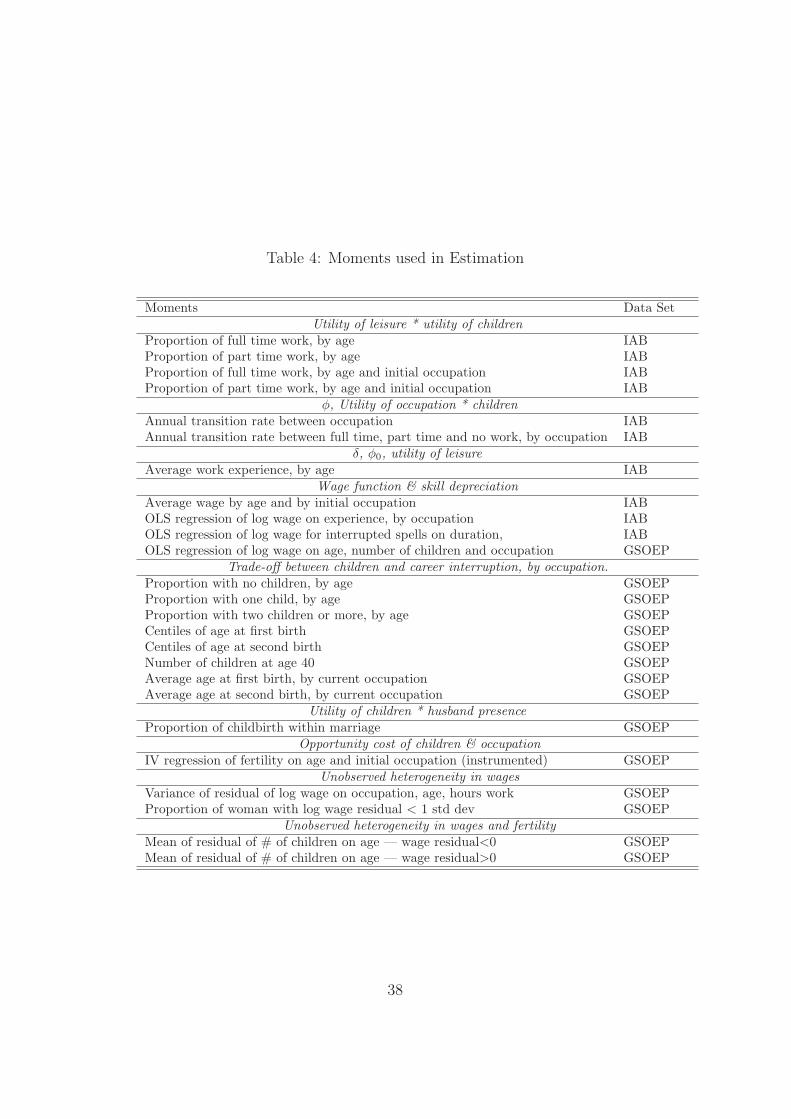
Table 4: Moments used in Estimation

Moments Data SetUtility of leisure * utility of children

Proportion of full time work, by age IABProportion of part time work, by age IABProportion of full time work, by age and initial occupation IABProportion of part time work, by age and initial occupation IAB

φ, Utility of occupation * childrenAnnual transition rate between occupation IABAnnual transition rate between full time, part time and no work, by occupation IAB

δ, φ0, utility of leisureAverage work experience, by age IAB

Wage function & skill depreciationAverage wage by age and by initial occupation IABOLS regression of log wage on experience, by occupation IABOLS regression of log wage for interrupted spells on duration, IABOLS regression of log wage on age, number of children and occupation GSOEP

Trade-off between children and career interruption, by occupation.Proportion with no children, by age GSOEPProportion with one child, by age GSOEPProportion with two children or more, by age GSOEPCentiles of age at first birth GSOEPCentiles of age at second birth GSOEPNumber of children at age 40 GSOEPAverage age at first birth, by current occupation GSOEPAverage age at second birth, by current occupation GSOEP

Utility of children * husband presenceProportion of childbirth within marriage GSOEP

Opportunity cost of children & occupationIV regression of fertility on age and initial occupation (instrumented) GSOEP

Unobserved heterogeneity in wagesVariance of residual of log wage on occupation, age, hours work GSOEPProportion of woman with log wage residual < 1 std dev GSOEP

Unobserved heterogeneity in wages and fertilityMean of residual of # of children on age — wage residual<0 GSOEPMean of residual of # of children on age — wage residual>0 GSOEP

38

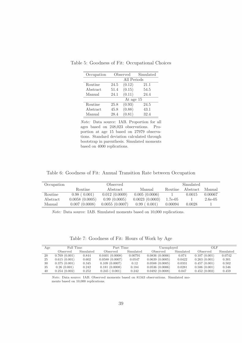
Table 5: Goodness of Fit: Occupational Choices

Occupation Observed SimulatedAll Periods

Routine 24.5 (0.12) 21.1Abstract 51.4 (0.15) 54.5Manual 24.1 (0.11) 24.4

At age 15Routine 25.8 (0.93) 24.5Abstract 45.8 (0.88) 43.1Manual 28.4 (0.81) 32.4

Note: Data source: IAB. Proportion for allages based on 248,023 observations. Pro-portion at age 15 based on 27979 observa-tions. Standard deviation calculated throughbootstrap in parenthesis. Simulated momentsbased on 4000 replications.

Table 6: Goodness of Fit: Annual Transition Rate between Occupation

Occupation Observed SimulatedRoutine Abstract Manual Routine Abstract Manual

Routine 0.98 ( 0.001) 0.012 (0.0009) 0.005 (0.0006) 1 0.0015 0.00067Abstract 0.0058 (0.0005) 0.99 (0.0005) 0.0023 (0.0003) 1.7e-05 1 2.6e-05Manual 0.007 (0.0008) 0.0055 (0.0007) 0.99 ( 0.001) 0.00094 0.0028 1

Note: Data source: IAB. Simulated moments based on 10,000 replications.

Table 7: Goodness of Fit: Hours of Work by Age

Age Full Time Part Time Unemployed OLFObserved Simulated Observed Simulated Observed Simulated Observed Simulated

20 0.769 (0.001) 0.844 0.0401 (0.0008) 0.00791 0.0836 (0.0006) 0.074 0.107 (0.001) 0.074225 0.615 (0.001) 0.602 0.0588 (0.0007) 0.0547 0.0639 (0.0005) 0.0422 0.263 (0.001) 0.30130 0.375 (0.001) 0.345 0.109 (0.0007) 0.12 0.0588 (0.0005) 0.0331 0.457 (0.001) 0.50235 0.26 (0.001) 0.242 0.181 (0.0008) 0.184 0.0536 (0.0006) 0.0281 0.506 (0.001) 0.54640 0.254 (0.002) 0.252 0.245 ( 0.001) 0.242 0.0492 (0.0008) 0.047 0.452 (0.002) 0.459

Note: Data source: IAB. Observed moments based on 81343 observations. Simulated mo-ments based on 10,000 replications.

39

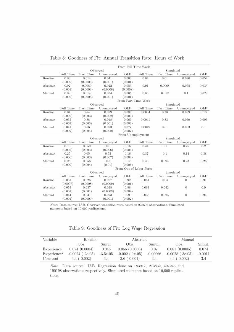
Table 8: Goodness of Fit: Annual Transition Rate: Hours of Work

From Full Time WorkObserved Simulated

Full Time Part Time Unemployed OLF Full Time Part Time Unemployed OLFRoutine 0.88 0.014 0.041 0.068 0.84 0.01 0.096 0.054

(0.002) (0.0006) (0.001) (0.001)Abstract 0.92 0.0089 0.022 0.053 0.91 0.0068 0.055 0.033

(0.001) (0.0003) (0.0006) (0.0008)Manual 0.89 0.014 0.034 0.065 0.86 0.012 0.1 0.029

(0.002) (0.0006) (0.001) (0.001)From Part Time Work

Observed SimulatedFull Time Part Time Unemployed OLF Full Time Part Time Unemployed OLF

Routine 0.04 0.84 0.029 0.089 0.0034 0.78 0.089 0.13(0.002) (0.003) (0.002) (0.003)

Abstract 0.035 0.88 0.018 0.069 0.0041 0.83 0.069 0.093(0.002) (0.003) (0.001) (0.002)

Manual 0.041 0.86 0.023 0.077 0.0049 0.81 0.083 0.1(0.002) (0.004) (0.002) (0.002)

From UnemploymentObserved Simulated

Full Time Part Time Unemployed OLF Full Time Part Time Unemployed OLFRoutine 0.18 0.059 0.6 0.16 0.44 0.1 0.25 0.2

(0.005) (0.003) (0.006) (0.004)Abstract 0.25 0.05 0.53 0.16 0.37 0.1 0.14 0.38

(0.006) (0.003) (0.007) (0.004)Manual 0.28 0.056 0.5 0.17 0.43 0.094 0.23 0.25

(0.009) (0.004) (0.01) (0.006)From Out of Labor Force

Observed SimulatedFull Time Part Time Unemployed OLF Full Time Part Time Unemployed OLF

Routine 0.031 0.026 0.027 0.92 0.051 0.04 0 0.91(0.0007) (0.0008) (0.0009) (0.001)

Abstract 0.053 0.037 0.028 0.88 0.061 0.042 0 0.9(0.001) (0.001) (0.0009) (0.002)

Manual 0.044 0.031 0.023 0.9 0.038 0.025 0 0.94(0.001) (0.0009) (0.001) (0.002)

Note: Data source: IAB. Observed transition rates based on 925602 observations. Simulatedmoments based on 10,000 replications.

Table 9: Goodness of Fit: Log Wage Regression

Variable Routine Abstract ManualObs. Simul. Obs. Simul. Obs. Simul.

Experience 0.074 (0.0004) 0.045 0.066 (0.0003) 0.07 0.081 (0.0005) 0.074Experience2 -0.0024 ( 2e-05) -3.5e-05 -0.002 ( 1e-05) -0.00066 -0.0028 ( 3e-05) -0.0011Constant 3.4 ( 0.002) 3.4 3.6 ( 0.001) 3.4 3.4 ( 0.002) 3.4

Note: Data source: IAB. Regression done on 183917, 213832, 497245 and190198 observations respectively. Simulated moments based on 10,000 replica-tions.

40

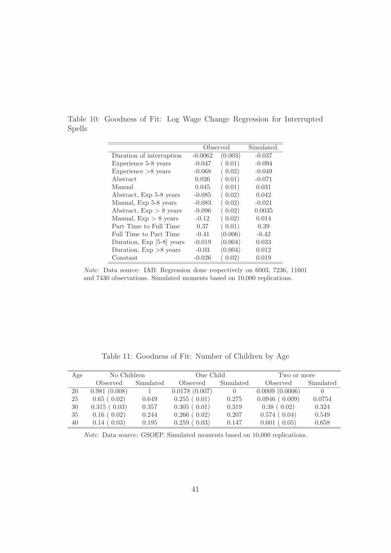
Table 10: Goodness of Fit: Log Wage Change Regression for InterruptedSpells

Observed Simulated.Duration of interruption -0.0062 (0.003) -0.037Experience 5-8 years -0.047 ( 0.01) -0.094Experience >8 years -0.068 ( 0.02) -0.049Abstract 0.026 ( 0.01) -0.071Manual 0.045 ( 0.01) 0.031Abstract, Exp 5-8 years -0.085 ( 0.02) 0.042Manual, Exp 5-8 years -0.083 ( 0.02) -0.021Abstract, Exp > 8 years -0.096 ( 0.02) 0.0035Manual, Exp > 8 years -0.12 ( 0.02) 0.014Part Time to Full Time 0.37 ( 0.01) 0.39Full Time to Part Time -0.41 (0.006) -0.42Duration, Exp [5-8] years -0.019 (0.004) 0.033Duration, Exp >8 years -0.03 (0.004) 0.012Constant -0.026 ( 0.02) 0.019

Note: Data source: IAB: Regression done respectively on 6003, 7236, 11601and 7430 observations. Simulated moments based on 10,000 replications.

Table 11: Goodness of Fit: Number of Children by Age

Age No Children One Child Two or moreObserved Simulated Observed Simulated Observed Simulated

20 0.981 (0.008) 1 0.0178 (0.007) 0 0.0009 (0.0006) 025 0.65 ( 0.02) 0.649 0.255 ( 0.01) 0.275 0.0946 ( 0.009) 0.075430 0.315 ( 0.03) 0.357 0.305 ( 0.01) 0.319 0.38 ( 0.02) 0.32435 0.16 ( 0.02) 0.244 0.266 ( 0.02) 0.207 0.574 ( 0.04) 0.54940 0.14 ( 0.03) 0.195 0.259 ( 0.03) 0.147 0.601 ( 0.05) 0.658

Note: Data source: GSOEP. Simulated moments based on 10,000 replications.

41

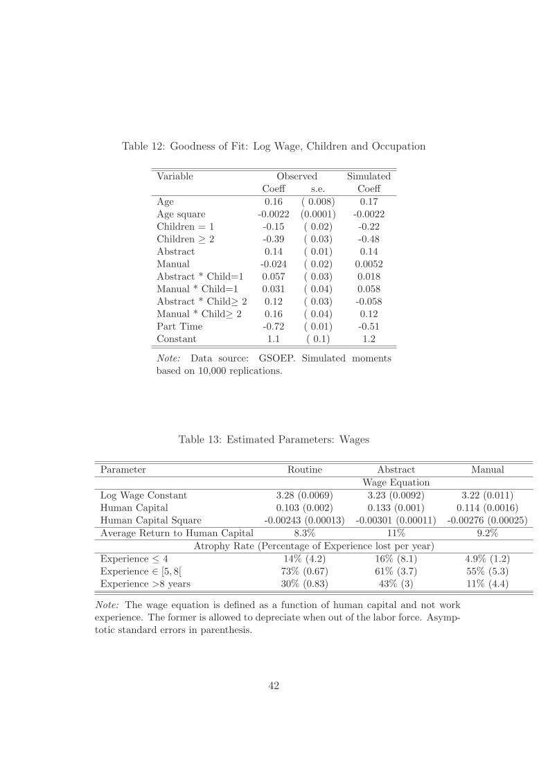
Table 12: Goodness of Fit: Log Wage, Children and Occupation

Variable Observed SimulatedCoeff s.e. Coeff

Age 0.16 ( 0.008) 0.17Age square -0.0022 (0.0001) -0.0022Children = 1 -0.15 ( 0.02) -0.22Children ≥ 2 -0.39 ( 0.03) -0.48Abstract 0.14 ( 0.01) 0.14Manual -0.024 ( 0.02) 0.0052Abstract * Child=1 0.057 ( 0.03) 0.018Manual * Child=1 0.031 ( 0.04) 0.058Abstract * Child≥ 2 0.12 ( 0.03) -0.058Manual * Child≥ 2 0.16 ( 0.04) 0.12Part Time -0.72 ( 0.01) -0.51Constant 1.1 ( 0.1) 1.2

Note: Data source: GSOEP. Simulated momentsbased on 10,000 replications.

Table 13: Estimated Parameters: Wages

Parameter Routine Abstract ManualWage Equation

Log Wage Constant 3.28 (0.0069) 3.23 (0.0092) 3.22 (0.011)Human Capital 0.103 (0.002) 0.133 (0.001) 0.114 (0.0016)Human Capital Square -0.00243 (0.00013) -0.00301 (0.00011) -0.00276 (0.00025)Average Return to Human Capital 8.3% 11% 9.2%

Atrophy Rate (Percentage of Experience lost per year)Experience ≤ 4 14% (4.2) 16% (8.1) 4.9% (1.2)Experience ∈ [5, 8[ 73% (0.67) 61% (3.7) 55% (5.3)Experience >8 years 30% (0.83) 43% (3) 11% (4.4)

Note: The wage equation is defined as a function of human capital and not workexperience. The former is allowed to depreciate when out of the labor force. Asymp-totic standard errors in parenthesis.

42

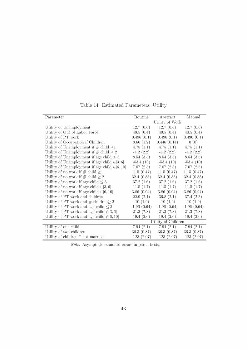
Table 14: Estimated Parameters: Utility

Parameter Routine Abstract ManualUtility of Work

Utility of Unemployment 12.7 (0.6) 12.7 (0.6) 12.7 (0.6)Utility of Out of Labor Force 40.5 (0.4) 40.5 (0.4) 40.5 (0.4)Utility of PT work 0.496 (0.1) 0.496 (0.1) 0.496 (0.1)Utility of Occupation if Children 8.66 (1.2) 0.446 (0.14) 0 (0)Utility of Unemployment if # child ≥1 4.75 (1.1) 4.75 (1.1) 4.75 (1.1)Utility of Unemployment if # child ≥ 2 -4.2 (2.2) -4.2 (2.2) -4.2 (2.2)Utility of Unemployment if age child ≤ 3 8.54 (3.5) 8.54 (3.5) 8.54 (3.5)Utility of Unemployment if age child ∈]3, 6] -53.4 (10) -53.4 (10) -53.4 (10)Utility of Unemployment if age child ∈]6, 10] 7.07 (2.5) 7.07 (2.5) 7.07 (2.5)Utility of no work if # child ≥1 11.5 (0.47) 11.5 (0.47) 11.5 (0.47)Utility of no work if # child ≥ 2 32.4 (0.83) 32.4 (0.83) 32.4 (0.83)Utility of no work if age child ≤ 3 37.2 (1.6) 37.2 (1.6) 37.2 (1.6)Utility of no work if age child ∈]3, 6] 11.5 (1.7) 11.5 (1.7) 11.5 (1.7)Utility of no work if age child ∈]6, 10] 3.86 (0.94) 3.86 (0.94) 3.86 (0.94)Utility of PT work and children 22.9 (2.1) 36.8 (2.1) 37.4 (2.3)Utility of PT work and # children≥ 2 -10 (1.9) -10 (1.9) -10 (1.9)Utility of PT work and age child ≤ 3 -1.96 (0.64) -1.96 (0.64) -1.96 (0.64)Utility of PT work and age child ∈]3, 6] 21.3 (7.8) 21.3 (7.8) 21.3 (7.8)Utility of PT work and age child ∈]6, 10] 19.4 (2.6) 19.4 (2.6) 19.4 (2.6)

Utility of ChildrenUtility of one child 7.94 (2.1) 7.94 (2.1) 7.94 (2.1)Utility of two children 36.3 (0.87) 36.3 (0.87) 36.3 (0.87)Utility of children * not married -123 (2.07) -123 (2.07) -123 (2.07)

Note: Asymptotic standard errors in parenthesis.

43

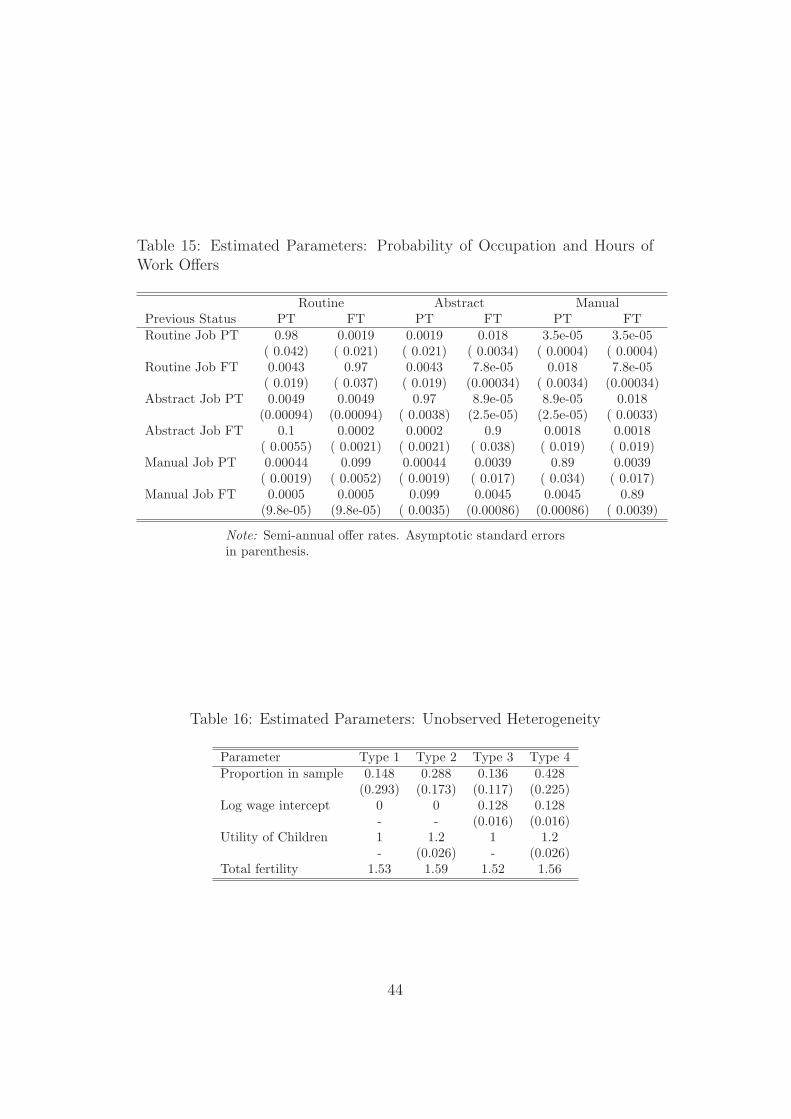
Table 15: Estimated Parameters: Probability of Occupation and Hours ofWork Offers

Routine Abstract ManualPrevious Status PT FT PT FT PT FTRoutine Job PT 0.98 0.0019 0.0019 0.018 3.5e-05 3.5e-05

( 0.042) ( 0.021) ( 0.021) ( 0.0034) ( 0.0004) ( 0.0004)Routine Job FT 0.0043 0.97 0.0043 7.8e-05 0.018 7.8e-05

( 0.019) ( 0.037) ( 0.019) (0.00034) ( 0.0034) (0.00034)Abstract Job PT 0.0049 0.0049 0.97 8.9e-05 8.9e-05 0.018

(0.00094) (0.00094) ( 0.0038) (2.5e-05) (2.5e-05) ( 0.0033)Abstract Job FT 0.1 0.0002 0.0002 0.9 0.0018 0.0018

( 0.0055) ( 0.0021) ( 0.0021) ( 0.038) ( 0.019) ( 0.019)Manual Job PT 0.00044 0.099 0.00044 0.0039 0.89 0.0039

( 0.0019) ( 0.0052) ( 0.0019) ( 0.017) ( 0.034) ( 0.017)Manual Job FT 0.0005 0.0005 0.099 0.0045 0.0045 0.89

(9.8e-05) (9.8e-05) ( 0.0035) (0.00086) (0.00086) ( 0.0039)

Note: Semi-annual offer rates. Asymptotic standard errorsin parenthesis.

Table 16: Estimated Parameters: Unobserved Heterogeneity

Parameter Type 1 Type 2 Type 3 Type 4Proportion in sample 0.148 0.288 0.136 0.428

(0.293) (0.173) (0.117) (0.225)Log wage intercept 0 0 0.128 0.128

- - (0.016) (0.016)Utility of Children 1 1.2 1 1.2

- (0.026) - (0.026)Total fertility 1.53 1.59 1.52 1.56

44

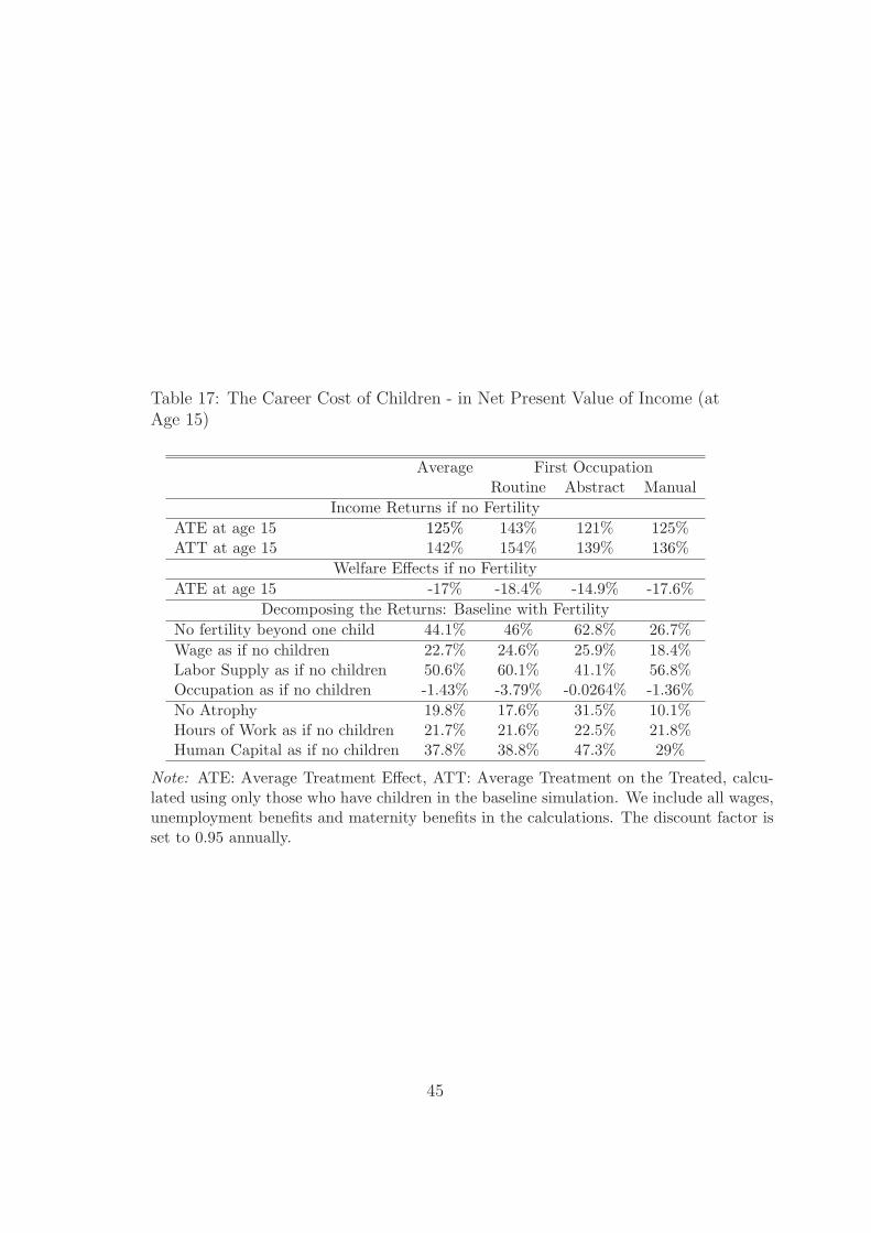
Table 17: The Career Cost of Children - in Net Present Value of Income (atAge 15)

Average First OccupationRoutine Abstract Manual

Income Returns if no FertilityATE at age 15 125% 143% 121% 125%ATT at age 15 142% 154% 139% 136%

Welfare Effects if no FertilityATE at age 15 -17% -18.4% -14.9% -17.6%

Decomposing the Returns: Baseline with FertilityNo fertility beyond one child 44.1% 46% 62.8% 26.7%Wage as if no children 22.7% 24.6% 25.9% 18.4%Labor Supply as if no children 50.6% 60.1% 41.1% 56.8%Occupation as if no children -1.43% -3.79% -0.0264% -1.36%No Atrophy 19.8% 17.6% 31.5% 10.1%Hours of Work as if no children 21.7% 21.6% 22.5% 21.8%Human Capital as if no children 37.8% 38.8% 47.3% 29%

Note: ATE: Average Treatment Effect, ATT: Average Treatment on the Treated, calcu-lated using only those who have children in the baseline simulation. We include all wages,unemployment benefits and maternity benefits in the calculations. The discount factor isset to 0.95 annually.

45

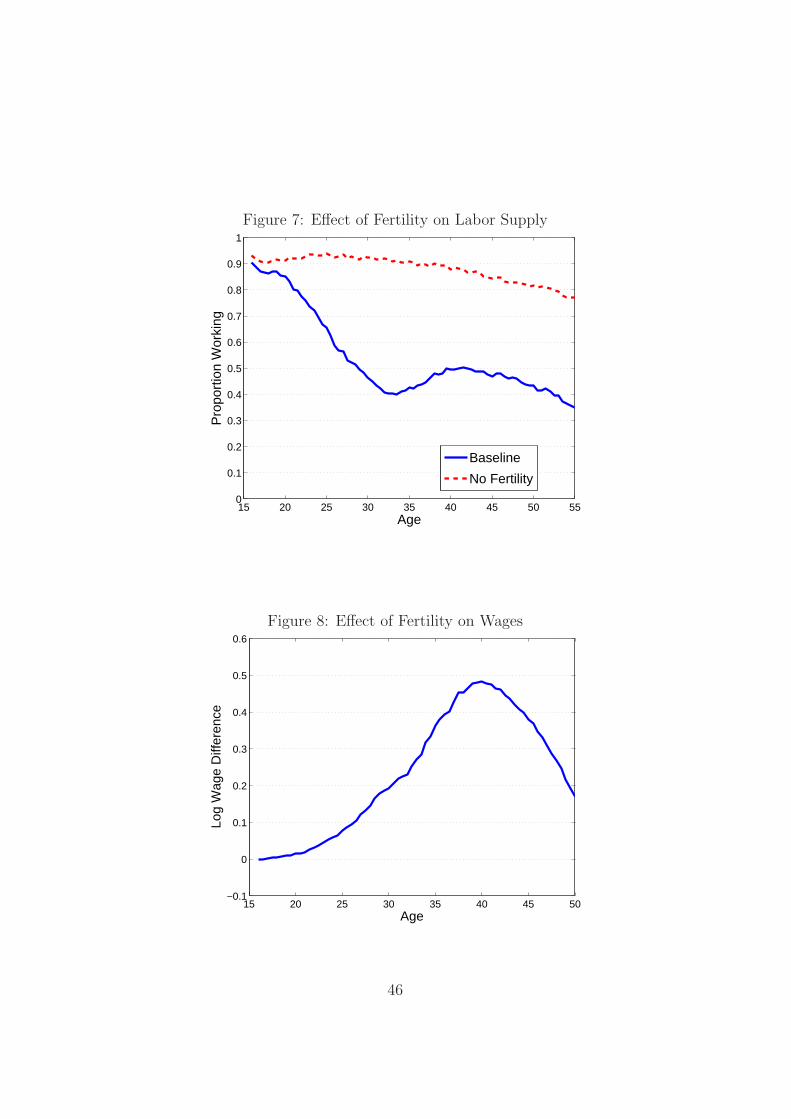
Figure 7: Effect of Fertility on Labor Supply

15 20 25 30 35 40 45 50 550

0.1

0.2

0.3

0.4

0.5

0.6

0.7

0.8

0.9

1

Age

Pro

port

ion

Wor

king

Baseline

No Fertility

Figure 8: Effect of Fertility on Wages

15 20 25 30 35 40 45 50−0.1

0

0.1

0.2

0.3

0.4

0.5

0.6

Age

Log

Wag

e D

iffer

ence

46

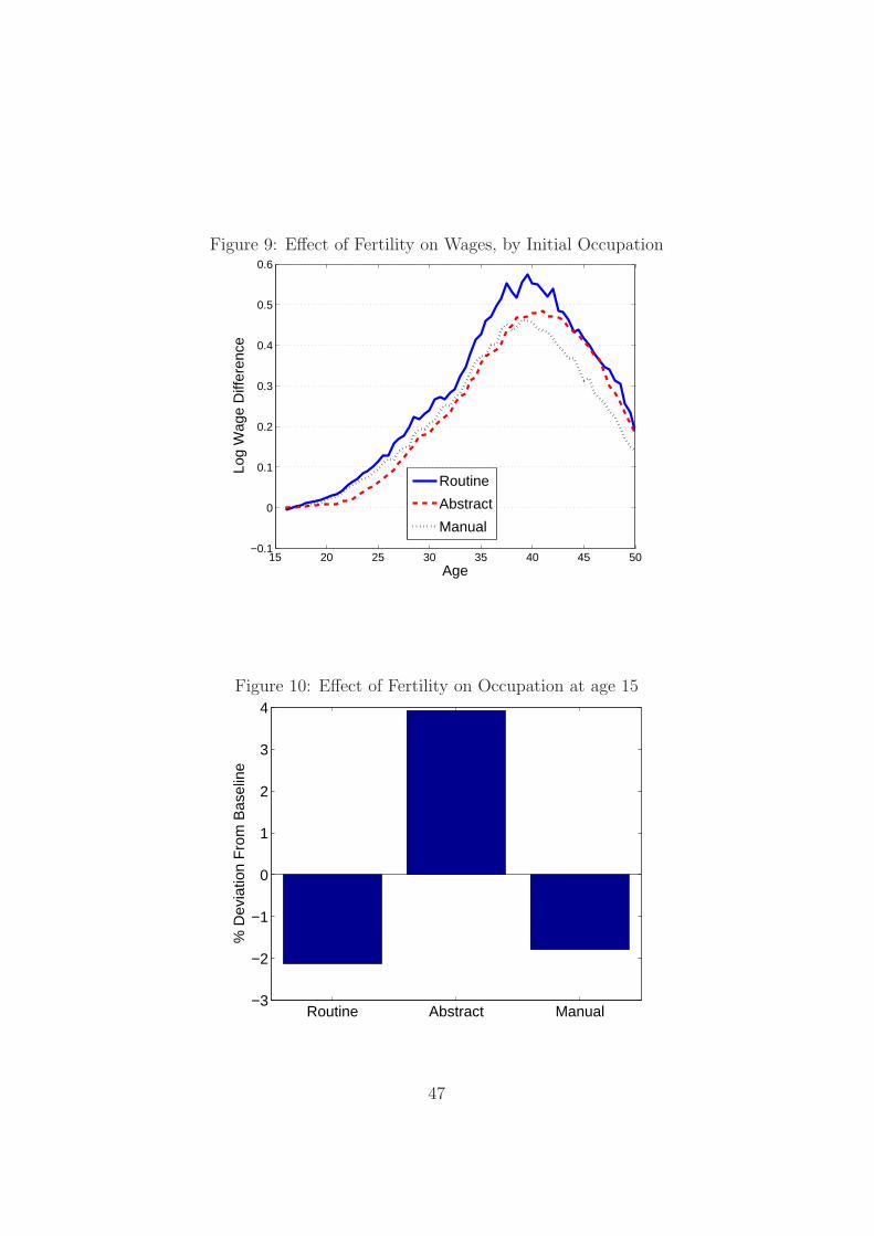
Figure 9: Effect of Fertility on Wages, by Initial Occupation

15 20 25 30 35 40 45 50−0.1

0

0.1

0.2

0.3

0.4

0.5

0.6

Age

Log

Wag

e D

iffer

ence

Routine

Abstract

Manual

Figure 10: Effect of Fertility on Occupation at age 15

Routine Abstract Manual−3

−2

−1

0

1

2

3

4

% D

evia

tion

Fro

m B

asel

ine

47

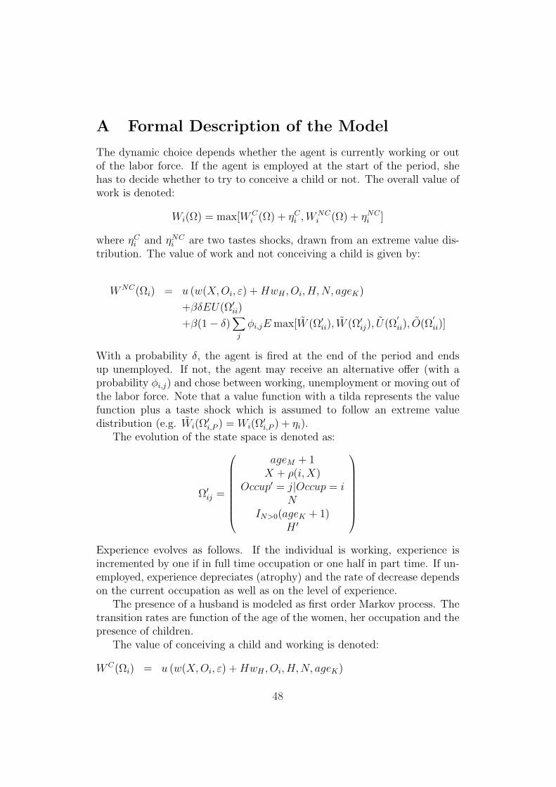
A Formal Description of the Model

The dynamic choice depends whether the agent is currently working or outof the labor force. If the agent is employed at the start of the period, shehas to decide whether to try to conceive a child or not. The overall value ofwork is denoted:

Wi(Ω) = max[WCi (Ω) + ηC

i ,WNCi (Ω) + ηNC

i ]

where ηCi and ηNC

i are two tastes shocks, drawn from an extreme value dis-tribution. The value of work and not conceiving a child is given by:

WNC(Ωi) = u (w(X,Oi, ε) + HwH , Oi, H, N, ageK)

+βδEU(Ω′ii)

+β(1− δ)∑

j

φi,jE max[W (Ω′ii), W (Ω′

ij), U(Ω′ii), O(Ω

′ii)]

With a probability δ, the agent is fired at the end of the period and endsup unemployed. If not, the agent may receive an alternative offer (with aprobability φi,j) and chose between working, unemployment or moving out ofthe labor force. Note that a value function with a tilda represents the valuefunction plus a taste shock which is assumed to follow an extreme valuedistribution (e.g. Wi(Ω

′i,P ) = Wi(Ω

′i,P ) + ηi).

The evolution of the state space is denoted as:

Ω′ij =

ageM + 1X + ρ(i,X)

Occup′ = j|Occup = iN

IN>0(ageK + 1)H ′

Experience evolves as follows. If the individual is working, experience isincremented by one if in full time occupation or one half in part time. If un-employed, experience depreciates (atrophy) and the rate of decrease dependson the current occupation as well as on the level of experience.

The presence of a husband is modeled as first order Markov process. Thetransition rates are function of the age of the women, her occupation and thepresence of children.

The value of conceiving a child and working is denoted:

WC(Ωi) = u (w(X, Oi, ε) + HwH , Oi, H, N, ageK)

48

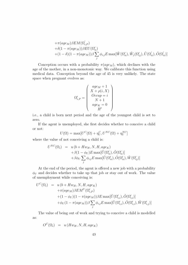
+π(ageM)βEM(Ω′i,P )

+δ(1− π(ageM))βEU(Ω′ii)

+(1− δ)(1− π(ageM))β∑

j

φi,jE max[W (Ω′ii), Wj(Ω

′ij), U(Ω

′ii), O(Ω

′ii)]

Conception occurs with a probability π(ageM), which declines with theage of the mother, in a non-monotonic way. We calibrate this function usingmedical data. Conception beyond the age of 45 is very unlikely. The statespace when pregnant evolves as:

Ω′i,P =

ageM + 1X + ρ(i,X)Occup = i

N + 1ageK = 0

H ′

i.e., a child is born next period and the age of the youngest child is set tozero.

If the agent is unemployed, she first decides whether to conceive a childor not:

U(Ω) = max[UC(Ω) + ηCU , UNC(Ω) + ηNC

U ]

where the value of not conceiving a child is:

UNC(Ωi) = u (b + HwH , N, H, ageK)

+β(1− φU)E max[U(Ω′ii), O(Ω′

ii)]

+βφU

∑

j

φi,jE max[U(Ω′ii), O(Ω′

ii), W (Ω′ij)]

At the end of the period, the agent is offered a new job with a probabilityφU and decides whether to take up that job or stay out of work. The valueof unemployment while conceiving is:

UC(Ωi) = u (b + HwH , N, H, ageK)

+π(ageM)βEMU(Ω′i,P )

+(1− φU)(1− π(ageM))βE max[U(Ω′i,i), O(Ω′

i,i)]

+φU(1− π(ageM))β∑

j

φi,jE max[U(Ω′i,i), O(Ω′

i,i), W (Ω′i,j)]

The value of being out of work and trying to conceive a child is modelledas:

OC(Ωi) = u (HwH , N, H, ageK)

49

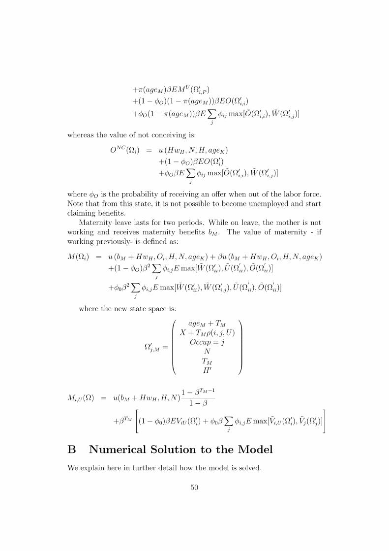
+π(ageM)βEMU(Ω′i,P )

+(1− φO)(1− π(ageM))βEO(Ω′i,i)

+φO(1− π(ageM))βE∑

j

φij max[O(Ω′i,i), W (Ω′

i,j)]

whereas the value of not conceiving is:

ONC(Ωi) = u (HwH , N,H, ageK)

+(1− φO)βEO(Ω′i)

+φOβE∑

j

φij max[O(Ω′i,i), W (Ω′

i,j)]

where φO is the probability of receiving an offer when out of the labor force.Note that from this state, it is not possible to become unemployed and startclaiming benefits.

Maternity leave lasts for two periods. While on leave, the mother is notworking and receives maternity benefits bM . The value of maternity - ifworking previously- is defined as:

M(Ωi) = u (bM + HwH , Oi, H, N, ageK) + βu (bM + HwH , Oi, H, N, ageK)

+(1− φO)β2∑

j

φi,jE max[W (Ω′ii), U(Ω

′ii), O(Ω

′ii)]

+φ0β2

∑

j

φi,jE max[W (Ω′ii), W (Ω′

i,j), U(Ω′ii), O(Ω

′ii)]

where the new state space is:

Ω′j,M =

ageM + TM

X + TMρ(i, j, U)Occup = j

NTM

H ′

Mi,U(Ω) = u(bM + HwH , H, N)1− βTM−1

1− β

+βTM

(1− φ0)βEViU(Ω′

i) + φ0β∑

j

φi,jE max[Vi,U(Ω′i), Vj(Ω

′j)]

B Numerical Solution to the Model

We explain here in further detail how the model is solved.

50

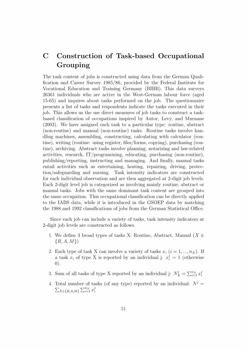
C Construction of Task-based Occupational

Grouping

The task content of jobs is constructed using data from the German Quali-fication and Career Survey 1985/86, provided by the Federal Institute forVocational Education and Training Germany (BIBB). This data surveys26361 individuals who are active in the West-German labour force (aged15-65) and inquires about tasks performed on the job. The questionnairepresents a list of tasks and respondents indicate the tasks executed in theirjob. This allows us the use direct measures of job tasks to construct a task-based classification of occupations inspired by Autor, Levy, and Murnane(2003). We have assigned each task to a particular type: routine, abstract(non-routine) and manual (non-routine) tasks. Routine tasks involve han-dling machines, assembling, constructing, calculating with calculator (rou-tine), writing (routine: using register, files/forms, copying), purchasing (rou-tine), archiving. Abstract tasks involve planning, notarizing and law-relatedactivities, research, IT/programming, educating, purchasing (non-routine),publishing/reporting, instructing and managing. And finally, manual tasksentail activities such as entertaining, hosting, repairing, driving, protec-tion/safeguarding and nursing. Task intensity indicators are constructedfor each individual observation and are then aggregated at 2-digit job levels.Each 2-digit level job is categorized as involving mainly routine, abstract ormanual tasks. Jobs with the same dominant task content are grouped intothe same occupation. This occupational classification can be directly appliedto the IABS data, while it is introduced in the GSOEP data by matchingthe 1988 and 1992 classifications of jobs from the German Statistical Office.

Since each job can include a variety of tasks, task intensity indicators at2-digit job levels are constructed as follows.

1. We define 3 broad types of tasks X: Routine, Abstract, Manual (X ∈R,A, M)

2. Each type of task X can involve a variety of tasks xi (i = 1, ..., nX). Ifa task xi of type X is reported by an individual j: xj

i = 1 (otherwise0).

3. Sum of all tasks of type X reported by an individual j: N jX =

∑nXi=1 xj

i

4. Total number of tasks (of any type) reported by an individual: N j =∑X∈R,A,M

∑nXi=1 xj

i

51

5. Intensity of type X tasks reported by individual j: ijX = N jX/N j.

6. Each observation (j=1,...,N) belongs to a 2-digit job category Y. Taskintensities are aggregated over all observations j in a 2-digit job categoryY (j ∈ Y , nY observations). Task intensity of type X in job categoryY: IY

X = 1nY

∑j∈Y ijX

52

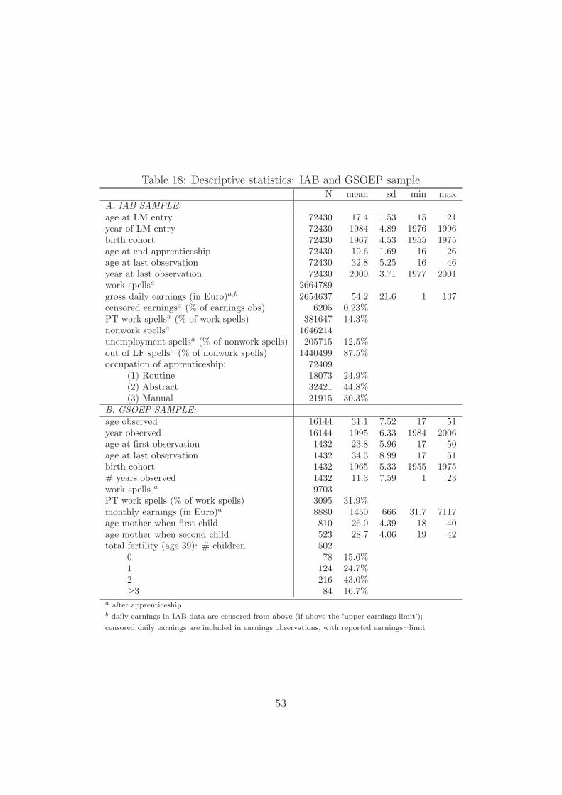
Table 18: Descriptive statistics: IAB and GSOEP sampleN mean sd min max

A. IAB SAMPLE:age at LM entry 72430 17.4 1.53 15 21year of LM entry 72430 1984 4.89 1976 1996birth cohort 72430 1967 4.53 1955 1975age at end apprenticeship 72430 19.6 1.69 16 26age at last observation 72430 32.8 5.25 16 46year at last observation 72430 2000 3.71 1977 2001work spellsa 2664789gross daily earnings (in Euro)a,b 2654637 54.2 21.6 1 137censored earningsa (% of earnings obs) 6205 0.23%PT work spellsa (% of work spells) 381647 14.3%nonwork spellsa 1646214unemployment spellsa (% of nonwork spells) 205715 12.5%out of LF spellsa (% of nonwork spells) 1440499 87.5%occupation of apprenticeship: 72409

(1) Routine 18073 24.9%(2) Abstract 32421 44.8%(3) Manual 21915 30.3%

B. GSOEP SAMPLE:age observed 16144 31.1 7.52 17 51year observed 16144 1995 6.33 1984 2006age at first observation 1432 23.8 5.96 17 50age at last observation 1432 34.3 8.99 17 51birth cohort 1432 1965 5.33 1955 1975# years observed 1432 11.3 7.59 1 23work spells a 9703PT work spells (% of work spells) 3095 31.9%monthly earnings (in Euro)a 8880 1450 666 31.7 7117age mother when first child 810 26.0 4.39 18 40age mother when second child 523 28.7 4.06 19 42total fertility (age 39): # children 502

0 78 15.6%1 124 24.7%2 216 43.0%≥3 84 16.7%

a after apprenticeshipb daily earnings in IAB data are censored from above (if above the ’upper earnings limit’);

censored daily earnings are included in earnings observations, with reported earnings=limit

53