The Capital Asset Pricing ModelThe Capital Asset Pricing Model

Lecture XXIV

.Literature.Literature

Most of today’s materials comes from Eugene F. Fama and Merton H. Miller The Theory of Finance (Hinsdale, Illinois: Dryden Press, 1972) Chapter 7.

The primary literature is: Lintner, John. “Security Prices, Risk, and

Maximal Gain from Diversification.” Journal of Finance 20(Dec. 1965): 587-615.

Lintner, John. “The Valuation of Risk Assets and the Selection of Risky Investments in Stock Portfolios and Capital Budgets.” Review of Economics and Statistics 47(Feb. 1965): 13-37.

Mossin, Jan. “Equilibrium in a Capital Asset Market.” Econometrica 34(Oct. 1966): 768-83.

Sharpe, W. F. “Capital Asset Prices: A Theory of Market Equilibrium under Conditions of Risk.” Journal of Finance 19(Sept. 1964): 425-42.

Setting Up the Market

Perfect Markets: We assume that all markets are competitive for goods and investments. All goods and investments are infinitely divisible. Information is costless. There are no transaction costs. No individual is large enough to effect the price.

Firms: All goods are produced by firms. These firms purchase the factors of production

in the first period, produce output, and market their goods in the second period.

In addition, these firms do not have any capital of their own and must raise this capital by issuing stock.

Consumers: Consumers begin with an endowment w1. The consumer’s choice problem (initially) is twofold. First, the consumer must decide how much to

consume in this period, c1, and how much to invest, h1. This investment will earn a rate of return h1(1+Ri) which will be consumed in the second period, c2.

Second, the consumer must decide how to invest h1, that is how to divide it up between a wide array of assets.

In general, this implies two decision dimensions. The first is intertemporal (across time). In this decision the consumer has a time preference, the preference between consuming now and consuming later.

c1

c2

1/(1+r)U(c1,c2)

The second is the risk or uncertainty on the investment. Both of these questions can be represented in the utility function.

Market Equilibrium: Assuming that firms supply investment and consumers demand investment opportunities, we hypothesize that there exists an equilibrium where the supply of stocks equals the demand of stocks.

..Risk Equilibrium From the Consumer’s Point of View

At the outset, we assume that consumers are risk averse and that risk can be characterized using the normal distribution function. Given these assumptions, we can use the

Expected Value-Variance, or in this case the Expected Value-Standard Deviation approach to expected utility/risk efficiency.

where p is the expected return from the portfolio, i is the expected return on a specific asset, and xi is the level of asset i held in a specific portfolio.

N

iiip x

1

~

Similarly, the standard deviation of the portfolio can be written as

where p is the standard deviation of a particular portfolio and ij is the covariance between asset i and asset j.

21

1 1

~~

N

j

N

ijiijp xx

In addition, we impose a portfolio balance condition

1~1

N

iix

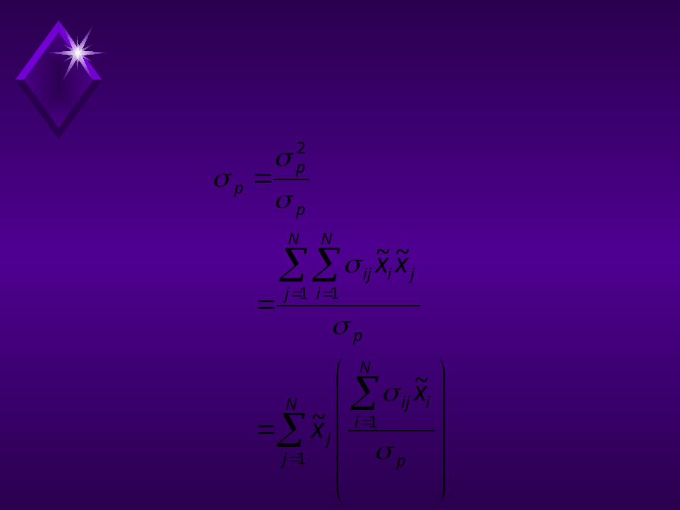
We can reformulate the risk measure, standard deviation of the portfolio, to analyze the contribution of each asset to the overall risk of the portfolio:

N

j p

N

iiij

j

p

N

j

N

ijiij

p

pp

xx

xx

1

1

1 1

2

~~

~~

The risk of a particular asset xj is then dependent on weighted covariances between asset j and the returns in the rest of the portfolio. Remember that the xis are weights in the general portfolio. This raises two points: First, note that the risk of an individual asset

depends on the portfolio weights and the risk of the portfolio.

Second, the risk of a particular asset depends both on its own variance and the variance of the remaining assets in the portfolio. Thus, as the number of assets becomes large and the portfolio becomes well diversified, the risk of a particular asset is more dependent on the covariance with other assets in the portfolio than on its own risk.

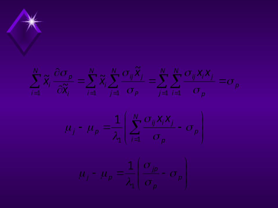
Following our previous discussions of Expected Value-Variance frontier, we assume that consumers choose the portfolio that minimizes risk for any given level of expected income. However, in this case risk is parameterized by the standard deviation instead of the variance.

1~

~..

~~min

1

*

1

21

1 1

N

ii

N

iiip

N

j

N

iijijp

x

xts

xx

0~1

0~

0~~

~1~

12

11

21

12

11

N

ii

N

iiip

kk

p

k

N

ii

N

iiipp

xL

xL

xx

L

xxL

k

p

l

plk

ll

pk

k

p

xx

xx

~~1

~~

1

11

p

p

N

i i

pi

N

i j

piij

N

ii x

xx

xx1111

~~

~~1~

N

i i

pi

j

ppj x

xx 11

~~

~1

N

j P

N

iiik

k

p

p

N

iiij

jp

x

x

xx

1

11

~

~

~~

p

N

j

N

i p

jiijN

i

N

j P

jiji

N

i i

pi

xxxx

xx

1 11 11

~~

~~

p

N

i p

jiijpj

xx

11

1

p

p

jppj

1

1

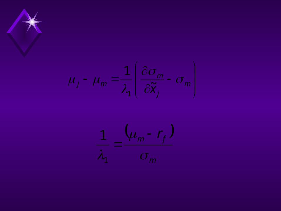
The Role of the Riskless Asset

The equilibrium presented above does not yield an estimable representation because different investors may have different risk preferences. One way around this ambiguity is to introduce a riskless asset. The riskless asset reduces the potential number

of efficient portfolios to a single portfolio.

p

p

rf

p

rp

Within this equilibrium, there is only one efficient portfolio of assets. Any degree of risk aversion can construct a risk preferred position by holding a combination of the single efficient portfolio and borrowing or lending at the riskless rate.

Substituting xm for xp or letting the index portfolio be the market efficient portfolio, we have

mj

mmj x

~1

1

m

fm r

1

1

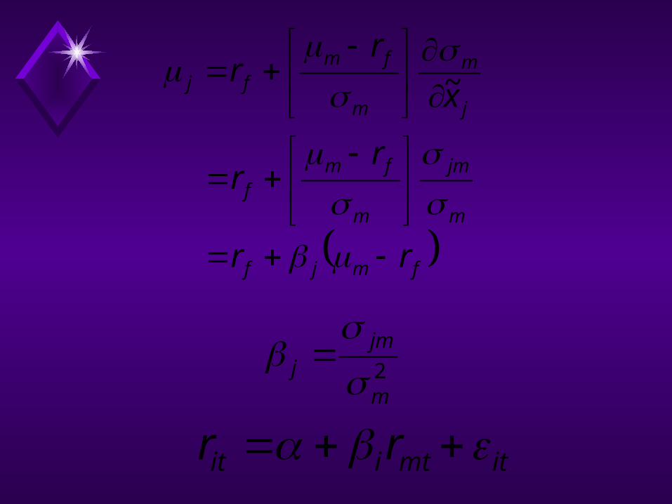
fmjf

m

jm

m

fmf

j

m

m

fmfj

rr

rr

x

rr

~

2m

jmj

itmtiit rr

Supply of Stocks from the Firm

We start by assuming that each firm sells stocks at a price Pi. Investors are willing to bid on these stocks based on the future value of the firm at the end of the year, Vi. The bid price and the value at the end of the year determine the rate of return:

i

iii P

PVR

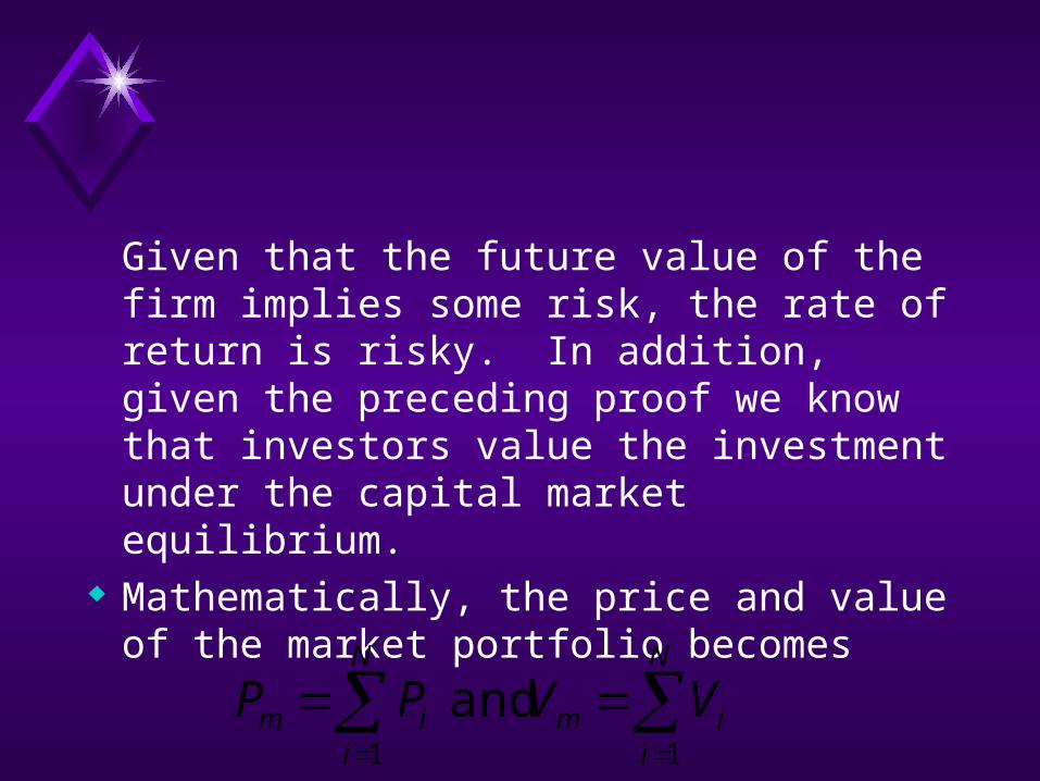
Given that the future value of the firm implies some risk, the rate of return is risky. In addition, given the preceding proof we know that investors value the investment under the capital market equilibrium.

Mathematically, the price and value of the market portfolio becomes

N

iim

N

iim VVPP

11

and

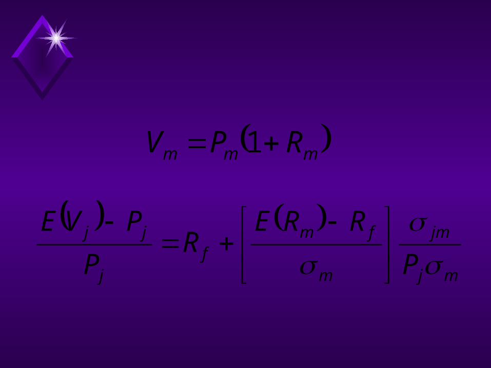
mmm RPV 1

mj

jm

m

fmf

j

jj

P

RRER

P

PVE

Incorporating Risk Using CAPM

Both risk adjustments come directly from the last equation. The first approach is referred to as the risk adjusted discount rate (RADR). Reducing the preceding expression to the CAPM formula

fmjfj RRRR

This risk adjusted discount rate can be used in present value analysis

N

ii

fmjf

t

RRR

ICFEPV

1 1

Reformulating this equality slightly

This approach leads to transforming the annual rates of return into “certainty equivalents” based on the market portfolio:

fMfjj

RRRR 1

N

ii

m

tj

R

ICFEPV

1 1

1