Embed Size (px)
Citation preview

THE BUSINESS SCHOOL FOR FINANCIAL MARKETS
The University of Reading
Common Trends, Mean Reversion and Herding:
Sources of Abnormal Returns in Equity Markets
ISMA Centre Discussion Papers in Finance 2003-08 First version: May 2003 This version: July 2003
Carol Alexander ISMA Centre, University of Reading, UK
Anca Dimitriu
ISMA Centre, University of Reading, UK
Copyright 2003 Carol Alexander and Anca Dimitriu. All rights reserved.
The University of Reading • ISMA Centre • Whiteknights • PO Box 242 • Reading RG6 6BA • UK Tel: +44 (0)118 931 8239 • Fax: +44 (0)118 931 4741 Email: [email protected] • Web: www.ismacentre.rdg.ac.uk Director: Professor Brian Scott-Quinn, ISMA Chair in Investment Banking The ISMA Centre is supported by the International Securities Market Association

Abstract In the field of optimisation models for passive investments, we propose a general portfolio construction
model based on principal component analysis. The portfolio is designed to replicate the first principal
component of a group of stocks, instead of an equally weighted or value weighted benchmark, thus
capturing only the common trend in the stock returns. The main advantage of this approach is that the
reduction of the noise present in stock returns facilitates the replication task considerably and the optimal
portfolio structure is very stable. We show that the strategy exploits the mean reversion in stock returns
and it over-performs a price-weighted benchmark of US stocks on a risk-adjusted basis, even after
transaction costs. We analyse the portfolio performance over different time horizons and in different
international equity markets and find a significant time-variability in the behaviour of the abnormal
returns. In addition to the market returns, other determinants of the abnormal returns are a value index
and the implied growth rate in stock returns. Behavioural explanations for the mean reversion mechanism
lead to the conclusion that the abnormal return is influenced by the extent of investors’ herding towards
the common trend in stock returns.
Author Contacts: Prof. Carol Alexander Chair of Risk Management and Director of Research ISMA Centre, School of Business, University of Reading, Reading RG6 6BA Email: [email protected] Anca Dimitriu (corresponding author) ISMA Centre, School of Business University of Reading, Reading RG6 6BA Tel +44 (0)118 9316494 Fax +44 (0)118 9314741 Email: [email protected] JEL classification: C32, C51, G11, G23
Keywords: common trends, mean reversion, herding, principal component analysis, abnormal returns, value strategies, behavioural finance
The authors would like to thank Glen Larsen for his valuable comments on the behavioural implications of our results. All errors remain our responsibility. This discussion paper is a preliminary version designed to generate ideas and constructive comment. The contents of the paper are presented to the reader in good faith, and neither the author, the ISMA Centre, nor the University, will be held responsible for any losses, financial or otherwise, resulting from actions taken on the basis of its content. Any persons reading the paper are deemed to have accepted this.
ISMA Centre Discussion Papers in Finance DP2003-08
Introduction
Comparisons between the two main equity investment styles – active and passive – have a long
history, being much influenced by both academic research and the investment management
industry.1 The interest in replicating market performance through a passive strategy, most
frequently in the form of indexation, is substantiated by the principles of efficient markets and
modern portfolio theory, where the only way that investors can beat the market over the long term
is by taking greater risks (Fama, 1970). Additionally, active management has been shown to
under-perform its passive alternative (Jensen, 1968; Elton, Gruber, Das, Hlavka, 1993;
Carhart, 1997) often due to transaction costs and administration fees, mostly in bull, but also in
bear markets. For example, the S&P active/passive scorecard for the last quarter of 2002 shows
that the majority of active funds have failed to beat their relevant index even in the bear market of
the last few years. As a consequence of these trends, the passive investment industry has
witnessed a remarkable growth during the last ten years, with a huge number of funds pegging
their holdings to broad market indexes such as SP500. Currently, it is estimated that more than
$1.4 trillion are invested in index funds in the US alone (Blake, 2002).
Traditionally, indexation has targeted price-weighted and capitalisation-weighted indexes, the
latter being easy to replicate with portfolios comprising the entire set of stocks and mirroring the
benchmark weights. Such portfolios are self-adjusting to changes in stock prices and do not
require any rebalancing, provided there are no changes in the index weights and composition or in
the number of shares in each issue. Despite the self-replication advantage, holding all the stocks
in the benchmark may not always be desirable or possible.2 More involved strategies are required
for tracking price-weighted indexes, since frequent rebalancing is required in order to maintain
equal dollar amounts in each stock. A thorough empirical investigation of the relationship
between the indexed portfolio’s composition and the tracking performance is provided by Larsen
and Resnick (1998). Their results show that value weighted indexes are easier to replicate than
equally weighted indexes, and capitalisation dominates other stratification criteria such as
industry classification.
1 As a consequence, the very concepts of active and passive investment styles have evolved. Now, they can only be discriminated based on their investment objective, all other features, e.g. amount of research involved, portfolio optimisation techniques, frequency of trades, being similar. The active management is seeking to over-perform the market, usually through stock selection or market timing, while passive management is aiming to replicate the market performance. Also, strategies such as enhanced index tracking, which extend a passive style into active management, have been developed. 2 This happens mainly because of difficulties in purchasing odd lots to exactly match the market weights, or the increased transaction costs/market impact related to trading less liquid stocks.
Copyright © 2003 Carol Alexander and Anca Dimitriu 3

ISMA Centre Discussion Papers in Finance DP2003-08
Given these disadvantages of direct replication, recent research has focussed on developing
optimisation models for passive investments. Conventionally, tracking strategies using fewer
stocks are constructed on basic capitalisation or stratification considerations. Optimisation
techniques have also been developed using objective functions based on: the correlation of the
portfolio returns with the benchmark; the mean deviation of the tracking portfolio returns from
the benchmark; the variance of this deviation (often referred to as ‘tracking error’); or on
transaction costs. Some examples are given in Rudd (1980), Meade and Salkin (1989), Adcock
and Meade (1994), Connor and Leland (1995), Alexander (1999), Larsen and Resnick (1998 and
2001). The present paper contributes to this line of research by proposing a general portfolio
construction model based on principal component analysis. The model identifies, of all possible
combinations of stocks with unit norm weights, the portfolio that captures the largest amount of
the total joint variation of the stock returns. Such a property makes it the optimal portfolio for
capturing the common trend in a system of stocks whilst filtering out a significant amount of
noise.
In finance, the use of statistical techniques to model asset returns has been extensive, especially in
the context of factor models. Going back to Feeney and Hester (1967) and Lessard (1973), or in
more recent years, Schneeweiss and Mathes (1995) and Chan, Karceski and Lakonishok (1998),
principal component and factor analysis have been used to examine the existence of common
movements in stock returns. They are seen as alternatives to fundamental approaches which
relate the factors influencing financial asset returns to macroeconomic measures such as inflation,
interest rates, and market indices, or to company specifics such as size, book to market ratio or
dividend yield.
A great deal of statistical factor-type of analysis has been performed for testing the arbitrage
pricing model (Ross, 1976). In this context, historical returns are used to estimate orthogonal
statistical factors and their relationship with the original variables. The construction of
mimicking portfolios for the statistical factors has been formalised by Huberman, Kandel and
Stambaugh (1987). Furthermore, alternatives to standard principal component analysis have been
developed, e.g. asymptotic PCA (Chamberlain and Rotschild, 1983, Connor and Korajczyk, 1986
and 1988) or independent component analysis (Common, 1994).
Copyright © 2003 Carol Alexander and Anca Dimitriu 4

ISMA Centre Discussion Papers in Finance DP2003-08
One aspect that is often scrutinised is the number of factors that are relevant for explaining stock
returns. Chan, Karceski and Lakonishok (1998) demonstrate that, in a predictive sense, there is
no benefit from using more than two or three principal components to explain stock returns.
More importantly, their results suggest that the first principal component is, in essence, capturing
the market factor. Similar findings have been previously reported by Connor and
Korajczyk (1988). In their paper, the R2 from a simple regression of the monthly returns of an
equally-weighted portfolio on the first principal component of the stock returns is 0.99. Based on
this result, the first principal component is seen as representing the stock market. Our portfolio
construction model is based precisely on the resemblance of the first principal component of the
stock returns to the market factor proxied by a traditional index.
The standard approach to constructing factor mimicking portfolios uses the factor loadings in the
stock selection process (Fama and French, 1993). The stocks are ranked according to their
loading on a particular factor, then a self-financed portfolio is set up with long positions on the
stocks with the highest loadings on that factor and short positions on the stocks with the smallest
loadings. Most frequently, there is no portfolio optimisation, equal dollar amounts being invested
in each stock. An alternative proposed by Fung and Hsieh (1997) for factor mimicking portfolios
considers, in the stock selection stage, only the stocks that are highly correlated solely to the
principal component for which the replica is constructed. Having selected the stocks, their
portfolio weights are optimised as to deliver the maximal correlation of the mimicking portfolio
returns with the corresponding principal component.
In these two methods, principal component analysis is used as a stock selection technique and the
portfolio construction is a separate stage, based either on a standard optimisation, or on an
arbitrary method such as equal weighting. In this paper we propose a different approach in which
a portfolio replicating the first principal component is constructed directly from the normalised
eigenvectors of the covariance matrix of stock returns. Such a portfolio, by construction, captures
the largest proportion of the variation in the stock returns and filters out a significant amount of
noise. Therefore, it is naturally suited for a passive investment framework: it requires a fully
invested portfolio of all stocks, but this involves a very small amount of rebalancing trades
because it captures only the major common trend in stock returns. This procedure involves a
single optimisation, the one producing the principal components. Moreover, there is no arbitrary
choice of the portfolio construction model, such as equal weighting of stocks.
Copyright © 2003 Carol Alexander and Anca Dimitriu 5
ISMA Centre Discussion Papers in Finance DP2003-08
In order to investigate the model performance, we have used stocks included in the Dow Jones
Industrial Average (DJIA) at the end of year 2002. To support the features of the strategy
observed in the DJIA case, we have also constructed random subsets of stocks from SP100,
FTSE100 and CAC40. The model performance is analysed both before and after transaction
costs: we examine the returns volatility and correlation (unconditional over the entire sample and
also short-term time series estimates), and the higher order moments of returns distributions, both
from an overall perspective and conditional on market circumstances.
Unsurprisingly, our results indicate that the first principal component captures the market factor,
being highly correlated with the benchmark returns and having similar information ratios.
Moreover, the factor weights prove to be very stable in time, so transactions costs are minimal.
However, what does come as some surprise is that, out of sample, the portfolio replicating the
first principal component, while being highly correlated with a price-weighted benchmark, is
significantly over-performing it. Subsequently we demonstrate that the cause of the over-
performance is a mean reversion in returns, for the group of stocks which are over-weighted by
the portfolio. These are the stocks that have had higher volatility and have also been highly
correlated as a group, during the portfolio calibration period. We observe two behavioural
mechanisms which could explain the mean reversion for these stocks: the attention capturing
effect documented by Odean (1999) and the over-reaction based models of De Long, Shleifer,
Summers and Waldmann (19901), Lakonishok, Shleifer and Vishny (1994) and Shleifer and
Vishny (1997). Separately, our results show that the abnormal return3 is related to a behavioural
measure of the investors’ herding towards the market factor, driving the mean reversion in stock
returns.
The analysis of the abnormal returns obtained in DJIA universe reveals two patterns in the
relationship with the benchmark: in the first pattern, prevailing through the largest part of the data
sample and during which mean reversion is effective, the factor mimicking portfolio has a small
beta, but a significant alpha term associated with negative returns; in the second pattern,
occurring during the last few years when the normal mean reversion cycle is broken, the portfolio
has a beta higher than one, and it is now this that explains the abnormal return.
3 We define the abnormal return as the difference between the factor mimicking portfolio returns and a price weighted benchmark reconstructed from the same stocks as the portfolio.
Copyright © 2003 Carol Alexander and Anca Dimitriu 6
ISMA Centre Discussion Papers in Finance DP2003-08
Subsequently, a factor model is estimated for the abnormal return obtained in the DJIA universe.
The estimated model indicates as significant explanatory variables, in addition to the benchmark
returns and some slope dummy variables which account for the two patterns identified above, the
SP500 BARRA value index and the implied economic growth rate in stock prices. The factor-
mimicking portfolio is found to have a significant value component, which justifies part of the
over-performance throughout the sample, and we show that this is consistent with our behavioural
explanation for the abnormal returns. Note that the value-like performance is obtained with a
portfolio of blue chips, having much more attractive features than a standard value strategy.
The remainder of the paper is organised as follows: section one introduces the model for the first
principal component portfolio, section two describes the data and the performance testing
methodology, section three reviews the in-sample statistical properties of the first principal
component, section four analyses the out-of-sample performance of the first principal component
portfolio, section five reports the results of the strategy on other market indexes, and finally,
section six summarises and concludes.
I. The first principal component portfolio model
Principal component analysis (PCA), introduced by Hotelling (1933) in connection to the analysis
of data in psychology, was recommended as an important tool in the multivariate analysis of
economic data more than half a century ago (Tintner, 1946). This technique is now a standard
procedure for an orthogonal transform of variables, reducing dimensionality and the amount of
noise in the data.
Given a set of k stationary random variables, X1, X2, ...Xk, PCA determines linear combinations of
the original variables, called principal components and denoted by P1, P2,... Pk, so that (1) they
explain, successively, the maximum amount of variance possible and (2) they are orthogonal. By
convention, the first principal component is the linear combination of X1, X2, ...Xk that explains
the most variation. Each subsequent principal component accounts for as much as possible from
the remaining variation and is uncorrelated with the previous principal components.
The ith principal component, where i = 1, ..., k, may be written:
Pi = w1iX1 + w2iX2 + ...+ wkiXk (1)
Copyright © 2003 Carol Alexander and Anca Dimitriu 7

ISMA Centre Discussion Papers in Finance DP2003-08
Thus, if we denote by Σ the covariance matrix of X, then:
var(Pi) = wi′ Σ wi ;
cov(Pi, Pj) = wi′ Σ wj,
where wi = [w1i w2i ...wki]′ and it is standard to impose the restriction of unit length for these
vectors, i.e. wi′wi = 1.4 Note that these are, in fact, the eigenvectors of Σ: the spectral
decomposition of the covariance matrix is Σ = WΛW′, where Λ is a diagonal matrix of
eigenvalues (ordered by convention so that 0...21 >>>> kλλλ ) and W is an orthogonal matrix
of eigenvectors (which have also been ordered according to the size of the corresponding
eigenvalue); now principal components defined as P = XW observe the conditions above.
Note that the variance of each principal component is equal to the corresponding eigenvalue, so
the total variability of the system is the sum of all eigenvalues. To reproduce the total variation
of a system of k variables, one needs exactly k principal components. However, when the first
few principal components together account for a large part of the total variability, the
dimensionality – and much of the noise in the original data – can be significantly reduced.
Since the principal components define a k-dimensional space in terms of orthogonal coordinates,
the distances defined in the principal components space depend on the amount of correlation in
the original variables. The higher the correlation in the original system, the better a principal
component can account for the original joint variation and the larger the inter-point distances will
be in that dimension. The elements of the first eigenvector are the factor loadings on the first
principal component in the representation of the variables in terms of principal components. In a
highly correlated system, these elements will be of similar size and sign. Consequently, if
portfolio weights were directly proportional to the elements of the first eigenvector, as in (2)
below, the more highly correlated the stocks, the more evenly balanced the portfolio.
When applied to large stock universes, previous research has shown that the first principal
component is capturing the market factor, explaining a very high proportion from the returns of
an equally-weighted portfolio of all stocks. Motivated by these results, we propose a portfolio
4 Eigenvectors are not unique, and so it is standard to impose the orthonormal constraint. A more natural constraint in a portfolio construction framework would be to have the sum of the eigenvectors, rather than the sum of their squares, equal to one. However, this does not ensure a balanced portfolio structure, which is essential for indexing. In order to avoid large exposures to individual stocks, we keep the unit length constraint for the eigenvectors, and then normalise them to sum up to one.
Copyright © 2003 Carol Alexander and Anca Dimitriu 8
ISMA Centre Discussion Papers in Finance DP2003-08
construction model which is based on replicating the first principal component of a set of stock
returns.5
For a portfolio of k stocks, the portfolio weight of stock i is defined as:
∑=
=k
jjii www
111 / (2)
where wi1 is the ith element from the first column in the eigenvectors matrix ordered as above.
In the PCA framework described above, the first eigenvector is obtained, independently of the
others, by maximising the variance of the corresponding linear combination of stocks, under the
constraint of unit norm. Therefore the portfolio based on the stock weights determined as in (2)
is, of all possible combinations of k stocks with unit norm, the portfolio that accounts for the
largest part of the total joint variation of the k stocks. This property ensures that it is the optimal
portfolio for capturing the common trend in a system of stocks. Considering that the model
maximises the variance of the portfolio under some constraint, it will over-weight, relative to
benchmark, the stocks that were both highly correlated and had higher than average volatility
over the estimation period.
II. Data and portfolio ‘out-of-sample’ returns
In order to examine the properties of the portfolio replicating the first principal component, we
use a main data set comprising daily close prices on the 25 stocks currently included in the DJIA
and which have a history available for the period Jan-80 to Dec-02. Four out of the five stocks
which are currently in the DJIA, but which do not have a history going back to Jan-80, are
technology stocks. Therefore, our portfolio has a lower loading on technology than the current
DJIA and the latter cannot be considered the relevant benchmark because of a ‘technology’ bias.
Also, the stock selection methodology may raise the concern of performance biases such as
survivorship and look-ahead, because we are selecting the stocks which had a history of at
least 23 years of data available. We deal with all these potential biases by creating a price-
5 We note that, often, the original stationary variables are standardised to have zero mean and unit variance before the principal component analysis – that is, that the eigenvectors of the correlation matrix are used to construct the principal components, rather than the eigenvectors of the covariance matrix. This ensures that the variable with the highest volatility does not dominate the first principal component. However, in a realistic portfolio construction setting, the assumption of equal volatilities for all assets is not feasible. Such an assumption would result in the portfolio model being constructed solely on the correlation structure of the assets, rather than the complete covariance structure of the data. Therefore, for the purpose of our model, we do not standardise the stock returns.
Copyright © 2003 Carol Alexander and Anca Dimitriu 9
ISMA Centre Discussion Papers in Finance DP2003-08
weighted benchmark from exactly the same stocks as our portfolio and analysing all performance
on a relative basis.
In addition to DJIA stocks, we use several sets of daily close prices of stocks included at the end
of year 2002 in the CAC40, FTSE100 and SP100 indexes. The length of the data sample ranges
from 1,600 daily observations for SP100 (Apr-96 to Jun-02) to 2,100 daily observations for
FTSE100 (Jul-94 to Dec-02). For each data set, we construct a price-weighted benchmark of all
the stocks in that particular set to be used in measuring the performance of our strategy.
For the purpose of performing principal component analysis, we are particularly interested in the
average correlation of the stock returns, as this has a strong influence on the effectiveness of the
first principal component to explain the variation of the stock returns. We find that the average
correlation of the daily stock returns from the DJIA set is in the range of 0.3 to 0.4, occasionally
going to as low as 0.2. The highest average correlation in stock returns occurs in down, volatile
markets, such as 1987, 1990, or 2001-2002, this being a common finding for stock markets.
Regarding the general market conditions during the sample period, it is worth mentioning that, in
10 out of the 23 years, the stocks in DJIA had average returns above 20%. By contrast, in only 5
years out of 23, the average return was negative, which, however, was the case for the last 3 years
in the sample. The average volatility stayed in the range of 20%-30%, increasing significantly in
the last part of the data sample. The year 1987 stands out from the sample, in terms of returns
correlation, volatility, excess kurtosis and negative skewness, because of the October crash.
The portfolio optimisation and rebalancing procedure is as follows: at each rebalancing moment,
the stock weights are determined from the eigenvectors of the covariance matrix of the stock
returns estimated from the most recent 250 observations prior to the moment of the portfolio
construction.6 For the out-of-sample performance assessment, the portfolio constructed in the
previous step is left unmanaged for the next 10-trading days, and then rebalanced based on the
new stock weights from principal component analysis. In order to account for transaction costs,
6 The ‘rolling sample’ PCA raises the issue of consistent identification of the factor loadings because the choice of the sign of the eigenvectors is arbitrary. Choosing a particular normalisation is not relevant if the estimation of the principal components is performed over the entire data sample. However, when the optimisation is performed over a rolling sample, in order to have consistent principal component estimates from successive estimations, one needs to ensure that the same normalisation is used throughout the entire data sample.
Copyright © 2003 Carol Alexander and Anca Dimitriu 10

ISMA Centre Discussion Papers in Finance DP2003-08
we assume an amount of 20 basis points on each trade value to cover the bid-ask spread and the
brokerage commissions, which is conservative for very liquid stocks such as those in the DJIA.
III. Empirical properties of the first principal component – in-sample analysis
Of central interest to our analysis are the eigenvectors of the covariance matrix of stock returns,
as these will determine the stock weights in the portfolio replicating the first principal component.
The eigenvector corresponding to the first principal component comprises the sensitivity of each
stock to changes in the first principal component, the so-called ‘factor loading’. As shown in (2),
the stock weights in the replicating portfolio are given by the factor loadings, normalised to sum
up to one. When the orthonormal convention for eigenvectors is employed (see footnote 4 in
section I), an implied leverage occurs in the first principal component portfolio, because the sum
of the elements of the first eigenvector will be far greater than one. Consequently, the absolute
returns on the first principal component computed with the orthonormal convention will be much
higher than those of the benchmark – as will the volatility of returns. The normalization
convention chosen has no effect on the information ratio (annual return divided by annual
volatility). Since re-scaling the eigenvectors has a similar impact on both absolute returns and
volatility, our choice of eigenvector convention is not relevant on a risk-adjusted basis. However,
for the specific purpose of portfolio construction, the orthonormal eigenvectors should be further
normalised to sum to unity. Only in this way will the portfolio weights (2) correspond a fully
invested portfolio.
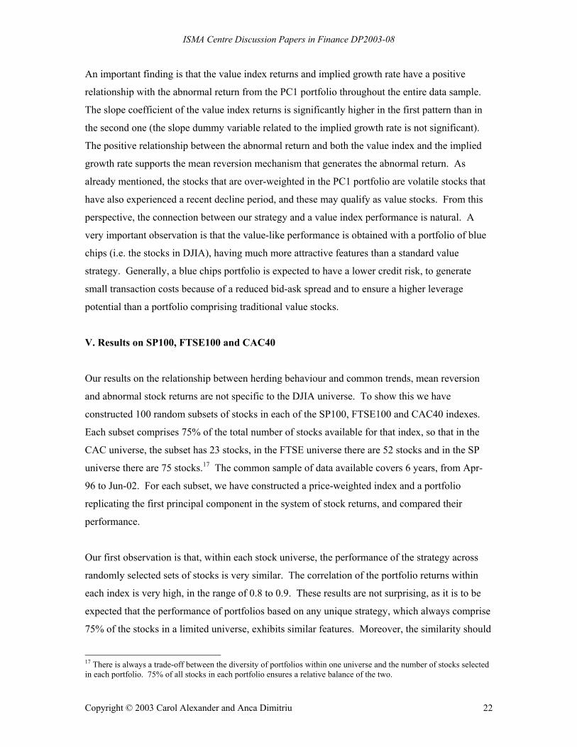
The information ratios for the benchmark and the first principal component, shown in Figure 1,
are very similar most of the time. Each point in Figure 1 represents the information ratio
computed in-sample, over the last 250 observations. The main exceptions are the periods 1985-
1986 and 1995-1996, during which the information ratios of the portfolio replicating the first
principal component are significantly higher. In addition to having similar information ratios, the
first principal component and the benchmark are also highly correlated. The correlation
coefficient ranges from 0.7 to 0.98. Lower correlation occurs between 1992 and 1996, but most
of the time it is still above 0.9. A standard regression of the benchmark returns on the first
principal component, estimated over the entire sample, has an R2 of 0.8. In summary, we can
safely conclude that the first principal component largely captures the market factor.
Copyright © 2003 Carol Alexander and Anca Dimitriu 11

ISMA Centre Discussion Papers in Finance DP2003-08
Given the connection between the first principal component and the market factor, the first
eigenvector can be thought of as a vector of market betas in a CAPM framework. If the stock
returns were perfectly correlated, the first principal component would capture the entire variation
of the system and the betas would all be equal to one. More generally, in a highly but not
perfectly correlated system, the factor weights on the first principal component will be similar but
not identical. This implies that, in highly correlated systems, a change in the first principal
component generates a nearly parallel shift in the original variables. For this reason, we identify
the first principal component with a ‘common trend’, if it exists.
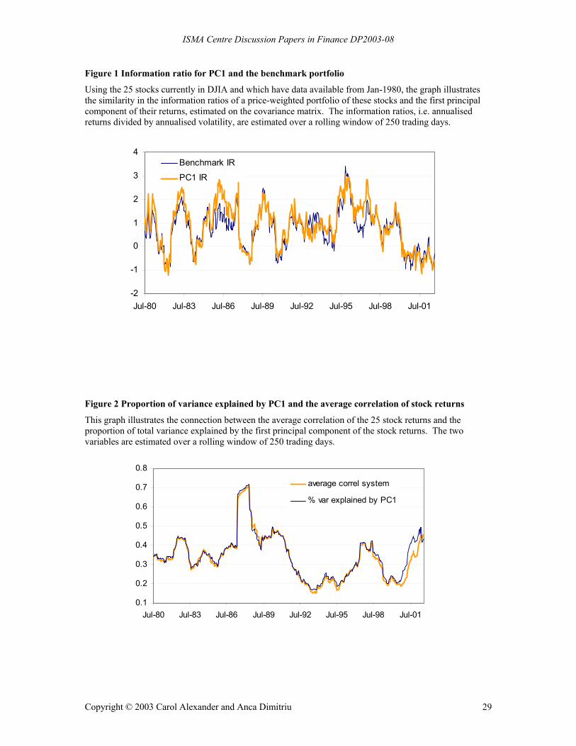
Regarding the amount of total variation explained by the first principal component, this turns out
to be in the range of 30-40%, in line with previous research on this issue. This is directly related
to the amount of correlation in the original system of returns. Figure 2 reports the proportion of
variance explained by the first principal component, along to the average correlation of returns.
The average correlation in the original data is the single most important determinant of the
proportion of variance explained by the first principal component.7 The lowest average
correlation (and, consequently, amount of variation explained by the first principal component)
occurs between 1992 and 1997, and again in 1999 and 2000. These times were relatively calm
periods for the developed stock markets, correlations being generally higher during more volatile
periods.
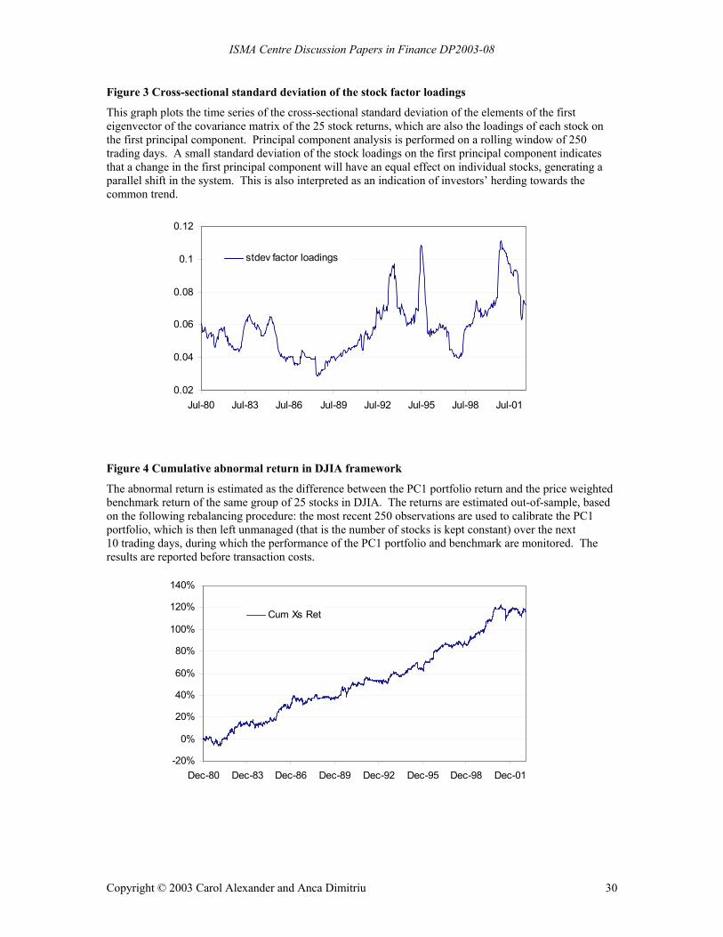
In the DJIA case, the factor loadings on the first principal component, i.e. the elements of the first
eigenvector, are largely in the same range: during periods of high average correlation (e.g. after
the 1987 crash) the factor loadings are high and very similar but more recently they tend to be
lower and less similar. This observation is justified by Figure 3, which plots the standard
deviation of the factor loadings. The similarity of the factor loadings is an important feature of
the model, as it allows the construction of balanced portfolios, without extreme exposures to
individual stocks. In fact, we observe that even though there are no short-sale restrictions
imposed on the model, short positions occur very rarely. Moreover, the dispersion of the factor
loadings has been used as a measure of herding behaviour in recent research in behavioural
finance (Hwang and Salmon, 2001), and we shall return to the implications of this issue in the
next section, analysing the out-of-sample performance of the model. Apart from the cross-
7 A ‘ghost feature’ caused by the October-87 crash can be identified in both of them: the correlation and the percentage of variance explained remain very high for as long as the October crash stays in the estimation sample and drop immediately after excluding that observation from the sample. This is an artefact of the euqal weighting in returns and would not be evident if exponential weighting of the covariance matrix were applied.
Copyright © 2003 Carol Alexander and Anca Dimitriu 12
ISMA Centre Discussion Papers in Finance DP2003-08
sectional variability of the factor loadings, a very attractive feature is their low time variability.
The factor loadings are very stable in time, which, in a portfolio construction setting, is translated
into a reduced amount of re-balancing trades and low transaction costs.
IV. Performance of the statistical factor equity portfolio – out-of-sample analysis
The portfolio is constructed from the 25 stocks that were both included in DJIA at the end of
2002 and had a history that goes back as far as Jan-80.8 The benchmark for the performance
assessment is a price-weighted portfolio with all 25 stocks. The portfolio replicating the first
principal component (denoted as PC1 portfolio) is first set up in Jan-81, based on the principal
component analysis performed on the 250 observations preceding the portfolio construction
moment and further rebalanced every 10-trading days. In between rebalancing, the number of
stocks in the portfolio is kept constant.
The performance statistics for the PC1 portfolio and the benchmark are reported in Table I. In
terms of annual returns, the PC1 portfolio over-performs the market by an average of 5% per
year, with only 1% extra volatility. The superior performance is also obvious in the information
ratios, 0.75 for the PC1 portfolio, as compared to 0.5 for the benchmark. Moreover, the
PC1 portfolio returns appear to be closer to normality than the returns on the benchmark
portfolio. The correlation between the two portfolio returns is very high, above 0.9. In terms of
transaction costs for implementing the strategy, they turn out to be almost negligible, amounting
to an average of 0.24% per year for the PC1 portfolio.9
If we interpret the abnormal return as the return on a self-financed strategy which, at each
moment in time, is long on the PC1 portfolio and short on the benchmark, then the 5.19% annual
return is associated with an annual volatility of 6.3%. Its information ratio is 0.82, higher than
those of the benchmark and PC1 portfolio. Moreover, the abnormal return is uncorrelated with
the benchmark return and much closer to normality than the latter.
8 We have also analysed the performance of a portfolio comprising all 30 stocks currently included in DJIA, over the period Jan-91 to Dec-02. The results are very similar to the ones obtained with the 25-stocks portfolio. For reasons of space, we have not included them in this paper. They are available by request from the authors. 9 As our target is to explain the ‘pure’ abnormal return, i.e. the difference between the PC1 portfolio return and benchmark return, after establishing that the overall profitability of the strategy does not disappear after transaction costs, we will perform the analysis of the abnormal return before transaction costs.
Copyright © 2003 Carol Alexander and Anca Dimitriu 13
ISMA Centre Discussion Papers in Finance DP2003-08
The returns from the PC1 portfolio and the benchmark portfolio turn out to have very similar
features also when analysed period by period. They are both affected by the main market crises
during the period in observation: Oct-87, the Gulf War, the Asian Crisis, the burst of the
technology bubble and Sep-01. The over-performance of the PC1 portfolio, as well as the fact
that it is not caused by singular events, are evident from Figure 4, which plots the cumulative
abnormal return. The abnormal return appears to be uniformly distributed in time, with few
exceptions – during the periods 1987-1990 and 2001-2002 it stays close to zero. On an annual
basis, the abnormal return on the PC1 portfolio is negative in only three out of 22 years: 1981,
1984 and 2001. The highest abnormal return, amounting to 20%, occurs in 2000. Moreover,
since the volatilities never rise above 10%, the abnormal return has an information ratio above
unity in 10 out of 22 years.
In terms of short-term volatility and correlation, the PC1 portfolio and the benchmark again have
very similar properties. The exponentially weighted moving average volatilities and correlation
for a smoothing parameter of 0.96 are shown in Figure 5. The volatility of the PC1 portfolio is
slightly higher, especially during the last part of the sample, but is closely following the
benchmark volatility. With very few exceptions, the correlation is high, staying above 0.8 most
of the time. As indicated by the behaviour of short-term volatilities, the correlation between the
PC1 portfolio and the benchmark is high also during market crises such as Oct-87 or Sep-01.
To summarise, the PC1 portfolio, while being highly correlated with the benchmark, produces a
significant abnormal return, which has a very low volatility and it is not correlated with the
benchmark on a daily frequency. Its third and fourth moments are much closer to normality than
those of the benchmark or PC1 portfolio.
A. A behavioural explanation of the abnormal return
As shown in section I, the stock weights are chosen to maximise the portfolio variance, subject to
the constraint of unit norm. Since portfolio variance increases with both individual asset variance
and the covariance between assets, the portfolio will over-weight, relative to the benchmark,
stocks that have higher volatility over the estimation period and which are also highly correlated
as a group. Separately, the benchmark, by being price-weighted, is under-weighting stocks that
have recently declined.
Copyright © 2003 Carol Alexander and Anca Dimitriu 14
ISMA Centre Discussion Papers in Finance DP2003-08
Now, if it does hold true that markets tend to be more turbulent after a large price fall than after a
similar price increase (i.e. the ‘leverage effect’ that is commonly identified in stock markets, as in
Black, 1976; Christie, 1982; French, Schwert and Stambaugh, 1987), then the same group of
stocks will be impacted through the over-weighting of volatile, correlated stocks in the PC1
portfolio and the under-weighting of declining stocks in the benchmark portfolio. These stocks
have had a volatile, declining period over the estimation sample. From this perspective, the over-
performance of the PC1 portfolio must be due to a mean reversion in stock returns over the one-
year estimation period used for our portfolio. The portfolio over-weights stocks that have
recently declined in price, relative to the benchmark, so the relative profit on the portfolio has to
be the result of a consequent rise in price of these stocks. The hypothesis that mean reversion
takes place over a period of one-year is supported by the fact that when the PC1 estimation
sample is reduced, the over-performance disappears.
Our result is also in line with the research on short-term momentum and long-term reversals that
has frequently been identified in stock returns. For example, De Bondt and Thaler (1985), Lo and
MacKinlay (1988), Poterba and Summers (1988) and Jagadeesh and Titman (1993) identify
positive autocorrelation in stock returns at intervals of less than one year and negative
autocorrelation at longer intervals. In behavioural finance, two explanations are usually proffered
for long-term reversals and short-term momentum in stock markets. The first explanation focuses
on relatively volatile stocks, which capture the attention of ‘noise traders’ for whom they are the
best buy candidates (Odean, 1999).10 The trading behaviour of noise traders creates an upward
price pressure on these volatile stocks, forcing mean reversion when their high volatility was
associated with a recent decline in price. The same explanation is not applicable to a selling
decision, creating symmetrically downward price pressure on volatile stocks, because the range of
choice in a selling decision is usually limited to the stocks already held (Barber and Odean,
2002). Additionally, we note that volatile stocks which have recently experienced a price decline,
also qualify as value stocks, and in section C we shall use this observation to explain the
connection between our strategy results and the performance of a value index.
10 Noise traders are usually defined in the literature as not fully rational investors, making investment decisions based on beliefs or sentiments which are not fully justified by fundamental news, or which are subject to a systematic biases.
Copyright © 2003 Carol Alexander and Anca Dimitriu 15

ISMA Centre Discussion Papers in Finance DP2003-08
A second behavioural explanation of the short-term momentum followed by mean reversion has
been provided by De Long, Shleifer, Summers and Waldmann (1990a), Lakonishok, Shleifer and
Vishny (1994) and Shleifer and Vishny (1997). This explanation is based on investors’
sentiment, over-reactions and excessive optimism/pessimism. The occurrence of some bad news
regarding one stock creates an initial excess volatility and, according to these models, some
investors will become pessimistic about that stock and start selling. If there is positive feedback
in the market, more selling will follow and the selling pressure will drive the price below its
fundamental level. However, the arbitrageurs (sometimes called ‘smart money’, or ‘rational’
investors) will not take positions against the mispricing either because (1) the mispricing is too
small to justify arbitrage after transaction costs, or (2) there is no appropriate replica available for
that stock, so the fundamental risk cannot be hedged away, or (3) there is a ‘noise trader risk’
arising from positive feed-back, where the excessive investors’ pessimism will drive the price
even further down in a short term. In the presence of positive feedback, De Long, Shleifer,
Summers and Waldmann (1990b) show that the arbitrageurs will initially join the noise traders in
selling, in order to close their positions when the mispricing has become even larger. This type of
investor behaviour justifies both short-term momentum and longer-term mean reversion.
In addition to the above explanations of the mean reversion in stock returns, which justify the
over-performance of the PC1 portfolio, we also find that there is a connection between the
abnormal returns generated by the PC1 portfolio and another behavioural phenomenon
documented in stock markets – investors’ herding. In this case, we will show that the more
intense the herding behaviour, as measured by a decrease in the cross sectional standard deviation
of the factor loadings, the higher the abnormal returns generated by the PC1 portfolio.
The use of the cross sectional distribution of stock returns as an indication of herding was first
introduced by Christie and Huang (1995) in the form of the cross sectional standard deviation of
individual stock returns during large price changes. Hwang and Salmon (2001) build on this idea
but instead advocate the use of a standardised standard deviation of factor loadings to measure the
degree of herding. Their measure has the advantage of capturing ‘intentional’ herding towards a
given factor, such as the market factor, rather than ‘spurious’ herding during market crises. They
find that herding towards the market happens especially during quiet periods for the market,
rather than when the market is under stress.
Copyright © 2003 Carol Alexander and Anca Dimitriu 16

ISMA Centre Discussion Papers in Finance DP2003-08
Following Hwang and Salmon (2001), we assume that the standard deviation of the factor
loadings (equivalently, the elements of the first eigenvector of the covariance matrix) captures the
intentional herding of the investors towards the first principal component of the stocks, or their
common trend. An intense herding of the investors towards the common trend of the stocks
should reduce the differences in the individual stocks loadings on the first principal component.
Therefore, we interpret a low standard deviation of the factor loadings as an indication of herding.
As shown by Figure 3, more intense herding appears to happen before 1993, and then again
before 1998, which supports the findings in Hwang and Salmon (2001) that herding occurs
especially during quiet periods for the market. During the market crises of the last five years, the
herding behaviour appears to be significantly reduced.
Considering the scenarios of mean reversion presented above, an intense herding towards the first
principal component, indicated by a sharp reduction in the standard deviation of the factor
loadings, is expected to enhance and speed up the mean reversion. Therefore the standard
deviation of the factor loadings should be negatively related to the abnormal returns generated by
the PC1 portfolio. Indeed, the correlation between the standard deviation of the factor loadings
and the abnormal return, estimated over all non-overlapping sub-samples of 250 observations, is
negative (-0.33) and significant at 5%. We conclude that the more intense the herding towards
the first principal component, the higher the abnormal returns generated by the PC1 portfolio.
To summarise, the PC1 portfolio has been shown to produce consistent return in excess of the
benchmark by exploiting one of the most commonly documented phenomenon in the stock
markets, i.e. the long-term mean reversion in the stock returns, which is usually explained by
behavioural considerations. Indeed, the abnormal return has been shown to be proportional to a
measure of investors’ herding towards the common trend in stock returns.
B. Analysis of the abnormal return in different market conditions
Apart from the general considerations about the mechanism producing the abnormal return, we
are also interested in analysing the performance of the strategy in different market circumstances
and over different time periods, as it is very unlikely that the strategy performance has no time-
variability.
In order to identify potential non-linearities, such as the existence of ‘good-bad’, state-dependent
correlation or tail dependencies in the relationship of the abnormal return with the benchmark
Copyright © 2003 Carol Alexander and Anca Dimitriu 17

ISMA Centre Discussion Papers in Finance DP2003-08
return, following Fung and Hsieh (1997), we order ascendingly the daily benchmark returns and
split them in 10 groups with equal number of observations. The first group includes the worst
10% benchmark returns and the last one, the best 10% benchmark returns. We then associate to
each group the corresponding abnormal return of the PC1 portfolio. For each group, we compute
the average benchmark return and the corresponding average abnormal return.
As an analysis performed over the long data periods is likely to obscure some relevant facts by
excessive averaging or by ignoring time-variability in the relationship between the abnormal
return and the benchmark return, we have performed this type of analysis on a yearly basis. For
reasons of space, we present the results aggregated over sub-samples that exhibit a similar
pattern. Based on the criteria of similarity in patterns, we have constructed the following sub-
samples: 1980-1989, 1990-1996, 1997-1998, 1999-2000 and 2001-2002. The statistics for all the
sub-samples are presented in Appendix 1.
Based on these statistics, we are able to identify two very distinct patterns in the relationship of
the abnormal returns with the benchmark returns. The first one, prevailing through most of our
sample period, includes the periods 1981-1996 and 1999-2000, while the second one occurs in
only 4 out of 22 years in our sample, 1997-1998 and 2001-2002.
In the first pattern, positive abnormal return occurs consistently in down market circumstances
(proxied by the returns on the benchmark portfolio), while the up market circumstances are
associated with relative losses for the PC1 portfolio. Therefore, most of the abnormal return
during this period is obtained by over-performing negative benchmark returns. This finding is
consistent with our observations in section A, whereby a mean reversion mechanism generates
the abnormal return. The PC1 portfolio, being over-weighted on stocks which have recently had
a declining volatile period, over-performs the benchmark during periods when the mean reversion
occurs, that is during general down markets.
Also, note that the PC1 portfolio is acting as a small beta strategy: it over-performs large negative
benchmark returns and under-performs large positive benchmark returns.11,12 Since the
11 The decomposition of beta into relative volatility (i.e. portfolio returns volatility divided by benchmark returns volatility) and correlation indicates a slightly higher volatility of the PC1 portfolio and a correlation with benchmark returns in the range of 0.9 to 0.95. 12 The abnormal return in the sub-sample 1990-1996 exhibits a positive skewness and a relatively high excess kurtosis as a result of one large outlier, 1st October 1996, when the benchmark suddenly lost 5%, while the PC1 portfolio lost only 0.5%.
Copyright © 2003 Carol Alexander and Anca Dimitriu 18

ISMA Centre Discussion Papers in Finance DP2003-08
benchmark generated positive returns over the entire sub-sample, for a portfolio with a constant
beta of less than one, the overall abnormal return would have been negative. However, the PC1
portfolio generated positive abnormal return. This indicates that either (1) its sensitivity to
negative benchmark returns is smaller, in absolute terms, than its sensitivity to positive
benchmark returns, or (2) there is a significant alpha term associated with only negative
benchmark returns. To identify which of these two asymmetries have caused the positive
abnormal return, we have estimated separate regressions for negative benchmark returns and
positive benchmark returns. The results are reported in Appendix 2.
In the regression of the abnormal returns on the negative benchmark returns there is a significant
positive intercept term, which is equivalent to an abnormal return of 11.5% per annum, while in
the regression estimated on the positive benchmark returns, the intercept term is not significant.
Moreover, the slope in the regression estimated on positive benchmark returns is higher than the
slope estimated in the regression for negative benchmark returns. This indicates an erosion of the
abnormal returns associated with the significant positive intercept term in the regression
estimated on the negative returns.13
The second pattern identified in the relationship of the abnormal return with the benchmark
return occurs during the years 1997-1998 and 2001-2002, which are markedly different in terms
of general market circumstances. During only four years, the market has experienced several
significant crises – the Russian bond default, the Asian crisis, the burst of the TMT bubble,
September 11th and the following recession – even though the average annual information ratio
for the benchmark was significantly higher than in the previous sub-samples.
The pattern in the abnormal return in 1997-1998 and 2001-2002 is completely different from the
pattern observed during the relatively tranquil periods, 1981-1996 and 1999-2000. Now the
PC1 portfolio largely under-performs down markets and over-performs up markets, acting as a
high beta strategy. That is, the abnormal return now arises from over-performing an up market.
Also, the relative volatility and the correlation with the benchmark are higher than in the first
13 In the sub-sample 1999-2000 alone, the portfolio beta is again less than one and the PC1 portfolio largely over-performs negative markets, having a significant positive alpha term. But this time it under-performs only the best 10% returns of the benchmark. A large over-performance produces an annual average abnormal return of 16.5%, with a volatility of only 7%.
Copyright © 2003 Carol Alexander and Anca Dimitriu 19

ISMA Centre Discussion Papers in Finance DP2003-08
pattern, which results in a beta greater than one. The abnormal return is associated with a slightly
positive skewness and very small excess kurtosis, indicating a near normal distribution.
An explanation for this change in patterns is that the ‘normal’ mean reversion cycle is broken
during market crises, because investors’ behaviour changes significantly. According to the
findings of Hwang and Salmon (2001), during such periods investors tend to herd less – and this
prevents mean reversion. Also, as shown by Shleifer and Vishny (1997), these are the times
when the arbitrageurs are less effective in correcting mispricing in the markets, because of an
increased noise trader risk and the very structure of the performance based arbitrage industry.
Summarising the above results, we have identified two distinct patterns in the relationship of the
abnormal return of the PC1 portfolio with the benchmark returns. In the first one, which is
prevailing through most of our sample period (1981-1996 and 1999-2000), the PC1 portfolio
exhibits, on average, less extreme returns than the benchmark (i.e. both less negative and less
positive). Moreover, the negative benchmark returns are associated with a significant alpha term
which explains the abnormal return. Both the relative volatility of the PC1 portfolio and its
correlation with the benchmark are lower than the ones identified in connection with the second
pattern.
The second pattern is identified for the abnormal return during the years 1997-1998 and 2001-
2002, when stock markets were excessively volatile. During these years a more extreme
behaviour of the PC1 portfolio, compared to the benchmark, is evident: positive abnormal return
is associated with positive benchmark returns, and negative abnormal return is associated with
negative market returns. Both relative volatility and correlation with the benchmark returns are
very high.
C. Other determinants of the abnormal return
In order to investigate other potential determinants of the abnormal return, we have considered, in
addition to the benchmark returns, the following set of variables, available from BARRA
research: market capitalisation, price/earnings ratio, price/book ratio, implied dividend (i.e.
dividend yield times index value), return on equity, return on assets, price/sales ratio, dividend
payout ratio, cash flow coverage ratio, price to cash flow, implied growth rate, 1-month t-bill rate,
SP500 value index. The description of these variables is provided in Appendix 3.
Copyright © 2003 Carol Alexander and Anca Dimitriu 20

ISMA Centre Discussion Papers in Finance DP2003-08
The analysis was performed on monthly data covering the period Jan-81 to Jan-03. In order to
account for the time-variability of the relationship between the abnormal return and the
benchmark return identified in the previous section, we have employed a slope dummy variable
taking a value of one for the periods 1997-1998 and 2001-2002.
From the entire set of variables, only the benchmark returns, the SP500 value index returns, and
implied growth rate (first difference14) turn out to have some explanatory power for the abnormal
return from PC1 portfolio.15 Thus the estimated model was the following:
tttD3t3
ttD2t2
ttD
1t11t
dummy*IGR*IGR*
dummy*eturnSP500val_r* eturnSP500val_r*
dummy*returnbenchmark_*returnbenchmark_*dummy* eturnabnormal_r
εββ
ββ
ββαα
+∆+∆
++
++++= (3)
The results are presented in Table II.16 The intercept, the intercept dummy and the slope dummy
for the first difference in the implied growth rate are not significant, but the other variables are all
significant at the 5% level. The significance of the slope dummy coefficient supports the time-
variability of the relationship between the abnormal return and the benchmark return identified in
the previous section.
The abnormal return is negatively related with the benchmark return during most of the sample,
i.e. years 1980-1996 and 1999-2000 and this supports the results in the previous section, where
the PC1 portfolio was shown to over-perform negative benchmark returns and under-perform
positive ones. In the second pattern, years 1997-1998 and 2001-2002, as indicated by the
coefficient of the slope dummy variable, the relationship becomes positive, the PC1 portfolio
under-performing negative market circumstances and over-performing positive ones.
14 Provided that the abnormal return is stationary, and the implied growth rate is I(1), a basic stationary specification of the model relates the abnormal return to the first difference in the implied growth rate. 15 We note that the SP500 value index returns are significantly correlated with the benchmark returns and this might cause near multicollinearity problems. Since the two correlated variables are individually significant and have the expected sign, the near multicollinearity is benign and can be ignored. Provided that the OLS estimators remain BLUE in the presence of near multicollinearity, and as long as the relationship between the two correlated variables is likely to hold in the future, this does not affect the model prediction abilities. On the other hand, dropping one of the variables may result in biased estimators. 16 The R2 of the regression of the excess return on the above variables, with intercept, is 0.36. The residuals, without displaying significant departures from the OLS assumptions in terms of autocorrelation and ARCH effects, appear to have a slightly higher variance in the last part of the sample period, the largest two outliers occurring at the end of 2000 and in 2001. This is the reason for which we are using White heteroscedasticity-consistent standard errors and covariance estimates.
Copyright © 2003 Carol Alexander and Anca Dimitriu 21
ISMA Centre Discussion Papers in Finance DP2003-08
An important finding is that the value index returns and implied growth rate have a positive
relationship with the abnormal return from the PC1 portfolio throughout the entire data sample.
The slope coefficient of the value index returns is significantly higher in the first pattern than in
the second one (the slope dummy variable related to the implied growth rate is not significant).
The positive relationship between the abnormal return and both the value index and the implied
growth rate supports the mean reversion mechanism that generates the abnormal return. As
already mentioned, the stocks that are over-weighted in the PC1 portfolio are volatile stocks that
have also experienced a recent decline period, and these may qualify as value stocks. From this
perspective, the connection between our strategy and a value index performance is natural. A
very important observation is that the value-like performance is obtained with a portfolio of blue
chips (i.e. the stocks in DJIA), having much more attractive features than a standard value
strategy. Generally, a blue chips portfolio is expected to have a lower credit risk, to generate
small transaction costs because of a reduced bid-ask spread and to ensure a higher leverage
potential than a portfolio comprising traditional value stocks.
V. Results on SP100, FTSE100 and CAC40
Our results on the relationship between herding behaviour and common trends, mean reversion
and abnormal stock returns are not specific to the DJIA universe. To show this we have
constructed 100 random subsets of stocks in each of the SP100, FTSE100 and CAC40 indexes.
Each subset comprises 75% of the total number of stocks available for that index, so that in the
CAC universe, the subset has 23 stocks, in the FTSE universe there are 52 stocks and in the SP
universe there are 75 stocks.17 The common sample of data available covers 6 years, from Apr-
96 to Jun-02. For each subset, we have constructed a price-weighted index and a portfolio
replicating the first principal component in the system of stock returns, and compared their
performance.
Our first observation is that, within each stock universe, the performance of the strategy across
randomly selected sets of stocks is very similar. The correlation of the portfolio returns within
each index is very high, in the range of 0.8 to 0.9. These results are not surprising, as it is to be
expected that the performance of portfolios based on any unique strategy, which always comprise
75% of the stocks in a limited universe, exhibits similar features. Moreover, the similarity should
17 There is always a trade-off between the diversity of portfolios within one universe and the number of stocks selected in each portfolio. 75% of all stocks in each portfolio ensures a relative balance of the two.
Copyright © 2003 Carol Alexander and Anca Dimitriu 22

ISMA Centre Discussion Papers in Finance DP2003-08
be even more pronounced because the strategy is constructed on a common trend, rather than on
the individual stock returns.
In order to compare the results obtained for different markets, we average the returns of all
100 portfolios in each universe. Figure 6 reports the cumulative average abnormal return for the
three markets and, for reference, the cumulative abnormal return for the DJIA. One interesting
feature of this figure is the similarity of the two average returns series for the European markets,
CAC and FTSE. Both strategies over-perform their benchmarks until Aug-00, when there is a
steady abnormal return. After this date, the abnormal return becomes very volatile and eventually
erodes the previous gains. A relatively similar pattern is identified also for the abnormal return in
the SP100 and DJIA stock universes. The abnormal returns in DJIA are, however, much less
eroded than the one in SP100. This can be due to an increased inertia in the DJIA stocks, and
also to the fact that our reduced DJIA universe was not much affected by the technology boom
and bust. We also note a significant difference in the magnitude of returns in the European and
US markets. Even before Aug-00, the abnormal returns in SP100 and DJIA are steadier and less
volatile than in the European counterparts. After Aug-00, the decrease in the average abnormal
return in the US markets is less spectacular than in the case of the European markets.
The similarity in the performance of portfolios constructed in different stock universes can be
interpreted as evidence of common trends in the international stock markets. Usually, such
evidence has been produced as a result of examining the properties of different market indexes
and/or groups of stocks, e.g. cointegration, correlation in different market circumstances, etc.
The evidence of similarities in the performance of a strategy, as a dynamic combination of stocks,
in different markets is equally relevant for the hypothesis of common movements, even if
indirect.
VI. Summary and conclusions
Following an extensive academic and practical interest in passive investment and indexing
models, we have proposed a portfolio construction model based on the principal component
analysis of stock returns – and we have therefore called the optimal portfolio for this model the
PC1 portfolio. As opposed to traditional approaches to indexing, which aim to replicate the
performance of a standard benchmark, our model is based on the replication of only the common
trend of the stocks included in that benchmark. The model is identifying, of all possible
Copyright © 2003 Carol Alexander and Anca Dimitriu 23

ISMA Centre Discussion Papers in Finance DP2003-08
combinations of stocks with unit norm weights, the portfolio that captures the largest part of the
total joint variation of the stock returns. By so doing, the strategy manages to filter out a
significant amount of the noise present in stock returns, which facilitates the replication task
considerably. On these grounds, the PC1 portfolio structure turns out to be very stable over time,
requiring only a minimal amount of rebalancing which results in negligible transactions costs,
amounting to less than ¼% p.a.
Moreover, we have shown that the PC1 portfolio, while being highly correlated with its
benchmark, has significantly over-performed it. The cause of the over-performance was found to
be the mean reversion in returns for the stocks which are over-weighted by the portfolio, that is
stocks that have had higher volatility and have also been highly correlated as a group, during the
portfolio calibration period. We pointed out two behavioural mechanisms that could be driving
the mean reversion for these stocks: the attention capturing effect and investors’ over-reaction,
both of them resulting in different forms of herding behaviour. Indeed, we found a close
relationship between the abnormal return and a measure of investors herding towards the market
factor.
When analysing the features of the abnormal return generated by the strategy, we have discovered
two distinct patterns in the relationship between the abnormal return and the benchmark returns.
In the first pattern, which was prevailing through most of our sample period (1981-1996 and
1999-2000), the PC1 portfolio exhibits less extreme returns than the benchmark, having a beta
smaller than one. However, the negative benchmark returns are associated with a significant
alpha term, which accounts for the significant abnormal return generated during this period. In
this pattern, long-term mean reversion is effective, being induced by both arbitrageurs and noise
traders. In the second pattern, identified only during the turbulent years 1997-1998 and 2001-
2002, the normal cycle of mean reversion is broken because arbitrageurs are less effective and
investors’ tend to herd less. During these years the strategy displayed a more extreme behaviour:
positive abnormal returns were associated with positive benchmark returns, and a negative
abnormal returns were associated with negative market returns. The beta of the PC1 portfolio
was greater than one and this explained the abnormal return over the period in discussion.
Other determinants of the abnormal return were shown to be the SP500 BARRA value index and
the implied economic growth rate, both having a positive relationship with the abnormal return
over the whole sample. Thus our strategy has a significant value component, which explains part
Copyright © 2003 Carol Alexander and Anca Dimitriu 24

ISMA Centre Discussion Papers in Finance DP2003-08
of the over-performance. More importantly, the value-like performance is obtained with a
portfolio of blue chips (i.e. stocks in DJIA), having therefore much more attractive features than a
standard value strategy: lower credit risk, small transaction costs and high leverage potential.
Finally, these finding are not restricted to the Dow Jones index. We have found a common
pattern in the strategy performance applied to three major stock markets: there is a high
correlation between the strategy results for the two European indices, and a high correlation
between the results for the two US indices, but a lower correlation between the results on the
European and US indices. The differences in the patterns of the US and European results,
however small, present a potential for diversification. Extending the analysis to other stock
markets, less correlated with the US and European ones, could uncover even better diversification
opportunities.
Copyright © 2003 Carol Alexander and Anca Dimitriu 25

ISMA Centre Discussion Papers in Finance DP2003-08
References Adcock, Chris J., and Nigel Meade, 1994, A Simple Algorithm to Incorporate Transactions Costs in Quadratic Optimisation, European Journal of Operational Research 79, 85-94
Alexander, Carol, 1999, Optimal Hedging Using Cointegration, Philosophical Transactions of the Royal Society, A 357, 2039-2058
Barber, Brad, and Terrance Odean, 2002, All that Glitters: The Effect of Attention and News on the Buying Behaviour of Individual and Institutional Investors, working paper, UC Berkley
Black, Fisher, 1976, Studies of Stock Price Volatility Changes, Proceedings of the 1976 Meeting of the American Statistical Association, Business and Economical Statistics Section, 177-181
Blake, Rich, 2002, Is Time Running Out For The S&P 500?, Institutional Investor Magazine, Americas Edition May 2002
Carhart, Mark M., 1997, On Persistence in Mutual Fund Performance, Journal of Finance 52, 57-82
Chamberlain, Gary, and Michael Rotschild, 1983, Arbitrage and Mean-Variance Analysis on Large Asset Markets, Econometrica 51, 1281-1304 Chan, Louis K.C, Jason J. Karceski and Josef Lakonishok, 1998, The Risk and Return from Factors, Journal of Financial and Quantitative Analysis 33/2, 159-188 Christie, Andrew A., 1982, The Stochastic Behaviour of Common Stock Variances – Value, Leverage and Interest Rates Effects, Journal of Financial Economics 10, 407-432 Christie, William, and Roger Huang, 1995, Following the Pied Piper: Do Individual Returns Herd around the Market?, Financial Analysts Journal, 51 (4), 31-37 Common, Pierre, 1994, Independent Component Analysis, a New Concept?, Signal Processing 36/3, 287-314 Connor, Gregory, and Robert A. Korajczyk, 1986, Performance Measurement with the Arbitrage Pricing Theory, Journal of Financial Economics 15, 373-394 Connor, Gregory, and Robert A. Korajczyk, 1988, Risk and Return in an Equilibrium APT – Application of a New Testing Methodology, Journal of Financial Economics 21, 255-289 Connor, Gregory, and Hayne Leland 1995, Cash Management for Index Tracking, Financial Analysts Journal 51, 75-80 DeBondt, Werner, and Richard H. Thaler, 1985, Does the Stock Market Overreact?, Journal of Finance 40, 793-808 De Long, J. Bradford, Andrei Shleifer, Lawrence H. Summers and Robert J. Waldmann, 1990a, Noise Trader Risk in Financial Markets, Journal of Political Economy 98, vol 4, 703-738
Copyright © 2003 Carol Alexander and Anca Dimitriu 26

ISMA Centre Discussion Papers in Finance DP2003-08
De Long, J. Bradford, Andrei Shleifer, Lawrence H. Summers and Robert J. Waldmann, 1990b, Positive Feedback, Investment Strategies and Destabilising Rational Speculation, Journal of Finance 45, 379-395 Elton, Edwin J., Martin J. Gruber, Sanjiv Das and Matt Hlavka 1993, Efficiency with Costly Information: A Reinterpretation of Evidence from Managed Portfolios, Review of Financial Studies 1, 1-22 Fama, Eugene F., 1970, Efficient Capital Markets: A Review of Theory and Empirical Work, Journal of Finance 25, 383-417
Fama, Eugene F., and Kenneth R. French, 1993, Common Risk Factors in the Returns on Stocks and Bonds, Journal of Financial Economics 33, 3-56 Feeney, George, and Donald Hester 1967, Stock Market Indexes: a Principal Component Analysis, Cowles Foundation Monograph 19, 110-138 French, Kenneth, William Schwert and Robert F. Stambaugh, 1987, Expected Stock Returns and Volatility, Journal of Financial Economics 19, 3-29 Fung, William, and David A. Hsieh 1997, Empirical Characteristics of Dynamic Trading Strategies: The Case of Hedge Funds, Review of Financial Studies 10, 275-302 Hotelling, Harold, 1933, The Analysis of a Complex of Statistical Variables into Principal Components, Journal of Educational Psychology 24, 417-498 Huberman, Gur, Shmuel Kandel and Robert F. Stambaugh, 1987, Mimicking Portfolios and Exact Arbitrage Pricing, Journal of Finance 42, 1-9 Hwang, Soosung, and Mark Salmon, 2001, A New Measure of Herding and Empirical Evidence for the US, UK and South Korean Stock Markets, Financial Econometrics Research Centre WP01-3, City University
Jegadeesh, Narasimhan and Sheridan Titman, 1993, Returns to Buying Winners and Selling Losers: Implications for Stock Market Efficiency, Journal of Finance 48, 65-91 Jensen, Michael C., 1968, The Performance of Mutual Funds in the Period 1955-1964, Journal of Finance 23, 389-416
Lakonishok, Josef, Andrei Shleifer and Robert Vishny, 1994, Contrarian Investment, Extrapolation and Risk, Journal of Finance 49, 1541-1578 Larsen, Glen A., Bruce Resnick, 1998, Empirical Insights on Indexing, Journal of Portfolio Management, Vol. 25, No 1, 51-60 Larsen, Glen A., Bruce Resnick, 2001, Parameter Estimation Techniques, Optimization Frequency, and Equity Portfolio Return Enhancement, The Journal of Portfolio Management, Vol. 27, No. 4, 27-34
Copyright © 2003 Carol Alexander and Anca Dimitriu 27

ISMA Centre Discussion Papers in Finance DP2003-08
Lessard, Donald R., 1973, International Portfolio Diversification: A Multivariate Analysis for a Group of Latin Countries, Journal of Finance 28/3, 619-633 Lo, Andrew. and Craig MacKinlay, 1988, Stock Market Prices Do Not Follow Random Walks, Evidence from a Simple Specification Test, Review of Financial Studies 1, 41-66 Meade, Nigel, and Gerry R. Salkin, 1989, Index Funds - Construction and Performance Measurement, Journal of the Operational Research Society 40, 871-879 Odean, Terrance, 1999, Do Investors Trade Too Much?, American Economic Review 89, 1279-1298 Poterba, James, and Lawrence Summers, 1988, Mean Reversion in Stock Returns: Evidence and Implications, Journal of Financial Economics 22, 27-59 Ross, Stephen, 1976, The Arbitrage Theory of Capital Asset Pricing, Journal of Economic Theory 13, 341-360 Rudd, Andrew, 1980, Optimal Selection of Passive Portfolios, Financial Management, Spring 1980, 57-66 Schneeweiss, Hans and Hans Mathes, 1995, Factor Analysis and Principal Components, Journal of Multivariate Analysis 55, 105-124 Shleifer, Andrei and Robert Vishny, 1997, Limits of Arbitrage, Journal of Finance 52, 35-55 Standard&Poor’s 2002, Standard&Poor’s Indices Versus Active Funds Scorecard, Fourth Quarter 2002 Tintner, Gerhard, 1946, Some Applications of Multivariate Analysis to Economic Data, Journal of the American Statistical Association 41/236, 472-500
Copyright © 2003 Carol Alexander and Anca Dimitriu 28
ISMA Centre Discussion Papers in Finance DP2003-08
Figure 1 Information ratio for PC1 and the benchmark portfolio
Using the 25 stocks currently in DJIA and which have data available from Jan-1980, the graph illustrates the similarity in the information ratios of a price-weighted portfolio of these stocks and the first principal component of their returns, estimated on the covariance matrix. The information ratios, i.e. annualised returns divided by annualised volatility, are estimated over a rolling window of 250 trading days.
-2
-1
0
1
2
3
4
Jul-80 Jul-83 Jul-86 Jul-89 Jul-92 Jul-95 Jul-98 Jul-01
Benchmark IRPC1 IR
Figure 2 Proportion of variance explained by PC1 and the average correlation of stock returns
This graph illustrates the connection between the average correlation of the 25 stock returns and the proportion of total variance explained by the first principal component of the stock returns. The two variables are estimated over a rolling window of 250 trading days.
0.1
0.2
0.3
0.4
0.5
0.6
0.7
0.8
Jul-80 Jul-83 Jul-86 Jul-89 Jul-92 Jul-95 Jul-98 Jul-01
average correl system
% var explained by PC1
Copyright © 2003 Carol Alexander and Anca Dimitriu 29
ISMA Centre Discussion Papers in Finance DP2003-08
Figure 3 Cross-sectional standard deviation of the stock factor loadings
This graph plots the time series of the cross-sectional standard deviation of the elements of the first eigenvector of the covariance matrix of the 25 stock returns, which are also the loadings of each stock on the first principal component. Principal component analysis is performed on a rolling window of 250 trading days. A small standard deviation of the stock loadings on the first principal component indicates that a change in the first principal component will have an equal effect on individual stocks, generating a parallel shift in the system. This is also interpreted as an indication of investors’ herding towards the common trend.
0.02
0.04
0.06
0.08
0.1
0.12
Jul-80 Jul-83 Jul-86 Jul-89 Jul-92 Jul-95 Jul-98 Jul-01
stdev factor loadings
Figure 4 Cumulative abnormal return in DJIA framework
The abnormal return is estimated as the difference between the PC1 portfolio return and the price weighted benchmark return of the same group of 25 stocks in DJIA. The returns are estimated out-of-sample, based on the following rebalancing procedure: the most recent 250 observations are used to calibrate the PC1 portfolio, which is then left unmanaged (that is the number of stocks is kept constant) over the next 10 trading days, during which the performance of the PC1 portfolio and benchmark are monitored. The results are reported before transaction costs.
-20%
0%
20%
40%
60%
80%
100%
120%
140%
Dec-80 Dec-83 Dec-86 Dec-89 Dec-92 Dec-95 Dec-98 Dec-01
Cum Xs Ret
Copyright © 2003 Carol Alexander and Anca Dimitriu 30

ISMA Centre Discussion Papers in Finance DP2003-08
Figure 5 EWMA volatilities and correlations
The exponentially weighted moving average volatilities and correlations are estimated for the time series of PC1 portfolio and benchmark returns, estimated out of sample and before transaction costs. We have used a smoothing parameter of 0.96, provided a rather high persistence in the volatility of the two series.
0%
20%
40%
60%
80%
100%
Dec-80 Dec-83 Dec-86 Dec-89 Dec-92 Dec-95 Dec-98 Dec-01
BenchmarkPC1 portfolioEWMA correl
Figure 6 Average abnormal returns in FTSE, CAC and SP100 universes
Using the stocks in FTSE, CAC and SP100, we have generated sets of 100 random portfolios in each index, and constructed for each subset a price-weighted index and a portfolio replicating the first principal component. The abnormal returns are estimated for each subset out-of-sample, based on the following rebalancing procedure: the most recent 250 observations are used to calibrate the PC1 portfolio, which is then left unmanaged (that is the number of stocks is kept constant) over the next 10 trading days, during which the performance of the PC1 portfolio and benchmark are monitored. The series of abnormal returns were then averaged within each index and the results are presented in the graph below.
-30%
-20%
-10%
0%
10%
20%
30%
40%
50%
60%
Apr-97 Apr-98 Apr-99 Apr-00 Apr-01 Apr-02
FTSE100CAC40SP100DJIA
Copyright © 2003 Carol Alexander and Anca Dimitriu 31
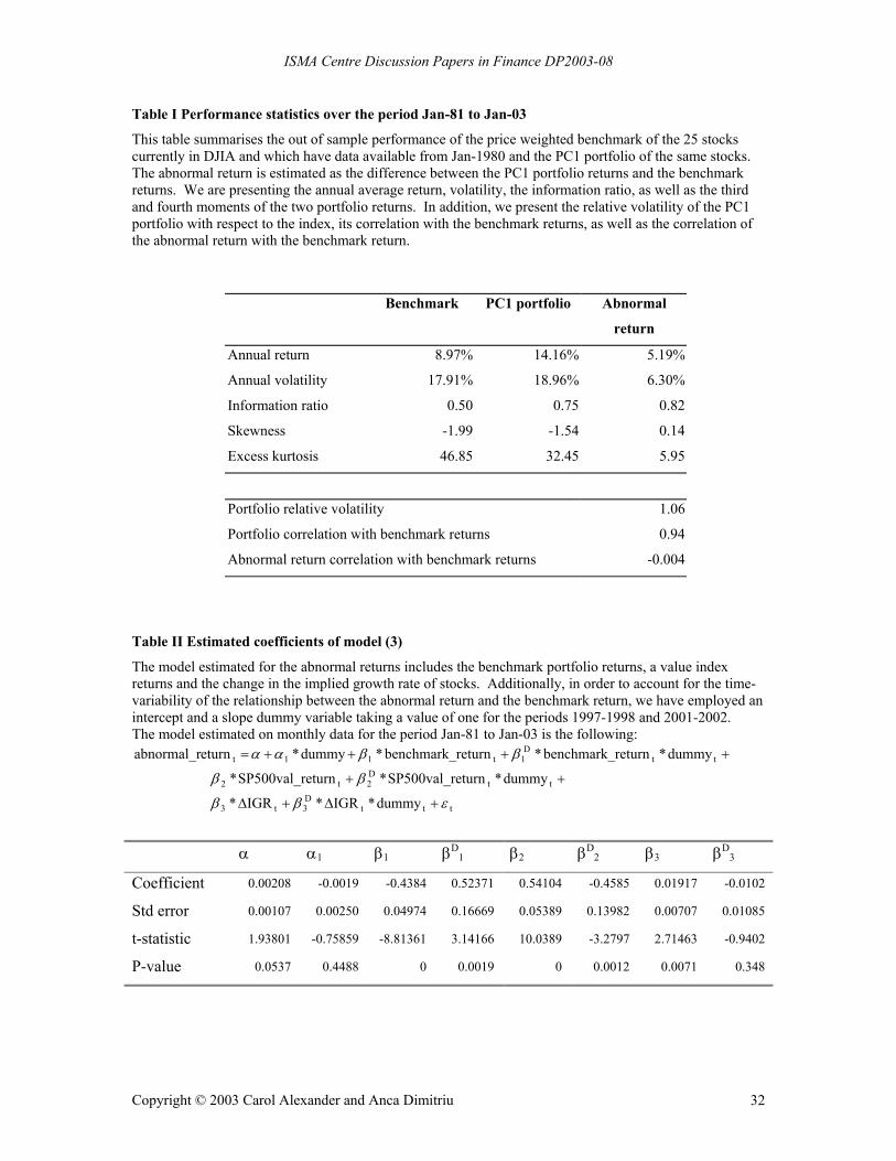
ISMA Centre Discussion Papers in Finance DP2003-08
Table I Performance statistics over the period Jan-81 to Jan-03
This table summarises the out of sample performance of the price weighted benchmark of the 25 stocks currently in DJIA and which have data available from Jan-1980 and the PC1 portfolio of the same stocks. The abnormal return is estimated as the difference between the PC1 portfolio returns and the benchmark returns. We are presenting the annual average return, volatility, the information ratio, as well as the third and fourth moments of the two portfolio returns. In addition, we present the relative volatility of the PC1 portfolio with respect to the index, its correlation with the benchmark returns, as well as the correlation of the abnormal return with the benchmark return.
Benchmark PC1 portfolio Abnormal
return
Annual return 8.97% 14.16% 5.19%
Annual volatility 17.91% 18.96% 6.30%
Information ratio 0.50 0.75 0.82
Skewness -1.99 -1.54 0.14
Excess kurtosis 46.85 32.45 5.95
Portfolio relative volatility 1.06
Portfolio correlation with benchmark returns 0.94
Abnormal return correlation with benchmark returns -0.004
Table II Estimated coefficients of model (3)
The model estimated for the abnormal returns includes the benchmark portfolio returns, a value index returns and the change in the implied growth rate of stocks. Additionally, in order to account for the time-variability of the relationship between the abnormal return and the benchmark return, we have employed an intercept and a slope dummy variable taking a value of one for the periods 1997-1998 and 2001-2002. The model estimated on monthly data for the period Jan-81 to Jan-03 is the following:
tttD3t3
ttD2t2
ttD
1t11t
dummy*IGR*IGR*
dummy*eturnSP500val_r* eturnSP500val_r*
dummy*returnbenchmark_*returnbenchmark_*dummy* eturnabnormal_r
εββ
ββ
ββαα
+∆+∆
++
++++=
α α1 β1 βD1 β2 βD
2 β3 βD3
Coefficient 0.00208 -0.0019 -0.4384 0.52371 0.54104 -0.4585 0.01917 -0.0102
Std error 0.00107 0.00250 0.04974 0.16669 0.05389 0.13982 0.00707 0.01085
t-statistic 1.93801 -0.75859 -8.81361 3.14166 10.0389 -3.2797 2.71463 -0.9402
P-value 0.0537 0.4488 0 0.0019 0 0.0012 0.0071 0.348
Copyright © 2003 Carol Alexander and Anca Dimitriu 32

ISMA Centre Discussion Papers in Finance DP2003-08
Appendix 1 We have ordered ascendingly the daily benchmark returns and split them in 10 groups with equal number of observations. The first group includes the worst 10% benchmark returns and the last one, the best 10% benchmark returns. We have then associated to each group the corresponding abnormal return of the PC1 portfolio. For each group, we have compute the average benchmark return and the corresponding average abnormal return, which are plotted in the graphs below, over different subsamples. Additionally, we report the first four moments of the PC1 portfolio, benchmark portfolio and abnormal return, together with the relative volatility of the PC1 portfolio, its correlation with the market returns and its beta. Jan-80 to Dec-89
Index Portfolio Xs returnAnnual return 12.51% 16.61% 4.11%Annual volatility 19.34% 19.48% 6.19%Skewness -3.61 -3.23 -0.11Excess kurtosis 80.90 65.10 2.39
Portfolio relative volatility 1.01Portfolio correlation with market returns 0.95Portfolio beta 0.96
Jan-90 to Dec-96
Index Portfolio Xs returnAnnual return 10.66% 16.58% 5.92%Annual volatility 13.30% 13.77% 5.96%Skewness -0.17 -0.07 0.95Excess kurtosis 3.80 2.77 11.52
Portfolio relative volatility 1.04Portfolio correlation with market returns 0.90Portfolio beta 0.94
Jan-97 to Dec-98
Index Portfolio Xs returnAnnual return 18.93% 22.48% 3.55%Annual volatility 18.92% 20.29% 4.81%Skewness -0.86 -0.59 0.18Excess kurtosis 7.33 5.13 0.85
Portfolio relative volatility 1.07Portfolio correlation with market returns 0.97Portfolio beta 1.04
Jan-99 to Dec-00
Index Portfolio Xs returnAnnual return -0.28% 16.28% 16.56%Annual volatility 18.36% 19.27% 7.49%Skewness -0.20 0.09 -0.02Excess kurtosis 1.40 1.34 2.60
Portfolio relative volatility 1.05Portfolio correlation with market returns 0.92Portfolio beta 0.97
Jan-01 to Feb-03
Index Portfolio Xs returnAnnual return -13.35% -15.21% -1.86%Annual volatility 22.86% 27.99% 7.65%Skewness 0.08 -0.04 -0.49Excess kurtosis 1.98 3.12 7.00
Portfolio relative volatility 1.22Portfolio correlation with market returns 0.97Portfolio beta 1.19
-3%
-2%
-1%
0%
1%
2%
3%
1 2 3 4 5 6 7 8 9 10
Index return10*xs return
-3%
-2%
-1%
0%
1%
2%
3%
1 2 3 4 5 6 7 8 9 10
Index return10*xs return
-3%
-2%
-1%
0%
1%
2%
3%
1 2 3 4 5 6 7 8 9 10
Index return10*xs return
-3%
-2%
-1%
0%
1%
2%
3%
1 2 3 4 5 6 7 8 9 10
Index return10*xs return
-6%
-4%
-2%
0%
2%
4%
6%
1 2 3 4 5 6 7 8 9 10
Index return10*xs return
Copyright © 2003 Carol Alexander and Anca Dimitriu 33
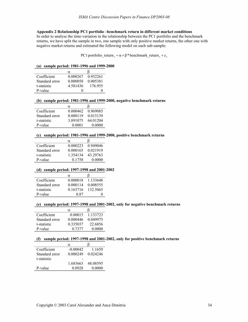
ISMA Centre Discussion Papers in Finance DP2003-08
Appendix 2 Relationship PC1 portfolio –benchmark return in different market conditions In order to analyse the time-variation in the relationship between the PC1 portfolio and the benchmark returns, we have split the sample in two, one sample with only positive market returns, the other one with negative market returns and estimated the following model on each sub-sample:
ttt returnbenchmark_*βα returnportfolio_ PC1 ε++= (a) sample period: 1981-1996 and 1999-2000 α β Coefficient 0.000267 0.952261 Standard error 0.000058 0.005381 t-statistic 4.581436 176.955 P-value 0 0 (b) sample period: 1981-1996 and 1999-2000, negative benchmark returns α β Coefficient 0.000462 0.969085 Standard error 0.000119 0.015139 t-statistic 3.891075 64.01204 P-value 0.0001 0.0000 (c) sample period: 1981-1996 and 1999-2000, positive benchmark returns α β Coefficient 0.000223 0.949046 Standard error 0.000165 0.021919 t-statistic 1.354134 43.29763 P-value 0.1758 0.0000 (d) sample period: 1997-1998 and 2001-2002 α β Coefficient 0.000018 1.133648 Standard error 0.000114 0.008555 t-statistic 0.163716 132.5065 P-value 0.87 0 (e) sample period: 1997-1998 and 2001-2002, only for negative benchmark returns α β
Coefficient 0.00015 1.133723 Standard error 0.000446 0.049975 t-statistic 0.335037 22.6856 P-value 0.7377 0.0000 (f) sample period: 1997-1998 and 2001-2002, only for positive benchmark returns α β Coefficient -0.00042 1.1659 Standard error 0.000249 0.024246 t-statistic -
1.683663 48.08595 P-value 0.0928 0.0000
Copyright © 2003 Carol Alexander and Anca Dimitriu 34

ISMA Centre Discussion Papers in Finance DP2003-08
Appendix 3 Description of the variables used in the factor model (source: www.barra.co.uk/research) Price/Earnings: the inverse of the capitalization-weighted average of the individual constituent Earnings/Price ratios. The individual company Earnings/Price ratio is the sum of the most recently available four quarters of income before extraordinary items divided by current company capitalization. Price/Book: the inverse of the capitalization-weighted average of the individual constituent Book/Price ratios. The individual company Book/Price ratio is the total common equity for the latest quarter divided by current company capitalization. Implied Dividend: dividend yield times index value, where the dividend yield is the capitalization-weighted average of the individual constituent indicated annual dividend yields. Return on Equity: the capitalization-weighted average of the individual constituent return on equity values. The individual company return on equity is the sum of the most recently available four quarters of income before extraordinary items divided by the average of the total common equity at the beginning and the end of the corresponding calculation year. Return on Assets: the capitalization-weighted average of the individual constituent return on assets values. The individual company return on assets is the sum of the most recently available four quarters of income before extraordinary items divided by the average of the total assets at the beginning and the end of the corresponding calculation year. Price/Sales: the inverse of the capitalization-weighted average of the individual constituent Sales/Price values. The individual company Sales/Price ratio is the sum of the most recently available four quarters of net sales divided by current company capitalization. Dividend Payout Ratio: the capitalization-weighted average of the individual constituent dividend payout ratios. The individual company payout ratio is the sum of the dividends paid during the previous four quarters divided by the sum of earnings for the previous four quarters. Price to Cash Flow: the inverse of the capitalization-weighted average of the individual constituent cash flow to price ratios. The individual company cash flow to price ratio is the sum of the last four quarters of depreciation and amortization, deferred taxes and net income before extraordinary items divided by the current market capitalization. Implied Growth Rate: the capitalization-weighted average of the individual constituent growth rates. The individual company growth rate is the 60 month average of the historical EPS growth, a function of return on equity and retention rate.
Copyright © 2003 Carol Alexander and Anca Dimitriu 35