VU University Amsterdam

Research Paper Business Analytics

The Bullwhip Effect: Analysis of theCauses and Remedies

Author:

Jonathan Moll

Supervisor:

Rene Bekker

VU University Amsterdam

Faculty of Sciences

Boelelaan 1081a

1081 HV Amsterdam

July 2013

Preface

This research paper is a compulsory part of the Master’s program Business Analytics at

the VU University Amsterdam. The student should do research on a business related

problem, with a strong mathematical or computer science component. The research

could be based on literature, but may also be extended with own research.

This research paper presents an elaborate literature overview of the bullwhip effect,

extended with computer simulations to get more insight in the processes that cause the

effect. The bullwhip effect is a phenomenon that refers to a trend of larger and larger

swings in inventory, as one moves upstream in a supply chain. Since a long crackling

whip is a suitable metaphor for the amplifying and oscillating swings in inventory, the

phenomenon is called the bullwhip effect.

I would like to thank Rene Bekker for the time and effort he spend supervising me.

Jonathan Moll

July 2013

iii

Summary

The bullwhip effect is a problem in supply chains that refers to amplifying swings in

inventory as one moves upstream along a supply chain (further away from the customer).

The aim of this paper is to give an elaborate literature overview, supplemented with

computer simulations to make the problem more intelligible.

In Chapter 2 we first describe the bullwhip effect based on the results of Sterman’s

beer game [22]. The beer game simulates a supply chain consisting of a beer retailer,

wholesaler, distributor and brewery. The game is played by four players who make

independent inventory decisions without consultation with other players. Typical game

results clearly demonstrate the amplification effects.

Secondly, we show how the bullwhip effect could be measured and present the simple

supply chain model of Chen et al. [6]. To quantify the size of the bullwhip effect, Chen

et al. propose the order rate variance ratio, which is given by the variance of the orders,

divided by the variance of the demand. If the ratio is greater than one, the bullwhip

effect exists.

Chen et al. assume that the demand follows an autoregressive model of the first degree,

an AR(1) model. They further assume that all members of the supply chain use a simple

order-up-to policy, where the mean demand and the average forecast error are estimated

with moving average forecasts. Given these assumptions, they derive a lower bound for

the order rate variance ratio. The ratio is always greater than one, which implies the

bullwhip effect.

To make the problem more intelligible we carry out two simulation experiments. We

first simulate a simple supply chain using exponential smoothing forecasting, and then

simulate the model of Chen et al. The simulation results clearly show the amplifying

swings in demand and inventory as one moves upstream the supply chain. It also shows

the high levels of safety stock that are needed to compensate for the large swings in

inventory. The order rate variance ratio grows fast if the lead time between ordering

and receiving grows. The impact of the degree of serial correlation of the demand is also

significant. If the correlation parameter increases, then the order rate variance ratio will

decrease.

v

vi

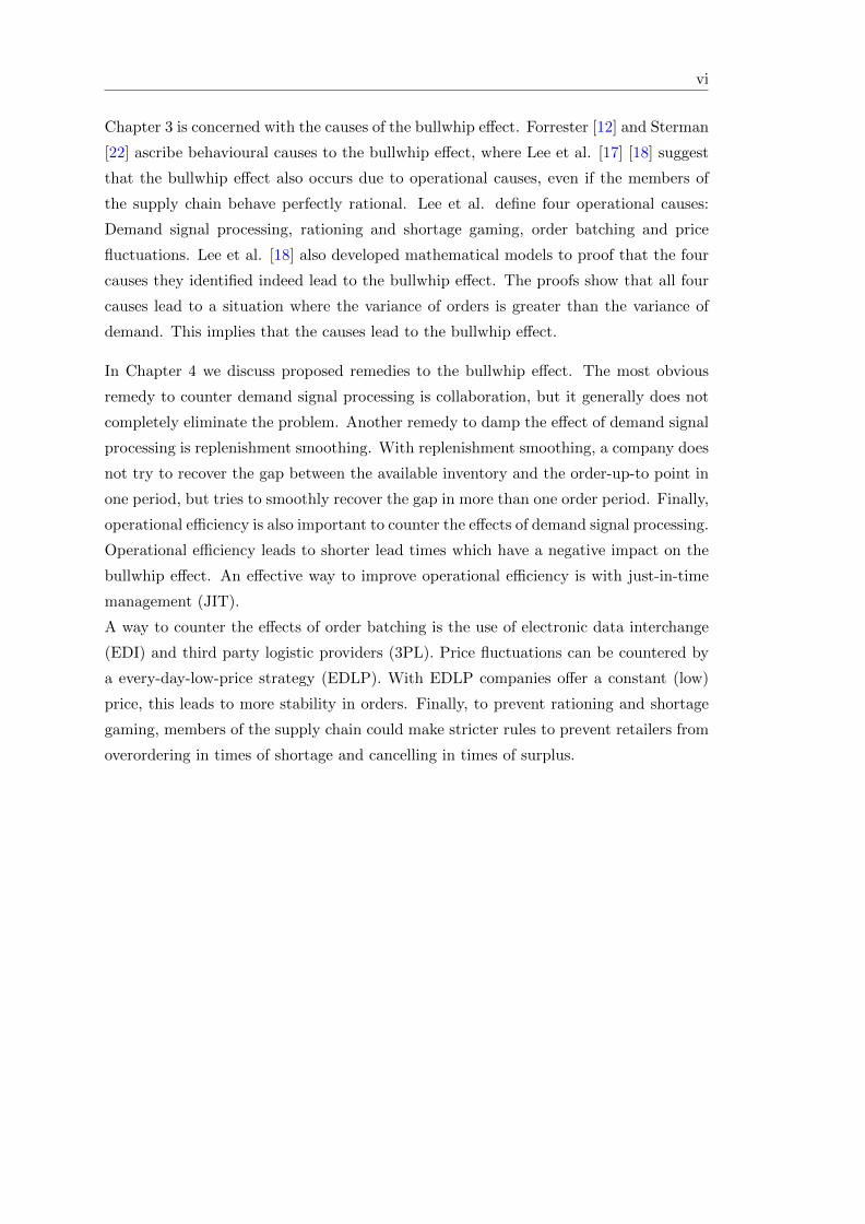
Chapter 3 is concerned with the causes of the bullwhip effect. Forrester [12] and Sterman

[22] ascribe behavioural causes to the bullwhip effect, where Lee et al. [17] [18] suggest

that the bullwhip effect also occurs due to operational causes, even if the members of

the supply chain behave perfectly rational. Lee et al. define four operational causes:

Demand signal processing, rationing and shortage gaming, order batching and price

fluctuations. Lee et al. [18] also developed mathematical models to proof that the four

causes they identified indeed lead to the bullwhip effect. The proofs show that all four

causes lead to a situation where the variance of orders is greater than the variance of

demand. This implies that the causes lead to the bullwhip effect.

In Chapter 4 we discuss proposed remedies to the bullwhip effect. The most obvious

remedy to counter demand signal processing is collaboration, but it generally does not

completely eliminate the problem. Another remedy to damp the effect of demand signal

processing is replenishment smoothing. With replenishment smoothing, a company does

not try to recover the gap between the available inventory and the order-up-to point in

one period, but tries to smoothly recover the gap in more than one order period. Finally,

operational efficiency is also important to counter the effects of demand signal processing.

Operational efficiency leads to shorter lead times which have a negative impact on the

bullwhip effect. An effective way to improve operational efficiency is with just-in-time

management (JIT).

A way to counter the effects of order batching is the use of electronic data interchange

(EDI) and third party logistic providers (3PL). Price fluctuations can be countered by

a every-day-low-price strategy (EDLP). With EDLP companies offer a constant (low)

price, this leads to more stability in orders. Finally, to prevent rationing and shortage

gaming, members of the supply chain could make stricter rules to prevent retailers from

overordering in times of shortage and cancelling in times of surplus.

Contents

Preface ii

Summary iv

1 Introduction 1

2 The Bullwhip Effect 3

2.1 Description of the Phenomenon . . . . . . . . . . . . . . . . . . . . . . . . 3

2.2 Measurement and Quantitative Analysis . . . . . . . . . . . . . . . . . . 4

2.2.1 A Simple Supply Chain Model . . . . . . . . . . . . . . . . . . . . 5

2.3 Simulation Experiments . . . . . . . . . . . . . . . . . . . . . . . . . . . . 9

2.3.1 Simulation with Exponential Smoothing Forecasting . . . . . . . . 9

2.3.2 Simulation With Moving Average Forecasting . . . . . . . . . . . . 13

3 Causes of the Bullwhip Effect 15

3.1 Behavioural Causes . . . . . . . . . . . . . . . . . . . . . . . . . . . . . . . 15

3.2 Operational Causes . . . . . . . . . . . . . . . . . . . . . . . . . . . . . . . 16

3.2.1 Demand Signal Processing . . . . . . . . . . . . . . . . . . . . . . . 16

3.2.2 Order Batching . . . . . . . . . . . . . . . . . . . . . . . . . . . . . 20

3.2.3 Price Fluctuation . . . . . . . . . . . . . . . . . . . . . . . . . . . . 24

3.2.4 Rationing and Shortage Gaming . . . . . . . . . . . . . . . . . . . 27

4 Remedies to the Bullwhip Effect 31

4.1 Remedies to Demand Signal Processing . . . . . . . . . . . . . . . . . . . 31

4.1.1 Collaboration . . . . . . . . . . . . . . . . . . . . . . . . . . . . . . 31

4.1.2 Replenishment smoothing . . . . . . . . . . . . . . . . . . . . . . . 33

4.1.3 Operational Efficiency . . . . . . . . . . . . . . . . . . . . . . . . . 34

4.2 Remedies to Order Batching . . . . . . . . . . . . . . . . . . . . . . . . . . 34

4.3 Remedies to Price Fluctation . . . . . . . . . . . . . . . . . . . . . . . . . 35

4.4 Remedies to Rationing and Shortage Gaming . . . . . . . . . . . . . . . . 35

5 Conclusion and Discussion 37

Bibliography 39

vii

Chapter 1

Introduction

A key issue in supply chain management is the control of inventory. Members of a supply

chain adopt policies and operating procedures to optimize their use of inventory such

that it minimizes their investments in inventory while keeping high customer service

levels. Uncertainty is inherent to every supply chain through factors such as variability

in demand, lead times, breakdowns of machines and local politics. Because uncertainty

is given, companies often carry an inventory buffer called safety stock. An important ob-

servation in supply chain management is that small variations in demand from customers

result in increasingly large variations in demand as one moves up the supply chain (fur-

ther away from the customer). This phenomenon is known as the bullwhip effect. The

bullwhip effect can lead to major inefficiencies such as excessive inventory investments,

high levels of safety stock, misguided capacity plans, inactive transportation and poor

customer service.

The bullwhip effect has been noted across a range of academic disciplines, which as-

signed various causes and proposed differing remedies for the problem. The effect of de-

mand amplification upstream in a supply chain was first described in 1961 by Forrester

[12], who used computer simulation to show the existence of demand amplification and

demonstrated its effects. Forrester’s fundamental explanation was that it is primarily a

function of decision making in response to variability in incoming demand. Forrester’s

remedy lay in understanding the system as a whole, and modelling that system with

specific simulation models, so that managers can determine appropriate action.

Perhaps the most well-known description of the bullwhip effect has come from Sterman

[22] in 1989. Sterman illustrates the bullwhip effect with the “beer distribution game”

that simulates a supply chain consisting of a beer retailer, wholesaler, distributor and

brewery. The game is played by four players who make independent inventory decisions

without consultation with other players. The individual players only rely on the orders

1

Chapter 1. Introduction 2

of the neighbouring player. Again, the amplification effects were clearly demonstrated.

Sterman interprets the phenomenon as a consequence of players’ systematic irrational

behaviour, or “misperceptions of feedback”.

In contradiction to Forrester [12] and Sterman [22], who ascribed the bullwhip effect to

irrational behaviour of managers, Lee et al. [17] identify in 1997 four operational causes

of the bullwhip effect: Demand signal processing, rationing gaming, order batching, and

price discounting. These four high level causes have become the standard for this phe-

nomenon. In the same year, Lee et al. [18] employ mathematical models to demonstrate

how these causes can lead, even with rational decision making, to the amplification of

demand. Since these papers, much research has been done on the impact of different

methods to counter the causes of the bullwhip effect. Some examples are Chen et al.

[6], Cachon et al. [3], Disney et al. [8], Canella et al. [4].

This first aim of this paper is to give an extensive literature overview of the bullwhip

effect, its causes and proposed remedies. Secondly, it illustrates the bullwhip effect and

the impact of different parameters on the bullwhip effect in simulation experiments.

In Chapter 2 we first describe the bullwhip effect based on the results of Sterman’s beer

game [22]. Then we show how the bullwhip effect can be measured and present the

simple supply chain model of Chen et al. [6]. Finally, in the last section of Chapter 2,

we carry out simulation experiments to gain more insight in the process that causes the

bullwhip effect. Chapter 3 is concerned with the causes of the bullwhip effect. First we

describe the behavioural causes advocated by Forrester [12] and Sterman [22]. Then we

give an extensive description and present the mathematical proofs for the operational

causes identified by Lee et al. [17] [18]. In the last chapter we describe proposed remedies

to counter the four operational causes identified by Lee et al. [17]. We conclude with a

short discussion about the literature.

Chapter 2

The Bullwhip Effect

Consider multiple companies operating in a serial supply chain, each of whom orders

from its immediate upstream neighbour. Research indicates that small variations in

demand from customers result in increasingly large variations as demand is transmitted

upstream along the supply chain. In this chapter we first give a description of this

phenomenon on the basis of the “beer distribution game” from Sterman [22]. Secondly,

we give an introduction to the measurement and quantitative analysis of the bullwhip

effect on the basis of a simple supply chain model, developed by Chen et al. [6]. In

the last section we do simulation experiments to gain more insight in the process that

causes the bullwhip effect and to study the impact of different parameters on the size of

the effect.

2.1 Description of the Phenomenon

Probably the most well known demonstration of the bullwhip effect was carried out by

Sterman [22] with the well known “beer distribution game”. The game is a role-playing

simulation that portrays the supply chain of beer. It consists of four sectors: retailer,

wholesaler, distributor and factory. The game is played in teams of four persons and each

person manages one sector. Each week a card is drawn that represents customer demand.

The retailer ships the beer requested out of its inventory and orders new beer from the

wholesaler, who ships the beer requested out of its inventory and orders beer from the

distributor, who orders and receives beer from the factory. So there is a downstream

flow of physical goods and an upstream flow of demand information, as displayed in

Figure 2.1. At each stage there are order and receiving delays that represent the time

required to receive, process, ship, and deliver orders. The objective is to minimize total

company costs that consists of inventory holding costs and stockout costs.

3

Chapter 2. The Bullwhip Effect 4

Figure 2.1: From Metters [19]. Flow of goods and information in the beergame.

The game has been played all over the world by thousands of people ranging from high

school students to chief executive officers and government officials. All of these trials

show the following results. Orders and inventory are both subject to instability and

oscillation. In almost all cases, the inventory levels of the retailer decline, followed by a

decline in inventory of the wholesaler, distributor and factory. As inventory falls, players

tend to increase their orders. As additional beer is brewed, inventory levels grow and in

many cases overshoot the desired level. As a reaction, orders fall of rapidly. In addition,

the amplitude and variance of orders increases as one moves from retailer to factory and

the order rate tends to peak later at each stage. Figure 2.2 shows the effects in four

typical trials. The oscillation, amplification and phase lag effects are clearly visible.

The bullwhip effect is not solely observed in theory and simulations, it has been rec-

ognized in many markets. Procter & Gamble (P&G) found strange order patterns for

diapers. The sales at retail stores were fluctuating, but the fluctuations were relatively

small compared to the large variability of orders placed by the distributor. The distrib-

utors orders to their suppliers were even larger. This did not make sense, because the

babies consumed diapers at a steady rate, whereas the variations in demand were am-

plified as they moved up the supply chain. P&G called this phenomenon the bullwhip

effect. The same phenomenon was observed by executives of Hewlett-Packard in the

supply chain for laser printers [17]. Also many examples can be found in the grocery

industry [1], and automotive industry [2].

2.2 Measurement and Quantitative Analysis

Measurement and quantitative analysis of the bullwhip effect is of great importance for

both theoretical and empirical purposes. The most common measure to quantify the

bullwhip effect is the order rate variance ratio. This measure was proposed by Chen et

Chapter 2. The Bullwhip Effect 5

Figure 2.2: From Sterman [22]. Top: orders. Bottom: inventory. From bottom totop: retailer, wholesaler, distributor, factory.

al. [6] and is defined as the ratio of the variance of placed orders and observed customer

demand. The larger the order rate variance ratio, the stronger the bullwhip effect. In

the same paper Chen et al. use a simple supply chain model to extract a lower bound

on the order rate variance ratio at each stage of the supply chain. A description of this

model and a summary of the results are given below.

2.2.1 A Simple Supply Chain Model

Consider a simple supply chain in which in each period t, a single retailer observes its

inventory level and places an order qt to a single manufacturer. The observed demand

at the end of period t is denoted by Dt. There is a fixed lead time of L periods between

the time an order is placed by the retailer and the time the order is received from the

manufacturer. The observed demand is assumed to be of the form

Dt = µ+ ρDt−1 + εt, (2.1)

where µ is a non-negative constant, ρ is a correlation parameter with |ρ| < 1, and the

error terms, εt, are independent and identically distributed (i.i.d) from a symmetric

Chapter 2. The Bullwhip Effect 6

distribution with mean 0 and variance σ2. The demand process (2.1) is known as a

first-order autoregressive model (AR(1) model). The expectation and variance of Dt

can easily be derived.

E[Dt] = E[µ] + ρE[Dt−1] + E[εt] = µ+ ρµ,

so

E[Dt] =µ

1− ρ. (2.2)

For the variance it holds that

V ar(Dt) = V ar(µ) + ρ2V ar(Dt−1) + V ar(εt) = ρ2V ar(Dt−1) + σ2.

Because |ρ| < 1, V ar(Dt) becomes independent of t, and hence

V ar(Dt) =σ2

(1− ρ)2. (2.3)

The Inventory Policy and Forecasting Technique

Chen et al. [6] assume that the retailer follows a simple order-up-to inventory policy in

which the order-up-to point yt is estimated from the observed demand as

yt = D̂Lt + zσ̂Let, (2.4)

where D̂Lt is an estimate of the mean lead time demand in period t, σ̂Let is an estimate

of the standard deviation of the L period forecast error in period t, and z is a constant

chosen to meet a desired service level.

To estimate D̂Lt and σ̂Let Chen et al. assume that the retailer uses a simple moving

average based on the demand observation from the previous p periods. That is,

D̂Lt = L

(∑pi=1Dt−ip

), (2.5)

and

σ̂Let = CL,ρ

√∑pi=1(et−i)

2

p, (2.6)

where et−i is the forecast error in period t − i and CL,ρ is a constant function of L, ρ

and p. For details about this constant, the reader is referred to Ryan [20]. The use of a

simple moving average for the estimaters D̂Lt and σ̂Let is in general not optimal. However,

this method is often used in practice and is therefore a realistic choice.

Chapter 2. The Bullwhip Effect 7

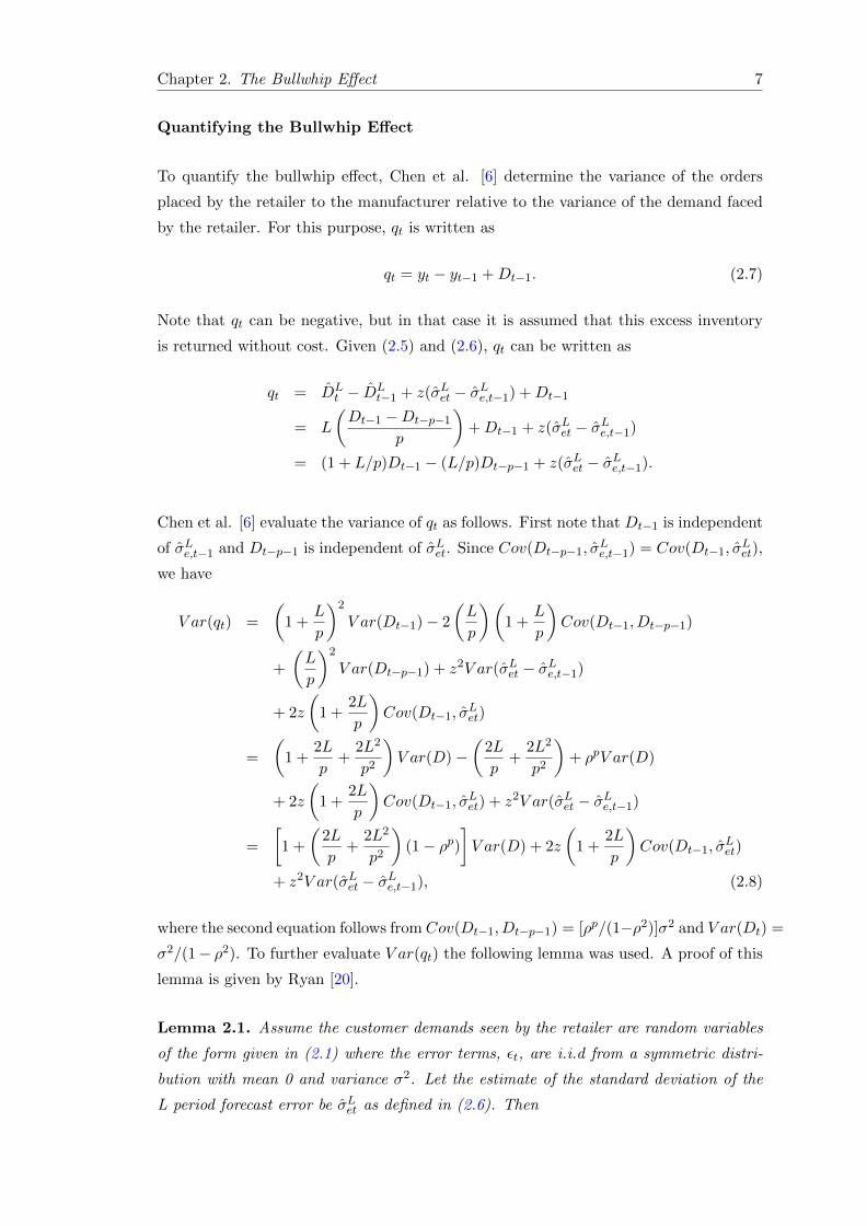
Quantifying the Bullwhip Effect

To quantify the bullwhip effect, Chen et al. [6] determine the variance of the orders

placed by the retailer to the manufacturer relative to the variance of the demand faced

by the retailer. For this purpose, qt is written as

qt = yt − yt−1 +Dt−1. (2.7)

Note that qt can be negative, but in that case it is assumed that this excess inventory

is returned without cost. Given (2.5) and (2.6), qt can be written as

qt = D̂Lt − D̂L

t−1 + z(σ̂Let − σ̂Le,t−1) +Dt−1

= L

(Dt−1 −Dt−p−1

p

)+Dt−1 + z(σ̂Let − σ̂Le,t−1)

= (1 + L/p)Dt−1 − (L/p)Dt−p−1 + z(σ̂Let − σ̂Le,t−1).

Chen et al. [6] evaluate the variance of qt as follows. First note that Dt−1 is independent

of σ̂Le,t−1 and Dt−p−1 is independent of σ̂Let. Since Cov(Dt−p−1, σ̂Le,t−1) = Cov(Dt−1, σ̂

Let),

we have

V ar(qt) =

(1 +

L

p

)2

V ar(Dt−1)− 2

(L

p

)(1 +

L

p

)Cov(Dt−1, Dt−p−1)

+

(L

p

)2

V ar(Dt−p−1) + z2V ar(σ̂Let − σ̂Le,t−1)

+ 2z

(1 +

2L

p

)Cov(Dt−1, σ̂

Let)

=

(1 +

2L

p+

2L2

p2

)V ar(D)−

(2L

p+

2L2

p2

)+ ρpV ar(D)

+ 2z

(1 +

2L

p

)Cov(Dt−1, σ̂

Let) + z2V ar(σ̂Let − σ̂Le,t−1)

=

[1 +

(2L

p+

2L2

p2

)(1− ρp)

]V ar(D) + 2z

(1 +

2L

p

)Cov(Dt−1, σ̂

Let)

+ z2V ar(σ̂Let − σ̂Le,t−1), (2.8)

where the second equation follows from Cov(Dt−1, Dt−p−1) = [ρp/(1−ρ2)]σ2 and V ar(Dt) =

σ2/(1− ρ2). To further evaluate V ar(qt) the following lemma was used. A proof of this

lemma is given by Ryan [20].

Lemma 2.1. Assume the customer demands seen by the retailer are random variables

of the form given in (2.1) where the error terms, εt, are i.i.d from a symmetric distri-

bution with mean 0 and variance σ2. Let the estimate of the standard deviation of the

L period forecast error be σ̂Let as defined in (2.6). Then

Chapter 2. The Bullwhip Effect 8

Cov(Dt−i, σ̂Let) = 0 for all i = 1, . . . , p.

By rewriting Equation (2.8) using Lemma 2.1, Chen et al. [6] found the following lower

bound on the increase in variability from the retailer to the manufacturer.

V ar(q)

V ar(D)≥ 1 +

(2L

p+

2L2

p2

)(1− ρp). (2.9)

When z = 0, the bound is tight.

Interpretation of the Results

Several observations can be made from (2.9). First, since L ≥ 1, the increase in vari-

ability of orders from the retailer to the manufacturer is greater than one, and thus the

bullwhip effect occurs. If 0 ≤ ρ ≤ 1, the ratio is a decreasing function of p, a decreasing

or alternating function of ρ, and an increasing function of L. The number of observations

p used to estimate the mean and variance of demand have a significant impact. Note

that if p becomes large, the lower bound becomes one. However, because (2.9) gives

only a lower bound, it is not necessarily true that the bullwhip effect will not occur with

perfectly accurate estimates.

A remarkable fact is that if ρ < 0, then ρp is alternating, which suggests that the increase

in variability will be larger for odd values of p than for even values of p. This is logical,

because if ρ is negative, the demand is alternating and the estimation of the mean

and variance will be more accurate after an even number of observations. For example,

suppose that if you estimate from three data points, you estimate from two high numbers

and one low number. This will lead to a high estimate for the next number, while it

will be low because of the negative correlation. In contrast, if you would estimate from

four data points, you will estimate from two high numbers and two low numbers. Your

estimate will be in the middle, which will give a more accurate estimate than with three

data points.

Chen et al. [6] do not say anything about the impact of the customer service level

parameter z on the order rate variance ratio. The customer service level z does not

appear in the lower bound. It only appears in the exact equation for the order rate

variance ratio, which can easily be derived from (2.8), using Lemma 2.1.

V ar(q)

V ar(D)= 1 +

(2L

p+

2L2

p2

)(1− ρp) +

z2V ar(σ̂Let − σ̂Le,t−1)V ar(D)

. (2.10)

Chapter 2. The Bullwhip Effect 9

From (2.10) can be observed that the order rate variance ratio becomes higher when a

higher z is chosen. However, the exact behaviour of the last term of (2.10) stays unclear,

because V ar(σ̂Let− σ̂Le,t−1) is unknown and depends on the other parameters. It would be

interesting to know a bit more about this term. In the next section we do a spreadsheet

simulation with Crystal Ball where we study ‘among others’ the behaviour of the last

term of (2.10).

2.3 Simulation Experiments

In this section we simulate the supply chain of the beer game using Excel with Crystal

Ball. First, we simulate the process with exponential smoothing forecasting, a method

that is often used in practice. Secondly, we simulate the simple supply chain model of

the previous section to study the behaviour of the order rate variance ratio and compare

the simulation results with the analytical results derived by Chen et al. [6].

2.3.1 Simulation with Exponential Smoothing Forecasting

Consider a supply chain in which all members observe their inventory at the beginning

of each week and place an order to their upstream neighbour based on their observation.

We assume that the demands seen by the retailer follow the AR(1) model of (2.1). There

is a fixed lead time of L weeks and any unfilled orders are backlogged. We assume further

that all members of the supply chain use a simple order-up-to policy, where the order-

up-to point yt is estimated from the observed demand as in Equation (2.4). Suppose

that the retailer, wholesaler, manufacturer and supplier use exponential smoothing to

forecast the mean demand. The mean lead time demand is in then estimated by

D̂Lt = L(αDt−1 + (1− α)D̂t−1). (2.11)

To estimate the standard deviation of the forecast error we use the square root of the

sample variance of the forecast error based on one year of simulated historical data.

The inventory policy and forecasting technique described above are not necessarily opti-

mal. However, such policies are commonly used in practice and give a good impression

of how the bullwhip effect can occur.

Figure 2.3 shows the effects of the policy described above in a typical simulation run. The

bullwhip effect is clearly present. In the figure you see that the variance of the orders

become greater at each stage further upstream the supply chain. Also the inventory

levels contain larger and larger swings at each stage. Consequently, high levels of safety

Chapter 2. The Bullwhip Effect 10

stock are needed. The graphs of Figure 2.3 look different from the graphs presented by

Sterman, see Figure 2.2. The effects shown by Sterman look more extreme than our

simulation results. This is probably because behavioural causes of the bullwhip effect

are not present in our simulation. Members of the supply chain order strictly consistent

with an order-up-to policy, where players of the beergame react more directly to demand

signals from their upstream neighbours.

Figure 2.3: Simulation of the supply chain model with exponential smoothing.µ = 10, ρ = 0.3, σ = 2, L = 2 , z = 2, α = 0.3

To study the impact of the different parameters of the model, we simulate the model to

Chapter 2. The Bullwhip Effect 11

forecast the order rate variance ratio (ORVR) at the retailer under different parameter

values. The order rate variance ratio is given by the variance of the orders divided by

the variance of the demand. We only study the situation at the retailer, because the

ratio is stable at each stage of the supply chain, so the results will be the same at other

links in the supply chain. For each parameter, we vary the value of the parameter,

while keeping the other parameters constant. We use the parameter setting of Figure

2.3 as basic setting. Figure 2.4 shows the impact of the different parameters on the

order rate variance ratio. The forecasts are based on 1000 simulation runs, where in

each simulation run the order rate variance ratio is estimated from 2 year of data.

Figure 2.4: The impact of different parameters on the order rate variance ratio.

Several observations can be made regarding the impact of the different parameters as

shown in Figure 2.4. It must be noted, that the effects of the parameters on the order

rate variance ratio are subject to the inventory policy and forecast technique, so they

do not have to hold in general.

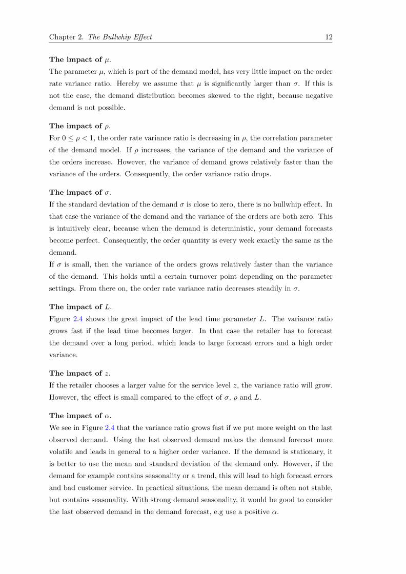
Chapter 2. The Bullwhip Effect 12

The impact of µ.

The parameter µ, which is part of the demand model, has very little impact on the order

rate variance ratio. Hereby we assume that µ is significantly larger than σ. If this is

not the case, the demand distribution becomes skewed to the right, because negative

demand is not possible.

The impact of ρ.

For 0 ≤ ρ < 1, the order rate variance ratio is decreasing in ρ, the correlation parameter

of the demand model. If ρ increases, the variance of the demand and the variance of

the orders increase. However, the variance of demand grows relatively faster than the

variance of the orders. Consequently, the order variance ratio drops.

The impact of σ.

If the standard deviation of the demand σ is close to zero, there is no bullwhip effect. In

that case the variance of the demand and the variance of the orders are both zero. This

is intuitively clear, because when the demand is deterministic, your demand forecasts

become perfect. Consequently, the order quantity is every week exactly the same as the

demand.

If σ is small, then the variance of the orders grows relatively faster than the variance

of the demand. This holds until a certain turnover point depending on the parameter

settings. From there on, the order rate variance ratio decreases steadily in σ.

The impact of L.

Figure 2.4 shows the great impact of the lead time parameter L. The variance ratio

grows fast if the lead time becomes larger. In that case the retailer has to forecast

the demand over a long period, which leads to large forecast errors and a high order

variance.

The impact of z.

If the retailer chooses a larger value for the service level z, the variance ratio will grow.

However, the effect is small compared to the effect of σ, ρ and L.

The impact of α.

We see in Figure 2.4 that the variance ratio grows fast if we put more weight on the last

observed demand. Using the last observed demand makes the demand forecast more

volatile and leads in general to a higher order variance. If the demand is stationary, it

is better to use the mean and standard deviation of the demand only. However, if the

demand for example contains seasonality or a trend, this will lead to high forecast errors

and bad customer service. In practical situations, the mean demand is often not stable,

but contains seasonality. With strong demand seasonality, it would be good to consider

the last observed demand in the demand forecast, e.g use a positive α.

Chapter 2. The Bullwhip Effect 13

2.3.2 Simulation With Moving Average Forecasting

In this section we simulate the simple supply chain model of Chen et al. [6]., described

in Section 2.2. The difference with the previous paragraph is that we now use moving

average forecasting, instead of exponential smoothing. Chen et al. use a simple supply

chain model to derive a lower bound on the order rate variance ratio (2.9). The lower

bound shows that the bullwhip effect exists, but the size of the effect stays unclear. In

this simulation experiment we forecast the order rate variance and use it to calculate the

fraction of the variance ratio that is contributed by the last term of Equation (2.10). In

the experiments we each time vary one parameter while keeping the other parameters

constant. As basic setting we use µ = 10, ρ = 0.3, σ = 2, L = 2, z = 2, p = 20. The

results are shown in Figure 2.5.

Figure 2.5: The impact of different parameters on the last term of Equation (2.10)

Chapter 2. The Bullwhip Effect 14

The red line in Figure 2.5 shows the absolute value of the last term of Equation (2.10).

The blue line is the fraction of this rest term compared to the total size of the order

rate variance ratio. We see that in most cases the rest term is smaller than 10% of the

variance ratio. However, the rest term starts to grow significantly as σ decreases or if L

increases. If σ decreases, the variance of the demand will be smaller and therefore the

rest term will be smaller too. If the lead time L becomes larger, then it becomes more

difficult to estimate the lead time demand and the mutual differences in forecasts will

be larger. Consequently, the numerator of the rest term will grow.

Chapter 3

Causes of the Bullwhip Effect

Originally, the bullwhip effect was ascribed mainly to the irrational behaviour of individ-

uals. Forrester [12] and Sterman [22] both assigned behavioural causes to the bullwhip

effect. Later, since Lee et al. [17], much research focused on operational causes of

the phenomenon. Lee et al [17] identified four high level causes of the bullwhip effect:

demand signal processing, rationing and shortage gaming, order batching and price fluc-

tuation. These causes have been widely accepted as a complete explanation for the

bullwhip effect. However, as Sterman [22] showed, behaviour and irrational decision

making of individual managers can have a significant impact on the bullwhip effect.

This chapter first gives a description of the behavioural causes as suggested by Forrester

and Sterman. Secondly, it gives an elaborate description of the four operational causes

identified by Lee et al. ([17],[18]) and how these causes can lead to the bullwhip effect.

3.1 Behavioural Causes

Forrester suggested that the decision logic of the individuals that are responsible for

demand management creates a tendency to over-respond to increases or decreases in

demand from customers in terms of orders placed on the immediate upstream neigh-

bours. If customer demand increases, demand to the upstream neighbour is increased to

meet the increase of customer demand. Demand to the upstream neighbour is further

increased to replenish inventory, which was depleted by the initial increase of customer

demand. The same exaggerated effects can occur if customer demand drops. Next to

that, the time lags in the transmission of both order information and materials along

the supply chain can exacerbate the effect. Buffa and Miller (1979) illustrated this with

the following example. Imagine a product with constant deterministic demand that is

delivered through the supply chain of the beergame, depicted in Figure 2.1. The retailer

15

Chapter 3. Causes of the Bullwhip Effect 16

sees a permanent 10% drop in sales on day 1, but consistent with a reorder point policy,

does not place an order until say day 10. Accordingly, the wholesaler notes the 10%

decrease on day 10, but does not place an order until day 20. As this process moves up

the supply chain, the firm furthest upstream may not discover the decline in demand

for several weeks. However, during this time they are producing at the old rate, which

is 1/0.9 = 111% of the new consumer requirement. Consequently, excess production of

11% per day would have accumulated since day 1. Due to the overstock position, pro-

duction may be cut back substantially more than 10%, which is an exaggerated reaction

to the actual demand decrease.

Sterman [22] also identified a number of behavioural causes of the bullwhip effect. First,

members of the supply chain do not adequately account for the delays between order

placement and order delivery. These misperceptions of time lags lead to continued over

and under ordering in the intervening periods. Moreover, members of the supply chain

do not use optimal stock levels and only try to optimise their own element of the chain.

3.2 Operational Causes

Lee et al. ([17], [18]) showed that the bullwhip effect is not solely a result of irrational

decision making, but a consequence of the players rational behaviour within the supply

chain’s infrastructure. Lee et al. [17] identified four high level causes of the bullwhip

effect:

1. Demand signal processing

2. Order batching

3. Price fluctuation

4. Rationing and shortage gaming

These four causes have become the standard and are widely accepted as a framework for

classifying all causes of the bullwhip effect. In this section we describe these for causes

and present the mathematical proofs of Lee et al. [18] that these causes indeed lead to

the bullwhip effect.

3.2.1 Demand Signal Processing

The product forecasting in the “beer game setting” is based on the order history from

the company’s immediate downstream neighbour. Each player in the beer game usually

Chapter 3. Causes of the Bullwhip Effect 17

acts on the demand signals that he or she observes. When a downstream operation

places an order, the upstream manager processes that piece of information as a signal

about future product demand. Based on this signal, the upstream manager readjust his

or her demand forecast. This is what Lee et al. [17] call demand signal processing.

For example, suppose that a manager uses exponential smoothing to determine how

much to order from a supplier. Exponential smoothing is commonly used in practice.

It is a forecast technique whereby demands are continuously updated as the new daily

demand data become available. The forecasts of future demands and associated safety

stocks are updated using the smoothing technique. With long lead times, it is not

uncommon to have high levels of safety stocks. The fluctuations in order quantities

can therefore be much greater than those in demand data. Now, suppose the upstream

neighbour in the supply chain also uses exponential smoothing and uses the orders to

forecast the demand. The orders that are placed by this neighbour will have even bigger

swings, see Figure 3.1.

Figure 3.1: From Lee et al. [17]. Higher variability in orders from retailer to manu-facturer than actual sales.

It is intuitively clear that longer lead times lead to greater fluctuations. As explained

above, safety stock contributes to the bullwhip effect. With longer lead times the need

for safety stock will be greater.

The reasoning above leads to the hypotheses that the variance of retail orders is strictly

larger than that of retail sales and the larger the replenishment lead time, the larger

Chapter 3. Causes of the Bullwhip Effect 18

the variance of orders. Lee et al. [18] give a mathematical proof of the hypotheses. A

summary is given below.

Mathematical Approach

Consider a multi-period inventory model. Lee et al. [18] assume serially correlated

demands which follow the process

Dt = d+ ρDt−1 + µt (3.1)

where Dt is the demand in period t, ρ is a correlation parameter satisfying 0 < ρ < 1

and µt is independent and identically normally distributed with zero mean and variance

σ2. Note that this is a different notation for a similar demand model as used by Chen et

al. [6], described in Chapter 1, see Equation (2.1). The only difference is the assumption

that µt is normally distributed, instead of symmetrically distributed.

The retailer orders a quantity zt from a supplier each period t. There is a delay of

v periods between ordering and receiving the goods, representing the order lead time

and the transit time from the supplier to the retailer’s site. It is assumed that excess

inventory can be returned without cost. Let h, π and c denote the unit holding cost,

the unit shortage penalty cost and the unit ordering cost, respectively. St is the amount

in stock plus on order (including those in transit). Let β be the cost discount factor

per period. The cost-minimization problem in an arbitrary period (normalized at 1) is

formulated as

minSt

[ ∞∑t=1

βt−1E1

[czt + βvg

(St,

t+v∑i=t

Di

)]], (3.2)

where

g

(St,

t+v∑i=t

Di

)= h

(St −

t+v∑i=t

Di

)+

+ π

(t+v∑i=t

Di − St

)+

.

See Heyman et al. [13] for its derivation. The expectation operator E1 denotes the ex-

pectation taken at the decision point of period 1, conditional on the demand realizations

Di, i = 0,−1,−2, . . ..

Theorem 3.1. In the setting of (3.2), we have:

(a) if 0 < ρ < 1, the variance of retail orders is strictly larger than that of retail sales;

i.e, V ar(z1) > V ar(D0).

(b) if 0 < ρ < 1, the larger the replenishment lead time, the larger the variance of orders;

i.e., V ar(z1) strictly increases in v.

Chapter 3. Causes of the Bullwhip Effect 19

Proof. (From Lee et al. [18])

Heyman et al. [13] showed that the minimization problem of Equation (3.2) can be

solved by solving

minSt

∞∑t=1

βt−1E1 [G(St)] ,

where G(S) = c(1− β)S + βvE1

[g(S,∑v+1

i=1 Di

)]. Also, they show that

S∗1 = Q−1v+1

[π − c(1− β)/βv

h+ π

], (3.3)

where Qv+1 denotes the distribution function of∑v+1

i=1 Di.

Now note that

Dk = d+ ρDk−1 + µk

= d(1 + ρ) + ρ2Dk−2 + (ρµk−1 + µk)

= . . .

= d1− ρk

1− ρ+ ρkD0 +

k∑i=1

ρk−iµi for k ≥ 1.

Thus∑v+1

i=1 Di at the decision point in period 1 is a N(M,Σ) distributed random variable

with

M := dv+1∑k=1

1− ρk

1− ρ+ρ(1− ρv+1)

1− ρD0,

and

Σ :=v+1∑k=1

k∑i=1

ρ2(k−i)σ2.

Thus, from (3.3), we have:

S∗1 = dv+1∑k=1

1− ρk

1− ρ+ρ(1− ρv+1)

1− ρD0 +K∗σ

√√√√v+1∑k=1

k∑i=1

ρ2(k−i), (3.4)

where

K∗ = Φ−1(π − c(1− β)/βv

h+ π

),

for the standard normal distribution function Φ. From (3.4), the optimal order amount

z∗1 is given by

z∗1 = S∗1 − S∗0 +D0

=ρ(1− ρv+1)

1− ρ(D0 −D−1) +D0. (3.5)

Chapter 3. Causes of the Bullwhip Effect 20

It follows that

V ar(z∗1) = V ar(D0) +

(ρ(1− ρv+1)

1− ρ

)2

V ar(D0 −D−1)

+ 2ρ(1− ρv+1)

1− ρCov(D0 −D−1, D0). (3.6)

Noting the independence betweenD−1 and µ0, it can be shown that V ar(D0) = V ar(D1) =

σ2/(1− ρ2), V ar(D0 −D−1) = 2σ2/(1 + ρ), and Cov(D0 −D−1, D0) = σ2/(1 + ρ).

Hence,

V ar(z1) = V ar(D0) +2ρ(1− ρv+1)(1− ρv+2)

(1 + ρ)(1− ρ)2σ2 > V ar(D0). (3.7)

This proves part (a) of Theorem 3.1. Part (b) is also straightforward from (3.7).

The theorem states that the variance amplification takes place when the retailer adjusts

the order-up-to level based on the demand signals. Also, the degree of amplification

increases in the replenishment lead time. Moreover, from (3.7) can be observed that

when 0 < ρ < 1 and v = 0, we have V ar(z1) = V ar(D0) + 2ρσ2, showing that the

amplification effect exists, even when the lead time is zero.

The order rate variance ratio is given by

V ar(z1)

V ar(D0)= 1 +

2ρ(1− ρv+1)(1− ρv+2)

V ar(D0)(1 + ρ)(1− ρ)2σ2. (3.8)

Note that in the simple supply chain model of Chapter 1 we also saw that the ampli-

fication effect always exists and that the effect becomes stronger when the lead time

increases. However, the size of the effect differs due to the different methods that were

used. The order rate variance ratio in Chapter 1 (2.10), was based on a commonly used

method to determine the order up to point (2.4), and a simple moving average to esti-

mate the mean and variance of demand. These methods are not optimal. In contrast,

the order rate variance ratio in this section is a result of the optimal inventory policy

given the ordering costs, unit shortage costs and unit holding costs.

3.2.2 Order Batching

In a supply chain, most companies batches or accumulate demands before issuing an

order. Instead of ordering frequently, companies may order weekly, biweekly or even

monthly. There are many reasons for ordering in batches. For example, a company

might order a full truck or container load from its supplier to receive a quantity discount

and minimize transport costs. Many manufacturers order from their suppliers after

Chapter 3. Causes of the Bullwhip Effect 21

they ran their material requirements planning (MRP) systems. These (MRP) systems

often run once a month, resulting in a highly erratic stream of orders, see Figure 3.2.

When a company faces periodic ordering by its downstream neighbour, it sees a higher

variability in demand than the downstream neighbour itself. Periodic ordering amplifies

variability and will therefore contribute to the bullwhip effect. This effect is small if

all customers’ order cycles were spread out evenly throughout time in a deterministic

way. Unfortunately, orders are more likely to be randomly spread out or worse, to be

correlated. When order cycles are correlated, most customers order at more or less the

same time. This results in even higher peaks and higher variability.

Figure 3.2: From Metters [19]. Orders from auto-mobile parts manufacturers to theirsupplier, a tubing manufacturer. The spikes coincidence with the MRP runs of the

manufacturers.

Mathematical Approach

Lee et al. [18] considers a periodic review system with stationary demand and full

backlogging at a retailer. Suppose there exist N retailers each using a periodic review

system with the review cycle equal to R periods. Suppose that the demands for retailer

j in period k is ξjk, which is i.i.d with mean m and variance σ2 for each retailer. Lee

[18] considers three cases.

Case 1. Random Ordering. Demands from retailers are independent.

Case 2. Positively Correlated Ordering. The extreme case is considered in which all

retailers order in the same period.

Case 3. Balanced Ordering. The extreme case in which orders from retailers are evenly

distributed in time.

Chapter 3. Causes of the Bullwhip Effect 22

Case 1. Random ordering. Let n be a random variable denoting the number of retailers

that order in a randomly chosen period. This means that n is a binomial random variable

with parameters N and 1/R. Hence, E(n) = N/R and V ar(n) = N(1/R)(1 − 1/R).

Let Zrt denote the total order quantity from n retailers in period t, i.e.,

Zrt :=

n∑j=1

t−1∑k=t−R

ξjk. (3.9)

Then we have

E(Zrt ) = E[E(Zrt |n)] = E[nRm] = Nm, (3.10)

and

V ar(Zrt ) = E[V ar(Zrt |n)] + V ar[E(Zrt |n)]

= Nσ2 +R2m2N

R

(1− 1

R

)= Nσ2 +m2N(R− 1) ≥ Nσ2 (3.11)

If R = 1, the variance of the demand seen by the supplier would be the same as the

demand seen by the retailer. If R increases, the variance of the demand seen by the

supplier increases. This shows that in this case, order batching leads to the bullwhip

effect. The variance also increases if the number of retailers N increase.

Case 2. Positively Correlated Ordering. Al retailers order in the same period of the

review cycle with probability 1/R, so

Pr(n = i) =

1− 1/R for i = 0

1/R, for i = N

0, otherwise.

(3.12)

Here, n is a random variable with

E(n) = N/R

and

V ar(n) =N2

R(1− 1/R).

Chapter 3. Causes of the Bullwhip Effect 23

Now define Zct as in (3.9), then

E(Zct ) = E[E(Zct |n)] = E[nRm] = Nm, (3.13)

and

V ar(Zct ) = E[V ar(Zct |n)] + V ar[E(Zct |n)]

= Nσ2 +R2m2N2

R

(1− 1

R

)= Nσ2 +m2N2(R− 1) ≥ Nσ2. (3.14)

The extra variance of the total order quantity Zct is N times greater than it was in the

case of random ordering, see Equation (3.11). This means that the number of retailers

has even a larger impact on the bullwhip effect than it has in the case of random ordering.

Case 3. Balanced Ordering. To analyse this case, Lee et al. [18] introduce the following

scheme to evenly distribute the orders in time. Suppose N = MR + k, where M and

k are integers, N denotes the total number of retailers and R denotes the number of

periods in the retailers’ review cycle with 0 ≤ k ≤ R. The retailers are divided into R

groups: k groups of size M + 1 and R − k groups each of size M . Then, all retailers in

the same group place orders in a designated period within a review cycle, and no two

groups order in the same period. For example, if R = 7 and N = 33 then 33 = M ∗7+k

with 0 ≤ k ≤ 7. So (N,M,R, k) = (33, 4, 7, 5). Thus, 5 groups of 5 retailers and 2

groups of 4 retailers. Group 1, . . . , 7 orders at day 1, . . . , R, respectively. Each retailer

places an order with chance 1/R.

Here,

Pr(n = i) =

1− k/R for i = M

k/R, for i = M + 1

0, otherwise.

(3.15)

The mean and variance are in this case given by

E(n) = M

(1− k

R

)+ (M + 1)

k

R=N

R, (3.16)

and

V ar(n) =

(1− k

R

)M2 + (M + 1)2

k

R−(N

R

)2

=

(k

R

)(1− k

R

). (3.17)

Chapter 3. Causes of the Bullwhip Effect 24

Now define Zbt as in (3.9), then

E(Zbt ) = E[E(Zbt |n)] = E[nRm] = Nm, (3.18)

and

V ar(Zbt ) = Nσ2 +R2m2 k

R

(1− k

R

)= Nσ2 +m2k(R− k) (3.19)

Note that if the number of retailers N can be balanced completely, then k is zero and

the last term of (3.19) vanishes. Moreover, the order rate variance ratio in the case of

balanced ordering isV ar(Zbt )

V ar(Dt)= 1 +

m2k(R− k)

Nσ2, (3.20)

which means that the increase in variance decreases in N . This is because more retailers

lead to a better balance.

In any case, since k(R− k) ≤ N(R− 1) for each k = 1, 2, . . . , R,

Nσ2 +m2k(R− k) ≤ Nσ2 +m2N(R− 1) ≤ Nσ2 +m2N2(R− 1),

which leads to the following theorem.

Theorem 3.2. Let Zct , Zrt , and Zbt be random variables denoting the orders from N

retailers under correlated ordering, random ordering and balanced ordering respectively.

Then,

(a) E[Zct ] = E[Zrt ] = E[Zbt ] = Nm,

(b) V ar(Zct ) ≥ V ar(Zrt ) ≥ V ar(Zbt ) ≥ Nσ2.

The theorem confirms that the variability of demand as seen by the supplier is higher

than that experienced by the retailers. Thus, order batching leads to the bullwhip

effect. The effect is the strongest when the periods in which retailers place their orders

are correlated. The effect is weaker, when these periods are random and the weakest if

they are evenly distibuted in time. If the order periods can be balanced completely, i.e.

if N is a multiple of R, the bullwhip effect due to order batching does not occur.

3.2.3 Price Fluctuation

Companies often buy items in advance of requirements. This “forward buying” results

from price fluctuations due to special promotions like price discounts, quantity discounts

and coupons. The result is that companies buy in quantities that do not reflect their

Chapter 3. Causes of the Bullwhip Effect 25

immediate needs. They often buy in bigger quantities and stock up for the future. If

the cost of holding inventory is less than the price difference, buying in advance may

well be a rational decision. However, when companies buy more than needed and wait

until their inventory is depleted, the variation of the buying quantities is much bigger

than the variation of the consumption rate, which leads to the bullwhip effect.

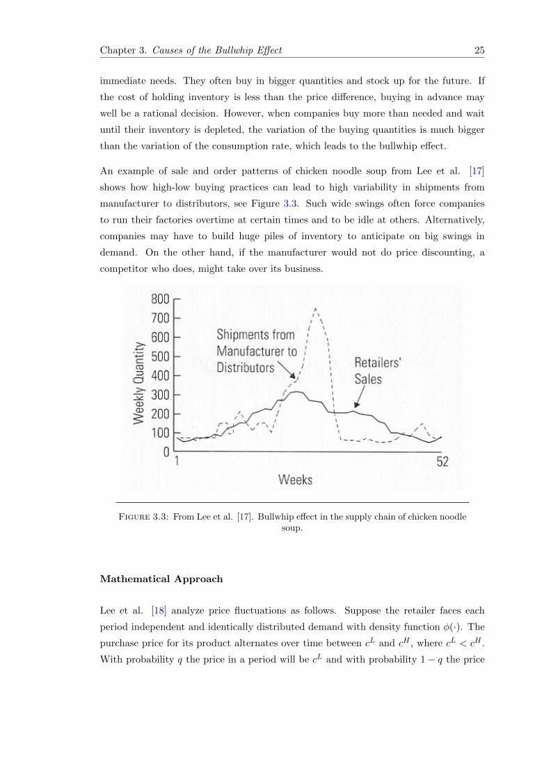
An example of sale and order patterns of chicken noodle soup from Lee et al. [17]

shows how high-low buying practices can lead to high variability in shipments from

manufacturer to distributors, see Figure 3.3. Such wide swings often force companies

to run their factories overtime at certain times and to be idle at others. Alternatively,

companies may have to build huge piles of inventory to anticipate on big swings in

demand. On the other hand, if the manufacturer would not do price discounting, a

competitor who does, might take over its business.

Figure 3.3: From Lee et al. [17]. Bullwhip effect in the supply chain of chicken noodlesoup.

Mathematical Approach

Lee et al. [18] analyze price fluctuations as follows. Suppose the retailer faces each

period independent and identically distributed demand with density function φ(·). The

purchase price for its product alternates over time between cL and cH , where cL < cH .

With probability q the price in a period will be cL and with probability 1− q the price

Chapter 3. Causes of the Bullwhip Effect 26

will be cH . In this situation, the retailer’s inventory problem can be formulated as

V i(x) = miny≥x

ci(y − x) + L(y) + β

∞∫0

[qV L(y − ξ) + (1− q)V H(y − ξ)]φ(ξ)dξ

,where

L(y) = p

∞∫y

(ξ − y)φ(ξ)dξ + h

y∫0

(y − ξ)φ(ξ)dξ. (3.21)

Here V i denotes the minimal expected discounted cost incurred throughout an infinite

horizon when the current price is ci, i ε L,H, L(·) is the sum of one-period inventory and

shortage costs at a given level of inventory. The unit shortage penalty cost is denoted

by p and the unit holding cost by h.

Without giving a proof of the result, Lee et al. [18] report the following optimal inventory

policy to problem (3.21).

At price cL, get as close as possible to the stock level SL. At price CH , bring the stock

level to SH , where SH < SL.

To show the causes of price fluctuations, we use the following example. Suppose that

the cost parameters are chosen such that SH = 30 and SL = 100. In period 0 the manu-

facturer’s price is low, and the retailer raises its inventory level to 100. For a number of

periods, the manufacturer’s price remains high, so the retailer does not order until the

inventory level hits below 30. The retailer orders up to 30 until the manufacturer drops

its price to cL. When this happens, the retailer orders up to 100 items until the price is

raised. Here we simulated this example with normally distributed demand with µ = 15

and σ = 5. The chance q on a low purchase price in a certain period is 10%. Figure 3.4

shows a typical result of a simulation run. The high peaks represent periods with a low

purchase price. The bullwhip effect can be clearly observed.

Figure 3.4: Bullwhip effect due to price fluctations and rational decision making.

Chapter 3. Causes of the Bullwhip Effect 27

3.2.4 Rationing and Shortage Gaming

When product demand exceeds supply, a manufacturer often rations its product to

customers. For example, the manufacturer then allocates its products in proportion to

the amount ordered by the different retailers. Retailers often anticipate on potential

shortages by exaggerating their real needs when they order. If demand drops later,

this will lead to small orders and cancellations. Lee et al. [17] call this overreaction

by customers, rationing and shortage gaming. This “gaming” results in misleading

information on the product’s real demand. To illustrate the effects of rationing gaming

on the variance amplification, consider a supply chain consisting of a manufacturer,

multiple wholesalers, and multiple retailers. If the manufacturer appears to be in short

of supply, wholesalers will play the rationing game to get a large share of the supply.

Assessing a possibility of the wholesaler not getting enough from the manufacturer,

retailers also play the rationing game. The effect is that demand and its variance are

amplified as one moves up the supply chain. In practice, there are many examples of

this rationing and shortage gaming. One example is the shortage of DRAM chips in

the 1980’s, from Lee et al. [18]. In the computer industry, orders for these chips grew

fast, not because a growth in customer demand, but because of anticipation. Customers

placed duplicate orders with multiple suppliers and bought from the first one that could

deliver, then cancelled all other duplicate orders.

Mathematical Approach

Lee et al. [18] developed a one-period model with multiple retailers to illustrate that

retailers rationally will issue an order which exceeds in quantity what the retailer would

order if the supply of the product is unlimited. A description is given below.

A manufacturer supplies a single product to N identical retailers indexed by n =

1, 2, . . . , N . Retailer n first observes its demand distribution Φ(·) and places an order zn

at time 0. Then, the manufacturer delivers the product at time 1. The manufacturer’s

output µ is a random variable, distributed according to F (·).In case the total amount of orders

∑Nn=1 zn exceeds the realized output µ, the manu-

facturer allocates the output to retailers in proportion to their orders. The total retail

orders are denoted by Q :=∑

j zj . If the realized capacity µ is smaller than Q, retailer

i will receive ziµ/Q due to the allocation.

Let Ci(z1, . . . , zi, . . . , zN ) denote the expected cost for retailer i when retailer i chooses

the order quantity zi for i = 1, 2, . . . , N . A Nash equilibrium is defined as the order

quantities (z∗1 , z∗2 , . . . , z

∗N ) chosen by retailers who each take the decisions of others as

given and choose zi to minimize the expected cost. That is, (z∗1 , z∗2 , . . . , z

∗N ) is a Nash

Chapter 3. Causes of the Bullwhip Effect 28

equilibrium if, for each i = 1, 2, . . . , N ,

z∗i = arg minzi

Ci(z1, . . . , zi−1, zi, zi+1 . . . , zN ). (3.22)

Thus, if the first-order condition approach is valid, the equilibrium must satisfy, for each

i,dCidzi

(z1, . . . , zi−1, zi, zi+1 . . . , zN )|zi=z∗i = 0. (3.23)

Since every retailer is symmetric, we focus on the symmetric Nash equilibrium where

z∗i = z∗ for each i = 1, 2, . . . , N . That is, z∗ satisfies

dCidzi

(z∗, . . . , z∗, zi, z∗ . . . , z∗)|zi=z∗i = 0. (3.24)

To derive the equilibrium, consider retailer i who takes the other retailers’ ordering

strategies z∗j (j 6= i) as given and chooses zi to minimize the expected cost

Ci =

Q∫µ=0

p ∞∫µzi/Q

(ξ − µzi

Q

)dΦ(ξ) + h

µzi/Q∫0

(µziQ− ξ)dΦ(ξ)

dF (µ)

+ (1− F (Q))

p ∞∫zi

(ξ − zi)dΦ(ξ) + h

zi∫0

(zi − ξ)dΦ(ξ)

, (3.25)

where Q =∑

j 6=i z∗j +zi and the unit shortage penalty cost is p. Note that the decision zi

must be taken before the capacity µ is realized. Hence, there are two possible scenarios

depending on the supply condition. One is when the supply µ falls short of the total

demand Q, and retailer i is allocated the amount ziµ/Q. The first term on the RHS of

(3.25) is the expected cost conditioned on the manufacturer’s output µ in the shortage

scenario. The other scenario is when the realized supply is sufficient to meet the total

demand. The second term on the RHS of (3.25) is the expected cost times the probability

of this scenario.

Its first order condition is given by

dCidzi

=

Q∫µ=0

[−p+ (p+ h)Φ

(µziQ

)]µ

(1

Q− ziQ2

)dF (µ)

+ [1− F (Q)][−p+ (p+ h)Φ(zi)] = 0, (3.26)

where we used Leibnitz’s rule and dQ/dzi = 1.

A pseudo-convex function is a function that behaves like a convex function with respect

to finding its local minima. If Ci is pseudo-convex, then the solution z0i to Equation

(3.26), is the optimal order quantity z∗i . To establish the pseudo-convexity of Ci, consider

Chapter 3. Causes of the Bullwhip Effect 29

Ci at z0i satisfying Equation (3.24). It must be that −p + (p + h)Φ(z0i ) ≥ 0, because

otherwise, we would have that −p + (p + h)Φ(µz0i /Q) ≤ 0 for all µ ≤ Q, resulting in

dCi/dzi < 0. Now, consider the second derivative of Ci w.r.t. z0i :

d2Cidz2i

= [−p+ (p+ h)Φ(z0i )]f(Q) + [1− F (Q)](p+ h)φ(z0i ) ≥ 0. (3.27)

This establishes the pseudo-convexity of Ci. It follows that the solution z0i to Equation

(3.26) is the optimal order quantity z∗i .

From (3.24) and (3.26), therefore, the symmetric equilibrium z∗ must satisfy

N ·z∗∫0

[−p+ (p+ h)Φ

( µN

)]µ

(1

N · z∗− 1

N2 · z∗

)dF (µ)

+[1− F (z∗ ·N)][−p+ (p+ h)Φ(z∗)] = 0. (3.28)

Theorem 3.3. In the above setting, z′ ≤ z∗, where z′ is the solution of the news-vendor

problem: −p + (p + h)Φ(z). The news-vendor problem is the problem with unlimited

supply. Further, if F (·) and Φ(·) are strictly increasing, the inequality strictly holds.

The theorem states that the optimal order quantity for the retailer in the rationing

game exceeds the order quantity in the traditional news-vendor problem. This implies

the bullwhip effect when the mean demand changes over time.

Chapter 4

Remedies to the Bullwhip Effect

Lee et al. [17][18] described four operational causes of the bullwhip effect. In Chapter

3 we gave an elaborate description of these causes. This chapter is concerned with

proposed remedies to counteract these four causes.

4.1 Remedies to Demand Signal Processing

Repetitive processing of demand data happens when supply chain members process

the demand signals from their immediate downstream neighbours. In this case, supply

chain members use the demand forecasts of their downstream neighbour to do their own

demand forecasts. In Paragraph 3.2.1 we showed how this could lead to the bullwhip

effect. In this paragraph, we present three commonly proposed remedies to the problem:

collaboration, replenishment smoothing, and operational efficiency.

4.1.1 Collaboration

Probably the most obvious remedy to the problem is collaboration between the supply

chain members. Canella et al. [4] define collaboration in a supply chain as “transforming

suboptimal solutions of individual links into a comprehensive solution through sharing

customer and operational information”. Several authors have shown how collaboration

could reduce the amplification of orders in the upstream direction (Chen et al. [6],

Disney et al. [9], Chatfield et al. [5]), reduce inventory holding costs (Shang et al. [21],

Kelepouris et al. [16]), and improve customer service levels (Hosada et al. [15]).

31

Chapter 4. Remedies to the Bullwhip Effect 32

A framework for different supply chain structures based on the degree of collaboration

was provided by Holweg et al. [14]. In their model they use the collaboration on inven-

tory replenishment and the collaboration on forecasting as dimensions, see Figure 4.1.

Figure 4.1: From Holweg et al. [14]. Supply chain collaboration framework.

The Traditional Supply Chain means that each level in the supply chain issues pro-

duction orders and replenishes stock without considering the situation at either

up- or downstream tiers of the supply chain.

In traditional supply chains the only information that is available to the upstream mem-

ber are the purchase orders issued by the downstream member. This is the setting of

Sterman’s beer game [22], described in Chapter 2. In Chapter 3 we saw that in this

setting the bullwhip effect will occur, even with rational decision making.

Information Exchange means that individual supply chain members still order inde-

pendently, yet exchange demand information and action plans in order to align

their forecasts for capacity and long-term planning.

Taking end customer sales into consideration at levels further upstream the supply chain

is a major improvement over simply relying on the orders sent by the downstream neigh-

bour. Delays in receiving the demand signals are removed, and unnecessary uncertainty

is eliminated.

Chapter 4. Remedies to the Bullwhip Effect 33

Vendor Managed Replenishment means that the task of generating the replenish-

ment order is given to the supplier, who then takes responsibility for maintaining

the retailer’s inventory, and subsequently, the retailer’s service levels.

Vendor Managed Replenishment (VMR), also often referred to as Vendor Managed In-

ventory (VMI) offers two sources of bullwhip reduction. One layer of decision making is

eliminated and the delays in information flow are reduced.

Synchronized Supply merges the replenishment decision with the production and

materials planning of the supplier. Here, the supplier takes charge of the customer’s

inventory replenishment on the operational level, and uses this visibility in planning

his own supply operations.

Collaboration on inventory replenishment and forecasting gives suppliers a better un-

derstanding and ability to cope with demand variability. This is an important feature

when trying to counter the bullwhip effect.

4.1.2 Replenishment smoothing

In practical situations, a commonly used periodic review policy is the (S,R) order policy.

At each review period R the inventory is reviewed and a quantity O is ordered to bring

the level of the available inventory to the order-up-to level S. The available inventory

consists of the inventory on hand plus the inventory on order but not yet arrived (Work

In Progress or Pipeline Inventory).

A smoothing replenishment rule is an (S,R) policy in which the entire gap between

the level S and the available inventory is not recovered in one review period. Instead,

for each review period R the quantity O is ordered to recover only a fraction of the

gap between the target on-hand inventory and the current level of on-hand inventory,

and a fraction of the gap between the target pipeline inventory and the current level of

pipeline inventory. The fractions to recover are regulated by decision parameters known

as proportional controllers. The proportional controller Ty modulates the recovery of

the on-hand inventory gap. The proportional controller Tw determines the recovery of

the work in progress inventory gap.

Smoothing replenishment is an effective remedy to demand signal processing, because

it limits the over-reaction/under-reaction to changes in demand. In the literature it

is shown that properly tuning the value of the proportional controllers can reduce the

bullwhip effect (Disney and Towill [10], Disney et al. [11]). However, smoothing replen-

ishment rules may have a negative impact on customer service (Dejonckheere et al. [7]).

This has only been shown in supply chains with no collaboration.

Chapter 4. Remedies to the Bullwhip Effect 34

4.1.3 Operational Efficiency

Many authors showed that long resupply lead times have a bad influence on the bullwhip

effect (Lee et al. [18], Chen et al. [6]). These lead times can be reduced by improving

the operational efficiency along the supply chain. An effective way to achieve this is

with just-in-time management (JIT). JIT is a method for inventory control that is part

of the lean manufacturing system. The philosophy of JIT is that the storage of unused

inventory is a waste of resources. To make the elimination of these inventory buffers

possible, the focus is on having the right material, at the right time, at the right place,

and in the exact amount. JIT controls production in a totally different way than MRP

does. MRP systems often run once a month and lead to large monthly orders. With

JIT, inventory spaces are reduced, which leads to frequent small orders and thus to short

lead times and smaller order batches. A disadvantage of JIT is that a small disruption,

for example a small change in demand or a broken machine, can immediately lead to

problems because the safety stocks are removed. On the other hand it makes quick

reactions possible because small disruptions are quickly observed.

4.2 Remedies to Order Batching

The second cause described by Lee et al. [17] is order batching. As shown by Lee et

al. [18], large order batches and low order frequencies contribute to the bullwhip effect,

and the effect is amplified if the order periods of different retailers are correlated.

In the previous section we described how the JIT method can counteract large order

batches and low order frequencies. However, small order batches and low order fre-

quencies are expensive. One reason is that the relative cost of placing an order and

replenishing it becomes higher if the order size decreases and/or if the order frequency

increases. A remedy is the use of Electronic Data Interchange (EDI), which is a method

for transferring data between different computer systems or computer networks. EDI

can reduce the cost of the paperwork in generating an order, which leads to more fre-

quent ordering by customers.

Another reason for large order batches is the otherwise high cost of transportation. Full

truckloads are often much more economical than less-than-full truckloads. A remedy

is the use of a third party logistics provider (3PL). A 3PL is a is firm that provides

multiple logistics services, under which transportation services that can be scaled and

customized to the needs of the customer. Third party logistics providers have many

customers and can combine orders of different customers, which makes it possible to

order less-than-full truckloads for an economical price.

Chapter 4. Remedies to the Bullwhip Effect 35

To reduce the amplification effect of correlated ordering, manufacturers could coordinate

their resupply with their customers. A manufacturer could for example spread the

regular delivery appointments with its customers as much as possible evenly over the

week.

4.3 Remedies to Price Fluctation

Companies sometimes buy items in advance of requirements in reaction to price fluc-

tuations. These price fluctuations often result from promotions like price discounts,

quantity discounts and coupons. Lee et al. [17] found that the costs of such practices

often outweigh the benefits and therefore it is better to stabilize prices. A common way

to do this is with a every day low price policy (EDLP). With EDLP companies offer no

discounts but promise a stable low price which saves customers the effort and expense

connected to price fluctuations. In practice, many companies use price discounts to

compete with other companies. Therefore, EDLP is for many companies not an option.

4.4 Remedies to Rationing and Shortage Gaming

When product demand exceeds supply, a manufacturer rations its product to customers.

In this situation the manufacturer often allocates its products in proportion to the

amount ordered by the different retailers. Retailers often anticipate on potential short-

ages by exaggerating their real needs when they order. A remedy proposed by Lee et al.

[17] is to allocate in proportion to past sales records, instead of allocating in proportion

to the amounts ordered. Customers then have no incentive to exaggerate their orders.

Another problem is that if demand drops later, companies can easily cancel their orders

due to the generous return policy of manufacturers. Without a penalty, retailers will

continue to exaggerate their needs and cancel their orders in case they ordered too much.

Lee et al. [17] therefore propose that manufacturers enforce more stringent cancellation

policies, so that retailers are more cautious with exaggerating their orders.

Chapter 5

Conclusion and Discussion

The bullwhip effect is an obstinate phenomenon that will always be present in supply

chains and cannot be completely eliminated. Since Forrester’s pioneering work [12] in

1961, much research has been done on the bullwhip effect. Many authors across a range

of academic disciplines showed the existence of the effect. Some authors ascribed solely

behavioural causes to the bullwhip effect. These causes are the misperception of time

legs, which lead to continued over- and underordering, and the use of suboptimal inven-

tory policies and forecasting techniques. Since two important papers of Lee et al. [17]

[18] in 1997, four operational causes are widely accepted as a complete explanation for

the bullwhip effect. These causes are demand signal processing, rationing and shortage

gaming, order batching and price fluctuation. Also, much research has been done on

the impact of different inventory policies, forecasting techniques, and other factors that

influence the process. These factors include the impact of forecast errors, lead times,

collaboration, seasonality, etcetera. The research on the bullwhip effect has led ‘among

others’ to a good explanation of the causes of the bullwhip effect and consequently to

many possible remedies.

Since the papers of Lee et al. [17] [18], there is little discussion about the causes of

the bullwhip effect. Unfortunately, countering the effect is in many practical situations

not that simple. Despite of all research that has been done on the subject, it remains

difficult to forecast the exact impact of certain changes or decisions in general. There

are many factors that have impact on the bullwhip effect and these factors have often

contradictory impacts in different circumstances. Moreover, the models that were used

to research the impacts of certain circumstances can not incorporate the complexity of

practical situations. For example, researchers often assume simple supply chains with

a single retailer, a single manufacturer, a single supplier etcetera. Supply chains in

practice, are often complex networks of many different companies.

37

Conclusion and Discussion 38

In practice, not one situation is the same and theoretical models are generally much

simplified. Therefore, the question raises what the value is of theoretical research on the

bullwhip effect. Exact numbers or formula’s are in my opinion only useful to compare

different scenarios in certain situations. Chen et al. [6] derived a lower bound on

the order rate variance ratio. In practical situations, this lower bound will often not

be correct, because it heavily depends on the demand model, the inventory policy,

forecasting technique and other assumptions. However, it gives an indication of the

impact of a change, for example a change in the lead time or an other parameter. My

opinion is that theoretical research on the bullwhip effect leads to more insight in the

process and makes managers more aware of the problem.

Bibliography

[1] Kurt Salmon Associates. Efficient consumer response: Enhancing consumer value

in the grocery industry. Kurt Salmon Associates, 1993.

[2] J. D. Blackburn. The quick-response movement in the apparel industry: a case study

in time-compressing supply chains. Time Based Competition: the Next Battleground

in American Manufacturing, 1991.

[3] G. P. Cachon and M. Fisher. Supply chain inventory management and the value of

shared information. Management Science, 46(8), 2000.

[4] S. Cannella and E. Ciancimino. On the bullwhip avoidance phase: supply chain

collaboration and order smoothing. International Journal of Production Economics,

48(22), 2010.

[5] D.C. Chatfield, J. G. Kim, T. P. Harrison, and J. C. Hayya. Impact of stochas-

tic lead time, information quality, and information sharing: a simulation study.

Production and Operations Management, 13(4), 2004.

[6] F. Chen, Z. Drezner, J. K. Ryan, and D. Simchi-Levi. Quantifying the bullwhip

effect in a simple supply chain: The impact of forecasting, lead times, and informa-

tion. Management Science, 46(3), 2000.

[7] J. Dejonckheere, S. M. Disney, M. R. Lambrecht, and D. R. Towill. Measuring and

avoiding the bullwhip effect: a control theoretic approach. European Journal of

Operational Research, 147(3), 2003.

[8] S. M. Disney and A. Potter. Bullwhip and batching: An exploration. International

Journal of Production Economics, 104(2), 2006.

[9] S. M. Disney and D. R. Towill. A discrete transfer function model to determine

the dynamic stability of a vendor managed inventory supply chain. International

Journal of Production Research, 40(1), 2002.

39

Bibliography 40

[10] S. M. Disney and D. R. Towill. On the bullwhip and inventory variance produced

by an ordering policy. Omega, the International Journal of Management Science,

31(3), 2003.

[11] S. M. Disney et al. Controlling bullwhip and inventory variability with the golden

smoothing rule. European Journal of Industrial Engineering, 1(3), 2007.

[12] J. W. Forrester. Industrial dynamics. MIT Press, Cambridge, MA, 1961.

[13] D. Heyman and M. Sobel. Stochastic models in Operations Research Vol. 1.

McGraw-Hill, New York, 1984.

[14] M. Holweg, S. Disney, J. Holmstrom, and J. Smaros. Supply chain collaboration:

making sense of the strategy continuum. European Management Journal, 23(2),

2005.

[15] T. Hosoda, M. M. Naim, S. M. Disney, and A. Potter. Is there a benefit to sharing

market sales information? linking theory and practice. Computers and Industrial

Engineering, 54(2), 2008.

[16] T. Kelepouris, P. Miliotis, and K. Pramatari. The impact of replenishment pa-

rameters and information sharing on the bullwhip effect: a computational study.

Computers and Operations Research, 35(11), 2004.

[17] H. L. Lee, V. Padmanabhan, and S. Whang. The bullwhip effect in supply chains.

Sloan Management Review, 38(3), 1997.

[18] H. L. Lee, V. Padmanabhan, and S. Whang. Information distortion in a supply

chain: The bullwhip effect. Management Science, 43(4), 1997.

[19] R. Metters. Quantifying the bullwhip effect in supply chains. Journal of Operations

Management, 15, 1997.

[20] J. K. Ryan. Analysis of Inventory models with limited demand information. PhD

thesis, Department of Industrial Engineering and Management Science, Northwest-

ern University, Evanstan 2, 1997.

[21] J.S. Shang, S. Li, and P. Tadikamalla. Operational design of a supply chain system

using the taguchi method, response surface methodology, simulation, and optimiza-

tion. International Journal of Production Research, 42(18), 2004.

[22] J. D. Sterman. Modeling managerial behavior: Misperceptions of feedback in a

dynamic decision making experiment. Management Science, 35(3), 1989.