The Budget and Tax Effects of a Federal Public Option After COVID-19Lanhee J. Chen, Ph.D., Tom Church, and Daniel L. Heil

October 20, 2020

1

The Budget and Tax Effects of a Federal Public Option After COVID-19Lanhee J. Chen, Ph.D., Tom Church, and Daniel L. Heil1

Abstract

A public option that follows historical trends would become the third-largest federal spending program and increase deficits by almost $800 billion over ten years. These increases are particularly problematic given the significant increases in deficits fueled by the relief packages enacted in the wake of the COVID-19 pandemic. We examine a variety of tax hike scenarios that could finance a public option and return federal debt projections to their pre-COVID-19 levels. Limiting the tax increases to high-earning households would produce marginal federal income tax rates of 60 percent in 2050, higher than any point in the last 40 years. Using broad-based taxes would require increasing all personal income tax rates by over 30 percent in 2050, raising taxes on middle-income families by over $2,000 a year. Alternatively, financing the public option with payroll taxes would require increasing the Hospital Insurance payroll tax by 180 percent in 2050, with taxes for typical families rising by over $3,900. In short, policymakers will likely need to choose between a number of significant tax hikes to help finance the high costs of a politically realistic public option.

1 Lanhee J. Chen, Ph.D. is the David and Diane Steffy Fellow in American Public Policy Studies at the Hoover Institution; Tom Church is a Policy Fellow at the Hoover Institution; Daniel L. Heil is a Policy Fellow at the Hoover Institution. The views expressed in this paper are those of the authors alone, and do not necessarily reflect the views of the Hoover Institution or Stanford University. This work was supported by the Partnership for America’s Health Care Future.

2

IntroductionPublic option proposals continue to garner significant attention and support. Proponents promise a federally run health insurance program that would offer lower premiums without increasing federal deficits. In Church, Heil, and Chen (2020), however, we explained why the assumptions underpinning these promises were politically unrealistic and inconsistent with past congressional behavior.2 Using more politically realistic assumptions, we now estimate the public option would increase federal deficits by nearly $800 billion in its first 10 years and would eventually become the third-largest government program.

The prospect of a costly new government program comes at an inopportune time. At the beginning of the 2020 fiscal year, the federal deficit was expected to exceed $1 trillion. The economic and legislative response to the COVID-19 pandemic then increased the deficit projection by an additional $2 trillion. The Congressional Budget Office (CBO) now projects the federal debt will reach 109 percent of GDP in 2030 and exceed 195 percent by 2050.3 This represents a substantial increase from CBO’s June 2019 forecast, which projected the 2049 federal debt would reach 144 percent of GDP.4

Without major spending reforms, avoiding this unprecedented increase in the federal debt will require significant tax increases. Policymakers must account for this prospect before enacting new spending programs. This is particularly true when considering expensive programs like a politically realistic public option, which would likely require further tax increases.

In this paper, we explore various tax increase options to finance a politically realistic public option. These range from a corporate tax increase to broad-based increases in payroll or personal income taxes. Attempting to limit these tax increases to corporations or high-income earners would require significantly higher rates that would produce large negative economic effects. Ultimately, we conclude that revenue demands of the public option would likely require broad-based tax increases.

Importantly, we assume any public option tax increase would be in addition to the tax increases needed to avoid the large projected increase in federal debt due to COVID-19-related relief and other recent federal spending increases. We estimate that, under the current baseline, all major sources of revenue (i.e., personal income taxes,

payroll taxes, and corporate income taxes) would need to rise by 10.4 percent beginning in 2026 to return projected debt to its pre-COVID-19 baseline (approximately 150 percent of GDP in 2050). Ensuring the public option does not add to federal deficits would require further tax increases. Personal income tax rates would need to rise by an additional 18 percent across-the-board, pushing the top federal marginal tax rate above 51 percent. Alternatively, the Medicare payroll tax would need to be set at 8.1 percent in 2050—a 179 percent increase in the current tax rate.

Ultimately, we conclude that revenue demands of the public option would likely require broad-based tax increases.

2 Church, Heil, & Chen (2020). 3 Congressional Budget Office (September 2020).4 Congressional Budget Office (June 2019).

3

Over the last two decades, public option proposals have been regularly debated. While their details vary, the proposals would establish a federally-run health insurance plan. The plan would charge actuarially fair premiums to enrollees that would fully cover the cost of the program.

Proponents predict premiums would be lower than competing private plans. Compared to private insurers, they argue, the federal government would have lower administrative costs and be able to negotiate reduced reimbursements rates for medical providers and hospitals. The lower premiums would have a positive effect on the federal budget. First, lower premiums would reduce the Affordable Care Act’s (ACA) marketplace exchange subsidies resulting in lower federal outlays and slight reductions in ACA-related tax expenditures. Second, reduced premiums for employer-sponsored insurance (ESI) plans would result in increased taxable income, leading to higher personal income tax and payroll tax revenue.

In Church, Heil, and Chen (2020), we examined the two major assumptions underpinning the optimistic public option budget scores: actuarially fair premiums and low reimbursement rates. We noted that existing federal health care programs, particularly Medicare, began with similar assumptions. The stringent assumptions, however, were quickly relaxed as Congress succumbed to political pressures. In the case of Medicare, Congress repeatedly

shielded recipients from scheduled premium increases and protected providers from cuts to reimbursement rates. Subsidies from taxpayers grew far beyond what was initially promised. If future congresses follow a similar path with respect to a public option, we found that the public option would quickly become an expensive new government program.

The politically realistic public option would initially begin with similar assumptions found in existing public option proposals. The plan would be available in the individual, small-group, and large-group health insurance markets.5 Reimbursements rates for hospitals and medical providers would be set near Medicare levels and premiums would be actuarially fair (subject to the ACA’s community rating requirements). Similar to the legislative history of Medicare, these initial assumptions would be quickly relaxed. Reimbursement rates would grow to private-insurer rates over five years and premium increases would be limited to the rate of inflation (CPI-U).

The implicit subsidy—the difference between the actuarially fair premiums and actual premiums charged—would be paid by the federal government. These implicit subsidies would increase federal outlays. Without additional revenue, deficits would increase as the implicit subsidy would grow far more quickly than cost savings from reductions in ESI tax expenditures and ACA subsidies.

I. An Overview of the Politically Realistic Public Option

If future congresses follow a similar path with respect to a public option, we found thatthe public option would quickly become an expensive new government program.

5 In our earlier paper, we included a scenario where the public option was limited to only individuals and small-group markets (firms with fewer than 50 employees). In this paper, we consider only a public option available in all markets. In addition, consistent with our earlier paper, we exclude those who are projected to be uninsured or enrolled in Medicaid. This assumption means the number of people purchasing health insurance (either from private insurers or the public option) matches CBO’s projections.

4

In June 2019, CBO projected the federal debt would rise to 144 percent of GDP in 2049.6 The debt, driven largely by spending increases in federal entitlement programs and rising interest expenses, would continue to grow beyond the 30-year budget window. Since June 2019, the outlook has become even more dire. CBO now projects debt to rise to 189 percent of GDP in 2049 and reach 195 percent in 2050.7

The large increase in projected debt is primarily a consequence of COVID-19 and the legislative response to the pandemic. The economic and budgetary effects of COVID-19 have been considerable. Some

effects stem from the economic impact of state shutdowns and widespread unemployment. Other effects come from federal legislation that was enacted to mitigate the pandemic’s financial impact.

The short-term economic effects are dramatic. CBO expects real GDP to remain below its 2019 level until 2022. The unemployment rate is projected to be 8.4 percent in 2021 and is expected to remain above 6 percent until 2025.8 The economic downturn means large reductions in revenue and will increase enrollment in low-income entitlement programs, ultimately increasing federal deficits. CBO expects these changes to be partially offset by low interest rates on the federal debt and reductions in projected inflation rates that will slow future outlay growth for major entitlement programs such as Social Security.

In addition to economic changes, the federal government has responded to the pandemic with large-scale federal spending programs and tax reductions. The first was the Coronavirus Preparedness and Response Supplemental Appropriations Act, signed on March 6, 2020. It increased outlays by $8 billion. The second was the Families First Coronavirus Response Act, signed into law on March 18, 2020. CBO estimated that it would increase deficits by $192 billion over ten years. The third was the Coronavirus Aid, Relief and Economic Security (CARES) Act, passed on March 27, 2020. It increased 10-year outlays by over $1.3 trillion and reduced revenue by $400 billion, adding $1.7 trillion to deficits. In addition, the CARES Act included tax deferments that further increased projected deficits in 2020 and 2021. Finally, the Paycheck Protection Program and Health Care Enhancement Act, passed on April 24, 2020, added an additional $483 billion in new spending.9

6 Congressional Budget Office (June 2019).7 Congressional Budget Office (September 2020).8 Congressional Budget Office (July 2020). 9 Congressional Budget Office (June 2020).

II. The Current Long-Term Federal Budget Baseline

Since June 2019, the outlook has become even more dire. CBO now projects debt to rise to 189 percent of GDP in 2049 and reach 195 percent in 2050.7

Ultimately, our earlier estimate found that the politically realistic public option would increase federal deficits by over $700 billion in its first 10 years, and the plan would eventually become the third-largest government program. Since our initial projections, large economic and budget changes have altered the fiscal landscape. Below we explore how these changes affect the larger budget and the viability of a public option.

5

While there is considerable debate regarding the economic effects of higher debt, CBO expects the increased borrowing to have significant effects on the economy. Growing deficits reduce domestic private investment and increase debt payments to foreign investors. The result will be lower gross national product (GNP) than if lower debt levels were sustained. In its 2019 Long-Term Budget Outlook, CBO noted that reducing 2049 debt levels to 42 percent of GDP would raise GNP per capita by $5,500 in 2019 dollars.11 The recent increases in federal borrowing increase the likely harmful economic effects of additional deficit-financed spending.

These new projections cast further doubt on the prudence of enacting a public option that could further increase federal borrowing. In the section below, we estimate the long-run fiscal effects of a politically realistic public option that is financed through deficit spending.

75%

100%

125%

150%

175%

200%

2019 2024 2029 2034 2039 2044 2049

Figure 1. Long-Term Federal Debt Projections: June 2019 vs September 2020 (Percent of GDP)

June 2019 September 2020

Beyond COVID-19-related changes to the budget, in August 2019 Congress passed the Bipartisan Budget Act of 2019. The Act raised discretionary spending caps by nearly $300 billion for the 2020 and 2021 fiscal years. Due to CBO scoring methodology, however, the two-year changes resulted in a permanent increase in the discretionary spending baseline, further increasing long-term debt projections.10

The changes in the federal budget since June 2019 have exacerbated an already dire budget picture. Figure 1 shows the 2019 and 2020 CBO long-term debt projections. The federal debt is now expected to surpass 100 percent of GDP in FY2021—more than a decade sooner than previously projected—and will reach 195 percent by 2050. Deficits, which CBO previously projected at nearly 9 percent of GDP in 2049, are now expected to reach 12.6 percent that year.

10 For details see Committee for a Responsible Federal Budget (July 25, 2019).11 CBO uses gross national product rather than GDP “because it is a more complete measure of the income available to U.S. residents.” Congressional Budget Office (June 2019).

6

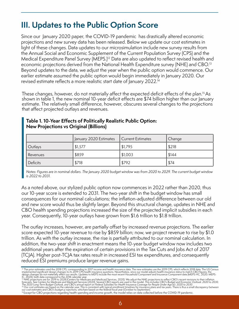
As a noted above, our stylized public option now commences in 2022 rather than 2020, thus our 10-year score is extended to 2031. The two-year shift in the budget window has small consequences for our nominal calculations; the inflation-adjusted difference between our old and new score would thus be slightly larger. Beyond this structural change, updates in NHE and CBO health spending projections increased the size of the projected implicit subsidies in each year. Consequently, 10-year outlays have grown from $1.6 trillion to $1.8 trillion.

The outlay increases, however, are partially offset by increased revenue projections. The earlier score expected 10-year revenue to rise by $859 billion; now, we project revenue to rise by $1.0 trillion. As with the outlay increase, the rise is partially attributed to our nominal calculation. In addition, the two-year shift in enactment means the 10-year budget window now includes two additional years after the expiration of certain provisions in the Tax Cuts and Jobs Act of 2017 (TCJA). Higher post-TCJA tax rates result in increased ESI tax expenditures, and consequently reduced ESI premiums produce larger revenue gains.

Table 1. 10-Year Effects of Politically Realistic Public Option: New Projections vs Original (Billions)

Notes: Figures are in nominal dollars. The January 2020 budget window was from 2020 to 2029. The current budget window is 2022 to 2031.

January 2020 Estimates Current Estimates Change

Outlays $1,577 $1,795 $218

Revenues $859 $1,003 $144

Deficits $718 $792 $74

These changes, however, do not materially affect the expected deficit effects of the plan.15 As shown in table 1, the new nominal 10-year deficit effects are $74 billion higher than our January estimate. The relatively small difference, however, obscures several changes to the projections that affect projected outlays and revenues.

III. Updates to the Public Option ScoreSince our January 2020 paper, the COVID-19 pandemic has drastically altered economic projections and new survey data has been released. Below we update our cost estimates in light of these changes. Data updates to our microsimulation include new survey results from the Annual Social and Economic Supplement of the Current Population Survey (CPS) and the Medical Expenditure Panel Survey (MEPS.)12 Data are also updated to reflect revised health and economic projections derived from the National Health Expenditure survey (NHE) and CBO.13

Beyond updates to the data, we adjust the year when the public option would commence. Our earlier estimate assumed the public option would begin immediately in January 2020. Our revised estimate reflects a more realistic start date of January 2022.14

12 The prior estimates used the 2018 CPS, corresponding to 2017 income and health insurance data. The new estimates use the 2019 CPS, which reflects 2018 data. The US Census implemented significant design changes to its 2019 CPS health insurance questions. Nevertheless, since our model adjusts health insurance status to match CBO figures, the design changes do not materially affect our results. Updates to MEPS include the most recent Household Component and Insurance Component data (MEPS-HC, 2020; MEPS-IC, 2020); both data correspond to the 2018 calendar year.13 NHE projections are for 2019 to 2028 (Centers for Medicare and Medicaid Services, 2020). We adjust the NHE projections to reflect CBO’s recent revisions to their inflation forecasts. See Centers for Medicare and Medicaid Services (2020). Several CBO reports are used in the model. This includes CBO’s Budget and Economic Outlook: 2020 to 2030, The 2020 Long-Term Budget Outlook, and CBO’s annual report on Federal Subsidies for Health Insurance Coverage for People Under Age 65: 2020 to 2030.14 Our cost estimates are based on the calendar year. This is consistent with typical enrollment timelines for insurance plans and tax years. There is thus a small discrepancy between our cost estimates and CBO’s budget p rojections, whichare based on the federal fiscal year (October to September).15 Except for CBO projections regarding health spending and income growth, the model relies on data collected before the COVID-19 pandemic.

7

-1.0%0.0%1.0%

2.0%3.0%4.0%

2022 2027 2032 2037 2042 2047

Figure 2. Long-Term Effects of the Public Option(Percent of GDP)

Revenue Primary Outlays Primary Deficit

As discussed above, the politically realistic public option assumes that the federal government fails to charge actuarially fair premiums that would cover its costs. The magnitude of the implic-it subsidy is determined by the difference between health care cost growth, which determines the cost per enrollee, and price inflation (using the CPI-U), which determines actual premiums charged to enrollees and the ensuing total public option enrollment.

While long-term price inflation is only expected to grow at 2.2 percent per year, annual health expenditures are expected to grow at over 4 percent. In 2031, the mean subsidy per enrollee for a 40-year-old would be $2,820 (2020 dollars)—32.4 percent below the actuarially fair pre-mium.16 In 2050, the subsidy per enrollee for a 40-year-old grows to $6,970, and the federal government would pay for over half of the costs of the public option.

The large implicit subsidy would lead to increased take-up. By 2031, enrollment would exceed 139 million and grow to over 174 million by 2050. The result would be a costly government pro-gram that increases federal non-interest outlays by more than $1 trillion in 2050 (in 2020 dollars). The costly public option would worsen an already bleak budget picture.

Figure 2 presents the 30-year budget changes from the public option. The figure excludes any additional interest expense from rising deficits. The public option would increase primary outlays by 3.3 percent of GDP in 2050. At that point, the public option would be the third-largest government program behind only Medicare and Social Security and account for over one-eighth of non-interest outlays. This would be partially offset by an increase in revenue, but the 2050 primary deficit would still rise by 2.1 percent of GDP.

Borrowing costs related to the public option would further increase deficits. By 2050, interest outlays would total 9.4 percent of GDP, making it the single largest spending component of the budget. By 2050, a debt-financed public option would increase deficits by 3.1 percent of GDP. As shown in figure 3, a debt-financed public option would increase 2050 deficits by 3.4 percent of GDP.16 Since premiums are age-adjusted, the dollar amount of the implicit subsidy depends on the age of the enrollee; the percent below the actuarially fair premium is constant across ages.

8

0%3%6%9%

12%15%18%

2019 2024 2029 2034 2039 2044 2049

Figure 3. Deficit Projections With and Without a Politically Realistic Public Option (Percent of GDP)

June 2019 Current Baseline With Public Option

Notably, these projections assume historically low interest rates. This exposes the federal bud-get to considerable risk if interest rates rise unexpectedly. With debt levels above 100 percent of GDP, a 1 percentage point increase in interest rates will increase interest outlays by more than 1 percent of GDP. Thus, even small changes in interest rates will substantially alter the budget outlook.

The debt-financed public option would push federal debt as a percent of GDP to 226 percent in 2050. Figure 4 shows the debt path with and without the politically realistic public option. With the public option, debt would surpass 144 percent of GDP in 2040—9 years ahead of CBO’s 2019 forecast.

75%100%125%150%175%

200%225%

2019 2024 2029 2034 2039 2044 2049

Figure 4. Debt Projections With and Without a Politically Realistic Public Option (Percent of GDP)

June 2019 Current Baseline With Public Option

9

This fiscal scenario is not sustainable. Annual deficits amounting to more than one-tenth the size of the economy represent unchartered fiscal territory for the U.S. They threaten to slow the economy and mean that small increases in interest rates would have massive implications for the federal budget.

Absent substantive spending reforms, avoiding the projected increases in the federal debt will require permanent tax increases. These tax increases would be necessary to finance the large projected increase in future outlays, as well as any additional spending from new policies such as a politically realistic public option. Below, we estimate the magnitude of the tax increases needed to return debt projections to CBO’s 2019 forecast and finance a politically realistic public option, under a variety of scenarios.

We model 30-year revenue estimates for several federal tax categories.17 We then estimate the annual percent change in revenue needed to reach our 2050 debt target or finance the annual costs of the politically realistic public option. Depending on the particular simulation, we change one or more of the following taxes: personal income taxes, the Social Security payroll tax (OASDI), the Hospital Insurance payroll tax (HI), the ACA’s additional Medicare tax and the Net Investment Income Tax (NIIT), and the corporate income tax.18 We do not consider base-broadening options such as limiting the ESI tax exclusion or eliminating other deductions. We also do not consider new tax vehicles like a Value-Added Tax, a carbon tax, or various excise tax options like those included in the ACA.

Unless otherwise noted, the tax estimates are static calculations that assume individuals and businesses do not change their behavior in response to tax rate changes. This is particularly important when we consider large changes in top rates, corporate income taxes, or changes in the taxation of investment income. Such large tax increases could lead to significant changes in behavior that could result in far less revenue than our static estimates predict. As such, our tax rate changes likely represent the lower bound of the increases needed to raise the required revenue.

We first estimate the size of the across-the-board tax increase needed to return the budget baseline to its 2019 trajectory. We then explore tax increase options to finance the public option. These tax increases would be in addition to our base tax increase.

We examine five options: 1. Raising the corporate tax rate 2. Increasing the ACA’s additional Medicare tax and the NIIT 3. Raising the top three personal income tax rates 4. Raising all personal income tax rates 5. Increasing the HI payroll tax

IV. Tax Policy Options to Finance a Costly Public Option at the Pre-COVID-19 Baseline

17 We use CBO’s Long-Term Budget Outlook and our microsimulation for these estimates. The calculations are summarized in the appendix. 18 We assume any payroll tax increase is levied on the employee only. This simplifies the calculations since an employer-side payroll tax increase would reduce wages, decreasing personal income tax revenue.

10

Returning to the 2019 BaselineBefore considering tax increases needed to finance a politically realistic public option, we first consider the rate increases necessary to keep federal debt below 150 percent of GDP through 2050. This target is consistent with CBO’s 2019 debt projection, which forecasted debt would reach 144 percent of GDP in 2049. We refer to this tax increase as the “base tax increase.”

Importantly, our debt target does not reflect an estimate of an optimal debt level. Even with our tax increases, the debt-to-GDP ratio would continue to rise far beyond our specified target after 2050. Thus, policymakers should view the base tax increase presented here as a lower bound of the rates needed to produce a sustainable fiscal outlook without substantial spending reforms.

While there are countless tax configurations possible to achieve this debt reduction, we assume an across-the-board tax increase on all major categories: corporate, personal income, and payroll taxes. This includes both the additional Medicare tax and the NIIT. We implement the tax increase in 2026 when most of the personal income tax provisions of the TCJA expire.

Starting from the post-TCJA rates, an across-the-board tax increase of 10.4 percent would be required to keep long-term federal debt below 150 percent of GDP. New marginal personal income tax rates would start at 11 percent and top out at 43.7 percent. Combined payroll taxes would rise to 16.9 percent, and the corporate tax rate would increase to 23.2 percent. Figure 5 shows how total federal revenue as a percent of GDP would be affected by our base tax increase.

Figure 6 compares the debt projections of the base tax increase with CBO’s 2020 and 2019 debt projections. The debt-to-GDP ratio would decline between 2026 and 2035, but then would begin to rise and closely follow CBO’s 2019 debt projections.

15%

17%

19%

21%

2020 2025 2030 2035 2040 2045 2050

Figure 5. Total Revenue: Current Baseline With and Without Across-the-Board Tax Increase (Percent of GDP)

Current Baseline With Base Tax Increases

11

19 The base tax increase slightly changes the public option score presented in section III. Revenue savings from reduced ESI premiums are slightly larger, with higher personal income and payroll tax rates. We account for these changes in our subsequent tax calculations. 20 Joint Committee on Taxation (2013).

We now turn to tax options to finance a politically realistic public option. Importantly, all of the tax options considered below are in addition to our base tax increase.19

75%100%125%150%175%

200%225%

2020 2025 2030 2035 2040 2045 2050

Figure 6. Debt Projections: 2019 Baseline, Current Baseline, & Baseline With Across-the-Board Tax Increase (Percent of GDP)

June 2019 Current Baseline With Base Tax Increases

The first option raises corporate taxes by the amount required each year to pay for the public option while keeping long-term debt at 150 percent of GDP. This option may be looked on favorably because the legal incidence of the taxation does not fall on workers. It would only be levied on profitable firms. Nevertheless, economists expect a portion of the tax to be paid by workers in the form of lower wages and consumers in the form of higher prices. CBO, for example, has previously assumed that workers bear 25 percent of the corporate tax.20

The TCJA permanently lowered the corporate tax rate from 35 percent to 21 percent. Adding the across-the-board base tax increase would raise the rate to 23.2 percent starting in 2026. With the base tax increase, revenue from the corporate income tax would total 1.4 percent of GDP in 2050.

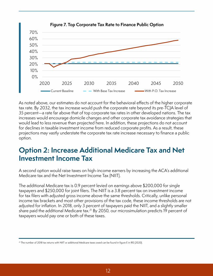
As the public option would expand the 2050 primary deficit by 2.1 percent of GDP, the corporate tax rate would have to rise from its new baseline of 23.2 percent to 58.0 percent by 2050. Notably, this includes three years where short-term revenues outpace outlays, leading to temporarily lower corporate tax rates. Overall, corporate tax revenue would rise from 1.4 percent of GDP (with the base tax increase) to 3.5 percent of GDP in 2050.

Option 1: Increase Corporate Taxes

12

As noted above, our estimates do not account for the behavioral effects of the higher corporate tax rate. By 2032, the tax increase would push the corporate rate beyond its pre-TCJA level of 35 percent—a rate far above that of top corporate tax rates in other developed nations. The tax increases would encourage domicile changes and other corporate tax avoidance strategies that would lead to less revenue than projected here. In addition, these projections do not account for declines in taxable investment income from reduced corporate profits. As a result, these projections may vastly understate the corporate tax rate increase necessary to finance a public option.

0%10%

20%30%40%50%60%70%

2020 2025 2030 2035 2040 2045 2050

Figure 7. Top Corporate Tax Rate to Finance Public Option

Current Baseline With Base Tax Increase With P.O. Tax Increase

Option 2: Increase Additional Medicare Tax and Net Investment Income TaxA second option would raise taxes on high-income earners by increasing the ACA’s additional Medicare tax and the Net Investment Income Tax (NIIT).

The additional Medicare tax is 0.9 percent levied on earnings above $200,000 for single taxpayers and $250,000 for joint filers. The NIIT is a 3.8 percent tax on investment income for tax filers with adjusted gross income above the same thresholds. Critically, unlike personal income tax brackets and most other provisions of the tax code, these income thresholds are not adjusted for inflation. In 2018, only 3 percent of taxpayers paid the NIIT, and a slightly smaller share paid the additional Medicare tax.21 By 2050, our microsimulation predicts 19 percent of taxpayers would pay one or both of these taxes.

21 The number of 2018 tax returns with NIIT or additional Medicare taxes owed can be found in figure E in IRS (2020).

13

22 Tax Foundation (2013).

Both taxes have narrow bases from which to raise revenue. Consequently, paying for the public option by raising both the additional Medicare tax and the NIIT would require significant rate increases. By 2050, each rate would have to rise by 472 percent. The additional Medicare tax would be set at 5.2 percent, and the NIIT would be set at 24.0 percent. The combined tax increases would significantly change marginal tax rates for high earners. The new NIIT rate would nearly double the current long-term capital gains rate for all affected taxpayers. In this scenario, the top marginal long-term capital gains tax rate would be 44 percent.

Such high tax rates would alter capital gains realizations, increase tax avoidance strategies, and reduce incentives to invest. Actual revenue collected would thus fall far short of our static estimates. As such, it seems unlikely that policymakers could expect to finance the public option through these tax measures alone.

Option 3: Increase Income Tax Rates of the Top Three BracketsOur third option raises personal income tax rates on top wage earners. Here, we consider how much personal income tax rates would have to rise for earners in the top three income tax brackets.

By 2050, financing the public option would require the top three rates to each rise by 37.4 percent. That would be in addition to the 10.4 percent base tax increase. As shown in figure 8, increasing only those three brackets in order to pay for the public option would raise the top tax rate to 60.1 percent. Taxpayers in the three highest brackets would be subject to federal marginal tax rates not seen since 1981.22

33.0% 35.0% 39.6%36.4% 38.6% 43.7%50.1% 53.1%

60.1%

0%

20%

40%

60%

80%

Third Highest Bracket Second Highest Bracket Top Bracket

Figure 8. 2050 Top Personal Income Tax Rates With and Without the Public Option Tax Increase

Current Baseline With Base Tax Increase With P.O. Tax Increase

14

23 See table 3.3 in IRS (2020).

Who would face these higher tax rates? In 2017 (the final year prior to the TCJA’s temporary bracket changes), the third-highest tax bracket began at $191,650 for single taxpayers and $233,350 for joint filers. In that same year, there were 7.7 million returns with taxable income over $200,000.23

Again, this analysis uses static projections that underestimate the true tax rate necessary to raise additional revenue. When including state income taxes, top marginal income tax rates could exceed 70 percent for some taxpayers. The effects on labor and investment decisions would be significant.

Option 4: Increase Personal Income Taxes Across the Board Raising the corporate income tax or taxes that fall only on high-income tax earners may be politically appealing. Nevertheless, it is unlikely that any of the tax increases presented above would be economically viable. The revenue demands of a politically realistic public option would likely require taxes be raised on a much broader tax base. Thus, option 4 raises all personal income tax rates by a proportional amount.

Even with a broader base, however, 2050 personal income tax rates would still need to rise by 30.3 percent to reach our debt target and fully finance the public option. That includes a 10.4 percent base tax increase and an additional 18.0 percent increase for the public option. Middle-income personal income tax rates would reach 32.6 percent. The top personal income rate would rise to 51.6 percent—higher than any time since 1981. Figure 9 shows the new tax rates for each existing bracket. The figures include the base tax increase.

10.0%15.0%

25.0% 28.0%33.0% 35.0%

39.6%

13.0%19.5%

32.6%36.5%

43.0% 45.6%51.6%

0%

20%

40%

60%

Bottom Rate Second Third Fourth Fifth Sixth Top Rate

Figure 9. 2050 Personal Income Tax Rates With and Without an Across-the-Board Public Option Personal Income Tax Increase

Current Baseline With P.O. and Base Tax Increase

15

Table 2 shows the estimated inflation-adjusted median tax increases by income quintile in 2050. The public option would raise taxes for American households in the middle quintile by $1,018 that year (2020 dollars). This would be in addition to the $1,362 they would pay from the base tax increase.

The across-the-board personal income tax increases are indeed more moderate than earlier options, but they would still have negative effects on the economy and the labor force. A 30 percent increase in personal income taxes would likely discourage work, reducing the labor supply and ultimately taxable income. And as a static estimate, the actual income tax rate increase needed to finance the public option would be even larger. Finally, these tax increases will likely cause political headaches because of their broad-based nature, with higher taxes broadly distributed across American households of all incomes, even those with modest earnings.

Option 5: Increase the Medicare Hospital Insurance Payroll Tax RateRaising personal income tax rates maintains the progressivity of the tax code, but as shown above, the demands of the public option would ultimately push top marginal tax rates above 50 percent. State income taxes would mean some taxpayers would face marginal rates over 60 percent. Such high tax rates would create particularly large economic distortions. Alternatively, our final option avoids high marginal tax rates by financing public option costs through an increase in the Medicare Hospital Insurance (HI) payroll tax.24

24 This expanded revenue would not be earmarked to pay for Medicare operations or to fund the Hospital Insurance Trust Fund. It would directly subsidize the public option in order to keep it deficit neutral.

Table 2. 2050 Median Taxes Paid by Quintile After Across-the-Board Personal Income Tax Increases (2020 $)

First Second Middle Fourth Highest

Current Balance $0 $5,747 $13,083 $26,264 $68,573

Base Tax Increase $0 $598 $1,362 $2,734 $7,138

Public Option Tax Increase

$0 $335 $1,018 $2,569 $7,977

Total Tax Increase $0 $933 $2,380 $5,303 $15,116

16

Currently, the HI tax is a 2.9 percent tax rate levied on all wages and salaries. Officially, the tax is split evenly between employers and employees, but CBO and most economists assume workers bear most of the employer-share of the tax in the form of lower wages.25 To finance the public option, the HI tax would need to rise by 153 percent by 2050. This would be in addition to the 10.4 percent base tax increase. Figure 10 shows that the total HI tax would have to rise to 8.1 percent by 2050 to finance the public option and meet our debt target.

Unlike the options presented above, this tax hike would reduce the overall progressivity of the tax code since the HI rate applies to all earnings equally. As such, taxes on lower- and middle-income workers would rise by more than in the scenario where federal income tax rates are increased across-the-board. We estimate that the public option and the base tax increase combined would increase taxes on middle-income households by $3,909 in 2050 (2020 dollars). Table 3 provides median tax increases by quintile.

25 See page 38 in Congressional Budget Office (2018).

0.0%2.0%4.0%6.0%8.0%

10.0%

2020 2025 2030 2035 2040 2045 2050

Figure 10. Medicare Payroll Tax Rate With and Without Public Option Tax Increases

Current HI Tax With Base Tax Increase With P.O. Tax Increase

Table 3. 2050 Median Taxes Paid by Quintile After Payroll Tax Increase (2020 $)

First Second Middle Fourth Highest

Current Balance $0 $5,747 $13,083 $26,264 $68,573

Base Tax Increase $0 $598 $1,362 $2,734 $7,138

Public Option Tax Increase

$0 $1,433 $2,547 $4,342 $8,968

Total Tax Increase $0 $2,031 $3,909 $7,076 $16,106

17

Our microsimulation predicts that the 153 percent increase in the HI tax would raise marginal tax rates from 35.4 percent (including the base tax increase) to 40.3 percent. Mean after-tax wages would accordingly fall by about 7.5 percent. This large tax increase would have broad effects on labor supply and ultimately reduce taxable income. We estimate that the mean labor supply would fall by at least 1.5 percent in 2050 in response to this higher tax rate.26 The decline in labor supply would ultimately mean a smaller economy and, therefore, directly reduce our tax revenue projections.

Accounting for those dynamic changes would require 2050 payroll taxes to rise by an additional 0.7 percentage points, from 8.1 percent to 8.8 percent. This tax increase would be paid by every wage-earner in the country, pushing combined OASDI and HI payroll taxes from the existing 15.3 percent tax to 21.2 percent. Middle-income families in the third-lowest income tax bracket would have federal marginal rates above 40 percent.

26 We discuss these calculations in the appendix.

18

One year of vastly increased federal spending due to the novel coronavirus effectively fast-forwarded the federal debt by over ten years. Last year, public debt was expected to exceed the size of the economy in 2034. It will now occur in FY2021.

An economic recovery is required in the short-term, but long-term deficits need to be addressed. An across-the-board base tax increase of at least 10.4 percent on all corporate, personal income, and payroll tax rates would return the long-term debt trend to what it was pre-COVID-19. Fully accounting for the dynamic effects of the taxes would likely raise the required tax increase substantially. Even under the best-case scenario, the tax increase would still mean federal debt as a share of the economy would continue to increase in the long run.

Adding any new spending program on top of an already debt-heavy future should be done with extreme caution. The public option is a program that, at first glance, appears to expand health insurance coverage in a deficit-neutral way. But as we have demonstrated, its likely short- and long-term futures are that of government subsidies and increased federal borrowing.

Paying for public option subsidies in the form of relatively narrow tax bases like the corporate income tax, the ACA’s additional Medicare tax and Net Investment Income Tax, or confining personal income tax increases to top income brackets would lead to prohibitively high marginal tax increases. These rates would likely lead to significant economic consequences and are unlikely to raise sufficient revenue to cover the costs of the public option. The trade-off to limiting this economic harm is that more efficient, broad-based tax increases would raise tax burdens for middle- and low-income taxpayers.

Making long-term budget projections is inherently limited by the assumptions made. This 30-year projection uses CBO estimates that assume relatively constant trends over time. But what happens in the next crisis, when Congress decides it is necessary to deviate from existing eligibility requirements or subsidy levels? In 2020, the federal government demonstrated its willingness to break from existing trends in order to provide immediate assistance. Future research that considers more abrupt changes to reimbursement rates or premium-setting rules is needed to shed further light on the fiscal risks of a public option.

V. Conclusion

19

Sources CitedCenters for Medicare and Medicaid Services, (2020). National Health Expenditure Survey (NHE). Available at: https://www.cms.gov/Research-Statistics-Data-and-Systems/Statistics-Trends-and-Reports/NationalHealthExpendData/NationalHealthAccountsProjected

Church, Tom, Daniel L Heil, and Lanhee J. Chen (January 2020). The Fiscal Effects of the Public Option. Available at: https://americashealthcarefuture.org/wp-content/uploads/2020/01/Final-The-Fiscal-Effects-Of-The-Public-Option-1.24.20.pdf

Church, Tom and Heil, Daniel (2019). “A Technical Overview of the Collection of Health Expenditures and Insurance (CHEI) Datasets.” Hoover Institution Economic Working Paper 19115. Available at: https://www.hoover.org/research/technical-overview-collection-health-expenditures-and-insurance-chei-data

Committee for a Responsible Federal Budget (July 25, 2019). Addressing Common Claims About the Budget Deal. Available at: https://www.crfb.org/blogs/addressing-common-claims-about-budget-deal

Congressional Budget Office, (2012). How the Supply of Labor Responds to Changes in Fiscal Policy. https://www.cbo.gov/sites/default/files/cbofiles/attachments/10-25-2012-Labor_Supply_and_Fiscal_Policy.pdf

Congressional Budget Office, (2018). The Distribution of Household Income, 2014. Available at: https://www.cbo.gov/publication/53597

Congressional Budget Office (June 2019). The 2019 Long-Term Budget Outlook. Available at: https://www.cbo.gov/publication/55331

Congressional Budget Office (June 2020). The Budgetary Effects of Laws Enacted in Response to the 2020 Coronavirus Pandemic, March and April 2020. Available at: https://www.cbo.gov/publication/56403

Congressional Budget Office (July 2020). 10-Year Economic Projections. Available at: https://www.cbo.gov/data/budget-economic-data#4

Congressional Budget Office (September 2020). The 2020 Long-Term Budget Outlook. Available at: https://www.cbo.gov/publication/56516

Internal Revenue Service (IRS) (2020). “Individual Income Tax Returns Complete Report,” Statistics of Income. Available at: https://www.irs.gov/pub/irs-pdf/p1304.pdf

Joint Committee on Taxation, (2013). Modeling the Distribution of Taxes on Business Income. Available at https://www.jct.gov/publications.html?func=startdown&id=4528

Medical Expenditure Panel Survey Household Component (MEPS-HC) (2020). Agency for Healthcare Research and Quality. Available at: https://meps.ahrq.gov/mepsweb/survey_comp/household.jsp

Medical Expenditure Panel Survey Insurance Component (MEPS-IC) (2020). Agency for HealthcareResearch and Quality. Available at: https://meps.ahrq.gov/survey_comp/Insurance.jsp

Tax Foundation (2013). U.S. Federal Individual Income Tax Rates History, 1862-2013 (Nominal and Inflation-Adjusted Brackets). Available at:https://taxfoundation.org/us-federal-individual-income-tax-rates-history-1913-2013-nominal-and-inflation-adjusted-brackets/

20

In estimating the necessary rate increases, we rely primarily on aggregate tax revenue estimates from CBO’s Long-Term Budget Outlook. This ensures our revenue changes are consistent with CBO’s budget projections. CBO does not include revenue estimates for specific payroll taxes, the NIIT, the additional Medicare tax, or tax revenue generated at each personal income tax bracket.

Adjustments to the Aggregate DataWe supplement the aggregate CBO estimates with data from our microsimulation’s tax model.27 The microsimulation data is also used to estimate changes in future tax burdens by income quintile and changes in marginal tax rates used in our dynamic estimates.

Our microsimulation tax model relies on data from the Annual Social and Economic Supplement of the Current Population Survey (CPS). Importantly, the CPS suffers from several data limitations that affect our revenue estimates. First, the survey does not differentiate between long-term and short-term capital gains, qualified and unqualified dividends, or taxable and non-taxable interest income. We thus treat all income sources as ordinary income. In addition, the CPS underestimates capital gains income and income in the top tax bracket, which underestimates the additional Medicare tax, the NIIT, and top personal income tax rates.

The additional Medicare tax levies a 0.9 percent tax on all earnings above $200,000 for single filers and $250,000 for married filers. The NIIT adds a 3.8 percent tax on investment income for tax filers with incomes above those thresholds. Relying on CPS estimates of incomes above these levels would result in an underestimate of the expected revenue from these taxes. Consequently, we use revenue estimates derived from the Open Source Policy Center’s Tax Brain to estimate aggregate 10-year revenue projections for these taxes.28 After 2029, we assume revenue from these sources grows at the same rate as predicted in our microsimulation’s tax model.

For personal income taxes, we divide aggregate revenue by the amount raised in each tax bracket and from the NIIT. We use data from the IRS Statistics of Income to determine the initial share of tax revenue generated at each tax bracket.29 We then grow the shares at rates consistent with the microsimulation estimates. The estimated shares are then multiplied by CBO’s aggregate personal income tax revenue (less revenue attributed to the NIIT) to determine the amount of revenue generated in each bracket for each year.

Likewise, since CBO’s 30-year projections do not disaggregate payroll taxes by type, we use the microsimulation estimates to determine the amount of revenue for OASDI and HI. We then adjust the estimates to ensure the sum of OASDI, HI, the additional Medicare tax, and other payroll taxes, is equal to CBO’s aggregate payroll tax revenue projections.

Finally, because the magnitude of the tax increase is based on aggregate tax data, the tax increases should affect both tax rates and the size of tax credits. We only discuss the effects the tax increases would have on tax rates, but our aggregate calculations imply that tax credits should rise proportionally as well.30

Labor Supply EstimatesOur labor supply calculations use our microsimulation to estimate how individual tax units would respond to changes in their marginal tax rates. We focus on the 2050 tax year since that is when the tax increases would have the largest effect on labor supply. The estimates assume the base tax increase of 10.4 percent is already part of the baseline, and thus we are only modeling the effects on labor supply from the public option tax increase. Note, these estimates do not account for how labor supply might be affected in the near-term for expected long-term changes in labor tax rates; nor do they account for the potential labor supply changes for individuals who enroll in the public option.

To estimate the effects on the labor force, we use CBO’s mean income elasticity estimate of 0.19. There is considerable debate in tax literature over the relationship between labor supply and after-tax income. The relationship varies depending on income levels, marital status, and other factors. CBO estimates the substitution elasticity for all workers is 0.24 (earnings-weighted), and the mean income effect is -0.05, yielding an income elasticity of 0.19.31

27 The tax model and its limitations are explained in more detail in Church & Heil (2019).28 For more details regarding their tax model, see https://www.ospc.org/.29 We use the 2018 estimate of revenue generated from each tax rate. We assume no changes in the share of revenue from 2018 to 2020. Data are derived from table 3.5 in IRS (2020).30 A stylized example may help illustrate the issue. Suppose all taxpayers have $100,000 in taxable income, face a 10 percent pre-credit tax rate, and receive a $500 tax credit. Their tax liability is thus $9,500. If we wanted to double revenue collected from these taxpayers by doubling the tax rate, we would also need to double the tax credit. Otherwise, their new tax liability would rise to $19,500—more than double their initial liability.31 Congressional Budget Office (2012).

Technical Appendix