The Brand Switching Fraction of Promotion Effects: Unit

The Brand Switching Fraction of Promotion Effects:Unit Sales versus Elasticity Decompositions

Harald J. van Heerde, Sachin Gupta, and Dick R. Wittink

M A R K E T I N G S C I E N C E I N S T I T U T E

W O R K I N G P A P E R S E R I E S

W O R K I N G P A P E R • R E P O R T N O . 0 2 - 1 1 6 • 2 0 0 2

The Brand Switching Fraction of Promotion Effects:Unit Sales versus Elasticity Decompositions

Harald J. van Heerde, Sachin Gupta, and Dick R. Wittink

M A R K E T I N G S C I E N C E I N S T I T U T E

W O R K I N G P A P E R S E R I E S

W O R K I N G P A P E R • R E P O R T N O . 0 2 - 1 1 6 • 2 0 0 2

The authors thank the editor, three anonymous reviewers, Don Lehmann, and Tammo Bijmolt for useful comments, and David Bell and ACNielsen (USA and TheNetherlands) for data.

MSI was established in 1961 as a not-for-profit institute with the goal of bringing together business leaders and academics to create knowledge that will improve busi-ness performance. The primary mission was to provide intellectual leadership in marketing and its allied fields. Over the years, MSI’s global network of scholars fromleading graduate schools of management and thought leaders from sponsoring corporations has expanded to encompass multiple business functions and disciplines.Issues of key importance to business performance are identified by the Board of Trustees, which represents MSI corporations and the academic community. MSI sup-ports studies by academics on these issues and disseminates the results through conferences and workshops, as well as through its publications series.

This report, prepared with the support of MSI, is being sent to you for your information and review. It is not to be reproduced or published, in any form or by anymeans, electronic or mechanical, without written permission from the Institute and the author.

The views expressed in this report are not necessarily those of the Marketing Science Institute.

Copyright © 2002 Harald J. van Heerde, Sachin Gupta, and Dick R. Wittink

M A R K E T I N G S C I E N C E I N S T I T U T E • R e p o r t S u m m a r y # 0 2 - 1 1 6

1000 Massachusetts Avenue • Cambridge, MA 02138 USA • 617.491.2060 • www.msi.org

The Brand Switching Fraction ofPromotion Effects: Unit Salesversus Elasticity DecompositionsHarald J. van Heerde, Sachin Gupta, and Dick R. Wittink

A number of studies have examined the effects of sales promotions via decomposi-tion of sales elasticities. In general, they find that the majority of the sales promo-tion elasticity, about 74 percent on average, can be attributed to secondary demandeffects (brand switching) and the remainder to primary demand effects (timingacceleration and quantity increases). This result has commonly been interpreted toimply that if a brand gains 100 units in sales during a promotion, the other brandsin the category are estimated to lose 74 units.

In this study, authors van Heerde, Gupta, and Wittink argue that such an interpre-tation is incorrect, and that the other brands lose far less than commonly assumed.They show that the transformation of an elasticity decomposition to a unit salesdecomposition provides a very different assessment of sales promotion effects: onaverage, brand switching is only about one-third of the total unit sales effect.

The elasticity approach does not account for the fact that part of the increasedpurchase incidence probability favors the non-promoted brands, the authors note.Their model, in contrast, considers the net sales decrease of the other brands,which they argue is the bottom-line quantity for managers since it shows the totalresult after all calculations. Further, this same net decrease should be estimablefrom (store-level) sales data.

Their findings have important implications for manufacturers and retailers. Ifthree-fourths of sales promotions’ effect were due to other brands’ losses, retailersmight conclude that promotional activities provide little benefit and manufacturersthat promotional activities primarily enhance competition between brands. If,however, the vast majority of the effect consists of stockpiling and/or categoryexpansion, as this study suggests, manufacturers and retailers alike may find pro-motional activities to be beneficial.

Harald J. van Heerde is Assistant Professor at the Department of Marketing, Faculty ofEconomics, Tilburg University. Sachin Gupta is Associate Professor of Marketing at theJohnson Graduate School of Management, Cornell University. Dick R. Wittink is theGeneral George Rogers Clark Professor of Management and Marketing at the YaleSchool of Management, and Professor of Marketing and Marketing Research, Faculty ofEconomics, University of Groningen, The Netherlands.

Marketing Science Institute 1

Contents

Introduction ...........................................................................................................3

Transforming Elasticity Decomposition to Unit Sales Decomposition....................9

Study 1: Brand Switching Based on Household Data ...........................................15

Study 2: Brand Switching Based on Published Household Decomposition

Results .............................................................................................................17

Managerial Implications .......................................................................................19

Conclusions and Directions for Future Research ..................................................21

Appendix: Expressions for Primary and Secondary Demand Effects .....................23

Notes....................................................................................................................27

References.............................................................................................................29

Tables

Table 1. Elasticity Decomposition Results .........................................................4

Table 2. Interpretation of Elasticity Decomposition Result in Gupta (1988).....5

Table 3. Decomposition Results for Household Data ......................................16

Table 4. Comparison of Secondary Demand Effects: Elasticity versus

Unit Sales ...................................................................................................17

Figure

Figure 1. Changes in Probabilities and Quantities Due to a

Sales Promotion .........................................................................................14

Introduction

A seminal contribution to modeling sales promotion effects is the study by Gupta(1988). He distinguishes three components of household response: category pur-chase timing, brand choice, and purchase quantity. He finds in the coffee categorythat the own-brand sales elasticity with respect to a specific promotion can bedecomposed into brand switching (84 percent), purchase acceleration (14 percent),and quantity (2 percent) elasticities. He notes that such a decomposition may beused to compare the effectiveness of alternative promotional offerings and to deter-mine the most suitable and effective promotion.

Gupta’s approach was extended in the 1990s by Chiang (1991), Chintagunta(1993), and Bucklin, Gupta, and Siddarth (1998). Most recently, the result wasgeneralized to many categories and brands by Bell, Chiang, and Padmanabhan(1999). Across these decomposition studies we find that secondary demand effects(brand switching) on average account for the vast majority (about 74 percent) ofthe total elasticity, whereas primary demand effects (purchase acceleration andquantity increases) are relatively modest (about 26 percent). We summarize theelasticity decomposition results in Table 1. In this table the fraction of secondarydemand effects is never less than 40 percent (yogurt) and is as high as 94 percent(margarine).

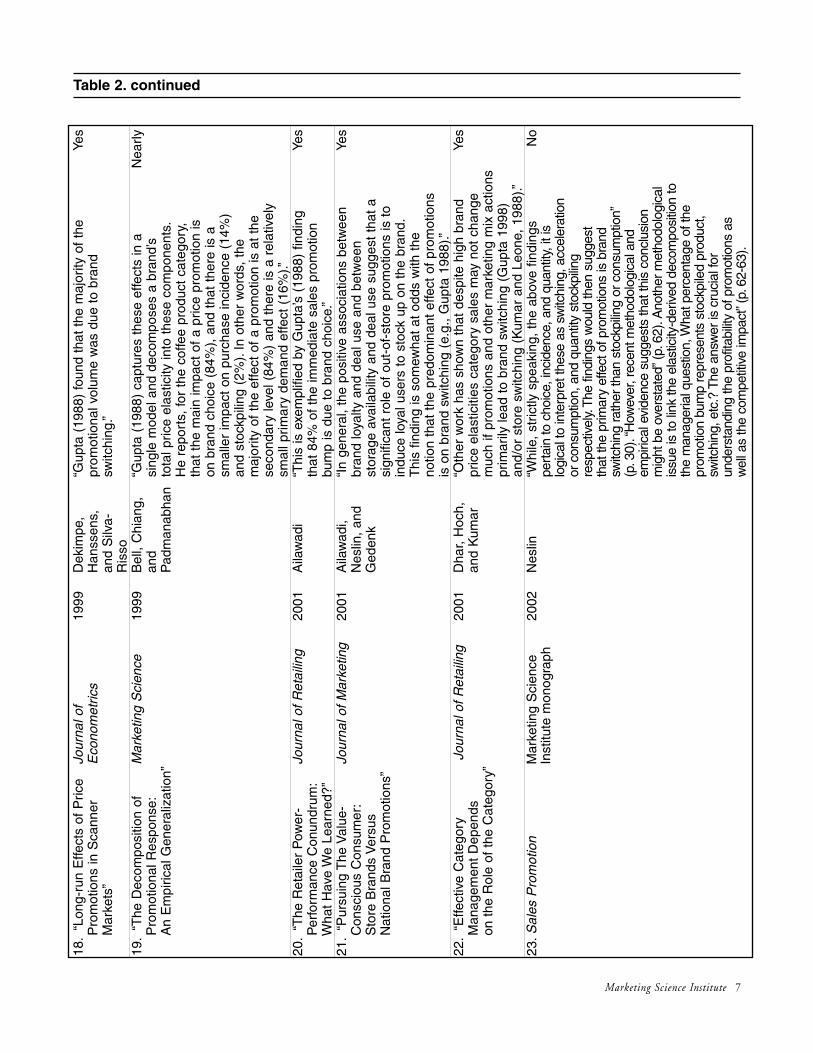
A common interpretation of this decomposition of a promotional elasticity is that if abrand gains 100 units during a promotion, and 74 percent of the sales elasticity isattributable to brand switching, the other brands in the category (are estimated to)lose 74 units. An important point of our paper is that the elasticity decompositiondoes not allow the results to be interpreted in terms of unit sales: other brands lose farless than 74 units. To assess how widespread the misinterpretation is in the marketingliterature, we conducted a review via the Web of Science (Institute for ScientificInformation 2002) and found 145 references to Gupta (1988). Of these, we were ableto access 135 articles. Twenty-three of these made direct reference to the decomposi-tion of promotional response. In Table 2 we list these articles along with the relevanttext extracted from the papers. We find that 16 of the 23 articles (70 percent) incor-rectly interpret Gupta’s decomposition, i.e., the interpretation explicitly refers to incre-mental sales volume resulting from a promotion. Four studies do not literally interpretthe decomposition in this way, although they nearly do so (studies 7, 9, 13, and 19).Only Bucklin, Gupta, and Siddarth (1998) and Kim and Staelin (1999) emphasizethat the correct interpretation is in terms of elasticities, although they do not mentionthat a unit sales effect decomposition might be different. Neslin (2002) raises theimportant question of whether the elasticity decomposition is interpretable in terms ofpercentages with respect to a promotional sales bump.


Table 1. Elasticity Decomposition Results

Study1 Category2 “Secondary “Primary Demand Effect”Demand Effect”

Brand Timing QuantitySwitching Acceleration Acceleration

Gupta (1988) Coffee .84 .14 .02

Chiang (1991) Coffee (feature) .81 .13 .06 Coffee (display) .85 .05 .10

Chintagunta (1993) Yogurt .40 .15 .45

Bucklin, Gupta, and Siddarth Yogurt .58 .19 .22(1998)

Bell, Chiang, and Margarine .94 .06 .00Padmanabhan (1999) Soft drinks .86 .06 .09

Sugar .84 .13 .03Paper towels .83 .06 .11Bathroom tissue .81 .04 .15Dryer softeners .79 .01 .20Yogurt .78 .12 .09Ice cream .77 .19 .04Potato chips .72 .05 .24Bacon .72 .20 .08Liquid detergents .70 .01 .30Coffee .53 .03 .45Butter .49 .42 .09

Average .74 .11 .15

1All studies are based on household data.2Different studies may find different decomposition percentages for the same category due to model differences, data differences, and so

forth.

In this paper we demonstrate that the decomposition of the promotional elasticitydoes not imply an equivalent decomposition of unit sales increases. Instead we findthat the elasticity decomposition reported in the literature translates to a unit salesdecomposition in which the cross-brand component is much smaller than 74 per-cent. We clarify the interpretation of an elasticity decomposition and we show howit can be transformed into a decomposition of unit sales effects. The latter isinstructive for researchers who use models of purchase incidence, brand choice,and quantity, because there is no straightforward unit sales decomposition directlyavailable from those models. Since the literature includes many elasticity decompo-sition results, and since an elasticity decomposition is the common approach forhousehold models, our transformation can be applied to derive substantively usefulresults from models of household data. We show that the transformation of elastic-ity decomposition to unit sales decomposition provides a very different assessmentof the attractiveness of a sales promotion activity. It also changes the ordering ofproduct categories in Bell, Chiang, and Padmanabhan (1999) in terms of relativedesirability for sales promotion based on the fraction of secondary demand effects.

4 Marketing Science Institute


Table 2. Interpretation of Elasticity Decomposition Result in Gupta (1988)A

rtic

le T

itle

Jou

rnal

Year

Au

tho

r(s)

Rel

evan

t Tex

t E

xtra

cted

fro

m A

rtic

leIn

terp

rete

d a

sC

on

trib

uti

on

to

Un

it S

ales

Eff

ect?

1.“I

mpa

ct o

f S

ales

Pro

mot

ion

Jour

nal o

f Mar

ketin

g19

88G

upta

“The

res

ults

indi

cate

tha

t m

ore

than

Yes

on W

hen,

Wha

t, an

d H

ow

Res

earc

h84

% o

f th

e sa

les

incr

ease

due

to

Muc

h to

Buy

”2.

“Sal

es P

rom

otio

n:T

he

Mar

ketin

gLe

tters

1990

Bla

ttber

g “T

he g

ener

al c

onse

nsus

app

ears

to

be t

hat

bran

d

Y

esLo

ng a

nd t

he S

hort

of

It”an

d N

eslin

switc

hing

is a

maj

or s

ourc

e of

vol

ume

(due

to

sale

spr

omot

ions

)....

Gup

ta (

1988

) fo

und

that

sw

itchi

ngac

coun

ted

for

84%

of

the

incr

ease

in c

offe

e br

and

sale

s ge

nera

ted

by p

rom

otio

n.P

uttin

g to

geth

erth

e fa

cts

that

sal

es p

rom

otio

ns g

ener

ate

dram

atic

imm

edia

te s

ales

incr

ease

s an

d th

at b

rand

switc

hing

acc

ount

s fo

r a

larg

e pe

rcen

tage

of

this

incr

ease

, w

e ca

n co

nclu

de t

hat

sale

s pr

omot

ions

3.“A

sses

sing

Pur

chas

e M

arke

ting

Sci

ence

1990

Whe

at a

nd“G

upta

(19

98)

finds

tha

t br

and

switc

hing

Yes

Tim

ing

Mod

els—

Whe

ther

or

M

orris

on

acco

unts

for

mos

t of

the

sal

es in

crea

se d

ue t

o N

ot I

s P

refe

rabl

e to

Whe

n”pr

omot

ion,

whi

le s

tock

pilin

g ac

coun

ts fo

r

only

2%

.”4.

“Det

erm

inin

g In

terb

rand

Jo

urna

l of M

arke

ting

1991

Buc

klin

and

“O

ur a

ppro

ach

does

not

cur

rent

ly in

corp

orat

eYe

sS

ubst

ituta

bilit

y T

hrou

gh

Res

earc

hS

riniv

asan

quan

tity

effe

cts

of p

rice

prom

otio

ns s

uch

asS

urve

y M

easu

rem

ent

ofpu

rcha

se a

ccel

erat

ion

and

stoc

kpili

ng.(

The

seC

onsu

mer

Pre

fere

nce

effe

cts

in t

he c

offe

e ca

tego

ry a

re e

stim

ated

by

Str

uctu

res”

Gup

ta 1

988

to b

e ab

out

16%

of

the

varia

tion

in b

rand

vol

ume.

)”5.

“A S

imul

tane

ous

App

roac

h M

arke

ting

Sci

ence

1991

Chi

ang

“The

se r

esul

ts a

re s

imila

r to

the

one

s ob

tain

edYe

sto

the

Whe

ther

, Wha

t, an

d by

Gup

ta (

1998

, p.

352)

, w

here

84%

of

the

How

Muc

h to

Buy

Que

stio

ns”

incr

ease

is a

ttrib

uted

to

bran

d sw

itchi

ng,

14%

by

pur

chas

e tim

e ac

cele

ratio

n an

d 2%

by

incr

ease

s in

qua

ntity

.”6.

“Sal

es R

espo

nse

of

Jour

nal o

f Adv

ertis

ing

1992

Gre

co a

nd

“In

a st

udy

of t

he im

pact

of

pric

e an

d di

spla

y Ye

sE

lder

ly C

onsu

mer

s to

R

esea

rch

Sw

ayne

prom

otio

ns o

n co

ffee,

Gup

ta (

1988

) P

oint

-of-

Pur

chas

e un

ders

core

d th

e im

port

ance

of

bran

d-sw

itchi

ngA

dver

tisin

g”be

havi

or b

y pr

ovid

ing

empi

rical

evi

denc

e fr

omsc

anne

r pa

nel d

ata

that

indi

cate

d m

ore

than

84 p

erce

nt o

f th

e sa

les

impa

ct d

ue t

o pr

omot

ion

com

es f

rom

bra

nd-s

witc

hing

as

oppo

sed

to

purc

hase

tim

e ac

cele

ratio

n or

sto

ckpi

ling.

”7.

“Asy

mm

etric

Res

pons

e to

Jo

urna

l of

1992

Kris

hnam

urth

i,“G

upta

(19

88)

finds

tha

t a

sign

ifica

nt p

ropo

rtio

nN

early

Pric

e in

Con

sum

er B

rand

C

onsu

mer

Res

earc

hM

azum

dar,

of b

rand

sw

itchi

ng in

cof

fee

purc

hase

isC

hoic

e an

d P

urch

ase

and

Raj

prom

otio

n in

duce

d.”

Qua

ntity

Dec

isio

ns”

8.“A

Mod

el fo

r O

ptim

izin

g th

e Jo

urna

l of B

usin

ess

1994

Ali,

Jol

son,

“A

n em

piric

al a

naly

sis

of I

RI

scan

ner

pane

l dat

aYe

sR

efun

d V

alue

in R

ebat

e R

esea

rch

and

Dar

mon

sugg

ests

tha

t br

and

switc

hing

rat

her

than

Pro

mot

ions

”pu

rcha

se a

ccel

erat

ion

acco

unts

for

mos

t of

the

incr

emen

tal s

ales

due

to

prom

otio

n (G

upta

198

8).”

prom

otio

ns c

omes

fro

m b

rand

sw

itchi

ng.”

a re

stro

ngly

as s

ocia

ted

with

bra

nd s

witc

hing

. ”

Table 2. continued9.

“Con

text

ual a

nd T

empo

ral

Jour

nal o

f Mar

ketin

g19

94R

ajen

dran

“For

sca

nner

dat

a on

cof

fee,

Gup

ta (

1988

) fo

und

Nea

rlyC

ompo

nent

s of

Ref

eren

ce

and

Telli

sth

at p

rice

disc

ount

s ha

d on

ly a

sm

all e

ffect

on

Pric

e”co

nsum

ers’

timin

g an

d qu

antit

y of

pur

chas

es b

uta

stro

ng e

ffect

on

bran

d ch

oice

s;th

eref

ore,

pric

edi

ffere

nces

cou

ld le

ad c

onsu

mer

s to

sw

itch

bran

dsm

ore

than

cha

nge

how

muc

h or

whe

n th

ey b

uy.”

10.

“The

Effe

ct o

f B

rand

Jour

nal o

f Ret

ailin

g19

95K

aran

de a

nd

“Als

o, G

upta

(19

88)

show

ed t

hat

84%

Ye

s C

hara

cter

istic

s an

d R

etai

ler

Kum

arof

the

sal

es in

crea

se d

ue t

o pr

omot

ion

com

es

Pol

icie

s on

Res

pons

e to

from

bra

nd s

witc

hing

.The

refo

re it

is im

port

ant

Ret

ail P

rice

Pro

mot

ions

:to

stu

dy t

he e

ffect

of

reta

iler

polic

ies

onIm

plic

atio

ns fo

r R

etai

lers

”pr

omot

iona

l cro

ss-p

rice

elas

ticiti

es.”

11.

“Do

Hou

seho

ld S

cann

er

Jour

nal o

f Mar

ketin

g19

96G

upta

,“T

he im

port

ance

of

bran

d ch

oice

is u

nder

scor

edYe

s

Dat

a P

rovi

de R

epre

s-R

esea

rch

Chi

ntag

unta

, by

Gup

ta’s

(19

88)

findi

ng t

hat

bran

d sw

itchi

ngen

tativ

e In

fere

nces

fro

m

Kau

l, an

d ac

coun

ts fo

r 84

% o

f th

e ov

eral

l sal

es in

crea

ses

Bra

nd C

hoic

es:A

W

ittin

kdu

e to

pro

mot

ions

in t

he c

offe

e ca

tego

ry.”

Com

paris

on w

ith S

tore

Dat

a”12

.“B

reed

ing

Com

petit

ive

Man

agem

ent S

cien

ce19

97M

idgl

ey,

“Ind

eed,

Gup

ta (

1988

), in

stu

dyin

g co

nsum

er

Yes

Str

ateg

ies”

Mar

ks,

and

pane

l dat

a fr

om t

he s

ame

time,

con

clud

ed

Coo

per

that

incr

ease

d sa

les

from

cof

fee

prom

otio

nsca

me

mor

e fr

om b

rand

sw

itchi

ng t

han

from

forw

ard

buyi

ng o

r st

ockp

iling

.”13

.“W

hen

and

Wha

t to

Buy

:Jo

urna

l of F

orec

astin

g19

98G

uada

gni a

nd

“In

an im

port

ant

pape

r, G

upta

(19

88)

brea

ks

Nea

rlyA

Nes

ted

Logi

t M

odel

Littl

eth

e pu

rcha

se p

roce

ss d

own

into

thr

ee s

epar

ate

of C

offe

e P

urch

ase”

subp

roce

sses

:bra

nd c

hoic

e, q

uant

ity s

elec

ted,

and

inte

rpur

chas

e tim

ing.

...G

upta

’s p

aper

als

opr

ovid

es a

use

ful a

naly

sis

of t

he in

crem

enta

l sal

esin

duce

d by

pur

chas

e ac

cele

ratio

n an

d st

ockp

iling

.”14

.“S

imila

ritie

s in

Cho

ice

Mar

ketin

g S

cien

ce19

98A

insl

ie a

nd

“At

leas

t fo

r th

e ca

se o

f pr

ice,

it h

as b

een

Yes

Beh

avio

r ac

ross

Pro

duct

R

ossi

docu

men

ted

in t

he li

tera

ture

tha

t th

e lio

n’s

Cat

egor

ies”

shar

e of

res

pons

e is

in t

he c

hoic

e as

opp

osed

to

qua

ntity

or

inci

denc

e de

cisi

ons

(Gup

ta 1

998)

.”15

.“D

eter

min

ing

Seg

men

tatio

nJo

urna

l of M

arke

ting

1998

Buc

klin

, “T

he o

vera

ll pr

ice

elas

ticity

can

be

deco

mpo

sed

No

in S

ales

Res

pons

e ac

ross

R

esea

rch

Gup

ta,

and

into

the

sum

of

choi

ce,

inci

denc

e, a

nd q

uant

ityC

onsu

mer

Pur

chas

e S

idda

rth

elas

ticiti

es fo

r th

at s

egm

ent

(e.g

., G

upta

198

8,

Beh

avio

rs”

App

endi

x B

).”16

.“M

arke

ting

Res

earc

h:Jo

urna

l of t

he A

cade

my

1999

Mal

hotr

a,

“The

se r

esul

ts s

erve

to

clar

ify e

arlie

r fin

ding

s Ye

sA

Sta

te-o

f-th

e-A

rt R

evie

w

of M

arke

ting

Sci

ence

Pet

erso

n, a

ndth

at m

ore

than

84

perc

ent

of t

he s

ales

incr

ease

and

Dire

ctio

ns fo

r th

e K

leis

erdu

e to

pro

mot

ion

com

es f

rom

bra

nd s

witc

hing

,Tw

enty

-Firs

t C

entu

ry”

whi

le p

urch

ase

acce

lera

tion

in t

ime

acco

unts

for

less

tha

n 14

per

cent

, w

here

as s

tock

pilin

gdu

e to

pro

mot

ion

acco

unts

for

less

tha

n 2%

of t

he s

ales

incr

ease

(G

upta

198

8).”

17.

“Man

ufac

ture

r A

llow

ance

s M

arke

ting

Sci

ence

1999

Kim

and

“G

upta

(19

98)

estim

ates

tha

t 85

% o

f a

bran

d’s

No

and

Ret

aile

r P

ass-

Thr

ough

S

tael

inpr

omot

iona

l ela

stic

ity is

due

to

bran

d sw

itchi

ng

Rat

es in

a C

ompe

titiv

e w

hile

the

res

t is

due

to

chan

ges

in t

he q

uant

ity

Env

ironm

ent”

norm

ally

pur

chas

ed o

r in

the

fre

quen

cy o

f pu

rcha

se,

i.e.,

purc

hase

inci

denc

e.”



Table 2. continued18

.“L

ong-

run

Effe

cts

of P

rice

Jour

nal o

f19

99D

ekim

pe,

“Gup

ta (

1988

) fo

und

that

the

maj

ority

of

the

Yes

Pro

mot

ions

in S

cann

er

Eco

nom

etric

sH

anss

ens,

pr

omot

iona

l vol

ume

was

due

to

bran

d M

arke

ts”

and

Silv

a-sw

itchi

ng.”

Ris

so19

.“T

he D

ecom

posi

tion

of

Mar

ketin

g S

cien

ce19

99B

ell,

Chi

ang,

“Gup

ta (

1988

) ca

ptur

es t

hese

effe

cts

in a

N

early

Pro

mot

iona

l Res

pons

e:an

d si

ngle

mod

el a

nd d

ecom

pose

s a

bran

d’s

An

Em

piric

al G

ener

aliz

atio

n”P

adm

anab

han

tota

l pric

e el

astic

ity in

to t

hese

com

pone

nts.

He

repo

rts,

for

the

coffe

e pr

oduc

t ca

tego

ry,

that

the

mai

n im

pact

of

a pr

ice

prom

otio

n is

on b

rand

cho

ice

(84%

), a

nd t

hat

ther

e is

asm

alle

r im

pact

on

purc

hase

inci

denc

e (1

4%)

and

stoc

kpili

ng (

2%).

In o

ther

wor

ds,

the

maj

ority

of

the

effe

ct o

f a

prom

otio

n is

at

the

seco

ndar

y le

vel (

84%

) an

d th

ere

is a

rel

ativ

ely

smal

l prim

ary

dem

and

effe

ct (

16%

).”20

.“T

he R

etai

ler

Pow

er-

Jour

nal o

f Ret

ailin

g20

01A

ilaw

adi

“Thi

s is

exe

mpl

ified

by

Gup

ta’s

(19

88)

findi

ngYe

s

P

erfo

rman

ce C

onun

drum

:th

at 8

4% o

f th

e im

med

iate

sal

es p

rom

otio

n W

hat

Hav

e W

e Le

arne

d?”

bum

p is

due

to

bran

d ch

oice

.”21

.“P

ursu

ing

The

Val

ue-

Jour

nal o

f Mar

ketin

g20

01A

ilaw

adi,

“In

gene

ral,

the

posi

tive

asso

ciat

ions

bet

wee

n Ye

sC

onsc

ious

Con

sum

er:

Nes

lin,

and

bran

d lo

yalty

and

dea

l use

and

bet

wee

n S

tore

Bra

nds

Ver

sus

Ged

enk

stor

age

avai

labi

lity

and

deal

use

sug

gest

tha

t a

Nat

iona

l Bra

nd P

rom

otio

ns”

sign

ifica

nt r

ole

of o

ut-o

f-st

ore

prom

otio

ns is

to

indu

ce lo

yal u

sers

to

stoc

k up

on

the

bran

d.T

his

findi

ng is

som

ewha

t at

odd

s w

ith t

he

notio

n th

at t

he p

redo

min

ant

effe

ct o

f pr

omot

ions

is

on

bran

d sw

itchi

ng (

e.g.

, G

upta

198

8).”

22.

“Effe

ctiv

e C

ateg

ory

Jour

nal o

f Ret

ailin

g20

01D

har,

Hoc

h,

“Oth

er w

ork

has

show

n th

at d

espi

te h

igh

bran

d Ye

sM

anag

emen

t D

epen

ds

and

Kum

arpr

ice

elas

ticiti

es c

ateg

ory

sale

s m

ay n

ot c

hang

e on

the

Rol

e of

the

Cat

egor

y”m

uch

if pr

omot

ions

and

oth

er m

arke

ting

mix

act

ions

prim

arily

lead

to

bran

d sw

itchi

ng (

Gup

ta 1

998)

an

d/or

sto

re s

witc

hing

(K

umar

and

Leo

ne,

1988

).”23

.Sal

es P

rom

otio

nM

arke

ting

Sci

ence

20

02N

eslin

“Whi

le,

stric

tly s

peak

ing,

the

abo

ve f

indi

ngs

No

Inst

itute

mon

ogra

phpe

rtai

n to

cho

ice,

inci

denc

e, a

nd q

uant

ity, i

t is

logi

cal t

o in

terp

ret t

hese

as

switc

hing

, acc

eler

atio

n or

con

sum

ptio

n, a

nd q

uant

ity s

tock

pilin

gre

spec

tivel

y.T

he fi

ndin

gs w

ould

then

sug

gest

that

the

prim

ary

effe

ct o

f pro

mot

ions

is b

rand

switc

hing

rath

er th

an s

tock

pilin

g or

con

sum

ptio

n”(p

.30)

.“H

owev

er, r

ecen

t met

hodo

logi

cal a

nd

empi

rical

evi

denc

e su

gges

ts th

at th

is c

oncl

usio

nm

ight

be

over

stat

ed”(

p.62

).A

noth

er m

etho

dolo

gica

l is

sue

is to

link

the

elas

ticity

-der

ived

dec

ompo

sitio

n to

the

man

ager

ial q

uest

ion,

Wha

t per

cent

age

of th

epr

omot

ion

bum

p re

pres

ents

sto

ckpi

led

prod

uct,

switc

hing

, etc

.? T

he a

nsw

er is

cru

cial

for

unde

rsta

ndin

g th

e pr

ofita

bilit

y of

pro

mot

ions

as

wel

l as

the

com

petit

ive

impa

ct”(

p.62

-63)

.


We proceed as follows. We first review and clarify the elasticity decompositionbased on household data. We show mathematically how the elasticity decomposi-tion may be transformed to a unit sales effect decomposition. We use the resultingtransformation equations to infer unit sales effects from elasticity results for threecategories for which we estimate household-level decomposition models (Study 1).We also present an equation that approximates the fraction of secondary demandeffects if only aggregate elasticities are available. We apply the latter equation to theelasticity decomposition results in Bell, Chiang, and Padmanabhan (1999) (Study2). Both studies provide convincing evidence that far less than 74 percent of theunit sales increase due to promotions comes from cross-brand sales. In the finalsection, we present managerial implications, conclusions, and directions for futureresearch.


Transforming ElasticityDecomposition to Unit SalesDecomposition

For the decomposition of sales promotion effects into secondary and primarydemand effects based on elasticities, we start with the key equation underlying thisdecomposition:1

Sj = P(I)P(Cj | I)Qj (1)

where:

Sj = expected unit sales of brand j

{ I } = household makes a category purchase (purchase incidence)

{ Cj } = household chooses brand j

P(I) = probability of category purchase incidence

P(Cj | I) = probability of choice of brand j, given purchase incidence

Qj = quantity bought given purchase of brand j.

Define Dj as the actual price relative to the regular price for brand j on the pur-chase occasion. Based on Equation 1, the elasticity of brand sales with respect toDj is given by the chain rule for the product of functions:

(2)

or

(3)

where:

= sales elasticity of brand j

= elasticity of category purchase incidence with respect to DjjIη

jSη

| | ,j j j j jS I C I Q I Cη η η η= + +

( | )( )

( ) ( | )j

j j j j j j jS

j j j j j j j

S D D P C I D Q DP I

D S D P I D P C I D Qη

∂ ∂ ∂∂= = + +∂ ∂ ∂ ∂


= elasticity of choice probability of brand j, conditional on purchase incidence

= elasticity of purchase quantity, conditional on purchaseincidence and choice of brand j.

Equation 3 shows that the sales elasticity may be additively decomposed into theelasticities of the three components. Using this property, several researchers haveprovided percentage decompositions of the sales elasticity (see Table 1). Across allcategories, the average brand switching component is by far the largest (74 per-cent), followed by purchase quantity (15 percent), and purchase timing (11 per-cent). However, the percentages differ substantially across categories, as also sug-gested by Blattberg, Briesch, and Fox (1995). For example, categories for whichhousehold inventories tend to be modest, such as margarine and ice cream, showrelatively small purchase quantity percentages. For more detail on reasons for dif-ferences across categories and brands, see Bell, Chiang, and Padmanabhan (1999).

Bell, Chiang, and Padmanabhan (1999) use the concept of “primary demandeffect” for the sum of the purchase incidence elasticity and the purchase quantityelasticity. Both elasticities reflect earlier or larger purchases in the category, andresult in consumers having higher inventories and/or increased consumption. Thedistinction between these two types of primary demand effects is only modestlymeaningful for managerial purposes since both may capture stockpiling and con-sumption. Therefore we also combine them into one measure so that the primarydemand fraction out of the total effect is (see also Bell, Chiang, and Padmanabhan1999):

(4)

The secondary demand effect is the brand choice elasticity, and it reflects switchingbehavior. The fraction of secondary demand effects based on the elasticities is:

(5)

Gupta (1988) provides the following example of a feature-and-display elasticity forFolgers 16-ounce coffee: ηS = .248; ηC|I = .210; ηI = .034; and ηQ|C,I = .004.Hence, PDelast = (.034 + .004/.248 = .16 and SDelast = .210/.248 = .84.

Gupta interpreted this fraction to mean that the vast majority of the sales effect isdue to brand switching: “The results indicate that more than 84% of the salesincrease due to promotions comes from brand switching . . .” (1988, p. 342). Thisinterpretation dominates the marketing literature, as we show in Table 2. We nowdemonstrate the correct interpretation.2 Suppose Folgers 16-ounce has an initialchoice probability of 18 percent (i.e., its overall market share is 18 percent). Andsuppose the initial purchase incidence probability in a given week is 20 percentwhile the number of purchase occasions is 1,000. Then category sales in that week

|

elast,jSD j

j

C I

S

η

η=

| ,

elast,jPD j j j

j

I Q I C

S

η η

η

+=

| ,j jQ I Cη

|jC Iη


are 200 units, sales of Folgers 16-ounce are 36 units, and sales of the other brandsare 164 units. If there is a feature and display, and ηS = .248, sales of Folgers 16-ounce change to 1.248 * 36 = 45.2 units. Where does this increase of 9.2 unitscome from? The incidence probability goes up to 1.034 * 20% = 20.7%. Thechoice probability for Folgers 16-ounce increases to 1.210 * 18% = 21.8%, so thatthe other brands together have 78.2 percent choice probability. Sales of the otherbrands equal .207 * .782 * 1,000 = 161.8 units, representing a 2.2 unit decline.This decline represents only 24.3 percent of the 9.2 unit sales increase for Folgers16-ounce.

The key difference between the percentage attributable to brand switching accord-ing to the elasticity decomposition (84 percent) and the unit sales decomposition(24 percent) lies in the way the approaches treat the category expansion inducedby the increase in the purchase incidence probability. The elasticity decompositionholds the category constant to assess the brand switching fraction (Bucklin, Gupta,and Siddarth 1998, p. 196). If we hold the category constant at 200 units, thenunder this promotion the other brands together sell .782 * 200 = 156.4 units. Thisrepresents a gross decline of 7.6 units from the original sales of 164 units, which isexactly 84 percent of the 9.2 unit sales increase for Folgers 16-ounce. However,another relevant component is the increase in the purchase incidence probability.The other brands gain 5.3 units from this category expansion, so that their netsales loss equals (approximately) 2.2 units. This is the number used in the unitsales decomposition to yield 24.3 percent of the sales increase. We argue that thisnet decrease in sales of the non-promoted brands is the bottom-line quantity ofinterest to retailers, to brand managers of the non-promoted brands, and to brandmanagers of the promoted brands, since it represents the sales loss for the non-pro-moted brands after all calculations have been made. In the literature, the net unitsales interpretation of the elasticity decomposition dominates, as indicated in Table2, although the numbers represent a gross sales loss. As a consequence, we needequations to transform the elasticity decomposition into a net unit sales effectdecomposition.

To achieve this, we start with expressions of unit sales and define the followingidentity equation:3

(6)

This equation says that own-brand sales of brand j equals category sales (summa-tion across all J brands) minus cross-brand sales on the same occasion (summationacross all J brands except for brand j). We now consider infinitesimal changes inthe sales promotion variable, i.e., temporary price cuts, since point elasticities arealso based on such changes.4 An infinitesimal temporary price reduction for brandj is denoted by ∂Dj. The own-brand sales effect due to this promotion is ∂Sj / ∂Dj.

5

Using Equation 6, we can write this as the effect on category sales minus the effecton cross-brand sales:

1 1

J J

j k kk k

k j

S S S= =

≠

= −∑ ∑


(7)

We now divide both sides of Equation 7 by the own-brand sales effect (∂Sj | ∂Dj).The left-hand side then equals 1, and the right-hand side consists of two terms.The first term represents the fraction of the own-brand sales increase due to prima-ry demand effects, since it expresses the effect of the promotion on category salesas a fraction of the own-brand sales effect:

(8)

The second term represents the fraction of the own-brand unit sales increase dueto secondary demand effects (decreases in unit sales of other brands), since it is theratio of minus the cross-brand sales effect (loss) over the own-brand sales change:6

(9)

The fractions of primary and secondary demand effects sum to 1 by definition.

We now show the relationship between the elasticity decomposition (equations 4and 5) and unit sales decomposition (equations 8 and 9). Starting with the elastici-ty decomposition on a purchase occasion, we obtain (see the appendix) the follow-ing expressions for SDsales,j and PDsales,j:

(10)

and

PDsales, j = 1 – SDsales, j (11)

where is the elasticity of category purchase incidence, is the elasticity ofchoice probability of brand k when j is promoted, conditional on purchase inci-dence, and is the elasticity of purchase quantity of brand j, conditional onpurchase incidence and choice of brand j, each with respect to Dj.

In Study 1 (to follow), we apply equations 10 and 11, which are central to thispaper, to three household-level datasets. The intuition behind Equation 10 is easierto see if we use a simplified version of Equation 10 ([A2] in the appendix) that

jjQη

|kjC IηjIη

++

+−= ∑

≠= )|(

)|(SD

1 |

|

sales, ICP

ICP

Q

Q

j

k

j

kJ

jkk QICI

ICI

j

jjjjj

kjj

ηηηηη

1

sales,

/

SD Fraction Secondary Demand Effects in Sales of brand /

J

k jkk j

jj j

S D

jS D

=≠

−∂ ∂

= =∂ ∂

∑

1sales,

/PD Fraction Primary Demand Effects in Sales of brand

/

k jk

jj j

S Dj

S D=

∂ ∂= =

∂ ∂

∑

1 1

/ / /J J

j j k j k jk k

k j

S D S D S D= =

≠

∂ ∂ = ∂ ∂ − ∂ ∂∑ ∑


obtains if we assume that the non-promotional purchase quantities are equal acrossbrands (Qj = Qk = Q∀j, k):

(12)

Equation 12 shows that to obtain the fraction of secondary demand effects in netunit sales, we have to subtract from the gross elasticity-based fraction an amount,A, which is the fraction of the sales elasticity attributable to the incidence elasticitytimes the inverse of the odds of conditionally choosing brand j:

Since A is ordinarily a positive quantity, Equation 12 shows that in the unit salesdecomposition, the secondary demand effect fraction will decrease relative to theelasticity decomposition.

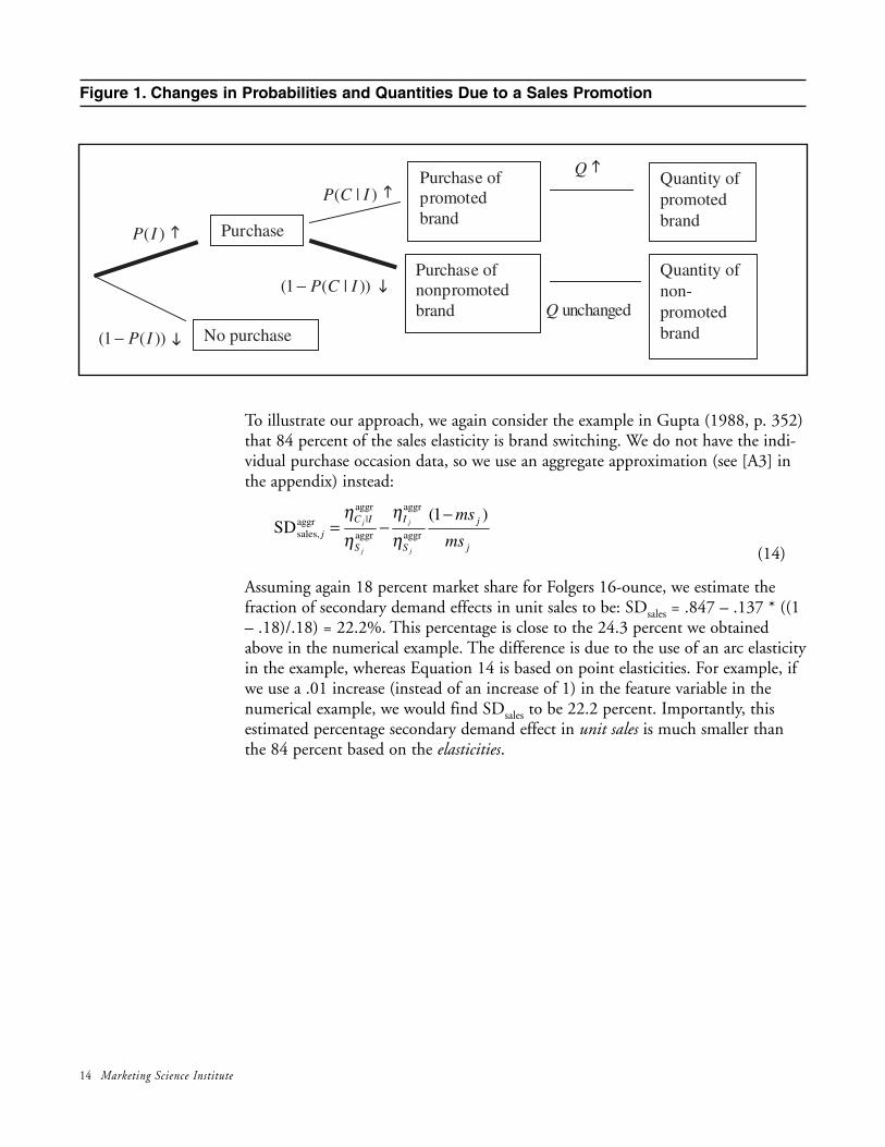
The change in sales of non-promoted brands consists of two parts: a positive partdue to an increase in the category purchase incidence probability, and a negativepart due to decreased conditional choice probabilities. This is illustrated in Figure1 by the two bold lines. The first bold line shows that a temporary price cut for abrand may increase the purchase incidence probability. A large part of this favorsthe promoted brand. However, the non-promoted brands may also benefit accord-ing to the model specification. That is, even though their conditional choice prob-abilities tend to decrease, other brands may experience a partly offsetting gain fromthe increased purchase incidence probability. The quantity A reflects this gain.

A mathematical explanation for the quantity A is that due to the promotion forbrand j, there is an increase in the overall purchase incidence probability of size

. Keeping the conditional choice probability and purchase quantity con-stant, this leads to a sales increase of the non-promoted brands of size

. When we express this sales increase relative to the salesincrease of brand j, we obtain A:

(13)

AICP

ICP

QICPIP

QICPIP

jS

jI

jS

jI

j

j

j

j ≡−

=−

)|(

))|(1(

)|()(

))|(1)((

ηη

ηη

QICPIP jI j))|(1)(( −η

)(IPjIη

(1 ( | ))

( | )j

j

I j

S j

P C IA

P C I

η

η−

=

AICP

ICPj

j

j

S

I

S

IC

j

j

j

j

j −=−

−= elast,

|

sales, SD)|(

))|(1(SD

ηη

ηη


Figure 1. Changes in Probabilities and Quantities Due to a Sales Promotion

To illustrate our approach, we again consider the example in Gupta (1988, p. 352)that 84 percent of the sales elasticity is brand switching. We do not have the indi-vidual purchase occasion data, so we use an aggregate approximation (see [A3] inthe appendix) instead:

(14)

Assuming again 18 percent market share for Folgers 16-ounce, we estimate thefraction of secondary demand effects in unit sales to be: SDsales = .847 – .137 * ((1– .18)/.18) = 22.2%. This percentage is close to the 24.3 percent we obtainedabove in the numerical example. The difference is due to the use of an arc elasticityin the example, whereas Equation 14 is based on point elasticities. For example, ifwe use a .01 increase (instead of an increase of 1) in the feature variable in thenumerical example, we would find SDsales to be 22.2 percent. Importantly, thisestimated percentage secondary demand effect in unit sales is much smaller thanthe 84 percent based on the elasticities.

j

j

S

I

S

IC

j ms

ms

j

j

j

j)1(

SDaggr

aggr

aggr

aggr|aggr

sales,

−−=

ηη

ηη

unchanged Q

Q

)(IP

− ))|(1( ICP

)|( ICP

− ))(1( IP No purchase

Purchase

Purchase of promoted brand

Purchase of nonpromoted brand

Quantity ofpromotedbrand

Quantity ofnon-promotedbrand


Study 1: Brand Switching Basedon Household Data

We use the transformations to obtain unit sales decompositions from three house-hold panel datasets: yogurt, tuna, and sugar. The yogurt data consist of 28,720store visits by 223 households in Springfield, Missouri. Of these trips, 2,424resulted in purchases of one of the following four brands: Yoplait, Dannon, WeightWatchers, and Hiland. We model purchase incidence, brand choice, and purchasequantity. The model is essentially the one in Bucklin, Gupta, and Siddarth(1998)—a latent class model with nested logit specification for incidence andbrand choice, and a truncated-at-1 Poisson model for quantity. We find a three-segment model fits the yogurt data best.

The tuna data consist of 17,771 store visits by 270 households in Sioux Falls,South Dakota. Of these trips, 1,740 resulted in purchases of one of the followingtwo brands: Chicken of the Sea and StarKist. The product is a 6.5-ounce can ofwater- or oil-based chunky tuna. We use the same model as for yogurt, and findthat a three-segment model fits these data best as well. The sugar data consist of17,492 store visits by 266 households in Springfield, Missouri. Of these trips,1,824 resulted in purchases of one of the following two brands: private label andC&H. These are the two largest brands of 5-lb. bags of sugar in the market. Usingthe same model as for yogurt and tuna, we also find here that a three-segmentmodel fits the data best.

We summarize the results in Table 3. For yogurt, the fraction of secondary demandbased on elasticities (Equation 5) is on average .58. However, the fraction of sec-ondary demand based on unit sales effects (Equation 10) is quite a bit lower, .33.The approximate formula (Equation 14) based on aggregate quantities yields .29,which is reasonably close to .33. For tuna, the average elasticity-based secondarydemand fraction is .49, whereas in unit sales it is .22 or, based on the aggregateapproximation, .23. For sugar, the elasticity decomposition attributes .65 to sec-ondary demand, whereas in unit sales it is .45 whether based on individual oraggregate data. We conclude that brand switching contributes far less to the own-brand unit sales effect than what one might believe based on the elasticity decom-position. On average across these three categories, it is only 33 percent, whereasthe elasticity decomposition suggests 57 percent. Further, the aggregate approxima-tion formula provides results close to the average results from the purchase-occa-sion-level transformation. This suggests that we can apply the aggregate approxi-mation formula to published results for which we do not have individual data.


Table 3. Decomposition Results for Household Data

Brand—Yogurt Yoplait Dannon Weight Hiland AverageWatchers

Average purchase incidence elasticity .40 .56 .14 .28 .34Average conditional choice elasticity 1.99 1.79 2.66 2.25 2.17Average conditional quantity elasticity 1.35 1.31 1.30 .91 1.22Total elasticity 3.74 3.65 4.10 3.44 3.73

SDelast (Equation 5) .53 .49 .65 .65 .58

Average SDsales (Equation 10) .33 .31 .40 .28 .33Aggregate SDsales (Equation 14) .30 .27 .32 .27 .29

Market share .31 .41 .10 .18

Brand—Canned Tuna Chicken StarKist Averageof the Sea

Average purchase incidence elasticity .96 .89 .92Average conditional choice elasticity 1.64 1.90 1.77Average conditional quantity elasticity .92 .94Total elasticity 3.52 3.63

SDelast (Equation 5) .47 .49

Average SDsales (Equation 10) .22 .23 .22Aggregate SDsales (Equation 14) .25 .22 .23

Market share .55 .45

Brand—Sugar Control C&H Average

Average purchase incidence elasticity .40 1.19 .80Average conditional choice elasticity 3.82 1.13 2.48Average conditional quantity elasticity .23 .21 .22Total elasticity 4.45 2.53 3.49

SDelast (Equation 5) .86 .45 .65

Average SDsales (Equation 10) .59 .31 .45Aggregate SDsales (Equation 14) .62 .27 .45

Market share .27 .73

.953.74

.51


Study 2: Brand Switching Basedon Published HouseholdDecomposition Results

We now reconsider the decomposition results in Bell, Chiang, and Padmanabhan(1999).7 We reproduce in Table 4 for each product category the fraction of sec-ondary demand elasticity (Bell et al.’s Table 5). Next to those fractions we presentthe fraction of secondary demand unit sales based on Equation 14. The SDsales frac-tions represent share-weighted averages, similar to Bell, Chiang, and Padmanabhan(1999). The differences between columns 2 and 3 are dramatic. On average, thesecondary demand effects fraction based on the elasticity decomposition is .75,whereas it is only .13 based on a unit sales decomposition. However, the number.13 is affected by the negative numbers for ice cream and butter. For these cate-gories, the application of Equation 14 results in negative values of SDsales

. As dis-cussed in note 5, this is a theoretically feasible result. It means that the promotionof one brand of butter or ice cream can stimulate households to also buy non-pro-moted brands. A factor that may contribute to this empirical finding is the possi-ble occurrence of zero inventory for promoted items. The negative result occurs ifthe incidence elasticity is so large that the loss in conditional brand choice is offsetby the gain in category demand.

Table 4. Comparison of Secondary Demand Effects: Elasticity versus Unit Sales

Category SDelast1 SDsales

2 Attractiveness for sales promotion based on elasticity based on unit sales effect

decomposition decompositionMargarine .94 .51 13 13Soft drinks .86 .36 12 9Sugar .84 .34 11 7Paper towels .83 .42 10 11Bathroom tissue .81 .43 9 12Dryer softeners .79 .36 8 10Yogurt .78 .12 7 3Ice cream .77 –1.64 6 1Potato chips .72 .35 5 8Bacon .72 .14 4 4Liquid detergents .70 .31 3 6Coffee .53 .23 2 5Butter .49 –.26 1 2

Overall average .75 .13

Average withoutice cream and butter .77 .33

1 Secondary demand effects based on elasticity decomposition (Bell, Chiang, and Padmanabhan 1999, Table 5)2 Secondary demand effects based on approximate unit sales effect decomposition (Equation 14)


Specifically, the number –1.64 for ice cream means that if one brand promotes andgains 100 units, the other brands together gain 164 units. There are 11 ice creambrands, so on average the 10 other brands gain 16.4 units, not an implausibleresult. For example, the promotion of one brand may trigger consideration of thecategory with positive effects for non-promoted brands if brand preferences arestrong. For butter, –.26 means that if the promoted brand gains 100 units, theother brands together gain 26 units. There are 4 brands, so on average the 3 otherbrands gain 8.7 units.

If these two categories have especially strong brand preferences, they may be sus-ceptible to such cross-brand effects. However, we note that the aggregate formula(Equation 14) is an imperfect approximation of the real fraction based onEquation 10, and any errors may also contribute to this result for ice cream andbutter.

We obtain perhaps a more realistic estimate for the secondary demand fraction byexcluding these two categories. In that case the secondary demand fraction is .33,which happens to be the same as the average across three categories in Table 3.Importantly, no matter how we compute the average in Table 4, brand switchingin unit sales is not nearly as strong as it is in elasticity. For example, the lowest elas-ticity fraction is .49 (butter in column 1), whereas the highest unit sales fraction is.51 (margarine in column 2). The implication is clear: secondary demand effectsare far less important than what has been claimed.

We note that although the ice cream and bacon categories have very similar elastic-ity patterns, the unit sales decompositions are quite different. This result is causedby differences in (average) market shares for the brands in these categories. In theice cream category, there are 11 brands versus 6 in the bacon category. As a conse-quence, the average market share in the ice cream category is much lower, leadingto lower secondary demand effects based on Equation 14. The intuition for thisresult is that, ceteris paribus, there is less switching in a diversified category withmany items, which may be related to the existence of heterogeneous consumerpreferences.


Managerial Implications

The current literature, based on models of household data, suggests that the vastmajority of the sales increase due to promotional activities is attributable to brandswitching (see Table 1). Bell, Chiang, and Padmanabhan (1999) find that on aver-age, across various categories, secondary demand effects account for about 75 per-cent of the sales elasticity. We show that this result does not imply that if a pro-moted brand gains 100 units, the other brands together lose 75 units. To arrive ata substantively interpretable decomposition, we express the results in terms ofcomparable unit sales effects. We find that on average the secondary demand effectis only about one-third of the total unit sales effect. One interpretation of the dif-ference from the elasticity fraction is that our decomposition considers the net salesdecrease of the other brands, whereas the elasticity decomposition considers thegross decrease. That is, the elasticity approach does not account for the fact thatpart of the increased purchase incidence probability favors the non-promotedbrands, according to the model specification. We argue that the net sales decreaseis the bottom-line quantity for managers, since it shows the total result after all cal-culations have been done. Importantly, this same net decrease should be visible orestimable from (store-level) sales data. These findings may help managers reconcileinconsistencies between their own experiences (“there is little switching”) and acad-emic research that suggests brand switching tends to be the predominant source ofthe promotional bump.

The strikingly different brand switching contribution has important implicationsfor manufacturers and retailers. Although the estimated short-term own-brandsales increase is the same, the major source of the increase is different. If three-fourths of the sales effect were due to other brands, retailers might conclude thatpromotional activities provide little benefit. That is, unless promoted items providehigher margins, the vast majority of the effect would simply be a reallocation ofexpenditures by households across items within a category. Manufacturers wouldconclude that most of the effect enhances competition between brands. Instead, wefind that the vast majority of the sales effect consists of primary demand effects.Thus, stockpiling and/or category expansion together appear to be the dominantsources of sales effects due to temporary price cuts. Manufacturers may prefer thegreatest source to be primary demand, assuming that competitors tend to matcheach other’s promotional activities especially if most of the effect is due to brandswitching. Retailers should also prefer primary demand to secondary demandeffects, since store switching is one possible part of the primary demand effect.

Apart from the large difference between the two decompositions in the averageproportion of the sales increase attributable to secondary demand effects, it is use-ful to order product categories according to this proportion. To illustrate, we showin the last two columns of Table 4 the rank order from the most attractive category(lowest fraction of secondary demand effects = 1) to the least attractive category(highest fraction of secondary demand effects = 13), based on the elasticity decom-position in the third column, and based on the unit sales decomposition in the


fourth column.8 We find, for instance, that whereas ice cream is the sixth-most-attractive category for sales promotions based on the elasticity decomposition, it isfirst based on the unit sales effect decomposition. Similarly, yogurt becomes rela-tively much more attractive to promote: instead of seventh it is third, and its brandswitching fraction changes from 78 percent to 12 percent!

Our results may imply that promotions are more attractive for managers than hasbeen assumed so far. There are, however, two other aspects worth considering.First, the extent to which a primary demand effect represents cannibalization offuture sales via stockpiling is an important consideration in the assessment of theeffectiveness of sales promotions. In some product categories a substantial compo-nent of the primary demand increase may represent enhanced consumption(Ailawadi and Neslin 1998; Sun 2001). But in other categories households areunlikely to accelerate consumption (such as for sugar and bathroom tissue), so thatsome primary demand effects may just represent inventory management by house-holds. Second, we note that the long-term effects of promotions have been docu-mented to be detrimental (Mela, Gupta, and Lehmann 1997).


Conclusions and Directions forFuture Research

Our main conclusion is that although the decomposition of sales promotion effectsbased on elasticities is mathematically correct, its commonly used interpretation(see Table 2) is incorrect. We find that secondary demand effects represent, onaverage, a third of the unit sales effect. Our unit sales decomposition answers thequestion: What part of own-brand sales gains due to a sales promotion is attribut-able to losses for other brands, and what part is attributable to primary demandeffects? To accomplish this, the composite term (unit sales effect) and the decom-position terms (primary and secondary demand effects) are expressed in exactly thesame units. The elasticity decomposition is in itself correct, but it must be inter-preted with care: it gives insight in each of the three promotion effects, holding theother two effects constant (Bucklin, Gupta, and Siddarth 1998, p. 196).Researchers who use household data can use the formulas we provide to convertelasticity results into a unit sales effect decomposition. Alternatively, they can con-duct market simulations based on the estimated incidence, choice, and quantityeffects so as to derive unit sales decompositions (cf. Vilcassim and Chintagunta1995).

We note that the unit sales effect decomposition does not restrict the fraction ofsecondary demand effects to lie between 0 and 1. We find in our second study thatthe fraction is negative for two product categories. We do not consider this to be alimitation for two reasons. One, this result just indicates what the elasticity decom-position implies in unit sales terms: other brands may have a net gain in sales fromthe promotion of the focal brand. The unit sales outcome is directly linked to theelasticity result, and, as a consequence, any result that one might consider(im)plausible is due to the (im)plausibility of the elasticity decomposition results.Two, it only occurs for 2 of the 16 datasets analyzed in tables 3 and 4, specificallywhen we had to use an approximation formula (Table 4).

The misinterpretation of the decomposition result that has prevailed for more thana decade in the literature is due to the use of elasticities instead of absolute saleseffects. This observation is similar to claims made by Sethuraman, Srinivasan, andKim (1999). They argue that the use of non-comparable elasticities has led to sup-port for theories of asymmetric switching behavior between brands (Blattberg andWisniewski 1989). That is, this asymmetry may not hold if one uses an absolutemeasure of cross-price effects. Sethuraman, Srinivasan, and Kim (1999) show thatasymmetries in cross-price elasticities tend to favor a high-priced brand because ofscaling effects. Thus, it is clear that elasticities must be interpreted with great careso as to avoid improper comparisons.

One possible direction for future research is to study category differences in thefractions of primary and secondary demand effects measured in unit sales. In addi-tion, it is of interest to explore cross-category effects (Song and Chintagunta 2001)


for promotions. For example, categories may experience asymmetric effects, such asmargarine losing sales to butter but butter not losing to margarine, if an item ineither category is promoted. Another possibility lies in a direct comparison ofhousehold purchase and store sales data. Gupta, Chintagunta, Kaul, and Wittink(1996) compared price elasticities, based on equivalent model specifications. Theyfound that the substantive conclusions did not differ dramatically between the twosources of data, as long as the household data were chosen based on “purchaseselection”. If managers tend to prefer store-level data for decision-making purposes,it would be of interest to see how proper household-model-based decompositionscompare with corresponding store-model-based decompositions. Finally, it wouldbe useful to determine whether the nature of the decomposition of a sales increasedue to promotion matters to manufacturers and retailers. For example, are compet-itive reaction effects sensitive to the secondary demand fraction?


Appendix: Expressions forPrimary and Secondary DemandEffects

We start with the definition of the secondary demand effect in unit sales on a pur-chase occasion:

The numerator equals:

Note that we use the result that the effect of brand j’s promotion on brand k’s con-ditional purchase quantity is zero ( ), since that is the assumption used in

all five major decomposition papers: Gupta (1988), Chiang (1991), Chintagunta(1993), Bucklin, Gupta, and Siddarth (1998), and Bell, Chiang, andPadmanabhan (1999). This assumption is plausible: conditional on choosing anon-promoted brand, the expected purchase quantity is unchanged. It would bestraightforward to allow for non-zero cross-brand quantity effects in the equations,however.

0k

j

Q

D

∂ =∂

|1

1( ) ( ) ( | )

j kj

J

I C I k kk jk j

P I P C I QD

η η=≠

= − +

∑

|1

( | )( )( | ) ( ) 0

j kj

Jk

I k k C I kk j jk j

P C IP IP C I Q P I Q

D Dη η

=≠

= − + +

∑

1 1

( | )( )/ ( | ) ( ) ( ) ( | )

J Jk k

k j k k k kk k j j jk j k j

P C I QP IS D P C I Q P I Q P I P C I

D D D= =≠ ≠

∂ ∂∂− ∂ ∂ = − + + ∂ ∂ ∂ ∑ ∑

1

sales,

/

SD /

J

k jkk i

jj j

S D

S D

=≠

− ∂ ∂

=∂ ∂

∑


The denominator equals:

Hence the ratio equals:

(A1)

Equation A1 represents the exact definition, applicable to each purchase occasionseparately. If we have only aggregate elasticities and market shares, we need as anintermediate step a version in which we assume that . ThenEquation A1 reduces to:

(A2)

Proof:

1

1 ( | ) ( | )1

( | ) ( | )j

j j

JI j k

jtkS j S j jtk j

P C I P C ID

P C I P C I D

ηη η =

≠

− ∂= + ∂ ∑

|

1 1

( | ) ( | )

( | ) ( | )j kj

j j

J JI C Ik k

k kS j S jk j k j

P C I P C I

P C I P C I

η ηη η= =

≠ ≠

= − +

∑ ∑

| ( | )

( | )j kj

j

JI C I k

i j S j

P C I

P C I

η ηη≠

+ = −

∑

|

sales,1 |

( | )SD

( | )j kj

j jj jj

JI C I k k

jk I C I Q j jk j

Q P C I

Q P C I

η ηη η η=

≠

+ = − + +

∑

)|(

))|(1(SD

|

sales, ICP

ICP

j

j

S

I

S

IC

j

j

j

j

j−

−=ηη

ηη

kjQQQ kj , ∀==

++

+−= ∑

≠= )|(

)|(SD

1 |

|

sales, ICP

ICP

Q

Q

j

k

j

kJ

jkk QICI

ICI

j

jjjjj

kjj

ηηηηη

|

( ) ( | ) 1( ) ( ) ( | )

j jj jj

j S j jI C I Q j j

j j j

S P I P C I QP I P C I Q

D D D

ηη η η

∂= = + +

∂


Both equations A1 and A2 are at the purchase occasion level. If we apply EquationA2 to aggregate-level quantities we obtain an approximate SD sales fraction:

(A3)

This measure (A3) differs from the exact equation (A1) as follows:

❏ it assumes non-promotional quantities are equal across brands;

❏ it approximates conditional choice probabilities by average market shares;

❏ it first aggregates the elasticities and market shares, and then applies a nolinear formula, instead of applying the nonlinear formula first at the pur-chase-occasion level and then aggregating.

j

j

S

I

S

IC

j ms

ms

j

j

j

j)1(

SDaggr

aggr

aggr

aggr|aggr

sales,

−−=

ηη

ηη

| 1 ( | )

( | )j j

j j

C I I j

S S j

P C I

P C I

η ηη η

−= −

|

1 ( | ) 1( ) ( | )

( | ) ( | )j

j

j j

I jC I j

S j S j

P C IP C I

P C I P C I

ηη

η η

−= − + −

∂−∂

+

−−= jt

jt

j

jSj

j

S

ID

D

ICP

ICPICP

ICP

jj

j))|(1(

)|(

1

)|(

)|(1

ηηη


Notes1. This equation is specified for a “purchase occasion,” i.e., an occasion when a

household has an opportunity to purchase a brand in the category. This is usu-ally operationalized as a shopping trip. The subscript for purchase occasion issuppressed throughout for convenience.

2. We thank an anonymous reviewer for providing the impetus for this example.

3. This equation is also specified for a household purchase occasion.

4. We use the framework of derivatives and point elasticities, instead of arc elas-ticities, because we want to stay as close as possible to the household modelnomenclature. From a managerial perspective arc elasticities are more appropri-ate since temporary price cuts are not infinitesimal but quite large (often morethan 10 percent). However, in practice we expect the differences between arcand point elasticities to be small. For example, for linear models, arc elasticitiesare exactly the same as point elasticities, while for nonlinear models arc elastici-ties are very close to point elasticities evaluated at some representative (average)value of the predictor variables.

5. To be consistent with the elasticity household-level approach, we only considercontemporaneous effects of promotions. Thus, we do not consider dynamic(short- or long-term) effects.

6. Note that when defined in this manner, SDsales is appropriately not restricted tolie between 0 and 1. If a promotion for brand j increases the cumulative salesof other brands, SDsales will be negative. Also, if the promotion reduces thecumulative sales of other brands by an amount greater than the sales gain ofbrand j, SDsales will be larger than 1.

7. We thank David Bell for providing the average elasticity results and marketshares for all 173 brands. Unfortunately, he was unable to give us the individ-ual-level data, and therefore, we had to use an approximate formula (Equation14) instead of the exact formula (Equation 10).

8. Of course, this measure is not sufficiently representative of the attractiveness ofpromotions within a category. Other important factors include: margins, over-all sales levels, importance of the category for the store image, and the extentto which primary demand effects represent increased consumption.


References

Ailawadi, Kusum L. (2001), “The Retail Power-Performance Conundrum: WhatHave We Learned?” Journal of Retailing 77 (3), 299-318.

Ailawadi, Kusum L., and Scott A. Neslin (1998), “The Effect of Promotion onConsumption: Buying More and Consuming It Faster.” Journal ofMarketing Research 35, 390-8.

Ailawadi, Kusum L., Scott A. Neslin, and Karen Gedenk (2001) “Pursuing theValue-Conscious Consumer: Store Brands Versus National BrandPromotions.” Journal of Marketing 65 (1), 71-89.

Ainslie, Andrew, and Peter E. Rossi (1998), “Similarities in Choice Behavior acrossProduct Categories.” Marketing Science 17 (2), 91-106.

Ali, Abdul, Marvin A. Jolson, and Rene Y. Darmon (1994), “A Model forOptimizing the Refund Value in Rebate Promotions.” Journal of BusinessResearch 29 (3), 239-45.

Bell, David R., Jeongwen Chiang, and V. Padmanabhan (1999), “TheDecomposition of Promotional Response: An Empirical Generalization.”Marketing Science 18 (4), 504-26.

Blattberg, Robert C., Richard Briesch, and Edward J. Fox (1995), “HowPromotions Work.” Marketing Science 14 (3, Part 2 of 2), G122-32.

Blattberg, Robert C., and Scott A. Neslin (1990), “Sales Promotion: The Long andthe Short of It.” Marketing Letters 1 (1), 81-97.

Blattberg, Robert C., and Kenneth J. Wisniewski (1989), “Price-Induced Patternsof Competition.” Marketing Science 8 (4), 291-309.

Bucklin, Randolph E., Sunil Gupta, and S. Siddarth (1998), “DeterminingSegmentation in Sales Response across Consumer Purchase Behaviors.”Journal of Marketing Research 35 (May), 189-97.

Bucklin, Randolph E., and V. Srinivasan (1991), “Determining InterbrandSubstitutability Through Survey Measurement of Consumer PreferenceStructures.” Journal of Marketing Research 28 (1), 58-71.

Chiang, Jeongwen (1991), “A Simultaneous Approach to the Whether, What, andHow Much to Buy Questions.” Marketing Science 10 (4), 297-315.

Chintagunta, Pradeep K. (1993), “Investigating Purchase Incidence, Brand Choice,and Purchase Quantity Decisions of Households.” Marketing Science 12(2), 184-208.

Dekimpe, Marnik, Dominique M. Hanssens, and Jorge M. Silva-Risso (1999)“Long-run Effects of Price Promotions in Scanner Markets.” Journal ofEconometrics 89 (1-2), 269-91.


Dhar, Sanjay K., Stephen J. Hoch, and Nanda Kumar (2001), “Effective CategoryManagement Depends on the Role of the Category.” Journal of Retailing77 (2), 165-84.

Greco, Alan J., and Linda E. Swayne (1992), “Sales Response of ElderlyConsumers to Point-of-Purchase Advertising.” Journal of AdvertisingResearch 32 (5), 43-53.

Guadagni, Peter M., and John D. C. Little (1998), “When and What to Buy: ANested Logit Model of Coffee Purchase.” Journal of Forecasting 17 (3-4),303-26.

Gupta, Sachin, Pradeep K. Chintagunta, Anil Kaul, and Dick R. Wittink (1996),“Do Household Scanner Data Provide Representative Inferences fromBrand Choices: A Comparison with Store Data.” Journal of MarketingResearch 33 (November), 383-98.

Gupta, Sunil (1988), “Impact of Sales Promotion on When, What and How Muchto Buy.” Journal of Marketing Research 25 (November), 342-55.

Institute for Scientific Information (2002), ISI Web of Science, http://isi6.isiknowl-edge.com/portal.cgi/wos.

Karande, Kiran W., and V. Kumar (1995) “The Effect of Brand Characteristicsand Retailer Policies on Response to Retail Price Promotions: Implicationsfor Retailers.” Journal of Retailing 71 (3), 249-78.

Kim, Sang Yong, and Richard Staelin (1999), “Manufacturer Allowances andRetailer Pass-Through Rates in a Competitive Environment.” MarketingScience 18 (1), 59-76.

Krishnamurthi, Lakshman, Tridib Mazumdar, and S. P. Raj (1992), “AsymmetricResponse to Price in Consumer Brand Choice and Purchase QuantityDecisions.” Journal of Consumer Research 19 (3), 387-400.

Malhotra, Naresh K., Mark Peterson, and Susan B. Kleiser (1999), “MarketingResearch: A State-of the-Art Review and Directions for the Twenty-firstCentury.” Journal of the Academy of Marketing Science 27 (2), 160-83.

Mela, Carl F., Sunil Gupta, and Donald R. Lehmann (1997), “The Long-TermImpact of Promotion and Advertising on Consumer Brand Choice.”Journal of Marketing Research 34, 248-61.

Midgley, David F., Robert E. Marks, and Lee G. Cooper (1997), “BreedingCompetitive Strategies.” Management Science 43 (3), 257-75.

Neslin, Scott A. (2002), Sales Promotion. Cambridge, Mass: Marketing ScienceInstitute.

Rajendran, K. N., and Gerard J. Tellis (1994) “Contextual and TemporalComponents of Reference Price.” Journal of Marketing 58 (1), 22-34.

Sethuraman, Raj, V. Srinivasan, and Doyle Kim (1999), “Asymmetric andNeighborhood Cross-Price Effects: Some Empirical Generalizations.”Marketing Science 18 (1), 23-41.


Song, Inseong, and Pradeep K. Chintagunta (2001), “Investigating Cross-CategoryEffects of a Retailer’s Marketing Activities: Application of a RandomCoefficients Choice Model with Aggregate Data.” Chicago, Ill.: Universityof Chicago, Graduate School of Business, Working paper.

Sun, Baohung (2001), “Promotion Effects on Category Sales with EndogenizedConsumption and Promotion Uncertainty.” Pittsburgh, Penn.: CarnegieMellon University, Graduate School of Industrial Administration, Workingpaper.

Vilcassim, Naufel J., and Pradeep K. Chintagunta (1995), “Investigating RetailerProduct Category Pricing from Household Scanner Panel Data.” Journal ofRetailing 71 (2), 103-28.

Wheat, Rita D., and Donald G. Morrison (1990), “Assessing Purchase TimingModels—Whether or Not Is Preferable to When.” Marketing Science 9 (2),162-70.

MARKETING SCIENCE INSTITUTE1000 Massachusetts AvenueCambridge, MA 02138 USA

Phone: 617.491.2060www.msi.org

Documents

The Brand Switching Fraction of Promotion Effects: Unit