Int. J. Mol. Sci. 2010, 11, 4227-4256; doi:10.3390/ijms11114227

International Journal of

Molecular Sciences ISSN 1422-0067

www.mdpi.com/journal/ijms

Article

The Bondons: The Quantum Particles of the Chemical Bond

Mihai V. Putz 1,2

1 Laboratory of Computational and Structural Physical Chemistry, Chemistry Department, West

University of Timişoara, Pestalozzi Street No.16, Timişoara, RO-300115, Romania;

E-Mail: mvputz@cbg.uvt.ro or mv_putz@yahoo.com; Tel.: ++40-256-592-633;

Fax: ++40-256-592-620; Web: www.mvputz.iqstorm.ro 2 Theoretical Physics Institute, Free University Berlin, Arnimallee 14, 14195 Berlin, Germany

Received: 23 August 2010; in revised form: 11 October 2010 / Accepted: 21 October 2010 /

Published: 28 October 2010

Abstract: By employing the combined Bohmian quantum formalism with the U(1) and

SU(2) gauge transformations of the non-relativistic wave-function and the relativistic

spinor, within the Schrödinger and Dirac quantum pictures of electron motions, the

existence of the chemical field is revealed along the associate bondon particle B

characterized by its mass ( Bm ), velocity ( Bv ), charge ( Be ), and life-time ( Bt ). This is

quantized either in ground or excited states of the chemical bond in terms of reduced

Planck constant ħ, the bond energy Ebond and length Xbond, respectively. The mass-velocity-

charge-time quaternion properties of bondons‘ particles were used in discussing various

paradigmatic types of chemical bond towards assessing their covalent, multiple bonding,

metallic and ionic features. The bondonic picture was completed by discussing the

relativistic charge and life-time (the actual zitterbewegung) problem, i.e., showing that the

bondon equals the benchmark electronic charge through moving with almost light velocity.

It carries negligible, although non-zero, mass in special bonding conditions and towards

observable femtosecond life-time as the bonding length increases in the nanosystems and

bonding energy decreases according with the bonding length-energy relationship

182019][]/[0

AXmolkcalE bondbond , providing this way the predictive framework in

which the B particle may be observed. Finally, its role in establishing the virtual states in

Raman scattering was also established.

Keywords: de Broglie-Bohm theory; Schrödinger equation; Dirac equation; chemical

field; gauge/phase symmetry transformation; bondonic properties; Raman scattering

OPEN ACCESS

Int. J. Mol. Sci. 2010, 11

4228

1. Introduction

One of the first attempts to systematically use the electron structure as the basis of the chemical

bond is due to the discoverer of the electron itself, J.J. Thomson, who published in 1921 an interesting

model for describing one of the most puzzling molecules of chemistry, the benzene, by the aid of C–C

portioned bonds, each with three electrons [1] that were further separated into 2() + 1() lower and

higher energy electrons, respectively, in the light of Hückel - and of subsequent quantum theories

[2,3]. On the other side, the electronic theory of the valence developed by Lewis in 1916 [4] and

expanded by Langmuir in 1919 [5] had mainly treated the electronic behavior like a point-particle that

nevertheless embodies considerable chemical information, due to the the semiclassical behavior of the

electrons on the valence shells of atoms and molecules. Nevertheless, the consistent quantum theory of

the chemical bond was advocated and implemented by the works of Pauling [6–8] and Heitler and

London [9], which gave rise to the wave-function characterization of bonding through the fashioned

molecular wave-functions (orbitals)–mainly coming from the superposition principle applied on the

atomic wave-functions involved. The success of this approach, especially reported by spectroscopic

studies, encouraged further generalization toward treating more and more complex chemical systems

by the self-consistent wave-function algorithms developed by Slater [10,11], Hartree-Fock [12],

Lowdin [13–15], Roothann [16], Pariser, Parr and Pople (in PPP theory) [17–19], until the turn

towards the density functional theory of Kohn [20,21] and Pople [22,23] in the second half of the XX

century, which marked the subtle feed-back to the earlier electronic point-like view by means of the

electronic density functionals and localization functions [24,25]. The compromised picture of the

chemical bond may be widely comprised by the emerging Bader‘s atoms-in-molecule theory [26–28],

the fuzzy theory of Mezey [29–31], along with the chemical reactivity principles [32–43] as

originating in the Sanderson‘s electronegativity [34] and Pearson‘s chemical hardness [38] concepts,

and their recent density functionals [44–46] that eventually characterizes it.

Within this modern quantum chemistry picture, its seems that the Dirac dream [47] in

characterizing the chemical bond (in particular) and the chemistry (in general) by means of the

chemical field related with the Schrödinger wave-function [48] or the Dirac spinor [49] was somehow

avoided by collapsing the undulatory quantum concepts into the (observable) electronic density. Here

is the paradoxical point: the dispersion of the wave function was replaced by the delocalization of

density and the chemical bonding information is still beyond a decisive quantum clarification.

Moreover, the quantum theory itself was challenged as to its reliability by the Einstein-Podolski-

Rosen(-Bohr) entanglement formulation of quantum phenomena [50,51], qualitatively explained by the

Bohm reformulation [52,53] of the de Broglie wave packet [54,55] through the combined de Broglie-

Bohm wave-function [56,57]

),(exp),(),(0

xtSixtRxt (1)

with the R-amplitude and S-phase action factors given, respectively, as

)(),(),( 2/12

0 xxtxtR (2)

Int. J. Mol. Sci. 2010, 11

4229

EtpxxtS ),( (3)

in terms of electronic density , momentum p, total energy E, and time-space (t, x) coordinates,

without spin.

On the other side, although many of the relativistic effects were explored by considering them in the

self-consistent equation of atomic and molecular structure computation [58–62], the recent reloaded

thesis of Einstein‘s special relativity [63,64] into the algebraic formulation of

chemistry [65–67], widely asks for a further reformation of the chemical bonding quantum-relativistic

vision [68].

In this respect, the present work advocates making these required steps toward assessing the

quantum particle of the chemical bond as based on the derived chemical field released at its turn by the

fundamental electronic equations of motion either within Bohmian non-relativistic (Schrödinger) or

relativistic (Dirac) pictures and to explore the first consequences. If successful, the present endeavor

will contribute to celebrate the dream in unifying the quantum and relativistic features of electron at

the chemical level, while unveiling the true particle-wave nature of the chemical bond.

2. Method: Identification of Bondons ( B )

The search for the bondons follows the algorithm:

i. Considering the de Broglie-Bohm electronic wave-function/spinor Ψ0 formulation of the

associated quantum Schrödinger/Dirac equation of motion.

ii. Checking for recovering the charge current conservation law

0

j

t

(4)

that assures for the circulation nature of the electronic fields under study.

iii. Recognizing the quantum potential quaV and its equation, if it eventually appears.

iv. Reloading the electronic wave-function/spinor under the augmented U(1) or SU(2) group form

),(exp),(),( 0 xt

c

eixtxtG

(5)

with the standard abbreviation 0

2

0 4/ ee in terms of the chemical field considered as the inverse

of the fine-structure order:

Coulomb

meterJoule

e

c03599976.137~0

(6)

since upper bounded, in principle, by the atomic number of the ultimate chemical stable element

(Z = 137). Although apparently small enough to be neglected in the quantum range, the quantity (6)

plays a crucial role for chemical bonding where the energies involved are around the order of 10–19

Joules (electron-volts)! Nevertheless, for establishing the physical significance of such chemical

bonding quanta, one can proceed with the chain equivalences

Int. J. Mol. Sci. 2010, 11

4230

distancedifference

potential~

charge

distancedifference

potentialcharge

~charge

distanceenergy

~B

(7)

revealing that the chemical bonding field caries bondons with unit quanta ec / along the distance of

bonding within the potential gap of stability or by tunneling the potential barrier of encountered

bonding attractors.

v. Rewriting the quantum wave-function/spinor equation with the group object ΨG, while

separating the terms containing the real and imaginary chemical field contributions.

vi. Identifying the chemical field charge current and term within the actual group transformation

context.

vii. Establishing the global/local gauge transformations that resemble the de Broglie-Bohm

wave-function/spinor ansatz Ψ0 of steps (i)–(iii).

viii. Imposing invariant conditions for ΨG wave function on pattern quantum equation respecting the

Ψ0 wave-function/spinor action of steps (i)–(iii).

ix. Establishing the chemical field specific equations.

x. Solving the system of chemical field equations.

xi. Assessing the stationary chemical field

0

t

t (8)

that is the case in chemical bonds at equilibrium (ground state condition) to simplify the quest for the

solution of chemical field .

xii. The manifested bondonic chemical field bondon is eventually identified along the bonding

distance (or space).

xiii. Checking the eventual charge flux condition of Bader within the vanishing chemical bonding

field [26]

0B 0 (9)

xiv. Employing the Heisenberg time-energy relaxation-saturation relationship through the kinetic

energy of electrons in bonding

tmm

Tv

2~

2 (10)

xv. Equate the bondonic chemical bond field with the chemical field quanta (6) to get the bondons‘

mass

0 BB m (11)

This algorithm will be next unfolded both for non-relativistic as well as for relativistic electronic

motion to quest upon the bondonic existence, eventually emphasizing their difference in bondons‘

manifestations.

Int. J. Mol. Sci. 2010, 11

4231

3. Type of Bondons

3.1. Non-Relativistic Bondons

For the non-relativistic quantum motion, we will treat the above steps (i)–(iii) at once. As such,

when considering the de Broglie-Bohm electronic wavefunction into the Schrödinger Equation [48]

00

22

02

Vm

i t

(12)

it separates into the real and imaginary components as [52,53,68]

02

2

S

m

RRt (13a)

02

11

2

222

VSm

RRm

St

(13b)

While recognizing into the first Equation (13a), the charge current conservation law with Equation (2)

along the identification

Sm

RjS

2 (14)

the second equation helps in detecting the quantum (or Bohm) potential

R

R

mVqua

22

2

(15)

contributing to the total energy

quaVVTE (16)

once the momentum-energy correspondences

Tm

pS

m

22

1 22

(17a)

ESt (17b)

are engaged.

Next, when employing the associate U(1) gauge wavefunction of Equation (5) type, its partial

derivative terms look like

c

eS

i

c

eSR

iRG

exp (18a)

c

eS

i

SRc

e

c

eS

R

c

eSR

i

c

eSR

iR

G

exp

2

2

2

2

2

2

222

2 (18b)

Int. J. Mol. Sci. 2010, 11

4232

c

eS

i

c

eSR

iR tttGt

exp (18c)

Now the Schrödinger Equation (12) for ΨG in the form of (5) is decomposed into imaginary and real

parts

22

22

1 RR

mc

eS

RSR

mRt

(19a)

VRSRmc

e

c

eS

m

RR

mc

eRSR tt

2

222

22

(19b)

that can be rearranged

222 1R

mc

eSR

mRt

(20a)

VSmc

e

c

eS

mR

Rmc

eS tt

2

222

2

11

2

(20b)

to reveal some interesting features of chemical bonding.

Firstly, through comparing the Equation (20a) with the charge conserved current equation form (4)

from the general chemical field algorithm–the step (ii), the conserving charge current takes now the

expanded expression:

jj

c

eS

m

Rj S)U(

2

1 (21)

suggesting that the additional current is responsible for the chemical field to be activated, namely

2Rmc

ej

(22)

which vanishes when the global gauge condition is considered

0 (23)

Therefore, in order that the chemical bonding is created, the local gauge transformation should be

used that exists under the condition

0 (24)

In this framework, the chemical field current j

carries specific bonding particles that can be

appropriately called bondons, closely related with electrons, in fact with those electrons involved in

bonding, either as single, lone pair or delocalized, and having an oriented direction of movement, with

an action depending on the chemical field itself .

Nevertheless, another important idea abstracted from the above results is that in the search for the

chemical field no global gauge condition is required. It is also worth noting that the presence of the

Int. J. Mol. Sci. 2010, 11

4233

chemical field does not change the Bohm quantum potential that is recovered untouched in (20b), thus

preserving the entanglement character of interaction.

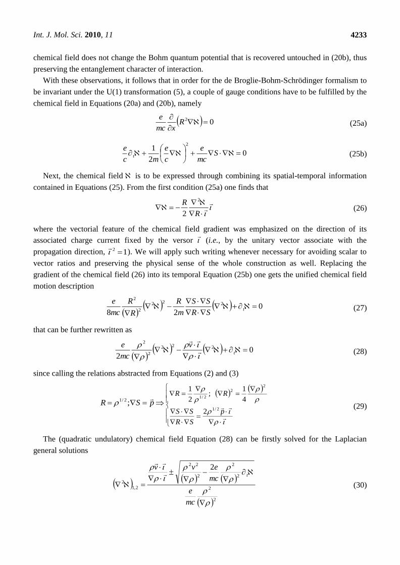
With these observations, it follows that in order for the de Broglie-Bohm-Schrödinger formalism to

be invariant under the U(1) transformation (5), a couple of gauge conditions have to be fulfilled by the

chemical field in Equations (20a) and (20b), namely

02

R

xmc

e (25a)

02

12

S

mc

e

c

e

mc

et (25b)

Next, the chemical field is to be expressed through combining its spatial-temporal information

contained in Equations (25). From the first condition (25a) one finds that

R

R 2

2 (26)

where the vectorial feature of the chemical field gradient was emphasized on the direction of its

associated charge current fixed by the versor

(i.e., by the unitary vector associate with the

propagation direction, 12

). We will apply such writing whenever necessary for avoiding scalar to

vector ratios and preserving the physical sense of the whole construction as well. Replacing the

gradient of the chemical field (26) into its temporal Equation (25b) one gets the unified chemical field

motion description

0

28

222

2

2

t

SR

SS

m

R

R

R

mc

e (27)

that can be further rewritten as

0

2

222

2

2

t

v

mc

e

(28)

since calling the relations abstracted from Equations (2) and (3)

pSR

;2/1

p

SR

SS

RR

2/1

22

2/1

2

4

1;

2

1

(29)

The (quadratic undulatory) chemical field Equation (28) can be firstly solved for the Laplacian

general solutions

2

2

2

2

2

22

2,1

2

2

mc

e

mc

evvt

(30)

Int. J. Mol. Sci. 2010, 11

4234

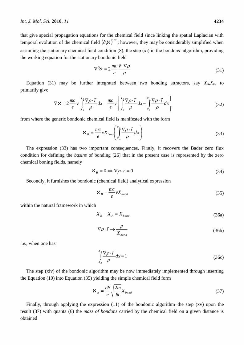
that give special propagation equations for the chemical field since linking the spatial Laplacian with

temporal evolution of the chemical field 2/1 t ; however, they may be considerably simplified when

assuming the stationary chemical field condition (8), the step (xi) in the bondons‘ algorithm, providing

the working equation for the stationary bondonic field

v

e

mc

22 (31)

Equation (31) may be further integrated between two bonding attractors, say XA,XB, to

primarily give

A

B

B

A

B

A

X

X

X

X

X

X

dxdxve

mcdxv

e

mc

2 (32)

from where the generic bondonic chemical field is manifested with the form

B

A

X

X

bondB dxvXe

mc

(33)

The expression (33) has two important consequences. Firstly, it recovers the Bader zero flux

condition for defining the basins of bonding [26] that in the present case is represented by the zero

chemical boning fields, namely

0B 0

(34)

Secondly, it furnishes the bondonic (chemical field) analytical expression

bondB vXe

mc (35)

within the natural framework in which

bondAB XXX (36a)

bondX

(36b)

i.e., when one has

1

B

A

X

X

dx

(36c)

The step (xiv) of the bondonic algorithm may be now immediately implemented through inserting

the Equation (10) into Equation (35) yielding the simple chemical field form

bondB Xt

m

e

c

2 (37)

Finally, through applying the expression (11) of the bondonic algorithm–the step (xv) upon the

result (37) with quanta (6) the mass of bondons carried by the chemical field on a given distance is

obtained

Int. J. Mol. Sci. 2010, 11

4235

2

1

2bond

BX

tm

(38)

Note that the bondons‘ mass (38) directly depends on the time the chemical information ―travels‖

from one bonding attractor to the other involved in bonding, while fast decreasing as the bonding

distance increases. This phenomenological behavior has to be in the sequel cross-checked by

considering the generalized relativistic version of electronic motion by means of the Dirac equation,

Further quantitative consideration will be discussed afterwards.

3.2. Relativistic Bondons

In treating the quantum relativistic electronic behavior, the consecrated starting point stays the

Dirac equation for the scalar real valued potential w that can be seen as a general function of xtc

,

dependency [49]

0

23

1

0ˆˆˆ

wβmcβαcii

k

kkt (39)

with the spatial coordinate derivative notation kk x / and the special operators assuming the

Dirac 4D representation

0ˆ

ˆ0ˆ

k

k

k

,

1̂0

01̂̂ (40a)

in terms of bi-dimensional Pauli and unitary matrices

01

10ˆ

1 ,

0

0ˆ

2i

i ,

10

01ˆ

3 ,

10

01ˆ1̂ 0 (40b)

Written within the de Broglie-Bohm framework, the spinor solution of Equation (39) looks like

sxtSi

sxtSi

xtRxtR

,exp

,exp

,2

1,

2

10

,

2

1s (41)

that from the beginning satisfies the necessary electronic density condition

RR*

0

*

0

(42)

Going on, aiming for the separation of the Dirac Equation (39) into its real/imaginary spinorial

contributions, one firstly calculates the terms

S

iRR ttt

2

1

2

10 (43a)

Int. J. Mol. Sci. 2010, 11

4236

S

iRR kkk

2

1

2

10 (43b)

3

1

3

1

0

3

1 0ˆ

ˆ0

2

1

0ˆ

ˆ0

2

1ˆ

k k

k

k

k k

k

k

k

kk Si

RRα

k kk

k kk

k kk

k kk

S

SiR

R

R

ˆ

ˆ

2

1

ˆ

ˆ

2

1

(43c)

R

mcR

mcmcβ

21̂0

01̂

2

ˆ22

0

2

(43d)

R

wwβ

2

ˆ0

(43e)

to be then combined in (39) producing the actual de Broglie-Bohm-Dirac spinorial Equation

RwmcSRcRci

RwmcSRcRci

SRRi

SRRi

k kkk kk

k kkk kk

tt

tt

2

2

ˆˆ

ˆˆ

(44)

When equating the imaginary parts of (44) one yields the system

0ˆ

0ˆ

RRc

RcR

tk kk

k kkt

(45)

that has non-trivial spinorial solutions only by canceling the associate determinant, i.e., by forming the

Equation

222ˆ

k kkt RcR (46)

of which the minus sign of the squared root corresponds with the electronic conservation charge, while

the positive sign is specific to the relativistic treatment of the positron motion. For proofing this, the

specific relationship for the electronic charge conservation (4) may be unfolded by adapting it to the

present Bohmian spinorial case by the chain equivalences

jt

0

k kkt jR2

k kkt αcRR 0

*

0ˆ2

sS

i

sSi

k

k

k

sSi

sSi

kt

e

eeeRRc

RR

0ˆ

ˆ0

22 *

Int. J. Mol. Sci. 2010, 11

4237

k kkt R

cRR 2

1

2

1

2 )(ˆ2

2

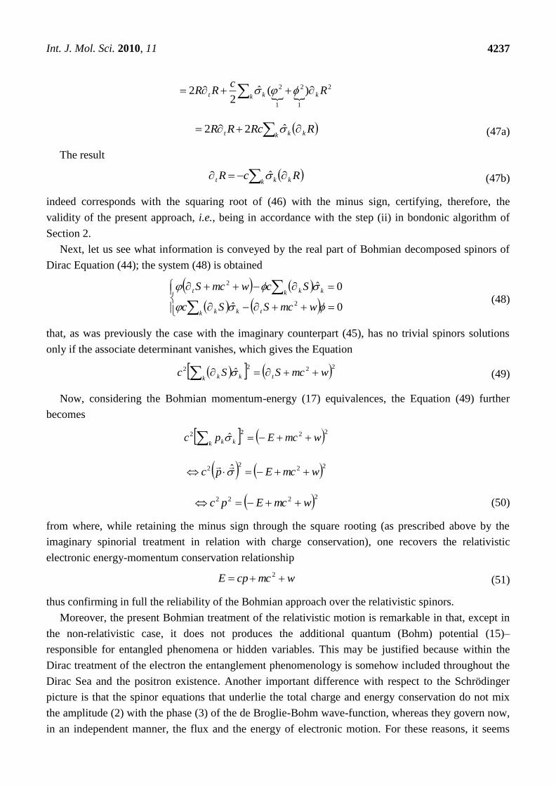
k kkt RRcRR ̂22 (47a)

The result

k kkt RcR ̂ (47b)

indeed corresponds with the squaring root of (46) with the minus sign, certifying, therefore, the

validity of the present approach, i.e., being in accordance with the step (ii) in bondonic algorithm of

Section 2.

Next, let us see what information is conveyed by the real part of Bohmian decomposed spinors of

Dirac Equation (44); the system (48) is obtained

0ˆ

0ˆ

2

2

wmcSSc

ScwmcS

tk kk

k kkt

(48)

that, as was previously the case with the imaginary counterpart (45), has no trivial spinors solutions

only if the associate determinant vanishes, which gives the Equation

2222 ˆ wmcSSc tk kk (49)

Now, considering the Bohmian momentum-energy (17) equivalences, the Equation (49) further

becomes

2222 ˆ wmcEpck kk

222

2 ˆ wmcEpc

2222 wmcEpc (50)

from where, while retaining the minus sign through the square rooting (as prescribed above by the

imaginary spinorial treatment in relation with charge conservation), one recovers the relativistic

electronic energy-momentum conservation relationship

wmccpE 2 (51)

thus confirming in full the reliability of the Bohmian approach over the relativistic spinors.

Moreover, the present Bohmian treatment of the relativistic motion is remarkable in that, except in

the non-relativistic case, it does not produces the additional quantum (Bohm) potential (15)–

responsible for entangled phenomena or hidden variables. This may be justified because within the

Dirac treatment of the electron the entanglement phenomenology is somehow included throughout the

Dirac Sea and the positron existence. Another important difference with respect to the Schrödinger

picture is that the spinor equations that underlie the total charge and energy conservation do not mix

the amplitude (2) with the phase (3) of the de Broglie-Bohm wave-function, whereas they govern now,

in an independent manner, the flux and the energy of electronic motion. For these reasons, it seems

Int. J. Mol. Sci. 2010, 11

4238

that the relativistic Bohmian picture offers the natural environment in which the chemical field and

associate bondons particles may be treated without involving additional physics.

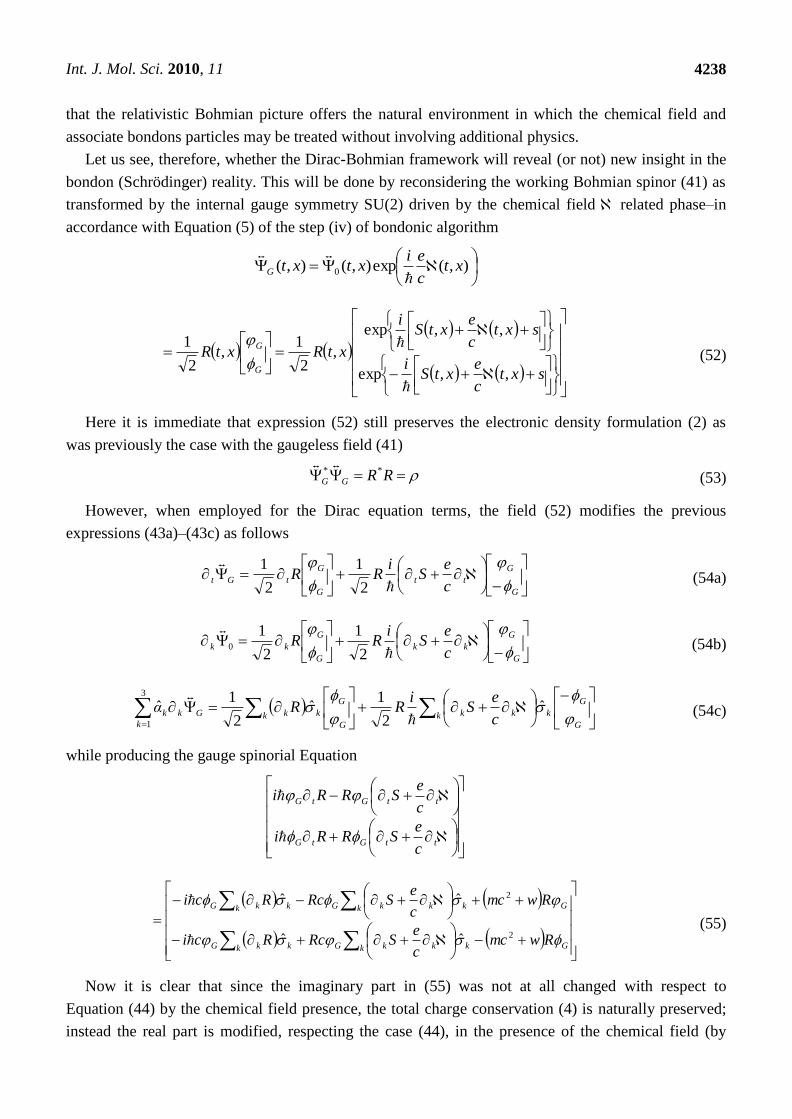
Let us see, therefore, whether the Dirac-Bohmian framework will reveal (or not) new insight in the

bondon (Schrödinger) reality. This will be done by reconsidering the working Bohmian spinor (41) as

transformed by the internal gauge symmetry SU(2) driven by the chemical field related phase–in

accordance with Equation (5) of the step (iv) of bondonic algorithm

),(exp),(),( 0 xt

c

eixtxtG

sxtc

extS

i

sxtc

extS

i

xtRxtRG

G

,,exp

,,exp

,2

1,

2

1

(52)

Here it is immediate that expression (52) still preserves the electronic density formulation (2) as

was previously the case with the gaugeless field (41)

RRGG

**

(53)

However, when employed for the Dirac equation terms, the field (52) modifies the previous

expressions (43a)–(43c) as follows

G

G

tt

G

G

tGtc

eS

iRR

2

1

2

1 (54a)

G

G

kk

G

G

kkc

eS

iRR

2

1

2

10 (54b)

G

G

k kkk

G

G

k kkG

k

kkc

eS

iRRα

ˆ

2

1ˆ

2

1ˆ

3

1

(54c)

while producing the gauge spinorial Equation

ttGtG

ttGtG

c

eSRRi

c

eSRRi

Gk kkkGk kkG

Gk kkkGk kkG

Rwmcc

eSRcRci

Rwmcc

eSRcRci

2

2

ˆˆ

ˆˆ

(55)

Now it is clear that since the imaginary part in (55) was not at all changed with respect to

Equation (44) by the chemical field presence, the total charge conservation (4) is naturally preserved;

instead the real part is modified, respecting the case (44), in the presence of the chemical field (by

Int. J. Mol. Sci. 2010, 11

4239

internal gauge symmetry). Nevertheless, in order that chemical field rotation does not produce

modification in the total energy conservation, it imposes that the gauge spinorial system of the

chemical field must be as

0ˆ

0ˆ

tGk kkG

k kkGtG

c

c

(56)

According to the already custom procedure, for the system (56) having no trivial gauge spinorial

solution, the associated vanishing determinant is necessary, which brings to light the chemical field

Equation

222 ˆ tk kkc (57a)

equivalently rewritten as

22

2 ˆ tc

(57b)

that simply reduces to

222 tc (57c)

through considering the Pauling matrices (40b) unitary feature upon squaring.

At this point, one has to decide upon the sign of the square root of (57c); this was previously

clarified to be minus for electronic and plus for positronic motions. Therefore, the electronic chemical

bond is modeled by the resulting chemical field equation projected on the bonding length direction

tcX bond

1 (58)

The Equation (58) is of undulatory kind with the chemical field solution having the general plane

wave form

tkXie

cbondB exp

(59)

that agrees with both the general definition of the chemical field (6) as well as with the relativistic

―traveling‖ of the bonding information. In fact, this is the paradox of the Dirac approach of the

chemical bond: it aims to deal with electrons in bonding while they have to transmit the chemical

bonding information—as waves—propagating with the light velocity between the bonding attractors.

This is another argument for the need of bondons reality as a specific existence of electrons in

chemical bond is compulsory so that such a paradox can be solved.

Note that within the Dirac approach, the Bader flux condition (9) is no more related to the chemical

field, being included in the total conservation of charge; this is again natural, since in the relativistic

case the chemical field is explicitly propagating with a percentage of light velocity (see the Discussion

in Section 4 below) so that it cannot drive the (stationary) electronic frontiers of bonding.

Further on, when rewriting the chemical field of bonding (59) within the de Broglie and Planck

consecrated corpuscular-undulatory quantifications

Int. J. Mol. Sci. 2010, 11

4240

EtpX

i

e

cXt bondbondB

exp, (60)

it may be further combined with the unitary quanta form (6) in the Equation (11) of the step (xv) in the

bondonic algorithm to produce the phase condition

EtpX

ibond

exp1 (61)

that implies the quantification

nEtpXbond 2 , Nn (62)

By the subsequent employment of the Heisenberg time-energy saturated indeterminacy at the level

of kinetic energy abstracted from the total energy (to focus on the motion of the bondonic plane waves)

tE

(63a)

t

mmTmvp

22 (63b)

the bondon Equation (62) becomes

122

nt

mX bond (64)

that when solved for the bondonic mass yields the expression

2

212

1

2 n

X

tm

bond

B

, n = 0,1,2… (65)

which appears to correct the previous non-relativistic expression (38) with the full quantification.

However, the Schrödinger bondon mass of Equation (38) is recovered from the Dirac bondonic

mass (65) in the ground state, i.e., by setting n = 0. Therefore, the Dirac picture assures the complete

characterization of the chemical bond through revealing the bondonic existence by the internal

chemical field symmetry with the quantification of mass either in ground or in excited states

( 0n , Nn ).

Moreover, as always happens when dealing with the Dirac equation, the positronic bondonic mass

may be immediately derived as well, for the case of the chemical bonding is considered also in the

anti-particle world; it emerges from reloading the square root of the Dirac chemical field

Equation (57c) with a plus sign that will be propagated in all the subsequent considerations, e.g., with

the positronic incoming plane wave replacing the departed electronic one of (59), until delivering the

positronic bondonic mass

2

212

1

2

~ nX

tm

bond

B

, n = 0,1,2… (66)

It nevertheless differs from the electronic bondonic mass (65) only in the excited spectrum, while both

collapse in the non-relativistic bondonic mass (38) for the ground state of the chemical bond.

Int. J. Mol. Sci. 2010, 11

4241

Remarkably, for both the electronic and positronic cases, the associated bondons in the excited

states display heavier mass than those specific to the ground state, a behavior once more confirming

that the bondons encompass all the bonding information, i.e., have the excitation energy converted in

the mass-added-value in full agreement with the mass-energy relativistic custom Einstein

equivalence [64].

4. Discussion

Let us analyze the consequences of the bondon‘s existence, starting from its mass (38) formulation

on the ground state of the chemical bond.

At one extreme, when considering atomic parameters in bonding, i.e., when assuming the bonding

distance of the Bohr radius size SIma ][1052917.0 10

0

the corresponding binding time would be

given as SIsvatt ][1041889.2/ 17

000

while the involved bondonic mass will be half of the

electronic one 2/0m , to assure fast bonding information. Of course, this is not a realistic binding

situation; for that, let us check the hypothetical case in which the electronic 0m mass is combined,

within the bondonic formulation (38), into the bond distance 02/ mtXbond resulting in it

completing the binding phenomenon in the femtosecond time SIbonding st ][10~ 12 for the custom

nanometric distance of bonding SIbond mX ][10~ 9 . Still, when both the femtosecond and nanometer

time-space scale of bonding is assumed in (38), the bondonic mass is provided in the range of

electronic mass SIB kgm ][10~ 31 although not necessarily with the exact value for electron mass nor

having the same value for each bonding case considered. Further insight into the time existence of the

bondons will be reloaded for molecular systems below after discussing related specific properties as

the bondonic velocity and charge.

For enlightenment on the last perspective, let us rewrite the bondonic mass (65) within the spatial-

energetic frame of bonding, i.e., through replacing the time with the associated Heisenberg

energy, bondbonding Et / , thus delivering another working expression for the bondonic mass

2

22 12

2 bondbond

BXE

nm

, n = 0,1,2… (67)

that is more practical than the traditional characterization of bonding types in terms of length and

energy of bonding; it may further assume the numerical ground state ratio form

2

00

][]/[

8603.87

AXmolkcalEm

m

bondbond

Bm

(68)

when the available bonding energy and length are considered (as is the custom for chemical

information) in kcal/mol and Angstrom, respectively. Note that having the bondon‘s mass in terms of

bond energy implies the inclusion of the electronic pairing effect in the bondonic existence, without

the constraint that the bonding pair may accumulate in the internuclear region [69].

Moreover, since the bondonic mass general formulation (65) resulted within the relativistic

treatment of electron, it is considering also the companion velocity of the bondonic mass that is

Int. J. Mol. Sci. 2010, 11

4242

reached in propagating the bonding information between the bonding attractors. As such, when the

Einstein type relationship [70]

hmv

2

2

(69)

is employed for the relativistic bondonic velocity-mass relationship [63,64]

2

2

1c

v

mm

B

B

(70)

and for the frequency of the associate bond wave

bond

B

X

v (71)

it provides the quantified searched bondon to light velocity ratio

22

422

2

12

64

11

1

bondbond

B

XE

ncc

v

, n = 0,1,2…

(72)

or numerically in the bonding ground state as

[%]

][]/[

1027817.31

100

20

2

6

AXmolkcalE

c

v

bondbond

Bv

(73)

Next, dealing with a new matter particle, one will be interested also on its charge, respecting the

benchmarking charge of an electron. To this end, one re-employs the step (xv) of bondonic algorithm,

Equation (11), in the form emphasizing the bondonic charge appearance, namely

0 BB e (74)

Next, when considering for the left-hand side of (74), the form provided by Equation (35), and for the

right-hand side of (74), the fundamental hyperfine value of Equation (6), one gets the working

Equation

Coulomb

meterJouleX

e

vmc bond

B

BB 036.137 (75)

from where the bondonic charge appears immediately, once the associate expressions for mass and

velocity are considered from Equations (67) and (72), respectively, yielding the quantified form

422

222

12

641

1

036.137

4

nc

XE

ce

bondbond

B

, n = 0,1,2…

(76)

Int. J. Mol. Sci. 2010, 11

4243

However, even for the ground state, and more so for the excited states, one may see that when forming

the practical ratio respecting the unitary electric charge from (76), it actually approaches a referential

value, namely

4

121027817.3

][]/[

1

4

46

20

2

n

AXmolkcalEe

e

bondbond

Be

(77)

for, in principle, any common energy and length of chemical bonding. On the other side, for the

bondons to have different masses and velocities (kinetic energy) as associated with specific bonding

energy but an invariant (universal) charge seems a bit paradoxical. Moreover, it appears that with

Equation (77) the predicted charge of a bonding, even in small molecules such as H2, considerably

surpasses the available charge in the system, although this may be eventually explained by the

continuous matter-antimatter balance in the Dirac Sea to which the present approach belongs.

However, to circumvent such problems, one may further use the result (77) and map it into the Poisson

type charge field Equation

eeB 4 42V (78)

from where the bondonic charge may be reshaped by appropriate dimensional scaling in terms of the

bounding parameters (Ebond and Xbond) successively as

0

2

4

1

4

1~

bondbond

XXXB

XEVe

bond (79)

Now, Equation (79) may be employed towards the working ratio between the bondonic and electronic

charges in the ground state of bonding

3

0

1027817.3

][]/[

32

1~

AXmolkcalE

e

e bondbond

Be

(80)

With Equation (80) the situation is reversed compared with the previous paradoxical situation, in

the sense that now, for most chemical bonds (of Table 1, for instance), the resulted bondonic charge is

small enough to be not yet observed or considered as belonging to the bonding wave spreading among

the binding electrons.

Instead, aiming to explore the specific information of bonding reflected by the bondonic mass and

velocity, the associated ratios of Equations (68) and (73) for some typical chemical bonds [71,72] are

computed in Table 1. They may be eventually accompanied by the predicted life-time of corresponding

bondons, obtained from the bondonic mass and velocity working expressions (68) and (73),

respectively, throughout the basic time-energy Heisenberg relationship—here restrained at the level of

kinetic energy only for the bondonic particle; this way one yields the successive analytical forms

SI

vmvmvmBBB

B scmcmvmT

t ][100257618.0102

10

22 15

22

4

2

0

22

0

2

(81)

Int. J. Mol. Sci. 2010, 11

4244

and the specific values for various bonding types that are displayed in Table 1. Note that defining the

bondonic life-time by Equation (81) is the most adequate, since it involves the basic bondonic

(particle!) information, mass and velocity; instead, when directly evaluating the bondonic

life-time by only the bonding energy one deals with the working formula

SI

bondbond

bond smolkcalEE

t ][10]/[

51787.1 14

(82)

that usually produces at least one order lower values than those reported in Table 1 upon employing

the more complex Equation (81). This is nevertheless reasonable, because in the last case no particle

information was considered, so that the Equation (82) gives the time of the associate wave

representation of bonding; this departs by the case when the time is computed by Equation (81) where

the information of bonding is contained within the particle (bondonic) mass and velocity, thus

predicting longer life-times, and consequently a more susceptible timescale in allowing the bondonic

observation. Therefore, as far as the chemical bonding is modeled by associate bondonic particle, the

specific time of Equation (81) rather than that of Equation (82) should be considered.

While analyzing the values in Table 1, it is generally observed that as the bondonic mass is large as

its velocity and the electric charge lower in their ratios, respecting the light velocity and electronic

benchmark charge, respectively, however with some irregularities that allows further discrimination in

the sub-bonding types. Yet, the life-time tendency records further irregularities, due to its complex and

reversed bondonic mass-velocity dependency of Equation (81), and will be given a special role in

bondonic observation—see the Table 2 discussion below. Nevertheless, in all cases, the bondonic

velocity is a considerable (non-negligible) percent of the photonic velocity, confirming therefore its

combined quantum-relativistic nature. This explains why the bondonic reality appears even in the

non-relativistic case of the Schrödinger equation when augmented with Bohmian entangled motion

through the hidden quantum interaction.

Going now to particular cases of chemical bonding in Table 1, the hydrogen molecule maintains its

special behavior through providing the bondonic mass as slightly more than double of the only two

electrons contained in the whole system. This is not a paradox, but a confirmation of the fact the

bondonic reality is not just the sum or partition of the available valence atomic electrons in molecular

bonds, but a distinct (although related) existence that fully involves the undulatory nature of the

electronic and nuclear motions in producing the chemical field. Remember the chemical field was

associated either in Schrödinger as well in Dirac pictures with the internal rotations of the (Bohmian)

wave function or spinors, being thus merely a phase property—thus inherently of undulatory nature. It

is therefore natural that the risen bondons in bonding preserve the wave nature of the chemical field

traveling the bond length distance with a significant percent of light.

Moreover, the bondonic mass value may determine the kind of chemical bond created, in this line

the H2 being the most covalent binding considered in Table 1 since it is most closely situated to the

electronic pairing at the mass level. The excess in H2 bond mass with respect to the two electrons in

isolated H atoms comes from the nuclear motion energy converted (relativistic) and added to the two-

sided electronic masses, while the heavier resulted mass of the bondon is responsible for the

stabilization of the formed molecule respecting the separated atoms. The H2 bondon seems to be also

among the less circulated ones (along the bondon of the F2 molecule) in bonding traveled information

Int. J. Mol. Sci. 2010, 11

4245

due to the low velocity and charge record—offering therefore another criterion of covalency, i.e.,

associated with better localization of the bonding space.

Table 1. Ratios for the bondon-to-electronic mass and charge and for the bondon-to-light

velocity, along the associated bondonic life-time for typical chemical bonds in terms of

their basic characteristics such as the bond length and energy [71,72] through employing

the basic formulas (68), (73), (80) and (81) for the ground states, respectively.

Bond Type bondX

(Å)

bondE

(kcal/mol) 0m

mBm [%]

c

vB

v ]10[ 3

e

eBe ]10[ 15Bt

(seconds)

H–H 0.60 104.2 2.34219 3.451 0.3435 9.236

C–C 1.54 81.2 0.45624 6.890 0.687 11.894

C–C (in diamond) 1.54 170.9 0.21678 14.385 1.446 5.743

C=C 1.34 147 0.33286 10.816 1.082 6.616

CC 1.20 194 0.31451 12.753 1.279 5.037

NN 1.10 225 0.32272 13.544 1.36 4.352

O=O 1.10 118.4 0.61327 7.175 0.716 8.160

F–F 1.28 37.6 1.42621 2.657 0.264 25.582

Cl–Cl 1.98 58 0.3864 6.330 0.631 16.639

I–I 2.66 36.1 0.3440 5.296 0.528 26.701

C–H 1.09 99.2 0.7455 5.961 0.594 9.724

N–H 1.02 93.4 0.9042 5.254 0.523 10.32

O–H 0.96 110.6 0.8620 5.854 0.583 8.721

C–O 1.42 82 0.5314 6.418 0.64 11.771

C=O (in CH2O) 1.21 166 0.3615 11.026 1.104 5.862

C=O (in O=C=O) 1.15 191.6 0.3467 12.081 1.211 5.091

C–Cl 1.76 78 0.3636 7.560 0.754 12.394

C–Br 1.91 68 0.3542 7.155 0.714 14.208

C–I 2.10 51 0.3906 5.905 0.588 18.9131

The same happens with the C–C bonding, which is predicted to be more covalent for its simple

(single) bondon that moves with the smallest velocity (v

<<) or fraction of the light velocity from all

C–C types of bonding; in this case also the bondonic highest mass ( m >>), smallest charge (

e <<),

and highest (observed) life-time ( Bt >>) criteria seem to work well. Other bonds with high covalent

character, according with the bondonic velocity criterion only, are present in NN and the C=O

bonding types and less in the O=O and C–O ones. Instead, one may establish the criteria for multiple

(double and triple) bonds as having the series of current bondonic properties as:

},,,{ Bevm

t .

However, the diamond C–C bondon, although with the smallest recorded mass ( m <<), is

characterized by the highest velocity ( v >) and charge ( e

>) in the CC series (and also among all

cases of Table 1). This is an indication that the bond is very much delocalized, thus recognizing the

solid state or metallic crystallized structure for this kind of bond in which the electronic pairings (the

bondons) are distributed over all atomic centers in the unit cell. It is, therefore, a special case of

bonding that widely informs us on the existence of conduction bands in a solid; therefore the metallic

Int. J. Mol. Sci. 2010, 11

4246

character generally associated with the bondonic series of properties },,,{ Bevm

t , thus

having similar trends with the corresponding properties of multiple bonds, with the only particularity

in the lower mass behavior displayed—due to the higher delocalization behavior for the

associate bondons.

Very interestingly, the series of C–H, N–H, and O–H bonds behave similarly among them since

displaying a shrink and medium range of mass (moderate high), velocity, charge and life-time

(moderate high) variations for their bondons, }~~,~,,~{ Bevm

t ; this may explain why these

bonds are the most preferred ones in DNA and genomic construction of proteins, being however

situated towards the ionic character of chemical bond by the lower bondonic velocities computed; they

have also the most close bondonic mass to unity; this feature being due to the manifested polarizability

and inter-molecular effects that allows the 3D proteomic and specific interactions taking place.

Instead, along the series of halogen molecules F2, Cl2, and I2, only the observed life-time of

bondons show high and somehow similar values, while from the point of view of velocity and charge

realms only the last two bonding types display compatible properties, both with drastic difference for

their bondonic mass respecting the F–F bond—probably due the most negative character of the

fluorine atoms. Nevertheless, judging upon the higher life-time with respect to the other types of

bonding, the classification may be decided in the favor of covalent behavior. At this point, one notes

traces of covalent bonding nature also in the case of the rest of halogen-carbon binding (C–Cl, C–Br,

and C–I in Table 1) from the bondonic life-time perspective, while displaying also the ionic

manifestation through the velocity and charge criteria ~}~,{ ev and even a bit of metal character by

the aid of small bondonic mass (m

<). All these mixed features may be because of the joint existence

of both inner electronic shells that participate by electronic induction in bonding as well as

electronegativity difference potential.

Remarkably, the present results are in accordance with the recent signalized new binding class

between the electronic pairs, somehow different from the ionic and covalent traditional ones in the

sense that it is seen as a kind of resonance, as it appears in the molecular systems like F2, O2, N2 (with

impact in environmental chemistry) or in polar compounds like C–F (specific to ecotoxicology) or in

the reactions that imply a competition between the exchange in the hydrogen or halogen (e.g., HF).

The valence explanation relied on the possibility of higher orders of orbitals‘ existing when additional

shells of atomic orbitals are involved such as <f> orbitals reaching this way the charge-shift bonding

concept [73]; the present bondonic treatment of chemical bonds overcomes the charge shift paradoxes

by the relativistic nature of the bondon particles of bonding that have as inherent nature the time-space

or the energy-space spanning towards electronic pairing stabilization between centers of bonding or

atomic adducts in molecules.

However, we can also made predictions regarding the values of bonding energy and length required

for a bondon to acquire either the unity of electronic charge or its mass (with the consequence in its

velocity fraction from the light velocity) on the ground state, by setting Equations (68) and (80) to

unity, respectively. These predictions are summarized in Table 2.

From Table 2, one note is that the situation of the bondon having the same charge as the electron is

quite improbable, at least for the common chemical bonds, since in such a case it will feature almost

the light velocity (and almost no mass–that is, however, continuously decreasing as the bonding energy

Int. J. Mol. Sci. 2010, 11

4247

decreases and the bonding length increases). This is natural since a longer distance has to be spanned

by lower binding energy yet carrying the same unit charge of electron while it is transmitted with the

same relativistic velocity! Such behavior may be regarded as the present zitterbewegung (trembling in

motion) phenomena, here at the bondonic level. However one records the systematic increasing of

bondonic life-time towards being observable in the femtosecond regime for increasing bond length and

decreasing the bonding energy–under the condition the chemical bonding itself still exists for certain

{ bondX , bondE } combinations.

Table 2. Predicted basic values for bonding energy and length, along the associated

bondonic life-time and velocity fraction from the light velocity for a system featuring unity

ratios of bondonic mass and charge, respecting the electron values, through employing the

basic formulas (81), (73), (68), and (80), respectively.

bondX

][0

A bondE

]/[ molkcal

]10[ 15Bt

(seconds)

[%]c

vBv

0m

mBm

e

eBe

1 87.86 10.966 4.84691 1 0.4827 × 10 –3

1 182019 53.376 99.9951 4.82699 × 10 –4

1

10 18201.9 533.76 99.9951 4.82699 × 10 –5

1

100 1820.19 5337.56 99.9951 4.82699 × 10 –6

1

On the other side, the situation in which the bondon will weigh as much as one electron is a current

one (see the Table 1); nevertheless, it is accompanied by quite reasonable chemical bonding length and

energy information that it can carried at a low fraction of the light velocity, however with very low

charge as well. Nevertheless, the discovered bonding energy-length relationship from Table 2, based

on Equation (80), namely

182019][]/[0

AXmolkcalE bondbond (83)

should be used in setting appropriate experimental conditions in which the bondon particle B may be

observed as carrying the unit electronic charge yet with almost zero mass. In this way, the bondon is

affirmed as a special particle of Nature, that when behaving like an electron in charge it is behaving

like a photon in velocity and like neutrino in mass, while having an observable (at least as

femtosecond) lifetime for nanosystems having chemical bonding in the range of hundred of Angstroms

and thousands of kcal/mol! Such a peculiar nature of a bondon as the quantum particle of chemical

bonding, the central theme of Chemistry, is not as surprising when noting that Chemistry seems to

need both a particle view (such as offered by relativity) and a wave view (such as quantum mechanics

offers), although nowadays these two physics theories are not yet fully compatible with each other, or

even each fully coherent internally. Maybe the concept of ‗bondons‘ will help to improve the situation

for all concerned by its further conceptual applications.

Finally, just to give a conceptual glimpse of how the present bondonic approach may be employed,

the scattering phenomena are considered within its Raman realization, viewed as a sort of generalized

Compton scattering process, i.e., extracting the structural information from various systems (atoms,

molecules, crystals, etc.) by modeling the inelastic interaction between an incident IR photon and a

quantum system (here the bondons of chemical bonds in molecules), leaving a scattered wave with

Int. J. Mol. Sci. 2010, 11

4248

different frequency and the resulting system in its final state [74]. Quantitatively, one firstly considers

the interaction Hamiltonian as being composed by two parts,

j

jjB

B

B trApm

eH ),()1(

(84)

j

j

B

B trAm

eH ),(

2

2

)2( 2

(85)

accounting for the linear and quadratic dependence of the light field potential vector ),( trAj

acting on

the bondons ―j‖, carrying the kinetic moment BBjB

vmp , charge Be and mass

Bm .

Then, noting that, while considering the quantified incident ( 00 ,q

) and scattered ( ,q

) light

beams, the interactions driven by H(1)

and H(2)

model the changing in one- and two- occupation

numbers of photonic trains, respectively. In this context, the transition probability between the initial

iB and final fB bondonic states writes by squaring the sum of all scattering quantum probabilities

that include absorption (A, with nA number of photons) and emission (E, with nE number of photons) of

scattered light on bondons, see Figure 1.

Figure 1. The Feynman diagrammatical sum of interactions entering the Raman effect by

connecting the single and double photonic particles‘ events in absorption (incident wave

light 00 ,q

) and emission (scattered wave light ,q

) induced by the quantum first H(1)

and

second H(2)

order interaction Hamiltonians of Equations (84) and (85) through the

initial iB , final fB , and virtual vB bondonic states. The first term accounts for

absorption (A)-emission (E) at once, the second term sums over the virtual states

connecting the absorption followed by emission, while the third terms sums over virtual

states connecting the absorption following the emission events.

Analytically, one has the initial-to-final total transition probability [75]dependence here given as

ddhEhEdfi BBfifi

2

0

22 1

~

Int. J. Mol. Sci. 2010, 11

4249

innHnnf EAEA ;,1,1;1 )2(

v viB BB

iEAEAvvEAEAf

hEE

BnnHnnBBnnHnnB

0

)1()1( ;,,1;;,11,1;

2

)1()1( ;,1,;;1,1,1;

vvi

B BB

iEAEAvvEAEAf

hEE

BnnHnnBBnnHnnB

ddhEhEfi BB

2

0 (86)

At this point, the conceptual challenge appears to explore the existence of the Raman process itself

from the bondonic description of the chemical bond that turns the incoming IR photon into the

(induced, stimulated, or spontaneous) structural frequencies

h

EEvi BB

iv

(87)

As such, the problem may be reshaped in expressing the virtual state energy vB

E in terms of bonding

energy associated with the initial state

bondBEE

i (88)

that can be eventually measured or computationally predicted by other means. However, this further

implies the necessity of expressing the incident IR photon with the aid of bondonic quantification; to

this end the Einstein relation (69) is appropriately reloaded in the form

2

2

222

124

1

2

v

bondbond

BBB

ivn

XE

vvmh

(89)

where the bondonic mass (67) was firstly implemented. Next, in terms of representing the turn of the

incoming IR photon into the structural wave-frequency related with the bonding energy of initial state,

see Equation (88); the time of wave-bond (82) is here considered to further transform Equation (89) to

the yield

2

2

22

2

222

124

112

4

1

v

bond

B

bondv

bondbond

bondbondB

ivn

v

vEn

XE

tEvh (90)

where also the corresponding wave-bond velocity was introduced

bondbond

bond

bondbond XE

t

Xv

1 (91)

Int. J. Mol. Sci. 2010, 11

4250

It is worth noting that, as previously was the case with the dichotomy between bonding and bondonic

times, sees Equations (81) vs. (82), respectively, the bonding velocity of Equation (91) clearly differs

by the bondonic velocity of Equation (72) since the actual working expression

[%]1019758.2][]/[ 30

AXmolkcalE

c

vbondbond

bond (92)

provides considerably lower values than those listed in Table 1–again, due to missing the inclusion of

the particle mass‘ information, unlike is the case for the bondonic velocity.

Returning to the bondonic description of the Raman scattering, one replaces the virtual photonic

frequency of Equation (90) together with Equation (88) back in the Bohr-type Equation (87) to yield

the searched quantified form of virtual bondonic energies in Equation (86) and Figure 1, analytically

2

2

2

124

11

v

bond

B

bondBn

v

vEE

v

4

22

22

2

2

2

1264

12161

v

bondbond

v

bond

nc

XE

nE

(93)

or numerically

4

20

26

22

12][]/[10305048.0

12161

vbondbond

v

bondB

nAXmolkcalE

nEE

v

, nv = 0,1,2… (94)

Remarkably, the bondonic quantification (94) of the virtual states of Raman scattering varies from

negative to positive energies as one moves from the ground state to more and more excited states of

initial bonding state approached by the incident IR towards virtual ones, as may be easily verified by

considering particular bonding data of Table 1. In this way, more space is given for future

considerations upon the inverse or stimulated Raman processes, proving therefore the direct

involvement of the bondonic reality in combined scattering of light on chemical structures.

Overall, the bondonic characterization of the chemical bond is fully justified by quantum and

relativistic considerations, to be advanced as a useful tool in characterizing chemical reactivity, times

of reactions, i.e., when tunneling or entangled effects may be rationalized in an analytical manner.

Note that further correction of this bondonic model may be realized when the present point-like

approximation of nuclear systems is abolished and replaced by the bare-nuclear assumption in which

additional dependence on the bonding distance is involved. This is left for future communications.

5. Conclusion

The chemical bond, perhaps the greatest challenge in theoretical chemistry, has generated many

inspiring theses over the years, although none definitive. Few of the most preeminent regard the

orbitalic based explanation of electronic pairing, in valence shells of atoms and molecules, rooted in

Int. J. Mol. Sci. 2010, 11

4251

the hybridization concept [8] then extended to the valence-shell electron-pair repulsion (VSEPR) [76].

Alternatively, when electronic density is considered, the atoms-in-molecule paradigms were

formulated through the geometrical partition of forces by Berlin [69], or in terms of core, bonding, and

lone-pair lodges by Daudel [77], or by the zero local flux in the gradient field of the density by

Bader [26], until the most recent employment of the chemical action functional in bonding [78,79].

Yet, all these approaches do not depart significantly from the undulatory nature of electronic motion

in bonding, either by direct wave-function consideration or through its probability information in

electronic density manifestation (for that is still considered as a condensed—observable version—of

the undulatory manifestation of electron).

In other words, while passing from the Lewis point-like ansatz to the undulatory modeling of

electrons in bonding, the reverse passage was still missing in an analytical formulation. Only recently

the first attempt was formulated, based on the broken-symmetry approach of the Schrödinger

Lagrangean with the electronegativity-chemical hardness parabolic energy dependency, showing that a

systematical quest for the creation of particles from the chemical bonding fields is possible [80].

Following this line, the present work makes a step forward and considers the gauge transformation

of the electronic wave-function and spinor over the de Broglie-Bohm augmented non-relativistic and

relativistic quantum pictures of the Schrödinger and Dirac electronic (chemical) fields, respectively.

As a consequence, the reality of the chemical field in bonding was proved in either framework, while

providing the corresponding bondonic particle with the associate mass and velocity in a full

quantization form, see Equations (67) and (72). In fact, the Dirac bondon (65) was found to be a

natural generalization of the Schrödinger one (38), while supplementing it with its anti-bondon particle

(66) for the positron existence in the Dirac Sea.

The bondon is the quantum particle corresponding to the superimposed electronic pairing effects or

distribution in chemical bond; accordingly, through the values of its mass and velocity it may be

possible to indicate the type of bonding (in particular) and the characterization of electronic behavior

in bonding (in general).

However, one of the most important consequences of bondonic existence is that the chemical

bonding may be described in a more complex manner than relaying only on the electrons, but

eventually employing the fermionic (electronic)-bosonic (bondonic) mixture: the first preeminent

application is currently on progress, that is, exploring the effect that the Bose-Einstein condensation

has on chemical bonding modeling [81,82]. Yet, such possibility arises due to the fact that whether the

Pauli principle is an independent axiom of quantum mechanics or whether it depends on other quantum

description of matter is still under question [83], as is the actual case of involving hidden variables and

the entanglement or non-localization phenomenology that may be eventually mapped onto the

delocalization and fractional charge provided by quantum chemistry over and on atomic centers of a

molecular complex/chemical bond, respectively.

As an illustration of the bondonic concept and of its properties such as the mass, velocity, charge,

and life-time, the fundamental Raman scattering process was described by analytically deriving the

involved virtual energy states of scattering sample (chemical bond) in terms of the bondonic properties

above—proving its necessary existence and, consequently, of the associate Raman effect itself, while

leaving space for further applied analysis based on spectroscopic data on hand.

Int. J. Mol. Sci. 2010, 11

4252

On the other side, the mass, velocity, charge, and life-time properties of the bondons were

employed for analyzing some typical chemical bonds (see Table 1), this way revealing a sort of fuzzy

classification of chemical bonding types in terms of the bondonic-to-electronic mass and charge ratios

m and e , and of the bondonic-to-light velocity percent ratio v , along the bondonic observable life-

time, Bt respectively–here summarized in Table 3.

Table 3. Phenomenological classification of the chemical bonding types by bondonic

(mass, velocity, charge and life-time) properties abstracted from Table 1; the used symbols

are: > and >> for ‗high‘ and ‗very high‘ values; < and << for ‗low‘ and ‗very low‘ values;

~ and ~> for ‗moderate‘ and ‗moderate high and almost equal‘ values in their class of

bonding.

Property

Chemical bond m

v e Bt

Covalence >> << << >>

Multiple bonds < > > <

Metallic << > > <

Ionic ~> ~ ~ ~>

These rules are expected to be further refined through considering the new paradigms of special

relativity in computing the bondons‘ velocities, especially within the modern algebraic chemistry [84].

Yet, since the bondonic masses of chemical bonding ground states seem untouched by the Dirac

relativistic considerations over the Schrödinger picture, it is expected that their analytical values may

make a difference among the various types of compounds, while their experimental detection is hoped

to be some day completed.

Acknowledgements

The author kindly thanks Hagen Kleinert and Axel Pelster for their hospitality at Free University of

Berlin on many occasions and for the summer of 2010 where important discussions on fundamental

quantum ideas were undertaken in completing this work, as well for continuous friendship through the

last decade. Both anonymous referees are kindly thanked for stimulating the revised version of the

present work, especially regarding the inclusion of the quantum-relativistic charge (zitterbewegung)

discussion and the Raman scattering description by the bondonic particles, respectively. This work was

supported by CNCSIS-UEFISCSU, project number PN II-RU TE16/2010.

References

1. Thomson, J.J. On the structure of the molecule and chemical combination. Philos. Mag. 1921, 41,

510–538.

2. Hückel, E. Quantentheoretische beiträge zum benzolproblem. Z. Physik 1931, 70, 204–286.

3. Doering, W.V; Detert, F. Cycloheptatrienylium oxide. J. Am. Chem. Soc. 1951, 73, 876–877.

4. Lewis, G.N. The atom and the molecule. J. Am. Chem. Soc. 1916, 38, 762–785.

Int. J. Mol. Sci. 2010, 11

4253

5. Langmuir, I. The arrangement of electrons in atoms and molecules. J. Am. Chem. Soc. 1919, 41,

868–934.

6. Pauling, L. Quantum mechanics and the chemical bond. Phys. Rev. 1931, 37, 1185–1186.

7. Pauling, L. The nature of the chemical bond. I. Application of results obtained from the quantum

mechanics and from a theory of paramagnetic susceptibility to the structure of molecules. J. Am.

Chem. Soc. 1931, 53, 1367–1400.

8. Pauling, L. The nature of the chemical bond II. The one-electron bond and the three-electron

bond. J. Am. Chem. Soc. 1931, 53, 3225–3237.

9. Heitler, W.; London, F. Wechselwirkung neutraler Atome und homöopolare Bindung nach der

Quantenmechanik. Z. Phys. 1927, 44, 455–472.

10. Slater, J.C. The self consistent field and the structure of atoms. Phys. Rev. 1928, 32, 339–348.

11. Slater, J.C. The theory of complex spectra. Phys. Rev. 1929, 34, 1293–1322.

12. Hartree, D.R. The Calculation of Atomic Structures; Wiley & Sons: New York, NY, USA, 1957.

13. Löwdin, P.O. Quantum theory of many-particle systems. I. Physical interpretations by means of

density matrices, natural spin-orbitals, and convergence problems in the method of

configurational interaction. Phys. Rev. 1955, 97, 1474–1489.

14. Löwdin, P.O. Quantum theory of many-particle systems. II. Study of the ordinary Hartree-Fock

approximation. Phys. Rev. 1955, 97, 1474–1489.

15. Löwdin, P.O. Quantum theory of many-particle systems. III. Extension of the Hartree-Fock

scheme to include degenerate systems and correlation effects. Phys. Rev. 1955, 97, 1509–1520.

16. Roothaan, C.C.J. New developments in molecular orbital theory. Rev. Mod. Phys. 1951, 23,

69–89.

17. Pariser, R.; Parr, R. A semi-empirical theory of the electronic spectra and electronic structure of

complex unsaturated molecules. I. J. Chem. Phys. 1953, 21, 466–471.

18. Pariser, R.; Parr, R. A semi‐empirical theory of the electronic spectra and electronic structure of

complex unsaturated molecules. II. J. Chem. Phys. 1953, 21, 767–776.

19. Pople, J.A. Electron interaction in unsaturated hydrocarbons. Trans. Faraday Soc. 1953, 49,

1375–1385.

20. Hohenberg, P.; Kohn, W. Inhomogeneous electron gas. Phys. Rev. 1964, 136, B864–B871.

21. Kohn, W.; Sham, L.J. Self-consistent equations including exchange and correlation effects. Phys.

Rev.1965, 140, A1133–A1138.

22. Pople, J.A.; Binkley, J.S.; Seeger, R. Theoretical models incorporating electron correlation. Int. J.

Quantum Chem. 1976, 10, 1–19.

23. Head-Gordon, M.; Pople, J.A.; Frisch, M.J. Quadratically convergent simultaneous optimization

of wavefunction and geometry. Int. J. Quantum Chem. 1989, 36, 291–303.

24. Putz, M.V. Density functionals of chemical bonding. Int. J. Mol. Sci. 2008, 9, 1050–1095.

25. Putz, M.V. Path integrals for electronic densities, reactivity indices, and localization functions in

quantum systems. Int. J. Mol. Sci. 2009, 10, 4816–4940.

26. Bader, R.F.W. Atoms in Molecules-A Quantum Theory; Oxford University Press: Oxford, UK,

1990.

27. Bader, R.F.W. A bond path: A universal indicator of bonded interactions. J. Phys. Chem. A 1998,

102, 7314–7323.

Int. J. Mol. Sci. 2010, 11

4254

28. Bader, R.F.W. Principle of stationary action and the definition of a proper open system. Phys. Rev.

B 1994, 49, 13348–13356.

29. Mezey, P.G. Shape in Chemistry: An Introduction to Molecular Shape and Topology; VCH

Publishers: New York, NY, USA, 1993.

30. Maggiora, G.M.; Mezey, P.G. A fuzzy-set approach to functional-group comparisons based on an

asymmetric similarity measure. Int. J. Quantum Chem. 1999, 74, 503–514.

31. Szekeres, Z.; Exner, T.; Mezey, P.G. Fuzzy fragment selection strategies, basis set dependence

and HF–DFT comparisons in the applications of the ADMA method of macromolecular quantum

chemistry. Int. J. Quantum Chem. 2005, 104, 847–860.

32. Parr, R.G.; Yang, W. Density Functional Theory of Atoms and Molecules; Oxford University

Press: Oxford, UK, 1989.

33. Putz, M.V. Contributions within Density Functional Theory with Applications in Chemical

Reactivity Theory and Electronegativity. Ph.D. dissertation, West University of Timisoara,

Romania, 2003.

34. Sanderson, R.T. Principles of electronegativity Part I. General nature. J. Chem. Educ. 1988, 65,

112–119.

35. Mortier, W.J.; Genechten, K.v.; Gasteiger, J. Electronegativity equalization: Application and

parametrization. J. Am. Chem. Soc. 1985, 107, 829–835.

36. Parr, R.G.; Donnelly, R.A.; Levy, M.; Palke, W.E. Electronegativity: The density functional

viewpoint. J. Chem. Phys. 1978, 68, 3801–3808.

37. Sen, K.D.; Jørgenson, C.D. Structure and Bonding; Springer: Berlin, Germany, 1987; Volume 66.

38. Pearson, R.G. Hard and Soft Acids and Bases; Dowden, Hutchinson & Ross: Stroudsberg, PA,

USA, 1973.

39. Pearson, R.G. Hard and soft acids and bases—the evolution of a chemical concept. Coord. Chem.

Rev. 1990, 100, 403–425.

40. Putz, M.V.; Russo, N.; Sicilia, E. On the applicability of the HSAB principle through the use of

improved computational schemes for chemical hardness evaluation. J. Comp. Chem. 2004, 25,

994–1003.

41. Chattaraj, P.K.; Lee, H.; Parr, R.G. Principle of maximum hardness. J. Am. Chem. Soc. 1991, 113,

1854–1855.

42. Chattaraj, P.K.; Schleyer, P.v.R. An ab initio study resulting in a greater understanding of the

HSAB principle. J. Am. Chem. Soc. 1994, 116, 1067–1071.

43. Chattaraj, P.K.; Maiti, B. HSAB principle applied to the time evolution of chemical reactions. J.

Am. Chem. Soc. 2003, 125, 2705–2710;

44. Putz, M.V. Maximum hardness index of quantum acid-base bonding. MATCH Commun. Math.

Comput. Chem. 2008, 60, 845–868.

45. Putz, M.V. Systematic formulation for electronegativity and hardness and their atomic scales

within densitiy functional softness theory. Int. J. Quantum Chem. 2006, 106, 361–386.

46. Putz, M.V. Absolute and Chemical Electronegativity and Hardness; Nova Science Publishers:

New York, NY, USA, 2008.

47. Dirac, P.A.M. Quantum mechanics of many-electron systems. Proc. Roy. Soc. (London) 1929,

A123, 714–733.

Int. J. Mol. Sci. 2010, 11

4255

48. Schrödinger, E. An undulatory theory of the mechanics of atoms and molecules. Phys. Rev. 1926,

28, 1049–1070.

49. Dirac, P.A.M. The quantum theory of the electron. Proc. Roy. Soc. (London) 1928, A117,

610–624.

50. Einstein, A.; Podolsky, B.; Rosen, N. Can quantum-mechanical description of physical reality be

considered complete? Phys. Rev. 1935, 47, 777–780.

51. Bohr, N. Can quantum-mechanical description of physical reality be considered complete? Phys.

Rev. 1935, 48, 696–702.

52. Bohm, D. A suggested interpretation of the quantum theory in terms of "hidden" variables. I.

Phys. Rev. 1952, 85, 166–179.

53. Bohm, D. A suggested interpretation of the quantum theory in terms of "hidden" variables. II.

Phys. Rev. 1952, 85, 180–193.

54. de Broglie, L. Ondes et quanta. Compt. Rend. Acad. Sci. (Paris) 1923, 177, 507–510.

55. de Broglie, L. Sur la fréquence propre de l'électron. Compt. Rend. Acad. Sci. (Paris) 1925, 180,

498-500.

56. de Broglie, L.; Vigier, M.J.P. La Physique Quantique Restera-t-elle Indéterministe? Gauthier-

Villars: Paris, France, 1953.

57. Bohm, D.; Vigier, J.P. Model of the causal interpretation of quantum theory in terms of a fluid

with irregular fluctuations. Phys. Rev. 1954, 96, 208–216.

58. Pyykkö, P.; Zhao, L.-B. Search for effective local model potentials for simulation of QED effects

in relativistic calculations. J. Phys. B 2003, 36, 1469–1478.

59. Pyykkö, P. Relativistic theory of atoms and molecules. III. A Bibliography 1993–1999, Lecture

Notes in Chemistry, Springer-Verlag: Berlin, Germany, 2000; Volume 76.

60. Snijders, J.G.; Pyykkö, P. Is the relativistic contraction of bond lengths an orbital contraction

effect? Chem. Phys. Lett. 1980, 75, 5–8.

61. Lohr, L.L., Jr.; Pyykkö, P. Relativistically parameterized extended Hückel theory. Chem. Phys.

Lett. 1979, 62, 333–338.

62. Pyykkö, P. Relativistic quantum chemistry. Adv. Quantum Chem. 1978, 11, 353–409.

63. Einstein, A. On the electrodynamics of moving bodies. Ann. Physik (Leipzig) 1905, 17, 891–921.

64. Einstein, A. Does the inertia of a body depend upon its energy content? Ann. Physik (Leipzig)

1905, 18, 639–641.

65. Whitney, C.K. Closing in on chemical bonds by opening up relativity theory. Int. J. Mol. Sci.

2008, 9, 272–298.

66. Whitney, C.K. Single-electron state filling order across the elements. Int. J. Chem. Model. 2008,

1, 105–135.

67. Whitney, C.K. Visualizing electron populations in atoms. Int. J. Chem. Model. 2009, 1, 245–297.

68. Boeyens, J.C.A. New Theories for Chemistry; Elsevier: New York, NY, USA, 2005.

69. Berlin, T. Binding regions in diatomic molecules. J. Chem. Phys. 1951, 19, 208–213.

70. Einstein, A. On a Heuristic viewpoint concerning the production and transformation of light. Ann.

Physik (Leipzig) 1905, 17, 132–148.

71. Oelke, W.C. Laboratory Physical Chemistry; Van Nostrand Reinhold Company: New York, NY,

USA, 1969.

Int. J. Mol. Sci. 2010, 11

4256

72. Findlay, A. Practical Physical Chemistry; Longmans: London, UK, 1955.

73. Hiberty, P.C.; Megret, C.; Song, L.; Wu, W.; Shaik, S. Barriers of hydrogen abstraction vs

halogen exchange: An experimental manifestation of charge-shift bonding. J. Am. Chem. Soc.

2006, 128, 2836–2843.

74. Freeman, S. Applications of Laser Raman Spectroscopy; John Wiley and Sons: New York, NY,

USA, 1974.

75. Heitler, W. The Quantum Theory of Radiation, 3rd ed.; Cambridge University Press: New York,

NY, USA, 1954.

76. Gillespie, R.J. The electron-pair repulsion model for molecular geometry. J. Chem. Educ. 1970,

47, 18–23.

77. Daudel, R. In Electron and Magnetization Densities in Molecules and Crystals; Becker, P., Ed.;

NATO ASI, Series B-Physics, Plenum Press: New York, NY, USA, 1980; Volume 40.

78. Putz, M.V. Chemical action and chemical bonding. J. Mol. Struct. (THEOCHEM) 2009, 900,

64–70.

79. Putz, M.V. Levels of a unified theory of chemical interaction. Int. J. Chem. Model. 2009, 1,

141–147.

80. Putz, M.V. The chemical bond: Spontaneous symmetry–breaking approach. Symmetr. Cult. Sci.

2008, 19, 249–262.

81. Putz, M.V. Hidden side of chemical bond: The bosonic condensate. In Chemical Bonding; NOVA

Science Publishers: New York, NY, USA, 2011; to be published.

82. Putz, M.V. Conceptual density functional theory: From inhomogeneous electronic gas to Bose-

Einstein condensates. In Chemical Information and Computational Challenges in 21st. A

Celebration of 2011 International Year of Chemistry; Putz, M.V., Ed.; NOVA Science Publishers

Inc.: New York, NY, USA, 2011; to be published.

83. Kaplan, I.G. Is the Pauli exclusive principle an independent quantum mechanical postulate? Int. J.

Quantum Chem. 2002, 89, 268–276.

84. Whitney, C.K. Relativistic dynamics in basic chemistry. Found. Phys. 2007, 37, 788–812.

© 2010 by the author; licensee MDPI, Basel, Switzerland. This article is an open access article

distributed under the terms and conditions of the Creative Commons Attribution license

(http://creativecommons.org/licenses/by/3.0/).