The big M method

LI Xiao-lei

The big M method

• The simplex algorithm requires a starting bfs. We found a starting bfs by using the slack variables as our basic variables.

• If an LP has any ≥ or equality constraints, a starting bfs may not be readily apparent.

• The big M method (or the two-phase simplex method) may be used.

Example 4

• Bevco manufactures an orange-flavored soft drink called Oranj by combining orange soda and orange juice.

Each ounce of orange soda contains 0.5 oz of sugar and 1 mg of vitamin C. each ounce of orange juice contains 0.25 oz of sugar and 3 mg of vitamin C.

It costs Bevco 2¢ to produce an ounce of orange soda and 3¢ to produce an ounce of orange juice.

Example 4

• Bevco's marketing department has decided that each 10-oz bottle of Oranj must contain at least 20 mg of vitamin C and at most 4 oz of sugar.

Use LP to determine how Bevco can meet the marketing department's requirements at minimum cost.

Example 4

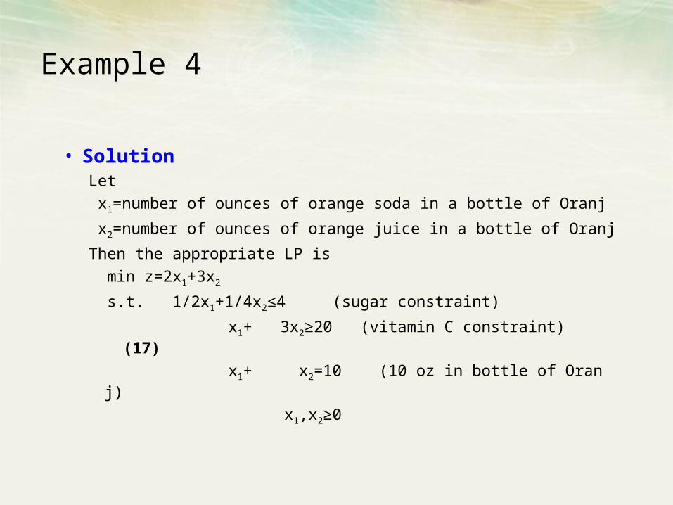
• SolutionLet

x1=number of ounces of orange soda in a bottle of Oranj

x2=number of ounces of orange juice in a bottle of Oranj

Then the appropriate LP is

min z=2x1+3x2

s.t. 1/2x1+1/4x2≤4 (sugar constraint)

x1+ 3x2≥20 (vitamin C constraint) (17)

x1+ x2=10 (10 oz in bottle of Oranj)

x1,x2≥0

Example 4

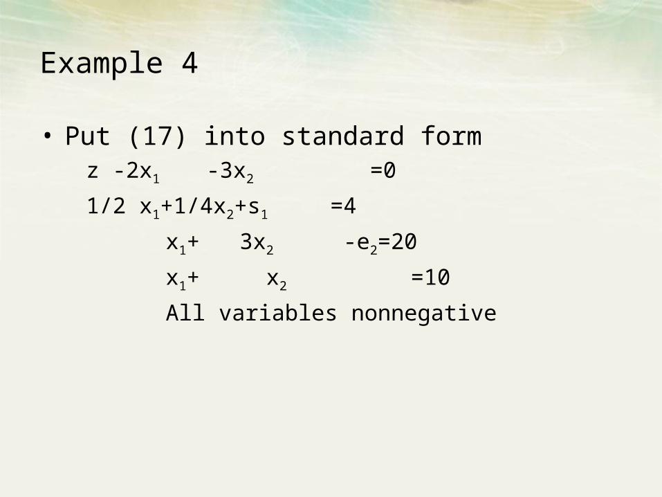
• Put (17) into standard form z -2x1 -3x2 =0

1/2 x1+1/4x2+s1 =4

x1+ 3x2 -e2=20

x1+ x2 =10

All variables nonnegative

Example 4

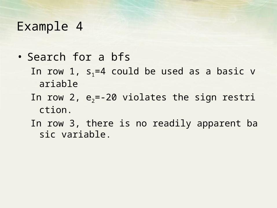
• Search for a bfsIn row 1, s1=4 could be used as a basic variable

In row 2, e2=-20 violates the sign restriction.

In row 3, there is no readily apparent basic variable.

• Artificial variablesTo remedy this problem, we simply "invent" a basic feas

ible variable for each constraint that needs one. These variables are created by us and are not real variables, we call them artificial variables.

If an artificial variable is added to row i, we label it ai.

Example 4

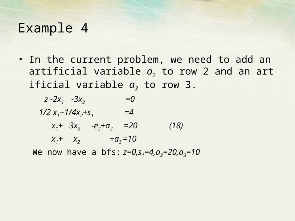
• In the current problem, we need to add an artificial variable a2 to row 2 and an artificial variable a3 to row 3.

z -2x1 -3x2 =0

1/2 x1+1/4x2+s1 =4

x1+ 3x2 -e2+a2 =20 (18)

x1+ x2 +a3 =10

We now have a bfs: z=0,s1=4,a2=20,a3=10

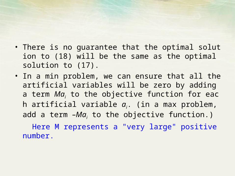
• There is no guarantee that the optimal solution to (18) will be the same as the optimal solution to (17).

• In a min problem, we can ensure that all the artificial variables will be zero by adding a term Mai to the objective function for each artificial variable ai. (in a max problem, add a term –Mai to the objective function.)

Here M represents a "very large" positive number.

Example 4

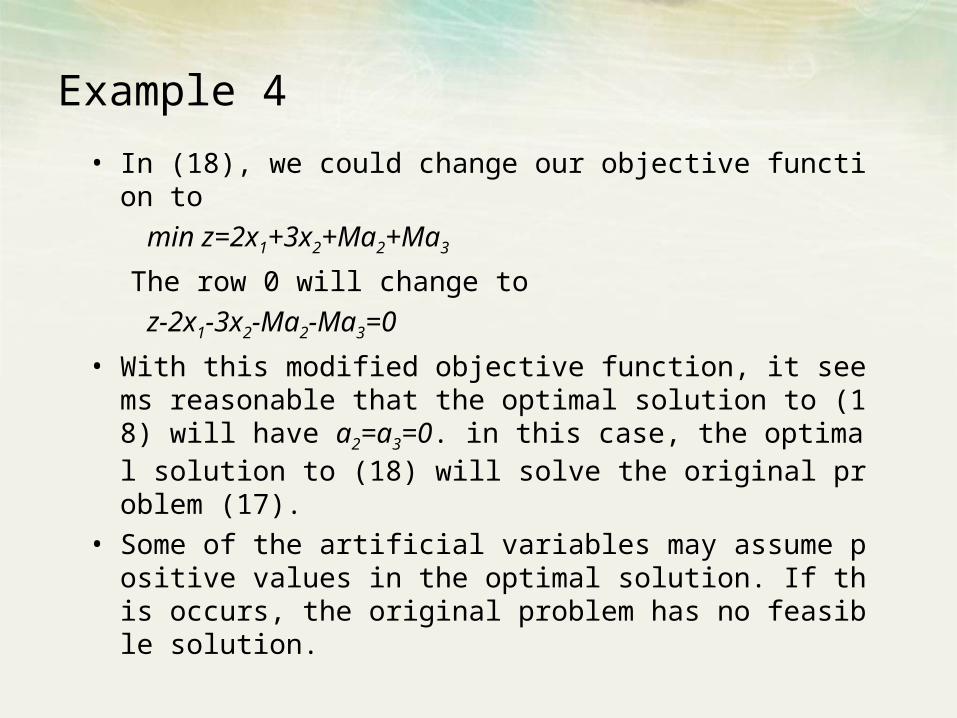
• In (18), we could change our objective function to

min z=2x1+3x2+Ma2+Ma3

The row 0 will change to

z-2x1-3x2-Ma2-Ma3=0

• With this modified objective function, it seems reasonable that the optimal solution to (18) will have a2=a3=0. in this case, the optimal solution to (18) will solve the original problem (17).

• Some of the artificial variables may assume positive values in the optimal solution. If this occurs, the original problem has no feasible solution.

Description of big M method

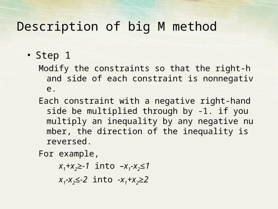
• Step 1Modify the constraints so that the right-hand side of

each constraint is nonnegative.

Each constraint with a negative right-hand side be multiplied through by -1. if you multiply an inequality by any negative number, the direction of the inequality is reversed.

For example,

x1+x2≥-1 into –x1-x2≤1

x1-x2≤-2 into -x1+x2≥2

Description of big M method

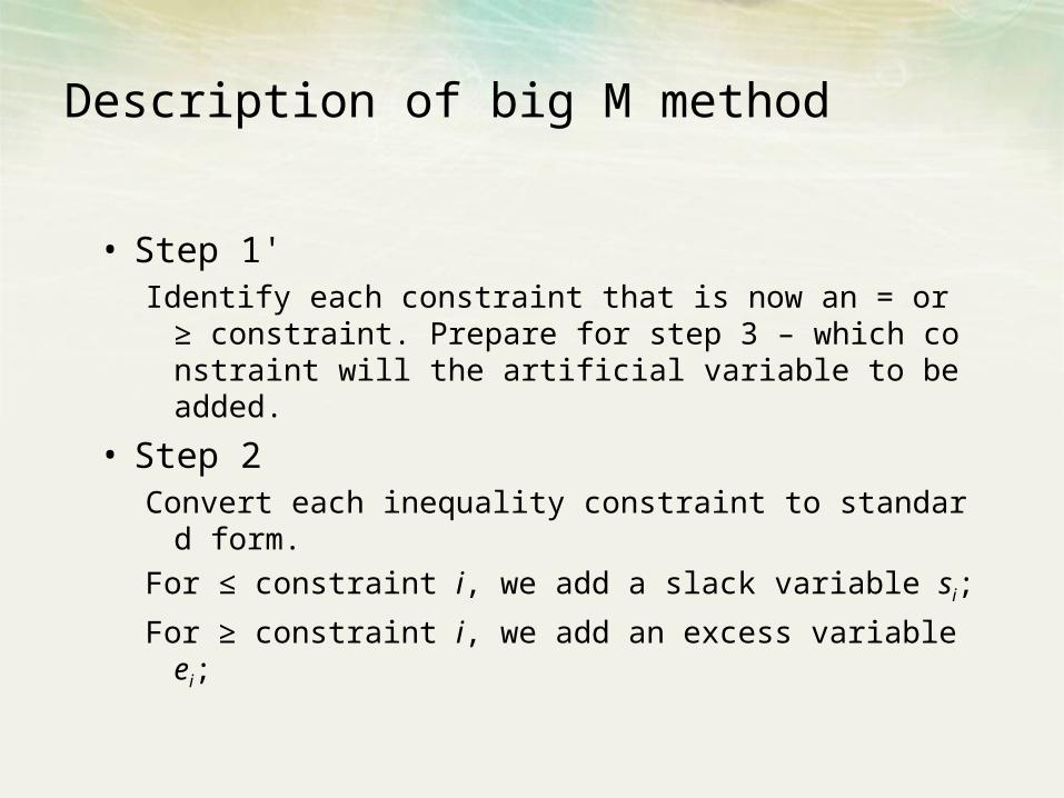
• Step 1'Identify each constraint that is now an = or ≥ constr

aint. Prepare for step 3 – which constraint will the artificial variable to be added.

• Step 2Convert each inequality constraint to standard form.

For ≤ constraint i, we add a slack variable si;

For ≥ constraint i, we add an excess variable ei;

Description of big M method

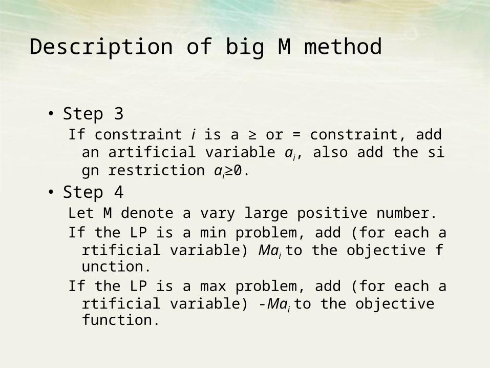
• Step 3If constraint i is a ≥ or = constraint, add an artificial v

ariable ai, also add the sign restriction ai≥0.

• Step 4Let M denote a vary large positive number.If the LP is a min problem, add (for each artificial var

iable) Mai to the objective function.If the LP is a max problem, add (for each artificial va

riable) -Mai to the objective function.

Description of big M method

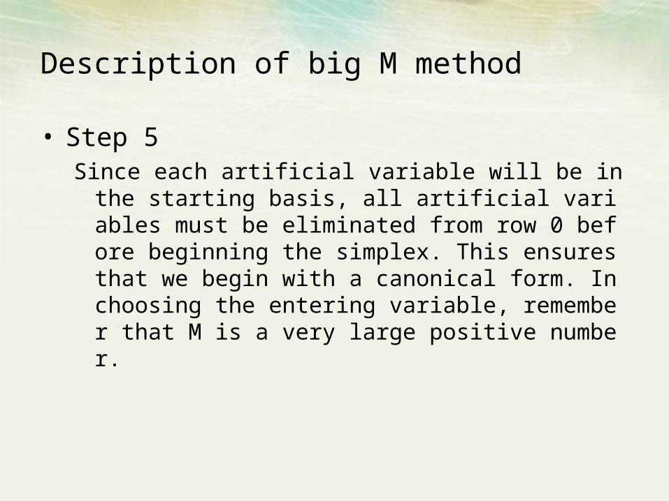
• Step 5Since each artificial variable will be in the starting basis,

all artificial variables must be eliminated from row 0 before beginning the simplex. This ensures that we begin with a canonical form. In choosing the entering variable, remember that M is a very large positive number.

Description of big M method

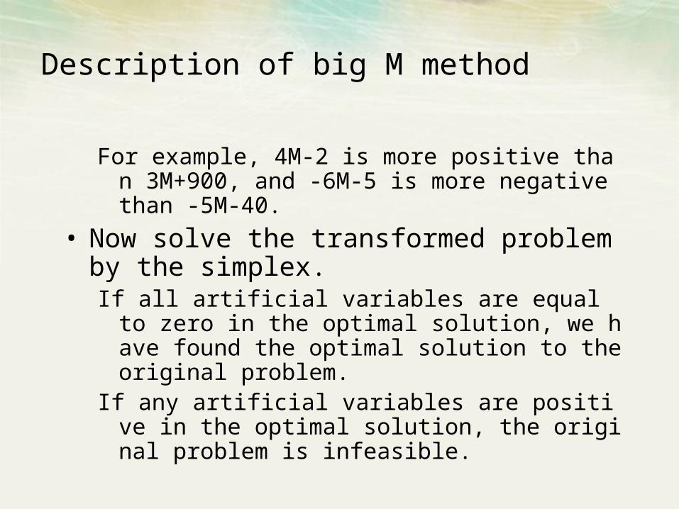
For example, 4M-2 is more positive than 3M+900, and -6M-5 is more negative than -5M-40.

• Now solve the transformed problem by the simplex. If all artificial variables are equal to zero in the optim

al solution, we have found the optimal solution to the original problem.

If any artificial variables are positive in the optimal solution, the original problem is infeasible.

Example 4 (continued)

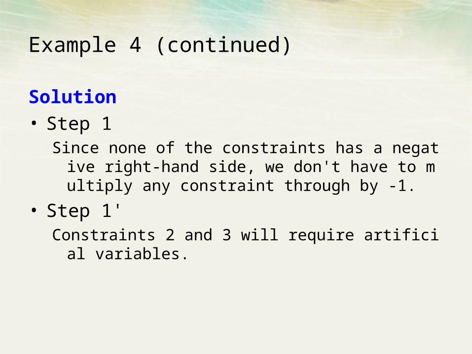
Solution• Step 1

Since none of the constraints has a negative right-hand side, we don't have to multiply any constraint through by -1.

• Step 1'Constraints 2 and 3 will require artificial variables.

Example 4 (continued)

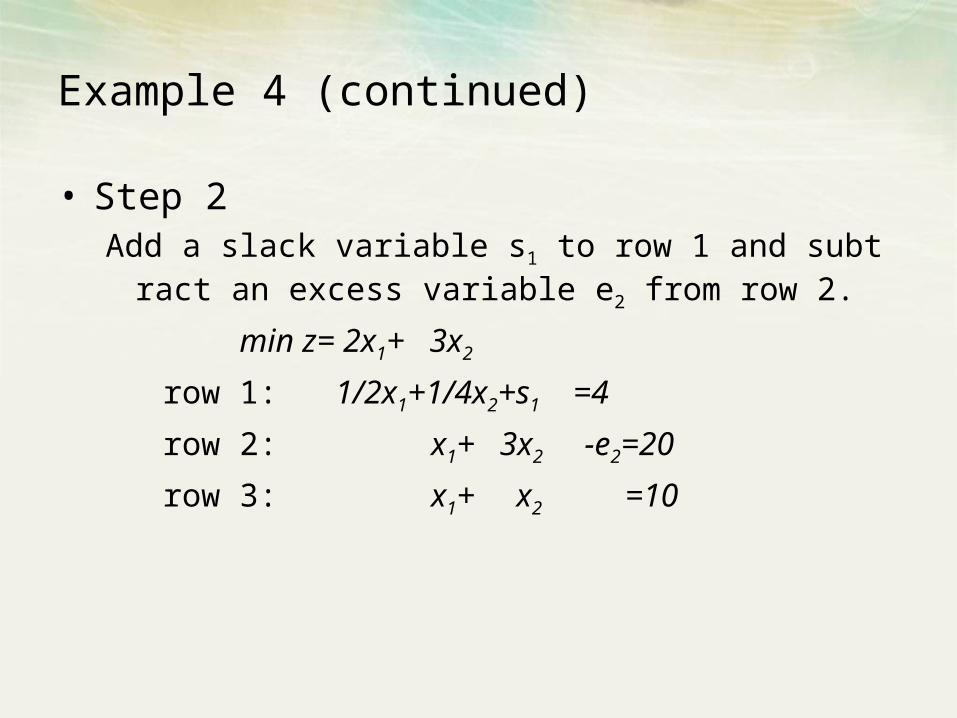
• Step 2Add a slack variable s1 to row 1 and subtract an excess

variable e2 from row 2.

min z= 2x1+ 3x2

row 1: 1/2x1+1/4x2+s1 =4

row 2: x1+ 3x2 -e2=20

row 3: x1+ x2 =10

Example 4 (continued)

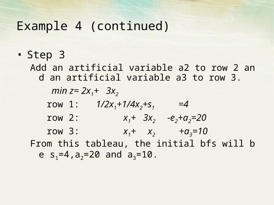
• Step 3Add an artificial variable a2 to row 2 and an artificial vari

able a3 to row 3.

min z= 2x1+ 3x2

row 1: 1/2x1+1/4x2+s1 =4

row 2: x1+ 3x2 -e2+a2=20

row 3: x1+ x2 +a3=10

From this tableau, the initial bfs will be s1=4,a2=20 and a

3=10.

Example 4 (continued)

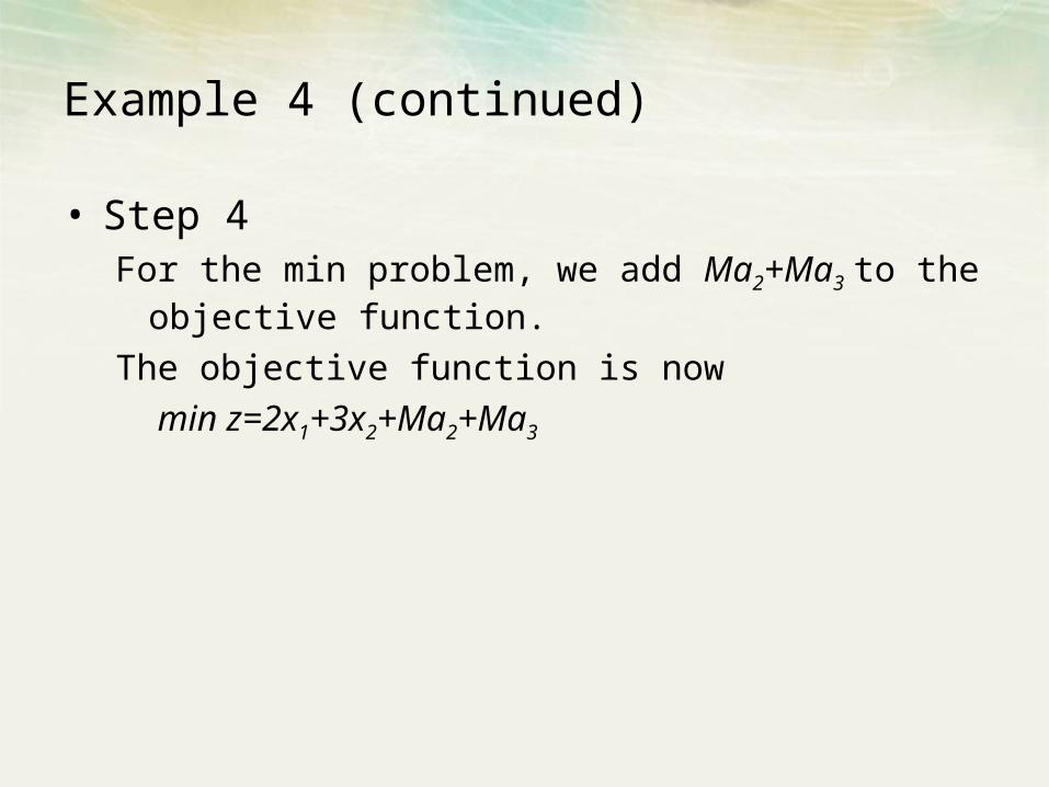
• Step 4For the min problem, we add Ma2+Ma3 to the objective f

unction.

The objective function is now

min z=2x1+3x2+Ma2+Ma3

Example 4 (continued)

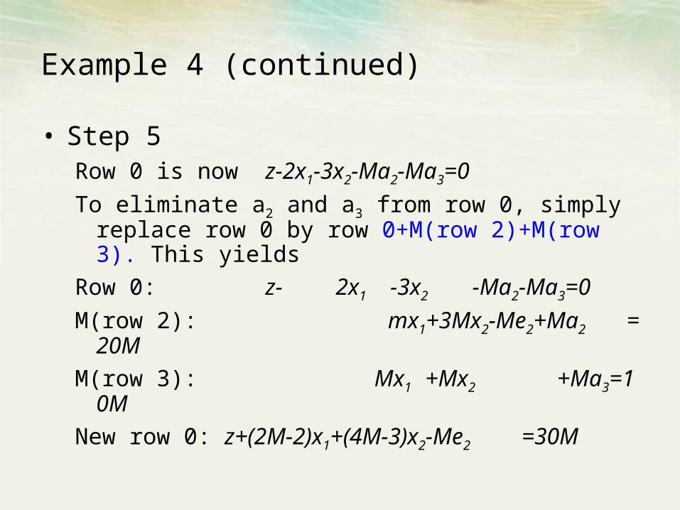
• Step 5Row 0 is now z-2x1-3x2-Ma2-Ma3=0

To eliminate a2 and a3 from row 0, simply replace row 0 by row 0+M(row 2)+M(row 3). This yields

Row 0: z- 2x1 -3x2 -Ma2-Ma3=0

M(row 2): mx1+3Mx2-Me2+Ma2 =20M

M(row 3): Mx1 +Mx2 +Ma3=10M

New row 0: z+(2M-2)x1+(4M-3)x2-Me2 =30M

Example 4 (continued)

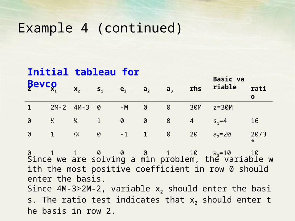
z x1 x2 s1 e2 a2 a3 rhs

Basic variable ratio

1 2M-2 4M-3 0 -M 0 0 30M z=30M

0 ½ ¼ 1 0 0 0 4 s1=4 16

0 1 ③ 0 -1 1 0 20 a2=20 20/3*

0 1 1 0 0 0 1 10 a3=10 10

Initial tableau for Bevco

Since we are solving a min problem, the variable with the most positive coefficient in row 0 should enter the basis.Since 4M-3>2M-2, variable x2 should enter the basis. The ratio test indicates that x2 should enter the basis in row 2.

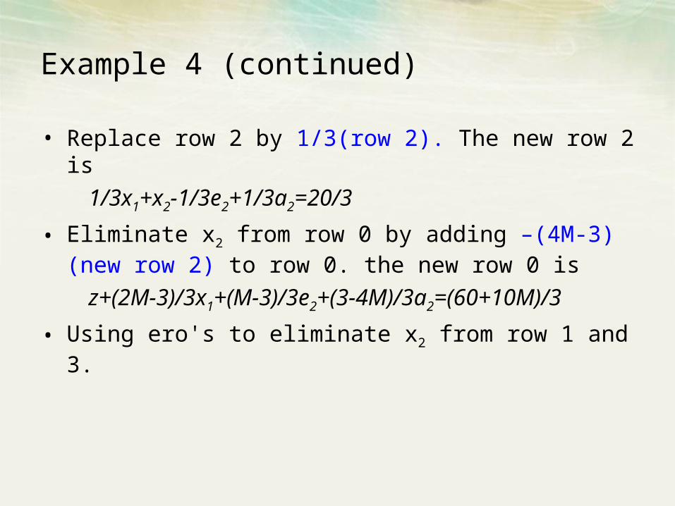
Example 4 (continued)

• Replace row 2 by 1/3(row 2). The new row 2 is

1/3x1+x2-1/3e2+1/3a2=20/3

• Eliminate x2 from row 0 by adding –(4M-3)(new row 2) to row 0. the new row 0 is

z+(2M-3)/3x1+(M-3)/3e2+(3-4M)/3a2=(60+10M)/3

• Using ero's to eliminate x2 from row 1 and 3.

Example 4 (continued)

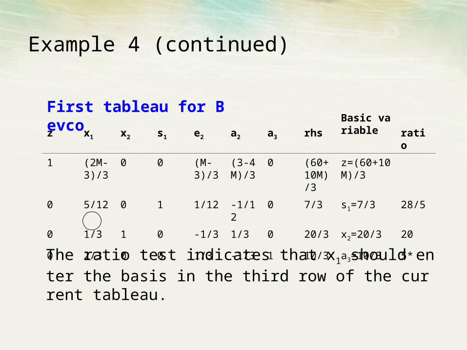
z x1 x2 s1 e2 a2 a3 rhs

Basic variable ratio

1 (2M-3)/3

0 0 (M-3)/3

(3-4M)/3

0 (60+10M)/3

z=(60+10M)/3

0 5/12 0 1 1/12 -1/12 0 7/3 s1=7/3 28/5

0 1/3 1 0 -1/3 1/3 0 20/3 x2=20/3 20

0 2/3 0 0 1/3 -1/3 1 10/3 a3=10/3 5*

First tableau for Bevco

The ratio test indicates that x1 should enter the basis in the third row of the current tableau.

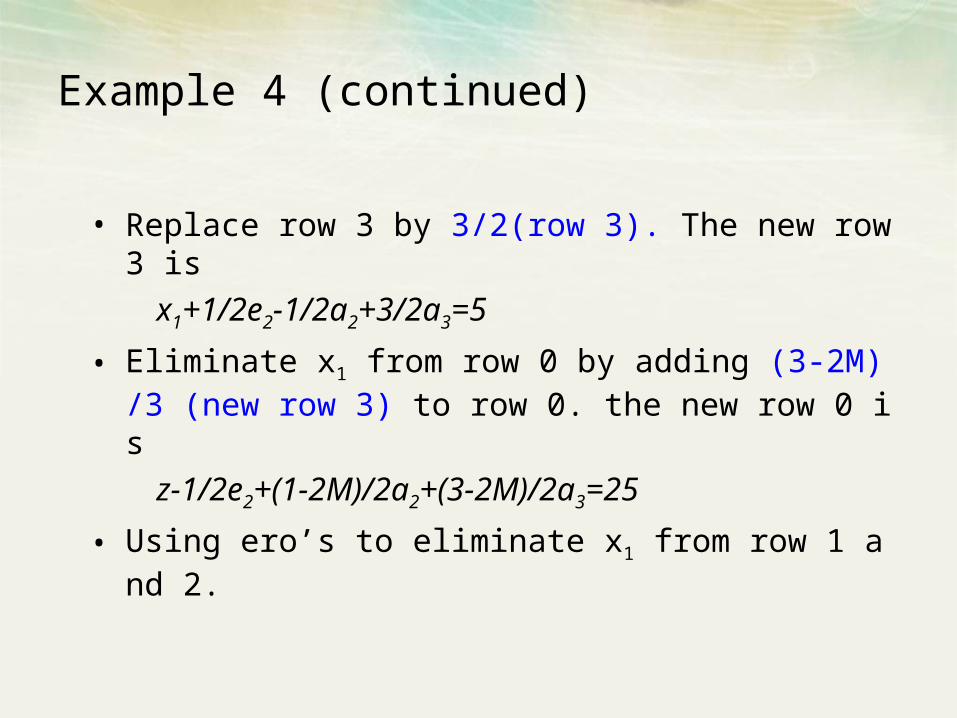
Example 4 (continued)

• Replace row 3 by 3/2(row 3). The new row 3 is

x1+1/2e2-1/2a2+3/2a3=5

• Eliminate x1 from row 0 by adding (3-2M)/3 (new row 3) to row 0. the new row 0 is

z-1/2e2+(1-2M)/2a2+(3-2M)/2a3=25

• Using ero’s to eliminate x1 from row 1 and 2.

Example 4 (continued)

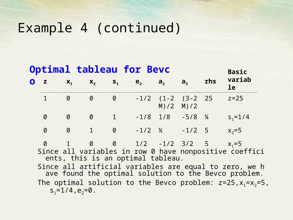
Since all variables in row 0 have nonpositive coefficients, this is an optimal tableau.

Since all artificial variables are equal to zero, we have found the optimal solution to the Bevco problem.

The optimal solution to the Bevco problem: z=25,x1=x2=5, s1=1/4,e2=0.

z x1 x2 s1 e2 a2 a3 rhs

Basic variable

1 0 0 0 -1/2 (1-2M)/2

(3-2M)/2

25 z=25

0 0 0 1 -1/8 1/8 -5/8 ¼ s1=1/4

0 0 1 0 -1/2 ½ -1/2 5 x2=5

0 1 0 0 1/2 -1/2 3/2 5 x1=5

Optimal tableau for Bevco

Example 4 (continued)

Note

• The a2 column could have been dropped after a2 left the basis (at the conclusion of the first pivot), and the a3 column could have been dropped after a3 left the basis( at the conclusion of the second pivot).

Summary

• If any artificial variable is positive in the optimal Big M tableau, the original LP has no feasible solution.

• When the Big M method is used, it is difficult to determine how large M should be. Generally, M is chosen to be at least 100 times larger than the largest coefficient in the original objective function.