The benefits of allowing heteroscedastic stochastic distributions in multiple discrete-continuous choice models

Contents lists available at ScienceDirect

The Journal of Choice Modelling

The Journal of Choice Modelling 9 (2013) 39–56

1755-53http://d

n CorrE-m1 Te

journal homepage: www.elsevier.com/locate/jocm

The benefits of allowing heteroscedastic stochastic distributionsin multiple discrete-continuous choice models

Sujan Sikder a,1, Abdul Rawoof Pinjari b,n

a Transportation Systems Modeler, Parsons Brinckerhoff, 400 SW Sixth Avenue, Suite 802, Portland, OR 97204, USAbDepartment of Civil & Environmental Engineering, University of South Florida, 4202 E. Fowler Ave., ENB 118, Tampa, FL 33620, USA

a r t i c l e i n f o

Available online 22 January 2014

Keywords:Discrete-continuous choice modelsMultiple discretenessHeteroscedasticityDistributional assumptionsTime use behaviorSpatial transferability

45/$ - see front matter & 2013 Elsevier Ltd.x.doi.org/10.1016/j.jocm.2013.12.003

esponding author. Tel.: þ1 813 974 9671; faail addresses: [email protected] (S. Sikdel.: þ1 813 507 3953; fax: þ1 813 974 2957.

a b s t r a c t

This paper investigates the benefits of incorporating heteroscedastic stochastic distribu-tions in random utility maximization-based multiple discrete-continuous (MDC) choicemodels. To this end, first, a Multiple Discrete-Continuous Heteroscedastic Extreme Value(MDCHEV) model is formulated to allow heteroscedastic extreme value stochasticdistributions in MDC models. Next, an empirical analysis of individuals0 daily time usechoices is carried out using data from the National Household Travel Survey (NHTS) forthree geographical regions in Florida. A variety of different MDC model structures areestimated: (a) the Multiple Discrete-Continuous Extreme Value (MDCEV) model withindependent and identically distributed (IID) extreme value error structure, (b) theMDCHEV model, (c) the mixed-MDCEV model that allows heteroscedasticity by mixinga heteroscedastic distribution over an IID extreme value kernel, (d) the MDC generalizedextreme value (MDCGEV) model that allows inter-alternative correlations using themultivariate extreme value error structure, (e) the mixed-MDCEV model that allowsinter-alternative correlations using common mixing distributions across choice alterna-tives, and (f) the mixed-MDCEV model that allows both heteroscedasticity and inter-alternative correlations. Among all these model structures, the MDCHEV model providedthe best fit to the current empirical data. Further, heteroscedasticity was prominent whileno significant inter-alternative correlations were found. Specifically, the MDCHEV para-meter estimates revealed the significant presence of heteroscedasticity in the randomutility components of different activity type choice alternatives. On the other hand, theMDCEV model resulted in inferior model fit and systematic discrepancies between theobserved and predicted distributions of time allocations, which can be traced to the thickright tail of the type-1 extreme value distribution. The MDCHEV model addressed theseissues to a considerable extent by allowing tighter stochastic distributions for certainchoice alternatives, thanks to its accommodation of heteroscedasticity among randomutility components. Furthermore, spatial transferability assessments using differenttransferability metrics also suggest that the MDCHEV model clearly outperformed theMDCEV model.

& 2013 Elsevier Ltd. All rights reserved.

All rights reserved.

x: þ1 813 974 2957.r), [email protected] (A.R. Pinjari).

www.sciencedirect.com/science/journal/17555345

www.elsevier.com/locate/jocm

http://dx.doi.org/10.1016/j.jocm.2013.12.003



mailto:[email protected]

mailto:[email protected]


S. Sikder, A.R. Pinjari / Journal of Choice Modelling 9 (2013) 39–5640

1. Introduction

1.1. Background

Numerous consumer choices are characterized by “multiple discreteness” where consumers can potentially choosemultiple alternatives from a set of discrete alternatives available to them. Along with such discrete-choice decisions ofwhich alternative(s) to choose, consumers typically make continuous-quantity decisions on how much of each chosenalternative to consume. Such multiple discrete-continuous (MDC) choices are being increasingly recognized and analyzed ina variety of scientific fields, including transportation, environmental economics, and marketing. Examples include(1) individuals0 daily time-use choices, which involve decisions to engage in different types of activities in a day alongwith the allocation of available time to each activity, (2) households0 recreational destination choices and time allocation tothe chosen destinations over a season, and (3) grocery shoppers0 brand choice and purchase quantity decisions.

A variety of approaches have been used in the literature to model MDC choices. Among these, a particularly attractiveapproach is based on the classical microeconomic consumer theory of constrained utility maximization. Specifically,consumers are assumed to optimize a direct utility function UðxÞ over a set of non-negative consumption quantitiesx¼ ðx1; :::; xk; :::; xK Þ subject to a linear budget constraint, as

Max UðxÞ such that x � p ¼ y and xkZ08k¼ 1;2; :::;K ð1Þ

In the above equation, UðxÞ is a quasi-concave, increasing and continuously differentiable utility function with respect to theconsumption quantity vector x, p is a vector of unit prices for all goods, and y is a budget for total expenditure. Anincreasingly popular approach for deriving the demand functions from the utility maximization problem in Eq. (1), due toHanemann (1978) and Wales and Woodland (1983), is based on the application of Karush–Kuhn–Tucker (KKT) conditions ofoptimality with respect to the consumption quantities. Since the utility function is assumed to be randomly distributed overthe population, the KKT conditions are also randomly distributed and form the basis for deriving the probability expressionsfor consumption patterns.

Over the past decade, the above-discussed KKT approach has received significant attention for the analysis of MDCchoices. A stream of research in environmental economics (Phaneuf et al., 2000; von Haefen et al., 2004; von Haefen andPhaneuf, 2005; Phaneuf and Smith, 2005; Vasquez-Lavin and Hanemann, 2009) advanced the approach to modelindividuals0 recreational demand choices for non-market valuation of environmental goods. Several studies in marketingresearch (Kim et al., 2002; Satomura et al., 2011) employed the approach to model situations when consumers purchase avariety of brands of a product (e.g., yogurt). In the transportation field, the multiple discrete-continuous extreme value(MDCEV) model formulated by Bhat (2005) and enlightened further by Bhat (2008) lead to an increased use of the KKTapproach for analyzing a variety of choices, including individuals0 activity participation and time-use (Bhat 2005; Habib andMiller, 2008; Pinjari et al., 2009; Chikaraishi et al., 2010; You et al., 2013), household vehicle ownership and usage (Ahnet al., 2008; Bhat et al., 2009; Jaggi et al., 2013), long-distance leisure destination choices (Van Nostrand et al., 2013), energyconsumption choices (Pinjari and Bhat, 2011; Frontuto, 2011; Yu et al., 2012) and builders0 land-development choices (Kazaet al., 2012; Farooq et al., 2013). Clever use of stochastic specifications has led to model formulations with closed-formlikelihood expressions. Specifically, consider an additive utility form, as follows:

Uðx1; :::; xK Þ ¼ ∑K

k ¼ 1UðxkÞ ¼ ∑

K

k ¼ 1f ðuðxkÞ; εkÞ ð2Þ

In the above equation, UðxkÞ is a random sub-utility function for good k, representing the utility derived from consuming xkamount of good k, and expressed as a combination of a deterministic component uðxkÞ and a random component εk asUðxkÞ ¼ f ðuðxkÞ; εkÞ. Assuming that the random components (εk) enter the sub-utility functions UðxkÞ in a multiplicativefashion, as UðxkÞ ¼ uðxkÞ � eεk , and are type-1 extreme value and independent and identically distributed (IID) across thechoice alternatives leads to a very simple and elegant consumption probability expression (Bhat, 2005), making it easy forparameter estimation. In addition, computationally efficient procedures are now available for using these model systems forforecasting and policy evaluation (see von Haefen et al. (2004) and Pinjari and Bhat (2011)). Thanks to these advances, KKT-based MDC models are being increasingly used in empirical research and have begun to be used in operational travelforecasting models.

1.2. Gaps in literature relevant to this paper

Recent research in this area has started to enhance the basic formulation in Eq. (1) along three specific directions:(a) toward more flexible, non-additively separable functional forms for the utility specification so as to accommodate richcomplementarity and substitution patterns in consumption (Vasquez-Lavin and Hanemann, 2009; Bhat et al., 2013a),(b) toward greater flexibility in the specification of the constraints faced by the consumer, such as multiple linear budgetconstraints as opposed to a single constraint (Satomura et al., 2011; Castro et al., 2012; Pinjari and Sivaraman, 2013), and(c) toward more flexible stochastic specifications for the random utility functions. The reader is referred to Pinjari et al.(2013) for a more detailed discussion of recent advances along the first two directions.

S. Sikder, A.R. Pinjari / Journal of Choice Modelling 9 (2013) 39–56 41

Within the context of stochastic specifications in KKT models, recent work has been geared toward relaxing the IIDassumption of random utility components, in the following ways: (1) the specification of multivariate extreme value (MEV)distributions as opposed to IID extreme value distributions, which leads to the multiple discrete-continuous generalizedextreme value (MDCGEV) structure (Pinjari and Bhat, 2010; Pinjari, 2011); (2) the specification of multivariate normal(MVN) distribution, which leads to the multiple discrete-continuous probit (MDCP) structure (Kim et al., 2002; Bhat et al.,2013b), and (3) the specification of additional error components mixed over an IID extreme value distributed kernel, whichleads to the mixed-MDCEV structure (Bhat, 2005; Bhat and Sen, 2006; Spissu et al., 2009; Chikaraishi et al., 2010).

A number of efforts to relax the IID assumption have been made in the context of relaxing the independently distributedassumption, by allowing correlations between the random utility components of different choice alternatives (either byemploying the MEV or MVN distributions or by employing the mixed-MDCEV structure). Such correlations help inaccommodating flexible substitution patterns between the consumptions of different choice alternatives (Pinjari and Bhat,2010). In addition, positive correlations between alternatives can capture the possibility that the consumptions of groups ofalternatives can be complementary to each other in that an increase in the consumption of one alternative increases theconsumption of other alternatives.

A handful of studies relax the identically distributed assumption by allowing for inter-alternative variations in thestochastic distributions (i.e., heteroscedastic distributions). Specifically, Bhat and Sen (2006) use the mixed-MDCEVstructure to accommodate heteroscedasticity across choice alternatives. Spissu et al. (2009) also used the mixed-MDCEVstructure, albeit with panel data, to accommodate variations in the influence of unobserved factors within and acrossindividuals (i.e., inter-individual and intra-individual variations). In another notable study, Chikaraishi et al. (2010) use themixed-MDCEV structure to accommodate variations in unobserved influences at multiple levels, including intra-individualvariation, inter-individual variation, inter-household variation, and temporal and spatial variation. Both Spissu et al. (2009)and Chikaraishi et al. (2010) allow for the unobserved variations to be different across the different choice alternatives,thereby allowing for heteroscedasticity across choice alternatives. In all these studies, the primary reason for accommodat-ing heteroscedasticity across choice alternatives is to recognize the differences in the variation of unobserved influences onthe preferences for different choice alternatives. As often cited in the literature, doing so helps in improving the model fit tothe data as well as accommodates the influence of heteroscedastic random variance on the elasticity effects of alternativeattributes. For instance, the self-price elasticity estimate of a choice alternative is dampened by the variance in its randomutility component (Bhat and Sen, 2006). However, what has been unknown (and unexplored) so far is the potentialinfluence of heteroscedasticity across choice alternatives on the distributions of the consumptions implied by a KKT demandsystem such as the MDCEV model. It is this specific aspect that the current paper contributes to.

Another line of recent research has been on evaluating the predictions obtained from KKT-based MDC models. A firststep in this direction is the study by Jaggi et al. (2013), who analyzed the residuals between observed consumptions in theestimation data and predicted consumptions (on the same data) using the MDCEV model. In a recent study, Sikder andPinjari (2013) compared the predictions from the MDCEV model with those observed in the estimation data. Their empiricalanalysis reveals both strengths and weaknesses of the MDCEV formulation in predicting the aggregate-level discrete choicesand continuous consumption quantities in the context of individuals0 daily time-use decisions. Specifically, they reportedthat the MDCEV model performs very well in predicting the aggregate-level discrete choices observed in the estimation data(i.e., the market shares for each choice alternative). However, the continuous consumption quantities (i.e., daily timeallocations) were reported to have been overestimated for certain alternatives and underestimated for other alternatives,when compared to the average consumptions in the estimation data. Alluding to the possibility that this problem could beattributed to the fat right tail of the extreme value distributions assumed in the MDCEV model, Sikder and Pinjari (2013)identify a research need to explore alternative distributional assumptions to overcome the issue. In the current paper, weexplore the benefits of incorporating heteroscedasticity in the stochastic distributions across different choice alternatives inaddressing the afore-mentioned prediction related issues of the MDCEV model.

Both the mixed-MDCEV and MDCP approaches can be used to relax the assumption of identically distributed errors.The advantage of both these approaches is that they are very general; the analyst can allow for correlated and non-identically (or heteroscedastically) distributed random utility terms simultaneously, while also allowing random coefficientson explanatory variables and recognizing correlations across observations. However, both the approaches have their owndrawbacks. The likelihood function of the mixed-MDCEV formulation for allowing heteroscedasticity is a multidimensionalintegral of as many dimensions as the number of heteroscedastic choice alternatives. The dimensionality of the integralincreases further when other features such as inter-alternative correlations and random coefficients are incorporated (alongwith heteroscedasticity) using the mixed-MDCEV approach. This integral cannot be evaluated analytically and necessitatesthe use of computationally intensive simulation techniques as the dimensionality of integration increases beyond a modestnumber. The typically used approach to estimating the mixed-MDCEV models is the maximum simulated likelihood (MSL)method, where the likelihood is simulated using pseudo-Monte Carlo or quasi-Monte Carlo simulation. The desirableasymptotic properties of the MSL estimator come with a computational cost, because the number of simulation draws oughtto increase faster than the square root of the number of observations in the estimation sample. As is widely noted in theliterature (Train, 2009), the accuracy of such simulation techniques degrades quickly at high dimensions of integrationunless a large number of simulation draws is used. Even if using a large number of draws is not impossible, it certainlyincreases the model estimation time, thereby discouraging the analyst from exploring a variety of alternative empiricalspecifications. Another important issue that has not received due attention in the literature (but see Bhat (2011)) is the


accuracy of the covariance matrix of the MSL estimator (not just the accuracy of the simulator itself), which is important forgood statistical inference. As stated in Bhat (2011), simulating the log-likelihood function with even three to four decimalplaces of accuracy in the probabilities might not be sufficient for an accurate estimation of the covariance matrix of the MSLsimulator. The implication is that the likelihood function needs to be simulated with a very high level of accuracy andprecision (Bhat, 2011), which further increases the computational intensity. Finally, another drawback with the simulationmethods is that parameter (un)identification issues arise quickly when the number of random coefficients to be estimatedincreases beyond a modest number. Suffice it to say that while the mixed-MDCEV approach is valuable for simultaneouslyallowing a variety of features such as inter-alternative correlations and heteroscedasticity, it is worth incorporating thesefeatures using techniques that help reduce the dimensionality of integration in the likelihood function. For example, theMDCGEV structure (Pinjari, 2011) can be used to allow inter-alternative correlations while retaining the closed-form of thelikelihood expressions. Along similar lines, it would be useful to explore a simpler approach to incorporating hetero-scedasticity in MDC models. One possibility of doing so, as discussed in the next section, is to use heteroscedastic extremevalue (HEV) distributions in lieu of the homoscedastic extreme value distributions used in the MDCEV model.

As mentioned earlier, the MDCP approach can also be used to allow heteroscedasticity. The MDCP approach, similar tothe mixed-MDCEV approach, leads to multi-dimensional integrals (in the likelihood function) that are not analyticallytractable. An advantage of this approach is that the dimensionality of integration is always equal to one less than thenumber of choice alternatives, regardless of the number of random parameters and the presence of heteroscedasticity andinter-alternative correlations. This property is advantageous for situations with small to medium number of choicealternatives. The MDCP models are typically estimated using the GHK simulator to evaluate the integral appearing in thelikelihood function (see Kim et al., 2002). However, in addition to being computationally intensive, the GHK simulator is noteasy to implement, a reason why most analysts resort to the mixed-MDCEV approach. More recently, Bhat et al. (2013b)demonstrated the benefits of an analytic approximation method to evaluate the integrals in the MDCP structure. Thisdevelopment might make it simpler to use MDCP models in empirical research.

1.3. Current research

In view of the above discussed gaps in the literature, the primary objective of this paper is to investigate the benefits ofincorporating heteroscedastic stochastic distributions in KKT-based MDC choice models. To this end, we first formulate aMultiple Discrete-Continuous Heteroscedastic Extreme Value (MDCHEV) model that employs heteroscedastic extreme value(HEV) distributed random utility components in KKT-based MDC models. The HEV distribution was originally used by Bhat(1995) for modeling single discrete choice situations. One advantage of the proposed MDCHEV approach over the other twoapproaches (i.e., mixed-MDCEV and MDCP) is that the resulting likelihood function is a uni-dimensional integral that can beeasily and accurately evaluated using quadrature methods; a reason why Bhat (1995) used it. Note, however, that theMDCHEV structure does not accommodate either inter-alternative correlations or random coefficients on explanatoryvariables. As discussed earlier, the mixed-MDCEV and the MDCP approaches are more general than the MDCHEV as they cansimultaneously accommodate heteroscedasticity, inter-alternative correlations, and random coefficients. In practice,however, it can be very difficult to empirically identify a large number of random parameters needed to accommodateall these different features in the mixed-MDCEV model, especially with cross-sectional datasets. To overcome this issue, onecan potentially formulate a mixed-MDCHEV model that superimposes a mixing distribution over a HEV kernel toaccommodate inter-alternative correlations and random coefficients along with heteroscedasticity. Alternatively, one canconceive of a mixed-MDCHGEV model that is based on a heteroscedastic generalized extreme value (HGEV) kernel to allowboth heteroscedasticity and inter-alternative correlations, and superimposes a mixing distribution over the HGEV kernel toallow random coefficients. However, these extensions as well as the MDCP approach are beyond the scope of this paper.2

In addition to the formulation of the MDCHEV model, an empirical analysis is presented in the context of modelingindividuals0 daily time-use choices using data from the 2009 National Household Travel Survey (NHTS) from Florida. Theempirical analysis proceeds in two stages. In the first stage, a series of model estimations is carried out to select the bestfitting MDC model structure for the current empirical data. Specifically, the following six different model structures areestimated: (1) The MDCEV model with IID extreme value stochastic distributions; (2) the mixed-MDCEV model toaccommodate heteroscedasticity across choice alternatives; (3) the MDCHEV model; (4) the mixed MDCEV model toaccommodate inter-alternative correlations; (5) the MDCGEV model to incorporate inter-alternative correlations usingclosed-form probability expressions; and (6) the mixed-MDCEV model to accommodate both inter-alternative correlationsand heteroscedasticity. As will be revealed in the empirical results section, in the current empirical context, inter-alternativecorrelations were not significant but heteroscedasticity was prominent. Further, among all the above six model structures,the MDCHEV structure provided the best fit to the data, with goodness-of-fit measures far better than the mixed-MDCEVstructure. In the second stage, we focus on assessing the benefits of incorporating heteroscedastic stochastic distributions inthe context of modeling individuals0 daily time-use choices. Considering the findings in the first stage of the empirical

2 In this context, we identify the following potentially fruitful avenues for future research: (1) exploration of the pros and cons of alternativeapproaches (e.g., mixed-MDCEV, MDCP, and mixed-MDCHGEV) to simultaneously accommodate inter-alternative correlations, heteroscedasticity, randomcoefficients, and (2) assessment of the relative importance of each of these unobserved effects in different empirical contexts.


analysis, we compare the prediction performance of the MDCEV and MDCHEV model structures. In these comparisons, wefirst demonstrate that the distributions of the MDCEV-predicted continuous quantity decisions for certain choicealternatives can potentially have longer right tails than the observed distributions, thereby implying overestimation ofthe continuous quantity predictions for those choice alternatives. We discuss how this problem is related to the fat right tailof the IID extreme value distributions assumed in the MDCEV model. We also demonstrate empirically that allowing forheteroscedasticity through the MDCHEV model helps in addressing this problem to a considerable extent. This is becausethe heteroscedastic model results in smaller variances (hence tighter distributions) for the random utility components of thechoice alternatives for which the MDCEV model over-predicts the continuous quantity choices. Such tightly distributedrandom utility components, as will be demonstrated later in the paper, reduce the probability of unreasonably largecontinuous quantity predictions. In addition to comparing the in-sample prediction performance of the MDCEV andMDCHEV models, we also compare the out-of-sample prediction performance by assessing the spatial transferability of themodels among different geographical regions in Florida.

The remainder of the paper is organized as follows. The next section presents the structure of the MDCHEV model andoutlines the estimation procedure. Section 3 overviews the empirical data and geographical contexts considered for theempirical analysis. Section 4 presents the empirical results. Section 5 summarizes and draws conclusions from the paper.

2. The MDCHEV model

2.1. Model formulation

Consider the following random utility function proposed by Bhat (2008) for modeling multiple discrete-continuouschoice situations:

UðtÞ ¼ ψ1 ln t1þ ∑K

k ¼ 2fψkγk lnððtk=γkÞþ1Þg ð3Þ

In the above function, UðtÞ is the total utility derived by an individual from his/her daily time-use. It is the sum of sub-utilities derived from allocating time (tk) to each of the activity types k (k¼1, 2, …, K). Individuals are assumed to make theiractivity participation and time-use decisions such that they maximize UðtÞ subject to a linear budget constraint∑ktk ¼ T ,where T is the total available time budget. Note that the subscript for the individual is suppressed for simplicity in notation.

Within the utility function in Eq. (3), ψk, called the baseline marginal utility for alternative k, is the marginal utility oftime allocation to activity k at the point of zero time allocation. ψk governs the discrete choice decisions in that an activitytype with greater baseline marginal utility is more likely to be chosen than the other activities. γk accommodates cornersolutions (i.e., the possibility of not choosing an alternative). Both ψk and γk accommodate differential satiation effects(diminishing marginal utility with increasing consumption) for different activity types. Thus, both these parametersinfluence the time allocation decisions. Specifically, a greater value of either ψk or γk implies a larger allocation of time to thecorresponding activity. Note that the 1st alternative, designated as in-home activity, does not have a γk parameter since allindividuals in the data allocate some time to the in-home activity (i.e., there is no need of corner solutions for this activity).From now on, this alternative will be called the outside good, whereas all other activities (out-of-home activities) are calledinside goods.3

The influence of observed and unobserved individual characteristics and activity-travel environment (ATE) measures areaccommodated into the utility function as ψ1 ¼ expðε1Þ; ψk ¼ expðβ0zkþεkÞ; and γk ¼ expðθ0wkÞ;where zk and wk are observedsocio-demographic and ATE measures influencing the choice of and time allocation to activity k, β and θ are thecorresponding parameter vectors, and εk (k¼1, 2, …, K) is the random error term capturing unobserved and unmeasuredinfluences on the utility contribution of time allocation in activity type k. Note that ψ1 does not include any observedexplanatory variables as the coefficients of all explanatory variables for this alternative are normalized to zero foridentification purposes.

To obtain the optimal time allocations (tn1; tn

2; :::; tnK ), one can form the Lagrangian and derive the Karush–Kuhn–Tucker

(KKT) conditions of optimality (Bhat 2008). The Lagrangian function for the utility function and budget constraintconsidered in this study is

L¼ ψ1 ln t1þ ∑K

k ¼ 2fψkγk lnððtk=γkÞþ1Þg�λ ∑

K

k ¼ 1tk�T

" #ð4Þ

3 The outside good is a composite good that represents all goods other than the K-1 inside goods of interest to the analyst. The presence of the outsidegood helps ensure that the budget constraint is binding. Besides, the outside good helps in endogenously determining the total resource allocation for (ortotal consumption of) inside goods. It is not uncommon to treat the outside good as a numeraire with unit price, assuming that the prices andcharacteristics of the goods grouped into the outside category do not influence the choice and resource allocation among the inside goods (see Deaton andMuellbauer (1980)). Although the current empirical context is such that the outside good is an essential good (where all individuals consume some amountof it), it is not always necessary for the outside good to be specified as an essential good.


where λ is the Lagrangian multiplier associated with the budget constraint. The KKT conditions of optimality are

Vkþεk ¼ V1þε1 if tnk40; ðk¼ 2;3; ::::;KÞ

VkþεkoV1þε1 if tnk ¼ 0; ðk¼ 2;3; ::::;KÞ ð5Þwhere, V1 ¼ lnðtn1Þ; and Vk ¼ β0zkþ lnððtnk=γkÞþ1Þ; ðk¼ 2;3::::::;KÞ

The above stochastic KKT conditions form the basis for the derivation of likelihood expressions. In the general case, if thejoint probability density function of the εk terms is gðε1; ε2; :::; εkÞ, and if M alternatives are chosen out of the available Kalternatives, and if the consumptions of these M alternatives are ðtn1; tn2; tn3; :::; tnMÞ, as given in Bhat (2008), the jointprobability expression for this consumption pattern is as follows:

Pðtn1; tn2; tn3; :::; tnM ;0;0;0:::;0Þ ¼

J�� Z þ1

ε1 ¼ �1

Z V1 �VMþ 1 þ ε1

εMþ 1 ¼ �1::

Z V1 �Vk� 1 þ ε1

εk� 1 ¼ �1

Z V1 �Vk þ ε1

εk ¼ �1gðε1;V1�V2þε1;V1�V3þε1; :::;V1�VMþε1; εMþ1; εMþ2; :::; εK�1; εK Þ

dεk dεk�1:::dεMþ2 dεMþ1 dε1 ð6Þwhere J

�� is the determinant of a Jacobian whose elements are given by (see Bhat (2005))

Jih ¼∂ V1�Viþ1þε1� �

∂tnhþ1¼ ∂ V1�Viþ1

� �∂tnhþ1

; i;h¼ 1;2; :::;M�1 ð7Þ

For the MDCHEV model, we assume that the random components in the baseline marginal utilities of different choicealternatives are independent but heteroscedastically extreme value (HEV) distributed. Specifically, the random error term εkof each alternative k ðk¼ 1;2;3; ::::;KÞ is assumed to have a type-1 extreme value distribution with a location parameterequal to zero and a scale parameter equal to sk. With the HEV distribution, the probability expression in Eq. (6) becomes

Pðtn1; tn2; :::; tnM ;0; :::;0Þ ¼ J�� Z ε1 ¼ þ1

ε1 ¼ �1∏M

j ¼ 2

1sjg

V1�Vjþε1sj

� �( )� ∏

K

s ¼ Mþ1G

V1�Vsþε1ss

� �( )� g

ε1s1

� �d

ε1s1

� �ð8Þ

where g(.) and G(.) are the probability density function and cumulative distribution function, respectively, of the standardtype I extreme value distribution; Specifically, gðwÞ ¼ e�we�e�w

and GðwÞ ¼ e�e�w. If the scale parameters sk across all

alternatives are assumed to be equal, then the above expression simplifies to the closed-form MDCEV model derived by Bhat(2005).

2.2. Model estimation

The parameters of the MDCHEV model can be estimated using the familiar maximum likelihood procedure. However,there is no analytical form for the integral appearing in the probability expression of Eq. (8), which enters the likelihoodfunction. In this paper, we employ the Laguerre Gaussian Quadrature (Press et al., 1986) to compute the integral. To do so,define w¼ ε1

s1and u¼ e�w. These two equations can be combined to write ε1 ¼ �s1 ln u. Further, du

dw ¼ ddw ðe�wÞ ¼ �e�w or

dw¼ �ewdu. Now, the term g ε1s1

d ε1

s1

in Eq. (8) can be written as gðwÞ dw, which can further be expanded as

e�we�e�wdw. Substituting �ew du for dw and u for e�w, one can write g ε1

s1

d ε1

s1

¼ �e�u du. Finally, substituting

�s1 ln u for ε1 and �e�u du for g ε1s1

d ε1

s1

, the probability expression in Eq. (8) can be re-written as follows:

Pðtn1; tn2; tn3; :::; tnM ;0;0; :::;0Þ ¼ J�� Z 1

u ¼ 0f ðuÞe�u du ð9Þ

where f ðuÞ ¼ ∏Mj ¼ 2

1sjg V1 �Vj �s1 ln u

sj

h in o� ∏K

s ¼ Mþ1GV1 �Vs �s1 ln u

ss

h in oAccording to the Laguerre Gaussian Quadrature technique, the integral of the form in Eq. (9) can be approximated as a

summation of terms over a certain number (I) of support points as follows:Z 1

u ¼ 0f ðuÞe�u du� ∑

I

i ¼ 1wif ðuiÞ ð10Þ

where i is the support point at which the function f ðuiÞ is evaluated (support points are the roots of the Laguerre polynomialof order I) and wi is the weight or probability mass associated with support point i (see Press et al. (1986)). Since the integralbeing evaluated is uni-dimensional, the quadrature method is computationally efficient and accurate. In this paper,preliminary tests suggested that increasing the number of support points (I) beyond 15 did not increase the accuracy of theintegral or influence the final model results (log-likelihood function value and parameter estimates). Therefore, allestimations of MDCHEV models were performed using 15 support points to evaluate the integral in the likelihood function.The likelihood function was coded in the maximum likelihood estimation module of the GAUSS matrix programminglanguage.


Note that, since there is no variation in the prices of unit consumption of different activity alternatives in the currentempirical context, for identification purposes, at least one of the scale parameters need to be fixed to an arbitrary value(Bhat, 2008). It is convenient to fix the scale parameter of the essential outside good (in-home activity) to 1. Therefore, theinterpretation of all other scale parameters would be in reference to that of the outside good. Specifically, a sk value less(greater) than 1 implies that the unobserved variation in utility derived from time investment in activity type k is smaller(larger) than that in the in-home activity.

3. Data

The primary data source used for the empirical analysis is the 2009 National Household Travel Survey (NHTS) for thestate of Florida. The survey collected detailed information on all out-of-home travel undertaken by the respondents in a day,including the purpose, mode of travel, start and end time, and the dwell time (i.e., time spent) at the destination of all tripsmade in the day. This information was used to define eight out-of-home (OH) activity categories: (1) shopping, (2) othermaintenance (buy services), (3) social/recreational (visit friends/relatives, go out/hang out, visit historical sites, museums,and parks), (4) active recreation (working out in gym, exercise, and playing sports), (5) medical, (6) eat out (such as meal,coffee, and ice cream), (7) pickup/drop-off, and (8) other activities. For each individual, the daily time-allocation to each ofthese activity categories was derived by aggregating the dwell time of each trip made for that activity purpose. The timespent in in-home (IH) activities was computed as total time in a day (24 h) minus the time allocated to the above out-of-home activities, sleep, and travel. Based on the information from the 2010 American Time Use Survey (ATUS) for Florida, anaverage amount of 8.7 h was assumed for sleep. For each individual in the data, the time spent in in-home activities and inall out-of-home activities together forms the available time budget (T) for subsequent analysis.

The demographic segment of focus in this study is unemployed adults (age 418 years) with survey informationon weekdays. Further, the current empirical analysis focused on the following three geographical regions in Florida:(1) Southeast Florida (SEF), (2) Central Florida (CF), and (3) Tampa Bay (TB). It is worthnoting here that this was the samedataset used in a previous study by Sikder and Pinjari (2013),4. Therefore, only the patterns of relevance to this paper arequickly summarized here. The observed participation rates in different out-of-home activities are 49.2% for shopping, 30.4%for other maintenance, 29.2% for social/recreational, 20.5% for active recreation, 23.3% for medical, 25.3% for eat out, 15.6%for pick-up/drop-off and 6.0% for other activities. Note that all the percentages add up to more than 100 because severalindividuals participated in multiple activities over a day. The average daily time allocations to each of the activities are(averaged among those who participated in the activities): 55 min for shopping, 50 min for other maintenance, 124 min forsocial/recreational, 48 min for active recreation, 60 min for medical, 49 min for eat out, 15 min for pick-up/drop-off, and21 min for other activities. Overall, the activity participation rates and time allocation patterns were found to be reasonablefor the most part. For example, among all the out-of-home activities considered in this study, the highest activityparticipation rate was observed for shopping, followed by other maintenance, social/recreational and so on. Further, timeallocation to social/recreational activities was observed to be larger than that of other activities while that to pickup/drop-offactivities was smaller. However, it is worthnoting one anomaly that was observed in the context of daily time allocation toactive recreational activities. According to the data, a large proportion (more than 30%) of those who participated in activerecreation appear to have done so for only 2 min or less in a day. Given the activities considered in this category (e.g.,exercising, working out in gym, or playing sports), there is a high chance that such unreasonably small activity durations fora large proportion of the sample is a result of measurement error; presumably due to misreporting by the respondents orerrors in coding of the data5. Such measurement errors can potentially have a bearing on the estimated variance of therandom error term for the active recreation activity.

4. Empirical results

4.1. Model structure

Six different model structures were estimated on the above-described activity generation and time-use data from each ofthe three geographic regions considered in this study: (1) The MDCEV model with IID extreme value stochastic distributions,(2) the mixed-MDCEV model to accommodate heteroscedasticity, (3) the MDCHEV model,6 (4) the mixed-MDCEV model toaccommodate inter-alternative correlations, (5) the MDCGEV model, and (6) the mixed-MDCEV model to accommodate

4 Sikder and Pinjari (2013) used this dataset to assess the spatial transferability of a time-use model with an MDCEV structure. On the other hand, thecurrent study uses the dataset to assess the extent to which the MDCHEV helps resolve the prediction-related issues associated with the MDCEV model.

5 To be sure, we considered the possibility of activities of very short duration such as walking around the house. Such a trip would begin and end at thesame location. But the NHTS collected information on only those trips that were made to a different address. Also, the auto travel mode was used to arriveat many of these activities, suggesting that these activities are not likely to be short strolls.

6 In addition, the MDCEV model was estimated using the MDCHEV likelihood expression in Eq. (10) and different numbers of support points (e.g., 5, 10,15 and 20) but fixing all scale parameters to 1. Although not reported in the tables, for 15 support points, the resulting parameter estimates, standarderrors, and log-likelihood values were all very close to those from the MDCEV model estimated using Bhat0s closed-form likelihood expression. This, on theone hand, demonstrates the accuracy of the Laguerre Gaussian Quadrature technique used for estimating the MDCHEV model and, on the other hand,indicates the number of reasonable support points required to estimate the MDCHEV model with the current empirical data.

Table 1Goodness of fit of different MDC model structures on the empirical time-use data used in the current study.

Model with IIDstochastic distribution

Models with heteroscedasticstochastic distributions

Models with correlatedstochastic distributions

Model with heteroscedastic andcorrelated stochastic distributions

MDCEV(Model #1)

Mixed-MDCEV(Model #2)

MDCHEV(Model #3)


MDCGEV(Model #5)


Log-likelihood atconvergence

�29397.2 �29345.0 �29204.4 �29396.7 �29392.1 �29344.5

Number ofParameters

51 53 55 52 52 53

BIC¼�2LLþLn(N)K

59184.2 59095.1 58829.2 59191.9 59181.7 59094.1

Note: LL is the log-likelihood value at convergence, N is the number of observations, and K is the number of parameters.


both inter-alternative correlations and heteroscedasticity. The mixed-MDCEV models were estimated using 200 quasi-Monte Carlo random draws (specifically, Halton draws) to adequately cover the space of the mixing distributions. Normaldistribution and triangular distribution were explored for the mixing distributions. Normal distribution provided a betterdata fit in all cases. The goodness-of-fit measures for all the six model structures on the data from the South East Florida(SEF) region are presented in Table 1. These include log-likelihood values as well as the Bayesian Information Criterion (BIC)measures on the estimation data. One can make several observations from these results and the parameters estimates7 fromall the six models, as discussed next.

First, the MDCHEV model (model #3 in the table) provides the best fit to the data both in terms of log-likelihood and theBayesian Information Criterion (BIC). Further, between the mixed-MDCEV and the MDCHEV approaches to incorporateheteroscedasticity, the latter approach provides a far better fit to the data. This suggests that the MDCHEV approach performsbetter than the mixed-MDCEV approach for capturing heteroscedasticity in the current empirical context. Of course, this does notnecessarily imply that the MDCHEV approach would always be better than the mixed-MDCEV approach for introducingheteroscedastic stochastic distributions in MDC models. However, the MDCHEV is a convenient approach since it helps reducethe dimensionality of integration in the log-likelihood function. In the above mentioned model estimations, the mixed-MDCEVmodels took 2–3 h to estimate, even after coding the analytical gradients of the simulated log-likelihood function and providingstarting values for the parameters (obtained from the MDCEV models). On the other hand, the MDCHEV models took 15 to30 min to estimate on the same machine, without having to code the gradients of the log-likelihood function.

Second, the mixed-MDCEV model for inter-alternative correlations (model #4 in the table) does not provide significantimprovement in model fit over the MDCEVmodel (model # 1 in the table). A variety of different specifications of inter-alternativecorrelations were explored, but none turned out to be statistically significant (i.e., the standard deviations of the randomcoefficients of the common error components were not significantly different from zero). The MDCGEV model (model #5 intable) yielded a marginally better log-likelihood over the MDCEV model. This is due to correlations between the random utilitycomponents of social/recreational and eat out activities (detailed estimation results are available from the authors). However, thecorresponding nesting parameter was not statistically different from 1 at a 95% confidence level, suggesting weak correlationbetween the two random utility components. These results suggest that inter-alternative correlations are relatively lessprominent compared to heteroscedasticity in the current empirical context. This same finding is echoed by the mixed-MDCEVmodel that captures both heteroscedasticity and inter-alternative correlations (model #6), which does not show significantimprovement in log-likelihood over the mixed-MDCEV model that captures only heteroscedasticity (model #2).

4.2. Model estimation results

Table 2 presents the parameter estimates from the MDCEV and MDCHEV models of activity generation and time-use foreach of the three geographic regions considered in this study. The parameter estimates of the mixed-MDCEV models areneither reported nor discussed as the model had an inferior model fit compared to the MDCHEV model. Similarly theparameter estimates of the MDCGEV models are not reported as inter-alternative correlations are not a focus of this paper(besides, as reported earlier, no significant correlations were found).

4.2.1. Scale parametersThe scale parameter estimates are reported first in the table. As discussed earlier, the MDCEV model restricts all the scale

parameters for all activities as equal to 1. On the other hand, the MDCHEV model allows the scale parameters to be differentacross different activities while normalizing the scale of in-home activity to 1. In the current empirical context, the MDCHEV

7 For brevity, detailed estimation results for all the models estimated in the study are not reported in the paper, but are available from the authors.

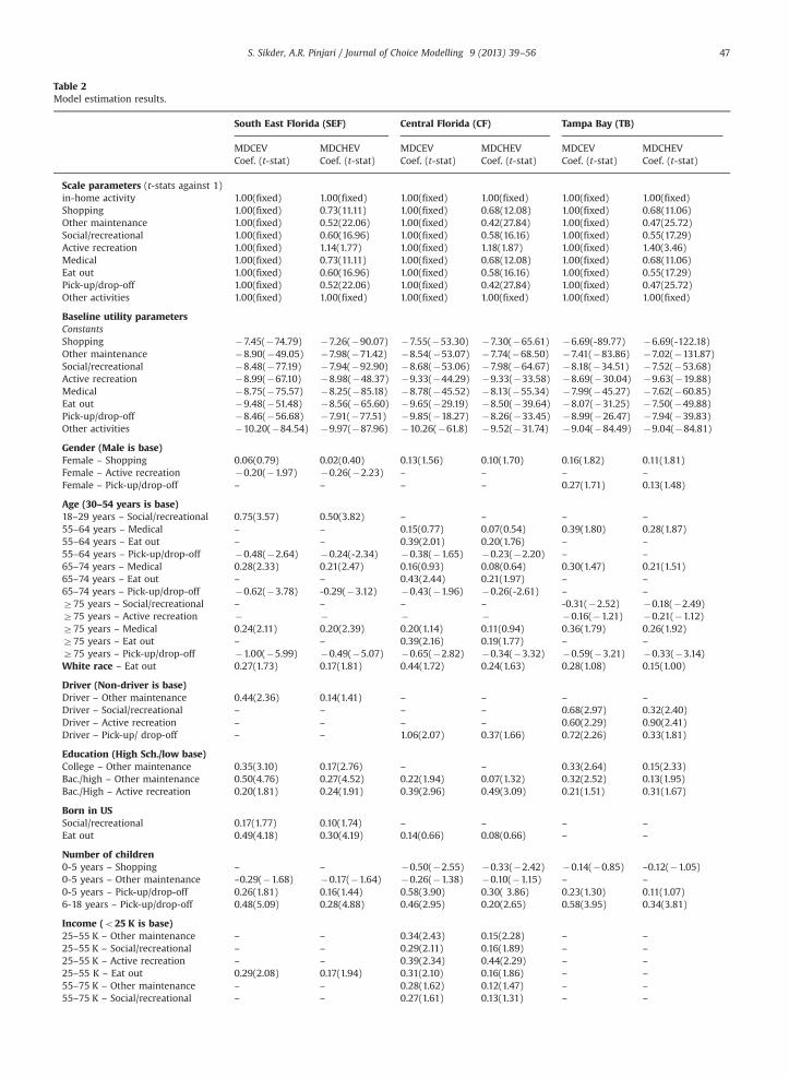
Table 2Model estimation results.

South East Florida (SEF) Central Florida (CF) Tampa Bay (TB)

MDCEV MDCHEV MDCEV MDCHEV MDCEV MDCHEVCoef. (t-stat) Coef. (t-stat) Coef. (t-stat) Coef. (t-stat) Coef. (t-stat) Coef. (t-stat)

Scale parameters (t-stats against 1)in-home activity 1.00(fixed) 1.00(fixed) 1.00(fixed) 1.00(fixed) 1.00(fixed) 1.00(fixed)Shopping 1.00(fixed) 0.73(11.11) 1.00(fixed) 0.68(12.08) 1.00(fixed) 0.68(11.06)Other maintenance 1.00(fixed) 0.52(22.06) 1.00(fixed) 0.42(27.84) 1.00(fixed) 0.47(25.72)Social/recreational 1.00(fixed) 0.60(16.96) 1.00(fixed) 0.58(16.16) 1.00(fixed) 0.55(17.29)Active recreation 1.00(fixed) 1.14(1.77) 1.00(fixed) 1.18(1.87) 1.00(fixed) 1.40(3.46)Medical 1.00(fixed) 0.73(11.11) 1.00(fixed) 0.68(12.08) 1.00(fixed) 0.68(11.06)Eat out 1.00(fixed) 0.60(16.96) 1.00(fixed) 0.58(16.16) 1.00(fixed) 0.55(17.29)Pick-up/drop-off 1.00(fixed) 0.52(22.06) 1.00(fixed) 0.42(27.84) 1.00(fixed) 0.47(25.72)Other activities 1.00(fixed) 1.00(fixed) 1.00(fixed) 1.00(fixed) 1.00(fixed) 1.00(fixed)

Baseline utility parametersConstantsShopping �7.45(�74.79) �7.26(�90.07) �7.55(�53.30) �7.30(�65.61) �6.69(-89.77) �6.69(-122.18)Other maintenance �8.90(�49.05) �7.98(�71.42) �8.54(�53.07) �7.74(�68.50) �7.41(�83.86) �7.02(�131.87)Social/recreational �8.48(�77.19) �7.94(�92.90) �8.68(�53.06) �7.98(�64.67) �8.18(�34.51) �7.52(�53.68)Active recreation �8.99(�67.10) �8.98(�48.37) �9.33(�44.29) �9.33(�33.58) �8.69(�30.04) �9.63(�19.88)Medical �8.75(�75.57) �8.25(�85.18) �8.78(�45.52) �8.13(�55.34) �7.99(�45.27) �7.62(�60.85)Eat out �9.48(�51.48) �8.56(�65.60) �9.65(�29.19) �8.50(�39.64) �8.07(�31.25) �7.50(�49.88)Pick-up/drop-off �8.46(�56.68) �7.91(�77.51) �9.85(�18.27) �8.26(�33.45) �8.99(�26.47) �7.94(�39.83)Other activities �10.20(�84.54) �9.97(�87.96) �10.26(�61.8) �9.52(�31.74) �9.04(�84.49) �9.04(�84.81)

Gender (Male is base)Female – Shopping 0.06(0.79) 0.02(0.40) 0.13(1.56) 0.10(1.70) 0.16(1.82) 0.11(1.81)Female – Active recreation �0.20(�1.97) �0.26(�2.23) – – – –

Female – Pick-up/drop-off – – – – 0.27(1.71) 0.13(1.48)

Age (30–54 years is base)18–29 years – Social/recreational 0.75(3.57) 0.50(3.82) – – – –

55–64 years – Medical – – 0.15(0.77) 0.07(0.54) 0.39(1.80) 0.28(1.87)55–64 years – Eat out – – 0.39(2.01) 0.20(1.76) – –

55–64 years – Pick-up/drop-off �0.48(�2.64) �0.24(-2.34) �0.38(�1.65) �0.23(�2.20) – –

65–74 years – Medical 0.28(2.33) 0.21(2.47) 0.16(0.93) 0.08(0.64) 0.30(1.47) 0.21(1.51)65–74 years – Eat out – – 0.43(2.44) 0.21(1.97) – –

65–74 years – Pick-up/drop-off �0.62(�3.78) -0.29(�3.12) �0.43(�1.96) �0.26(-2.61) – –

Z75 years – Social/recreational – – – – -0.31(�2.52) �0.18(�2.49)Z75 years – Active recreation � � � � �0.16(�1.21) �0.21(�1.12)Z75 years – Medical 0.24(2.11) 0.20(2.39) 0.20(1.14) 0.11(0.94) 0.36(1.79) 0.26(1.92)Z75 years – Eat out – – 0.39(2.16) 0.19(1.77) – –

Z75 years – Pick-up/drop-off �1.00(�5.99) �0.49(�5.07) �0.65(�2.82) �0.34(�3.32) �0.59(�3.21) �0.33(�3.14)White race – Eat out 0.27(1.73) 0.17(1.81) 0.44(1.72) 0.24(1.63) 0.28(1.08) 0.15(1.00)

Driver (Non-driver is base)Driver – Other maintenance 0.44(2.36) 0.14(1.41) – – – –

Driver – Social/recreational – – – – 0.68(2.97) 0.32(2.40)Driver – Active recreation – – – – 0.60(2.29) 0.90(2.41)Driver – Pick-up/ drop-off – – 1.06(2.07) 0.37(1.66) 0.72(2.26) 0.33(1.81)

Education (High Sch./low base)College – Other maintenance 0.35(3.10) 0.17(2.76) – – 0.33(2.64) 0.15(2.33)Bac./high – Other maintenance 0.50(4.76) 0.27(4.52) 0.22(1.94) 0.07(1.32) 0.32(2.52) 0.13(1.95)Bac./High – Active recreation 0.20(1.81) 0.24(1.91) 0.39(2.96) 0.49(3.09) 0.21(1.51) 0.31(1.67)

Born in USSocial/recreational 0.17(1.77) 0.10(1.74) – – – –

Eat out 0.49(4.18) 0.30(4.19) 0.14(0.66) 0.08(0.66) – –

Number of children0-5 years – Shopping – – �0.50(�2.55) �0.33(�2.42) �0.14(�0.85) –0.12(�1.05)0-5 years – Other maintenance –0.29(�1.68) �0.17(�1.64) �0.26(�1.38) �0.10(�1.15) – –

0-5 years – Pick-up/drop-off 0.26(1.81) 0.16(1.44) 0.58(3.90) 0.30( 3.86) 0.23(1.30) 0.11(1.07)6-18 years – Pick-up/drop-off 0.48(5.09) 0.28(4.88) 0.46(2.95) 0.20(2.65) 0.58(3.95) 0.34(3.81)

Income (o25 K is base)25–55 K – Other maintenance – – 0.34(2.43) 0.15(2.28) – –

25–55 K – Social/recreational – – 0.29(2.11) 0.16(1.89) – –

25–55 K – Active recreation – – 0.39(2.34) 0.44(2.29) – –

25–55 K – Eat out 0.29(2.08) 0.17(1.94) 0.31(2.10) 0.16(1.86) – –

55–75 K – Other maintenance – – 0.28(1.62) 0.12(1.47) – –

55–75 K – Social/recreational – – 0.27(1.61) 0.13(1.31) – –


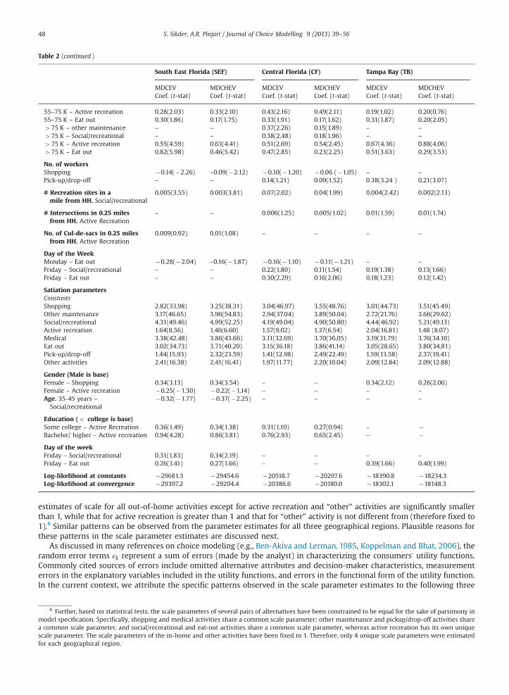
Table 2 (continued )

South East Florida (SEF) Central Florida (CF) Tampa Bay (TB)

MDCEV MDCHEV MDCEV MDCHEV MDCEV MDCHEVCoef. (t-stat) Coef. (t-stat) Coef. (t-stat) Coef. (t-stat) Coef. (t-stat) Coef. (t-stat)

55–75 K – Active recreation 0.28(2.03) 0.33(2.10) 0.43(2.16) 0.49(2.11) 0.19(1.02) 0.20(0.76)55–75 K – Eat out 0.30(1.86) 0.17(1.75) 0.33(1.91) 0.17(1.62) 0.31(1.87) 0.20(2.05)475 K – other maintenance – – 0.37(2.26) 0.15(1.89) – –

475 K – Social/recreational – – 0.38(2.48) 0.18(1.96) – –

475 K – Active recreation 0.55(4.59) 0.63(4.41) 0.51(2.69) 0.54(2.45) 0.67(4.36) 0.88(4.06)475 K – Eat out 0.82(5.98) 0.46(5.42) 0.47(2.85) 0.23(2.25) 0.51(3.63) 0.29(3.53)

No. of workersShopping �0.14(�2.26) –0.09(�2.12) �0.10(�1.20) �0.06 (�1.05) – –

Pick-up/drop-off – – 0.14(1.21) 0.09(1.52) 0.38(3.24 ) 0.21(3.07)

# Recreation sites in amile from HH. Social/recreational

0.005(3.55) 0.003(3.81) 0.07(2.02) 0.04(1.99) 0.004(2.42) 0.002(2.13)

# Intersections in 0.25 milesfrom HH. Active Recreation

– – 0.006(1.25) 0.005(1.02) 0.01(1.59) 0.01(1.74)

No. of Cul-de-sacs in 0.25 milesfrom HH. Active Recreation

0.009(0.92) 0.01(1.08) – – – –

Day of the WeekMonday – Eat out �0.28(�2.04) –0.16(�1.87) �0.16(�1.10) �0.11(�1.21) – –

Friday – Social/recreational – – 0.22(1.80) 0.11(1.54) 0.19(1.38) 0.13(1.66)Friday – Eat out – – 0.30(2.29) 0.16(2.06) 0.18(1.23) 0.12(1.42)

Satiation parametersConstantsShopping 2.82(33.98) 3.25(38.31) 3.04(46.97) 3.55(48.76) 3.01(44.73) 3.51(45.49)Other maintenance 3.17(46.65) 3.96(54.83) 2.94(37.04) 3.89(50.04) 2.72(21.76) 3.66(29.62)Social/recreational 4.31(49.46) 4.99(52.25) 4.19(49.04) 4.90(50.80) 4.44(46.92) 5.21(49.13)Active recreation 1.64(8.56) 1.46(6.60) 1.57(9.02) 1.37(6.54) 2.04(16.81) 1.48 (8.07)Medical 3.38(42.48) 3.86(43.66) 3.11(32.69) 3.70(36.05) 3.19(31.79) 3.76(34.10)Eat out 3.02(34.73) 3.71(40.20) 3.15(36.18) 3.86(41.14) 3.05(28.65) 3.80(34.81)Pick-up/drop-off 1.44(15.93) 2.32(23.59) 1.41(12.98) 2.49(22.49) 1.59(13.58) 2.37(19.41)Other activities 2.41(16.38) 2.41(16.41) 1.97(11.77) 2.20(10.04) 2.09(12.84) 2.09(12.88)

Gender (Male is base)Female – Shopping 0.34(3.13) 0.34(3.54) – – 0.34(2.12) 0.26(2.06)Female – Active recreation �0.25(�1.30) �0.22(�1.14) – – – –

Age. 35-45 years –

Social/recreational�0.32(�1.77) �0.37(�2.25) – – – –

Education (o college is base)Some college – Active Recreation 0.36(1.49) 0.34(1.38) 0.31(1.10) 0.27(0.94) – �Bachelor/ higher – Active recreation 0.94(4.28) 0.86(3.81) 0.76(2.93) 0.65(2.45) – �Day of the weekFriday – Social/recreational 0.31(1.83) 0.34(2.19) – – – –

Friday – Eat out 0.26(1.41) 0.27(1.66) – – 0.39(1.66) 0.40(1.99)

Log-likelihood at constants �29681.3 �29454.6 �20518.7 �20297.6 �18390.8 �18234.3Log-likelihood at convergence �29397.2 �29204.4 �20386.6 �20180.0 �18302.1 �18148.3


estimates of scale for all out-of-home activities except for active recreation and “other” activities are significantly smallerthan 1, while that for active recreation is greater than 1 and that for “other” activity is not different from (therefore fixed to1).8 Similar patterns can be observed from the parameter estimates for all three geographical regions. Plausible reasons forthese patterns in the scale parameter estimates are discussed next.

As discussed in many references on choice modeling (e.g., Ben-Akiva and Lerman, 1985, Koppelman and Bhat, 2006), therandom error terms εk represent a sum of errors (made by the analyst) in characterizing the consumers0 utility functions.Commonly cited sources of errors include omitted alternative attributes and decision-maker characteristics, measurementerrors in the explanatory variables included in the utility functions, and errors in the functional form of the utility function.In the current context, we attribute the specific patterns observed in the scale parameter estimates to the following three

8 Further, based on statistical tests, the scale parameters of several pairs of alternatives have been constrained to be equal for the sake of parsimony inmodel specification. Specifically, shopping and medical activities share a common scale parameter; other maintenance and pickup/drop-off activities sharea common scale parameter, and social/recreational and eat-out activities share a common scale parameter, whereas active recreation has its own uniquescale parameter. The scale parameters of the in-home and other activities have been fixed to 1. Therefore, only 4 unique scale parameters were estimatedfor each geographical region.


major sources of unobserved variation. First, recall from Section 3 that each activity category (i.e., choice alternatives) usedin the model specification is an aggregation of many finely categorized activity types. The influence of explanatory variablesincluded in the utility function of an aggregate activity category can potentially vary by each disaggregate activity type inthat category. Such variation resulting from aggregation of choice alternatives is unobservable and manifests in the form ofadditional variance of random error terms (Daly, 1982). Among the nine activity categories considered in the currentempirical context, the in-home activity is an aggregation of a wider variety of finer activities when compared to out-of-home activities. Recall that the in-home activity category combines all activities other than out-of-home activities into acomposite outside good. This is one reason why the stochastic component of in-home activity has greater variance comparedto most out-of-home activity categories. Second, note from Table 2 that the utility specifications for all activities except thein-home and “other” activity categories include explanatory variables. While the in-home activity category was treated as areference alternative in the specification for identification purposes, no explanatory variable turned out to be significant inthe utility function for the “other” activity category, presumably due to the arbitrary nature of the “other” activity category.Besides, similar to the in-home activity category, the “other” activity category combines all out-of-home activities other thanthose of interest into a single composite category. Thus, the final empirical specification of the deterministic utilitycomponents views in-home and “other” activities as similar (except the alternative-specific constant for “other” activity).This is perhaps a reason why the scale parameter for the “other” activity is not different from the in-home activity. Third, inthe context of discrete-continuous choice modeling, measurement errors in the continuous dependent variables canpotentially be significant. This is unlike traditional discrete choice models, where there might not be significant errors independent variables (because it is easier to elicit information on the discrete choice decisions made by the consumers thanto measure the continuous quantity decisions). In the current empirical application, recall from Section 3 that timeallocation to the active recreational activity might be associated with substantial measurement errors leading to greaterunobservable variation. This may be a reason why the estimated scale parameter for the active recreational activity isgreater than 1.

In summary, the MDCHEV model estimates reveal the presence of substantial heteroscedasticity in the random utilitycomponents of choice alternatives and point to different sources of unobservable variation.

4.2.2. Baseline utility and satiation parametersAll the parameter estimates in baseline utility and satiation functions have intuitive interpretations and identical signs in

both the MDCEV and MDCHEV models for all three regions. The substantive interpretations are not a focus of this paper.Therefore only the influence of incorporating heteroscedasticity on parameter estimates is discussed. Specifically, for all out-of-home activities, except active recreation, the magnitude of baseline utility parameter estimates in the MDCHEV model isslightly smaller than that in the MDCEV model. For active recreation, however, the baseline utility parameter estimates fromthe MDCHEV model are of greater magnitude than those from MDCEV. This pattern can be attributed to the differences inscale parameters between the MDCEV and MDCHEV models. Specifically, the baseline parameter estimates in the MDCEVmodel are confounded with the unknown scale parameters (which are simply assumed to be equal to 1). But the MDCHEVmodel helps in disentangling the baseline parameter estimates from the scale difference between the out-of-home and in-home activities. As a result, all activities with smaller (greater) scale parameters in the MDCHEV model than those in theMDCEV model have smaller (larger) magnitudes for baseline parameter estimates in the former model.

In the context of satiation functions, the parameter estimates of the MDCHEV model are greater (in magnitude) for allout-of-home activities that have a tighter distribution of the random utility component (i.e., smaller scale parameter) thanthat in the MDCEV model. For active recreation activity, the satiation function parameter estimates of the MDCHEV modelare smaller in magnitude than those from the MDCEV model.

Since the true parameter values are unknown, it is difficult to assert which model provides better/less-biased parameterestimates. However, note from the log-likelihood measures for all three geographical regions (last two rows of the table)that the MDCHEV model yields a significantly better fit to the estimation data than the MDCEV model. For example, thelikelihood ratio test statistic between the two models for the South East Florida region is 385.12, which is larger than thechi-squared statistic with four degrees of freedom at any reasonable level of significance. This suggests that ignoringheteroscedasticity (i.e., estimating an MDCEV model) can potentially lead to biased parameter estimates in both baselinemarginal utility and satiation functions and inferior model-fit.

4.3. In-sample prediction performance

All prediction exercises in this paper were performed using the forecasting algorithm proposed by Pinjari and Bhat(2011). In this subsection, we first provide a brief discussion of this forecasting algorithm and then compare the in-sampleprediction performance of the MDCEV and MDCHEV models.

Given the observed characteristics of an individual (e.g.,zk), the available time budget, the estimated parameters, and thesimulated error draws (εk), the forecasting algorithm first identifies the number of chosen alternatives, and then computesthe optimal time allocation to each of the chosen alternatives. In the first step, the price-normalized baseline utility values(ψk=pk) are computed for all choice alternatives. Next, the alternatives are sorted in the descending order of their price-normalized baseline utility values, with the outside good in the first place in this sorted arrangement. Subsequently, thenumber of chosen alternatives is determined. This begins with an assumption that only the first alternative in the above


sorted arrangement is chosen. Based on this assumption, an estimate of the Lagrange multiplier (λ) of the utilitymaximization problem is computed. To check if the next alternative (with the next highest price-normalized baselineutility) is also chosen, the Lagrange multiplier estimated in the previous step is compared with the price-normalizedbaseline utility of the alternative. If the estimated Lagrange multiplier is greater than the price-normalized baseline utility ofthe next alternative, the optimal time allocations to the previously assumed chosen alternatives are calculated and thealgorithm stops. If not, the next alternative is also added to the set of chosen alternatives, and a new estimate of theLagrange multiplier is computed and compared with the next highest price-normalized baseline utility. This procedure isrepeated until the exact number of chosen alternatives is determined. Once the number of chosen alternative is determined,the optimal time allocations are computed using price-normalized baseline utility and satiation parameters of the chosenalternatives and the available time budget.

In this paper, for all prediction exercises, the above-described forecasting procedure was conducted for 100 sets of quasi-Monte Carlo random draws (specifically Halton draws) for each individual in the data to adequately cover the distributionsof the random error terms. The only difference between the MDCEV and the MDCHEV forecasting procedures is that thesimulated error draws come from the IID extreme value distribution for the MDCEV model while they come from theheteroscedastic extreme value (HEV) distribution for the MDCHEV model.

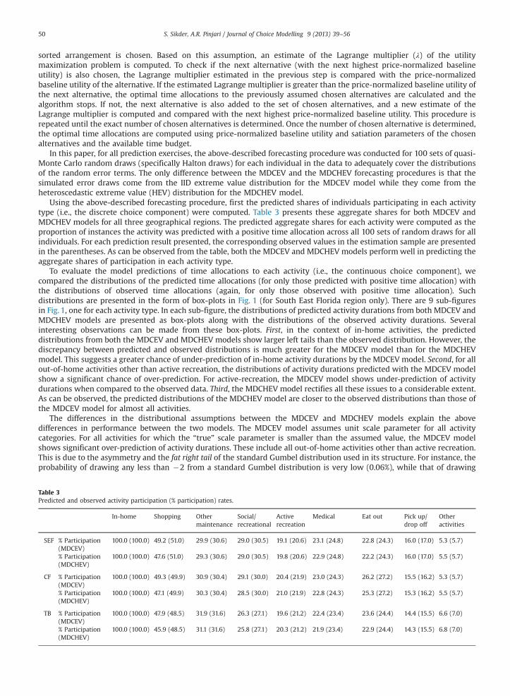
Using the above-described forecasting procedure, first the predicted shares of individuals participating in each activitytype (i.e., the discrete choice component) were computed. Table 3 presents these aggregate shares for both MDCEV andMDCHEV models for all three geographical regions. The predicted aggregate shares for each activity were computed as theproportion of instances the activity was predicted with a positive time allocation across all 100 sets of random draws for allindividuals. For each prediction result presented, the corresponding observed values in the estimation sample are presentedin the parentheses. As can be observed from the table, both the MDCEV and MDCHEV models performwell in predicting theaggregate shares of participation in each activity type.

To evaluate the model predictions of time allocations to each activity (i.e., the continuous choice component), wecompared the distributions of the predicted time allocations (for only those predicted with positive time allocation) withthe distributions of observed time allocations (again, for only those observed with positive time allocation). Suchdistributions are presented in the form of box-plots in Fig. 1 (for South East Florida region only). There are 9 sub-figuresin Fig. 1, one for each activity type. In each sub-figure, the distributions of predicted activity durations from both MDCEV andMDCHEV models are presented as box-plots along with the distributions of the observed activity durations. Severalinteresting observations can be made from these box-plots. First, in the context of in-home activities, the predicteddistributions from both the MDCEV and MDCHEV models show larger left tails than the observed distribution. However, thediscrepancy between predicted and observed distributions is much greater for the MDCEV model than for the MDCHEVmodel. This suggests a greater chance of under-prediction of in-home activity durations by the MDCEV model. Second, for allout-of-home activities other than active recreation, the distributions of activity durations predicted with the MDCEV modelshow a significant chance of over-prediction. For active-recreation, the MDCEV model shows under-prediction of activitydurations when compared to the observed data. Third, the MDCHEV model rectifies all these issues to a considerable extent.As can be observed, the predicted distributions of the MDCHEV model are closer to the observed distributions than those ofthe MDCEV model for almost all activities.

The differences in the distributional assumptions between the MDCEV and MDCHEV models explain the abovedifferences in performance between the two models. The MDCEV model assumes unit scale parameter for all activitycategories. For all activities for which the “true” scale parameter is smaller than the assumed value, the MDCEV modelshows significant over-prediction of activity durations. These include all out-of-home activities other than active recreation.This is due to the asymmetry and the fat right tail of the standard Gumbel distribution used in its structure. For instance, theprobability of drawing any less than �2 from a standard Gumbel distribution is very low (0.06%), while that of drawing

Table 3Predicted and observed activity participation (% participation) rates.

In-home Shopping Othermaintenance

Social/recreational

Activerecreation

Medical Eat out Pick up/drop off

Otheractivities

SEF % Participation(MDCEV)

100.0 (100.0) 49.2 (51.0) 29.9 (30.6) 29.0 (30.5) 19.1 (20.6) 23.1 (24.8) 22.8 (24.3) 16.0 (17.0) 5.3 (5.7)

% Participation(MDCHEV)

100.0 (100.0) 47.6 (51.0) 29.3 (30.6) 29.0 (30.5) 19.8 (20.6) 22.9 (24.8) 22.2 (24.3) 16.0 (17.0) 5.5 (5.7)

CF % Participation(MDCEV)

100.0 (100.0) 49.3 (49.9) 30.9 (30.4) 29.1 (30.0) 20.4 (21.9) 23.0 (24.3) 26.2 (27.2) 15.5 (16.2) 5.3 (5.7)


100.0 (100.0) 47.1 (49.9) 30.3 (30.4) 28.5 (30.0) 21.0 (21.9) 22.8 (24.3) 25.3 (27.2) 15.3 (16.2) 5.5 (5.7)

TB % Participation(MDCEV)

100.0 (100.0) 47.9 (48.5) 31.9 (31.6) 26.3 (27.1) 19.6 (21.2) 22.4 (23.4) 23.6 (24.4) 14.4 (15.5) 6.6 (7.0)


100.0 (100.0) 45.9 (48.5) 31.1 (31.6) 25.8 (27.1) 20.3 (21.2) 21.9 (23.4) 22.9 (24.4) 14.3 (15.5) 6.8 (7.0)

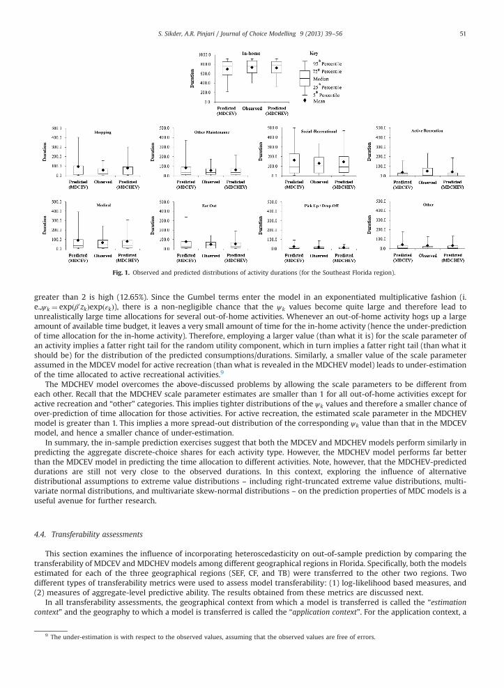
Fig. 1. Observed and predicted distributions of activity durations (for the Southeast Florida region).


greater than 2 is high (12.65%). Since the Gumbel terms enter the model in an exponentiated multiplicative fashion (i.e.,ψk ¼ expðβ0zkÞexpðεkÞ), there is a non-negligible chance that the ψk values become quite large and therefore lead tounrealistically large time allocations for several out-of-home activities. Whenever an out-of-home activity hogs up a largeamount of available time budget, it leaves a very small amount of time for the in-home activity (hence the under-predictionof time allocation for the in-home activity). Therefore, employing a larger value (than what it is) for the scale parameter ofan activity implies a fatter right tail for the random utility component, which in turn implies a fatter right tail (than what itshould be) for the distribution of the predicted consumptions/durations. Similarly, a smaller value of the scale parameterassumed in the MDCEV model for active recreation (than what is revealed in the MDCHEV model) leads to under-estimationof the time allocated to active recreational activities.9

The MDCHEV model overcomes the above-discussed problems by allowing the scale parameters to be different fromeach other. Recall that the MDCHEV scale parameter estimates are smaller than 1 for all out-of-home activities except foractive recreation and “other” categories. This implies tighter distributions of the ψk values and therefore a smaller chance ofover-prediction of time allocation for those activities. For active recreation, the estimated scale parameter in the MDCHEVmodel is greater than 1. This implies a more spread-out distribution of the corresponding ψk value than that in the MDCEVmodel, and hence a smaller chance of under-estimation.

In summary, the in-sample prediction exercises suggest that both the MDCEV and MDCHEV models perform similarly inpredicting the aggregate discrete-choice shares for each activity type. However, the MDCHEV model performs far betterthan the MDCEV model in predicting the time allocation to different activities. Note, however, that the MDCHEV-predicteddurations are still not very close to the observed durations. In this context, exploring the influence of alternativedistributional assumptions to extreme value distributions – including right-truncated extreme value distributions, multi-variate normal distributions, and multivariate skew-normal distributions – on the prediction properties of MDC models is auseful avenue for further research.

4.4. Transferability assessments

This section examines the influence of incorporating heteroscedasticity on out-of-sample prediction by comparing thetransferability of MDCEV and MDCHEV models among different geographical regions in Florida. Specifically, both the modelsestimated for each of the three geographical regions (SEF, CF, and TB) were transferred to the other two regions. Twodifferent types of transferability metrics were used to assess model transferability: (1) log-likelihood based measures, and(2) measures of aggregate-level predictive ability. The results obtained from these metrics are discussed next.

In all transferability assessments, the geographical context from which a model is transferred is called the “estimationcontext” and the geography to which a model is transferred is called the “application context”. For the application context, a

9 The under-estimation is with respect to the observed values, assuming that the observed values are free of errors.


model estimated using data from the same geography is called the “locally estimated model” and a model transferred from adifferent geography is called the “transferred model”.

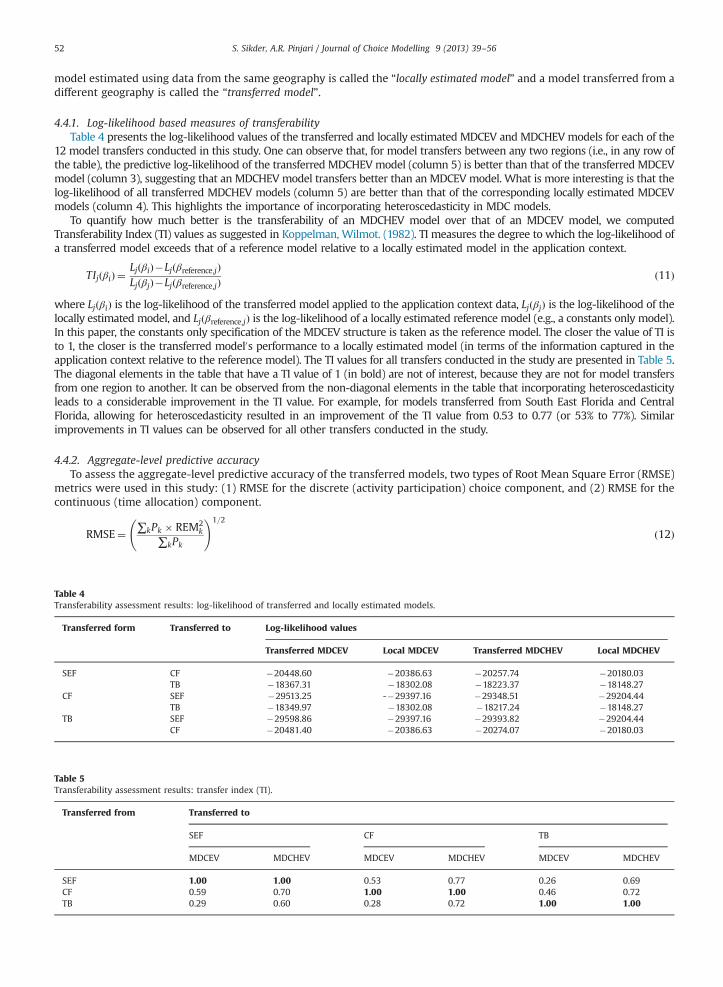
4.4.1. Log-likelihood based measures of transferabilityTable 4 presents the log-likelihood values of the transferred and locally estimated MDCEV and MDCHEV models for each of the

12 model transfers conducted in this study. One can observe that, for model transfers between any two regions (i.e., in any row ofthe table), the predictive log-likelihood of the transferred MDCHEVmodel (column 5) is better than that of the transferred MDCEVmodel (column 3), suggesting that an MDCHEV model transfers better than an MDCEV model. What is more interesting is that thelog-likelihood of all transferred MDCHEV models (column 5) are better than that of the corresponding locally estimated MDCEVmodels (column 4). This highlights the importance of incorporating heteroscedasticity in MDC models.

To quantify how much better is the transferability of an MDCHEV model over that of an MDCEV model, we computedTransferability Index (TI) values as suggested in Koppelman, Wilmot. (1982). TI measures the degree to which the log-likelihood ofa transferred model exceeds that of a reference model relative to a locally estimated model in the application context.

TIjðβiÞ ¼LjðβiÞ�Ljðβreference;jÞLjðβjÞ�Ljðβreference;jÞ

ð11Þ

where LjðβiÞ is the log-likelihood of the transferred model applied to the application context data, LjðβjÞ is the log-likelihood of thelocally estimated model, and Ljðβreference;jÞ is the log-likelihood of a locally estimated reference model (e.g., a constants only model).In this paper, the constants only specification of the MDCEV structure is taken as the reference model. The closer the value of TI isto 1, the closer is the transferred model0s performance to a locally estimated model (in terms of the information captured in theapplication context relative to the reference model). The TI values for all transfers conducted in the study are presented in Table 5.The diagonal elements in the table that have a TI value of 1 (in bold) are not of interest, because they are not for model transfersfrom one region to another. It can be observed from the non-diagonal elements in the table that incorporating heteroscedasticityleads to a considerable improvement in the TI value. For example, for models transferred from South East Florida and CentralFlorida, allowing for heteroscedasticity resulted in an improvement of the TI value from 0.53 to 0.77 (or 53% to 77%). Similarimprovements in TI values can be observed for all other transfers conducted in the study.

4.4.2. Aggregate-level predictive accuracyTo assess the aggregate-level predictive accuracy of the transferred models, two types of Root Mean Square Error (RMSE)

metrics were used in this study: (1) RMSE for the discrete (activity participation) choice component, and (2) RMSE for thecontinuous (time allocation) component.

RMSE¼ ∑kPk � REM2k

∑kPk

!1=2

ð12Þ

Table 4Transferability assessment results: log-likelihood of transferred and locally estimated models.

Transferred form Transferred to Log-likelihood values

Transferred MDCEV Local MDCEV Transferred MDCHEV Local MDCHEV

SEF CF �20448.60 �20386.63 �20257.74 �20180.03TB �18367.31 �18302.08 �18223.37 �18148.27

CF SEF �29513.25 -�29397.16 �29348.51 �29204.44TB �18349.97 �18302.08 �18217.24 �18148.27

TB SEF �29598.86 �29397.16 �29393.82 �29204.44CF �20481.40 �20386.63 �20274.07 �20180.03

Table 5Transferability assessment results: transfer index (TI).

Transferred from Transferred to

SEF CF TB

MDCEV MDCHEV MDCEV MDCHEV MDCEV MDCHEV

SEF 1.00 1.00 0.53 0.77 0.26 0.69CF 0.59 0.70 1.00 1.00 0.46 0.72TB 0.29 0.60 0.28 0.72 1.00 1.00


where Pk and Ok are the aggregate predicted and observed shares for activity type k, respectively (or durations averagedover all individuals who participated in activity type k), and REMk ¼ ðPk�OkÞ=Ok

� �is the percentage error in the prediction

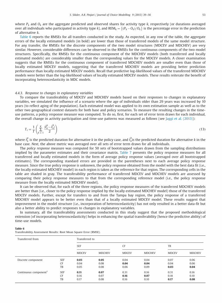
of alternative k.Table 6 reports the RMSEs for all transfers conducted in the study. As expected, in any row of the table, the aggregate

errors of the locally estimated models (in bold) are lower than those of transferred models of the same model structure.For any transfer, the RMSEs for the discrete components of the two model structures (MDCEV and MDCHEV) are verysimilar. However, considerable differences can be observed in the RMSEs for the continuous components of the two modelstructures. Specifically, the RMSEs for the continuous component of the MDCHEV models (both transferred and locallyestimated models) are considerably smaller than the corresponding values for the MDCEV models. A closer examinationsuggests that the RMSEs for the continuous component of transferred MDCHEV models are smaller even than those oflocally estimated MDCEV models, suggesting that the transferred MDCHEV models are providing better predictionperformance than locally estimated MDCEV models. Recall that predictive log-likelihood values of the transferred MDCHEVmodels were better than the log-likelihood values of locally estimated MDCEV models. These results reiterate the benefit ofincorporating heteroscedasticity in MDC models.

4.4.3. Response to changes in explanatory variablesTo compare the transferability of MDCEV and MDCHEV models based on their responses to changes in explanatory

variables, we simulated the influence of a scenario where the age of individuals older than 29 years was increased by 10years (to reflect aging of the population). Each estimated model was applied to its own estimation sample as well as to theother two geographical context datasets for both base and policy scenarios. To measure the resulting changes in the time-use patterns, a policy response measure was computed. To do so, first, for each set of error term draws for each individual,the overall change in activity participation and time-use patterns was measured as follows (see Jaggi et al. (2013)):

Tc ¼1T

∑K

k ¼ 1

jt̂pk� t̂bk j

2

!ð13Þ

where t̂pk is the predicted duration for alternative k in the policy case, and t̂

bkis the predicted duration for alternative k in the

base case. Next, the above metric was averaged over all sets of error term draws for all individuals.The policy response measure was computed for 50 sets of bootstrapped values drawn from the sampling distributions

implied by the parameter estimates and their covariance matrix. Table 7 presents the policy response measures for alltransferred and locally estimated models in the form of average policy response values (averaged over all bootstrappedestimates). The corresponding standard errors are provided in the parentheses next to each average policy responsemeasure. Since the true policy response is unknown, the policy response obtained from the model with the best data fit (i.e.,the locally estimated MDCHEV model) in each region is taken as the reference for that region. The corresponding cells in thetable are shaded in gray. The transferability performance of transferred MDCEV and MDCHEV models are assessed bycomparing their policy response measures to that from the corresponding reference model (i.e., the policy responsemeasure from the locally estimated MDCHEV model).

It can be observed that, for each of the three regions, the policy response measures of the transferred MDCHEV modelsare better than (i.e., closer to the policy response implied by the locally estimated MDCHEV model) those of the transferredMDCEV models. Further, except for transfers to and from the Tampa bay region, the policy response of a transferredMDCHEV model appears to be better even than that of a locally estimated MDCEV model. These results suggest thatimprovement in the model structure (i.e., incorporation of heteroscedasticity) has not only resulted in a better data-fit butalso a better ability to predict responses to changes in explanatory variables.

In summary, all the transferability assessments conducted in this study suggest that the proposed methodologicalextension (of incorporating heteroscedasticity) helps in enhancing the spatial transferability (hence the predictive ability) oftime-use models.

Table 6Transferability Assessment Results: Root Mean Square Error (RMSE).


SEF CF TB


Discrete component SEF 0.03 0.05 0.04 0.04 0.07 0.06CF 0.04 0.08 0.04 0.04 0.04 0.06TB 0.05 0.08 0.06 0.09 0.03 0.04

Continuous component1 SEF 0.11 0.07 0.31 0.16 0.31 0.16CF 0.16 0.07 0.16 0.07 0.18 0.10TB 0.17 0.08 0.16 0.10 0.17 0.08

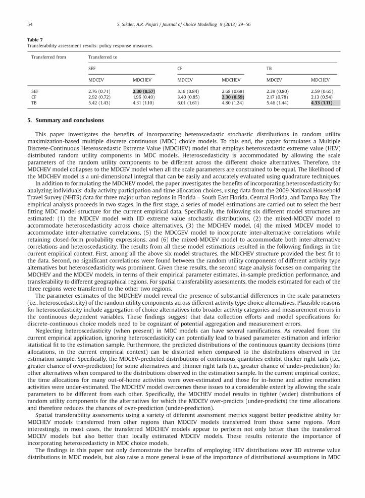
Table 7Transferability assessment results: policy response measures.


SEF CF TB


SEF 2.76 (0.71) 2.30 (0.57) 3.19 (0.84) 2.68 (0.68) 2.39 (0.80) 2.59 (0.65)CF 2.92 (0.72) 1.96 (0.49) 3.40 (0.85) 2.30 (0.59) 2.17 (0.78) 2.13 (0.54)TB 5.42 (1.43) 4.31 (1.10) 6.01 (1.61) 4.80 (1.24) 5.46 (1.44) 4.33 (1.11)


5. Summary and conclusions

This paper investigates the benefits of incorporating heteroscedastic stochastic distributions in random utilitymaximization-based multiple discrete continuous (MDC) choice models. To this end, the paper formulates a MultipleDiscrete-Continuous Heteroscedastic Extreme Value (MDCHEV) model that employs heteroscedastic extreme value (HEV)distributed random utility components in MDC models. Heteroscedasticity is accommodated by allowing the scaleparameters of the random utility components to be different across the different choice alternatives. Therefore, theMDCHEV model collapses to the MDCEV model when all the scale parameters are constrained to be equal. The likelihood ofthe MDCHEV model is a uni-dimensional integral that can be easily and accurately evaluated using quadrature techniques.

In addition to formulating the MDCHEV model, the paper investigates the benefits of incorporating heteroscedasticity foranalyzing individuals0 daily activity participation and time allocation choices, using data from the 2009 National HouseholdTravel Survey (NHTS) data for three major urban regions in Florida – South East Florida, Central Florida, and Tampa Bay. Theempirical analysis proceeds in two stages. In the first stage, a series of model estimations are carried out to select the bestfitting MDC model structure for the current empirical data. Specifically, the following six different model structures areestimated: (1) the MDCEV model with IID extreme value stochastic distributions, (2) the mixed-MDCEV model toaccommodate heteroscedasticity across choice alternatives, (3) the MDCHEV model, (4) the mixed MDCEV model toaccommodate inter-alternative correlations, (5) the MDCGEV model to incorporate inter-alternative correlations whileretaining closed-form probability expressions, and (6) the mixed-MDCEV model to accommodate both inter-alternativecorrelations and heteroscedasticity. The results from all these model estimations resulted in the following findings in thecurrent empirical context. First, among all the above six model structures, the MDCHEV structure provided the best fit tothe data. Second, no significant correlations were found between the random utility components of different activity typealternatives but heteroscedasticity was prominent. Given these results, the second stage analysis focuses on comparing theMDCHEV and the MDCEV models, in terms of their empirical parameter estimates, in-sample prediction performance, andtransferability to different geographical regions. For spatial transferability assessments, the models estimated for each of thethree regions were transferred to the other two regions.

The parameter estimates of the MDCHEV model reveal the presence of substantial differences in the scale parameters(i.e., heteroscedasticity) of the random utility components across different activity type choice alternatives. Plausible reasonsfor heteroscedasticity include aggregation of choice alternatives into broader activity categories and measurement errors inthe continuous dependent variables. These findings suggest that data collection efforts and model specifications fordiscrete-continuous choice models need to be cognizant of potential aggregation and measurement errors.

Neglecting heteroscedasticity (when present) in MDC models can have several ramifications. As revealed from thecurrent empirical application, ignoring heteroscedasticity can potentially lead to biased parameter estimation and inferiorstatistical fit to the estimation sample. Furthermore, the predicted distributions of the continuous quantity decisions (timeallocations, in the current empirical context) can be distorted when compared to the distributions observed in theestimation sample. Specifically, the MDCEV-predicted distributions of continuous quantities exhibit thicker right tails (i.e.,greater chance of over-prediction) for some alternatives and thinner right tails (i.e., greater chance of under-prediction) forother alternatives when compared to the distributions observed in the estimation sample. In the current empirical context,the time allocations for many out-of-home activities were over-estimated and those for in-home and active recreationactivities were under-estimated. The MDCHEV model overcomes these issues to a considerable extent by allowing the scaleparameters to be different from each other. Specifically, the MDCHEV model results in tighter (wider) distributions ofrandom utility components for the alternatives for which the MDCEV over-predicts (under-predicts) the time allocationsand therefore reduces the chances of over-prediction (under-prediction).

Spatial transferability assessments using a variety of different assessment metrics suggest better predictive ability forMDCHEV models transferred from other regions than MDCEV models transferred from those same regions. Moreinterestingly, in most cases, the transferred MDCHEV models appear to perform not only better than the transferredMDCEV models but also better than locally estimated MDCEV models. These results reiterate the importance ofincorporating heteroscedasticty in MDC choice models.

The findings in this paper not only demonstrate the benefits of employing HEV distributions over IID extreme valuedistributions in MDC models, but also raise a more general issue of the importance of distributional assumptions in MDC


models. In this context, exploration of the influence of alternative distributional assumptions – such as multivariateheteroscedastic extreme value and multivariate normal distributions – on the prediction performance of MDC models is apotentially fruitful avenue for further research. Equally important is the need for investigating the relative importance ofinter-alternative correlations vis-à-vis heteroscedasticity in error terms (across alternatives as well as across individuals).Further studies using both simulated data and empirical data to compare the performance of a variety of different modelstructures, including MDCEV, MDCHEV, MDCGEV, mixed-MDCEV, and MDCP models are warranted to address these issues.

Acknowledgments

The second author0s efforts on this paper are dedicated to Mr. Siva Subramanyam Jonnavithula, a transportation engineer,who passed away in July 2013. The authors would like to thank three anonymous reviewers for constructive comments onan earlier manuscript.

References

Ahn, J., Jeong, G., Kim., Y., 2008. A forecast of household ownership and use of alternative fuel vehicles: a multiple discrete-continuous choice approach.Energy Econ 30, 2091–2104.

Ben-Akiva, M.E., Lerman, S.R., 1985. Discrete Choice Analysis: Theory and Application to Predict Travel Demand. MIT press, Cambridge, MA.Bhat, C.R.A., 1995. Heteroscedastic extreme value model of intercity mode choice. Transp. Res. Part B 29 (6), 471–483.Bhat, C.R.A, 2005. Multiple discrete-continuous extreme value model: formulation and application to discretionary time-use decisions. Transp. Res. Part B

39 (.8), 679–707.Bhat, C.R, 2008. The multiple discrete-continuous extreme value (MDCEV) model: role of utility function parameters, identification considerations, and

model extensions. Transp. Res. Part B 42 (3), 274–303.Bhat, C.R., 2011. The maximum approximate composite marginal likelihood (MACML) estimation of multinomial probit-based unordered response choice

models. Transp. Res. Part B 45 (7), 923–939.Bhat, C.R., Sen, S., 2006. Household vehicle type holdings and usage: an application of the multiple discrete-continuous extreme value (MDCEV) model.

Transp. Res. Part B 40 (1), 35–53.Bhat, C.R., Castro, M., Pinjari, A.R., 2013a. Allowing for Non-Additively Separable and Flexible Utility Forms in Multiple Discrete-Continuous Models,

Technical paper. Department of Civil, Architectural and Environmental Engineering, The University of Texas at Austin.Bhat, C.R., Castro, M., Khan., M., 2013b. A New estimation approach for the multiple discrete-continuous probit (MDCP) choice model. Transp. Res. Part B 55,

1–22.Bhat, C.R., Sen, S., Eluru., N., 2009. The impact of demographics, built environment attributes, vehicle characteristics, and gasoline prices on household

vehicle holdings and use. Transp. Res. Part B 43 (1), 1–18.Castro, M., Bhat, C.R., Pendyala, R.M., Jara-Diaz, S.R., 2012. Accommodating multiple constraints in the multiple discrete-continuous extreme value (MDCEV)

choice model. Transp. Res. Part B 46 (6), 729–743.Chikaraishi, M., Zhang, J., Fujiwara, A., Axhausen, K.W., 2010. Exploring variation properties of time use behavior based on a multilevel multiple discrete-

continuous extreme value model. Transp. Res. Part B 2156, 101–110.Daly, A., 1982. Estimating choice models containing attraction variables. Transp. Res. Part B 16 (1), 5–15.Deaton, A.S., Muellbauer., J.N.J., 1980. In: Economics and Consumer BehaviorCambridge University Press, Cambridge.Farooq, B., Miller, E.J., Haider., M., 2013. A multidimensional decisions modeling framework for built space supply. J. Transp. Land Use. (Forthcoming).Frontuto, V., 2011. Residential energy demand: a multiple discrete-continuous extreme value model using Italian expenditure data. European association of

environmental and resource economists, In: Proceedings of the 18th Annual Conference, 29June–2 July, 2011, Rome.Habib, K.M.N., Miller, E.J., 2008. Modeling daily activity program generation considering within-day and day-to-day dynamics in activity-travel behaviour.

Transportation 35 (4), 467–484.Hanemann, W.M.A, 1978. Methodological and Empirical Study of the Recreation Benefits fromWater Quality Improvement (Ph.D. dissertation), Department

of Economics, Harvard University.Jaggi, B., Weis, C., Axhausen., K.W., 2013. Stated response and multiple discrete-continuous choice models: analysis of residuals. J. Choice Model. 6, 44–59.Kaza, N., Towe, C., Ye., X., 2012. A hybrid land conversion model incorporating multiple end uses. Agric. Res. Econ. Rev. 40 (3), 341–359.Kim, J., Allenby, G.M., Rossi, P.E., 2002. Modeling consumer demand for variety. Mark. Sci. 21, 229–250.Koppelman, F.S., Bhat, C.R., 2006. A Self Instructing Course in Mode Choice Modeling: Multinomial and Nested Logit Models, pp. 1–241.Koppelman, F.S., Wilmot., C.G., 1982. Transferability analysis of disaggregate choice models. Transp. Res. Rec. 895, 18–24.Phaneuf, D.J., Kling, C.L., Herriges, J.A., 2000. Estimation and welfare calculations in a generalized corner solution model with an application to recreation

demand. Rev Econ Stat 82 (1), 83–92.Phaneuf, D.J., Smith, V.K., 2005. Recreation Demand Models. In: Mäler, K-G., Vincent, J.R. (Eds.), 2. , Handbook of Environmental Economics, North Holland.Pinjari, A.R., 2011. Generalized extreme value (GEV)-based error structures for multiple discrete-continuous choice models. Transp. Res. Part B 45 (3),

474–489.Pinjari, A.R., Bhat., C.R., 2010. A multiple discrete-continuous nested extreme value (MDCNEV) model: formulation and application to non-worker activity

time-use and timing behavior on weekdays. Transp. Res. Part B 44 (4), 562–583.Pinjari, A.R., Bhat C.R., 2011.Computationally Efficient Forecasting Procedures for Kuhn-Tucker Consumer Demand Model Systems: Application to

Residential Energy Consumption Analysis. Technical Paper, Department of Civil and Environmental Engineering, University of South Florida.Pinjari, A.R., Bhat, C.R., Hensher, D.A., 2009. Residential self-selection effects in an activity-time use behavior model. Transp. Res. Part B 43 (7), 729–748.Pinjari, A.R., Bhat, C.R., Bunch, D.S., 2013. Workshop report: recent advances on multiple discrete-continuous choice models. In: Hess, Stephane, Daly,

Andrew (Eds.), Choice Modelling: The State of the Art and the State of Practice: Selected papers from the Second International Choice ModelingConference, Edward Elgar Publishing, Northampton, USA., pp. 73–90.

Pinjari, A.R., Sivaraman V., 2013. A Discrete-Continuous Choice Model with Perfect and Imperfect Substitutes, Technical Paper. Department of Civil andEnvironmental Engineering, University of South Florida.

Press, W.H., Flannery, B.P., Teukolsky, S.A., Vetterling, W.T., 1986. Numerical Recipes. Cambridge University Press, Cambridge.Satomura, S., Kim, J., Allenby, G., 2011. Multiple constraint choice models with corner and interior solutions. Mark. Sci. 30 (3), 481–490.Sikder, S., Pinjari, A.R., 2013. Spatial transferability of person-level daily activity generation and time-use models: an empirical assessment. Transp. Res. Rec.Spissu, E., Pinjari, A.R., Bhat, C.R., Pendyala, R.M., Axhausen., K.W., 2009. An analysis of weekly out-of-home discretionary activity participation and time-

use behavior. Transportation 36 (5), 483–510.Train, K., 2009. Discrete Choice Methods with Simulation. Cambridge University Press, New York, USA.

http://refhub.elsevier.com/S1755-5345(13)00060-2/sbref1
















































Van Nostrand, C., Sivaraman, V., Pinjari, A.R., 2013. Analysis of annual, long-distance, vacation travel demand in the United States: a multiple discrete-continuous choice framework. Transportation 40 (1), 151–171.

Vasquez-Lavin, F., Hanemann M., 2009. Functional forms in discrete/continuous choice models with general corner solutions. In: Proceedings of the 1stInternational Choice Modeling Conference, Harrogate, March 2009.

von Haefen, R.H., Phaneuf, D.J., 2005. Kuhn-tucker demand system approaches to nonmarket valuation. In: Scarpa, R., Alberini, A.A. (Eds.), Applications ofSimulation Methods in Environmental and Resource Economics, Springer, Netherlands.

von Haefen, R.H., Phaneuf, D.J., Parsons, G.R., 2004. Estimation and welfare analysis with large demand systems. J. Bus. Econ. Stat. 22 (2), 194–205.Wales, T.J., Woodland, A.D., 1983. Estimation of consumer demand systems with binding non-negativity constraints. J. Econom. 21 (3), 263–285.You, D., Garikapati V.M., Konduri K.C., Pendyala R.M., Vovsha P.S., Livshits V., 2013. A multiple discrete-continuous model of activity type choice and time

allocation for home-based non-work tours. In: Proceedings of the 92nd Annual Meeting of the Transportation Research Board, Washington, D.C.Yu, B., Zhang, J., Fujiwara, A., 2012. Representing in-home and out-of-home energy consumption behavior in Beijing. Energy Policy 39 (7), 4168–4177.








Documents

The benefits of allowing heteroscedastic stochastic distributions in multiple discrete-continuous choice models