The Behavior of Mutual Fund Investors

Brad M. Barber*

bmbarber@ucdavis.eduwww.gsm.ucdavis.edu/~bmbarber

Terrance Odeanodean@ucdavis.edu

www.gsm.ucdavis.edu/~odean

Lu Zhengluzheng@umich.edu

First Draft: September 20, 2000Please do not quote without permission from the authors.

Please do not distribute.

* Barber and Odean are at the Graduate School of Management, UC-Davis, Davis, CA 95616-8609. Zheng

is at the School of Business Administration, University of Michigan, Ann Arbor, MI 48109-1234. We aregrateful to the discount brokerage firm that provided us with the data for this study. All errors are ourown.

The Behavior of Mutual Fund Investors

Abstract

We analyze the mutual fund purchase and sale decisions of over 30,000 households with

accounts at a large U.S. discount broker for the six years ending in 1996. We document

three primary results. First, investors buy funds with strong past performance; over half

of all fund purchases occur in funds ranked in the top quintile of past annual returns.

Second, investors sell funds with strong past performance and are reluctant to sell their

losing fund investments; they are twice as likely to sell a winning mutual fund rather than

a losing mutual fund and, thus, nearly 40 percent of fund sales occur in funds ranked in

the top quintile of past annual returns. Third, investors are sensitive to the form in which

fund expenses are charged; though investors are less likely to buy funds with high

transaction fees (e.g., broker commissions or front-end load fees), their purchases are

relatively insensitive to a fund’s operating expense ratio.

We argue that the representative heuristic leads investors to buy past winners, the

disposition effect renders investors reluctant to sell their losers, and framing effects cause

investors to react differently to various forms of fund expenses. Given extant evidence

on the persistence of mutual fund performance, one can reasonably argue that the

purchase of last year’s winning funds is rational. However, we argue that selling winning

fund investments and neglecting a fund’s operating expense ratio when purchasing a fund

is clearly counterproductive.

1

Introduction

For many investors, mutual funds are the investment vehicle of choice. And, this

is increasingly so. From 1991 to 1999 in the U.S., the value of corporate equities held by

mutual funds increased ten-fold, from $309 billion in 1991 to $3.4 trillion in 1999. In

contrast, direct ownership of common stock increased only three-fold during the same

period, from $2.6 trillion to $7.8 trillion. In 1991, 6.4 percent of common stocks were

held indirectly through mutual funds; in 1999, that figure had grown to 18 percent.1 In

1999, nearly half of all U.S. households owned a mutual fund.2 Given the size and

growing importance of mutual fund investors, it is important to gain a better

understanding of their behavior.

In this paper, we attempt to shed light on the behavior of mutual fund investors by

separately analyzing their fund purchase and sale decisions. To do so, we analyze a

unique data set that consists of mutual fund positions and trades for over 30,000

households at a large discount brokerage firm over a six-year period ending in 1996.

We document that fund investors appear to use different decision methods when

deciding what to purchase versus what to sell. When purchasing mutual funds, we argue

that investors use a representativeness heuristic. Investors believe that recent

performance is overly representative of a fund’s future prospects. Thus, investors

predominantly chase past performance. Over half of all purchases occur in funds that

rank in the top quintile of past annual returns. When buying mutual funds, investors act

as though past returns predict future performance.

In contrast, when selling mutual funds, the disposition effect -- the tendency to

hold losers too long and sell winners too soon -- dominates investors’ decisions. When

selling mutual funds, investors do not behave as though past returns predict the future.

1 Flow of Funds Accounts of the United States, 1991-1999, Board of Governors of the Federal Reserve

System, Table L.213, p.82.2 The Investment Company Institute, Mutual Fund Factbook, 2000, reports as of year-end 1999 48.4

million households own mutual funds. In December, 1998, there were roughly 103 million householdsin the U.S.

2

Consistent with this conclusion, we document a positive relation between past

performance and mutual fund sales. Nearly 40 percent of all sales occur in funds that

rank in the top quintile of past annual returns; less than 15 percent of all sales occur in

funds that rank in the bottom quintile. As is the case for many other investments, mutual

fund investors hold their losers and sell their winners.

Our results provide a simple behavioral explanation for the positive, but

asymmetric, relation between net mutual fund flows (purchases less sales) and

performance documented by Ellison and Chevalier (1997) and Sirri and Tufano (1998).

The large net inflows to top-performing funds result from a strong tendency for purchases

to follow past performance. The relatively modest net outflows from the worst-ranked

funds result from reluctance on the part of investors to sell their losing investments.

Mutual fund investors face a dilemma: Is there sufficient persistence in the

performance of successful mutual fund managers to offset the costs of chasing past good

performance? In most professional fields, such as corporate management and law,

practitioners vary in ability. Professionals are evaluated on the basis of past performance.

By analogy, one would expect mutual fund managers to vary in ability and past

performance to be indicative of ability. Yet academic studies find only modest and short-

term persistence in the performance of successful funds.

For the individual investor, there are at least two potential drawbacks to chasing

past performance. First, if one sells a currently held fund to buy a winner, this will

accelerate the recognition of capital gains, thus imposing a tax penalty when done in a

taxable account. Second, top performing funds tend to charge higher operating expenses

and to have higher turnover. High operating expenses and high turnover represent a drag

on a fund’s gross performance, while high turnover further accelerates the recognition of

capital gains.3 Thus, if the fund’s superior gross performance fails to persist, its

performance net of fees, expenses, and taxes is likely to be sub-par.

3

While a particular investor may benefit from chasing performance, investors in

aggregate do not. If investors overestimate their ability to identify superior funds based

on past performance, this will lead to over-investment in active management.

Performance chasing pours more money into funds with high expense ratios and high

turnover. Expense ratios are a drain on investors’ returns; in addition to accelerating

capital gains taxes, high turnover increases trading costs. In aggregate, fees, taxes, and

trading costs represent an unambiguous loss to investors (though a boon to those who

charge these fees). Grossman and Stiglitz (1980) show that in equilibrium rational

investors allocate money to active and passive strategies in proportions that lead to equal

risk-adjusted expected returns to both strategies. Behavioral finance models that

incorporate overconfidence (e.g., Odean (1998a)) provide an even stronger prediction:

active investment strategies will underperform passive investment strategies. Historically,

active management has underperformed passive management, suggesting that too many

resources have been devoted to security research, resulting in sub-optimal returns to

investors.

In addition, by chasing performance, investors create agency conflicts with fund

managers (and more generally fund providers). As noted by several studies (e.g.,

Chevalier and Ellison (1997), Brown, Harlow, and Starks (1996)), the convex

relationship between cash flows and performance may lead managers to focus on

obtaining top performance status rather than focusing on maximizing risk-adjusted

expected returns. And fund providers may start many funds with the intention of

continuing (and advertising) only those with good performance. This practice is likely to

give investors a biased view of how well the average fund is performing and to encourage

further performance chasing.

Selling winning funds, while holding your losers, is clearly an investment

mistake. There is strong empirical evidence that losing mutual funds repeat. Thus,

divesting one’s losing funds would enhance investor returns. And, again, selling winning

3 Furthermore, some mutual fund purchases may incur commissions or fees.

4

rather than losing funds leads to the unnecessary recognition of capital gains, thus

imposing a tax penalty when done in a taxable account.

Finally, we document that the investors react differently to various fund expenses.

Investors are less likely to buy funds that incur salient in-your-face fees, such as a

brokerage commissions or front-end loads. However, their purchases are relatively

insensitive to a fund’s operating expenses. Neglecting a fund’s operating expenses when

purchasing a fund is clearly counterproductive, since it is well documented that mutual

funds with low operating expenses tend to earn higher net returns than funds with high

operating expenses. Though operating expense ratios are disclosed to investors, we

conjecture that many investors overlook these expenses, since the total dollar cost of

these expenses is not disclosed to investors and their effect on the performance of a

particular mutual fund is easily masked by the volatility of a fund’s returns.

The remainder of this paper is organized as follows. We survey related literature

in section I. We describe our data and methods in section II. In section III, we present

results regarding the relation between past fund performance, purchases, and sales. In

section IV, we discuss the welfare implications of these relations. In section V, we

analyze the relation between various fund expenses, purchases, and sales. Concluding

remarks are made in section VI.

I. Background and Related Literature

We argue that mutual fund investors use simple decision heuristics when selecting

mutual funds to purchase or sell. (After presenting our empirical results, we discuss

whether these heuristics affect investor welfare.) When purchasing funds, we posit that

investors use a representativeness heuristic, where recent performance is deemed overly

representative of a fund manager’s true ability. When selling funds, this

representativeness heuristic is more than offset by investors’ reluctance to realize losses

(the disposition effect).

5

A. The Fund Purchase Decision

There are thousands of mutual funds available for purchase. Choosing a mutual

fund for ones investments is a decision fraught with uncertainty. In general, when faced

with uncertain choices, people use heuristics or rules of thumb to make judgments

(Tversky and Kahneman (1974)). Using a representativeness heuristic, people believe

small samples to be overly representative of the population from which they are drawn

(Tversky and Kahneman (1971), Kahneman and Tversky (1972)). Gilovich, Vallone, and

Tversky (1985) document that people systematically underestimate the chance of

observing streaks, such as a run of heads in the flip of an unbiased coin, in a random

sequence. Thus if people do observe streaks of heads or tails when an unbiased coin is

flipped, they are likely to conclude that the coin is biased.

We posit that investors use this representativeness heuristic when buying mutual

funds.4 A fund’s recent performance is viewed as overly representative of a fund

manager’s skill and, thus, of the fund’s future prospects. The abundance of mutual fund

rankings and salient stories about successful fund managers (e.g., Peter Lynch and

Warren Buffet) reinforce the representativeness heuristic. If investors rely on a

representativeness heuristic when selecting mutual funds, they will underestimate the

tendency of fund performance to mean revert and thus anticipate better relative

performance than is realized.

The fact that more money is invested in active than passive funds despite the

superior historical performance of the latter is prima facie evidence that most investors

believe that some mutual fund managers have the ability to consistently beat the market.

Surveys also reveal that investors rely heavily on past performance when evaluating their

fund purchase decisions (Goetzmann and Peles (1997); Capon, Fitzsimons, and Prince

(1996)).

4 Rabin (2000) formerly models this notion by assuming people believe in the “Law of Small Numbers,”

exaggerating the degree to which a small sample resembles the population from which it is drawn. Heconcludes that people may pay for financial advice from “experts” whose expertise is entirely illusory.

6

B. The Fund Sale DecisionThe decision to sell a mutual fund is quite different from the decision to purchase

a fund. Most investors hold few funds. In 1998, the average household held five mutual

funds.5 Thus, unlike purchases where investors have thousands of funds to choose from,

investors have only a handful of funds from which to choose when selling.

Using the representativeness heuristic, investors would view poor fund

performance as overly representative of a manager’s skill and sell losing fund

investments. However, this representativeness heuristic is partially offset by investors’

desire to avoid the recognition of losses or loss aversion. In contrast to the

representativeness heuristic, loss aversion predicts that investors will sell their winning

funds, while holding their losers.

Kahneman and Tversky (1979) argue that people are loss averse: they have an

asymmetric attitude to gains and losses, getting less utility from gaining, say, $100 than

they would lose if they lost $100 (having started $100 wealthier). If investors use the

purchase price of their mutual funds as a reference point, prospect theory predicts that

mutual fund investors would be more likely to sell their winning mutual funds than their

losers. The disposition to sell winners and hold losers has been dubbed the “disposition

effect” (Shefrin and Statman (1985)).

The disposition effect has a large effect on the investors selling decisions for

many asset classes, including individual common stocks (Odean (1998), Grinblatt and

Keloharju (2000)), company stock options (Heath, Huddart, and Lang (1999)), residential

housing (Genesove and Mayer (1999)), and futures (Locke and Mann (1999)).

It is not at all obvious that these findings would extend to mutual funds. On the

one hand, investors may view the decision to sell a mutual fund as an investment decision

like any other. In this “investment” frame, the investor holds responsibility for the

5 The Investment Company Institute, Mutual Fund Factbook, 2000, p.47.

7

performance of the mutual fund and the role of the mutual fund manager is secondary.

Thus, investors using this frame will be reluctant to realize losses (the disposition effect).

On the other hand, investors may view mutual fund managers as agents, who are

responsible for the management of their money. In this “agency” frame, the selling

decision is more like a firing decision: Shall I fire my mutual fund manager for delivering

poor performance? Using this frame, it is easy for the investor to blame an external factor

-- the poor ability of the mutual fund manager -- for the fund's poor performance. Thus,

they will be willing to realize losses (i.e., fire the mutual fund manager).

We suspect that investors use both the investment frame and the agency frame.

Which frame dominates in the selling decisions of mutual fund investors is an empirical

question, which we address in this research. We provide strong evidence that it is the

disposition effect, rather than the agency frame, that determines which funds investors

sell.

II. Data and Methods

A. Mutual Fund Account Data

The primary data set for this research is information from a large discount

brokerage firm on the investments of 78,000 households from January 1991 through

December 19966: 42 percent of the sampled households reside in the western part of the

United States, 19 percent in the East, 24 percent in the South, and 15 percent in the

Midwest. The data set includes all accounts opened by each household at this discount

brokerage firm. This data set has two main advantages over the fund level cash flow data

in many earlier studies: 1) it enables us to separately analyze purchase and redemption

decisions, 2) it discloses the exact timing and amount of money flows so that the cash

flow measures are more reliable than the estimates from TNA and fund returns; the

earlier estimates impose simplified timing assumptions upon cash flows.

6 The month-end position statements for this period allow us to calculate returns for February 1991 through

January 1997. Data on trades are from January 1991 through November 1996.

8

In this research, we focus on the mutual fund investments of households. We

exclude from the current analysis investments in common stocks, American depository

receipts (ADRs), warrants, and options. Of the 78,000 sampled households, 32,199 (41

percent) had positions in mutual funds during at least one month; the remaining accounts

either held cash or investments in securities other than mutual funds. Seventeen percent

of the market value in the accounts was held in mutual funds and 64 percent in individual

common stocks. There were over 3 million trades in all securities. Mutual funds

accounted for 18 percent of all trades; individual common stocks accounted for 64

percent.

Of the 32,199 households with positions in mutual funds, the average held 3.6

mutual funds worth $36,988. Both of these numbers are positively skewed. The median

household held 2 mutual funds worth $12,844 dollars. For these households, the

positions in mutual funds and individual common stocks were roughly equal. Forty-two

percent of the market value in these accounts was held in mutual funds and 39 percent in

individual common stocks. In aggregate, these households held 1,073 mutual funds

worth $1.4 billion in December 1996.

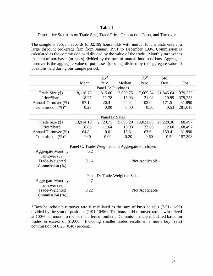
In Table I, we present descriptive information on the trading activity for our

sample. Panel A presents information on purchases, while Panel B contains information

on sales. There were roughly twice as many purchases (379,253) as sales (168,497)

during our sample period, though the average value of funds sold ($13,914) was greater

than the value of funds purchased ($8,119). As a result, the aggregate value of purchases

($3 billion) was 30 percent greater than the aggregate value of sales ($2.3 billion). In

contrast, the 78,000 households that compose our sample bought and sold equal amounts

of individual common stocks ($12 billion each). These patterns are consistent with

overall economic trends during our sample period. According to Federal Reserve Flow

of Funds data, households directly held 49.9 percent of U.S. equities in 1990 and 47.4

percent in 1996. In contrast, the holdings of U.S. equities by mutual funds more than

doubled -- from 6.6 percent in 1990 to 14.5 percent in 1996.

9

For each household, we calculate the purchase turnover rate for mutual fund

holdings as the sum of purchases divided by the sum of monthly positions. We calculate

sales turnover similarly. To reduce the effect of outliers, monthly turnover is winsorized

at 100 percent. For the average household, purchase turnover was 97 percent annually,

while sales turnover was 65 percent. Both turnover rates are positively skewed; for the

median household, purchase turnover was 44 percent, while sales turnover was 16

percent. Aggregate purchase (or sales) turnover is calculated by summing purchases (or

sales) and positions across all accounts and taking the ratio of the two sums. In

aggregate, purchase turnover was 74 percent; sales turnover was 56 percent. Fund

turnover rates are similar to those for individual common stocks. Barber and Odean

(2000) report average, median, and aggregate turnover rates of 75 percent, 31 percent,

and 79 percent, respectively, for individual common stocks held by these households.

With the exception of load and exit fees, mutual fund investors can generally

purchase mutual funds directly from the fund complex at zero transaction costs. When

purchasing mutual funds through a broker, a commission is charged for the purchase or

sale of some funds. Generally fund complexes will pay a fee to the broker to gain status

as a non-transaction fee (NTF) fund. These fees are designated as 12b-1 fees by the fund

complex. In our sample, 76 percent of fund purchases and 49 percent of sales are NTF

funds.

For each trade in excess of $1,000, we calculate the percentage commission as the

commission divided by the value of the trade. The average purchase costs 0.28 percent,

while the average sale costs 0.40 percent. We also calculate the trade-weighted (weighted

by trade size) commissions. These figures can be thought of as the total cost of

conducting the $5.3 billion in fund trades ($3 billion in purchases and $2.3 billion sales).

In aggregate, these investors paid 0.16 percent for purchases and 0.22 percent for sales.

(Loads are transaction costs that investors pay when they trade and are not included in the

calculation here.)

10

For the investor, it is cheaper to trade mutual funds than individual common

stocks. In our sample, the average round-trip cost of trading mutual funds is 0.68

percent, while the average round-trip cost of trading individual common stocks is 4

percent (Barber and Odean, 2000). (The latter cost reflects round-trip commissions of 3

percent and a round-trip bid-ask spread of 1 percent.) In short, the investor who buys or

sells a mutual fund pays a relatively small direct cost for trading.

However, in aggregate, investors pay an indirect cost for their trading. When a

fund investor purchases shares in an open-end mutual fund, the fund manager will invest

the new money in individual common stock. Similarly, when an investor sell shares, the

manager must divest some stock holdings.7 Though the investor pays no commission for

the purchase or sale of the fund share, she is indirectly affected since her purchases and

sales generate trades, and their attendant costs, at the fund level. Edelen (1999)

documents that these trades cost the average fund more than 1 percent annually, while

Chalmers, Edelen, and Kadlac (2000) document fund performance is negatively related to

the level of trading costs. Note that trading costs are born equally by all investors in the

fund, not just those who transact frequently. Thus, long-term buy-and-hold investors

subsidize the trading of fickle fund investors.8

B. Returns DataMonthly mutual fund returns data are from the Center for Research in Security

Prices (CRSP) mutual fund database. Consistent with many prior mutual fund studies,

we restrict our analysis to diversified U.S. equity mutual funds. 9 Thus, we exclude from

7 Edelen (1999) estimates that 70 percent of mutual fund flows generate trade. The remaining 30 percent

are either crossed or generate trading that would have occurred anyway.8 To mitigate this externality for long-term buy-and-hold investors, some mutual funds charge purchase or

redemption fees when investors buy and sell mutual funds. These fees are added to funds assets and aredesigned to offset trading costs generated by fund flows.

9 We select funds based on four sets of criteria. First, we select funds with the following ICDI objectives:aggressive growth, growth and income, long-term growth, or total return (only if they have the followingStrategic Insight’s fund objectives: flexible, growth, or income growth). If ICDI objectives are missing,we select funds with the following Strategic Insight’s fund objectives: aggressive growth, growth &income, growth, income growth, or small company growth. If both ICDI and Strategic Insight’sobjectives are missing, we select funds with the following Weisenberger fund types: AAL, AGG, G, G-I,G-I-S, G-S, G-S-I, GCI, GRI, GRO, I-G, I-G-S, I-S, I-S-G, MCG, SCG, or TR. If all three of the abovecriteria are missing, we select funds described as common stocks according to the policy and objectivecodes.

11

our analyses bond funds, international equity funds, and specialized sector funds. In

addition, we are not able to accurately match to the CRSP mutual fund database 5 percent

of mutual fund trades.10 Our final sample consists of 226,592 mutual fund purchases and

85,731 mutual fund sales.

C. Calculation of Proportion of Gains or Losses Realized (PGR andPLR)To determine whether mutual fund investors sell winners more readily than losers,

it is not sufficient to look at the number of funds sold for gains versus the number sold for

losses. Suppose investors are indifferent to selling winners and losers. Then in an

upward-moving market they will have more winners in their portfolios and will tend to

sell more winners than losers even though they had no preference for doing so. To test

whether investors are disposed to selling winners and holding losers, we must look at the

frequency with which they sell winners and losers relative to their opportunities to sell

each.

By going through each household’s trading records, we construct for each date a

portfolio of funds for which the purchase date and price are known.11 Each day that a

sale takes place in a portfolio of two or more funds, we compare the selling price for each

fund to its average purchase price to determine whether the fund was sold for a gain or a

loss. Each fund that is in that portfolio at the beginning of that day, but is not sold, is

considered to be a paper (unrealized) gain or loss. On days when no sales take place in an

account, no gains or losses (realized or paper) are counted. Realized gains, paper gains,

realized losses, and paper losses are summed over time for each account and across

accounts. Based on these counts, two ratios are calculated:

10 We match funds from the two data sets primarily by matching the series of month-end NAVs. We also

double check by matching CUSIP identifiers and fund names when available.11 Since we are working with monthly returns for mutual funds, we calculate gains and losses by assuming

mutual funds are bought and sold on the last day of the month, rather than the actual trade date. Wefurther assume that distributions are reinvested in the fund that paid them, which is a common practicefor fund investors.

12

.lossesPaper losses Realized

losses Realized (PLR)realized losses of Proportion

;gainsPaper gains Realized

gains Realized (PGR) realized gains of Proportion

+=

+=

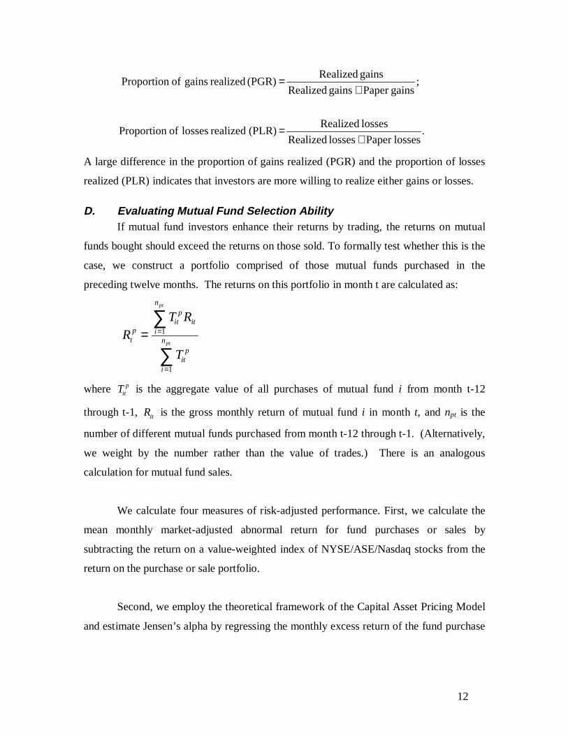
A large difference in the proportion of gains realized (PGR) and the proportion of losses

realized (PLR) indicates that investors are more willing to realize either gains or losses.

D. Evaluating Mutual Fund Selection AbilityIf mutual fund investors enhance their returns by trading, the returns on mutual

funds bought should exceed the returns on those sold. To formally test whether this is the

case, we construct a portfolio comprised of those mutual funds purchased in the

preceding twelve months. The returns on this portfolio in month t are calculated as:

RT R

Ttp

itp

iti

n

itp

i

n

pt

pt= =

=

∑

∑1

1

where Titp is the aggregate value of all purchases of mutual fund i from month t-12

through t-1, Rit is the gross monthly return of mutual fund i in month t, and npt is the

number of different mutual funds purchased from month t-12 through t-1. (Alternatively,

we weight by the number rather than the value of trades.) There is an analogous

calculation for mutual fund sales.

We calculate four measures of risk-adjusted performance. First, we calculate the

mean monthly market-adjusted abnormal return for fund purchases or sales by

subtracting the return on a value-weighted index of NYSE/ASE/Nasdaq stocks from the

return on the purchase or sale portfolio.

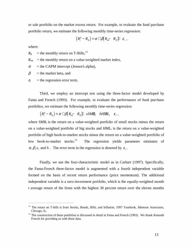
Second, we employ the theoretical framework of the Capital Asset Pricing Model

and estimate Jensen’s alpha by regressing the monthly excess return of the fund purchase

13

or sale portfolio on the market excess return. For example, to evaluate the fund purchase

portfolio return, we estimate the following monthly time-series regression:

R R R Rt ft mt ft tp ,− = + − +3 8 3 8α β ε

where:

Rft = the monthly return on T-Bills,12

Rmt = the monthly return on a value-weighted market index,

α = the CAPM intercept (Jensen’s alpha),

β = the market beta, and

εi = the regression error term.

Third, we employ an intercept test using the three-factor model developed by

Fama and French (1993). For example, to evaluate the performance of fund purchase

portfolios, we estimate the following monthly time-series regression:

R R R R sSMB hHMLt ft mt ft t t tp ,− = + − + + +3 8 3 8α β ε

where SMBt is the return on a value-weighted portfolio of small stocks minus the return

on a value-weighted portfolio of big stocks and HMLt is the return on a value-weighted

portfolio of high book-to-market stocks minus the return on a value-weighted portfolio of

low book-to-market stocks.13 The regression yields parameter estimates of

α β, , ,s h and . The error term in the regression is denoted by ε t .

Finally, we use the four-characteristic model as in Carhart (1997). Specifically,

the Fama-French three-factor model is augmented with a fourth independent variable

formed on the basis of recent return performance (price momentum). The additional

independent variable is a zero-investment portfolio, which is the equally-weighted month

t average return of the firms with the highest 30 percent return over the eleven months

12 The return on T-bills is from Stocks, Bonds, Bills, and Inflation, 1997 Yearbook, Ibbotson Associates,

Chicago, IL.13 The construction of these portfolios is discussed in detail in Fama and French (1993). We thank Kenneth

French for providing us with these data.

14

through month t-2, less the equally-weighted month t average return of the firms with the

lowest 30 percent return over the eleven months through month t-2.

III. Results

A. Proportion of Gains and Losses Realized

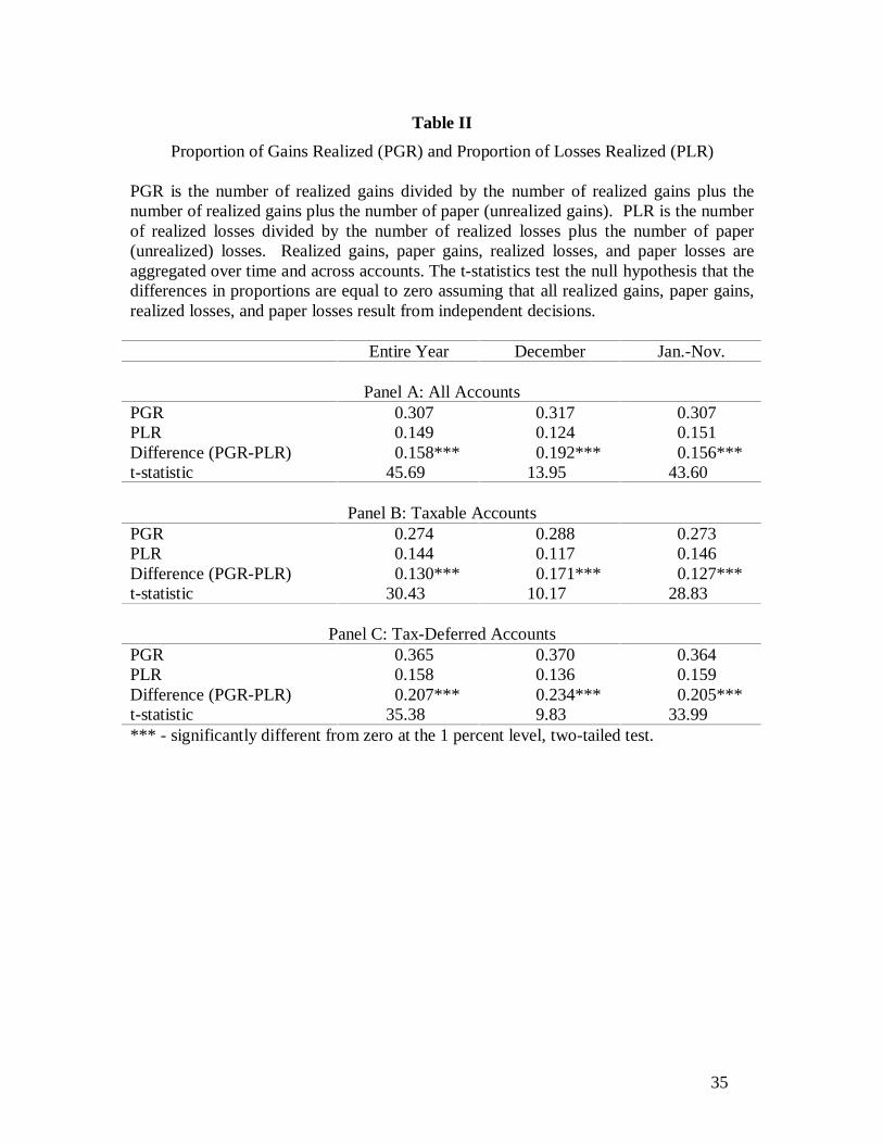
In Table II, panel A, we present the calculation of the proportion of gains realized

(PGR) and the proportion of losses realized (PLR) for all accounts. For this analysis, we

only analyze investors who had a choice to sell a fund for a gain or a fund for a loss.

Thus, investors must have held at least one fund for a gain and one fund for a loss at the

time of a sale to be included in the analysis. (Our results are qualitatively similar if we

relax this requirement.) Consistent with the predictions of the disposition effect,

investors prefer to sell funds for a gain, rather than a loss. The difference between PGR

and PLR is reliably greater than zero, with t-statistics greater than 10. On average,

investors are twice as likely to sell a fund for a gain, rather than a loss.

Are taxes an important consideration in the selling decision of mutual fund

investors? One would expect investors to realize losses -- particularly late in the year --

so that these losses can be used to shelter the realization of capital gains. To analyze this

issue, we calculate PGR and PLR for taxable and tax-deferred accounts (e.g., Keoghs and

401(k) accounts). If taxes are an important determinant of investors’ selling decision, we

would expect losses to be realized at a greater rate in taxable, as opposed to tax-deferred

accounts. We also calculate PGR and PLR for sales made in January through November

versus those made in December. If taxes are an important determinant of investors’

selling decision, we would expect losses to be realized at a greater rate in December, as

opposed to January through November.

The results of this analysis are presented in panels B and C of Table II. In Figure

1, we plot the ratio of PGR to PLR for taxable and tax-deferred accounts. If investors are

equally likely to realize gains and losses (relative to their opportunities realize each), this

ratio would be one. There is, at best, weak evidence that taxes are an important

determinant of investors’ selling decision. The ratio of PGR to PLR is slightly higher for

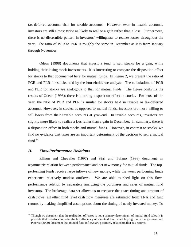
15

tax-deferred accounts than for taxable accounts. However, even in taxable accounts,

investors are still almost twice as likely to realize a gain rather than a loss. Furthermore,

there is no discernible pattern in investors’ willingness to realize losses throughout the

year. The ratio of PGR to PLR is roughly the same in December as it is from January

through November.

Odean (1998) documents that investors tend to sell stocks for a gain, while

holding their losing stock investments. It is interesting to compare the disposition effect

for stocks to that documented here for mutual funds. In Figure 2, we present the ratio of

PGR and PLR for stocks held by the households we analyze. The calculations of PGR

and PLR for stocks are analogous to that for mutual funds. The figure confirms the

results of Odean (1998); there is a strong disposition effect in stocks. For most of the

year, the ratio of PGR and PLR is similar for stocks held in taxable or tax-deferred

accounts. However, in stocks, as opposed to mutual funds, investors are more willing to

sell losers from their taxable accounts at year-end. In taxable accounts, investors are

slightly more likely to realize a loss rather than a gain in December. In summary, there is

a disposition effect in both stocks and mutual funds. However, in contrast to stocks, we

find no evidence that taxes are an important determinant of the decision to sell a mutual

fund.14

B. Flow-Performance Relations

Ellison and Chevalier (1997) and Sirri and Tufano (1998) document an

asymmetric relation between performance and net new money for mutual funds. The top-

performing funds receive large inflows of new money, while the worst performing funds

experience relatively modest outflows. We are able to shed light on this flow-

performance relation by separately analyzing the purchases and sales of mutual fund

investors. The brokerage data set allows us to measure the exact timing and amount of

cash flows; all other fund level cash flow measures are estimated from TNA and fund

returns by making simplified assumptions about the timing of newly invested money. To

14 Though we document that the realization of losses is not a primary determinant of mutual fund sales, it is

possible that investors consider the tax efficiency of a mutual fund when buying funds. Bergstresser andPoterba (2000) document that mutual fund inflows are positively related to after-tax returns.

16

do so, in month t, we partition funds into deciles on the basis of their 12-month return

through month t-1. We then measure the intensity of buying (or selling) in each

performance decile.

We summarize these results in Table III. Columns two and three of the table

present the average fund size and the proportion of all funds in each performance decile.

Small funds appear more often in the extreme deciles, particularly the worst-performing

funds.

Investors chase performance when purchasing funds. Columns four and five of

the table reveal that investors predominantly buy funds with strong past performance; the

top two performance deciles represent roughly one-fifth of all mutual fund investments

(21 percent), but account for over half of all purchases (54 percent). In light of the flow-

performance relations documented by Ellison and Chevalier (1997) and Sirri and Tufano

(1998), these patterns perhaps are not surprising.

What is surprising, is the intensity of selling activity in the top-performing mutual

funds. Consistent with the disposition effect documented in the prior section, the top two

performance deciles account for 38 percent of all sales, while the bottom two account for

merely 14 percent of sales (and 12.5 percent of mutual fund investments).

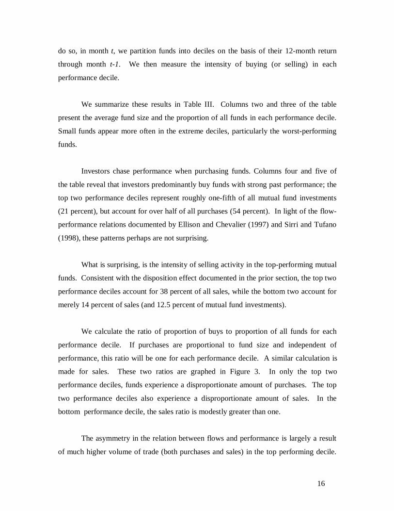
We calculate the ratio of proportion of buys to proportion of all funds for each

performance decile. If purchases are proportional to fund size and independent of

performance, this ratio will be one for each performance decile. A similar calculation is

made for sales. These two ratios are graphed in Figure 3. In only the top two

performance deciles, funds experience a disproportionate amount of purchases. The top

two performance deciles also experience a disproportionate amount of sales. In the

bottom performance decile, the sales ratio is modestly greater than one.

The asymmetry in the relation between flows and performance is largely a result

of much higher volume of trade (both purchases and sales) in the top performing decile.

17

As seen in the last column of Table III, the proportion of all trades that are buys decreases

nearly linearly when one moves from the top performance decile to the bottom

performance decile. For example, the percentage of all trades that are buys is 66 percent

in the top performance decile and 35 percent in the bottom performance decile. Thus, if

trading volume were equal in the two extreme deciles, the relation between flows and

performance would be symmetric; poor performing funds would experience outflows at

roughly the same rate that top performing funds experience inflows. But a

disproportionate amount of fund trades occur in the top performance decile.

The purchase and sale behavior that we document yields a positive, but

asymmetric, relation between mutual fund flows and performance. A strong tendency for

purchases to follow strong past performance yields large net inflows to top-ranked funds.

The reluctance of investors to sell losing funds moderates the outflows of poorly ranked

funds.

IV. Welfare Implications of Investor BehaviorDo the behaviors that we document -- chasing performance and holding losers --

affect investor welfare? To address this issue, we first analyze the performance of the

investors studied here. Neither chasing performance nor holding losers improved the

performance of the investors we study. However, we are well aware that the short

sample period that we study (six years) may yield insufficient power for definitive

conclusions. Thus, we also consider the implications of prior empirical research on

mutual fund performance persistence and the fund selection ability of individual

investors. Ultimately, we can make a strong case that selling winners, while holding

losers, is counterproductive. However, it is ambiguous whether it is prudent to chase

performance when purchasing funds.

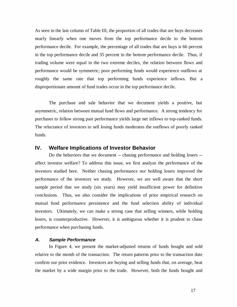
A. Sample PerformanceIn Figure 4, we present the market-adjusted returns of funds bought and sold

relative to the month of the transaction. The return patterns prior to the transaction date

confirm our prior evidence. Investors are buying and selling funds that, on average, beat

the market by a wide margin prior to the trade. However, both the funds bought and

18

those sold fail to beat the market following the trade. Furthermore, the returns on funds

bought are roughly equal to the returns on those sold.

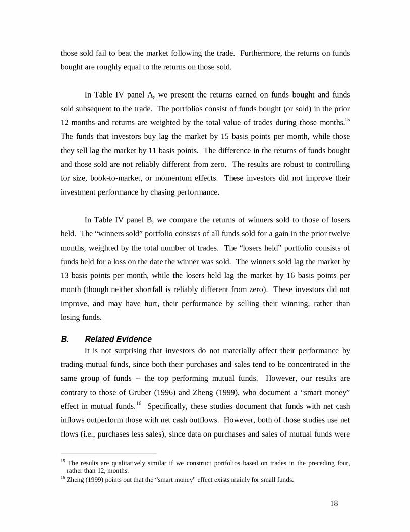
In Table IV panel A, we present the returns earned on funds bought and funds

sold subsequent to the trade. The portfolios consist of funds bought (or sold) in the prior

12 months and returns are weighted by the total value of trades during those months.15

The funds that investors buy lag the market by 15 basis points per month, while those

they sell lag the market by 11 basis points. The difference in the returns of funds bought

and those sold are not reliably different from zero. The results are robust to controlling

for size, book-to-market, or momentum effects. These investors did not improve their

investment performance by chasing performance.

In Table IV panel B, we compare the returns of winners sold to those of losers

held. The “winners sold” portfolio consists of all funds sold for a gain in the prior twelve

months, weighted by the total number of trades. The “losers held” portfolio consists of

funds held for a loss on the date the winner was sold. The winners sold lag the market by

13 basis points per month, while the losers held lag the market by 16 basis points per

month (though neither shortfall is reliably different from zero). These investors did not

improve, and may have hurt, their performance by selling their winning, rather than

losing funds.

B. Related EvidenceIt is not surprising that investors do not materially affect their performance by

trading mutual funds, since both their purchases and sales tend to be concentrated in the

same group of funds -- the top performing mutual funds. However, our results are

contrary to those of Gruber (1996) and Zheng (1999), who document a “smart money”

effect in mutual funds.16 Specifically, these studies document that funds with net cash

inflows outperform those with net cash outflows. However, both of those studies use net

flows (i.e., purchases less sales), since data on purchases and sales of mutual funds were

15 The results are qualitatively similar if we construct portfolios based on trades in the preceding four,

rather than 12, months.16 Zheng (1999) points out that the “smart money” effect exists mainly for small funds.

19

not available to them. Portfolios formed on the basis of net flows obviously distort the

average experience of investors, since the majority of sales take place in the same group

of funds that experience the largest net inflows -- the top performing funds.

Nonetheless, the “smart money” effect of Gruber (1996) and Zheng (1999) is

sufficient to conclude funds purchased by investors earn higher returns than those sold.

Thus, the difference in the results of these studies and our own can be explained either by

a different sample period (ours is much shorter than theirs) or the use of different data

(Gruber and Zheng use aggregate fund flows, while ours are based on trades at a single

discount broker).

Based on auxiliary analyses, we conclude that the difference in our results

emanates mainly from our short sample period, rather than the use of different data.

Specifically, we construct a positive new money portfolio, which consists of funds with

positive net cash flows in the previous quarter (weighted in proportion to the net cash

inflow for the fund). Similarly, we construct a negative new money portfolio.

Regardless of whether we base inflows and outflows solely on the brokerage house data

used in this study or, alternatively, on aggregate flows (as in Zheng (1999)), the cash flow

weighted positive new money portfolio earns monthly returns that are virtually identical

to that earned on the cash flow weighted negative new money portfolio.17 Zheng (1999)

documents that most of the returns earned by these new money portfolios can be

attributed to performance persistence in mutual funds. Thus, the lack of significant results

can likely be attributed to relatively weak fund performance persistence during our

sample period. When we replicate the results of Carhart (1997) for our sample period, the

funds ranked in the top decile based on prior-year performance beat the bottom decile

17 Using the brokerage house data, the positive new money portfolio earned returns that were 1.5 basis

points per month less than the negative new money portfolio (p-value = 0.87). Using aggregate flowdata, the positive new money portfolio earned returns that were 1.1 basis points per month greater thanthe negative new money portfolio (p-value = 0.88). There is some marginal evidence that the equallyweighted positive new money portfolio outperforms the negative one for our sample period when weshift from the brokerage house data to the aggregate flow data. However, we believe that implicationswe get from the cash flow weighted portfolios are more relevant in addressing the welfare question. The“smart money” effect is also stronger when we focus on a subset of smaller funds.

20

funds by 28 basis points per month; this return difference is less than half that reported by

Carhart. We elaborate on the crucial link between fund performance persistence and the

sagacity of investors’ mutual fund purchases and sales in the next section.

C. Is Chasing Performance Rational ?Is it rational for investors to chase performance when purchasing mutual funds?

That depends on the degree to which past fund performance can predict future fund

returns and on the costs associated with chasing performance.

Empirically, there is evidence that past fund performance is useful in predicting

future returns (Hendricks, Patel, and Zeckhauser (1993), Grinblatt and Titman (1992),

Goetzmann and Ibbotson (1994), Brown and Goetzmann (1995), Gruber (1996), Carhart

(1997), and Wermers (2000)). For example, Carhart (1997) ranks mutual funds based on

annual return performance in each year from 1963 to 1993. He documents that the top

decile of funds beat the market by more than two percent in the post-ranking year.

However, Carhart (1997) concludes that the performance persistence is ephemeral,

lasting about one year—and therefore unlikely to be due to differences in fund managers’

ability. This short-term persistence is largely explained by short-term momentum effects

in stocks (Jegadeesh and Titman (1992)). Thus, to capitalize on the performance

persistence in mutual funds, investors would need to change their mutual fund holdings

annually.

Based on this empirical evidence, one can conclude that it may be reasonable for

investors to chase performance when buying mutual funds. For the individual buying a

mutual fund, trading is virtually free. If the empirical evidence of performance

persistence emanates from a stationary economic relation (albeit one we do not yet

understand well), investors would improve their performance by buying last year’s

winning funds. However, if the empirical evidence regarding performance persistence is

spurious, investors would be better off buying a simple index fund rather than chasing

performance, since past winners tend to be actively-managed, have greater trading costs,

and higher operating expenses than do index funds.

21

Unless one’s investment horizon is short, chasing performance in one’s taxable

account is of dubious benefit. The extant empirical evidence indicates performance

persistence is short-lived and thus requires annual trading of one’s mutual fund holdings.

In a taxable account, this frequent trading accelerates the recognition of capital gains tax,

hurting one’s after-tax return performance. The penalty for accelerating the realization of

capital gains increases with one’s investment horizon. Gruber (1996) estimates that

investors would need an investment horizon of less than nine years to warrant chasing

mutual fund performance in one’s taxable account.

While the individual may benefit from chasing performance, this behavior can

lead to externalities that adversely affect other investors. As discussed above, the buying

and selling of funds by investors necessitates stock trades by fund managers. The costs of

these trades are borne by all investors in the fund. Performance chasing may also lead

fund managers to assume more portfolio risk than is in the best interest of investors. As

noted by several studies (Chevalier and Ellison (1997), Brown and Starks), the relation

between new money and performance resembles the payoff diagram for a call option.

Since fund manager compensation is closely tied to assets under management,

performance chasing encourages fund managers to take on more portfolio risk in much

the same way that stock options encourage corporate managers to accept riskier projects.

However, unlike the risks associated with corporate projects, investors cannot easily

diversify away the risks taken on by their mutual fund managers. Mutual funds are

intended to diversify away idiosyncratic risk, not to create them.

In summary, one can argue that though there are negative externalities associated

with chasing mutual fund performance, it may be reasonable for each investor to do so

However, just as basketball players, coaches, and fans have a strong conviction that

streak shooting exists (despite strong contrary evidence (Gilovich, Vallone, and Tversky

(1985)), we suspect mutual fund investors would bet heavily on last year’s winning

funds, even without empirical evidence of persistence. Indeed, prior to there being any

reliable published evidence of persistence in mutual fund performance, new money

22

poured into the top performing funds at a very high rate (for example, during the 1960s

and 1970s).

D. Is Selling Winners Rational?Selling winning funds, while holding losing funds, is clearly counterproductive.

Poor past fund performance tends to persist. The persistence of poor fund performance is

also more pronounced and somewhat longer-lived than the persistence of strong fund

performance. For example, Carhart (1997) documents that funds ranked in the bottom

decile of return performance underperform the market by over four percent in the year

following ranking. Based on extant empirical evidence, investors should rationally sell

their losing, rather than winning, funds. If investors are responding rationally to the

evidence of performance persistence in the funds they purchase, their reading of this

evidence is limited; investors tend to sell funds with strong performance, despite

evidence that poor performance also persists. Furthermore, selling winning rather than

losing funds, which leads to the unnecessary recognition of capital gains, imposes a tax

penalty when done in a taxable account.

It is difficult to reconcile the selling behavior of fund investors with rational

motivations. The heavy volume of selling in the top performing funds that we document

can best be explained by the disposition effect. As is the case for many other assets (e.g.,

common stock, futures, real estate, and executive stock options) and consistent with the

prediction of prospect theory, mutual fund investors are simply reluctant to realize their

losses.

V. Expenses and Mutual Fund Investor BehaviorIn June 2000, The General Accounting Office issued the following

recommendation:

Although most industry officials GAO interviewed considered mutual funddisclosures to be extensive, others, including some private money managers andacademic researchers, indicated that the information currently provided does notsufficiently make investors aware of the level of fees they pay. These critics havecalled for mutual funds to disclose to each investor the actual dollar amount offees paid on their fund shares. Providing such information could reinforce toinvestors the fact that they pay fees on their mutual funds and provide theminformation with which to evaluate the services their funds provide. In addition,

23

having mutual funds regularly disclose the dollar amounts of fees that investorspay may encourage additional fee-based competition that could result in furtherreductions in fund expense ratios. GAO is recommending that this information beprovided to investors.

The implicit assumption in the GAO recommendation is that mutual fund investors are

sensitive to the form in which fund expenses are disclosed to investors. Though we

cannot test this assumption directly, we can determine whether investors treat various

expenses incurred when purchasing a mutual fund differently.

Several academic studies have documented a negative relation between a fund’s

operating expense ratio and performance (e.g., Gruber (1996) and Carhart (1997)). Thus,

it is sensible for investors to eschew the purchase of funds with high operating expenses.

Generally, investors pay fees to mutual funds through operating expense ratios applied to

assets under management or through load fees charged when investors purchase (or less

commonly sell) a mutual fund. When purchased through a broker, investors pay a

commission to the broker for some mutual funds, while others are designated as non-

transaction fee (NTF) funds.

In general, consumers’ perception of price affects their purchase decisions. For

example, consumers are more responsive to a nominal discount of $200 on a $2,000

purchase than they are to a 10 percent discount on the same purchase, while the converse

is true for low-priced products (Chen, Monroe, and Lou (1998)). Front-end load fees and

commissions, which are paid when the fund is purchased and generally revealed (or

obvious) in nominal terms on the first statement following the transaction, are transparent

and thus salient in-your-face expenses for investors. Operating expenses are less so.

Investors never receive a bill for holding the mutual fund and the true cost of holding the

fund is masked by the considerable volatility in the returns on equity mutual funds. We

believe that investors are more sensitive to salient expenses (commissions and load fees)

and less sensitive to fees that are paid while they hold the fund (operating

expenses).Finally, Tversky and Kahneman (1986) demonstrate that peoples’ preferences

for states of the world are highly dependent on the frames by which those states are

24

described. Thaler (1985) shows that people prefer the experience of a loss and a larger

gain when the loss and gain are integrated rather than separated. Similarly, they prefer to

experience one integrated loss rather than two losses of the same combined value

reported separately. Front-end loads and commissions constitute loses to investors that

are reported separately from any gains or losses the fund may earn. Fund expenses, on the

other hand, are losses to investors that are first integrated with fund gains and losses

before being reported. Investors are likely to feels these loses less acutely.

To test this conjecture using the brokerage data previously described, we estimate

three cross-sectional regressions. The dependent variables are alternatively the total

value of buys, the total value of sells, and the total value of buys less the total value of

sells for a fund; each dependent variable is scaled by the beginning-of-month total net

asset value for the fund. To reduce the effect of outliers on the coefficient estimates, the

dependent variables are winsorized at the first and 99th percentile.

To understand how expenses and loads affect the purchase and sale decisions of

investors, we include a fund’s expense ratio, maximum front-end load fee, and other load

fees (typically a back-end load). In each monthly cross-sectional regression, we use the

last reported expense ratio or load fee for each fund. We also include a dummy variable

that takes on a value of one if a fund can be traded without a commission (a non-

transaction fee (NTF) fund).18 Finally, we include fund turnover as an independent

variable; some argue that since trading is costly, investors should avoid high turnover

funds.19

To control for the effect of performance on the purchases and sales of funds, we

include the annual market-adjusted return on the fund and that return squared. The

annual market-adjusted return is the fund return during the prior 12 months less the return

18 We define a fund as a non-transaction fee fund if more than 90 percent of the trades in the fund were

executed without a commission during our sample period.19 In keeping with this argument, Carhart (1997) documents a negative relation between turnover and

performance. However, Wermers (2000) documents a positive relation between turnover andperformance. Chalmers, Edelen, and Kadlec (2000) document a negative relation between trading costsand fund performance.

25

on the CRSP NYSE/ASE/Nasdaq value-weighted index. We include the squared return to

capture the nonlinear relation between performance and fund purchases or sales. This

squared term has an appealing economic interpretation; it is a simple measure of the

extent to which a fund departs from a market index strategy. On the one hand, a fund that

tracks the overall market (e.g., the Vanguard Total Market Index Fund) will have a

squared return of zero. On the other hand, an actively managed fund with a portfolio

concentrated in a few stocks will not track the market closely and will thus have a large

squared market-adjusted return.

In addition to fund fees, turnover, and past performance, we include a fund’s

monthly return standard deviation and the log of total net asset value as independent

variables in the regression. Monthly return standard deviation measures the short-term

volatility of a fund, while the log of total net asset value provides a measure of fund size.

All independent variables in this regression, with the exception of a fund’s NTF status,

are from the CRSP mutual fund database.20

The average coefficient estimates across the 71 monthly regressions are presented

for buys, sells, and buys less sells in the fourth through sixth columns of Table V,

respectively. Test statistics are based on the mean coefficient estimate and the standard

deviation of the 71 coefficient estimates.21

There is a strong nonlinear relation between past performance and fund purchases.

The significant coefficient estimates on the annual market-adjusted return and that return

squared indicate a convex relation between purchases and performance. There is a

similar convex relation for sales. However, the convexity of the sales-performance

20 The CRSP mutual fund database reports zero operating expenses and turnover for a large number of

funds. Based on our discussions with CRSP, zero operating expenses and turnover likely indicatemissing information. Thus, we exclude funds with either zero operating expenses or zero turnover fromthese analyses. From 1990 to 1995, CRSP reports nonzero operating expense ratios for 87 percent offunds and nonzero turnover for 65 percent of funds. Turnover data for 1991 is particularly problematic,since CRSP reports zero turnover for 96 percent of funds. For 1990, CRSP reports zero turnover for 25percent of funds. Thus, we use 1990 turnover data for each fund as a proxy for 1991 turnover.

21 CRSP does not report data on other loads prior to 1992. Thus, the coefficient estimates for other loads arebased on 47 rather than 71 months of data.

26

relation is less pronounced, leaving a convex relation between net flows (purchases less

sales) and performance. This convex relation between performance and net flows

provides an incentive for fund managers to actively manage their portfolios, since the

rewards to beating the market are greater than the penalty suffered from

underperformance. However, this affect is moderated by a negative relation between

short-term volatility (a fund’s monthly return standard deviation) and net flows. Though

investors are more likely to both buy and sell funds with high short-term volatility, the

propensity to sell these funds is greater than the propensity to buy.

As conjectured, the regression results indicate that investors do not treat all fund

expenses equally. On the one hand, investors are less likely to buy funds with high load

fees, exit fees, or fund for which they are charged a brokerage commission (transaction

fee funds). On the other hand, they are more likely to buy funds with high operating

expense ratios. Since these fund expenses are relatively stable over time and investors

must sell funds that they previously purchased, the relation between the expense variables

and fund sales are similar to, but weaker than, those for fund purchases. Thus, there is a

weak positive relation between net flows and operating expense ratios, though net flows

are lower for funds with load fees or funds for which investors are charged a brokerage

commission. (Though investors tend to disproportionately buy and sell funds with higher

turnover, there is no relation between net flows and turnover.)

To evaluate the robustness of these relations, we estimate an analogous regression

where the dependent variable is the quarterly net flow for each diversified U.S. equity

mutual fund from 1970 to 1999. The quarterly net flow for mutual fund i is defined as

TNA TNA R

TNAit i t it

i t

− +−

−

,

,

( )1

1

1, (the dependent variable is the quarterly flow divided by 3)

where TNAit is the total net asset value of fund i in quarter t and Rit is the return on fund i

in quarter t. Returns and total net asset values are from the CRSP mutual fund database.

The independent variables in this regression are identical to those previously described

except that we drop other loads (since this information is not available prior to 1992) and

27

the non-transaction fee dummy (since we are analyzing aggregate flows rather than

purchases and sales at a particular broker).

The results of this regression are presented in the last column of Table V. The

results are quite similar to those previously reported using only six years of data from a

particular brokerage firm. There is a convex relation between fund flows and

performance. Investors are sensitive to load fees, but not operating expenses. (The only

difference between these results and those using solely the brokerage data is that we now

find a weak negative relation between turnover and net fund flows.) The results are also

consistent across each of the three decades that we analyze -- the 1970s, 80s, and 90s.

Coefficient estimates from regression analyses can be sensitive to a few

influential observations. Thus, it is natural to ask whether the expense-flow relations that

we document appear in univariate analyses. They do. In Figure 5, we present the average

quarterly net flow in year t to deciles formed on the basis of operating expense ratios in

year t-1.22 Confirming the results of our regression analyses, there is an obvious, nearly

monotonic, positive relation between operating expenses and net flows. The decile of

funds with the highest operating expense ratios experience significantly more average net

flows than the decile of funds with the lowest operating expense ratios (p-value < 0.001).

(There is also a strong negative relation between expense ratios and total net asset value;

the funds with the lowest expense ratios tend to be larger funds.)

We conduct a similar analysis for front-end load fees. In this analysis, we measure

the average quarterly net flow to no-load versus load funds. We further partition load

funds into five load categories, from lowest (less than or equal to 4 percent) to highest

(greater than 8 percent). The results of this analysis are presented in Figure 6. Confirming

the results of our regression analyses, no-load funds garner more average net flows than

do load funds (p-value < 0.001). Furthermore, among load funds, those with higher loads

22 The quarterly net flow for a particular decile is the aggregate new money for that decile scaled by the

aggregate total net asset value for the decile. These ratios are averaged across 119 quarters -- from1:1970 to 3:1999. Tests for differences in average net flow are based on the time-series of net flows foreach decile.

28

have significantly lower average net flows than do the low-load funds (p-value < 0.001)

or no-load fund (p-value < 0.001).

Our univariate analyses and regression results indicate that the framing of fund

expenses -- as operating expenses versus load fees -- affects the purchase decisions of

investors. Investors are sensitive to expenses that are seen as a direct charge to an

investors account at the time of a trade (commissions or load fees). However, operating

expense ratios, which affect the net return earned by investors but are not incurred when

an investor trades, are largely ignored. (Indeed, there is a positive relation between

operating expense ratios and net flows.)23 Given these relations, mutual fund managers

have an obvious incentive to charge their fees in the form of operating expense ratios

rather than load fees.

From 1962 to 1999, the average operating expense charged by mutual funds has

steadily increased (see Figure 7), while the proportion of funds charging load fees and the

level of those load fees has declined (see Figure 8). One plausible explanation for this

secular change in the way mutual funds charge expenses is the recognition by mutual

fund managers that investors are sensitive to load fees, but less so to operating expenses.

VI. Conclusion

Mutual fund investors display systematic patterns in the mutual funds that they

buy and sell. They tend to purchase funds with strong past performance, while generally

neglecting operating expenses charged by the fund. Investors tend to sell funds that have

posted strong returns. We argue that decision-making biases can explain these patterns.

When purchasing mutual funds, investors use a representativeness heuristic.

Investors believe that recent performance is overly representative of a fund’s future

prospects. Thus, they predominantly chase past performance; over half of all purchases

23 Sirri and Tufano (1998) document a negative relation between total fund fees and net flows. They define

total fund fees as a fund’s operating expense ratio plus one-seventh of the fund’s load fee, which assumesan investor holds a fund for seven years. We find a similar negative relation between total fees so definedand net fund flows from 1970 to 1999.

29

occur in funds that rank in the top quintile of past annual returns. This behavior may be

reasonable, since there is empirical evidence that top-performing mutual funds tend to

repeat. However, we believe it is more likely that investors are unrealistically optimistic

about the odds that fund performance will persist than it is that they have rationally

interpreted the empirical evidence regarding performance persistence (particularly since

this evidence was only well known since the late 1980s).

When selling mutual funds, the disposition effect -- the tendency to hold losers

too long and sell winners too soon -- dominates investors’ decisions. In contrast to their

purchases of mutual funds, when selling mutual funds investors do not behave as though

past returns predict the future. Consistent with this conclusion, we document a positive

relation between past performance and mutual fund sales. Nearly 40 percent of all sales

occur in funds that rank in the top quintile of past annual returns; less than 15 percent of

all sales occur in funds that rank in the bottom quintile. As is the case for many other

investments, mutual fund investors hold their losers and sell their winners.

Finally, we argue that the framing of mutual fund expenses affects investor

behavior. Consistent with this conclusion, we document that investors spurn the purchase

of funds with high salient in-your-face fees, such as front-end load fees or brokerage

commissions. In contrast, investors generally neglect a fund’s operating expense ratio

when buying funds. In fact, after controlling for past performance and other fund

characteristics, we document a weak positive relation between operating expenses and

fund purchases. This result raises the intriguing possibility that the more salient

disclosure of mutual fund operating expenses could affect investor behavior.

Though buying past winners can be reasonably justified (based on extant evidence

regarding performance persistence), selling one’s winners rather than losers and

neglecting a fund’s operating expenses when buying a mutual fund cannot. Poor mutual

fund performance persists (perhaps even more so than strong performance), and the

realization of losses can be used to shelter taxable income. Mutual funds with high

operating expenses earn lower net returns than funds with low operating expenses. Thus,

30

investors should buy funds with low operating expenses and sell their losing fund

investments. Unfortunately, they do not.

31

References

Barber, Brad M. and Terrance Odean, 2000, Trading is hazardous to your wealth: Thecommon stock investment performance of individual investors, Journal ofFinance 55, 773-806.

Bergstresser, Daniel and James M. Poterba, 2000, Do after-tax returns affect mutual fundinflows?, MIT working paper.

Brown, Stephen J. and William N. Goetzmann, 1995, Performance persistence, Journalof Finance 50, 679-698.

Brown, Keith C., W. V. Harlow, and Laura T. Starks, 1996, Of tournaments andtemptations: An analysis of managerial incentives in the mutual fund industry,Journal of Finance 51, 85-110.

Capon, Noel, Gavan Fitzsimons, and Roger Prince, 1996, An individual level analysis ofthe mutual fund investment decision, Journal of Financial Services Research 10,59-82.

Carhart, Mark M., 1997, On persistence in mutual fund performance, Journal of Finance52, 57-82.

Chalmers, John, Roger M. Edelen, and Gregory B. Kadlec, 2000, An analysis of mutualfund trading costs, University of Oregon working paper.

Chen, Shih-Fen, Kent B. Monroe, and Yung-Chien Lou, 1998, The effects of framingprice promotion messages on consumers perceptions of purchase intentions,Journal of Retailing 74, 353-372.

Chevalier, Judith and Glenn Ellison, Risk taking by mutual funds as a response toincentives, Journal of Political Economy 105, 1167-1200.

Edelen, Roger M., 1997, Investor flows and the assessed performance of open-endmutual funds, Journal of Financial Economics 53, 439-466.

Fama, Eugene F., 1991, Efficient capital markets II, Journal of Finance 46, 1575-1618.

Fama, Eugene F., and Kenneth R. French, 1993, Common risk factors in returns onstocks and bonds, Journal of Financial Economics 33, 3-56.

Genesove, David, and Chris Mayer, 1999, Nominal loss aversion and seller behavior:Evidence from the housing market, Working paper, Hebrew University.

Gilovich, Thomas, Robert Vallone, and Amos Tversky, 1985, The hot hand in basketball:On the misperception of random sequences, Cognitive Psychology, 17, 295-314.

32

Goetzmann, William N and Roger G. Ibbotson, 1994, Do winners repeat? Journal ofPortfolio Management 20, 9-18.

Goetzmann, William N., Bruce Greenwald, and Gur Huberman, 1992, Market responseto mutul fund performance, working paper, Columbia University BusinessSchool.

Goetzmann, William N. and Nadev Peles, 1997, Cognitive dissonance and mutual fundinvestors, The Journal of Financial Research 20, 145-158.

Grinblatt, Mark and Matti Keloharju, 2000, What makes investors trade, Journal ofFinance, forthcoming.

Grinblatt, Mark and Sheridan Titman, 1992, The Persistence of Mutual FundPerformance, Journal of Finance 47, 1977-1984.

Grossman, Sanford J. and Joseph E. Stiglitz, 1980, On the impossibility ofinformationally efficient markets, American Economic Review 70, 393-408.

Gruber, Martin J., 1996, Another puzzle: The growth in actively managed mutual funds,Journal of Finance 51, 783-810.

Heath, Chip, Steven Huddart, and Mark Lang, Psychological factors and stock optionexercise, Quarterly Journal of Economics 114, 601-627.

Hendricks, Darryll, Jayendu Patel, and Richard Zeckhauser, Hot hands in mutual funds:Short-run persistence of relative performance, 1974-1988, Journal of Finance 48,93-130.

Jegadedeesh, Narisimhan, and Sheridan Titman, 1993, Returns to buying winners andselling losers: Implications for stock market efficiency, Journal of Finance 48,65-91.

Kahneman, Daniel, and Amos Tversky, 1972, Subjective Probability: A Judgment ofRepresentativeness, Cognitive Psychology 3, 430-154.

Kahneman, Daniel, and Amos Tversky, 1979, Prospect theory: An analysis of decisionunder risk, Econometrica 46, 171-185.

Locke, Peter, and Steven Mann, 1999, Do professional traders exhibit loss realizationaversion?, Working paper, Texas Christian University.

Odean, Terrance, 1998a, Volume, volatility, price, and profit when all traders are aboveaverage, Journal of Finance 53, 1887-1934.

33

Odean, Terrance, 1998b, Are investors reluctant to realize their losses?, Journal ofFinance 53, 1775-1798.

Rabin, Matthew, 2000, Inference by believers in the law of small numbers, workingpaper, UC-Berkeley.

Shefrin, Hersh, and Meir Statman, 1985, The disposition to sell winners too early andride losers too long: Theory and evidence, Journal of Finance 40, 777-790.

Sirri, Erik R., and Peter Tufano, Costly search and mutual fund flows, Journal of Finance53, 1589-1622.

Thaler, Richard, 1985, Mental accounting and consumer choice, Marketing Science 4,199-214.

Tversky, Amos and Daniel Kahnemann, 1971, Belief in the law of small numbers,Psychological Bulletin 76, 105-110.

Tversky, Amos and Daniel Kahneman, 1974, Judgment under uncertainty; Heuristics andbiases, Science 211, 453-458.

Tversky, Amos; Kahneman, Daniel. Rational Choice and the Framing of DecisionsJournal of Business, Oct 1986, 59(4, part 2): S251-S278.

Wermers, Russell, 2000, Mutual fund performance: an empirical decomposition intostock-picking talent, style, transaction costs and expenses, Journal of Financeforthcoming.

Zheng, Lu, 1999, Is money smart? A study of mutual fund investors’ fund selectionability, Journal of Finance 54, 901-933.

34

Table I

Descriptive Statistics on Trade Size, Trade Price, Transaction Costs, and Turnover

The sample is account records for32,199 households with mutual fund investments at alarge discount brokerage firm from January 1991 to December 1996. Commission iscalculated as the commission paid divided by the value of the trade. Monthly turnover isthe sum of purchases (or sales) divided by the sum of mutual fund positions. Aggregateturnover is the aggregate value of purchases (or sales) divided by the aggregate value ofpositions held during our sample period.

Mean25th

Perc. Median75th

Perc.Std.Dev. Obs.

Panel A: PurchasesTrade Size ($) 8,118.79 815.00 2,659.75 7,665.24 21,845.64 379,253

Price/Share 18.27 11.78 15.93 21.98 10.99 379,253Annual Turnover (%) 97.1 20.4 44.4 102.0 171.5 31,890

Commission (%)* 0.28 0.00 0.00 0.50 0.53 281,618

Panel B: SalesTrade Size ($) 13,914.10 2,723.75 5,893.20 14,021.83 29,228.36 168,497

Price/Share 18.86 11.64 15.93 22.66 12.60 168,497Annual Turnover (%) 64.8 0.0 15.6 63.6 150.4 31,890

Commission (%)* 0.40 0.00 0.20 0.60 0.54 157,398

Panel C: Trade-Weighted and Aggregate PurchasesAggregate Monthly

Turnover (%)6.2

Trade-WeightedCommission (%)

0.16 Not Applicable

Panel D: Trade-Weighted SalesAggregate Monthly

Turnover (%)4.7

Trade-WeightedCommission (%)

0.22 Not Applicable

*Each household’s turnover rate is calculated as the sum of buys or sells (2/91-11/96)divided by the sum of positions (1/91-10/96). The household turnover rate is winsorizedat 100% per month to reduce the effect of outliers. Commissions are calculated based ontrades in excess of $1,000. Including smaller trades results in a mean buy (sale)commission of 0.25 (0.46) percent.

35

Table II

Proportion of Gains Realized (PGR) and Proportion of Losses Realized (PLR)

PGR is the number of realized gains divided by the number of realized gains plus thenumber of realized gains plus the number of paper (unrealized gains). PLR is the numberof realized losses divided by the number of realized losses plus the number of paper(unrealized) losses. Realized gains, paper gains, realized losses, and paper losses areaggregated over time and across accounts. The t-statistics test the null hypothesis that thedifferences in proportions are equal to zero assuming that all realized gains, paper gains,realized losses, and paper losses result from independent decisions.

Entire Year December Jan.-Nov.

Panel A: All AccountsPGR 0.307 0.317 0.307PLR 0.149 0.124 0.151Difference (PGR-PLR) 0.158*** 0.192*** 0.156***t-statistic 45.69 13.95 43.60

Panel B: Taxable AccountsPGR 0.274 0.288 0.273PLR 0.144 0.117 0.146Difference (PGR-PLR) 0.130*** 0.171*** 0.127***t-statistic 30.43 10.17 28.83

Panel C: Tax-Deferred AccountsPGR 0.365 0.370 0.364PLR 0.158 0.136 0.159Difference (PGR-PLR) 0.207*** 0.234*** 0.205***t-statistic 35.38 9.83 33.99*** - significantly different from zero at the 1 percent level, two-tailed test.

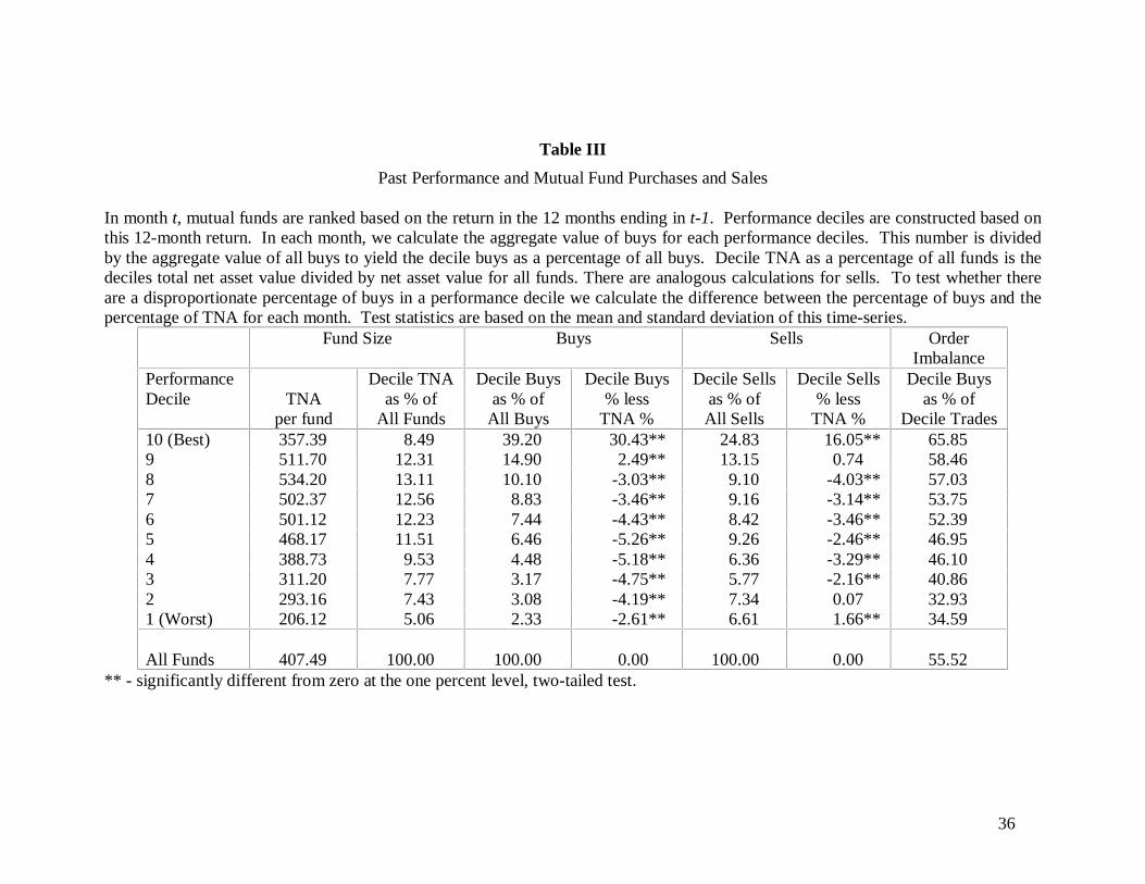
36

Table III

Past Performance and Mutual Fund Purchases and Sales

In month t, mutual funds are ranked based on the return in the 12 months ending in t-1. Performance deciles are constructed based onthis 12-month return. In each month, we calculate the aggregate value of buys for each performance deciles. This number is dividedby the aggregate value of all buys to yield the decile buys as a percentage of all buys. Decile TNA as a percentage of all funds is thedeciles total net asset value divided by net asset value for all funds. There are analogous calculations for sells. To test whether thereare a disproportionate percentage of buys in a performance decile we calculate the difference between the percentage of buys and thepercentage of TNA for each month. Test statistics are based on the mean and standard deviation of this time-series.

Fund Size Buys Sells OrderImbalance

PerformanceDecile TNA

per fund

Decile TNAas % of

All Funds

Decile Buysas % of

All Buys

Decile Buys% less

TNA %

Decile Sellsas % ofAll Sells

Decile Sells% less

TNA %

Decile Buysas % of

Decile Trades10 (Best) 357.39 8.49 39.20 30.43** 24.83 16.05** 65.859 511.70 12.31 14.90 2.49** 13.15 0.74 58.468 534.20 13.11 10.10 -3.03** 9.10 -4.03** 57.037 502.37 12.56 8.83 -3.46** 9.16 -3.14** 53.756 501.12 12.23 7.44 -4.43** 8.42 -3.46** 52.395 468.17 11.51 6.46 -5.26** 9.26 -2.46** 46.954 388.73 9.53 4.48 -5.18** 6.36 -3.29** 46.103 311.20 7.77 3.17 -4.75** 5.77 -2.16** 40.862 293.16 7.43 3.08 -4.19** 7.34 0.07 32.931 (Worst) 206.12 5.06 2.33 -2.61** 6.61 1.66** 34.59

All Funds 407.49 100.00 100.00 0.00 100.00 0.00 55.52** - significantly different from zero at the one percent level, two-tailed test.

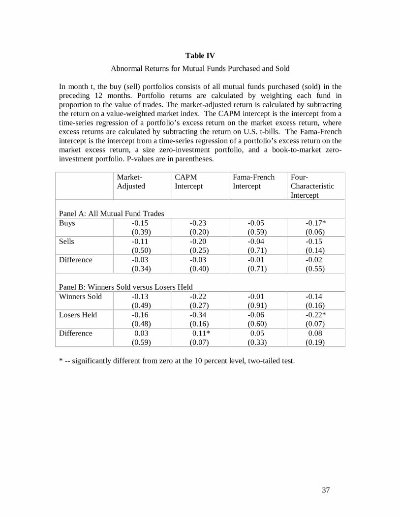
37

Table IV

Abnormal Returns for Mutual Funds Purchased and Sold

In month t, the buy (sell) portfolios consists of all mutual funds purchased (sold) in thepreceding 12 months. Portfolio returns are calculated by weighting each fund inproportion to the value of trades. The market-adjusted return is calculated by subtractingthe return on a value-weighted market index. The CAPM intercept is the intercept from atime-series regression of a portfolio’s excess return on the market excess return, whereexcess returns are calculated by subtracting the return on U.S. t-bills. The Fama-Frenchintercept is the intercept from a time-series regression of a portfolio’s excess return on themarket excess return, a size zero-investment portfolio, and a book-to-market zero-investment portfolio. P-values are in parentheses.

Market-Adjusted

CAPMIntercept

Fama-FrenchIntercept

Four-CharacteristicIntercept

Panel A: All Mutual Fund TradesBuys -0.15

(0.39)-0.23(0.20)

-0.05(0.59)

-0.17*(0.06)

Sells -0.11(0.50)

-0.20(0.25)

-0.04(0.71)

-0.15(0.14)

Difference -0.03(0.34)

-0.03(0.40)

-0.01(0.71)

-0.02(0.55)

Panel B: Winners Sold versus Losers HeldWinners Sold -0.13

(0.49)-0.22(0.27)

-0.01(0.91)

-0.14(0.16)

Losers Held -0.16(0.48)

-0.34(0.16)

-0.06(0.60)

-0.22*(0.07)

Difference 0.03(0.59)

0.11*(0.07)

0.05(0.33)

0.08(0.19)

* -- significantly different from zero at the 10 percent level, two-tailed test.

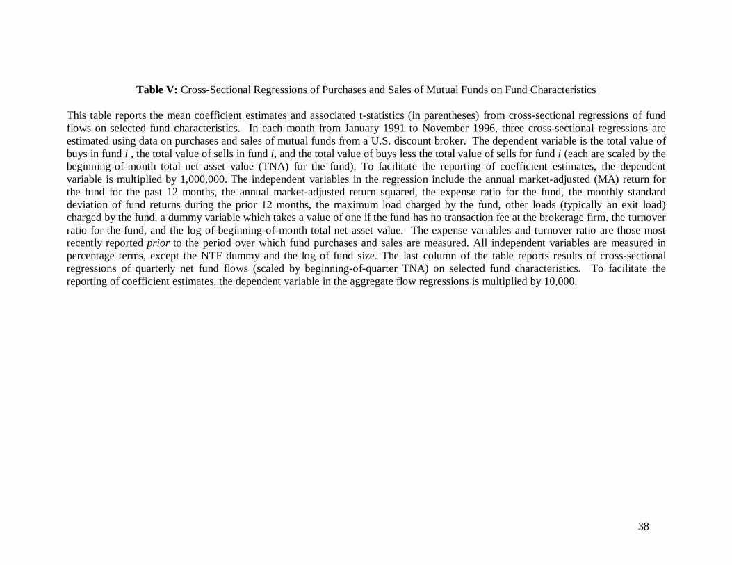
38

Table V: Cross-Sectional Regressions of Purchases and Sales of Mutual Funds on Fund Characteristics

This table reports the mean coefficient estimates and associated t-statistics (in parentheses) from cross-sectional regressions of fundflows on selected fund characteristics. In each month from January 1991 to November 1996, three cross-sectional regressions areestimated using data on purchases and sales of mutual funds from a U.S. discount broker. The dependent variable is the total value ofbuys in fund i , the total value of sells in fund i, and the total value of buys less the total value of sells for fund i (each are scaled by thebeginning-of-month total net asset value (TNA) for the fund). To facilitate the reporting of coefficient estimates, the dependentvariable is multiplied by 1,000,000. The independent variables in the regression include the annual market-adjusted (MA) return forthe fund for the past 12 months, the annual market-adjusted return squared, the expense ratio for the fund, the monthly standarddeviation of fund returns during the prior 12 months, the maximum load charged by the fund, other loads (typically an exit load)charged by the fund, a dummy variable which takes a value of one if the fund has no transaction fee at the brokerage firm, the turnoverratio for the fund, and the log of beginning-of-month total net asset value. The expense variables and turnover ratio are those mostrecently reported prior to the period over which fund purchases and sales are measured. All independent variables are measured inpercentage terms, except the NTF dummy and the log of fund size. The last column of the table reports results of cross-sectionalregressions of quarterly net fund flows (scaled by beginning-of-quarter TNA) on selected fund characteristics. To facilitate thereporting of coefficient estimates, the dependent variable in the aggregate flow regressions is multiplied by 10,000.

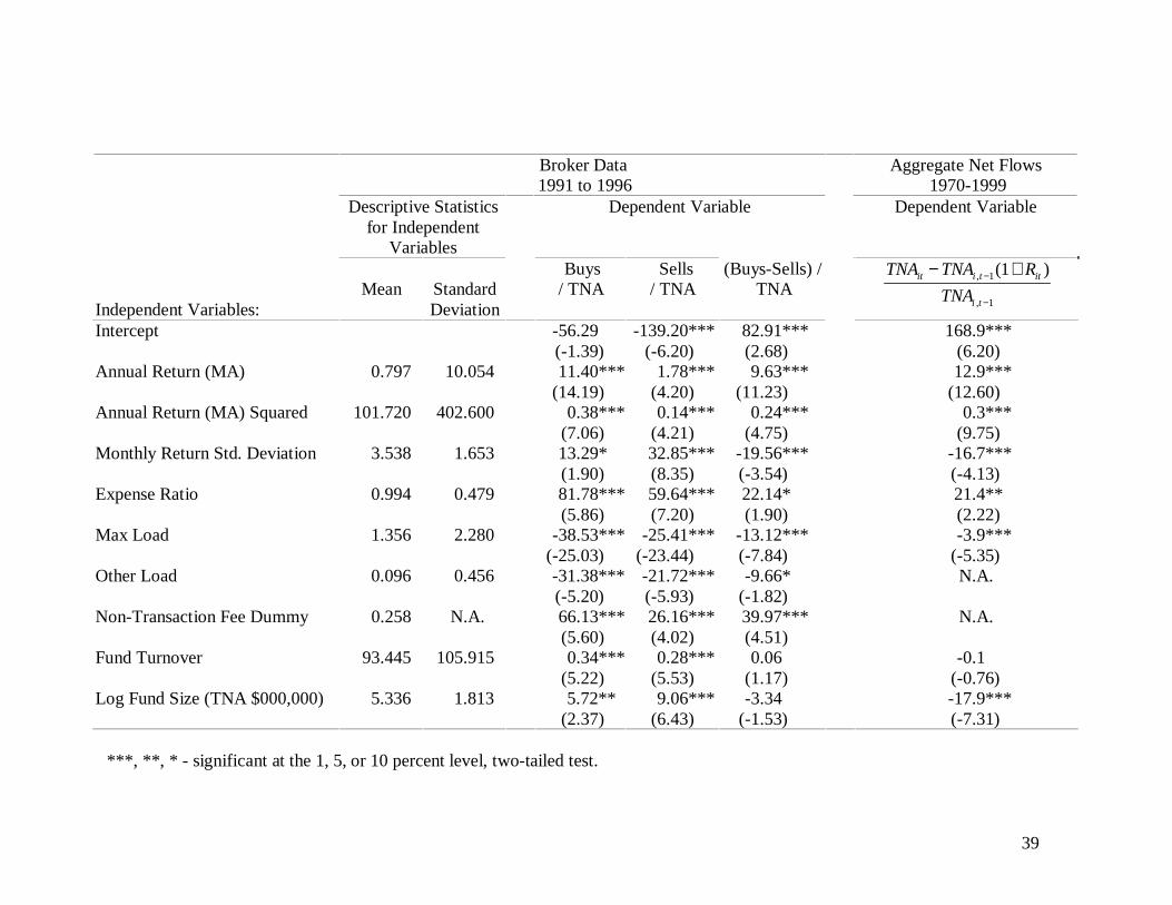
39

Broker Data1991 to 1996

Aggregate Net Flows1970-1999

Descriptive Statisticsfor Independent

Variables

Dependent Variable Dependent Variable

Independent Variables:Mean Standard

Deviation

Buys/ TNA

Sells/ TNA

(Buys-Sells) /TNA

TNA TNA R

TNAit i t it

i t

− +−

−

,

,

( )1

1

1

Intercept -56.29(-1.39)

-139.20***(-6.20)

82.91***(2.68)

168.9***(6.20)

Annual Return (MA) 0.797 10.054 11.40***(14.19)

1.78***(4.20)

9.63***(11.23)

12.9***(12.60)

Annual Return (MA) Squared 101.720 402.600 0.38***(7.06)

0.14***(4.21)

0.24***(4.75)

0.3***(9.75)

Monthly Return Std. Deviation 3.538 1.653 13.29*(1.90)

32.85***(8.35)

-19.56***(-3.54)

-16.7***(-4.13)

Expense Ratio 0.994 0.479 81.78***(5.86)

59.64***(7.20)

22.14*(1.90)

21.4**(2.22)

Max Load 1.356 2.280 -38.53***(-25.03)

-25.41***(-23.44)

-13.12***(-7.84)

-3.9***(-5.35)

Other Load 0.096 0.456 -31.38***(-5.20)

-21.72***(-5.93)

-9.66*(-1.82)

N.A.

Non-Transaction Fee Dummy 0.258 N.A. 66.13***(5.60)

26.16***(4.02)

39.97***(4.51)

N.A.

Fund Turnover 93.445 105.915 0.34***(5.22)

0.28***(5.53)

0.06(1.17)

-0.1(-0.76)

Log Fund Size (TNA $000,000) 5.336 1.813 5.72**(2.37)

9.06***(6.43)

-3.34(-1.53)

-17.9***(-7.31)

***, **, * - significant at the 1, 5, or 10 percent level, two-tailed test.

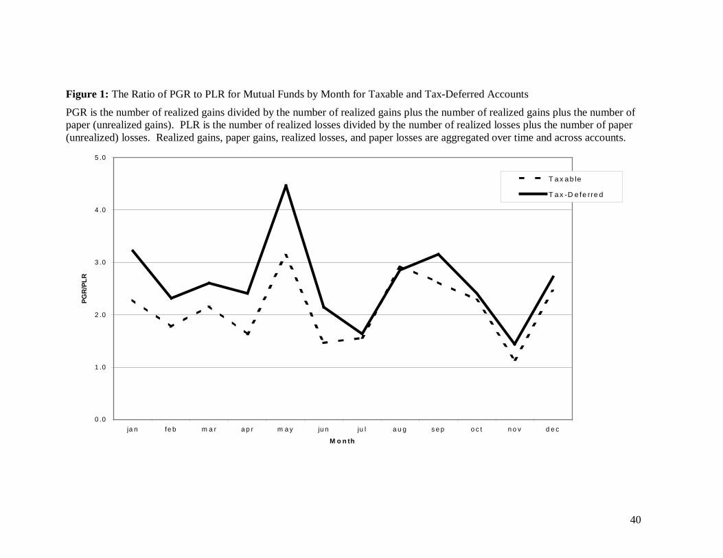
40

Figure 1: The Ratio of PGR to PLR for Mutual Funds by Month for Taxable and Tax-Deferred Accounts

PGR is the number of realized gains divided by the number of realized gains plus the number of realized gains plus the number ofpaper (unrealized gains). PLR is the number of realized losses divided by the number of realized losses plus the number of paper(unrealized) losses. Realized gains, paper gains, realized losses, and paper losses are aggregated over time and across accounts.

0 .0

1 .0

2 .0

3 .0

4 .0

5 .0

ja n fe b m a r a p r m a y ju n ju l a u g s e p o c t n o v d e c

M o n th

PG

R/P

LR

T a x a b le

T a x -D e fe rre d

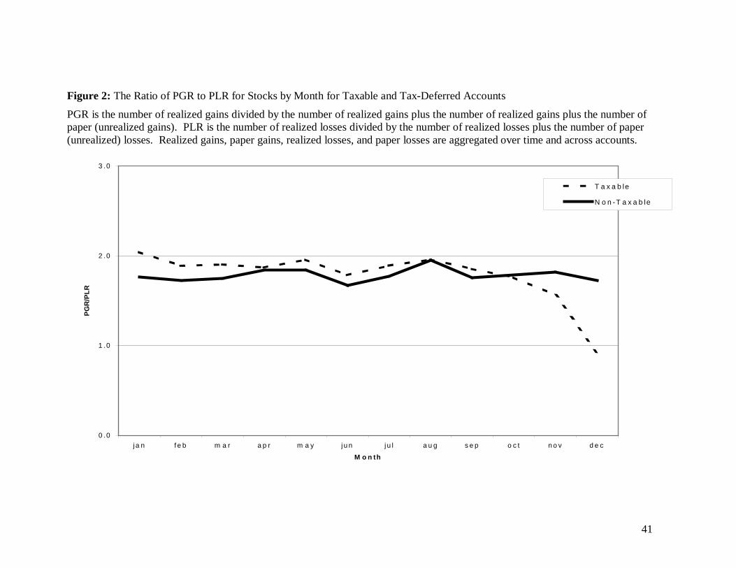
41

Figure 2: The Ratio of PGR to PLR for Stocks by Month for Taxable and Tax-Deferred Accounts

PGR is the number of realized gains divided by the number of realized gains plus the number of realized gains plus the number ofpaper (unrealized gains). PLR is the number of realized losses divided by the number of realized losses plus the number of paper(unrealized) losses. Realized gains, paper gains, realized losses, and paper losses are aggregated over time and across accounts.

0 .0

1 .0

2 .0

3 .0

ja n f e b m a r a p r m a y ju n ju l a u g s e p o c t n o v d e c

M o n th

PG

R/P

LR

T a x a b le

N o n -T a x a b le

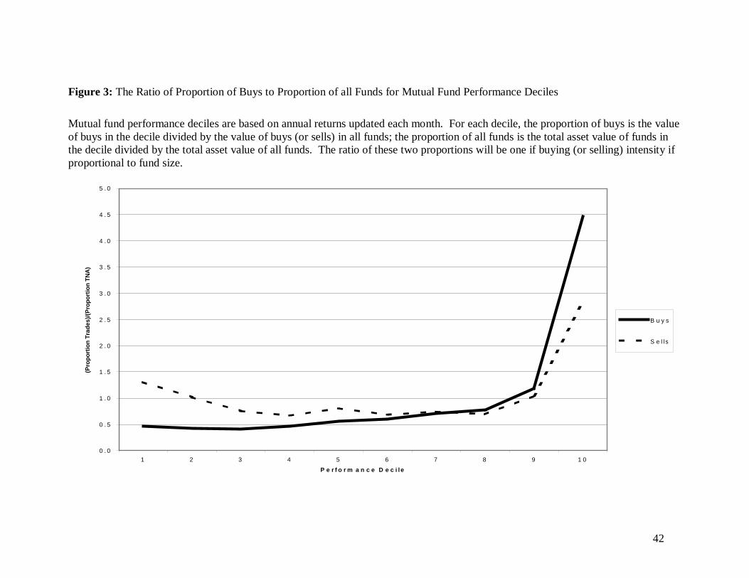
42

Figure 3: The Ratio of Proportion of Buys to Proportion of all Funds for Mutual Fund Performance Deciles

Mutual fund performance deciles are based on annual returns updated each month. For each decile, the proportion of buys is the valueof buys in the decile divided by the value of buys (or sells) in all funds; the proportion of all funds is the total asset value of funds inthe decile divided by the total asset value of all funds. The ratio of these two proportions will be one if buying (or selling) intensity ifproportional to fund size.

0 . 0

0 . 5

1 . 0

1 . 5

2 . 0

2 . 5

3 . 0

3 . 5

4 . 0

4 . 5

5 . 0

1 2 3 4 5 6 7 8 9 1 0

P e r f o r m a n c e D e c i le

(Pro

po

rtio

n T

rad

es)/

(Pro

po

rtio

n T

NA

)

B u y s

S e l ls

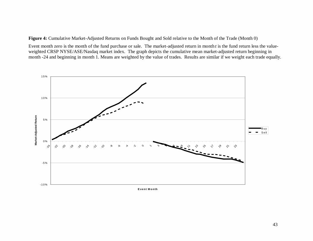
43

Figure 4: Cumulative Market-Adjusted Returns on Funds Bought and Sold relative to the Month of the Trade (Month 0)

Event month zero is the month of the fund purchase or sale. The market-adjusted return in month t is the fund return less the value-weighted CRSP NYSE/ASE/Nasdaq market index. The graph depicts the cumulative mean market-adjusted return beginning inmonth -24 and beginning in month 1. Means are weighted by the value of trades. Results are similar if we weight each trade equally.

-1 0 %

-5 %

0 %

5 %

1 0 %

1 5 %

-24

-22

-20

-18

-16

-14

-12

-10 -8 -6 -4 -2 0 1 3 5 7 9 11 13 15 17 19 21 23

E ve n t M o n th

Mar

ket-

Ad

just

ed R

etu

rn

B uy

S e ll

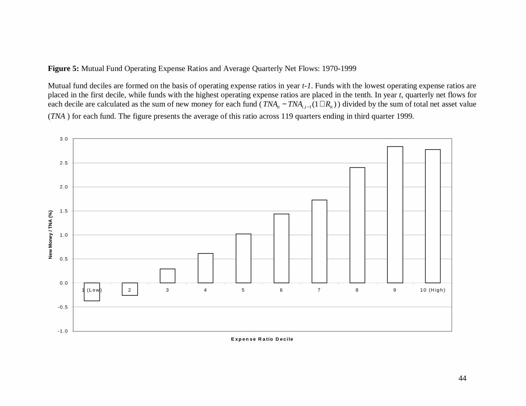
44

Figure 5: Mutual Fund Operating Expense Ratios and Average Quarterly Net Flows: 1970-1999

Mutual fund deciles are formed on the basis of operating expense ratios in year t-1. Funds with the lowest operating expense ratios areplaced in the first decile, while funds with the highest operating expense ratios are placed in the tenth. In year t, quarterly net flows foreach decile are calculated as the sum of new money for each fund ( TNA TNA Rit i t it− +−, ( )1 1 ) divided by the sum of total net asset value

(TNA ) for each fund. The figure presents the average of this ratio across 119 quarters ending in third quarter 1999.

-1 .0

-0 .5

0 .0

0 .5

1 .0

1 .5

2 .0

2 .5

3 .0

1 (L o w ) 2 3 4 5 6 7 8 9 1 0 (H ig h )

E x p e n s e R a tio D e c i le

New

Mo

ney

/ T

NA

(%

)

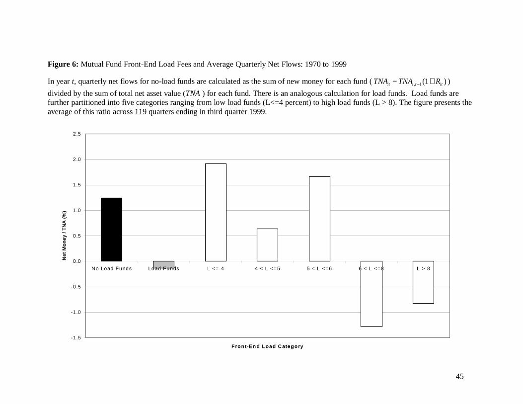
45

Figure 6: Mutual Fund Front-End Load Fees and Average Quarterly Net Flows: 1970 to 1999

In year t, quarterly net flows for no-load funds are calculated as the sum of new money for each fund ( TNA TNA Rit i t it− +−, ( )1 1 )

divided by the sum of total net asset value (TNA ) for each fund. There is an analogous calculation for load funds. Load funds arefurther partitioned into five categories ranging from low load funds (L<=4 percent) to high load funds (L > 8). The figure presents theaverage of this ratio across 119 quarters ending in third quarter 1999.

-1.5

-1.0

-0.5

0.0

0.5

1.0

1.5

2.0

2.5

No Load Funds Load Funds L <= 4 4 < L <=5 5 < L <=6 6 < L <=8 L > 8

Front-En d Load Category

Net

Mo

ney

/ T

NA

(%

)

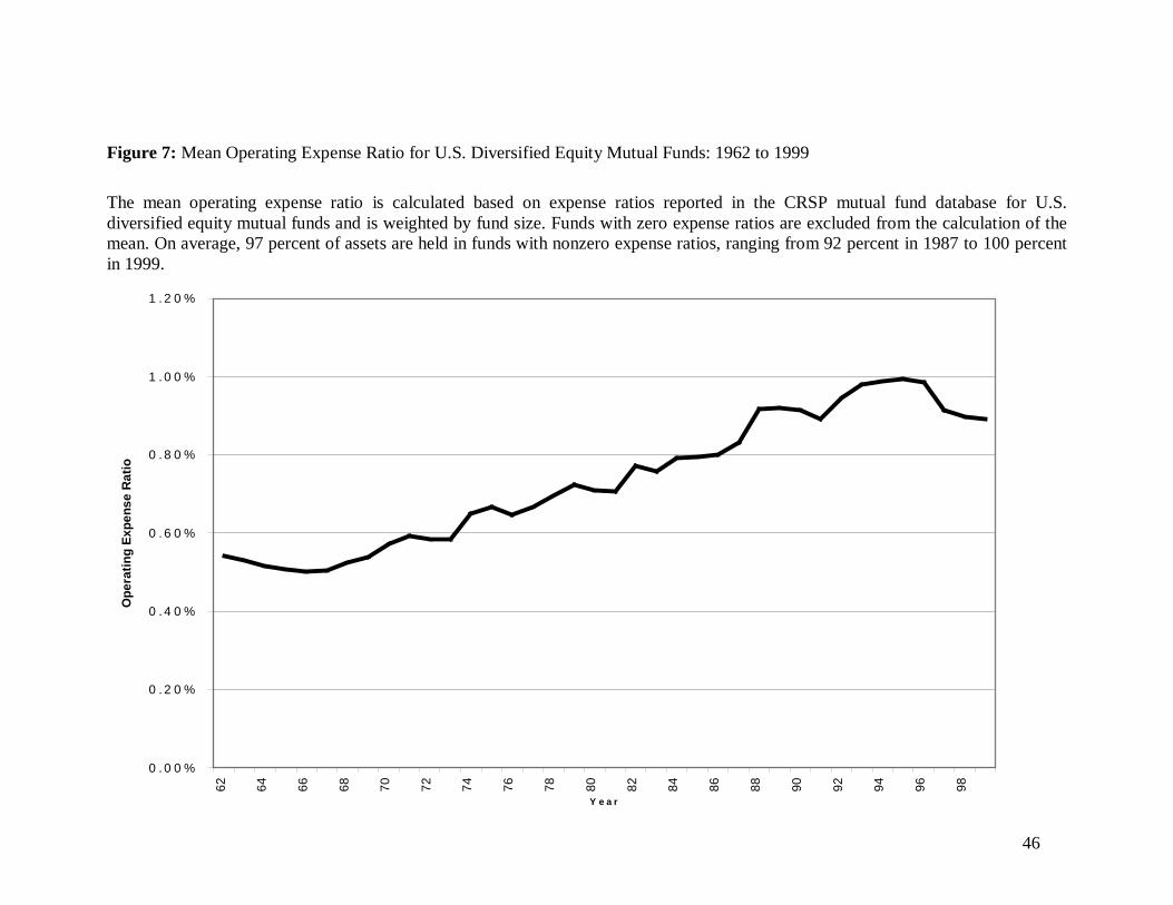
46

Figure 7: Mean Operating Expense Ratio for U.S. Diversified Equity Mutual Funds: 1962 to 1999

The mean operating expense ratio is calculated based on expense ratios reported in the CRSP mutual fund database for U.S.diversified equity mutual funds and is weighted by fund size. Funds with zero expense ratios are excluded from the calculation of themean. On average, 97 percent of assets are held in funds with nonzero expense ratios, ranging from 92 percent in 1987 to 100 percentin 1999.

0 . 0 0 %

0 . 2 0 %

0 . 4 0 %

0 . 6 0 %

0 . 8 0 %

1 . 0 0 %

1 . 2 0 %

62 64 66 68 70 72 74 76 78 80 82 84 86 88 90 92 94 96 98

Y e a r

Op

erat

ing

Exp

ense

Rat

io

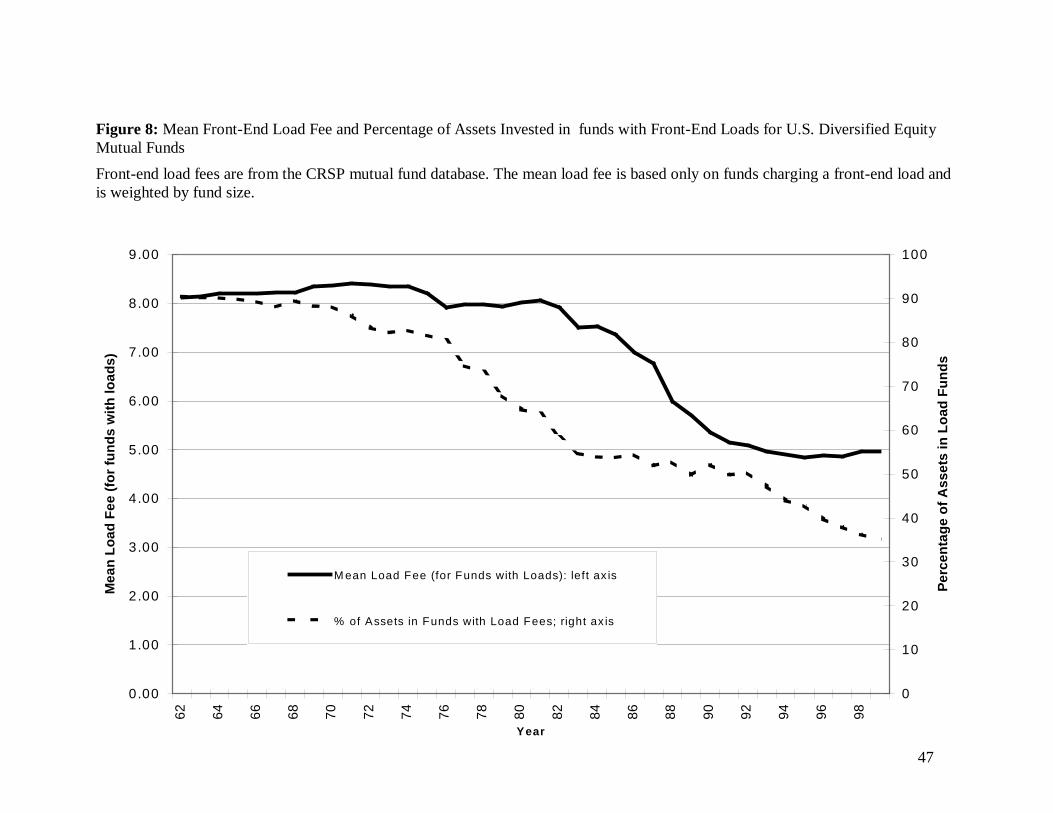
47

Figure 8: Mean Front-End Load Fee and Percentage of Assets Invested in funds with Front-End Loads for U.S. Diversified EquityMutual Funds

Front-end load fees are from the CRSP mutual fund database. The mean load fee is based only on funds charging a front-end load andis weighted by fund size.

0.00

1.00

2.00

3.00

4.00

5.00

6.00

7.00

8.00

9.00

62 64 66 68 70 72 74 76 78 80 82 84 86 88 90 92 94 96 98

Year

Mea

n L

oad

Fee

(fo

r fu

nd

s w

ith

load

s)

0

10

20

30

40

50

60

70

80

90

100

Per

cen

tag

e o

f A

sset

s in

Lo

ad F

un

ds

M ean Load Fee (for Funds with Loads): left ax is

% of Assets in Funds with Load Fees; right ax is