The B.E. Journal of Economic Analysis & Policy · Intergenerational Mobility in Australia∗ Andrew Leigh Abstract Combining four surveys conducted over a forty year period, I calculate

The B.E. Journal of EconomicAnalysis & Policy

Contributions

Volume7, Issue2 2007 Article 6

INTERGENERATIONAL ECONOMIC MOBILITY AROUND THEWORLD

Intergenerational Mobility in Australia

Andrew Leigh∗

∗Australian National University, [email protected]

Recommended CitationAndrew Leigh (2007) “Intergenerational Mobility in Australia,”The B.E. Journal of EconomicAnalysis & Policy: Vol. 7: Iss. 2 (Contributions), Article 6.Available at: http://www.bepress.com/bejeap/vol7/iss2/art6

Copyright c©2007 The Berkeley Electronic Press. All rights reserved.

Intergenerational Mobility in Australia∗

Andrew Leigh

Abstract

Combining four surveys conducted over a forty year period, I calculate intergenerational earn-ings elasticities for Australia, using predicted earnings in parents’ occupations as a proxy for actualparental earnings. In the most recent survey, the elasticity of sons’ wages with respect to fathers’wages is around 0.2. Comparing this estimate with earlier surveys, I find little evidence that inter-generational mobility in Australia has significantly risen or fallen over time. Applying the samemethodology to United States data, I find that Australian society exhibits more intergenerationalmobility than the United States. My method appears to slightly overstate the degree of intergen-erational mobility; if the true intergenerational earnings elasticity in the United States is 0.4–0.6(as recent studies have suggested), then the intergenerational earnings elasticity in Australia isprobably around 0.2–0.3.

KEYWORDS: social mobility, imputed earnings, Australia, United States

∗In part, this paper uses an unconfidentialised unit record file from the Household, Income andLabour Dynamics in Australia (HILDA) survey. The HILDA Project was initiated and is funded bythe Commonwealth Department of Families, Community Services and Indigenous Affairs (FaC-SIA) and is managed by the Melbourne Institute of Applied Economic and Social Research (MI-AESR). The findings and views reported in this paper, however, are those of the author and shouldnot be attributed to either FaCSIA or the MIAESR. Since the data used in this paper are confiden-tial, they cannot be shared with other researchers. However, the Stata do-files are available fromthe author upon request. Elena Varganova provided outstanding research assistance. I am gratefulto Fred Argy, Tue Gørgens, Bob Haveman, Frank Jones, Gary Marks, Bhashkar Mazumder, ChetiNicoletti, Peter Saunders, participants at the ZEW conference on ‘Wage Growth and Mobility’and a La Trobe University seminar, and two anonymous referees for valuable comments on earlierdrafts. Gary Solon provided particularly insightful suggestions, which greatly improved the paper.All remaining errors and omissions are mine.

1. Introduction Australian society has always prided itself in the ease with which individuals can move from one social class to another. Settled as a penal colony, rapid social mobility was the inevitable during the early years. The richest ever Australian (measured relative to GDP) was Samuel Terry, a Manchester thief transported to Australia in 1801. At the time of his death in 1838, Terry had amassed a wealth equivalent to $24 billion in today’s dollars (Rubinstein 2004). The notion of Australia as a country in which one’s life chances were unaffected by one’s parental upbringing was often reflected in comparisons with the United Kingdom. In the mid-1960s, McGregor (1966, 110) argued of Australia that: ‘There is not so much difference between the way the different classes speak, the way they dress or the schools they went to as in England, which makes it easier for individuals to move from social group to group. … … The lack of widespread extremes in social differentiation makes it easy for class-jumpers to “pass”.’1 In this paper, I measure the extent of ‘class jumping’, by estimating the intergenerational earnings elasticity between parents and children. In a perfectly mobile society, there will be no statistically significant relationship between the earnings of parents and children, while in an entirely immobile society, parents and children will occupy precisely the same positions in the earnings distribution. I then compare the degree of intergenerational mobility in Australia in the 2000s with the level in the 1960s, and with intergenerational mobility in the United States. The measure to be estimated is the father-son earnings elasticity. Combining four surveys, conducted in 1965, 1973, 1987 and 2001-04, I analyse the relationship between the earnings of sons born between 1910 and 1979 and the earnings of their fathers. As a proxy for fathers’ earnings, I use predicted occupational earnings. Using the same methodology, I also estimate intergenerational mobility measures for the United States, and use these to benchmark my Australian results. To preview my findings, I find that in the most recent survey, the elasticity of sons’ earnings with respect to their fathers’ earnings is around 0.2. Comparing this with three past surveys, I find no evidence that intergenerational mobility has changed over time in Australia. Applying the same methodology to United States data, I find that Australian society exhibits more intergenerational mobility than

1 In a similar vein, Horne (1964, 61) noted that ‘There are no possibilities in Australia of determining status by simple inspection. You can’t place a man in a social scale by listening to his accent or what he talks about or by looking at his clothes or observing his manners. Ordinary people are not likely to be able to detect a “real gentleman” with that sensory accuracy that used to be characteristic of ordinary people in England.’

1

Leigh: Intergenerational Mobility in Australia

Published by The Berkeley Electronic Press, 2007

the United States, with the largest difference being the mobility of those born into the poorest households. My method appears to slightly overstate the degree of intergenerational mobility. Assuming that the bias from my methodology is the same in the two countries, then if the United States intergenerational earnings elasticity is 0.4–0.6 (as recent studies have suggested), then the true intergenerational earnings elasticity in Australia is likely to be in the range of 0.2-0.3. The remainder of this paper is structured as follows. Section 2 briefly outlines the relevant literature on intergenerational earnings mobility. Section 3 sets out the methodology and data. Section 4 presents results for the four surveys, making it possible to observe how intergenerational mobility has changed over time. Section 5 compares intergenerational mobility in Australia and the United States, and the final section concludes. 2. Existing Studies on Intergenerational Earnings Mobility In the United States, studies in the 1970s and 1980s had tended to estimate father-son earnings elasticities of around 0.2 (Sewell and Hauser 1975; Bielby and Hauser 1977; Behrman and Taubman 1985; Becker and Tomes 1986). However, work by Solon using long-run data from the Panel Study on Income Dynamics (PSID) demonstrated that due to sample bias and errors-in-variables bias, the true elasticity was ‘at least 0.4 and possibly higher’ (Solon 1992, 405). Using social security earnings data over a longer time span, Mazumder (2005) found an elasticity of around 0.6. For daughters, Altonji and Dunn (2000) estimated earnings correlations of 0.27 (mother-daughter) and 0.40 (father-daughter). For family income, Chadwick and Solon (2002) estimated elasticities in the range 0.35 to 0.49. For hourly wages, Altonji and Dunn (2000) estimated correlations in the range 0.35 to 0.41 for the various parent-child combinations. A burgeoning literature has estimated the extent of intergenerational earnings mobility for other countries, including Brazil (Ferriera and Veloso 2006; Dunn 2007), Britain (Atkinson, Maynard and Trinder 1983; Dearden, Machin and Reed 1997; Blanden et al. 2004; Ermisch and Nicoletti 2006), Canada (Fortin and Lefebvre 1998; Corak and Heisz 1999), Finland (Jäntti and Österbacka 1996, Österbacka 2001), Germany (Couch and Dunn 1997, Wiegand 1997; Vogel 2006), Malaysia (Lillard and Kulburn 1995), Nepal (Grawe 2001), Pakistan (Grawe 2001), Peru (Grawe 2001), Sweden (Gustafsson 1994) and South Africa (Hertz 2001). Many of these estimates are based on predicted fathers’ earnings, rather than actual earnings. For Sweden, Björklund and Jäntti (1997) used a two-sample instrumental variables approach to predict earnings using education and

2

The B.E. Journal of Economic Analysis & Policy, Vol. 7 [2007], Iss. 2 (Contributions), Art. 6

http://www.bepress.com/bejeap/vol7/iss2/art6

occupation.2 This approach has been replicated elsewhere, using fathers’ education only (Grawe 2001 for Nepal, Pakistan and Peru; Dunn 2007 for Brazil), fathers’ occupation only (Fortin and Lefebvre 1998 for Canada), and both fathers’ education and fathers’ occupation (Ferriera and Veloso 2006 for Brazil; Ermisch and Nicoletti 2006 for Britain). As Solon (2002) and Corak (2006) have pointed out in their respective reviews of international studies on intergenerational mobility, methodological differences limit comparability between these studies. However, some researchers have sought to benchmark their results against the United States by using as comparable a methodology as possible. Studies by Corak and Heisz (1999), Österbacka (2001) and Gustafsson (1994) have shown that intergenerational earnings mobility in Canada, Finland and Sweden, respectively, is higher than in the United States. A large-scale study by Jäntti et al. (2006) concluded that intergenerational earnings mobility is higher in the United Kingdom than the United States, and higher again in the Nordic countries (Denmark, Finland, Norway and Sweden), with the greatest cross-country differences arising at the tails of the distribution. A small number of studies have also sought to estimate whether intergenerational mobility has risen or fallen since World War II.3 For the United States, three studies have arrived at different conclusions. Mayer and Lopoo (2005) constructed successive cohorts from the PSID and found that social mobility rose for cohorts born during the 1950s and 1960s (though the rise was not statistically significant). Lee and Solon (2006) used the PSID, but constructed overlapping birth cohorts, and found no significant trend in mobility. Aaronson and Mazumder (2008) imputed parental income using parents’ state of birth for cohorts born from 1921-75, and found a fall in intergenerational mobility among cohorts born after the mid-1950s. For the United Kingdom, Blanden et al. (2004) compared two cohorts, comprising all children born during a single week in 1958 with a similar sample for 1970, and concluded that intergenerational mobility in Britain had fallen over time. Ermisch and Nicoletti (2006) used data from the British Household Panel Survey (imputing parental earnings using occupation and education) and also found a fall in mobility, though the change was not statistically significant. In Australia, most of the existing research on intergenerational mobility has appeared in the sociological literature, and has focused on occupational status, rather than imputed earnings. Radford (1962) analysed results from a survey of

2 For further discussion of the Dearden, Machin and Reed (1997) approach, see Abul Naga and Cowell (2002). 3 Ferrie (2005) took a longer view, comparing intergenerational occupational mobility in the United States for sons observed 1880-1900 and sons observed in 1950-1973. He concluded that intergenerational occupational mobility fell substantially over this period.

3



nearly all those who left school in Australia in 1959-60. He found that the fraction of sons entering the same broad occupation as their fathers was 61 percent for farming, 38 percent for skilled trades, 20 percent for semi-skilled or unskilled jobs, and 36 percent for jobs requiring a university education. Surveys of social mobility in Australia that were conducted in 1965 and 1973 formed the basis for further work by Broom et al. (1977, 1980). Other significant studies by sociologists on intergenerational occupational mobility in Australia include Davis (1984), Jones and Davis (1986), Jones, Wilson and Pittelkow (1990), Wanner and Hayes (1996) and Marks and McMillan (2003). I am not aware of any studies to have estimated intergenerational earnings mobility for Australia.4 3. Methodology and Data Following the previous literature, the primary measure of intergenerational mobility used in this paper will be the father-son earnings elasticity. Since suitable long-run panel surveys and samples of social security earnings records are not available for Australia, I instead predict fathers’ earnings using sons’ reports of their fathers’ occupations.5 Such a prediction technique is necessitated by the fact that parental earnings are not directly available in the Australian surveys. It is also desirable, since the use of single-year earnings data has been shown to lead to an overestimate of the level of social mobility in a society. For example, using United States Social Security earnings data for 1951-1991, Haider and Solon (2006) found that the use of single-year earnings led to a considerable underestimate of the true earnings elasticity between fathers and sons. Since fathers’ earnings are not measured directly in the surveys, I predict the earnings of fathers using the occupation in which a respondent’s father was employed when the respondent was aged 14. The number of occupational categories is large, varying from 78 to 241 (see Data Appendix for details). Fathers are then assigned the predicted earnings for a male aged 40 in that occupation. Since fathers’ earnings are proxied using current earnings data, this method means that a 40 year old son who happened to earn precisely the average (age-adjusted) occupational wage would be assigned the same earnings as his father. 4 A recent Australian study to have looked at intergenerational transmission channels is Miller, Mulvey and Martin (2001), who used a sample of Australian twins to estimate the extent to which intergenerational educational correlations are genetically determined. They did not estimate intergenerational earnings elasticities or correlations. 5 The two representative national panel data surveys in Australia are the Negotiating the Life Course Survey, which has been conducted on a triennial basis since 1997, and the Household Income and Labour Dynamics in Australia Survey (HILDA), which has been conducted on an annual basis since 2001.

4



Among employed fathers and sons, three factors drive intergenerational mobility: (i) sons working in different occupations from their fathers (inter-occupational mobility), (ii) sons working in the same occupation but with lower or higher earnings than their fathers (intra-occupational mobility), and (iii) changes in the average earnings of occupations over time. The method employed here will capture inter-occupational mobility (factor i), but will only capture part of intra-occupational mobility (factor ii), since all fathers are assigned the predicted earnings for a 40 year old in their occupation. Moreover, this approach will not take account of changes in the average earnings of occupations over time (factor iii). To the extent that intra-occupational changes or changes in average occupational earnings over time are a major factor in intergenerational mobility, this approach may mis-estimate the true level of intergenerational mobility.6 How does this approach compare with that of Björklund and Jäntti (1997)? While my approach proxies earnings using a large number of occupations, theirs used eight occupational categories, two educational categories, and a regional indicator. Using an earlier survey to obtain a sample of ‘synthetic fathers’, they employed the technique of two-sample instrumental variables to predict the earnings of fathers in the sample.7 In the case of Australia, such an approach is complicated by two factors: changes in occupational coding systems across surveys, and the paucity of earnings survey data prior to the 1970s. (Nonetheless, as a robustness check, I present below the results from an estimation strategy based on matching occupations across two different samples.) Using fine occupational categories to impute earnings may also have advantages over predicting earnings using broad occupational categories plus parental education; or predicting earnings using parental education alone. As Solon (1992) points out, the use of parental education may be problematic if parental education has a direct impact on sons’ earnings, rather than only affecting sons’ earnings through the channel of parental earnings. For example, Solon suggests that one would not want to proxy parental income using parental education if ‘the son of a highly educated clergyman with a moderate income tends to earn somewhat more than the son of a less-educated moderate-income

6 Although I was unable to obtain comparable occupational earnings data for Australia over this period, some sense as to how much this factor might bias the results can be gleaned from looking at changes in the rankings of occupational earnings in the United States. Using microdata from US Censuses to calculate the mean age-adjusted log earnings of men aged 25-54 in 192 occupations, Andrews and Leigh (2008) find that the correlation between an occupation’s mean earnings in 1970 and 2000 was 0.71. While this correlation is reassuringly high, it does suggest that the occupational imputation approach will not perfectly estimate the true extent of intergenerational mobility. 7 For a detailed discussion of two-sample instrumental variables, see Angrist and Krueger (1992).

5



father’ (Solon 1992, 406). By contrast, it is more probable that a father’s occupation affects his son’s earnings primarily through the channel of income.8 If permanent log earnings were observed for both son (ysi) and father (yfi), the intergenerational earnings elasticity δ could simply be estimated by applying OLS to the following equation:

ifisi yy νδγ ++= (1)

However, because earnings are observed at a point in time, it is necessary to control for age. In addition, because information on fathers’ actual earnings is not contained in the survey, it is necessary to predict fathers’ earnings using the average age-adjusted earnings in that occupation. To predict fathers’ earnings, I use data from the current survey, and regress log earnings yij of individual i in occupation j on a vector of occupation dummies Xij, and a quadratic in age Ai:

ijiiijjij AAXy υλλθ +++= 221

' (2)

The log earnings of a father in occupation j are then predicted to be the same as those of a 40 year old in occupation j. Algebraically, where A=40, jjf yy ˆˆ == . The final estimating equation is:

iiijfsi AAyy εϕϕβα ++++= =2

21ˆ (3)

In most specifications, sons’ earnings will be drawn from a single year; but for the most recent survey, I also estimate the impact on intergenerational mobility of predicting fathers’ earnings using data averaged over a four-year period, so as to reduce measurement error in the independent variable. The coefficient β in this equation denotes the intergenerational elasticity, being the percentage change in the son’s earnings for doubling of the father’s earnings. Another common measure of intergenerational mobility is the intergenerational correlation, which is based on estimating the same regression, but with the variance in earnings held constant between the two periods. This 8 In an appendix to their paper, Aaronson and Mazumder (2008) estimate the intergenerational elasticity using NLSY data, first with parental earnings and parental education, and then with parental earnings and parental occupation. They find that parental education remains statistically significant even after including parental earnings (implying a violation of the exclusion restriction), while parental occupation is not statistically significant once parental earnings are included in the regression. This suggests that as an instrument for parental earnings, parental occupation may be preferable to parental education.

6



effectively standardises the elasticity for changes in variance in the two periods, and is thus a measure of an individual’s relative position in the distribution. The relationship between the two measures is a function of the ratio of the standard deviation of log earnings in the two generations:

s

f

σσ

βρ = (4)

Note that when the standard deviation of earnings (net of age) is the same

in both generations (σf = σs), then the intergenerational elasticity will precisely equal the intergenerational correlation. In a period when inequality is changing, both the intergenerational elasticity and the intergenerational correlation may be of interest. For example, if the income distribution is wider in the sons’ generation than the fathers’ generation, then the intergenerational elasticity will be higher than the intergenerational correlation. Empirically, many papers in this literature present only the intergenerational elasticity. Since I do not observe the actual standard deviation of fathers’ earnings, I follow the same approach here, presenting only intergenerational elasticities. However, it is possible to speculate about the relationship between the elasticity and the correlation by drawing on existing studies of long-run trends in inequality in Australia. These studies (e.g. McLean and Richardson 1986; Harding and Greenwell 2002; Leigh 2005; Atkinson and Leigh 2007) show a fall in inequality between the 1940s and the 1970s, and a rise in inequality from the 1970s to the 2000s. In this paper, I use four surveys to estimate earnings mobility, measuring sons’ earnings in 1965, 1973, 1987 and 2004, respectively. Assuming that the trends in aggregate earnings inequality reflect differences in long-run earnings dispersion across cohorts, one would expect that the correlation would be larger than the elasticity for the first two surveys (since σf >σs), and that the correlation would be smaller than the elasticity in the last two surveys (since σf <σs). The four surveys used in this paper permit the calculation of intergenerational mobility for sons born between 1911 and 1979.9 In each of the surveys, sons’ earnings are measured directly (with earnings coded in bands in the 1965 and 1973 surveys, and measured precisely in the 1987 and 2004 surveys). Because of the chosen method of imputing earnings to fathers, I focus on hourly wages rather than annual earnings (though I also show annual earnings as a

9 As is often the case in the intergenerational mobility literature, the estimates are constrained by data availability. In particular, it should be noted that there is considerable overlap between the 1965 and 1973 cohorts, which are perhaps better regarded as a check on one another than as a test of changes in social mobility.

7



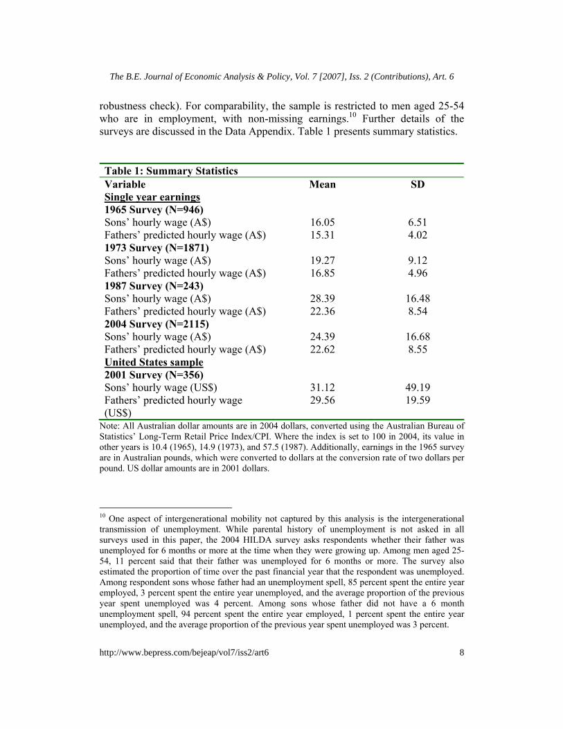
robustness check). For comparability, the sample is restricted to men aged 25-54 who are in employment, with non-missing earnings.10 Further details of the surveys are discussed in the Data Appendix. Table 1 presents summary statistics. Table 1: Summary Statistics Variable Mean SD Single year earnings 1965 Survey (N=946) Sons’ hourly wage (A$) 16.05 6.51 Fathers’ predicted hourly wage (A$) 15.31 4.02 1973 Survey (N=1871) Sons’ hourly wage (A$) 19.27 9.12 Fathers’ predicted hourly wage (A$) 16.85 4.96 1987 Survey (N=243) Sons’ hourly wage (A$) 28.39 16.48 Fathers’ predicted hourly wage (A$) 22.36 8.54 2004 Survey (N=2115) Sons’ hourly wage (A$) 24.39 16.68 Fathers’ predicted hourly wage (A$) 22.62 8.55 United States sample 2001 Survey (N=356) Sons’ hourly wage (US$) 31.12 49.19 Fathers’ predicted hourly wage (US$)

29.56 19.59

Note: All Australian dollar amounts are in 2004 dollars, converted using the Australian Bureau of Statistics’ Long-Term Retail Price Index/CPI. Where the index is set to 100 in 2004, its value in other years is 10.4 (1965), 14.9 (1973), and 57.5 (1987). Additionally, earnings in the 1965 survey are in Australian pounds, which were converted to dollars at the conversion rate of two dollars per pound. US dollar amounts are in 2001 dollars.

10 One aspect of intergenerational mobility not captured by this analysis is the intergenerational transmission of unemployment. While parental history of unemployment is not asked in all surveys used in this paper, the 2004 HILDA survey asks respondents whether their father was unemployed for 6 months or more at the time when they were growing up. Among men aged 25-54, 11 percent said that their father was unemployed for 6 months or more. The survey also estimated the proportion of time over the past financial year that the respondent was unemployed. Among respondent sons whose father had an unemployment spell, 85 percent spent the entire year employed, 3 percent spent the entire year unemployed, and the average proportion of the previous year spent unemployed was 4 percent. Among sons whose father did not have a 6 month unemployment spell, 94 percent spent the entire year employed, 1 percent spent the entire year unemployed, and the average proportion of the previous year spent unemployed was 3 percent.

8



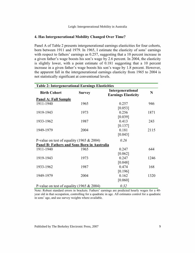
4. Has Intergenerational Mobility Changed Over Time? Panel A of Table 2 presents intergenerational earnings elasticities for four cohorts, born between 1911 and 1979. In 1965, I estimate the elasticity of sons’ earnings with respect to fathers’ earnings as 0.257, suggesting that a 10 percent increase in a given father’s wage boosts his son’s wage by 2.6 percent. In 2004, the elasticity is slightly lower, with a point estimate of 0.181 suggesting that a 10 percent increase in a given father’s wage boosts his son’s wage by 1.8 percent. However, the apparent fall in the intergenerational earnings elasticity from 1965 to 2004 is not statistically significant at conventional levels. Table 2: Intergenerational Earnings Elasticities

Birth Cohort Survey Intergenerational Earnings Elasticity N

Panel A: Full Sample 1911-1940 1965 0.257

[0.053] 946

1919-1943 1973 0.256 [0.039]

1871

1933-1962 1987 0.413 [0.137]

243

1949-1979 2004 0.181 [0.043]

2115

P-value on test of equality (1965 & 2004) 0.26 Panel B: Fathers and Sons Born in Australia 1911-1940 1965 0.247

[0.062] 644

1919-1943 1973 0.247 [0.048]

1246

1933-1962 1987 0.474 [0.196]

168

1949-1979 2004 0.162 [0.060]

1320

P-value on test of equality (1965 & 2004) 0.32 Note: Robust standard errors in brackets. Fathers’ earnings are predicted hourly wages for a 40-year old in that occupation, controlling for a quadratic in age. All estimates control for a quadratic in sons’ age, and use survey weights where available.

9



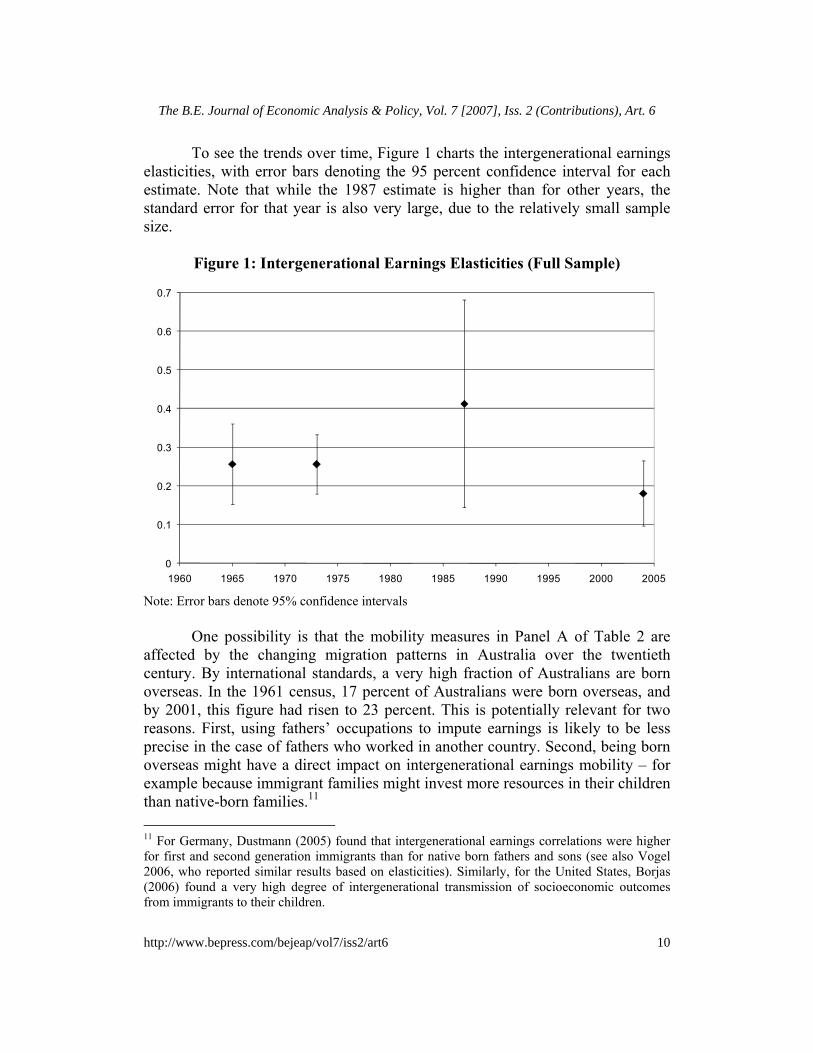
To see the trends over time, Figure 1 charts the intergenerational earnings elasticities, with error bars denoting the 95 percent confidence interval for each estimate. Note that while the 1987 estimate is higher than for other years, the standard error for that year is also very large, due to the relatively small sample size.

Figure 1: Intergenerational Earnings Elasticities (Full Sample)

0

0.1

0.2

0.3

0.4

0.5

0.6

0.7

1960 1965 1970 1975 1980 1985 1990 1995 2000 2005

Note: Error bars denote 95% confidence intervals One possibility is that the mobility measures in Panel A of Table 2 are affected by the changing migration patterns in Australia over the twentieth century. By international standards, a very high fraction of Australians are born overseas. In the 1961 census, 17 percent of Australians were born overseas, and by 2001, this figure had risen to 23 percent. This is potentially relevant for two reasons. First, using fathers’ occupations to impute earnings is likely to be less precise in the case of fathers who worked in another country. Second, being born overseas might have a direct impact on intergenerational earnings mobility – for example because immigrant families might invest more resources in their children than native-born families.11 11 For Germany, Dustmann (2005) found that intergenerational earnings correlations were higher for first and second generation immigrants than for native born fathers and sons (see also Vogel 2006, who reported similar results based on elasticities). Similarly, for the United States, Borjas (2006) found a very high degree of intergenerational transmission of socioeconomic outcomes from immigrants to their children.

10



Panel B of Table 2 therefore excludes from the calculations all respondents who were themselves born overseas, or whose fathers were born overseas. For three of the four surveys (the exception being the 1987 survey) this has the effect of modestly decreasing the intergenerational earnings elasticities, suggesting that natives are perhaps slightly more socially mobile than migrants. Again, the 2004 estimate (0.162) is lower than the 1965 estimate (0.247), but the difference is not statistically significant. In considering whether intergenerational mobility has changed over time, it is important to note two key differences between the different surveys. First, income in some of the surveys is presented in bands, while in others it is a continuous measure. Second, the number of occupations across which fathers are distributed varies from 78 to 241. To take account of these issues, I re-estimate the elasticities after first collapsing income into six bands, and fathers’ occupations into about 80 categories (I leave unchanged the occupational coding of the 1965 survey, with 89 occupations, and the 1987 survey, with 78 occupations). The effect of this is to change the estimates for all years except 1965.

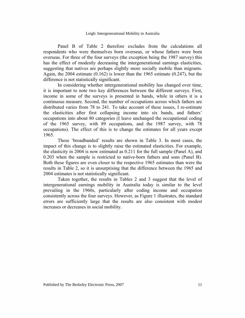
These ‘broadbanded’ results are shown in Table 3. In most cases, the impact of this change is to slightly raise the estimated elasticities. For example, the elasticity in 2004 is now estimated as 0.211 for the full sample (Panel A), and 0.203 when the sample is restricted to native-born fathers and sons (Panel B). Both these figures are even closer to the respective 1965 estimates than were the results in Table 2, so it is unsurprising that the difference between the 1965 and 2004 estimates is not statistically significant. Taken together, the results in Tables 2 and 3 suggest that the level of intergenerational earnings mobility in Australia today is similar to the level prevailing in the 1960s, particularly after coding income and occupation consistently across the four surveys. However, as Figure 1 illustrates, the standard errors are sufficiently large that the results are also consistent with modest increases or decreases in social mobility.

11



Table 3: Robustness Check – Broadbanding Income and Occupation

Birth Cohort Survey Intergenerational Earnings Elasticity N

Panel A: Full Sample 1911-1940 1965 0.257

[0.053] 946

1919-1943 1973 0.280 [0.039]

1871

1933-1962 1987 0.492 [0.090]

243

1949-1979 2004 0.211 [0.041]

2115

P-value on test of equality (1965 & 2004) 0.49 Panel B: Fathers and Sons Born in Australia 1911-1940 1965 0.247

[0.062] 644

1919-1943 1973 0.280 [0.048]

1246

1933-1962 1987 0.583 [0.098]

168

1949-1979 2004 0.203 [0.055]

1320

P-value on test of equality (1965 & 2004) 0.59 Note: Robust standard errors in brackets. Fathers’ earnings are predicted hourly wages for a 40-year old in that occupation, controlling for a quadratic in age. All estimates control for a quadratic in sons’ age, and use survey weights where available. Estimates are based on collapsing the income variable into six categories, and occupations into approximately 80 categories (note that this does not affect the 1965 results).

For the most recent estimate of intergenerational mobility (based on the 2004 survey), I present a number of additional robustness checks. First, I calculate a measure of earnings mobility that is based upon fathers’ earnings in the 1973 survey (a two-sample approach akin to Björklund and Jäntti 1997). The 1973 and 2004 surveys are the best suited for this exercise, since they are the two largest samples utilised here. However, the occupational match is imprecise, owing to significant changes in the coding system, and the fact that some occupational cells are empty in 1973 (necessitating a match to the next most similar occupation). The second robustness check is to restrict the sample to men aged 30-49. The purpose of this is to account for potential ‘lifecycle bias’ in the association between current and permanent income. As Haider and Solon (2006) point out,

12



current earnings are a particularly poor proxy for lifetime earnings for men aged in their twenties (and, to a lesser extent, for men aged in their fifties). Third, since measurement error in fathers’ earnings may lead to a downward bias in the estimated intergenerational earnings elasticity, I exploit the panel structure of the HILDA survey to create occupational predictions for fathers that are based on four-year average hourly wages. Note that this has the effect of slightly reducing the sample size, since there are some occupations in which no respondents had positive hours and earnings in all four years. To maximise sample size, this estimate is still based on single-year earnings for sons (random measurement error in the dependent variable does not bias the slope coefficient). A fourth robustness check is to use annual earnings in place of hourly wages. As noted above, the rationale for using hourly wages in the preferred specification is that earnings are imputed using occupations only. A father’s occupation is likely to be a better predictor of his hourly wage than of his hours (although there may be some systematic variation in hours worked by occupation, much of the variation is likely to be noise).12 Nonetheless, since most estimates of intergenerational mobility in the literature are based on annual earnings, it is useful to also estimate this measure using the present dataset. Table 4 shows the results from these robustness checks, with the main results shown in Panel A for ease of comparison. The two-sample approach (Panel B) has the effect of noticeably increasing the elasticity: to 0.223 for the full sample, and to 0.259 for the native-born sample. Were it not possible to benchmark the Australian estimates against United States estimates (as I do in the next section), then the estimates in Panel B would be the preferred estimates of the current level of intergenerational mobility in Australia. Reassuringly, the benchmarking exercise produces quite similar elasticity estimates to the two-sample approach. Restricting the sample to sons aged 30-49 (Panel C) or using four-year earnings for fathers (Panel D) are approaches that are both aimed at reducing the degree of attenuation bias in the estimates. As might be expected, both have the effect of raising the coefficient on fathers’ earnings, though the estimates are still close to 0.2. Using annual earnings (Panel E) has the effect of slightly lowering the estimated intergenerational elasticity for the full sample (to 0.157). This is most 12 A straightforward way to see this is to decompose annual hours inequality and hourly wage inequality into within-occupation and between-occupation inequality. The more inequality that there is within occupations, the less precisely occupations will proxy wages/earnings. Using the Theil Index, and data from the 2004 HILDA survey (adjusted for age effects), I find that within-occupation inequality accounts for 75% of the variation in annual hours, but 61% of the variation in hourly wages. This higher degree of within-occupational variation in the case of annual hours suggests that an individual’s occupation will be a better proxy for his hourly wage than it will be for his annual earnings (hourly wage × annual hours).

13



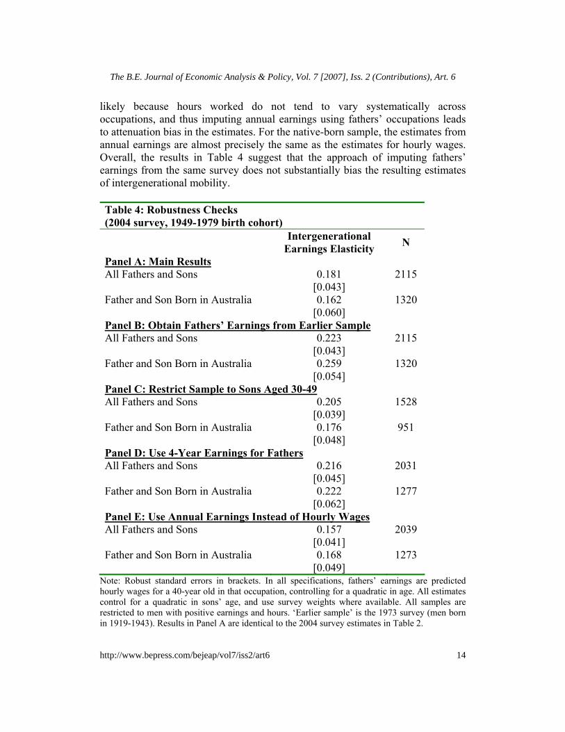
likely because hours worked do not tend to vary systematically across occupations, and thus imputing annual earnings using fathers’ occupations leads to attenuation bias in the estimates. For the native-born sample, the estimates from annual earnings are almost precisely the same as the estimates for hourly wages. Overall, the results in Table 4 suggest that the approach of imputing fathers’ earnings from the same survey does not substantially bias the resulting estimates of intergenerational mobility. Table 4: Robustness Checks (2004 survey, 1949-1979 birth cohort)

Intergenerational Earnings Elasticity N

Panel A: Main Results All Fathers and Sons 0.181

[0.043] 2115

Father and Son Born in Australia 0.162 [0.060]

1320

Panel B: Obtain Fathers’ Earnings from Earlier Sample All Fathers and Sons 0.223

[0.043] 2115


1320

Panel C: Restrict Sample to Sons Aged 30-49 All Fathers and Sons 0.205

[0.039] 1528


951

Panel D: Use 4-Year Earnings for Fathers All Fathers and Sons 0.216

[0.045] 2031


1277

Panel E: Use Annual Earnings Instead of Hourly Wages All Fathers and Sons 0.157

[0.041] 2039


1273

Note: Robust standard errors in brackets. In all specifications, fathers’ earnings are predicted hourly wages for a 40-year old in that occupation, controlling for a quadratic in age. All estimates control for a quadratic in sons’ age, and use survey weights where available. All samples are restricted to men with positive earnings and hours. ‘Earlier sample’ is the 1973 survey (men born in 1919-1943). Results in Panel A are identical to the 2004 survey estimates in Table 2.

14



5. Comparing Intergenerational Mobility in Australia and the United States To benchmark the Australian results, I estimate intergenerational earnings elasticities for the United States using the same methodology, thus facilitating a direct comparison between the two countries. The 2001 wave of the Panel Study of Income Dynamics (PSID) asked respondents for the occupation of their father when they were growing up. Restricting the sample to men aged 25-54 with positive earnings results in a sample of 356 respondents, whose fathers are spread across 86 occupations. Of these, 41 percent of the sons are first-generation or second-generation immigrants. This is partly due to the fact that the PSID includes a Latino sample and an immigrant sample, both of which were added during the 1990s (survey weights ensure that these groups do not receive disproportionate emphasis in the estimates). The native-born specification comprises 211 pairs in which both the father and son are born in the United States. Table 5 shows the intergenerational elasticities; first for the full sample, and then for the native-born. For the full sample, the intergenerational earnings elasticity is 0.325 for the United States and 0.181 for Australia. The difference between the two elasticities is statistically significant, though only at the 10 percent level. However, when the sample is restricted to native-born fathers and sons, the intergenerational earnings elasticity falls substantially for the United States, making the two coefficients statistically indistinguishable. In both countries, migrants appear to be less socially mobile than natives, but the difference is much more pronounced for the United States than for Australia. Focusing only on pairs where the father and son are native-born, social mobility appears to be similar in the two nations.

15



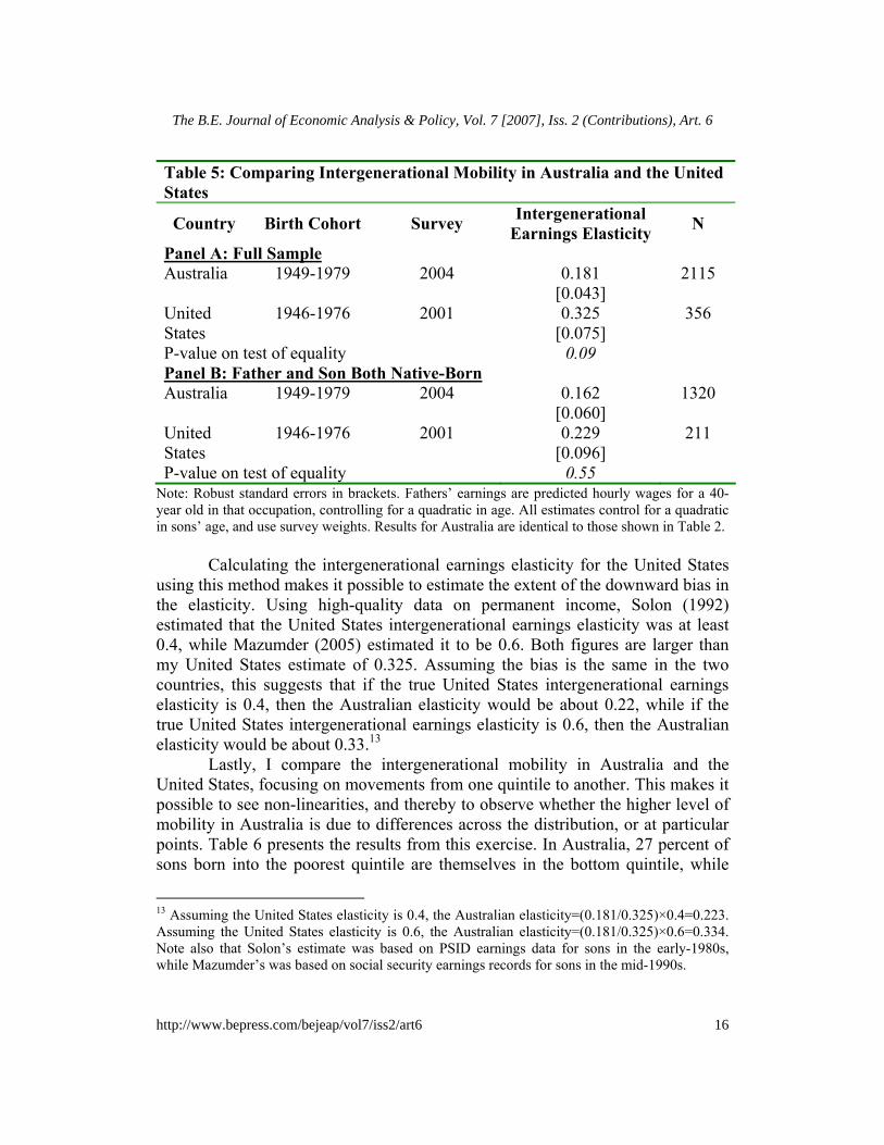
Table 5: Comparing Intergenerational Mobility in Australia and the United States

Country Birth Cohort Survey Intergenerational Earnings Elasticity N

Panel A: Full Sample Australia 1949-1979 2004 0.181

[0.043] 2115

United States

1946-1976 2001 0.325 [0.075]

356

P-value on test of equality 0.09 Panel B: Father and Son Both Native-Born Australia 1949-1979 2004 0.162

[0.060] 1320

United States

1946-1976 2001 0.229 [0.096]

211

P-value on test of equality 0.55 Note: Robust standard errors in brackets. Fathers’ earnings are predicted hourly wages for a 40-year old in that occupation, controlling for a quadratic in age. All estimates control for a quadratic in sons’ age, and use survey weights. Results for Australia are identical to those shown in Table 2.

Calculating the intergenerational earnings elasticity for the United States using this method makes it possible to estimate the extent of the downward bias in the elasticity. Using high-quality data on permanent income, Solon (1992) estimated that the United States intergenerational earnings elasticity was at least 0.4, while Mazumder (2005) estimated it to be 0.6. Both figures are larger than my United States estimate of 0.325. Assuming the bias is the same in the two countries, this suggests that if the true United States intergenerational earnings elasticity is 0.4, then the Australian elasticity would be about 0.22, while if the true United States intergenerational earnings elasticity is 0.6, then the Australian elasticity would be about 0.33.13 Lastly, I compare the intergenerational mobility in Australia and the United States, focusing on movements from one quintile to another. This makes it possible to see non-linearities, and thereby to observe whether the higher level of mobility in Australia is due to differences across the distribution, or at particular points. Table 6 presents the results from this exercise. In Australia, 27 percent of sons born into the poorest quintile are themselves in the bottom quintile, while

13 Assuming the United States elasticity is 0.4, the Australian elasticity=(0.181/0.325)×0.4=0.223. Assuming the United States elasticity is 0.6, the Australian elasticity=(0.181/0.325)×0.6=0.334. Note also that Solon’s estimate was based on PSID earnings data for sons in the early-1980s, while Mazumder’s was based on social security earnings records for sons in the mid-1990s.

16



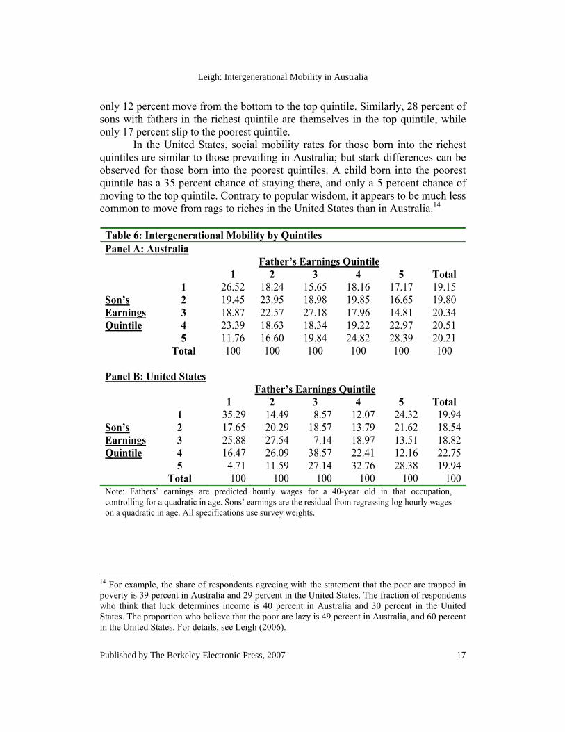
only 12 percent move from the bottom to the top quintile. Similarly, 28 percent of sons with fathers in the richest quintile are themselves in the top quintile, while only 17 percent slip to the poorest quintile. In the United States, social mobility rates for those born into the richest quintiles are similar to those prevailing in Australia; but stark differences can be observed for those born into the poorest quintiles. A child born into the poorest quintile has a 35 percent chance of staying there, and only a 5 percent chance of moving to the top quintile. Contrary to popular wisdom, it appears to be much less common to move from rags to riches in the United States than in Australia.14

Table 6: Intergenerational Mobility by Quintiles Panel A: Australia Father’s Earnings Quintile 1 2 3 4 5 Total 1 26.52 18.24 15.65 18.16 17.17 19.15 Son’s 2 19.45 23.95 18.98 19.85 16.65 19.80 Earnings 3 18.87 22.57 27.18 17.96 14.81 20.34 Quintile 4 23.39 18.63 18.34 19.22 22.97 20.51 5 11.76 16.60 19.84 24.82 28.39 20.21 Total 100 100 100 100 100 100 Panel B: United States Father’s Earnings Quintile 1 2 3 4 5 Total 1 35.29 14.49 8.57 12.07 24.32 19.94Son’s 2 17.65 20.29 18.57 13.79 21.62 18.54Earnings 3 25.88 27.54 7.14 18.97 13.51 18.82Quintile 4 16.47 26.09 38.57 22.41 12.16 22.75 5 4.71 11.59 27.14 32.76 28.38 19.94 Total 100 100 100 100 100 100Note: Fathers’ earnings are predicted hourly wages for a 40-year old in that occupation, controlling for a quadratic in age. Sons’ earnings are the residual from regressing log hourly wages on a quadratic in age. All specifications use survey weights.

14 For example, the share of respondents agreeing with the statement that the poor are trapped in poverty is 39 percent in Australia and 29 percent in the United States. The fraction of respondents who think that luck determines income is 40 percent in Australia and 30 percent in the United States. The proportion who believe that the poor are lazy is 49 percent in Australia, and 60 percent in the United States. For details, see Leigh (2006).

17



6. Conclusion Combining four surveys over a forty year period, I estimate the extent of intergenerational earnings mobility in Australia. In the most recent survey, I estimate that for fathers and sons, the intergenerational elasticity is about 0.2. However, applying the same method to United States data suggests that this empirical strategy may overestimate the extent of intergenerational mobility in Australia. If the true United States intergenerational earnings elasticity is 0.4, and the bias is the same in the two countries, then the Australian figure is likely to be around 0.22. If the true United States intergenerational earnings elasticity is 0.6, then the Australian figure is likely to be around 0.33. This suggests that if an Australian father’s earnings increased by 10 percent, his son’s earnings would rise by 2-3 percent. Combining this result with that of Jäntti et al. (2006) suggests that Australia is probably less socially mobile than the Scandinavian countries, and possibly about as socially mobile as the United Kingdom. There is little evidence that intergenerational mobility has changed over time in Australia (although the confidence intervals are sufficiently large that I am unable to rule out modest trends in either direction). On one view, the absence of any significant rise in intergenerational mobility might be regarded as surprising. Increases in health care coverage, the banning of racial discrimination, the abolition of up-front university tuition fees, and an increase in the number of university places are among the policy reforms that might have been expected to increase intergenerational mobility. Yet there were also trends in the opposite direction. Rising unemployment, the abolition of federal inheritance taxes in 1979, and rising spatial concentration of joblessness (Gregory and Hunter 1995) are among the factors that might have acted to reduce intergenerational mobility. Moreover, the well-documented rise in inequality in Australia (Harding and Greenwell 2002; Leigh 2005) means that the distance between income quintiles was larger in the early-2000s than in the mid-1960s. Data Appendix In all cases, the sample was restricted to men aged 25-54 with positive earnings and hours. Where income was provided in bands, amounts were coded to the midpoint of the band, and the top income amount was recoded to 1.15 times the upper limit. Where provided, sample weights were used. 1965 Social stratification in Australia The sampling frame for this survey was men aged 21 or over in the paid workforce, living in one of 23 randomly selected federal electorates. The survey

18



was conducted by personal interview, and is not restricted to those on the electoral roll (which is used only to identify a starting address). No information about the response rate is provided in the codebook. Sample weights are not provided. The sample is mostly men, but it does comprise a small number of women (who are excluded from the analysis). Fathers are spread across 89 occupations. Income is annual income, measured in six bands. Income is coded to the midpoint of the band, and 115% of the upper limit for the top band. Hours are only supplied as full-time, which I assume to be 1920 hours per year, and part-time, which I assume to be 960 hours per year. For more information about this survey, see Broom, Jones, and Zubrzycki (1965). 1973 Social mobility in Australia project The sampling frame for this survey was men and women aged 30-69 years in private dwellings. The sampling was carried out using a three-stage stratification technique, with a booster sample of areas thought likely to contain more recent immigrants (see codebook for details). The survey was conducted by personal interview, with a response rate of around 70 percent. Survey weights are provided (specifically, I use the population weight variable). The microdata for this survey are separated into two files by gender, and I use the male file. The sample is restricted to men aged 30 and over. Fathers are spread across 214 occupations. Income is the respondent’s weekly income, in 16 bands. Income is coded to the midpoint of the band, and 115% of the upper limit for the top band. Hourly wages are calculated as earnings divided by hours. For more information about this survey, see Broom et al. (1973). 1987-1988 National Social Science Survey The sampling frame for this survey was adults on the Australian electoral roll (since voter registration is compulsory in Australia, the number of registered voters closely tracks the number of adult citizens). The survey was a mail-out survey, with a response rate of 60 percent. Sample weights are not provided. Fathers are spread across 78 occupations. Income is reported in dollars, and the sample is restricted to those for whom income was reported on an annual basis, and who were working full-time or part-time. Hours are only supplied as full-time, which I assume to be 1920 hours per year, and part-time, which I assume to be 960 hours per year. For more information about this survey, see Kelley, Bean, and Evans (1988). 2001-04 Household, Income and Labour Dynamics in Australia (HILDA) survey The initial sampling frame for this survey was private dwellings in Australia. Households were selected via a three-stage approach, which involved selecting

19



Census Collection Districts, then dwellings, then households. Respondents in the first wave are followed even if they establish new households. The data were mostly collected via face-to-face interviews, supplemented in some cases with telephone interviews. In the first wave, 65 percent of the households in the sample were successfully contacted. In waves 2, 3 and 4, the household response rates were 87, 82, and 79 percent, respectively. Cross-sectional and longitudinal weights are provided (specifically, I use dhhwtrp for estimates based upon 2004 data, and dlnwte for estimates based on 2001-04 data). Fathers are spread across 241 occupations. Earnings are current weekly gross wages and salary in main job. Hours are hours per week in the main job. Hourly wages are calculated as earnings divided by hours. For more detail about the HILDA survey, see Watson (2006). Other Australian surveys, including the various Australian Election Studies, the 1984-88 National Social Science Survey, the 1986 Social Mobility survey, and the 1987 Australian Standard of Living Study, were considered and rejected for this paper. Details as to why each of these studies were considered inferior to those used here are available from the author on request. United States Panel Study of Income Dynamics (PSID) The initial sampling frame for the PSID in 1968 consisted of two samples: a nationally-representative sample drawn from the Survey Research Center (SRC), and a low-income oversample from the Survey of Economic Opportunity (SEO). Due to concerns about the representativeness of the SEO sample, I follow Lee and Solon (2006), and drop it from my analysis. In 1990 and 1992, a Latino sample was added to the PSID, and in 1997 and 1999, an immigrant sample was added. I include these additional samples in my analysis. For the initial sample and additional samples, the PSID follows members of the original family units and their adult offspring, even if they leave their original households. All observations are weighted using population weights. For simplicity, I use the Cross-National Equivalent File version of the PSID (for background on the CNEF, see Burkhauser et al. 2001), and merge in the variable for father’s occupation. Fathers are spread across 111 occupations. Full-time employment is coded as working more than 1750 hours per year (coded as e1110101 by the CNEF). Income is annual individual labor earnings for 2001 (coded as i1111001 by the CNEF), divided by hours worked. Occupations are 3-digit codes, using the 1970 occupational coding system. They are drawn from the 2001 wave of the PSID (codes er17226 for sons, and er19959 for fathers).

20



References Aaronson, D. and Mazumder, B. 2008. ‘Intergenerational Economic Mobility in the U.S., 1940 to 2000’ Journal of Human Resources, forthcoming. Abul Naga, R. and Cowell, F.A. 2002. ‘Intergenerational Mobility in Britain: Revisiting the Prediction Approach of Dearden, Machin and Reed’ Discussion Paper DARP 62. London: London School of Economics and Political Science, Distributional Analysis Research Programme. Altonji, J.G. and Dunn, T.A. 2000. ‘An Intergenerational Model of Wages, Hours, and Earnings’ Journal of Human Resources 35(2): 221-258. Andrews, D. and Leigh, A. 2008. ‘More Inequality, Less Social Mobility’ Applied Economics Letters, forthcoming. Angrist, J. and Krueger, A. 1992. ‘The Effect of Age at School Entry on Educational Attainment: An Application of Instrumental Variables with Moments from Two Samples’ Journal of the American Statistical Association 87(418): 328-336. Atkinson, A.B. and Leigh, A. 2007. ‘The Distribution of Top Incomes in Australia’ Economic Record 83(262): 247-261. Atkinson, A.B., Maynard, A.K. and Trinder, C.G. 1983. Parents and Children: Incomes in Two Generations. London: Heinemann. Becker, G.S and Tomes, N. 1986. ‘Human Capital and the Rise and Fall of Families’ Journal of Labor Economics 4(3): S1-S39. Behrman, J.R. and Taubman, P. 1985. ‘Intergenerational Earnings Mobility in the United States: Some Estimates and a Test of Becker’s Intergenerational Endowment Model’ Review of Economics and Statistics 67(1): 144-151. Bielby, W.T. and Hauser, R.M. 1977. ‘Response Error in Earnings Functions for Nonblack Males’ Sociological Methods and Research 6: 241-280. Björklund, A. and Jäntti, M. 1997. ‘Intergenerational Income Mobility in Sweden Compared to the United States’ American Economic Review 87(5) 1009-1018.

21



Blanden, J. Goodman, A., Gregg, P. and Machin, S. 2004. ‘Changes in Intergenerational Mobility in Britain’ In M. Corak (ed.) Generational Income Mobility in North America and Europe. Cambridge: Cambridge University Press, 122-146. Borjas, G.J. 2006. ‘Making it in America: Social Mobility in the Immigrant Population’ The Future of Children 16(2): 55-71. Broom, L., Jones, F.L. and Zubrzycki, J. 1965. Social Stratification in Australia, 1965 [computer file]. ASSDA Study 7. Canberra: Australian Social Science Data Archive, Australian National University. Broom, L., Duncan-Jones, P., Jones, F.L, McDonnell, P. and Williams, T. 1973. Social Mobility in Australia Project, 1973 [computer file]. ASSDA Study 8. Canberra: Australian Social Science Data Archive, Australian National University. Broom, L., Duncan-Jones, P., Jones, F.L. and McDonnell, P. 1977. ‘Investigating Social Mobility’ Department Monograph 1. Canberra: Department of Sociology, Research School of Social Sciences, Australian National University. Broom, L., Jones, F.L., McDonnell, P. & Williams, T. 1980. The Inheritance of Inequality. London: Routledge and Kegan Paul. Burkhauser, R.V., Butrica, B.A., Daly, M.C. and Lillard, D.R. 2001. ‘The Cross-National Equivalent File: A product of cross-national research’ In I. Becker, N. Ott, and G. Rolf (eds.) Soziale Sicherung in einer dynamischen Gesellschaft: Festschrift fuer Richard Hauser zum 65. Geburtstag Papers in Honor of the 65th Birthday of Richard Hauser. Chadwick, L. and Solon, G. 2002. ‘Intergenerational Income Mobility among Daughters’ American Economic Review 92(1): 335-344. Corak, M. 2006. ‘Do Poor Children Become Poor Adults? Lessons from a Cross Country Comparison of Generational Earnings Mobility’ Research on Economic Inequality 13(1): 143-188. Corak, M. and Heisz, A. 1999. ‘The Intergenerational Earnings and Income Mobility of Canadian Men: Evidence from Longitudinal Income Tax Data’ Journal of Human Resources 34(3): 504-533.

22



Couch, K.A. and Dunn, T.A. 1997. ‘Intergenerational Correlations in Labor Market Status: A Comparison of the United States and Germany’ Journal of Human Resources 32(1): 210-232. Davis, P. 1984. ‘Social Mobility and Class Structure in Australia and New Zealand’. Paper presented to the Australian and New Zealand Association for the Advancement of Science. Dearden, L., Machin, S. and Reed, H. 1997. ‘Intergenerational Mobility in Britain’ Economic Journal 107(440): 47-66. Dunn, C.E. 2007. ‘The Intergenerational Transmission of Lifetime Earnings: Evidence from Brazil’ The B.E. Journal of Economic Analysis & Policy 7(2): Article 2. Available at: http://www.bepress.com/bejeap/vol7/iss2/art2. Dustmann, C. 2005. ‘Intergenerational Mobility and Return Migration: Comparing the sons of foreign and native born fathers’. CReAM Discussion Paper No 05/05. London: Centre for Research and Analysis of Migration, Department of Economics, University College London. Ermisch J. and C. Nicoletti. 2006. ‘Intergenerational earnings mobility: Changes across cohorts in Britain’. mimeo. Institute for Social and Economic Research, University of Essex. Ferreira, S. and Veloso, F. 2006. ‘Intergenerational Mobility of Wages in Brazil’ Brazilian Review of Econometrics 26(2): 181-211. Ferrie, J.P. 2005. ‘The End of American Exceptionalism? Mobility in the United States Since 1850’ Journal of Economic Perspectives 19(3): 199-215. Fortin, N.M. and Lefebvre, S. 1998. ‘Intergenerational Income Mobility In Canada’ In M. Corak (ed.) Labour Markets, Social Institutions, and the Future of Canada’s Children, Statistics Canada, Ottawa, 51-64. Grawe, N., 2001. ‘Intergenerational Mobility in the US and Abroad: Quantile and Mean Regression Measures’. Ph.D. Dissertation, Department of Economics, University of Chicago. Gregory, R.G. and Hunter, B. 1995. ‘The Macro-Economy and the Growth of Ghettos and Urban Poverty in Australia’ Centre for Economic Policy Research Discussion Paper 325, Canberra: Australian National University.

23



Gustafsson, Bjorn. 1994. ‘The Degree and Pattern of Income Immobility in Sweden’ Review of Income and Wealth. 40(1): 67–86. Haider, S.J. and Solon, G. 2006. ‘Life-Cycle Variation in the Association between Current and Lifetime Earnings’ American Economic Review, 96(4): 1308-1320. Harding, A and Greenwell, H. 2002. ‘Trends in Income and Expenditure Inequality in the 1980s and 1990s – A Re-Examination and Further Results’ Discussion Paper 57. Canberra: NATSEM. Hertz, T.N. 2001. Education, Inequality and Economic Mobility in South Africa. Ph.D. Thesis, Amherst, MA: University of Massachusetts. Horne, D. 1964. The Lucky Country: Australia in the Sixties. Ringwood, VIC: Penguin. Jäntti, M. and Österbacka, E. 1996. ‘How Much of the Variance in Income Can Be Attributed to Family Background? Evidence from Finland’ Unpublished. Jäntti, M., B. Bratsberg, K. Røed, O. Raaum, R. Naylor E. Österbacka, A. Björklund, T. Eriksson. 2006. ‘American Exceptionalism in a New Light: A Comparison of Intergenerational Earnings Mobility in the Nordic Countries, the United Kingdom and the United States’ IZA Discussion Paper 1938. Bonn: Institute for the Study of Labor. Jones, F.L. and Davis, P. 1986. Models of Society: Class, Stratification and Gender in Australia and New Zealand. Sydney: Croom Helm. Jones, F.L., Wilson, S.R. and Pittelkow, Y. 1990. ‘Modelling mobility: the use of simulation to choose between near-equivalent models’ Quality and Quantity 24(2): 189-212. Kelley, J., Bean, C., and Evans, M. 1988. National Social Science Survey 1987-1988: Inequality ASSDA Study No. 627. Canberra: Australian National University, Social Science Data Archives. Lee, C. and Solon, G. 2006. ‘Trends in Intergenerational Income Mobility’ NBER Working Paper 12007. Cambridge, MA: National Bureau of Economic Research.

24



Leigh, A, 2005, ‘Deriving Long-Run Inequality Series from Tax Data’ Economic Record 81(255): S58-S70. Leigh, A. 2006. ‘Diversity, Trust and Redistribution’ Dialogue 25(3):43-49. Lillard, L.A. and Kilburn, M.R. 1995. ‘Intergenerational Earnings Links: Sons and Daughters’ RAND Labor and Population Program Paper 95-17. Santa Monica, CA: RAND. McGregor, C. 1966. Profile of Australia. London: Hodder and Stoughton. McLean, I. and Richardson, S. 1986. ‘More or Less Equal? Australian Income Distribution in 1933 and 1980’ Economic Record 62(1): 67-81. Marks, G. and McMillan, R. 2003. ‘Declining inequality? The changing impact of socio-economic background and ability on education in Australia’ British Journal of Sociology 54(4): 453-471. Mayer, S. and Lopoo, L. 2005. ‘Has the Intergenerational Transmission of Economic Status Changed?’ Journal of Human Resources 40(1): 169-185. Miller, P., Mulvey, C. and Martin, N. 2001. ‘Genetic and environmental contributions to educational attainment in Australia’ Economics of Education Review 20(3): 211-224. Österbacka, E. 2001. ‘Family Background and Economic Status in Finland’ Scandinavian Journal of Economics 103(3): 467-484. Osterberg, T. 2000. ‘Intergenerational Income Mobility in Sweden: What Do Tax-Data Show?’ Review of Income and Wealth 46(4): 421-436. Radford, W.C. 1962. School Leavers in Australia 1959-60. Melbourne: Australian Council for Educational Research. Rubinstein, W.D. 2004. The All-Time Australian 200 Rich List. Sydney: Allen and Unwin. Sewell, W.H. and Hauser, R.M. 1975. Education, Occupation and Earnings: Achievements in the Early Career. New York: Academic Press.

25



Solon, Gary. 1992. ‘Intergenerational Income Mobility in the United States’ American Economic Review 82(3): 393-408. Solon, G. 2002. ‘Cross-Country Differences in Intergenerational Earnings Mobility’ Journal of Economic Perspectives 16(3): 59-66. Vogel, T. 2006. ‘Reassessing intergenerational mobility in Germany: some new estimation methods and a comparison of natives and immigrants’, mimeo, Berlin: Department of Economics, Humboldt-Universität zu Berlin. Watson, N. (ed). 2006. HILDA User Manual – Release 4.0, Melbourne: Melbourne Institute of Applied Economic and Social Research, University of Melbourne. Wanner, R.A. and Hayes, B.C. 1996. ‘Intergenerational Occupational Mobility Among Men in Canada and Australia’ Canadian Journal of Sociology 21(1): 43-76. Wiegand, J. 1997. ‘Intergenerational Earnings Mobility in Germany.’ mimeo.

26



Documents

The B.E. Journal of Economic Analysis & Policy · Intergenerational Mobility in Australia∗ Andrew Leigh Abstract Combining four surveys conducted over a forty year period, I calculate