Embed Size (px)
Citation preview

The Bank of England Quarterly Model
Richard Harrison, Kalin Nikolov, Meghan Quinn, Gareth Ramsay,Alasdair Scott and Ryland Thomas

Further copies of this publication are available, at £10 plus p&p, from:
Publications GroupTelephone: 020 7601 4030email: [email protected]
The Bank of England’s website is at www.bankofengland.co.uk
A pdf file of this book and an ASCII file containing the model equations are available at:www.bankofengland.co.uk/publications/beqm/
Bank of England, Threadneedle Street, London, EC2R 8AH
c Bank of England 2005
ISBN 1 85730 153 6

Contents
Foreword 1
Acknowlegements 3
1 Introduction and overview 5
1.1 The role of models and forecasts at the Bank of England 5
1.2 An overview of BEQM 6
1.3 Some key technical features of BEQM 8
1.4 The structure of this book 9
1.5 Summary 10
2 Project motivation and model design 11
2.1 Motivations and challenges 11
2.2 The design of BEQM 12
2.3 A comparison with other models 15
2.4 Summary 18
3 The core theory 23
3.1 Overview 23
3.2 Characterisation of the agents 26
3.3 Characterisation of the markets 38
3.4 The nominal side of the economy and monetary transmission 44
3.5 Long-run growth 49
3.6 Summary 50
4 The core/non-core hybrid approach 61
4.1 Functional forms 62
4.2 Making the hybrid system work 63
4.3 Summary 67
5 Implementing and solving the model 69
5.1 Setting up the model 69
5.2 Solving the model 74
5.3 Recursive simulations 75
5.4 Applications 79
5.5 Summary 83
i

6 Parameterisation and evaluation 85
6.1 Issues in parameterising the core model 85
6.2 The model-consistent database 86
6.3 Parameterising the structural core model 97
6.4 Parameterising the non-core equations 113
6.5 An evaluation of the model’s forecast performance 121
6.6 Summary 126
7 Model properties 127
7.1 Interpreting the responses 127
7.2 Shock responses 128
7.3 Summary 150
8 Final remarks 151
References 153
Appendices
A The core model 165
A.1 Mnemonics 165
A.2 Core model equations 172
B The non-core equations 197
B.1 Mnemonics 197
B.2 Non-core equations 203
C Data transformations and sources 225
D Parameter and exogenous values 243
ii
List of figures
2.1 The trade-off between theory and data 12
2.2 A stylised forecast sequence 15
3.1 Key agents in the model macroeconomy 24
3.2 Key flows and assets 25
3.3 Consumption equilibrium in the steady state 27
3.4 Consumption and net foreign asset equilibrium 29
3.5 Production-clearing flows and stocks 39
3.6 The monetary transmission mechanism 49
5.1 Timing conventions for bonds 69
5.2 Timing convention for housing 70
5.3 Timing convention for capital stock 71
5.4 Building a profile under recursive simulations 76
6.1 Ratios of expenditures to private sector output 106
6.2 Ratios of stock values to private sector output 107
6.3 Relative prices 107
6.4 Comparison of growth rate forecasts from BEQM and the MTMM 123
6.5 Theil inequality coefficients 124
6.6 Comparison of growth rate forecasts from the BEQM core and the MTMM 125
7.1 Effects of an interest rate shock 130
7.2 How expectations can affect shock responses 132
7.3 Effects of a productivity shock 135
7.4 Effects of a government spending shock 139
7.5 Effects of a terms of trade shock 142
7.6 Effects of a world demand shock 145
7.7 Effects of a participation shock 148
iii

List of tables
6.1 The mapping from data to model concepts 90
6.2 The mapping from labour market data to model concepts 97
6.3 Statistical tests for stationarity of gaps 115
A.1 Endogenous variables 165
A.2 Exogenous variables 168
A.3 Parameters 169
A.4 Working variables 171
B.1 Endogenous variables 197
B.2 Exogenous variables 201
B.3 Parameters 202
C.1 Data sources and transformations for BEQM 225
D.1 Parameter values 243
v


List of technical boxes
1 Some recent developments towards hybrid structural models 19
2 The consumer’s maximisation problem 30
3 Private sector output and government output 36
4 Over-discounting and insurance against mortality 42
5 The determination of inflation 46
6 How does the Blanchard-Yaari model make consumption stationary? 51
7 The firm’s maximisation problem 54
8 The union bargaining problem 58
9 The hybrid approach applied to the Ramsey model 64
10 The exogenous variables model 78
11 Conditioning nominal interest rate paths 80
12 Detrending and model units 88
13 The sensitivity of the steady state to changes in parameter values 103
vii


Foreword
This book contains details of the Bank of England’s new quarterly model which is used to help theMonetary Policy Committee produce its economic projections. The book builds on the previous bookson the Bank’s use of economic models.
The new quarterly model is a valuable addition to the Bank’s ‘suite of models’. It does not represent asignificant shift in the Committee’s view of how the economy functions or of the transmissionmechanism of monetary policy. Rather its value lies in the fact that its more consistent and clearlyarticulated economic structure better captures the MPC’s vision of how the economy functions and soprovides the Committee with a more useful and flexible tool to aid its deliberations. The project todevelop a new quarterly model has been an important initiative and I am grateful to all the Bank staffwho contributed to its success. The Bank has an outstanding group of economists and they are theunsung heroes and heroines of the success of the United Kingdom’s new monetary framework.
But all economic models, however good, represent simplifications of reality and, as such, no singlemodel can possibly address the many and varied issues that matter for economic policy. Thisrecognition is central to the Bank’s use of economic models and its approach to economic forecasting.The Bank relies on a plurality of models to help inform the Committee’s projections. And these modelsare used as tools to help the Committee reach the economic judgements that play a critical role inshaping its projections, rather than simply to generate mechanical forecasts. Economic forecasting isultimately a matter of judgement.
The economy is constantly changing and so too will the quarterly model and the other models used bythe Bank. The model described in this book is part of an evolving process and the Bank will continue todevote resources to both reaping the benefits from the advances this new model brings and developing itfurther.
Mervyn King, Governor of the Bank of EnglandJanuary 2005
1


Acknowledgements
The authors would like to thank Mark Allan, Pedro Alvarez-Lois, Charles Bean, Andy Blake, FabioCanova, Spencer Dale, Rebecca Driver, Karen Dury, Philip Evans, Guillermo Felices, GeorgeKapetanios, Hashmat Khan, Lavan Mahadeva, Stephen Millard, Andrew Moniz, Adrian Pagan, LauraPiscitelli, Simon Price, James Proudman, Peter Sinclair, Jan Vlieghe, Peter Westaway, SimonWren-Lewis and Tony Yates for comments on drafts of this material, and Andrew Holder for his work aseditor.
We would also like to thank our successors as forecasters and model users – in particular, James Bell,Alex Brazier, Michael Grady, and Iain de Weymarn – for their work during the transition to the newmodel.
The views expressed in this book are those of the authors and should not be thought to represent those ofthe Monetary Policy Committee.
3


Chapter 1 Introduction and overview
The Bank of England has developed a new macroeconomic model for use in preparing the MonetaryPolicy Committee’s quarterly economic projections. The new Bank of England Quarterly Model(BEQM) was used to an increasing extent during 2003 and is the main tool in the suite of modelsemployed by the staff and the Monetary Policy Committee (MPC) in the construction of the projectionscontained in the quarterly Inflation Report.
This book explains the motivation for BEQM and the economic and modelling approaches underlying it;it also includes a full technical account of the model and its quantitative properties. This chapter (1)
describes the role of models at the Bank of England in helping to produce the MPC’s quarterlyprojections, explains the motivation for the new model, and provides an overview of BEQM and themodelling approaches underlying it. It also includes a guide to the remaining chapters, which describeBEQM in greater detail.
1.1 The role of models and forecasts at the Bank of England
The Bank of England is mandated by the Chancellor of the Exchequer to aim at an inflation target – atthe time of writing, a 2% annual inflation rate of the Consumer Prices Index (CPI) – and uses a veryshort-term nominal interest rate as its instrument to pursue this target. Because of the lags betweenchanges to interest rates and the associated effects on inflation, setting monetary policy is inherently aforward-looking exercise. Hence the quarterly Inflation Report, in addition to assessing the current stateof the economy, contains projections for output growth and inflation for up to three years out, based onassumptions of both constant and market-based interest rates. These projections represent theCommittee’s best judgement of both the most likely central outcome and the range of possiblealternative outcomes around that central case. A key element of the analysis contained in the InflationReport is to consider the major risks and uncertainties surrounding the central projection, rather than tofocus simply on the central point predictions for GDP growth and inflation.
The Bank uses numerous economic models to help produce these projections. (2) No model can doeverything – all models are imperfect, precisely because they are simplifications of reality. And eachprojection is a judgement of the MPC rather than a mechanical output from any model. Nonetheless theBank has found, like many other policy institutions, that, when producing its economic projections, it ishelpful to use a macroeconomic model as the primary organisational framework to process the variousjudgements and assumptions made by the Committee. This is the role now played by BEQM.
The forecast process at the Bank involves a high degree of interaction between the Bank’s staff and themembers of the Monetary Policy Committee. In particular, a key element of the forecast process is forCommittee members to assess the extent to which different economic judgements and assumptionsconcerning the major issues affecting the economy could influence their view of future prospects. Thisprocess is critical to understanding the nature of the risks and uncertainties surrounding the centralprojection. In order to be able to carry out this sort of analysis, the main forecast model ideally needs arelatively explicit economic structure that identifies the key behavioural parameters and channels withinthe economy.
(1) This chapter is based on the article on the new model that was published in the Summer 2004 Quarterly Bulletin, see Bankof England (2004).(2) The Bank’s use of economic models is discussed in more detail in Chapter 1 of Bank of England (1999a).
5

The Bank of England Quarterly Model
The importance of having a model suitable for analysing the implications of different economicjudgements and assumptions is not new. This role was also central to the design of the previous macromodel used by the Bank, the Medium-Term Macro Model (MTMM). (3) Indeed, the basic economicstructure of BEQM is very similar to that of the MTMM. The aim of BEQM is not to incorporate adifferent view of how the economy works or of the role of monetary policy. Rather, the decision todevelop a new model reflected the view that recent advances in both economic understanding and,importantly, in computational power meant that it was possible to improve upon the articulation of theeconomic structure within the MTMM. As Pagan (2003) noted in his report on modelling andforecasting at the Bank of England, the MTMM was no longer ‘state of the art’. In particular, Paganconcluded that ‘It seems highly likely that [a new model] could achieve the same empirical coherence[as the MTMM] with a stronger theoretical perspective’. In doing so, this would provide the Committeewith a more flexible and coherent framework to aid its economic deliberations. That, in short, is whatthe new model tries to achieve through a clearer articulation of the underlying structure of the economyand a more explicit identification of the role expectations play.
1.2 An overview of BEQM
BEQM describes the behaviour of the UK economy at a relatively aggregated level that is closely relatedto the incomes and expenditures recorded in the UK National Accounts. To do this, the model containsformal descriptions of the behaviour of private domestic agents, policymakers and the rest of the world,and their interactions in markets for capital and financial assets, goods, and labour.
Households consume imported and domestically produced goods. When deciding on their current levelof consumption, and hence their level of saving or borrowing, households are assumed to want to keeptheir lifetime consumption as smooth as possible. To do this, households can borrow and save using arange of financial assets, including domestic equities, corporate debt, government debt, money, andforeign assets. In addition, in the short run, households’ levels of consumption can be influenced by avariety of other factors, such as short-term fluctuations in their income and their level of confidenceabout the future.
Firms seek to maximise profits by hiring labour and buying capital in order to produce output. Firms andworkers bargain over wages and, given the outcome, firms are assumed to choose the labour they wish toemploy so that the costs of any extra workers are compensated for by the higher revenues they generate.Similarly, firms’ desired level of capital is determined by the cost of capital and the return to extrainvestment. The output that firms produce is sold in markets for domestic consumption, investment andgovernment procurement, as well as in housing and export markets. Firms are assumed to face varyingdegrees of competition in these markets, which implies that firms may receive a different profit marginfrom the sale of their goods in each market. The composition of total sales will therefore affect revenueand profits, so that relative demand conditions will matter as well as overall demand conditions. Firmsface competition from importers for consumption and investment goods, and have to price their productsin export markets so as to achieve maximum profits. In addition, various short-run factors can influencefirms’ behaviour, such as the short-run prospects for demand affecting the speed with which they invest.
The government buys output from domestic firms and labour from households, financed by raising taxesand selling debt, in addition to a small amount of revenue that accrues from seigniorage. Total revenuealso has to be sufficient to pay the cost of servicing the existing level of government debt and anygovernment transfers. For long-run solvency, the fiscal authority may at some stage have to adjust apolicy instrument – such as a tax rate – to ensure that the fiscal budget constraint is met. A variety of
(3) The Medium-Term Macro Model is described in more detail in Bank of England (2000).
6

Introduction and overview
fiscal policy ‘rules’ can be considered. In general, these rules assume that any required fiscal adjustmentoccurs only gradually.
The monetary policy maker has the job of anchoring the nominal side of the economy. The nominaltarget could, in principle, be specified in terms of any nominal aggregate, such as the nominal exchangerate, the growth rate of nominal output, or the growth rate of the money stock. The default assumptionis that the central bank targets an annual inflation rate of the CPI of 2%, using the short nominal interestrate as its instrument. An assumption about the policy rule used by the central bank – the monetarypolicy reaction function – is required for inflation to be anchored in the long run. The structure allows avariety of different reaction functions to be incorporated.
BEQM assumes that UK capital markets are ‘small’, in the sense that the demand for and supply offinancial assets in the United Kingdom do not affect the level of interest rates prevailing in the rest of theworld. Since all claims on domestic firms’ assets and government debt must ultimately be held either bydomestic households or the rest of the world, it follows that the United Kingdom’s net foreign assetposition is determined jointly by the decisions of firms and the government about how many financialliabilities to issue and by domestic households about how many of these assets to hold. The rest of theworld affects these decisions through assumptions about the level of foreign real interest rates and worlddemand.
These decisions also have implications for the United Kingdom’s trade balance. Suppose, for example,UK households were assumed to want to hold only some of the domestic financial assets on offer, suchthat the United Kingdom maintained a net debt with the rest of the world. This would imply that, in thelong run, the United Kingdom would need to have a trade surplus sufficient to meet the costs ofservicing this debt. The equilibrium real exchange rate moves so as to ensure that exports and importsachieve this long-run balance. This story is further complicated by the assumption that UK producershave some market power in the prices they set in world markets, so the long-run trade balance will, ingeneral, depend on assumptions made about conditions in both financial and goods markets.
The main channels through which changes in monetary policy are transmitted to the rest of the economyare similar to those previously described by the Monetary Policy Committee. (4) The fact that prices andnominal wages move only slowly means that the central bank, by changing the nominal interest rate, hasthe ability to influence real interest rates. Lower real rates tend to encourage consumers to spend morenow. Lower real rates also encourage investment and spending on housing by lowering financing costs,and they make it less costly to hold inventories. The combined effect is to push up domestic demand. Tomeet that demand, firms will demand more of the factors used in the production of goods and services,namely capital and labour. This in turn is likely to increase the costs of these factors of production.
The fact that the UK economy is a small open economy adds an important channel through whichmonetary policy operates. In particular, a lower domestic real interest rate may tend to encourage adepreciation in the real exchange rate. This will lead to both a direct price effect – the prices of importedgoods will rise – and a number of possible indirect (or ‘second-round’) effects, reflecting both anypass-through from higher import prices onto domestic prices and costs, and the impact of any change incompetitiveness associated with the change in the real exchange rate on the United Kingdom’s tradebalance.
The impact of changes in aggregate demand on prices and inflation will depend on the way in whichagents – households, firms, policymakers and the rest of the world – interact with each other. Other
(4) See Bank of England (1999b).
7

The Bank of England Quarterly Model
things being equal, increased demand for workers leads to higher wage costs, which firms will typicallyattempt to pass on to some degree in the form of higher prices. Similarly, increases in world prices or anexchange rate depreciation create pressure on import prices. And increased demand for domesticallyproduced goods will also create incentives for firms to raise prices.
Inflationary pressures reflect the degree of imbalance between the level of demand and the capacity offirms to meet that demand. The level of demand and potential supply will depend on both the currentstance of monetary policy and the stance expected in the future. Likewise, firms’ responses to thesepressures on capacity will depend on the extent to which they are likely to persist, and hence on theexpected stance of monetary policy in the future. The importance of future expectations in determiningcurrent inflationary pressures underlines the central importance of monetary policy anchoring privatesector expectations of the long-term inflation rate.
1.3 Some key technical features of BEQM
The improved economic structure of BEQM is reflected in a number of specific features. First, it has awell defined steady state. This means that, in the long run, all variables in the model settle on paths thatare growing consistently with each other in a sustainable equilibrium. This aids analysis of economicissues, since an understanding of the medium term requires an understanding not just of short-run forces,but also of where the economy is heading to in the long run. For example, a stable steady-state solutionwould not be compatible with a situation in which household debt was increasing without bound.
In characterising this steady state, careful attention has been paid to ‘stock-flow’ and ‘flow-flow’accounting. This is designed to ensure that all economic flows within the economy are accounted for –all income is spent or saved, for example – and that all expenditures have implications for physical andfinancial stocks. This again aids the understanding of medium-term issues. For example, stock-flowconsistency implies that monetary policy cannot stimulate consumption indefinitely, since this wouldimply an erosion of households’ net wealth, which they could not ignore forever.
Another important feature of the new model is that it contains more explicit forward-lookingrepresentations of agents’ expectations about the future. These include expectations about future labourincome, aggregate demand, the exchange rate, and so on. Models with fully forward-looking agents cansometimes exhibit unrealistic dynamic properties; in particular, if households and firms are assumed tohave perfect foresight, they might adjust their behaviour immediately in response to future anticipatedevents. But in reality the economy does not ‘jump’ about in this fashion. That partly reflects the factthat it is often costly for households and firms to change their behaviour very rapidly. In addition, firmsand households do not have perfect foresight. Instead, they have to form expectations on the basis oflimited information. BEQM incorporates both of these features. In particular, it is structured in such away that assumptions about the speed of adjustment and the amount of information available to agentscan be changed in order to help the Committee to assess how these assumptions could affect the futurepath of the economy.
These features are not new: some or all of them are present in many other models currently used bypolicy institutions, such as the Bank of Canada’s Quarterly Projection Model, the FRB/US model at theUS Federal Reserve Board of Governors, and the Reserve Bank of New Zealand’s FPS model. Indeed,these features were often an explicit aim of pioneering work on macro modelling in the United Kingdomover the past 25 years, such as the Liverpool model, the London Business School model, the COMPACTmodel, and various models at the Cambridge Economic Policy Group and the National Institute ofEconomic and Social Research. The implementation in BEQM may differ in technical details, reflecting
8

Introduction and overview
decisions made on how to satisfy the particular demands of forecasting at the Bank, but the basic ideasand motivations are the same.
1.4 The structure of this book
This book explains the factors which led the Bank to develop a new model and the way it went aboutdoing this. In doing so, it provides a thorough technical description of the new model, including detailsof its theory, construction and use. The main text of the chapters is written with the intention of avoidingheavily technical expositions. In some parts, where there are issues that may need more detailedexplanation, use is made of boxes, which can be read or passed by as the reader chooses. Technicaldetails are contained in appendices. The following provides a guide to the remaining chapters.
Chapter 2 contains a fuller discussion of the particular requirements made upon forecasting models atthe Bank of England and how that is reflected in the design of BEQM. The aim of the project was thatthe new model should provide a richer, more explicit, theoretical structure, while matching the data atleast as well as the previous macro model. It would also need to be flexible and reliable under differentforecasting assumptions and conventions. This led us to the concept of building the model with twoparts – a layer that provides the theoretical core of the model, and a layer of extra dynamics designed, inpart, to facilitate judgemental adjustments. The idea of adding ad hoc or ‘data-driven’ dynamics totheoretical structure is not a new one, but the implementation has many variations. The chaptertherefore includes comparisons with alternative modelling approaches and some other macro models.
Chapter 3 discusses the core theory. The individual building blocks of the theoretical core are largelyconventional, as seen in Section 1.2. However, a key focus in the development of BEQM was ensuringthat the model works consistently as a system, with close attention paid to the constraints and linkagesbetween agents.
Chapter 4 follows with an account of the ad hoc dynamics. These equations take the paths from the coretheory and combine them, if needed, with extra persistence and variables that proxy for effects missingin the core theory. These effects might be missing because we choose not to attempt to model them in afully structural way: the additional structure to do so consistently would make the model much morecomplicated and potentially difficult to run. Additionally, there are some effects that seem empiricallyrobust, but are very difficult to model formally.
Chapter 5 provides technical details of how we solve the model. A key issue here is the treatment ofexpectations, and in particular how to deal with cases in which agents do not fully anticipate futureevents. We address this issue by the use of so-called ‘recursive simulations’ that potentially limit theamount of information available to agents from period to period.
Chapter 6 discusses the parameterisation of the model. The main problem that we face is that the modelis large, in order to be able to handle typical forecast issues with sufficient richness. And in order totreat the theoretical building blocks in the model consistently, the model is highly simultaneous – inother words, one agent’s actions will generally depend on all other agents’ actions at the same time. Themodel is therefore too large to confront using conventional econometric techniques for estimatingsimultaneous systems. This issue is not new and confronts all builders of large macro models. Ourapproach is to separate out parameterisation from evaluation. That is, we select parameter values basedon a range of evidence, and then evaluate the whole system against a number of different criteria. Themodel is parameterised to achieve a plausible long-run relation to observed values for key ratios, and toachieve dynamic properties that are at least as good as those of the previous model, by usingeconometric evidence and priors about the transmission of shocks. We find the theoretical core does
9

The Bank of England Quarterly Model
well at tracking broad movements and does quite well at forecasting at longer horizons (two and threeyears) over history. But some variables track better than others, and we find econometric evidence thatthe model’s fit is improved by the inclusion in the non-core equations of proxies for short-run effectssuch as credit constraints, house price effects, confidence and accelerator effects.
Chapter 7 shows how all of the preceding elements come together in terms of model properties. Shockresponses are a useful way of illustrating the overall model properties, and we present several, includingdemand, supply and policy shocks.
Finally, Chapter 8 concludes with some remarks on future uses and directions for the model.
A number of appendices set out supporting detail to the discussion in these chapters. Appendix A setsout the core model equations and mnemonics, with comments on the economic rationale for theequations. Appendix B presents similar detail for the non-core equations. Appendix C details datatransformations and sources and Appendix D sets out parameter values.
1.5 Summary
The Bank of England has developed a new macroeconometric model for use in preparing the MPC’squarterly economic projections. This model uses recent advances in economic understanding andcomputational power to develop and improve upon existing models used at the Bank. The new modeldoes not represent a change in the Committee’s view of how the economy works or of the role ofmonetary policy. Indeed, the sensitivity of output and inflation to temporary changes in interest rates isbroadly similar to that in existing models used at the Bank. However, the model does provide theCommittee with a more flexible and coherent framework to aid its economic deliberations.
10

Chapter 2 Project motivation and model design
This chapter describes some of the thinking behind the new model. Section 2.1 sets out the project’smotivation, and how the requirements for the new model relate to the problem of achieving boththeoretical and empirical consistency, but in a way that is suitable for practical forecasting. This leads toa description of the design of the new model (Section 2.2). Section 2.3 compares BEQM with someother macroeconomic models, before a summary in Section 2.4.
2.1 Motivations and challenges
The main motivation for developing the new model was to improve theoretical consistency and clarity.In particular, one of the key benefits of a formal model is that it can remind us of important implicationsthat are not immediately apparent. The importance attached to understanding the ‘economics’ of theforecast, and to exploring the various risks and uncertainties surrounding the central projection, points tothe need for a clear and explicit economic structure.
If the forecast were simply a mechanical process – that is, the production of a single, ‘best’ prediction,without alteration or imposition of judgement – then the comparative advantage would lie withatheoretic models such as large-dimensional common factor models. (1) Instead, the MPC wants tounderstand what is driving the economy. This focuses attention on forces at work in the economy –asking what economic shocks are affecting the economy, how will they work their way through theeconomy, and what implications do they have for monetary policy. A central problem here is that thereare often several possible explanations for observed inflation. For example, a fall in inflation could bethe result of an increase in productive potential; a fall in wage growth; an increase in domesticcompetition; pass-through of lower world prices; or an exchange rate appreciation.
Without theoretical consistency and clarity, a model would lack the structure and linkages needed todiscriminate between these different hypotheses. The model should be consistent at a general level withthe MPC’s view of how the economy works (especially the monetary transmission mechanism).Moreover, to be used as a forecasting device, the model should produce realistic responses, whichimplies that it has to be matched to the data. At the same time, the final, published forecast is aconditional projection, based on policymakers’ judgements about risks, influenced by other models andinformation. This, in turn, implies that theoretical strictness should not preclude the ability to apply awide range of judgement to the model’s ‘naive’ projections.
To summarise, the project had three clear challenges:
• to incorporate theory that is rich enough to be able to analyse a wide range of economic issues,while remaining tractable, internally consistent, coherent and easily understood;
• to make this theoretically tight model match the data at least as well as the previous model; and• to make the model reliable and efficient under different forecasting assumptions, and amenable tothe imposition of judgemental adjustments and conditioning paths.
(1) Indeed, the Bank maintains a number of such models for comparison with the conditional forecast.
11
The Bank of England Quarterly Model
2.2 The design of BEQM
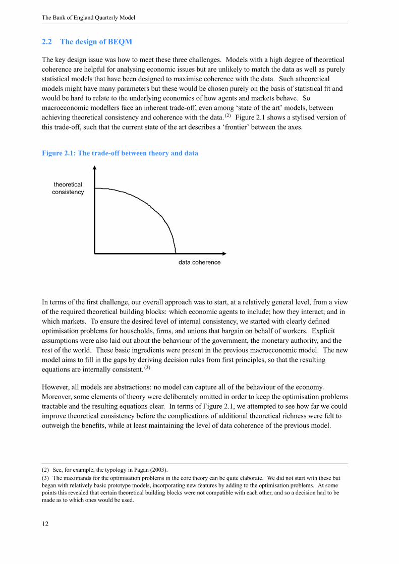
The key design issue was how to meet these three challenges. Models with a high degree of theoreticalcoherence are helpful for analysing economic issues but are unlikely to match the data as well as purelystatistical models that have been designed to maximise coherence with the data. Such atheoreticalmodels might have many parameters but these would be chosen purely on the basis of statistical fit andwould be hard to relate to the underlying economics of how agents and markets behave. Somacroeconomic modellers face an inherent trade-off, even among ‘state of the art’ models, betweenachieving theoretical consistency and coherence with the data. (2) Figure 2.1 shows a stylised version ofthis trade-off, such that the current state of the art describes a ‘frontier’ between the axes.
Figure 2.1: The trade-off between theory and data
theoretical consistency
data coherence
In terms of the first challenge, our overall approach was to start, at a relatively general level, from a viewof the required theoretical building blocks: which economic agents to include; how they interact; and inwhich markets. To ensure the desired level of internal consistency, we started with clearly definedoptimisation problems for households, firms, and unions that bargain on behalf of workers. Explicitassumptions were also laid out about the behaviour of the government, the monetary authority, and therest of the world. These basic ingredients were present in the previous macroeconomic model. The newmodel aims to fill in the gaps by deriving decision rules from first principles, so that the resultingequations are internally consistent. (3)
However, all models are abstractions: no model can capture all of the behaviour of the economy.Moreover, some elements of theory were deliberately omitted in order to keep the optimisation problemstractable and the resulting equations clear. In terms of Figure 2.1, we attempted to see how far we couldimprove theoretical consistency before the complications of additional theoretical richness were felt tooutweigh the benefits, while at least maintaining the level of data coherence of the previous model.
(2) See, for example, the typology in Pagan (2003).(3) The maximands for the optimisation problems in the core theory can be quite elaborate. We did not start with these butbegan with relatively basic prototype models, incorporating new features by adding to the optimisation problems. At somepoints this revealed that certain theoretical building blocks were not compatible with each other, and so a decision had to bemade as to which ones would be used.
12

Project motivation and model design
The sort of tightly specified structural model that this process delivers is a useful device for thinkingabout the transmission of shocks and policy, and the identification of different economic stories.However, such a model would probably have some difficulty in matching the data fully, because it wouldalways be missing some potentially important economic elements. Typically, in much of the academicliterature over the past 25 years, models have been designed to answer a specific question and cantherefore be focused on specific issues. In our case, however, the model is intended to be used as ageneral-purpose vehicle for policy analysis and forecasting, and we cannot neatly restrict the range ofeconomic issues that the model will face. Moreover, the ultimate users – policymakers on the MPC –must have confidence that the model is able to match general features of the UK economy and itsresponse to shocks, even if some of this behaviour is difficult to model structurally.
One approach to matching movements in the data, commonly used for macroeconomic models, is totreat the theory as a guide to the economic variables that appear in econometric regressions. (4) If a strictapproach is taken to deriving a reduced-form equation from theory, then the equation parameters will becombinations of the deep parameters from the structural decision rules. If cross-equation restrictionswere not strictly enforced, the linkages implicit in the original specifications would be weakened. Thiswould be problematic for our purposes, because so many of the forecast issues and risks revolve aroundcompeting structural stories, and we need to be able to trace their different effects through the model.These are not just variations in exogenous effects, such as assumptions for future world trade, but also inhow the economy responds to those effects. (5)
An alternative approach could be to retain the structural specifications derived from the optimisationproblems and to add extra, ad hoc components. But it is not clear where to place ad hoc elements in amicro-founded simultaneous system. Indeed, experiments along these lines confirmed that it would beeasy to create a system that generated unpredictable results and that might not even solve. To reap fullbenefit from a structural system, any additional elements should be worked through consistently fromthe original optimisation problem, which could risk making the model large and intractable.
To secure the benefits of the new model, our approach was to build the model in two distinct parts: atheoretical ‘core’ model, and ‘non-core’ equations that include additional variables and dynamics notmodelled formally in the core. When used together, these two parts form the full model that is the actualplatform used for producing forecast paths and allows the direct application of judgement.
The theoretical core is a structural model, containing a set of decision rules derived from first principlesand an associated set of consistency conditions, such as accounting constraints and stock-flow identities.It could be thought of as a dynamic general equilibrium model in which adjustment costs and otherfrictions are modelled explicitly. The decision rules are dynamic and are derived from the assumptionsthat agents act to maximise forward-looking objective functions according to dynamic constraints. (6) Itdescribes how we would expect changes in exogenous forces to work their way through the modeleconomy. A change to a given structural parameter would usually feed into many different decisionrules and would therefore affect how the system responds to shocks. The paths from this core model aretreated as starting points for the final forecast paths.
(4) See, for example, the programme laid out in Fair (1993) and (1994).(5) For example, the responses of the economy if goods markets were more or less competitive are well defined whereparameters for demand elasticities are identified throughout the system. But with reduced forms, the answer is often buried inthe constants and (quasi-) elasticities of the system. An expert user could make use of intercept adjustments, but this wouldtake some skill and time, which is not ideal when a large number of economic issues and uncertainties must be processedquickly.(6) For example, consumers are assumed to maximise expected lifetime utility subject to the constraint that their assets evolveaccording to a period-by-period budget constraint.
13

The Bank of England Quarterly Model
The full forecast model supplements the paths from the theoretical core with a statistical model of thediscrepancy between historical outturns and the paths generated by the core model. We supplement thecore theory for two reasons. First we might allow for different dynamics, such as more persistence thanthe theory implies. Second, we might allow for influences from variables that proxy for missing effects,such as credit channel effects and confidence effects through the business cycle. The only restriction onthe structure of ad hoc non-core equations is that the projected path for a given variable should alwaysconverge to the long-run equilibrium imposed by the core theory. This forecasting model is strictlyautoregressive, so that judgement (7) can be used to modify paths in a predictable way, which would bemore difficult within the structural core model. This is an important feature, allowing us to impose theCommittee’s judgements, using off-model information.
Actual forecast paths are thus combinations of three types of information:
• theoretical insight from the structural core model;• data-driven evidence on historical correlations of endogenous variables with other factors,especially those that are not formally accounted for in the structural core; and
• a direct application of judgement, informed by other models and staff expertise.
A key forecast question is how much weight these different contributions should carry in deriving thefinal forecast path.
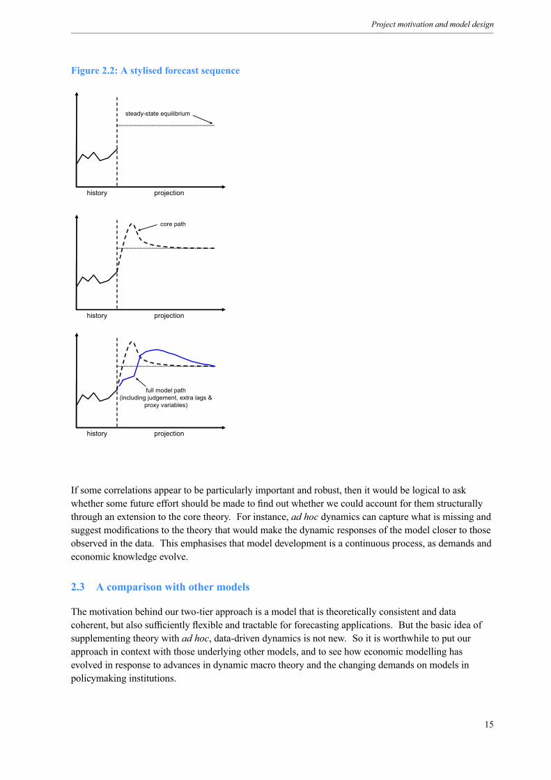
The profile for a given endogenous variable is built up from the core model and supplemented in the fullmodel by additional variables, dynamics or judgement, as illustrated in the stylised sequence below andin Figure 2.2: (8)
• given values for the exogenous variables, a steady-state version of the core model determines asustainable long-run equilibrium value;
• the core model indicates a path that converges from the current starting point to the long-run levelthat is consistent with the decision rules and constraints in the core theory; and
• in the full model, the path might have additional lags or proxy variables added, or judgementapplied. (9)
While this process allows a relatively free modification of the original path for a given endogenousvariable, the system still preserves accounting identities and stock-flow relations, so there are no ‘freelunches’ allowed by the application of judgement (the details of the application of this approach arediscussed in Chapter 4).
(7) These ‘addfactors’ are additional exogenous elements on the right-hand sides of equations. They are set to zero in the longrun, but can take various values to affect the path of a left-hand side variable. For example, suppose we have a system of theform:
y1t = a1 · y1t−1 + e1ty2t = a2 · y1t + e2t
A ‘type 1’ fix on y2t would be where we use e2t to achieve a desired path for y2t . For a ‘type 2’ fix, we would use e1t to affecty1t and therefore y2t .(8) For simplicity, the illustration is as if stationary and abstracts from trend growth.(9) This representation is very stylised; in practice, judgement might be applied to the long run (for instance, by changing coremodel parameters) as well as the short run.
14
Project motivation and model design
Figure 2.2: A stylised forecast sequence
history projection
history projection
steady-state equilibrium
core path
history projection
full model path(including judgement, extra lags &
proxy variables)
If some correlations appear to be particularly important and robust, then it would be logical to askwhether some future effort should be made to find out whether we could account for them structurallythrough an extension to the core theory. For instance, ad hoc dynamics can capture what is missing andsuggest modifications to the theory that would make the dynamic responses of the model closer to thoseobserved in the data. This emphasises that model development is a continuous process, as demands andeconomic knowledge evolve.
2.3 A comparison with other models
The motivation behind our two-tier approach is a model that is theoretically consistent and datacoherent, but also sufficiently flexible and tractable for forecasting applications. But the basic idea ofsupplementing theory with ad hoc, data-driven dynamics is not new. So it is worthwhile to put ourapproach in context with those underlying other models, and to see how economic modelling hasevolved in response to advances in dynamic macro theory and the changing demands on models inpolicymaking institutions.
15

The Bank of England Quarterly Model
There has been a long UK tradition associated with cointegration-based econometrics, which has beenvery influential in macromodelling. This approach uses theory to posit the existence of long-runrelations, which would be incorporated into the model if validated on statistical grounds. Examples ofthis approach include Hall and Henry (1987) and, to some extent, the Bank of England’s earlier MTMMmodel, which in broad terms is a large, restricted Vector Error-Correction Model (VECM). Thisapproach puts less emphasis on some aspects of theory, insofar as short-run dynamics are largely ‘datadriven’, and long-run relations implied by theory have to be confirmed by empirical work. For example,the modeller would not insist that the model has a balanced-growth equilibrium, but instead would testwhether the cointegrating relation implied by this was present in the data. (10) Similarly, the existence offorward-looking expectations and susceptibility to the Lucas critique are hypotheses to be tested. (11)
In the 1980s, a generation of UK macro models emerged that attempted to respond to the Lucas critiquedirectly with the use of rational expectations econometrics. (12), (13) These models typically placed astrong emphasis on consistency conditions such as stock-flow relations. (14) A typical approach wouldbe to take an equilibrium condition derived under the assumption of rational expectations and estimatethe parameters using some form of instrumental variables. For example, a consumption function mightbe used as the starting point for a regression of current consumption on leads of consumption, lags, andwealth terms. A good example of such an approach is the NIDEM model produced by the NationalInstitute of Economic and Social Research. (15) Such an approach effectively allows the model-builder totest directly the coherence of the theoretical relation against the data. The equations are nonetheless stillreduced form, with cross-equation restrictions enforced to varying degrees. (16) Because of this, some adhoc measures would be necessary if some technical features, such as a long-run balanced-growthsolution, were required. (17), (18)
In terms of models actively used by policy institutions to support forecasts and policy analysis, there hasbeen a steady shift towards models that place greater emphasis on theoretical consistency. (19), (20) Forexample, the Bank of Canada shifted from the RDXF model to the QPM in the early 1990s, and theBoard of Governors of the Federal Reserve moved from the MPS to the FRB/US model. The QPMmodel placed more weight on theoretically plausible parameter values than on direct econometric
(10)See Doornik and Hendry (1994) for an example of this approach.(11)See, for example, Favero and Hendry (1992).(12)An outstanding early example was the work on the Liverpool model (Minford (1980)). Subsequent work included that atthe National Institute for Economic and Social Research (Hall and Henry (1985) and (1987)), the LBS model (Budd et al(1984) and Dinenis et al (1989)), the City University CUBS model, and, more recently, COMPACT (Darby et al (1999)). SeeWallis and Whitley (1991) for a commentary.(13)Wallis (1980) was an early investigation of the consequences of rational expectations for macroeconometric specifications.(14)The importance of consistency conditions was emphasised in pioneering work on optimal control in forward-lookingmodels – see, for example, Holly and Zarrop (1983) and Holly (1986).(15)This has several vintages; see Wren-Lewis (1989) for an example.(16) In this sense, these models can be interpreted as overidentified VARs; typical identifying assumptions that would bemaintained are homogeneity restrictions.(17)For example, in the case of the NIESR model referred to here, a stable net foreign asset position was ensured byconfiguring the fiscal rule so that the government effectively took the role of ensuring an economy-wide savings equilibrium.(18)Extensive comparisons of UK macro models have been conducted, especially by the ESRC Macroeconomic ModellingBureau from 1983 to 1999. See Andrews et al (1984), (1985), (1986); Fisher et al (1987), (1989), (1990); and Church et al(1991), (1993), (1995), (1997), (2000).(19)This was facilitated by advances in solution algorithms that made simulations with large-scale non-linear models withmodel-consistent expectations feasible; see, for example, Fisher, Holly and Hughes-Hallett (1986).(20)Some, however, would regard existing macroeconometric forecasting models as well within the possible frontier, payingless attention to issues of simultaneity and cross-equation restrictions than would have been the case in macroeconomic modelsof the 1960s; see Sims (2002). Indeed, the Liverpool model of the late 1970s was theoretically very strict by today’s standards.
16

Project motivation and model design
estimates. (21) It uses a calibrated theoretical model to pin down a set of steady-state attractors forerror-correcting relationships. (22) Dynamics are driven by assuming, on a partial equilibrium basis, thatthere are adjustment costs between current and long-run target levels for a variable. (23)
In the FRB/US model, theory is used to inform long-run relationships, and some of these are forwardlooking, such as human wealth. (24) Dynamics are assumed to be driven by generalised adjustment costs,and the existence of higher orders of adjustment costs introduces a role for forward expectations. (25)
The full model is a mixture of structural relations implied by a partial equilibrium treatment of theory(such as the decision rule for aggregate consumption) and some reduced-form relations (such as thetrade block, which employs error-correcting relationships.)
A similar transition was made by the International Monetary Fund (IMF) with the shift to the Mark IIIvintage of the MULTIMOD multi-country model. Since MULTIMOD was intended to be used more asa simulation model rather than a direct forecasting tool, several of the changes which were implementedin the Mark III version arose from the need to enrich its theoretical structure, so that it could deal withnew macroeconomic issues such as current account imbalances. (26) As with the QPM, a steady-statemodel enforced necessary terminal conditions. (27)
Other central banks have followed with variations of their own. In 1997, the Reserve Bank of NewZealand moved away from spreadsheet-based forecasting to a formal model, FPS, that drew on theexperience with QPM. (28) That model can be viewed as a forward-looking IS/LM system with adisaggregated IS curve. The difference between ad hoc calibrated dynamics and ‘equilibrium’ dynamicsfor real variables defines an output gap, which drives the nominal side through a Phillips curve. Work atthe Bank of Japan has pursued and extended this approach, (29) and a variant of the QPM model has beenused by the Sveriges Riksbank in the form of the RIKSMOD model.
Recent work at several institutions indicates that this process may go several steps further. Projects atthe Board of Governors of the Federal Reserve and the Bank of Canada are now under way to exploremodels with theory-based dynamics as well as long-run properties. Work on the GEM model at the IMFand the EDGE and AINO models at Bank of Finland can also be seen in this way.
In the case of BEQM, the model is split into two tiers – the structural model is kept intact, with noattempt to introduce ad hoc components directly; forecast paths are constructed as a weighted average ofpaths from the structural model and paths driven by statistically robust correlations, together withapplication of policymakers’ judgements. This approach reflects the nature of the forecast process at theBank of England. As much as possible, an attempt is made to understand the forces at work on themacroeconomy in terms of fundamental economic drivers and constraints, which are articulated in the
(21)For example, Coletti et al (1996) comment that ‘there had been a systematic tendency towards over-fitting equations andtoo little attention to capturing the underlying economics. It was concluded that the model should focus on capturing thefundamental economics necessary to describe how the macro economy functions, and, in particular, how policy works’ (page14).(22)See Black et al (1994).(23)See Coletti et al (1996).(24)See Brayton and Tinsley (1996).(25)See Kozicki and Tinsley (1999).(26)See Laxton et al (1998).(27)This was to compute the terminal conditions for the forward-looking variables in the model. It also enabled users to relaxthe assumption of earlier vintages that current accounts have to balance in the long run, which enabled better investigation ofsustainability issues.(28)See Black et al (1997) and Hunt et al (2000).(29)See Fujiwara et al (2004).
17

The Bank of England Quarterly Model
core model. But our understanding of the macroeconomy is imperfect, so it is logical to ask whethersome weight should be given to correlations that are robust in the data but might be difficult to explain ormodel in a fully structural way. Other, more specialised models can provide insight on specific issues orvariables, as can sectoral expertise available within the Bank. These suggest instances when judgementcan usefully be applied.
2.4 Summary
This chapter discusses some of the factors behind the design of BEQM. The main motivation fordeveloping a new model was to improve theoretical consistency and clarity. A number of specificrequirements stem from its role in helping to produce the MPC’s quarterly economic forecast and inanalysing the economic issues underlying the forecasts, together with associated risks and uncertainties.This meant that we want a model that is rich enough to be able to analyse a wide range of economicissues; that can match the observed data; and that is reliable and robust under the pressures of a real-timeforecasting round – including the ability to impose judgement and conditioning paths.
Our approach was to build a model with two distinct parts. We start with a tightly specified theoreticalcore model, containing dynamic decision rules derived from the solution of dynamic optimisationproblems. We supplement this with non-core equations that include additional lags and variables tomatch dynamics that are not modelled formally in the core. These equations also allow the impositionof judgement based on ‘off-model’ information. The final forecast path can be thought of as acombination of theoretical insight from the structural core model; additional variables and dynamicsfrom the non-core; and direct application of judgement.
Finally, we put BEQM into historical context by discussing advances in macroeconomic model buildingover the past 25 years. Over time, greater emphasis has been placed on theoretical consistency, andadvances in computing power have allowed more complex models to be employed.
18
Project motivation and model design
Box 1: Some recent developments towards hybrid structural models
Substantial effort in recent years has been directed towards ‘hybrid’ models, which preserverelatively strong, theoretically derived identification structures but nonetheless fit the dataaccording to some well defined statistical metric. Some of this work can be thought of as comingfrom a relatively atheoretic perspective, such as the Vector Auto Regression (VAR) literature; otherwork takes theoretically tight models, such as from the Dynamic Stochastic General Equilibrium(DSGE) literature, as a starting point, and asks what has to be done to make such models fit thedata. The attempt at convergence is logical, because both approaches yield a compactautoregressive form that can be assessed against the data.
In the VAR literature more and more use has been made of long-run (and even short-run)identifying restrictions; for example, Leeper and Zha (2001) aimed to produce a VAR model that is‘useful’ for monetary policy analysis. A small number of papers have attempted to exploit thedata-matching properties of VARs together with the story-telling advantages of structural models.McKibbin, Pagan and Robertson (1998), for example, start with a VAR to produce a hybrid modelthat retains the very short-run properties of the VAR, but is designed to match some of the featuresof a calibrated structural model. There is now a substantial literature that assesses DSGE modelsagainst their corresponding VARs. (a)
In a conventional DSGE approach, first-order approximations to the decision rules derived fromdynamic optimisation problems are evaluated at a deterministic steady state. The useful ‘trick’ ofthe DSGE approach that makes the solution of these models tractable is to assume that theexogenous variables follow a simple autoregressive process. Given this assumption, the rationalexpectations of future variables can be derived as functions of current states of the world, leadingto a backward-looking representation of the dynamic solution to the model. The generic statespace representation of these models will have the form
st = Ast−1 + But (1)yt = Cst (2)
where s is a vector of states of the world, u is a vector of shocks and y is a vector of endogenousvariables. A, B, and C are conformable matrices, where the elements are combinations ofstructural parameters. Usually y will be larger-dimensioned than s: given knowledge about theevolution of a relatively limited number of states of the world (eg capital stock, previous levels ofconsumption), we make inferences about a wide range of variables (such as output, wage rates,employment, and asset prices).
In its state-space form, the model can be run recursively against the historical data and predictionerrors can be extracted from the difference between predicted and actual y. Notionally at least,these errors could be used to evaluate a likelihood function. A problem arises when applying thisto the canonical Ramsey mode, which has a single stochastic process (technology), in that thecovariance matrix is singular. But if we augment the range of extrinsic dynamics so that there is astochastic process for each endogenous variable, then exact maximum likelihood is possible.
(a) See, for example, Canova, Finn, and Pagan (1994).
19
The Bank of England Quarterly Model
Hence, in recent years we have seen papers (eg Hansen (1985)) in which parameters that wouldpreviously have been held fixed are allowed to vary over time. For example, instead of aconventional household maximisation problem with fixed time preference and utility weights onconsumption (c) and leisure (the proportion of available time not spent working, 1− h):
max Et∞
i=0β i {log ct+i + A log (1− ht+i )}
we could now specify the problem as
max Et∞
i=0ϕt+i {log ct+i + At log (1− ht+i )}
ϕ t+i = (1− ρϕ)ϕ + ρϕϕ t+i−1 + εϕt+i 0 ≤ ρϕ < 1At+i = (1− ρ A) A + ρ AAt+i−1 + εAt+i 0 ≤ ρA < 1
Other extensions include capital-specific and labour-specific effectiveness processes, time-varyinginvestment efficiency, and policy shocks. One would add shock processes to the optimisationproblem until there is a stochastic process for each endogenous variable. Then estimation ofparameters is possible using the Kalman filter to extract prediction errors to be assessed using thelikelihood function. A recent example of adding shock processes to the optimisation problem canbe found in Smets and Wouters (2003a) A potential disadvantage with this type of model is thatits projections are driven by a large set of unobservable shocks, some of which might be regardedas arbitrary and difficult to interpret.
A Bayesian rather than classical approach to this problem can also be taken. One implementationis to use the recursive state-space form of the theoretical model to generate artificial data. Theparameters of the system can then be estimated using a pseudo-sample that combines actual withartificial data. The higher the proportion of artificial data used in the pseudo-sample, the higherthe weight on theoretical priors. Bayesian ‘shrinkage’ procedures can be used to determine theoptimal weight on theory and data. For example, Ingram and Whiteman (1994) showed that usingpriors and cross-equation restrictions from a Real Business Cycle (RBC) model allowed for aconsiderable improvement in the performance of a VAR, compared with the unrestricted VARform and a VAR using the Minnesota (random walk) prior. Recent implementations include DelNegro and Schorfheide (2004).
In different contexts, it is conventional to refer to (2) as a measurement equation, reflecting theassumption that the linear transforms of state values in Cs will only be imperfect approximationsto observed data in y. For example, we do not observe ‘output’ or ‘marginal product of labour’directly, but have constructed measures such as ‘private sector value added at current prices’ and‘unit labour costs’.
Sargent (1989) exploited this structure to deal with issues about data mismeasurement. In hisschema, we would have (1) as before, but (2) would be augmented to include error terms:
yt = Cst + etet = Det−1 + ξ t
20

Project motivation and model design
As the error terms are assumed to represent measurement error, they are orthogonal: D and cov(et)are assumed to be diagonal. However, Ireland (2004) suggests that we interpret the errors as adhoc processes to make up for the misspecification of the model in fitting the data to y, by allowingD and cov(et) to have non-zero off-diagonal elements. In this case, the errors are not orthogonaland will be correlated with the elements in s in almost all cases. In other words, the theoreticalmodel embodied in the relations (1) and (2) is assumed to be wrong, and so the question, in thespirit of Watson (1993), is what needs to be done in e in order to match the data in y.
While much progress has been made in terms of numerical methods, these sorts of techniques haveonly been applied to relatively compact systems where the interpretation of the correspondingreduced-form VAR representation is relatively straightforward. It is not yet clear how the addedunobservable extrinsic dynamics in these models should be interpreted in terms of the demands ofa forecast process and the need to understand the underlying economic drivers of the forecast.Nonetheless, this literature holds some promise in terms of reconciling demands for theoreticalconsistency with coherence with the data.
21


Chapter 3 The core theory
This chapter summarises the core theory, describing the main building blocks, with attention to theinteractions between agents and the key assumptions. An overview of the core theory (Section 3.1) isfollowed in Section 3.2 by discussion of the objectives and constraints of the key agents: households,firms, the government, the monetary authority and the rest of the world. Section 3.3 describes how theseagents interact in markets for goods, labour and capital. This is followed in Section 3.4 by an account ofthe nominal side, including money market equilibrium and the price level, nominal wages and prices,inflation, and the monetary transmission mechanism. Section 3.5 deals with real trend growth, followedby a summary of the chapter in Section 3.6.
3.1 Overview
We can think of the core theory as an organising framework for analysing the economy. It should helpus tease apart competing explanations of what we observe in the data, by reminding us of the differentimplications of each story. To do this, the theory in the core model needs to be sufficiently rich andgeneral to handle a wide range of issues, while at the same time being compact enough to be tractable,reliable and clear. In order to secure the level of internal consistency that we want from the core model,we take an optimisation-based approach that begins with clear statements about how the key agents actin the face of constraints.
To this end, we wanted the theory to describe an economy where:
• households receive wage income and transfers from both firms and the government, and returnsfrom assets, while paying for a bundle of domestically produced and imported consumption goods,making investments in housing and financial assets (shares, bonds and money) and paying taxes tothe government;
• domestic firms receive income from selling final goods in domestic and overseas markets, whilepaying taxes and (potentially) receiving transfers from the government, paying for factor inputs ofdomestically sourced capital goods, imported capital goods, and labour. They finance this activitythrough the issue of equity and debt, and accumulating and decumulating inventories;
• the government generates revenue from taxes, new debt issuance and seigniorage, while purchasinggoods and services from firms and labour services from households, and servicing existing debt;
• the monetary authority sets a short-term nominal interest rate in order to achieve an inflation targetand, consequently, provides nominal stability; and
• the rest of the world provides capital, goods and services demanded by the domestic economy, andis a potential market for domestic production.
The core theory contains explicit decision rules and constraints that specify how these key agentsinteract with each other in markets for capital, financial assets, goods and labour. The treatment of theagents differs quite substantially: decision rules for households and firms arise out of explicitoptimisation problems, while the rest of the world is exogenous. The monetary authority and thegovernment are given simple reaction functions that specify policy targets and an endogenousinstrument. This description of the core model economy is illustrated in Figure 3.1.
23

The Bank of England Quarterly Model
Figure 3.1: Key agents in the model macroeconomy
Households Firms
GovernmentMonetary authority
Domestic economy World economy
maximise utility subject to budget constraint
maximise profits subject to demand and
technology
reaction function to specify nominal instrument in reaction to deviations
from nominal anchor
reaction function to specify fiscal instrument to ensure
debt sustainability
Rest of world
assumed to be 'large' with respect to
domestic economy
Likewise, there are some important differences in the assumptions made for various markets. Wewanted the theory to describe an economy in which:• goods markets are monopolistically competitive, leading to profits and an ability for firms to chargenon-competitive sticky prices, which clear all of domestic production to satisfy demands (net ofimports) for consumption, investment, changes in inventories, government spending and exports;
• the labour market equilibrium is not perfectly competitive. Firms and unions bargain over wagelevels which generate unemployment, given private sector and public sector labour demand, laboursupply and wage curves; and
• asset market prices reflect standard no-arbitrage conditions, with (net) assets owned by domestichouseholds and overseas residents, and long-run real interest rates are pinned down by worldconditions.
This broad view of the economy is unchanged from the previous macro model. Indeed, many of thetheoretical building blocks of the previous model have been used here, including the paradigm of asingle, constant returns to scale production function on the supply side; the union bargaining frameworkfor the labour market; and the same small open economy assumptions.
The key difference here lies in the implementation, where we have now been more explicit about whatmotivates the agents, their constraints, and the characteristics of the markets in which they interact. Thisconsistent approach leads to a number of technical features: a well defined, balanced-growth steadystate; consistent stock-flow accounting; binding budget constraints; an explicit treatment of expectations;and the potential for endogenous policy reaction.
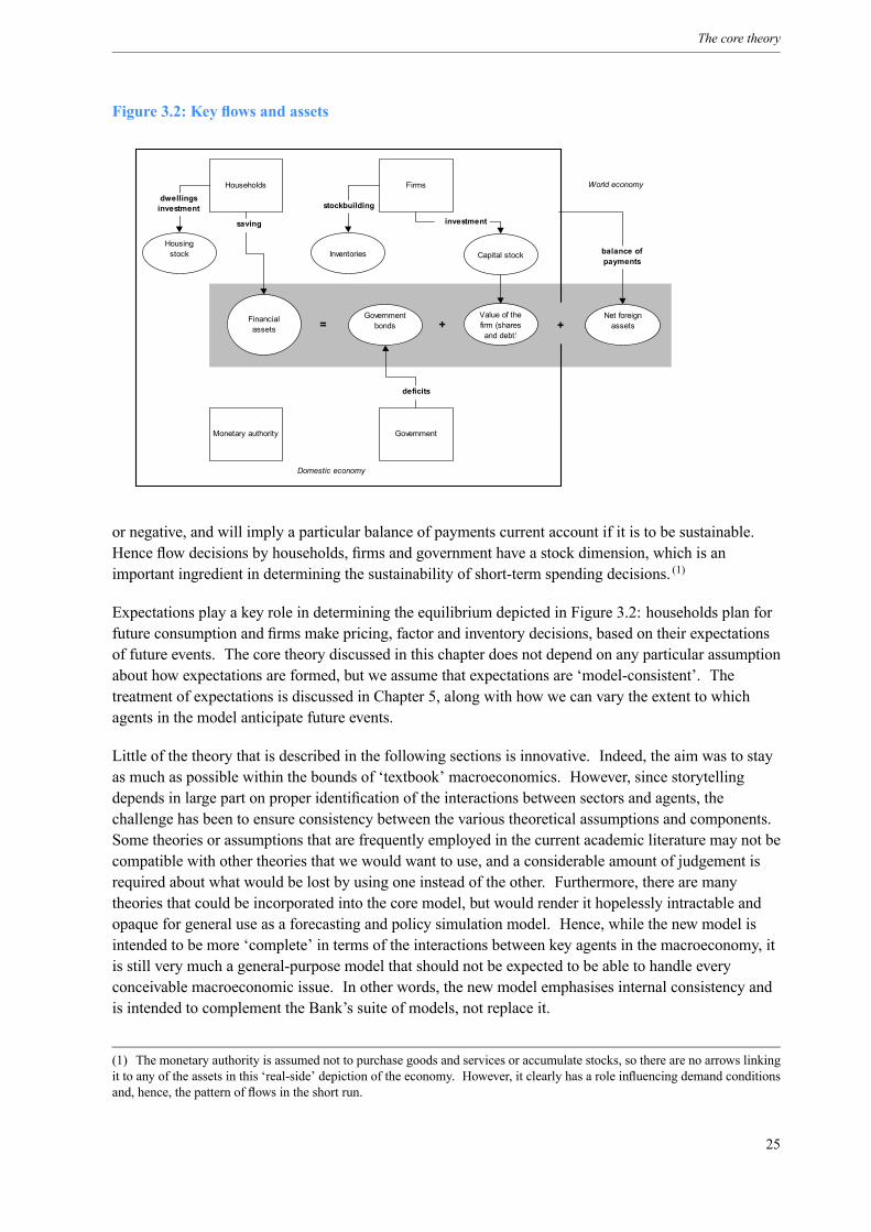
Figure 3.2 shows how agents are linked by expenditure flows and the accumulation of physical andfinancial assets. The government is bound by a budget constraint, so that deficits cumulate intogovernment debt. Firms cumulate physical stocks of inventories and capital goods, and must financetheir activities, so accumulating liabilities of debt and equity. The key linkage is that these liabilitiesmust ultimately be held as assets by households or the rest of the world. Households’ decisions abouthow much to consume – reflecting their desired level of total financial wealth – will ultimately bereflected in the level of net foreign assets that the UK economy holds. This net balance can be positive
24
The core theory
Figure 3.2: Key flows and assets
Households Firms
GovernmentMonetary authority
Financial assets
Government bonds
Value of the firm (shares and debt)
Housing stock Capital stock
Net foreign assets+
saving
deficits
investment
Domestic economy
World economy
balance of payments
Inventories
= +
dwellings investment stockbuilding
or negative, and will imply a particular balance of payments current account if it is to be sustainable.Hence flow decisions by households, firms and government have a stock dimension, which is animportant ingredient in determining the sustainability of short-term spending decisions. (1)
Expectations play a key role in determining the equilibrium depicted in Figure 3.2: households plan forfuture consumption and firms make pricing, factor and inventory decisions, based on their expectationsof future events. The core theory discussed in this chapter does not depend on any particular assumptionabout how expectations are formed, but we assume that expectations are ‘model-consistent’. Thetreatment of expectations is discussed in Chapter 5, along with how we can vary the extent to whichagents in the model anticipate future events.
Little of the theory that is described in the following sections is innovative. Indeed, the aim was to stayas much as possible within the bounds of ‘textbook’ macroeconomics. However, since storytellingdepends in large part on proper identification of the interactions between sectors and agents, thechallenge has been to ensure consistency between the various theoretical assumptions and components.Some theories or assumptions that are frequently employed in the current academic literature may not becompatible with other theories that we would want to use, and a considerable amount of judgement isrequired about what would be lost by using one instead of the other. Furthermore, there are manytheories that could be incorporated into the core model, but would render it hopelessly intractable andopaque for general use as a forecasting and policy simulation model. Hence, while the new model isintended to be more ‘complete’ in terms of the interactions between key agents in the macroeconomy, itis still very much a general-purpose model that should not be expected to be able to handle everyconceivable macroeconomic issue. In other words, the new model emphasises internal consistency andis intended to complement the Bank’s suite of models, not replace it.
(1) The monetary authority is assumed not to purchase goods and services or accumulate stocks, so there are no arrows linkingit to any of the assets in this ‘real-side’ depiction of the economy. However, it clearly has a role influencing demand conditionsand, hence, the pattern of flows in the short run.
25
The Bank of England Quarterly Model
3.2 Characterisation of the agents
3.2.1 Households
Households are important because their choice of a desired level of financial assets, given the supply ofdomestic assets, determines the long-run equilibrium for sustainable consumption, net foreign assets andthe trade balance. A key issue for the theory of the household is how this equilibrium is determined.We also want the household theory to account for the demand for real money balances, the demand forhousing, and the split of consumption between domestically produced and imported goods. Further, wewant some control over the short-run dynamic convergence to long-run equilibrium for these demands.Our approach starts with a standard utility-maximisation problem, but instead of dealing with a singlerepresentative agent, we aggregate individual decision rules to derive total demands for consumption,housing and money.
We consider first the optimisation problem for individuals: they aim to maximise lifetime utility subjectto their expected lifetime resources. The first source of utility is consumption of domestically producedand imported non-durable goods, and services from housing (which we treat as a very durable good).Individuals also gain utility from holding real money balances, which in this context can be thought of asan implicit requirement for cash for transactions. (2) Individuals also form habits and value leisuretime. (3) To keep the model as simple as possible, we abstract from public finance issues that might berelevant for a fiscal authority, so public goods do not enter utility and government consumption andinvestment do not benefit households directly. (4) Turning to income, households rent their labour tofirms or the government and receive wages in return (see Section 3.3.2). Households are also assumedto receive certain transfers directly from firms (such as corporate pension contributions), as well astransfers from the government (such as government benefits). To smooth consumption, households canborrow and save using a range of financial assets, including government securities, corporate bonds,shares and foreign bonds. (5)
A commonly used assumption is that of a representative agent who lives for ever, which would implythat the level of net foreign assets is not pinned down to a particular long-run equilibrium level. (6) Ourassumption that the domestic economy is small in relation to international capital markets implies that aninfinitely lived domestic agent would be able to borrow an infinite amount and pay it off in the indefinitefuture. If such domestic agents were ‘impatient’ relative to the rest of the world, domestic householdswould accumulate an infinite amount of net foreign debt; if domestic agents were more ‘patient’ than therest of the world, the domestic economy would acquire all the assets from the rest of world. (7) Thiswould violate the assumption that the domestic economy is small in relation to international capitalmarkets and is incompatible with our basic requirement that the interaction of agents in the modeldetermines a long-run sustainable equilibrium for consumption, net foreign assets and trade.
(2) Money is assumed to provide services that mitigate transactions frictions. Real money balances enter the utility functionadditively.(3) Technically, this is not implemented in the same way as conventional direct leisure in lifetime utility, and does not affectthe marginal propensity to consume. ‘Unions’ are assumed to bargain on behalf of workers – see Section 3.3.2.(4) As long as public goods enter utility additively, they would not affect consumption decisions in any case.(5) See Box 2 on page 30 for the consumer’s maximisation problem.(6) This model does have growth – see Section 3.5 – so that in what follows ‘consumption’ refers to the consumption-outputratio.(7) That is, if β (1+ r) > 1, where β is the individual’s discount factor and r a real return on assets, then consumption willsteadily grow and foreign assets will fall. Conversely, if β (1+ r) < 1 then consumption will steadily fall and foreign assetswill rise. See Chapter 3 of Barro and Sala-i-Martin (1995).
26
The core theory
There are several modifications to the infinitely lived representative agent model that renderconsumption stationary. (8) However, these methods typically imply that one of consumption, netforeign assets or the current account has to return to a predetermined value, rather than each reactingendogenously to shocks, as we would like. In addition, they usually require that the household rate oftime preference equals a constant foreign real interest rate, which is an unattractive feature in our casebecause movements in foreign real interest rates can be a key forecast issue. Further, these modelstypically preclude discussions of ‘pure’ wealth effects, which would further restrict the ability of themodel to analyse forecast issues. (9)
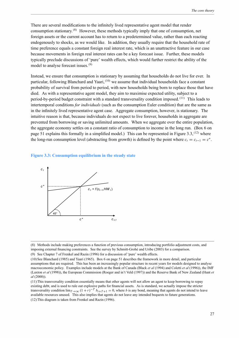
Instead, we ensure that consumption is stationary by assuming that households do not live for ever. Inparticular, following Blanchard and Yaari, (10) we assume that individual households face a constantprobability of survival from period to period, with new households being born to replace those that havedied. As with a representative agent model, they aim to maximise expected utility, subject to aperiod-by-period budget constraint with a standard transversality condition imposed. (11) This leads tointertemporal conditions for individuals (such as the consumption Euler condition) that are the same asin the infinitely lived representative agent case. Aggregate consumption, however, is stationary. Theintuitive reason is that, because individuals do not expect to live forever, households in aggregate areprevented from borrowing or saving unlimited amounts. When we aggregate over the entire population,the aggregate economy settles on a constant ratio of consumption to income in the long run. (Box 6 onpage 51 explains this formally in a simplified model.) This can be represented in Figure 3.3, (12) wherethe long-run consumption level (abstracting from growth) is defined by the point where ct = ct−1 = c∗.
Figure 3.3: Consumption equilibrium in the steady state
c t
c *c t = f (ct -1,HW t )
c * c t-1
45°
(8) Methods include making preferences a function of previous consumption, introducing portfolio adjustment costs, andimposing external financing constraints. See the survey by Schmitt-Grohé and Uribe (2003) for a comparison.(9) See Chapter 7 of Frenkel and Razin (1996) for a discussion of ‘pure’ wealth effects.(10)See Blanchard (1985) and Yaari (1965). Box 6 on page 51 describes the framework in more detail, and particularassumptions that are required. This has been an increasingly popular structure in recent years for models designed to analysemacroeconomic policy. Examples include models at the Bank of Canada (Black et al (1994) and Coletti et al (1996)), the IMF(Laxton et al (1998)), the European Commission (Roeger and in’t Veld (1997)) and the Reserve Bank of New Zealand (Hunt etal (2000)).(11)This transversality condition essentially means that other agents will not allow an agent to keep borrowing to repayexisting debt, and is used to rule out explosive paths for financial assets. As is standard, we actually impose the strictertransversality condition limT→∞ (1+ r)−T bt+T+1 = 0, where b is any bond, meaning that agents do not intend to leaveavailable resources unused. This also implies that agents do not leave any intended bequests to future generations.(12)This diagram is taken from Frenkel and Razin (1996).
27
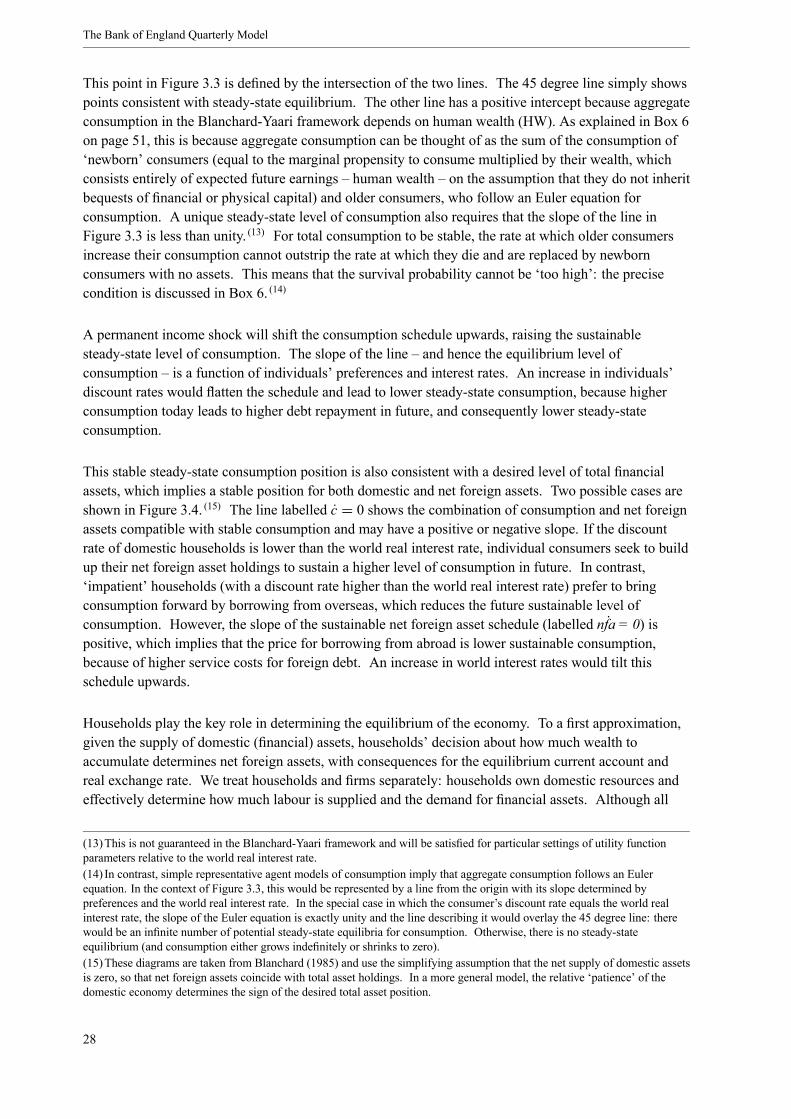
The Bank of England Quarterly Model
This point in Figure 3.3 is defined by the intersection of the two lines. The 45 degree line simply showspoints consistent with steady-state equilibrium. The other line has a positive intercept because aggregateconsumption in the Blanchard-Yaari framework depends on human wealth (HW). As explained in Box 6on page 51, this is because aggregate consumption can be thought of as the sum of the consumption of‘newborn’ consumers (equal to the marginal propensity to consume multiplied by their wealth, whichconsists entirely of expected future earnings – human wealth – on the assumption that they do not inheritbequests of financial or physical capital) and older consumers, who follow an Euler equation forconsumption. A unique steady-state level of consumption also requires that the slope of the line inFigure 3.3 is less than unity. (13) For total consumption to be stable, the rate at which older consumersincrease their consumption cannot outstrip the rate at which they die and are replaced by newbornconsumers with no assets. This means that the survival probability cannot be ‘too high’: the precisecondition is discussed in Box 6. (14)
A permanent income shock will shift the consumption schedule upwards, raising the sustainablesteady-state level of consumption. The slope of the line – and hence the equilibrium level ofconsumption – is a function of individuals’ preferences and interest rates. An increase in individuals’discount rates would flatten the schedule and lead to lower steady-state consumption, because higherconsumption today leads to higher debt repayment in future, and consequently lower steady-stateconsumption.
This stable steady-state consumption position is also consistent with a desired level of total financialassets, which implies a stable position for both domestic and net foreign assets. Two possible cases areshown in Figure 3.4. (15) The line labelled c = 0 shows the combination of consumption and net foreignassets compatible with stable consumption and may have a positive or negative slope. If the discountrate of domestic households is lower than the world real interest rate, individual consumers seek to buildup their net foreign asset holdings to sustain a higher level of consumption in future. In contrast,‘impatient’ households (with a discount rate higher than the world real interest rate) prefer to bringconsumption forward by borrowing from overseas, which reduces the future sustainable level ofconsumption. However, the slope of the sustainable net foreign asset schedule (labelled nfa = 0) ispositive, which implies that the price for borrowing from abroad is lower sustainable consumption,because of higher service costs for foreign debt. An increase in world interest rates would tilt thisschedule upwards.
Households play the key role in determining the equilibrium of the economy. To a first approximation,given the supply of domestic (financial) assets, households’ decision about how much wealth toaccumulate determines net foreign assets, with consequences for the equilibrium current account andreal exchange rate. We treat households and firms separately: households own domestic resources andeffectively determine how much labour is supplied and the demand for financial assets. Although all
(13)This is not guaranteed in the Blanchard-Yaari framework and will be satisfied for particular settings of utility functionparameters relative to the world real interest rate.(14) In contrast, simple representative agent models of consumption imply that aggregate consumption follows an Eulerequation. In the context of Figure 3.3, this would be represented by a line from the origin with its slope determined bypreferences and the world real interest rate. In the special case in which the consumer’s discount rate equals the world realinterest rate, the slope of the Euler equation is exactly unity and the line describing it would overlay the 45 degree line: therewould be an infinite number of potential steady-state equilibria for consumption. Otherwise, there is no steady-stateequilibrium (and consumption either grows indefinitely or shrinks to zero).(15)These diagrams are taken from Blanchard (1985) and use the simplifying assumption that the net supply of domestic assetsis zero, so that net foreign assets coincide with total asset holdings. In a more general model, the relative ‘patience’ of thedomestic economy determines the sign of the desired total asset position.
28
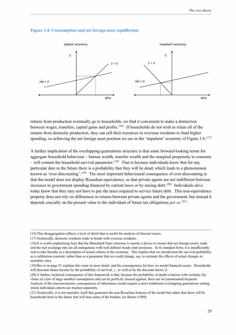
The core theory
Figure 3.4: Consumption and net foreign asset equilibrium
C
c = 0
NFA
nfa = 0
'patient' economy
C
c = 0
NFA
nfa = 0
'impatient' economy
.
.
.
.
returns from production eventually go to households, we find it convenient to make a distinctionbetween wages, transfers, capital gains and profits. (16) If households do not wish to retain all of thereturns from domestic production, they can sell their resources to overseas residents to fund higherspending, so achieving the net foreign asset position we see in the ‘impatient’ economy of Figure 3.4. (17)
A further implication of the overlapping-generations structure is that some forward-looking terms foraggregate household behaviour – human wealth, transfer wealth and the marginal propensity to consume– will contain the household survival parameter. (18) That is because individuals know that for anyparticular date in the future there is a probability that they will be dead, which leads to a phenomenonknown as ‘over-discounting’. (19) The most important behavioural consequence of over-discounting isthat the model does not display Ricardian equivalence, so that private agents are not indifferent betweenincreases in government spending financed by current taxes or by raising debt. (20) Individuals alivetoday know that they may not have to pay the taxes required to service future debt. This non-equivalenceproperty does not rely on differences in returns between private agents and the government, but instead itdepends crucially on the present value to the individual of future tax obligations per se. (21)
(16)This disaggregation reflects a level of detail that is useful for analysis of forecast issues.(17)Technically, domestic residents trade in bonds with overseas residents.(18) It is worth emphasising here that the Blanchard-Yaari structure is mainly a device to ensure that net foreign assets, tradeand the real exchange rate are all endogenous with well defined steady-state positions. In its standard form, it is insufficientlyrich to take literally as a description of actual cohorts in the economy. This implies that we should treat the survival probabilityas a calibration constant, rather than as a parameter that we could change, say, to estimate the effects of actual changes inmortality rates.(19)Box 6 on page 51 explains this issue in more detail, and the consequences for how we model financial assets. Householdswill discount future income by the probability of survival, γ , as well as by the discount factor, β.(20)A further, technical consequence of this framework is that, because the probability of death is known with certainty (byvirtue of a law of large numbers assumption) and can be perfectly insured against, there are no (unintended) bequests.Analysis of the macroeconomic consequences of inheritance would require a more traditional overlapping-generations setting,where individual cohorts are tracked separately.(21)Technically, it is not mortality itself that generates the non-Ricardian features of the model but rather that there will behouseholds born in the future that will bear some of the burden; see Buiter (1988).
29
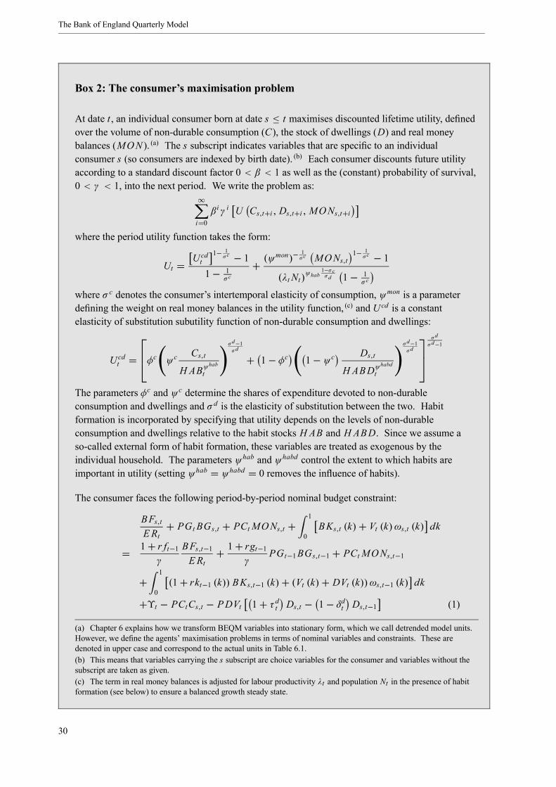
The Bank of England Quarterly Model
Box 2: The consumer’s maximisation problem
At date t , an individual consumer born at date s ≤ t maximises discounted lifetime utility, definedover the volume of non-durable consumption (C), the stock of dwellings (D) and real moneybalances (MON ). (a) The s subscript indicates variables that are specific to an individualconsumer s (so consumers are indexed by birth date). (b) Each consumer discounts future utilityaccording to a standard discount factor 0 < β < 1 as well as the (constant) probability of survival,0 < γ < 1, into the next period. We write the problem as:
∞
i=0β iγ i U Cs,t+i , Ds,t+i ,MONs,t+i
where the period utility function takes the form:
Ut = Ucdt1− 1
σ c − 11− 1
σ c
+ (ψmon)−
1σc MONs,t
1− 1σc − 1
(λt Nt)ψhab
1−σ cσd 1− 1
σ c
where σ c denotes the consumer’s intertemporal elasticity of consumption, ψmon is a parameterdefining the weight on real money balances in the utility function, (c) and Ucd is a constantelasticity of substitution subutility function of non-durable consumption and dwellings:
Ucdt =⎡⎢⎣φc ψc
Cs,tH ABψ
hab
t
σd−1σd
+ 1− φc 1− ψc Ds,tH ABDψ
habd
t
σd−1σd
⎤⎥⎦σdσd−1
The parameters φc and ψc determine the shares of expenditure devoted to non-durableconsumption and dwellings and σ d is the elasticity of substitution between the two. Habitformation is incorporated by specifying that utility depends on the levels of non-durableconsumption and dwellings relative to the habit stocks H AB and H ABD. Since we assume aso-called external form of habit formation, these variables are treated as exogenous by theindividual household. The parameters ψhab and ψhabd control the extent to which habits areimportant in utility (setting ψhab = ψhabd = 0 removes the influence of habits).
The consumer faces the following period-by-period nominal budget constraint:
BFs,tE Rt
+ PGt BGs,t + PCtMONs,t +1
0BKs,t (k)+ Vt (k) ωs,t (k) dk
= 1+ r ft−1γ
BFs,t−1ERt
+ 1+ rgt−1γ
PGt−1BGs,t−1 + PCtMONs,t−1
+1
0(1+ rkt−1 (k)) BKs,t−1 (k)+ (Vt (k)+ DVt (k)) ωs,t−1 (k) dk
+ϒt − PCtCs,t − PDVt 1+ τ dt Ds,t − 1− δdt Ds,t−1 (1)
(a) Chapter 6 explains how we transform BEQM variables into stationary form, which we call detrended model units.However, we define the agents’ maximisation problems in terms of nominal variables and constraints. These aredenoted in upper case and correspond to the actual units in Table 6.1.(b) This means that variables carrying the s subscript are choice variables for the consumer and variables without thesubscript are taken as given.(c) The term in real money balances is adjusted for labour productivity λt and population Nt in the presence of habitformation (see below) to ensure a balanced growth steady state.
30
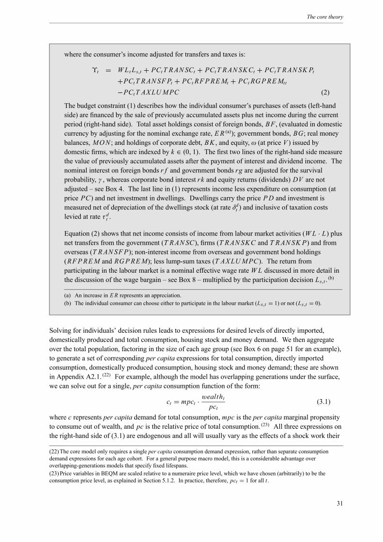
The core theory
where the consumer’s income adjusted for transfers and taxes is:
ϒt = WLt Ls,t + PCtT RANSCt + PCtT RANSKCt + PCtT RANSK Pt+PCtT RANSFPt + PCt RFPREMt + PCt RGPREMtt−PCtT AXLUMPC (2)
The budget constraint (1) describes how the individual consumer’s purchases of assets (left-handside) are financed by the sale of previously accumulated assets plus net income during the currentperiod (right-hand side). Total asset holdings consist of foreign bonds, BF , (evaluated in domesticcurrency by adjusting for the nominal exchange rate, ER (a)); government bonds, BG; real moneybalances, MON ; and holdings of corporate debt, BK , and equity, ω (at price V ) issued bydomestic firms, which are indexed by k ∈ (0, 1). The first two lines of the right-hand side measurethe value of previously accumulated assets after the payment of interest and dividend income. Thenominal interest on foreign bonds r f and government bonds rg are adjusted for the survivalprobability, γ , whereas corporate bond interest rk and equity returns (dividends) DV are notadjusted – see Box 4. The last line in (1) represents income less expenditure on consumption (atprice PC) and net investment in dwellings. Dwellings carry the price PD and investment ismeasured net of depreciation of the dwellings stock (at rate δdt ) and inclusive of taxation costslevied at rate τ dt .
Equation (2) shows that net income consists of income from labour market activities (WL · L) plusnet transfers from the government (T RANSC), firms (T RANSKC and T RANSK P) and fromoverseas (T RANSFP); non-interest income from overseas and government bond holdings(RFPREM and RGPREM); less lump-sum taxes (T AXLUMPC). The return fromparticipating in the labour market is a nominal effective wage rate WL discussed in more detail inthe discussion of the wage bargain – see Box 8 – multiplied by the participation decision Ls,t . (b)
(a) An increase in ER represents an appreciation.(b) The individual consumer can choose either to participate in the labour market (Ls,t = 1) or not (Ls,t = 0).
Solving for individuals’ decision rules leads to expressions for desired levels of directly imported,domestically produced and total consumption, housing stock and money demand. We then aggregateover the total population, factoring in the size of each age group (see Box 6 on page 51 for an example),to generate a set of corresponding per capita expressions for total consumption, directly importedconsumption, domestically produced consumption, housing stock and money demand; these are shownin Appendix A2.1. (22) For example, although the model has overlapping generations under the surface,we can solve out for a single, per capita consumption function of the form:
ct = mpct · wealthtpct(3.1)
where c represents per capita demand for total consumption, mpc is the per capita marginal propensityto consume out of wealth, and pc is the relative price of total consumption. (23) All three expressions onthe right-hand side of (3.1) are endogenous and all will usually vary as the effects of a shock work their
(22)The core model only requires a single per capita consumption demand expression, rather than separate consumptiondemand expressions for each age cohort. For a general purpose macro model, this is a considerable advantage overoverlapping-generations models that specify fixed lifespans.(23)Price variables in BEQM are scaled relative to a numeraire price level, which we have chosen (arbitrarily) to be theconsumption price level, as explained in Section 5.1.2. In practice, therefore, pct = 1 for all t .
31

The Bank of England Quarterly Model
way through the economy. The marginal propensity to consume depends on present and future post-taxinterest rates, present and future consumption prices, habits, and the user cost of housing. Wealthincludes the present value of current and future labour income, the present value of current and futuretaxes and transfers, returns on financial assets, and the current value of housing. The price of the totalconsumption bundle will reflect the effects of domestic demand and supply conditions on the price ofdomestically produced consumption goods, and the effects of shifts in world prices and the exchangerate on the price of imported consumption goods.
The choice of desired housing stock reflects household preferences over durables and non-durables, andthe user cost of housing capital, which depends on depreciation, capital gains, taxes and interest rates.Housing wealth – which is defined in this model as the value of the housing stock brought into thecurrent period – is part of overall wealth that appears in equation (3.1), as housing is a potential store ofvalue from one period to the next. It is tempting to assume from this that housing wealth ‘causes’consumption, as higher house prices would make more wealth available to be used for consumption inthe next period. However, this is not the case under the assumptions of the core theory. Consumers‘gain’ from an increase in house prices because this increases the value of the housing stock broughtforward from the previous period. But consumers also ‘lose’ since it now costs more for households toown houses.
On the other hand, if there had been an exogenous decrease in the housing stock (from, say, anunanticipated ‘depreciation shock’ – a natural disaster, for example) some consumption would need tobe sacrificed over a period of time to rebuild the housing stock. And the housing stock deteriorates eachperiod, so some expenditure will be needed to maintain a constant level of housing stock. (24)
Finally, we include so-called ‘external’ habit formation. Households assess their consumption against adesired level – the reference habit – so that aggregate consumption will be stickier than otherwise. (25) Inother words, households are concerned about the rate of change of their consumption, as well as thelevel over their expected lifetime. This allows us to influence the degree of persistence of consumptionfollowing a shock. Because the habit formation is external, however, the introduction of habits does notnecessarily generate a ‘hump-shaped’ aggregate consumption response to shocks, which is often afeature of models with habit persistence. (26)
3.2.2 Firms
The theory of the firm must provide an account of factor and inventory accumulation, production ofoutput from these factors, the distribution of wealth, and pricing decisions. As with households, we startwith a standard optimisation problem for individual agents, before deriving aggregate decision rules.
Individual firms are assumed to maximise profits given cash-flow constraints and market conditions.They are monopolistically competitive and each sells a single, slightly differentiated good in differentdomestic and foreign markets, while renting labour from households and paying for capital goods.Because firms have some market power, they make a profit on each unit of output such that (abstractingfrom taxes) the value of the firm is greater than the value of its capital stock.
(24)This takes no account of the possible effects on consumption of house price rises, such as through an increase in the abilityto borrow, which we do not attempt to model in the core theory.(25) In the case of ‘external’ habits, the reference habit is typically an aggregate measure of consumption, as opposed toindividual consumption levels, which would be the case of ‘internal’ habits. External habits can be thought of as ‘catching upwith the Joneses’; see Abel (1990). We use the external version of habits to facilitate aggregation in the Blanchard-Yaaristructure.(26)See, for example, Fuhrer (2000).
32
The core theory
In order to provide an account of different expenditures, the goods market is subdivided into privateconsumption, housing investment, capital investment, ‘other’ investment, inventories, governmentprocurement, imports and exports (although firms only produce using a single production function, seeSection 3.3.1). Firms are assumed to sell their production to these different markets, so sales revenuedepends on both sales volumes and prices in these markets. An individual firm aims to sell at a mark-upover its marginal cost and is assumed to face costs of adjusting prices, such that they prefer not tochange prices quickly. At any given time, all firms will choose to adjust their prices by a certain fractiontowards the desired level, depending on current costs, expected inflation, and usually lagged inflation aswell (see also Section 3.4.3). The mark-up is time-varying because of this nominal stickiness, but wouldbe constant if prices adjusted instantly. (27)
A firm’s cash flow is equal to sales revenue less labour costs (the gross wage bill plus employers’ socialsecurity contributions), investment, (net) debt servicing, transfers to overseas residents and domestichouseholds (such as pension contributions), and lump-sum taxes. After paying tax and debt interestpayments, the remainder is distributed to shareholders (households) as dividends.
In order to account for aggregate imports, we build demands for imported consumption goods into theoptimisation problem of the household, and imported capital goods into the optimisation problem for thefirm. We assume that firms desire a particular level of a composite capital good and that capital can besourced from both domestic and overseas production. (28) This implies that the real exchange rate willaffect the user cost of directly imported capital, and hence the supply side. (29) The split betweendomestic and imported capital will depend on their relative prices and on firms’ preferences. (30) Totalcapital is accumulated to match its marginal product (corrected for the mark-up over real marginal costs)with the effective user cost. This is a conventional Jorgensonian function of depreciation, taxes andprice changes. As a default, firms are assumed to face real rigidities in adjusting both the capital stockand investment, which are modelled as quadratic adjustment costs that have no effect on the steady state.These costs are tangible, involving lost output for firms, and therefore affect the marginal returns tocapital when there is dynamic adjustment to equilibrium. (31) The presence of adjustment costs ensuresthat the path to the new steady state is not as jumpy as would be implied by classical investment theory.While there is no explicit variable in the model representing Tobin’s q, the behaviour of investment iscompatible with that theory. (32) However, unlike in the simple textbook representation, the steady-statevalue of Tobin’s q is not unity, because our model assumes monopolistic competition in the goodsmarket and allows for capital taxes.
Total capital is predetermined in the production function, as capital used in the current period must beinstalled in the previous period, but the amount of labour used is decided in each period. Firms bargainwith unions over nominal wages (see Section 3.3.2) and incur adjustment costs in changing employment(just as for capital). We impose a ‘right to manage’ assumption, which means that firms unilaterallydecide on the level of employment, once the wage bargain is complete. This results in an equilibrium inwhich workers are paid their marginal product (adjusted for the mark-up and accounting for adjustmentcosts).
(27) In the steady state, the mark-up on a good is solely a function of the (constant) elasticity of demand in the particularmarket for that good.(28)As we observe from UK trade and National Accounts data.(29)This is different from the basic neoclassical open economy model in which the capital-labour ratio is tied down by theworld real interest rate.(30)Formally, we assume that the capital index is a constant elasticity of substitution (CES) aggregate of imported anddomestically produced capital goods.(31)These losses do not result in payments that benefit any other agent – they are ‘frictions’ that are lost to the macroeconomy.(32)See, for example, Chapter 8 of Romer (1995).
33

The Bank of England Quarterly Model
If capital is predetermined and labour costly to adjust, the marginal cost curve will be steep. Sincepricing decisions are a mark-up over marginal costs, this implies that firms respond to demand shockswith large changes in prices and small changes in production. To create more flexibility for these keymodel properties, we therefore assume that, in the short term, the firm can vary the intensity with whichcapital is used, thereby increasing or decreasing the effective level of capital entering production. (33)
The ability to utilise capital more intensely flattens the short-run marginal cost curve. However, theconsequence of higher (lower) utilisation is higher (lesser) depreciation, as the rate of wear and tear isassumed to increase if machines are run more intensively. In the long run, only an increase in physicalcapital, labour or productivity can generate more output.
With capital and labour in place, firms produce value added using a Constant Elasticity of Substitution(CES) technology. As is well known, an infinite elasticity of substitution means that capital and labourare perfect substitutes, while a zero elasticity of substitution implies a Leontief function, where capitaland labour must be combined in fixed proportions; and an elasticity of one implies a Cobb-Douglastechnology. The motivation for using a CES production function, instead of the simpler Cobb-Douglasform, is that the elasticity of investment to interest rates would be unrealistically high under theassumption of Cobb-Douglas technology. Correspondingly, we assume that capital and labour tend tobe less substitutable for each other than in the Cobb-Douglas case.
Firms also hold inventories. The assumptions we make about expectations, discussed in Section 5.1.5,mean that firms’ decisions on optimal production levels are not affected by uncertainty. As such, thereis no role in the core model for inventories as insurance against demand surprises. Instead, we assumethat firms first make their decisions for capital, labour and prices, and then make a decision about thedesired level of inventories. This target level balances two costs: the expected cost of foregone sales andthe expected opportunity cost of holding stocks. (34) Target inventories will therefore be affected byaverage sales revenue per unit, real marginal costs and real interest rates. Some production is divertedfrom (or added to) sales in order to achieve the desired stock level; the change in stocks enters the goodsmarket clearing condition and is part of total expenditure. As with other factors, we usually assume thatstock adjustment is costly, so that firms are not always at their desired level.
Firms finance their activities by issuing shares and debt. Since we allow firms and consumers todiscount the future at different rates, we impose a debt-equity ratio to prevent firms issuing only debt oronly equity. Shares are valued using the standard dividend discount model, accounting for taxes, whichemerges from the household optimisation problem (see Section 3.3.3 for details).
Each firm is assumed to produce a slightly differentiated good, which gives them market power. Ourmarket structure implies that market power in each goods market is inversely related to the elasticities ofdemand in those markets. (35) As in Blanchard and Kiyotaki (1987), we make the standard assumptionthat there is a large number of such firms and that they behave symmetrically. (36) This allows us toaggregate across firms to get the decision rules for employment, domestically produced and importedcapital, inventory stocks, output, and prices for each domestic market and the export market.
(33)We use the implementation in Burnside and Eichenbaum (1996).(34)The expected cost of lost revenue is proxied by a scalar on next period’s average sales price; given factor costs and interestrates for the storage costs, this dictates the stock-sales ratio. This is a version of the model in Kahn (1987).(35)This is a very useful simplification, for example, see Dixit and Stiglitz (1977).(36)That is, firms are assumed to make the same pricing and factor decisions. See pages 235-236 of Walsh (2003) for details.
34
The core theory
We assume that prices are sticky because firms want to avoid changing prices. We do this by assumingprice adjustment costs in firms’ ‘disutility’, as in Rotemberg (1982), (37) which means that aggregation issimple and direct. Price adjustment costs are intangible in the sense that firms do not incur direct costs,like labour and capital adjustment costs in our model or in ‘menu cost’ approaches such as Mankiw(1985). (38) An alternative pricing assumption would have been that of Calvo (1983), which we use inthe union wage bargaining context (see Section 3.3.2). In a Calvo setting, only a (randomly selected)proportion of firms would be allowed to change their price at a given date. The aggregate price levelwould therefore be a weighted average of newly set prices and prices set in the past. These differentprices would create a source of heterogeneity among firms, implying that firms would chose differentlevels of employment, capital stocks and utilisation rates. In addition, we would have to account for thefact that firms have different labour demand schedules in our wage bargaining framework – so thataggregation problems would ‘spill over’ into other markets. (39) For tractability, therefore, we assumeRotemberg price adjustment costs, which means that firms behave identically in changing their prices,unlike in the Calvo setting or if fixed-term pricing contracts were assumed. (40) This means that we cantalk about ‘the firm’, even though a continuum of differentiated firms underlies the decision rules.
3.2.3 The government
The main requirement for the government sector is to be able to account for fiscal revenues andexpenditures, at a level that is detailed enough to be able to model the effects of government policydecisions on the demands for goods and labour. (41) This flow accounting needs to be matched by stockaccounting that draws out the implications for the supply of government debt to financial markets.
Importantly, we do not need to use the model to analyse public finance issues, and so we are able toabstract from an analysis of optimal fiscal decisions arising from social preferences. This simplifiedpurpose means that we can assume a fairly simple fiscal reaction function, given policy targets; we donot need to distinguish between central and local government; and the government redistributesresources according to some simple rules. The government gains revenue from taxes, issuing debt andseigniorage, while making expenditures on government purchases of goods and labour, transfers, anddebt servicing. As with households, debt is not allowed to follow an explosive path. This solvencycondition is ensured by enforcing the period-by-period fiscal budget constraint, along with a fiscalreaction function. We assume that the government has targets for debt, spending (on goods and onlabour) and transfers, so that it does not generally follow a balanced budget each period. Moreover, debtand spending are allowed to vary temporarily from their target levels following a shock.
(37)See Pesenti (2002) for an example of another recent model that uses the Rotemberg pricing model.(38)Allowing price adjustment to result in direct costs would not have a first-order effect on pricing decisions. However, itwould require us to allocate these adjustment costs to an element of the National Accounts data.(39) It becomes difficult to aggregate individual decisions across the population of firms without additional simplifications(such as an economy-wide rental market for capital goods). While considerable progress has been made in this respect (see forexample Chapter 5 of Woodford (2003)), the aggregation usually relies on log-linearisation of decision rules around aparticular steady state. This is not suitable for our purposes, because we retain the decision rules in levels in order to analyseshocks that change the steady state of the model. In any case, the resulting pricing behaviour is likely to be similar to adoptingthe Calvo approach: in simple models, the two approaches yield identical (to a first-order approximation) reduced-form pricingequations, as shown by Rotemberg and Woodford (1999) for example.(40)Neither the Rotemberg nor Calvo alternatives are necessarily realistic descriptions of pricing behaviour at the level ofindividual firms. At that level, it seems more likely that frictions such as menu costs are perhaps more relevant. Whenchoosing a specification for nominal rigidities in a general purpose macroeconomic model, however, tractability is often thedeciding factor.(41)Box 3 on page 36 discusses the relationship between private sector and government output.
35
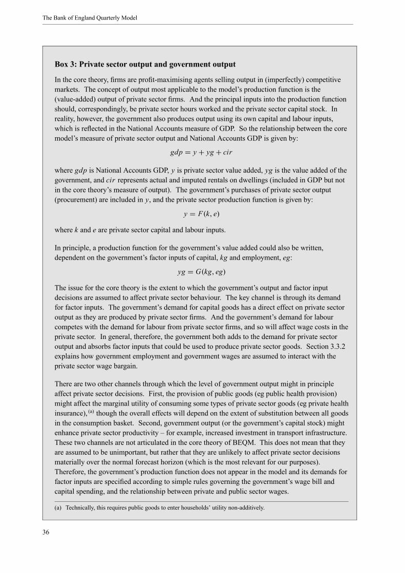
The Bank of England Quarterly Model
Box 3: Private sector output and government output
In the core theory, firms are profit-maximising agents selling output in (imperfectly) competitivemarkets. The concept of output most applicable to the model’s production function is the(value-added) output of private sector firms. And the principal inputs into the production functionshould, correspondingly, be private sector hours worked and the private sector capital stock. Inreality, however, the government also produces output using its own capital and labour inputs,which is reflected in the National Accounts measure of GDP. So the relationship between the coremodel’s measure of private sector output and National Accounts GDP is given by:
gdp = y + yg + cir
where gdp is National Accounts GDP, y is private sector value added, yg is the value added of thegovernment, and cir represents actual and imputed rentals on dwellings (included in GDP but notin the core theory’s measure of output). The government’s purchases of private sector output(procurement) are included in y, and the private sector production function is given by:
y = F(k, e)where k and e are private sector capital and labour inputs.
In principle, a production function for the government’s value added could also be written,dependent on the government’s factor inputs of capital, kg and employment, eg:
yg = G(kg, eg)The issue for the core theory is the extent to which the government’s output and factor inputdecisions are assumed to affect private sector behaviour. The key channel is through its demandfor factor inputs. The government’s demand for capital goods has a direct effect on private sectoroutput as they are produced by private sector firms. And the government’s demand for labourcompetes with the demand for labour from private sector firms, and so will affect wage costs in theprivate sector. In general, therefore, the government both adds to the demand for private sectoroutput and absorbs factor inputs that could be used to produce private sector goods. Section 3.3.2explains how government employment and government wages are assumed to interact with theprivate sector wage bargain.
There are two other channels through which the level of government output might in principleaffect private sector decisions. First, the provision of public goods (eg public health provision)might affect the marginal utility of consuming some types of private sector goods (eg private healthinsurance), (a) though the overall effects will depend on the extent of substitution between all goodsin the consumption basket. Second, government output (or the government’s capital stock) mightenhance private sector productivity – for example, increased investment in transport infrastructure.These two channels are not articulated in the core theory of BEQM. This does not mean that theyare assumed to be unimportant, but rather that they are unlikely to affect private sector decisionsmaterially over the normal forecast horizon (which is the most relevant for our purposes).Therefore, the government’s production function does not appear in the model and its demands forfactor inputs are specified according to simple rules governing the government’s wage bill andcapital spending, and the relationship between private and public sector wages.
(a) Technically, this requires public goods to enter households’ utility non-additively.
36
The core theory
For simplicity, government bonds take the form of single-period nominal bonds. Governmentemployment and purchases are assumed not to add to the productive capital stock or contribute tohousehold utility. (42) Transfers are made to households, firms and the rest of the world, based on targetratios to output. There is a wide range of taxes: on households and firms, directly on income andexpenditure, on stocks and flows, and distortionary and lump-sum. In practice, some of these will be setto zero, if we cannot split them out when looking at the aggregate tax data. But they are included toallow a wide range of scenarios to be considered.
The fiscal side of the model is closed by specifying an element of the budget constraint to be theendogenous instrument. Virtually any item in the government budget constraint could be used as thefiscal instrument (in principle, more than one element could be chosen), as long as the constraint is notviolated. The fiscal reaction function specifies that the government varies tax revenue according to thedifference between debt and its target and the rate of change of the outstanding debt stock. This impliesthat debt initially acts as a buffer following a shock, before settling back to its long-run target level. (43)
As a default, a single household tax is normally assumed to be the endogenous instrument, with targetratios for the remaining taxes relative to the relevant flows.
3.2.4 The monetary authority
The monetary authority anchors the nominal side of the economy. As with fiscal policy, we assume asimple reaction function for the monetary authority, rather than an optimising strategy. A number ofdifferent targets, instruments and reaction functions could be specified. The current default that ensuresthat the nominal side is anchored in the long run is a simple Taylor rule in which the short-term(one-period) nominal interest rate is used to ensure that annual CPI inflation is ultimately maintained at atarget level of 2%. Some smoothing of the nominal interest rate is usually assumed. (44)
3.2.5 The external sector
The characterisation of overseas agents is the most simplified of all. Consistent with the specification ofa small open economy, the actions of overseas agents are characterised by exogenous paths for the worldinterest rate, world prices and inflation, and overseas demand. The domestic economy is completelysmall in capital markets, which means that there are no restrictions on the flow of foreign capital anddomestic agents are price-takers in foreign capital markets. Monetary and fiscal policy actions in thedomestic economy do not, therefore, affect interest rates in the rest of the world. The domestic economyis not completely small in international goods markets: domestic and foreign goods are differentiatedand have different (common currency) prices. Foreign demand for domestic goods depends on therelative (common currency) price of domestic and foreign goods. (45)
One of the key features of this model is that it determines an equilibrium real exchange rate. (46) There isno simple reduced-form expression for the real exchange rate, but the equilibrium real exchange rate can
(42)Since these goods do not enter the household utility or private sector production functions, and government policy followssimple rules, it is not necessary to specify a production function for public goods.(43)This is how the model is set to work when simulating the response to shocks. Given the purpose of the government sectorin BEQM, we use a simple reaction function rather than attempting to model optimal fiscal strategy. When used for forecasts,assumptions from HM Treasury about fiscal variables are conventionally imposed over the forecast horizon.(44)For forecasts, constant or market interest rates are imposed over the forecast horizon. See Chapter 5 for a fuller discussion.(45) If the domestic economy were completely small, domestic exports and foreign goods would sell at a common price, andforeign demand for domestic exports would be perfectly elastic.(46)The real exchange rate is defined as the nominal exchange rate adjusted for the relative consumer price levels between thedomestic economy and the rest of the world. This definition is different from the definition of the real exchange rate as theratio of tradable and non-tradable goods prices that is common in recent work in ‘new open economy’ models.
37

The Bank of England Quarterly Model
be thought of as the relative price that ensures that export demand clears the domestically producedgoods market and maintains internal balance (see Section 3.3.1). Additionally, the current accountequilibrium is the flow equilibrium consistent with the net foreign asset stock equilibrium; the realexchange rate is the relative price consistent with this flow. In the steady state, these all settle to constantlevels (abstracting from growth). Hence household choice, firms’ decisions, and domestic policy allcontribute to determining the value of the real exchange rate, given conditions in the rest of the world.
The current and capital account identities are not explicit in the model but are standard and enforced.The capital account is simply the change in the net foreign asset position, and is equal in magnitude andopposite in sign to the current account. The current account is the sum of net trade, foreign asset returns(which reflect interest payments and real exchange rate changes) and net transfers between domestic andoverseas agents. Net foreign asset accumulation can therefore be defined as output less domesticexpenditure, foreign debt servicing and net transfers, so that the net foreign asset stock reflects the gapbetween domestic supply and demand flows.
3.3 Characterisation of the markets
Having described the motivations of agents, we now set out the characteristics of the markets in whichthey interact: goods markets, a domestic labour market and financial markets.
3.3.1 Goods markets
The characterisation of goods markets has to be sufficient to describe equilibrium in demand and supply,which is a statement about how production is cleared. At the same time, we have to be able to mapmodel concepts to National Accounts data. We assume that private sector firms add value using capitaland labour. The measure this corresponds to is private sector value added. (47) This approach raisesthree key issues. First, the choice of a single production function on the supply side makes it difficult tosay anything about different expenditure deflators. Second, a significant proportion of imported goodsare intermediates in production, so we need some extra modelling to account for final private sectoroutput. Finally, we need to match private sector inputs with private sector output. We describe belowhow we have attempted to tackle these issues – in particular, how we have dealt with the inherent tensionbetween using a single production function and the need to differentiate between expenditures.
Consider first production from firms. As we saw in Section 3.2.2, we assume a continuum of firms andthat each produces a slightly differentiated output. Product differentiation is the source of market powerand the foundation for thinking about sticky prices. We aggregate the decision rules of firms, so thatwhen we talk about output produced by ‘the’ firm, we are referring to a composite index of production.
We take this index to be a measure of value-added production. Firms produce finished goods fromcapital and labour: F (k, e) ≡ y. (48) To reconcile different categories of expenditure with goods from asingle production function, we assume that firms can distribute production to different markets foralternative uses – so the composite good is a sort of wondrous substance that is used for domesticnon-durable consumption, accumulation of durables (housing), domestic capital expenditure,stockbuilding, government spending on private sector output, and exports.
(47)To avoid potential distortions to real output measures arising from differing indirect tax rates across expenditurecomponents, we use real value added at basic prices.(48) In practice, output is defined net of capital and adjustment costs (see equation (A.30) in Appendix A)
38
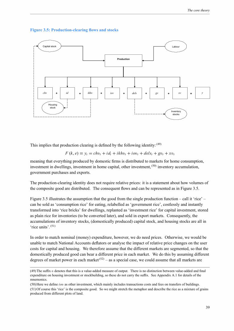
The core theory
Figure 3.5: Production-clearing flows and stocks
chv id iov + gv xv = y
Capital stock Labour
Production
+ +
Housing stock
+ dels
Inventory stocks
+ + ikhv
This implies that production clearing is defined by the following identity: (49)
F (k, e) ≡ yt = chvt + idt + ikhvt + iovt + delst + gvt + xvtmeaning that everything produced by domestic firms is distributed to markets for home consumption,investment in dwellings, investment in home capital, other investment, (50) inventory accumulation,government purchases and exports.
The production-clearing identity does not require relative prices: it is a statement about how volumes ofthe composite good are distributed. The consequent flows and can be represented as in Figure 3.5.
Figure 3.5 illustrates the assumption that the good from the single production function – call it ‘rice’ –can be sold as ‘consumption rice’ for eating, relabelled as ‘government rice’, costlessly and instantlytransformed into ‘rice bricks’ for dwellings, replanted as ‘investment rice’ for capital investment, storedas plain rice for inventories (to be converted later), and sold in export markets. Consequently, theaccumulations of inventory stocks, (domestically produced) capital stock, and housing stocks are all in‘rice units’. (51)
In order to match nominal (money) expenditure, however, we do need prices. Otherwise, we would beunable to match National Accounts deflators or analyse the impact of relative price changes on the usercosts for capital and housing. We therefore assume that the different markets are segmented, so that thedomestically produced good can bear a different price in each market. We do this by assuming differentdegrees of market power in each market (52) – as a special case, we could assume that all markets are
(49)The suffix v denotes that this is a value-added measure of output. There is no distinction between value-added and finalexpenditure on housing investment or stockbuilding, so these do not carry the suffix. See Appendix A.1 for details of themnemonics.(50)Here we define iov as other investment, which mainly includes transactions costs and fees on transfers of buildings.(51)Of course this ‘rice’ is the composite good. So we might stretch the metaphor and describe the rice as a mixture of grainsproduced from different plots of land.
39

The Bank of England Quarterly Model
equally competitive, so that all goods are effectively sold in one market. Clearly, this is a compromisebecause we are trying to account for differences in the price elasticities of demand for different goods.This ignores technological factors, but a more fully articulated multisectoral setting would be needed toaccount for them properly. (53)
The analogue to the production clearing condition depicted in Figure 3.5 is a goods market clearingcondition that accounts for imported goods – both final and intermediate goods. The total demand forimports is not modelled by a single equation, but comes from the demands for imported finalconsumption and final capital goods from the maximisation problems for households and firms (as wellas intermediate imports, see below). (54) However, we cannot just add imported goods to the picture inFigure 3.5, as we are then adding ‘corn’ to ‘rice’. We can, however, reconcile expenditure on domesticand imported goods by an identity that divides total money expenditure into consumption, investment,stock-building, government procurement, exports and imports.
We also need to account for imports of intermediate goods, which form a significant proportion of totalimports and enter the production process creating the final output that is divided between expenditurecategories. Clearly, one way of dealing with intermediate imports would be to model a two-stageproduction process, where intermediates were potentially inputs into domestic production and a factor offinal production itself, but this would require a more fully structured multisectoral setting. Alternatively,we could model output as a function of capital, labour and imported intermediates, but this would meanhaving to subtract a proportion from output in order to match real production clearing on a value-addedbasis. We assume instead that intermediates must be combined with domestically produced goods infixed proportions, which vary according to expenditure category. (55) This allows us to match NationalAccounts concepts while ensuring that consistent market clearing conditions hold. It has the addedadvantage that the demand for intermediates depends on the composition of expenditure, which is also afeature of the data.
The focus on private sector firms means that we have to take account of the effects of government valueadded and government employment. This is chiefly a matter of ensuring that data series are definedappropriately, as described in Box 3 on page 36.
3.3.2 The labour market and unions
Labour market interactions have implications for household income (hence financial asset accumulationand the current account), capital investment (hence wealth generation), net government revenues(through labour tax revenues and government expenditure on wages and benefits, hence deficits andgovernment debt), and nominal wages (hence firms’ costs and inflation). The labour market has to beable to provide an account of non-competitive labour market outcomes – to match observed labourmarket behaviour – and also movements in labour market participation, employment andunemployment.
(52)We use a form of monopolistic competition that ensures that elasticities of demand and market power are inversely relatedand controlled by the same parameter – see Blanchard and Kiyotaki (1987). In general, we would expect market entry and exitto affect mark-ups in monopolistic competition, but that would make aggregation substantially more complicated and would beimpractical for a general purpose model such as this.(53)Pesenti (2002) illustrates a multisectoral treatment of relative prices in an open economy.(54)We could include imported goods in government expenditure, but these are not significant in the data.(55)This is as if we have introduced another layer of firms into the model, which sell gross home consumption and capitalgoods to domestic households and firms by combining imported intermediate goods with value-added goods using a Leontieftechnology. Unlike the firms in Section 3.2.2, they do not use capital or labour. If we assume that these firms are perfectlycompetitive, they will make no profit themselves and hence contribute nothing to value added.
40

The core theory
In some models, non-competitive wage outcomes are generated by assuming that workers have a degreeof market power, because they each offer a differentiated labour service. (56) However, in such modelsthe choice variable of both households and firms is hours worked, so the labour market always clears.This means that everyone is employed, and hours worked and the real wage move to clear the labourmarket. (57) Formally, this is because labour market equilibrium implies a real wage that clears demandand supply for labour (in hours). We therefore need to introduce an additional relationship – a‘wage-setting’ curve – that will allow us to model unemployment.
We could use several devices: matching models (see, for example, Mortensen and Pissarides (1994)),insider-outside models (see Layard, Nickell and Jackman (1991) and references therein) or unionbargaining models (see Manning (1993)). We have retained the same kind of bargaining framework thatwas used in the MTMM model. This should be thought of as a metaphor to generate the outcomes wewant, rather than a literal description of the UK labour market. The implementation here is structuraland so needs to take account of general equilibrium issues that are not usually dealt with in othersettings.
Labour supply is determined by a binary choice made about participation: workers decide to enter thelabour market if the expected return from doing so exceeds their ‘reservation’ (participation) wage – thedecision here is whether or not to enter the labour market, not about how much labour to supply. Theexpected return from entering the labour market is a weighted average of private sector (post-tax) wages,public sector (post-tax) wages and unemployment benefits. (58) The reservation wage reflects themarginal disutility of work, relative to not working, which we assume is exogenously distributed acrosshouseholds. The level of employment is chosen by firms to maximise profits.
Unions bargain on workers’ behalf. In any given period, a proportion of (randomly chosen) unionsengage with firms in a bargain over the nominal wages of the workers they represent. This fraction isconstant, so that we have Calvo (1983) nominal wage setting, rather than contracts for fixed terms as inTaylor (1980). (59) Unions aim to maximise the welfare of an average worker, so the value of the‘outside’ earnings that could be received if employed by the government or unemployed has a role toplay. The private sector wage is determined as the Nash equilibrium in which the firms’ and unions’strategies are both optimal. The wages of government employees are set according to a simple rulelinking government and private sector wages. (60)
The natural rate of unemployment in this model depends on many factors, including those affecting thewage bargain: the reservation wage, technology, goods and labour market conditions, taxation andbenefits, and unions’ preferences and power. The real exchange rate can affect the natural rate boththrough profitability and through labour supply decisions (because workers care about their wage interms of their ability to purchase a bundle of consumption goods).
The interaction of the factors described above in the labour market defines an outcome for numbersemployed. For simplicity, we assume that average hours worked are given exogenously.
(56) In those models, workers seek a mark-up of their wages over their own implicit costs of working (such as the opportunitycost of leisure), just as firms seek a mark-up over real marginal costs. See, for example, Erceg, Henderson and Levin (2000).(57)Galí (1996) employs a mapping from hours directly into unemployment in order to get, partially, around this problem.(58)The weights reflect the probabilities of being employed in the private sector or public sector or of being unemployed. SeeBox 8 on page 58.(59)While contracts for fixed terms may be more realistic, Calvo-style contracts are particularly tractable. Our assumptionhere contrasts with the discussion of firms’ pricing in Section 3.2.2. We find Calvo pricing assumption more tractable for thelabour market than for firms.(60)Box 3 on page 36 discusses the relationship between private sector and government output.
41
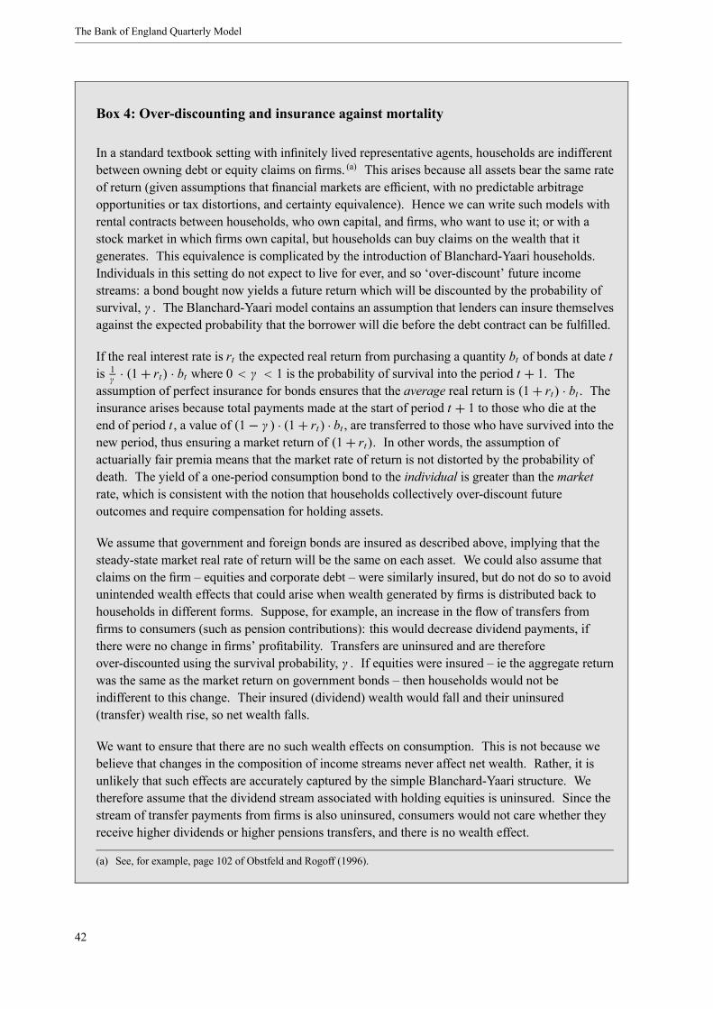
The Bank of England Quarterly Model
Box 4: Over-discounting and insurance against mortality
In a standard textbook setting with infinitely lived representative agents, households are indifferentbetween owning debt or equity claims on firms. (a) This arises because all assets bear the same rateof return (given assumptions that financial markets are efficient, with no predictable arbitrageopportunities or tax distortions, and certainty equivalence). Hence we can write such models withrental contracts between households, who own capital, and firms, who want to use it; or with astock market in which firms own capital, but households can buy claims on the wealth that itgenerates. This equivalence is complicated by the introduction of Blanchard-Yaari households.Individuals in this setting do not expect to live for ever, and so ‘over-discount’ future incomestreams: a bond bought now yields a future return which will be discounted by the probability ofsurvival, γ . The Blanchard-Yaari model contains an assumption that lenders can insure themselvesagainst the expected probability that the borrower will die before the debt contract can be fulfilled.
If the real interest rate is rt the expected real return from purchasing a quantity bt of bonds at date tis 1γ· (1+ rt) · bt where 0 < γ < 1 is the probability of survival into the period t + 1. The
assumption of perfect insurance for bonds ensures that the average real return is (1+ rt) · bt . Theinsurance arises because total payments made at the start of period t + 1 to those who die at theend of period t , a value of (1− γ ) · (1+ rt) · bt , are transferred to those who have survived into thenew period, thus ensuring a market return of (1+ rt). In other words, the assumption ofactuarially fair premia means that the market rate of return is not distorted by the probability ofdeath. The yield of a one-period consumption bond to the individual is greater than the marketrate, which is consistent with the notion that households collectively over-discount futureoutcomes and require compensation for holding assets.
We assume that government and foreign bonds are insured as described above, implying that thesteady-state market real rate of return will be the same on each asset. We could also assume thatclaims on the firm – equities and corporate debt – were similarly insured, but do not do so to avoidunintended wealth effects that could arise when wealth generated by firms is distributed back tohouseholds in different forms. Suppose, for example, an increase in the flow of transfers fromfirms to consumers (such as pension contributions): this would decrease dividend payments, ifthere were no change in firms’ profitability. Transfers are uninsured and are thereforeover-discounted using the survival probability, γ . If equities were insured – ie the aggregate returnwas the same as the market return on government bonds – then households would not beindifferent to this change. Their insured (dividend) wealth would fall and their uninsured(transfer) wealth rise, so net wealth falls.
We want to ensure that there are no such wealth effects on consumption. This is not because webelieve that changes in the composition of income streams never affect net wealth. Rather, it isunlikely that such effects are accurately captured by the simple Blanchard-Yaari structure. Wetherefore assume that the dividend stream associated with holding equities is uninsured. Since thestream of transfer payments from firms is also uninsured, consumers would not care whether theyreceive higher dividends or higher pensions transfers, and there is no wealth effect.
(a) See, for example, page 102 of Obstfeld and Rogoff (1996).
42
The core theory
We have found that this effect is potentially non-trivial: gross income flows have been constructedto match the National Accounts and can change substantially. Our assumptions ensure that thesetransfers net out in terms of private sector income flows, but they would not net out in terms ofprivate sector wealth if we assumed that equities were insured. If equities were uninsured andcorporate debt insured, the average rate of return on the household financial asset portfolio woulddepend on the composition of bonds and equities, and firms would not be indifferent to the sourceof their finance. We want to avoid this too, so we assume that corporate debt is uninsured. We alsoassume that firms and consumers discount the future at different rates, which allows leverage overthe cost of capital without having to change the household over-discounting parameter, γ . Withinthis structure, an exogenous debt-equity ratio determines the level of outstanding corporate debt.
3.3.3 Financial and asset markets
Financial prices equate the demand and supply of financial assets, which in turn reflect underlyingequilibrium in the goods and labour markets. As we saw in Figure 3.2, an important relation in themodel is that households’ aggregate demand for financial assets is met by the domestic supply of assets(equities, corporate debt and government debt) and overseas supply of (net) assets. A steady-stateposition is reached when equilibrium flows are at levels that sustain unchanging (adjusted for growth)asset stock positions at their desired levels. For example, the net foreign asset position is stable whenthe current account generates exactly enough net income to finance the net interest payments on netforeign assets. To reach a steady-state position, flows must adjust over time so that the assets can beaccumulated (or decumulated) to the desired long-run level. For example, a rise in desired net foreignassets requires, on average, smaller current account deficits (or larger surpluses) during the transitionperiod.
A key simplification of the treatment of asset prices arises from assuming certainty equivalence (seeChapter 5). In practice, this means that a single risk-free market rate of return is used to value assets.
A further simplification is that we have not attempted to model a layer of financial intermediation.Instead, we assume that households own claims on firms, government and overseas residents. Themodel is not, therefore, directly useful for issues where financial intermediation is of first-orderimportance, such as collateral effects and financial accelerator phenomena. (61) We prefer to look at suchissues using separate, more specialised models and keep the balance sheet dimension of the macromodel as simple as possible.
The most basic asset in the model is a one-period nominal bond. These bonds can be issued by firms, bythe government or by households. Technically, we only allow households to trade bonds with overseasresidents, but the net effect is equivalent to allowing firms to hold gross investment positions in foreignassets and liabilities. As the economy is completely small and open in capital markets, uncoveredinterest parity (UIP) is a standard no-arbitrage condition that prices the exchange rate to equalise thereturn on riskless domestic and foreign bonds. Firms can issue shares, which are priced according to thestandard (post-tax) dividend discount model. (62)
(61)See, inter alia, Bernanke, Gertler and Gilchrist (1999).(62)A complication in the Blanchard-Yaari setting is that individuals ‘over-discount’ because they do not expect to live forever, so it is assumed that households can insure themselves. But this means that certain additional assumptions (set out in Box4 on page 42) are required to prevent undesirable wealth effects.
43

The Bank of England Quarterly Model
The difference between the supply of domestic financial assets and households’ demand for financialassets is taken up fully by overseas residents in the form of net foreign assets. (63) These aresingle-period bonds priced in foreign currency units, so exchange rate changes will affect the value ofdomestic households’ portfolios. Although the level of total financial assets held does reflect anoptimisation decision by households, there is no portfolio choice because there is no risk-return trade-offto balance across different assets.
Asset stocks and prices can reveal potentially important information. Figure 3.2 shows how agents arelinked by asset markets. Household financial assets are composed of liabilities from government, firms,and overseas residents. The value of firms’ liabilities reflects decisions about pricing, wage payments,employment, capital, utilisation rates and inventory accumulation. The value of government liabilitieswill reflect policy decisions for taxes, transfers and spending, given demand conditions. Finally, thevalue of foreign assets will reflect movements in the current account and the exchange rate.
3.4 The nominal side of the economy and monetary transmission
The previous discussion focused on the real side of the model economy. But the analysis of inflationrequires attention to nominal magnitudes and to the determinants of nominal wages and prices.
3.4.1 Money market equilibrium
Money in BEQM is modelled as a non-interest bearing government liability that enters the governmentbudget constraint through seigniorage. We create a demand for money by the introduction of realmoney balances to the utility function of households, but money has no idiosyncratic features over andabove those of any other good. (64) So money is dominated by assets earning a positive nominal rate ofreturn, and households would not choose to hold any of their portfolio in money if it were not includedin the utility function. (65)
Given households’ demand for money, the actions of the monetary authority determine the moneysupply. This can be targeted directly or can react to the effects of interest rate changes, as discussed inSection 3.4.4, depending on the assumed monetary policy reaction function. With an inflation targetpursued through interest rates, the assumptions about a balanced real growth equilibrium imply that themoney stock grows at the same rate as nominal output in the steady state.
Without nominal rigidities, the market equilibrium outcomes for real variables and relative prices wouldbe independent of the supply of money, and the model could be thought of as an exchange economy withno role for money or nominal prices. In such a case, equilibrium in the money market would determinethe price level to satisfy households’ demand for real money balances.
However, when there are nominal rigidities as in BEQM, the determination of nominal prices and realvariables cannot be separated in this way. Relative prices are slower to adjust and changes in nominaland real variables are jointly determined, because demand and supply decisions are affected by therelative prices of goods and factors of production. So nominal prices and inflation will depend on thebehaviour of households, firms, the rest of the world and the monetary authority.
(63)The theoretical structure determines net positions, but does not say anything about gross positions.(64)As discussed in Chapter 2 of Walsh (2003), there are a variety of assumptions that can be used to introduce a role formoney in general equilibrium models. We choose the money in utility approach for tractability.(65)Chapter 2 of Woodford (2003) presents analysis of a ‘cashless economy’. This analysis shows that monetary equilibriumcan be sustained in a model in which the traditional motivations for money demand (transactions costs, cash in advanceconstraints) are absent.
44

The core theory
While monetary policy can have short-run effects on the real economy, BEQM is, by construction,neutral with respect to the price level in the long run. (66) But the presence of Blanchard-Yaarihouseholds means that the model is potentially non-superneutral (that is, the equilibrium level of outputwill be affected by the inflation rate). (67) The size of such effects depends on the parameters of themodel, but they are quantitatively small under the current parameterisation.
3.4.2 Nominal wages and prices
As noted in Sections 3.2.2 and 3.3.1, firms operate in imperfectly competitive markets and are thereforeable to sell goods at a mark-up on costs, which we assume can differ across markets. This will bereflected in different relative prices in the long run.
As described in Section 3.3.1, imports are made up of final consumption and capital goods, andintermediate goods for consumption, capital investment, government purchases and exports. We assumelocal currency pricing, which implies gradual pass-through of foreign price shocks to domestic prices(when prices are sticky). The model assumes long-run relative purchasing power parity, as a feature ofthe balanced-growth equilibrium.
Export prices are set in foreign currency and are subject to the same form of price adjustment costs asdomestic prices. This ‘pricing to market’ behaviour provides a short-term channel through which theexchange rate affects export prices in terms of domestic currency.
The inclusion of intermediate goods implies an extra channel for price effects. Given the assumptions offixed shares of gross domestic goods and intermediate imports, the relative price of, say, final homeconsumption is a weighted average of the price of home consumption value added and the price of(imported) intermediate goods. So shifts in imported intermediate costs will (eventually) be passed onin full to consumers. Imported intermediate goods are also used in the production of exports, sodomestic export prices will depend on foreign prices through two channels: the competition effectdescribed above, and the effect of intermediate import costs.
In addition, the production process for each type of good is assumed to be subject to indirect taxes,which are assumed to be passed on fully into final prices. The final price of each good in NationalAccounts terms is a market price – that is, inclusive of indirect taxes – as opposed to a basic price. Eachexpenditure category has a different weight of indirect taxes in final prices. Section 3.3.1 describes howvalue-added output is combined with imported intermediates in fixed proportions, and we employ thesame assumption for indirect taxes. (68) A rise in indirect tax rates leads to a change in final pricesrelative to basic prices. (69)
(66)That is, the economy’s real equilibrium is not affected by the general price level.(67)See Orphanides and Solow (1990). The steady-state inflation rate changes the real value of seigniorage in the governmentbudget constraint. As discussed in Section 3.2.1, the Blanchard-Yaari structure is non-Ricardian and so a change in the real taxburden can have effects on net wealth and consumption.(68)As discussed in Chapter 6, the final price is therefore a weighted average of three components: the price of domestic valueadded; the price of imported intermediates; and indirect taxes.(69)Market prices include indirect taxes (net of subsidies) on both products and production in the National Accounts. Basicprices only include taxes on production. Taxes on products are defined as taxes linked to the sale of a unit of output, such asVAT and duties on fuel and tobacco, and are typically passed on directly in prices paid by consumers. Taxes on production, onthe other hand, are taxes on the overall process and are typically based on the use of fixed capital or the right to undertakeparticular activities; examples include local authority business rates and vehicle excise duty levied on firms.
45
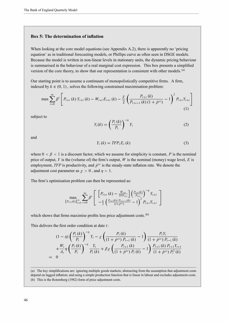
The Bank of England Quarterly Model
Box 5: The determination of inflation
When looking at the core model equations (see Appendix A.2), there is apparently no ‘pricingequation’ as in traditional forecasting models, or Phillips curve as often seen in DSGE models.Because the model is written in non-linear levels in stationary units, the dynamic pricing behaviouris summarised in the behaviour of a real marginal cost expression. This box presents a simplifiedversion of the core theory, to show that our representation is consistent with other models. (a)
Our starting point is to assume a continuum of monopolistically competitive firms. A firm,indexed by k ∈ (0, 1) , solves the following constrained maximisation problem:
max∞
i=0β i Pt+i (k) Yt+i (k)−Wt+i Et+i (k)− χ2
Pt+i (k)Pt+i−1 (k) (1+ pss) − 1
2
Pt+i Yt+i
(1)
subject to
Yt(k) = Pt (k)Pt
−ηYt (2)
andYt (k) = TFPt Et (k) (3)
where 0 < β < 1 is a discount factor, which we assume for simplicity is constant, P is the nominalprice of output, Y is the (volume of) the firm’s output, W is the nominal (money) wage level, E isemployment, TFP is productivity, and pss is the steady-state inflation rate. We denote theadjustment cost parameter as χ > 0 , and η > 1.
The firm’s optimisation problem can then be represented as:
max{Pt+i (k)}∞i=0∞
i=0β i
⎡⎣ Pt+i (k)− Wt+iTFPt+i
Pt+i (k)Pt+i
−ηYt+i
−χ2
Pt+i (k)/Pt+i−1(k)(1+ pss) − 1 2
Pt+iYt+i
⎤⎦which shows that firms maximise profits less price adjustment costs. (b)
This delivers the first order condition at date t :
(1− η) Pt (k)Pt
−ηYt − χ Pt (k)
(1+ pss) Pt−1 (k) − 1PtYt
(1+ pss) Pt−1 (k)+WtAtη
Pt (k)Pt
−η YtPt (k)
+ βχ Pt+1 (k)(1+ pss) Pt (k) − 1
Pt+1 (k) Pt+1Yt+1(1+ pss) P2t (k)
= 0
(a) The key simplifications are: ignoring multiple goods markets; abstracting from the assumption that adjustment costsdepend on lagged inflation; and using a simple production function that is linear in labour and excludes adjustment costs.(b) This is the Rotemberg (1982) form of price adjustment costs.
46
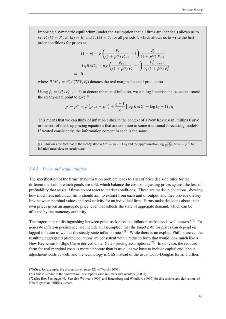
The core theory
Imposing a symmetric equilibrium (under the assumption that all firms are identical) allows us toset Pt (k) = Pt , Et (k) = Et and Yt (k) = Yt for all periods t , which allows us to write the firstorder conditions for prices as:
(1− η)− χ Pt(1+ pss) Pt−1 − 1
Pt(1+ pss) Pt−1
+ηRMCt + βχ Pt+1(1+ pss) Pt − 1
P2t+1Yt+1Yt (1+ pss) P2t
= 0
where RMCt ≡ Wt/ (TFPt Pt) denotes the real marginal cost of production.
Using pt ≡ (Pt/Pt−1 − 1) to denote the rate of inflation, we can log-linearise the equation aroundthe steady-state point to give: (a)
pt − pss = β pt+1 − pss + η − 1χ
log RMCt − log (η − 1) /η
This means that we can think of inflation either in the context of a New Keynesian Phillips Curveor the sort of mark-up pricing equations that are common in some traditional forecasting models.If treated consistently, the information content in each is the same.
(a) This uses the fact that in the steady state RMC = (η − 1) /η and the approximation log 1+ pt1+ pss ≈ pt − pss forinflation rates close to steady state.
3.4.3 Price and wage inflation
The specification of the firms’ maximisation problem leads to a set of price decision rules for thedifferent markets in which goods are sold, which balance the costs of adjusting prices against the loss ofprofitability that arises if firms do not react to market conditions. These are mark-up equations, showinghow much rent individual firms should aim to extract from each unit of output, and they provide the keylink between nominal values and real activity for an individual firm. Firms make decisions about theirown prices given an aggregate price level that reflects the state of aggregate demand, which can beaffected by the monetary authority.
The importance of distinguishing between price stickiness and inflation stickiness is well known. (70) Togenerate inflation persistence, we include an assumption that the target path for prices can depend onlagged inflation as well as the steady-state inflation rate. (71) While there is no explicit Phillips curve, theresulting aggregated pricing equations are consistent with a reduced form that would look much like aNew Keynesian Phillips Curve derived under Calvo pricing assumptions. (72) In our case, the reducedform for real marginal costs is more elaborate than is usual, as we have to include capital and labouradjustment costs as well, and the technology is CES instead of the usual Cobb-Douglas form. Further,
(70)See, for example, the discussion on page 223 of Walsh (2003).(71)This is similar to the ‘indexation’ assumption used in Smets and Wouters (2003a).(72)See Box 5 on page 46. See also Wolman (1999) and Rotemberg and Woodford (1999) for discussions and derivations ofNew Keynesian Phillips Curves.
47

The Bank of England Quarterly Model
firms in our setting are concerned with the average sales price rather than the price of a single good,because they are each assumed to be selling to different markets, as described in Section 3.3.1.
As discussed above, we impose nominal wage rigidity through Calvo contracts: in any given period, afraction of unions renegotiate nominal wage levels with firms. Wage demands depend on current andexpected future prices (with an important role for the exchange rate). In turn, wages affect inflationarypressure, which also reflects assumptions about the institutional structures of goods and labour markets.The degree of inflation persistence, however, also depends on the assumption about the behaviour of themonetary authority (including the inflation target and how action would be taken to achieve it).
3.4.4 The monetary transmission mechanism
The monetary authority is assumed to have direct control over the short-term (one-period) nominalinterest rate. Since prices are (usually) assumed to be sticky, the monetary authority in the core modelhas the ability to influence real rates.
The consequences of changes in real interest rates are largely conventional. Lower real rates discourageconsumption because asset returns are lower (the income effect) but encourage current consumptionover future consumption (the substitution effect), and we assume the latter effect dominates. (73) Lowerreal rates also reduce the costs of capital for investment by firms and households, and lower theopportunity cost of holding inventory stock. The combined effect is to encourage final domesticdemand. To meet that demand, firms will have to pay more for factors of production.
An open economy has a further important transmission channel: assuming uncovered interest parity,lower real domestic rates would encourage a depreciation in the real exchange rate. (74) Givenmovements in the exchange rate, we can distinguish a direct price effect (the prices of imported goodschange) and a real effect (a lower real exchange rate would encourage exports and raise import costs).
There is an important forward-looking dimension to this: asset returns will move to reflect the shift inreal interest rates. Clearly, the intertemporal substitution effect relies on forward-looking consumers.But firms are also forward looking, so that current prices are affected by current and future costs.
We can represent the transmission channels as shown in Figure 3.6. One aspect that is missing from thisexposition is a direct role for nominal interest rates via credit and collateral effects. (75) This is not todeny the potential importance of these effects, (76) but the mechanisms needed to embed them in ageneral equilibrium context are usually quite elaborate. So we have not attempted to incorporate themin the theoretical core model.
(73)That is, the elasticity of intertemporal substitution for consumption, σ c, is less than one.(74)When used for forecasting, alternative paths for the nominal exchange rate might be used that deviate from a strict UIPpath.(75) It is difficult to embed such a mechanism in a general equilibrium setting. For example, in the financial accelerator model(see Bernanke, Gertler and Gilchrist (1996)), there is necessarily a specific type of heterogeneity that makes aggregationdifficult if the agents are already heterogenous in other dimensions.(76)See Aoki, Proudman and Vlieghe (2002) and Hall (2001) for examples of work at the Bank of England on these effects.
48

The core theory
Figure 3.6: The monetary transmission mechanism
Instrument
Market rates
Asset prices
Expectations
Exchange rate
Domestic demand
Net external demand
Domestic pressure
Inflation
Importprices
3.5 Long-run growth
The core model exhibits neoclassical (exogenous) growth. This framework facilitates a consistenttreatment of trend growth factors and, in particular, a clear distinction between effects arising fromchanges in population and productivity.
Some restrictions must be observed in order for the model to settle on a balanced-growth equilibrium.First, there are standard inequality conditions between aggregate steady-state growth, on the one hand,and preferences and real interest rates, on the other, that must be observed for stability. Second, we mustassume that technological progress is labour augmenting. (77) The two sources of potential supplygrowth, y, are therefore net population growth, n, and labour productivity growth, λ, so that we have1+ y = (1+ n) · 1+ λ . The assumption of Blanchard-Yaari households requires a distinctionbetween gross population growth (ie the birth rate) and net population growth, n, which factors inmortality. Third, the balanced-growth path assumes that the rest of the world grows at the same rate inthe long run. This does not rule out permanent increases in productivity in both the domestic economyand the rest of the world, but it does rule out the possibility that the domestic economy could grow fasterthan that of the rest of the world for ever, and so ultimately grow to be larger than the rest of the world.This is a standard implication of our assumption that the domestic economy is ‘small’. Productivitylevel shocks are implemented as temporary labour-augmenting productivity growth shocks, but we alsoinclude a multiplicative constant to the constant returns to scale production function to representtemporary shocks to the level of total factor productivity.
Some features of the model (such as adjustment costs) have been specified so that they do not depend ontrend growth. However, growth is an important consideration for the discussion of steady-statesustainability. For example, if the economy is growing at a rate y, then the ‘effective’ interest rate on
(77)Of course, this is effectively imposed if we assume that the elasticity of factor substitution in the CES production functionis unity, so that we have the limiting Cobb-Douglas case. The balanced-growth path is also facilitated by the use of isoelasticutility. For more details on the conditions for the existence of a balanced-growth equilibrium, see pages 54-55 of Barro andSala-i-Martin (1995).
49

The Bank of England Quarterly Model
foreign debt is r f − y, in terms of maintaining a constant ratio of net foreign assets to output. Werestrict long-run growth and interest rates so that growth cannot allow consumers to escape for ever fromdebt obligations. Growth assumptions are important for discussions about the current account and, byconsequence, consumption behaviour more generally.
3.6 Summary
This chapter explains the core theory of the model. The aim of the theory presented here is not to be aliteral description of how the economy works, but to illustrate the key mechanisms that we think areuseful for describing and distinguishing economic phenomena.
The view of the world is quite simple. We started with a description of how agents – households, firms,policymakers and the rest of the world – interact in markets for goods, labour and financial assets.Households make consumption-savings decisions, based on income from working and from transfers.We use the Blanchard-Yaari model (see Blanchard (1985)) of overlapping generations in order to anchora stable long-run equilibrium for consumption, total assets, and hence net foreign assets and the currentaccount. Firms are conventional profit maximisers, operating in a world of monopolistic competition (asin Blanchard and Kiyotaki (1987)) and so are able to extract supernormal rents from the goods they selland set sticky prices (as in Rotemberg (1982)). Unions act as intermediaries between households andfirms, negotiating a non-competitive real wage and engaging in sticky nominal contracts, as in the Calvo(1983) model. Faced with the costs for its factors of labour and capital, firms make a mark-up whensetting prices, which is responsive to demand and monetary conditions. The monetary authority has theability to manipulate real interest rates, which is the critical link between monetary policy, the realeconomy and inflation. Inflation is also affected, via imported goods prices, by movements in theexchange rate and world conditions.
50
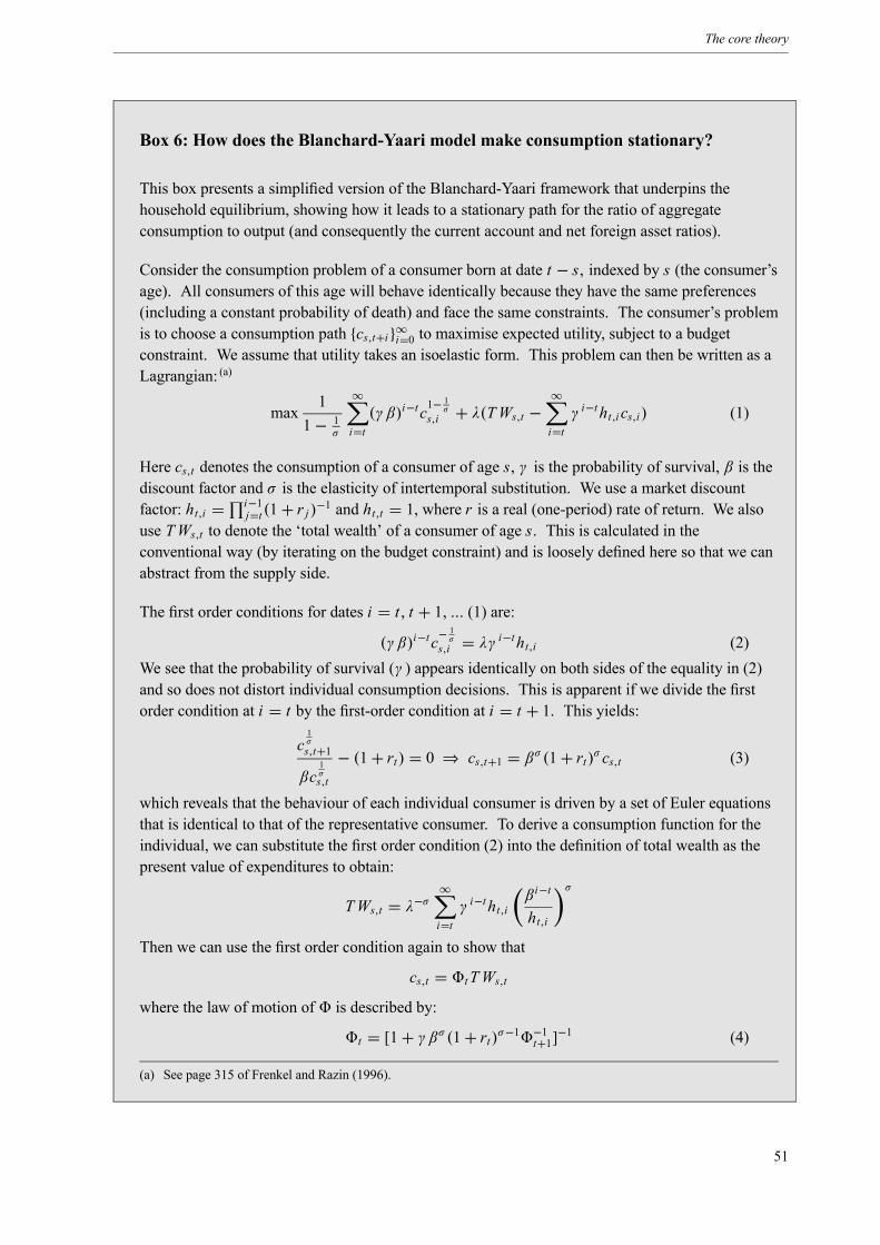
The core theory
Box 6: How does the Blanchard-Yaari model make consumption stationary?
This box presents a simplified version of the Blanchard-Yaari framework that underpins thehousehold equilibrium, showing how it leads to a stationary path for the ratio of aggregateconsumption to output (and consequently the current account and net foreign asset ratios).
Consider the consumption problem of a consumer born at date t − s, indexed by s (the consumer’sage). All consumers of this age will behave identically because they have the same preferences(including a constant probability of death) and face the same constraints. The consumer’s problemis to choose a consumption path {cs,t+i }∞i=0 to maximise expected utility, subject to a budgetconstraint. We assume that utility takes an isoelastic form. This problem can then be written as aLagrangian: (a)
max1
1− 1σ
∞
i=t(γ β)i−t c1−
1σ
s,i + λ(TWs,t −∞
i=tγ i−t ht,i cs,i) (1)
Here cs,t denotes the consumption of a consumer of age s, γ is the probability of survival, β is thediscount factor and σ is the elasticity of intertemporal substitution. We use a market discountfactor: ht,i = i−1
j=t(1+ r j )−1 and ht,t = 1, where r is a real (one-period) rate of return. We alsouse TWs,t to denote the ‘total wealth’ of a consumer of age s. This is calculated in theconventional way (by iterating on the budget constraint) and is loosely defined here so that we canabstract from the supply side.
The first order conditions for dates i = t, t + 1, ... (1) are:(γ β)i−t c−
1σ
s,i = λγ i−t ht,i (2)We see that the probability of survival (γ ) appears identically on both sides of the equality in (2)and so does not distort individual consumption decisions. This is apparent if we divide the firstorder condition at i = t by the first-order condition at i = t + 1. This yields:
c1σs,t+1
βc1σs,t
− (1+ rt) = 0 ⇒ cs,t+1 = βσ (1+ rt)σ cs,t (3)
which reveals that the behaviour of each individual consumer is driven by a set of Euler equationsthat is identical to that of the representative consumer. To derive a consumption function for theindividual, we can substitute the first order condition (2) into the definition of total wealth as thepresent value of expenditures to obtain:
TWs,t = λ−σ∞
i=tγ i−t ht,i
β i−t
ht,i
σ
Then we can use the first order condition again to show that
cs,t = t TWs,t
where the law of motion of is described by:
t = [1+ γβσ (1+ rt)σ−1 −1t+1]
−1 (4)
(a) See page 315 of Frenkel and Razin (1996).
51
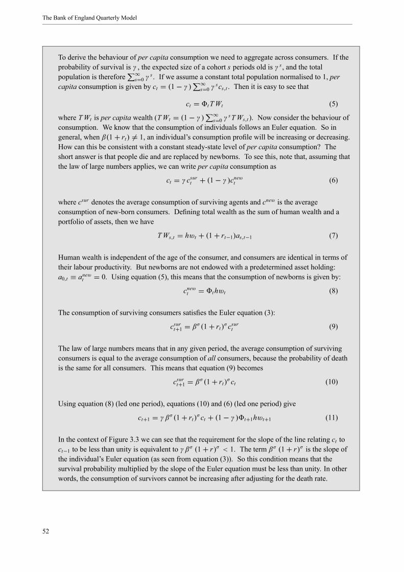
The Bank of England Quarterly Model
To derive the behaviour of per capita consumption we need to aggregate across consumers. If theprobability of survival is γ , the expected size of a cohort s periods old is γ s , and the totalpopulation is therefore ∞
s=0 γ s . If we assume a constant total population normalised to 1, percapita consumption is given by ct = (1− γ ) ∞
s=0 γ scs,t . Then it is easy to see that
ct = t TWt (5)
where TWt is per capita wealth (TWt = (1− γ ) ∞s=0 γ
sTWs,t ). Now consider the behaviour ofconsumption. We know that the consumption of individuals follows an Euler equation. So ingeneral, when β(1+ rt) = 1, an individual’s consumption profile will be increasing or decreasing.How can this be consistent with a constant steady-state level of per capita consumption? Theshort answer is that people die and are replaced by newborns. To see this, note that, assuming thatthe law of large numbers applies, we can write per capita consumption as
ct = γ csurt + (1− γ )cnewt (6)
where csur denotes the average consumption of surviving agents and cnew is the averageconsumption of new-born consumers. Defining total wealth as the sum of human wealth and aportfolio of assets, then we have
TWs,t = hwt + (1+ rt−1)as,t−1 (7)
Human wealth is independent of the age of the consumer, and consumers are identical in terms oftheir labour productivity. But newborns are not endowed with a predetermined asset holding:a0,t ≡ anewt = 0. Using equation (5), this means that the consumption of newborns is given by:
cnewt = t hwt (8)
The consumption of surviving consumers satisfies the Euler equation (3):
csurt+1 = βσ (1+ rt)σcsurt (9)
The law of large numbers means that in any given period, the average consumption of survivingconsumers is equal to the average consumption of all consumers, because the probability of deathis the same for all consumers. This means that equation (9) becomes
csurt+1 = βσ (1+ rt)σ ct (10)
Using equation (8) (led one period), equations (10) and (6) (led one period) give
ct+1 = γβσ (1+ rt)σct + (1− γ ) t+1hwt+1 (11)
In the context of Figure 3.3 we can see that the requirement for the slope of the line relating ct toct−1 to be less than unity is equivalent to γβσ (1+ r)σ < 1. The term βσ (1+ r)σ is the slope ofthe individual’s Euler equation (as seen from equation (3)). So this condition means that thesurvival probability multiplied by the slope of the Euler equation must be less than unity. In otherwords, the consumption of survivors cannot be increasing after adjusting for the death rate.
52
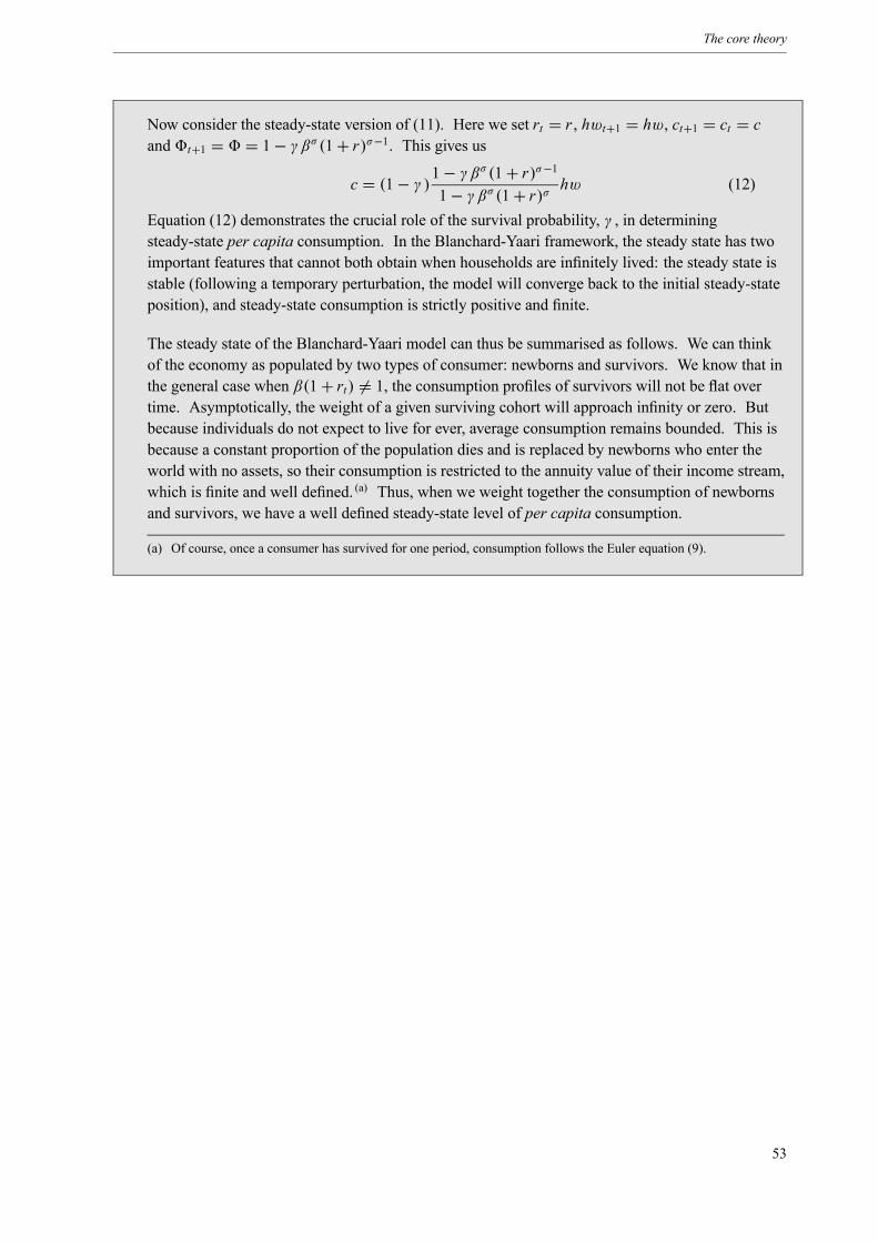
The core theory
Now consider the steady-state version of (11). Here we set rt = r , hwt+1 = hw, ct+1 = ct = cand t+1 = = 1− γβσ (1+ r)σ−1. This gives us
c = (1− γ )1− γβσ (1+ r)σ−1
1− γβσ (1+ r)σ hw (12)
Equation (12) demonstrates the crucial role of the survival probability, γ , in determiningsteady-state per capita consumption. In the Blanchard-Yaari framework, the steady state has twoimportant features that cannot both obtain when households are infinitely lived: the steady state isstable (following a temporary perturbation, the model will converge back to the initial steady-stateposition), and steady-state consumption is strictly positive and finite.
The steady state of the Blanchard-Yaari model can thus be summarised as follows. We can thinkof the economy as populated by two types of consumer: newborns and survivors. We know that inthe general case when β(1+ rt) = 1, the consumption profiles of survivors will not be flat overtime. Asymptotically, the weight of a given surviving cohort will approach infinity or zero. Butbecause individuals do not expect to live for ever, average consumption remains bounded. This isbecause a constant proportion of the population dies and is replaced by newborns who enter theworld with no assets, so their consumption is restricted to the annuity value of their income stream,which is finite and well defined. (a) Thus, when we weight together the consumption of newbornsand survivors, we have a well defined steady-state level of per capita consumption.
(a) Of course, once a consumer has survived for one period, consumption follows the Euler equation (9).
53
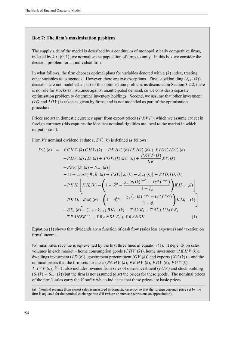
The Bank of England Quarterly Model
Box 7: The firm’s maximisation problem
The supply side of the model is described by a continuum of monopolistically competitive firms,indexed by k ∈ (0, 1); we normalise the population of firms to unity. In this box we consider thedecision problem for an individual firm.
In what follows, the firm chooses optimal plans for variables denoted with a (k) index, treatingother variables as exogenous. However, there are two exceptions. First, stockbuilding (St+i (k))decisions are not modelled as part of this optimisation problem: as discussed in Section 3.2.2, thereis no role for stocks as insurance against unanticipated demand, so we consider a separateoptimisation problem to determine inventory holdings. Second, we assume that other investment(I O and I OV ) is taken as given by firms, and is not modelled as part of the optimisationprocedure.
Prices are set in domestic currency apart from export prices (PXV F), which we assume are set inforeign currency (this captures the idea that nominal rigidities are local to the market in whichoutput is sold).
Firm k’s nominal dividend at date t , DVt (k) is defined as follows:
DVt (k) = PCHVt (k)CHVt (k)+ PK HVt (k) I K HVt (k)+ P I OVt I OVt (k)+PDVt (k) I Dt (k)+ PGVt (k)GVt (k)+ PXV Ft (k)
ERtXVt (k)
+PSVt St (k)− St−1 (k)− (1+ ecostt)Wt Et (k)− PSVt St (k)− St−1 (k) − P I Ot I Ot (k)
−PK Ht K Ht (k)− 1− δkht −χ z zt (k)1+φz − (zss)1+φz
1+ φzK Ht−1 (k)
−PKMt KMt (k)− 1− δkmt − χ z zt (k)1+φz − (zss)1+φz1+ φz
K Mt−1 (k)
+BKt (k)− (1+ rkt−1) BKt−1(k)− T AXKt − T AXLUMPKt−T RANSKCt − T RANSK Ft + T RANSKt (1)
Equation (1) shows that dividends are a function of cash flow (sales less expenses) and taxation onfirms’ income.
Nominal sales revenue is represented by the first three lines of equation (1). It depends on salesvolumes in each market – home consumption goods (CHV (k)), home investment (I K HV (k)),dwellings investment (I D (k)), government procurement (GV (k)) and exports (XV (k)) – and thenominal prices that the firm sets for these (PCHV (k), PK HV (k), PDV (k), PGV (k),PXV F (k)). (a) It also includes revenue from sales of other investment (I OV ) and stock building(St (k)− St−1 (k)) but the firm is not assumed to set the prices for these goods. The nominal pricesof the firm’s sales carry the V suffix which indicates that these prices are basic prices.
(a) Nominal revenue from export sales is measured in domestic currency so that the foreign currency price set by thefirm is adjusted for the nominal exchange rate ER (where an increase represents an appreciation).
54
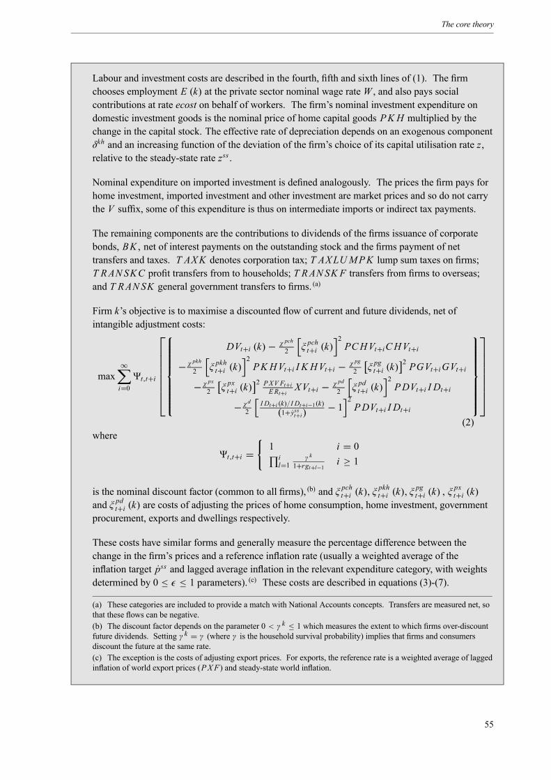
The core theory
Labour and investment costs are described in the fourth, fifth and sixth lines of (1). The firmchooses employment E (k) at the private sector nominal wage rate W , and also pays socialcontributions at rate ecost on behalf of workers. The firm’s nominal investment expenditure ondomestic investment goods is the nominal price of home capital goods PK H multiplied by thechange in the capital stock. The effective rate of depreciation depends on an exogenous componentδkh and an increasing function of the deviation of the firm’s choice of its capital utilisation rate z,relative to the steady-state rate zss .
Nominal expenditure on imported investment is defined analogously. The prices the firm pays forhome investment, imported investment and other investment are market prices and so do not carrythe V suffix, some of this expenditure is thus on intermediate imports or indirect tax payments.
The remaining components are the contributions to dividends of the firms issuance of corporatebonds, BK , net of interest payments on the outstanding stock and the firms payment of nettransfers and taxes. T AXK denotes corporation tax; T AXLUMPK lump sum taxes on firms;T RANSKC profit transfers from to households; T RANSK F transfers from firms to overseas;and T RANSK general government transfers to firms. (a)
Firm k’s objective is to maximise a discounted flow of current and future dividends, net ofintangible adjustment costs:
max∞
i=0t,t+i
⎡⎢⎢⎢⎢⎢⎢⎢⎣
⎧⎪⎪⎪⎪⎪⎪⎪⎨⎪⎪⎪⎪⎪⎪⎪⎩
DVt+i (k)− χ pch
2 ξpcht+i (k)
2PCHVt+iCHVt+i
−χ pkh
2 ξpkht+i (k)
2PK HVt+i I K HVt+i − χ pg
2 ξpgt+i (k)
2 PGVt+iGVt+i
−χ px
2 ξpxt+i (k)
2 PXV Ft+iE Rt+i XVt+i − χ pd
2 ξpdt+i (k)
2PDVt+i I Dt+i
−χd
2I Dt+i (k)/I Dt+i−1(k)
(1+ysst+i)− 1 2
PDVt+i I Dt+i
⎫⎪⎪⎪⎪⎪⎪⎪⎬⎪⎪⎪⎪⎪⎪⎪⎭
⎤⎥⎥⎥⎥⎥⎥⎥⎦(2)
where
t,t+i =1 i = 0il=1
γ k
1+rgt+l−1 i ≥ 1
is the nominal discount factor (common to all firms), (b) and ξ pcht+i (k), ξpkht+i (k), ξ
pgt+i (k) , ξ
pxt+i (k)
and ξ pdt+i (k) are costs of adjusting the prices of home consumption, home investment, governmentprocurement, exports and dwellings respectively.
These costs have similar forms and generally measure the percentage difference between thechange in the firm’s prices and a reference inflation rate (usually a weighted average of theinflation target pss and lagged average inflation in the relevant expenditure category, with weightsdetermined by 0 ≤ ≤ 1 parameters). (c) These costs are described in equations (3)-(7).(a) These categories are included to provide a match with National Accounts concepts. Transfers are measured net, sothat these flows can be negative.(b) The discount factor depends on the parameter 0 < γ k ≤ 1 which measures the extent to which firms over-discountfuture dividends. Setting γ k = γ (where γ is the household survival probability) implies that firms and consumersdiscount the future at the same rate.(c) The exception is the costs of adjusting export prices. For exports, the reference rate is a weighted average of laggedinflation of world export prices (PXF) and steady-state world inflation.
55
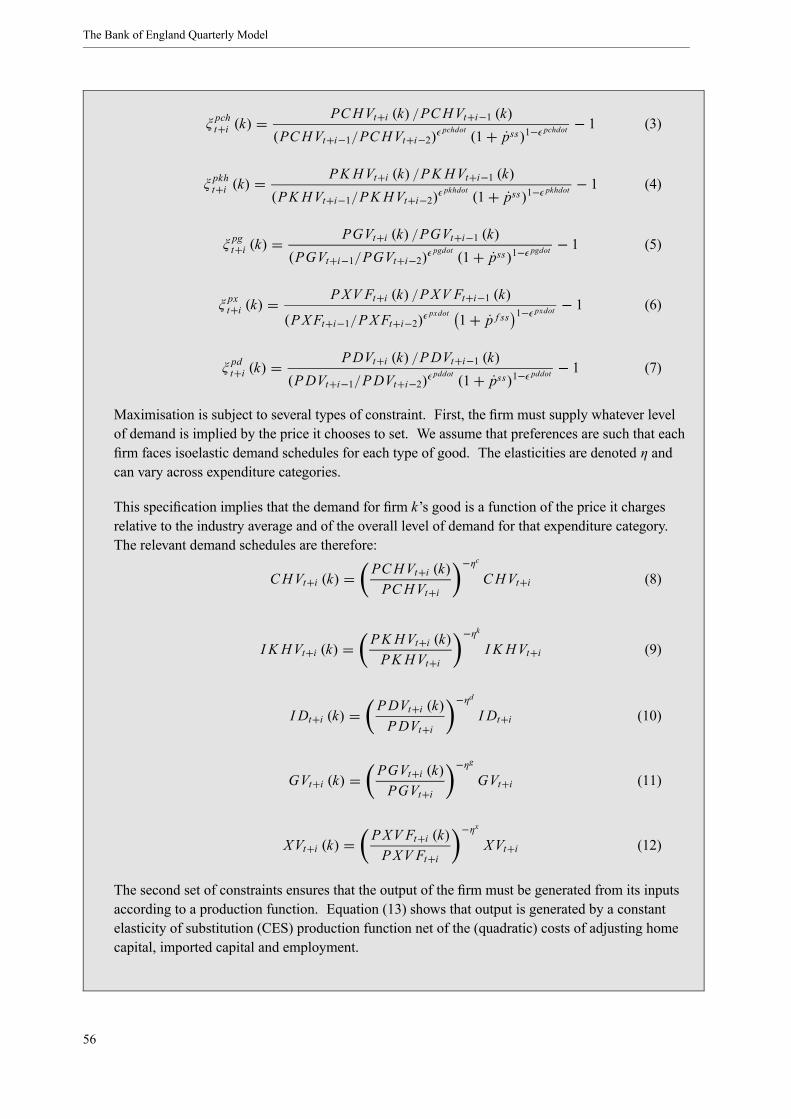
The Bank of England Quarterly Model
ξpcht+i (k) =
PCHVt+i (k) /PCHVt+i−1 (k)(PCHVt+i−1/PCHVt+i−2)
pchdot(1+ pss)1− pchdot − 1 (3)
ξpkht+i (k) =
PK HVt+i (k) /PK HVt+i−1 (k)(PK HVt+i−1/PK HVt+i−2)
pkhdot(1+ pss)1− pkhdot − 1 (4)
ξpgt+i (k) =
PGVt+i (k) /PGVt+i−1 (k)(PGVt+i−1/PGVt+i−2)
pgdot(1+ pss)1− pgdot − 1 (5)
ξpxt+i (k) =
PXV Ft+i (k) /PXV Ft+i−1 (k)
(PXFt+i−1/PXFt+i−2)pxdot 1+ p f ss 1− pxdot − 1 (6)
ξpdt+i (k) =
PDVt+i (k) /PDVt+i−1 (k)(PDVt+i−1/PDVt+i−2)
pddot(1+ pss)1− pddot − 1 (7)
Maximisation is subject to several types of constraint. First, the firm must supply whatever levelof demand is implied by the price it chooses to set. We assume that preferences are such that eachfirm faces isoelastic demand schedules for each type of good. The elasticities are denoted η andcan vary across expenditure categories.
This specification implies that the demand for firm k’s good is a function of the price it chargesrelative to the industry average and of the overall level of demand for that expenditure category.The relevant demand schedules are therefore:
CHVt+i (k) = PCHVt+i (k)PCHVt+i
−ηcCHVt+i (8)
I K HVt+i (k) = PK HVt+i (k)PK HVt+i
−ηkI K HVt+i (9)
I Dt+i (k) = PDVt+i (k)PDVt+i
−ηdI Dt+i (10)
GVt+i (k) = PGVt+i (k)PGVt+i
−ηgGVt+i (11)
XVt+i (k) = PXV Ft+i (k)PXV Ft+i
−ηxXVt+i (12)
The second set of constraints ensures that the output of the firm must be generated from its inputsaccording to a production function. Equation (13) shows that output is generated by a constantelasticity of substitution (CES) production function net of the (quadratic) costs of adjusting homecapital, imported capital and employment.
56
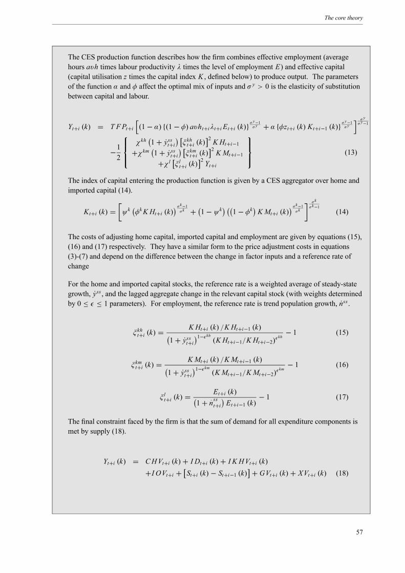
The core theory
The CES production function describes how the firm combines effective employment (averagehours avh times labour productivity λ times the level of employment E) and effective capital(capital utilisation z times the capital index K , defined below) to produce output. The parametersof the function α and φ affect the optimal mix of inputs and σ y > 0 is the elasticity of substitutionbetween capital and labour.
Yt+i (k) = T FPt+i (1− α) {(1− φ) avht+iλt+i Et+i (k)} σy−1σ y + α {φzt+i (k) Kt+i−1 (k)} σ
y−1σ y
σ yσ y−1
−12
⎧⎪⎨⎪⎩χ kh 1+ ysst+i ξ kht+i (k)
2 KHt+i−1+χ km 1+ ysst+i ξ kmt+i (k)
2 KMt+i−1+χ l ξ lt+i (k) 2 Yt+i
⎫⎪⎬⎪⎭ (13)
The index of capital entering the production function is given by a CES aggregator over home andimported capital (14).
Kt+i (k) = ψk φkK Ht+i (k)σ k−1σk + 1− ψk 1− φk KMt+i (k)
σk−1σk
σkσk−1
(14)
The costs of adjusting home capital, imported capital and employment are given by equations (15),(16) and (17) respectively. They have a similar form to the price adjustment costs in equations(3)-(7) and depend on the difference between the change in factor inputs and a reference rate ofchange
For the home and imported capital stocks, the reference rate is a weighted average of steady-stategrowth, yss , and the lagged aggregate change in the relevant capital stock (with weights determinedby 0 ≤ ≤ 1 parameters). For employment, the reference rate is trend population growth, nss .
ξ kht+i (k) =KHt+i (k) /KHt+i−1 (k)
1+ ysst+i 1−kh(KHt+i−1/KHt+i−2)
kh− 1 (15)
ξ kmt+i (k) =KMt+i (k) /KMt+i−1 (k)
1+ ysst+i 1−km(KMt+i−1/KMt+i−2)
km− 1 (16)
ξ lt+i (k) =Et+i (k)
1+ .nsst+i Et+i−1 (k)
− 1 (17)
The final constraint faced by the firm is that the sum of demand for all expenditure components ismet by supply (18).
Yt+i (k) = CHVt+i (k)+ I Dt+i (k)+ I K HVt+i (k)+I OVt+i + St+i (k)− St+i−1 (k) + GVt+i (k)+ XVt+i (k) (18)
57
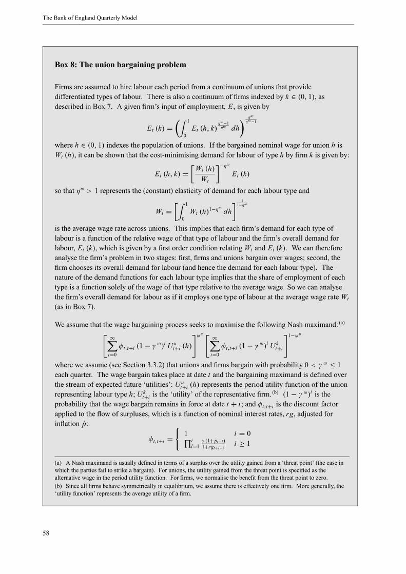
The Bank of England Quarterly Model
Box 8: The union bargaining problem
Firms are assumed to hire labour each period from a continuum of unions that providedifferentiated types of labour. There is also a continuum of firms indexed by k ∈ (0, 1), asdescribed in Box 7. A given firm’s input of employment, E , is given by
Et (k) =1
0Et (h, k)
ηw−1ηw dh
ηw
ηw−1
where h ∈ (0, 1) indexes the population of unions. If the bargained nominal wage for union h isWt (h), it can be shown that the cost-minimising demand for labour of type h by firm k is given by:
Et (h, k) = Wt (h)Wt
−ηwEt (k)
so that ηw > 1 represents the (constant) elasticity of demand for each labour type and
Wt =1
0Wt (h)1−η
wdh
11−ηw
is the average wage rate across unions. This implies that each firm’s demand for each type oflabour is a function of the relative wage of that type of labour and the firm’s overall demand forlabour, Et (k), which is given by a first order condition relating Wt and Et (k). We can thereforeanalyse the firm’s problem in two stages: first, firms and unions bargain over wages; second, thefirm chooses its overall demand for labour (and hence the demand for each labour type). Thenature of the demand functions for each labour type implies that the share of employment of eachtype is a function solely of the wage of that type relative to the average wage. So we can analysethe firm’s overall demand for labour as if it employs one type of labour at the average wage rate Wt(as in Box 7).
We assume that the wage bargaining process seeks to maximise the following Nash maximand: (a)
∞
i=0φt,t+i (1− γ w)i Uut+i (h)
ψu ∞
i=0φt,t+i (1− γ w)i Ukt+i
1−ψu
where we assume (see Section 3.3.2) that unions and firms bargain with probability 0 < γw ≤ 1each quarter. The wage bargain takes place at date t and the bargaining maximand is defined overthe stream of expected future ‘utilities’: Uut+i (h) represents the period utility function of the unionrepresenting labour type h; Ukt+i is the ‘utility’ of the representative firm. (b) (1− γ w)i is theprobability that the wage bargain remains in force at date t + i ; and φt,t+i is the discount factorapplied to the flow of surpluses, which is a function of nominal interest rates, rg, adjusted forinflation p:
φt,t+i =1 i = 0il=1
γ (1+ pt+l )1+rgt+l−1 i ≥ 1
(a) A Nash maximand is usually defined in terms of a surplus over the utility gained from a ‘threat point’ (the case inwhich the parties fail to strike a bargain). For unions, the utility gained from the threat point is specified as thealternative wage in the period utility function. For firms, we normalise the benefit from the threat point to zero.(b) Since all firms behave symmetrically in equilibrium, we assume there is effectively one firm. More generally, the‘utility function’ represents the average utility of a firm.
58
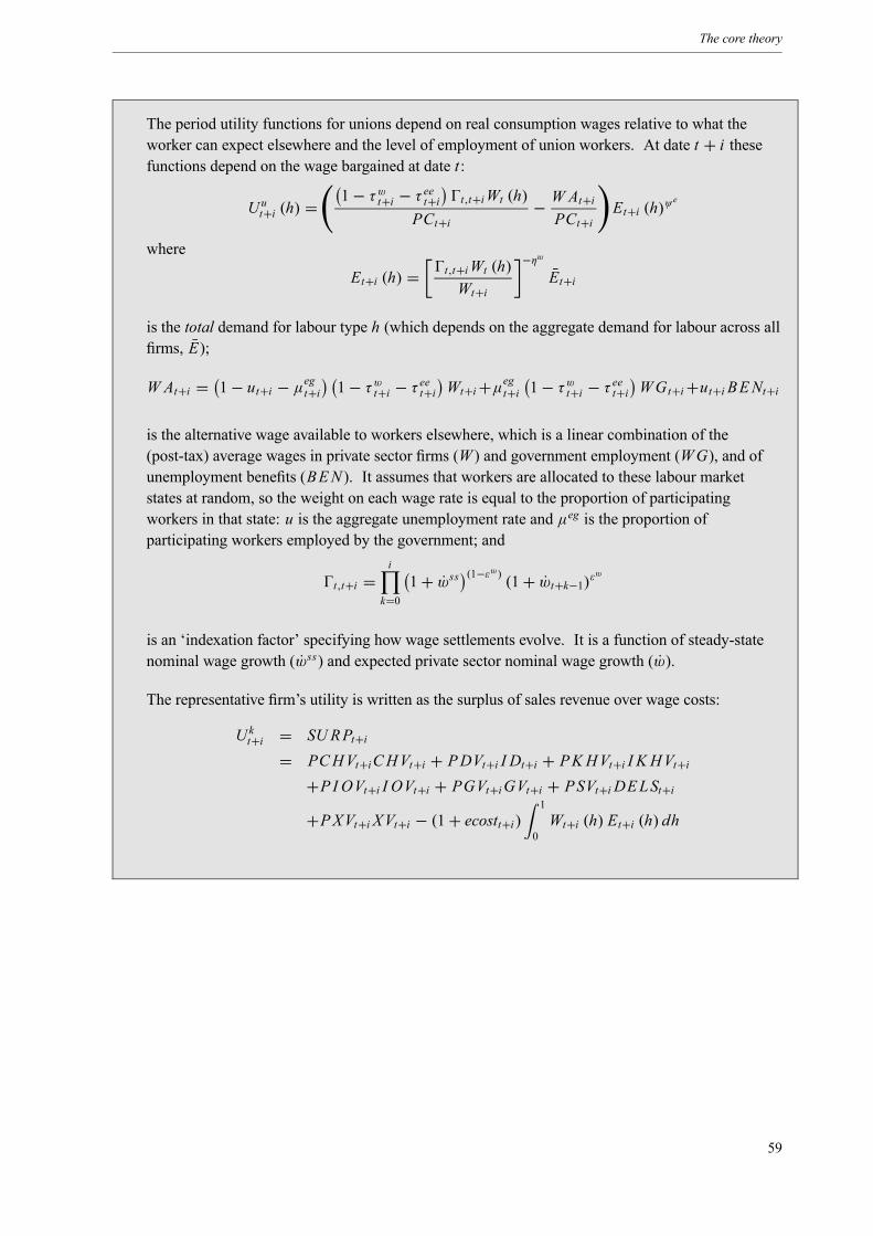
The core theory
The period utility functions for unions depend on real consumption wages relative to what theworker can expect elsewhere and the level of employment of union workers. At date t + i thesefunctions depend on the wage bargained at date t :
Uut+i (h) =1− τwt+i − τ eet+i t,t+iWt (h)
PCt+i− W At+iPCt+i
Et+i (h)ψe
where
Et+i (h) = t,t+iWt (h)Wt+i
−ηwEt+i
is the total demand for labour type h (which depends on the aggregate demand for labour across allfirms, E);
W At+i = 1− ut+i − µegt+i 1− τwt+i − τ eet+i Wt+i+µegt+i 1− τwt+i − τ eet+i WGt+i+ut+i BENt+i
is the alternative wage available to workers elsewhere, which is a linear combination of the(post-tax) average wages in private sector firms (W ) and government employment (WG), and ofunemployment benefits (BEN ). It assumes that workers are allocated to these labour marketstates at random, so the weight on each wage rate is equal to the proportion of participatingworkers in that state: u is the aggregate unemployment rate and µeg is the proportion ofparticipating workers employed by the government; and
t,t+i =i
k=01+ wss (1−εw) (1+ wt+k−1)εw
is an ‘indexation factor’ specifying how wage settlements evolve. It is a function of steady-statenominal wage growth (wss) and expected private sector nominal wage growth (w).
The representative firm’s utility is written as the surplus of sales revenue over wage costs:
Ukt+i = SU RPt+i= PCHVt+iCHVt+i + PDVt+i I Dt+i + PK HVt+i I K HVt+i
+P I OVt+i I OVt+i + PGVt+iGVt+i + PSVt+i DELSt+i+PXVt+i XVt+i − (1+ ecostt+i )
1
0Wt+i (h) Et+i (h) dh
59


Chapter 4 The core/non-core hybrid approach
The previous chapter described the theory behind the structural core model; this chapter explains howwe combine that structural core with ad hoc dynamics and additional variables into one model that wecan use for forecasting, including the application of judgement.
The basic idea behind our approach is simple. The core model embodies a rich economic structure thatcan be used to analyse a wide range of economic issues. Some features in the theoretical structure aredesigned to help match dynamic responses in the data, including the potential for consumption habits,labour adjustment costs, capital and investment adjustment costs, inertia in prices and nominal wages,wage and price inflation stickiness, and slow import price pass-through. However, as discussed inChapter 2, we know that the core model does not fully capture all of the economic channels and dynamicrelationships affecting the observed correlations between economic variables. This in part reflects thechoice not to include in the core model some features of the economy, such as credit market frictions,which could risk making the core model too large and complex to be tractable. Moreover, thetheoretical underpinnings of some aspects of these correlations, for example the degree of persistence ofmany nominal variables, are not yet well understood.
For these reasons, an extra layer of ad hoc ‘non-core’ dynamics is added to reflect additional short-runcorrelations that are not matched by the core theory. For example, we can think of a neoclassical storyfor consumption being combined with proxies for credit effects, or a conventional Jorgensonianuser-cost story for investment supplemented by terms for firms’ gearing in the short run. The full modelis a hybrid combination of core and non-core elements, which matches past movements in the data betterthan either element on its own, and enables a straightforward application of judgement to the forecast.One interpretation of this hybrid approach is that the final projections are a weighted average of threetypes of information: a structural story coming from the core model, extra short-run correlations fromthe non-core model, and judgement applied by the user through the non-core model (the relative weightson these types of information will vary across different parts of the model). Figure 2.2 on page 15shows a stylised example of the forecast process.
A key feature of this approach is the strict separation between the core and non-core elements of themodel. This is reflected in the way that the model is structured, estimated and solved. The need for thisseparation stems from the incompatibility of ad hoc terms with the simultaneous system derived fromthe core theory. As explained in Chapter 3, the decision rules embodied in the core theory are based onthe optimising behaviour of different agents, derived from a set of consistent assumptions aboutpreferences, technology, market conditions etc. As such, it would not be possible to include additionalad hoc terms or to apply judgement to the system without potentially violating the underlyingassumptions, and undermining the theoretical micro-foundations of the decision rules derived fromoptimisation by key agents. (1) This theoretical coherence is central to the ability to use core theory toanalyse various economic issues. Moreover, it is also important in ensuring the stability of thesystem, (2) which is essential in a real-time forecasting context. Hence, BEQM is structured in such a
(1) If we add ad hoc terms to the equations derived from the core theory, it is no longer clear what these equations mean. Thesimultaneity of the core model means that normalisation is arbitrary: adding ad hoc lags to consumption, for example, wouldnot be the same as introducing habit persistence, because habits would be expected to affect the choice of other variables thataffect utility, such as money balances.(2) Experiments with a range of small models have shown that seemingly innocuous additions of own lags and proxy variables,which appear appropriate at the level of an individual equation, can easily create an unstable or wildly oscillating system. Forexample, two sets of ad hoc extensions might ‘work’ by themselves, in the sense that each achieves the desired marginalchange to the system responses, but together they would generate explosive properties or a model that will not always solve.
61
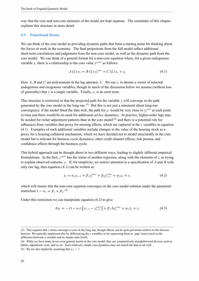
The Bank of England Quarterly Model
way that the core and non-core elements of the model are kept separate. The remainder of this chapterexplains this structure in more detail.
4.1 Functional forms
We can think of the core model as providing dynamic paths that form a starting point for thinking aboutthe forces at work in the economy. The final projections from the full model reflect additionalshort-term correlations and judgement from the non-core model, as well as the dynamic path from thecore model. We can think of a general format for a non-core equation where, for a given endogenousvariable y, there is a relationship to the core value ycore as follows:
A (L) yt = B (L) ycoret + C (L) zt + εt (4.1)
Here A, B and C are polynomials in the lag operator, L. We use zt to denote a vector of selectedendogenous and exogenous variables, though in much of the discussion below we assume (without lossof generality) that z is a single variable. Finally, εt is an error term.
This structure is restricted so that the projected path for the variable y will converge to the pathgenerated by the core model in the long run. (3) But this is not just a statement about long-runconvergence: if the model fitted the data well, the path for yt would be very close to ycoret at each pointin time and there would be no need for additional ad hoc dynamics. In practice, higher-order lags maybe needed for richer adjustment patterns than in the core model (4) and there is a potential role forinfluences from variables that proxy for missing effects, which are captured in the z variables in equation(4.1). Examples of such additional variables include changes in the value of the housing stock as aproxy for a housing collateral mechanism, which we have decided not to model structurally in the coremodel but is relevant for business cycle dynamics; other credit channel effects; risk premia; andconfidence effects through the business cycle.
This hybrid approach can be thought about in two different ways, leading to slightly different empiricalformulations. In the first, ycore has the status of another regressor, along with the elements of z, in tryingto explain observed outturns, y. If, for simplicity, we restrict attention to a specification of A and B withonly one lag, then equation (4.1) can be written as:
yt = α1yt−1 + β1ycoret + β2ycoret−1 + ψ1zt + εt (4.2)
which will ensure that the non-core equation converges on the core model solution under the parameterrestriction 1− α1 = β1 + β2. (5)
Under this restriction we can manipulate equation (4.2) to give:
yt = − (1− α1) yt−1 − ycoret−1 + β1 ycoret + ψ1zt + εt (4.3)
(3) This requires that z terms converge to zero in the long run, though effects can be quite persistent relative to the forecasthorizon. We typically implement this by differencing the z variables or by expressing them as ‘gap’ terms (such as thedifference between a variable and its steady-state level).(4) While we have many levers over general inertia in the core model, they are comparatively straightforward devices such ashabits, adjustment costs, and so on. Such relatively simple core dynamics may not match the data at all well.(5) We are also implicitly assuming that α1 < 1.
62
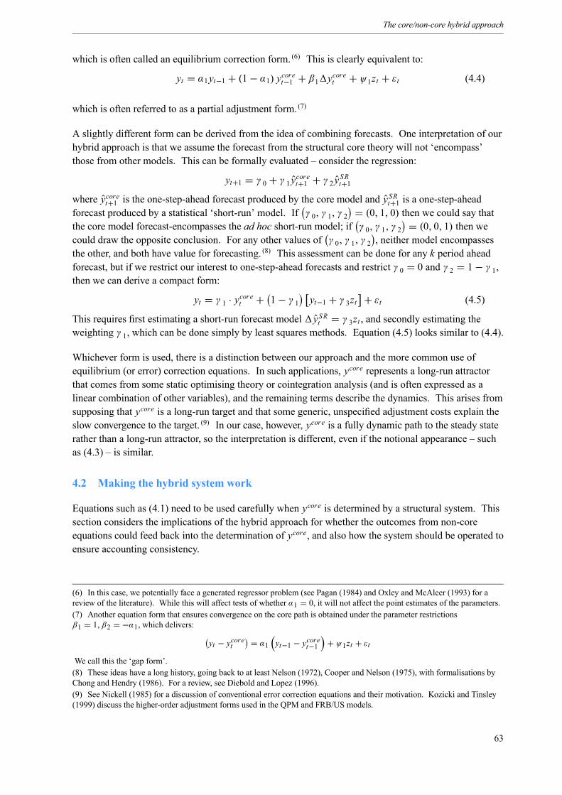
The core/non-core hybrid approach
which is often called an equilibrium correction form. (6) This is clearly equivalent to:
yt = α1yt−1 + (1− α1) ycoret−1 + β1 ycoret + ψ1zt + εt (4.4)
which is often referred to as a partial adjustment form. (7)
A slightly different form can be derived from the idea of combining forecasts. One interpretation of ourhybrid approach is that we assume the forecast from the structural core theory will not ‘encompass’those from other models. This can be formally evaluated – consider the regression:
yt+1 = γ 0 + γ 1 ycoret+1 + γ 2 y SRt+1where ycoret+1 is the one-step-ahead forecast produced by the core model and y
SRt+1 is a one-step-ahead
forecast produced by a statistical ‘short-run’ model. If γ 0, γ 1, γ 2 = (0, 1, 0) then we could say thatthe core model forecast-encompasses the ad hoc short-run model; if γ 0, γ 1, γ 2 = (0, 0, 1) then wecould draw the opposite conclusion. For any other values of γ 0, γ 1, γ 2 , neither model encompassesthe other, and both have value for forecasting. (8) This assessment can be done for any k period aheadforecast, but if we restrict our interest to one-step-ahead forecasts and restrict γ 0 = 0 and γ 2 = 1− γ 1,then we can derive a compact form:
yt = γ 1 · ycoret + 1− γ 1 yt−1 + γ 3zt + εt (4.5)
This requires first estimating a short-run forecast model ySRt = γ 3zt , and secondly estimating theweighting γ 1, which can be done simply by least squares methods. Equation (4.5) looks similar to (4.4).
Whichever form is used, there is a distinction between our approach and the more common use ofequilibrium (or error) correction equations. In such applications, ycore represents a long-run attractorthat comes from some static optimising theory or cointegration analysis (and is often expressed as alinear combination of other variables), and the remaining terms describe the dynamics. This arises fromsupposing that ycore is a long-run target and that some generic, unspecified adjustment costs explain theslow convergence to the target. (9) In our case, however, ycore is a fully dynamic path to the steady staterather than a long-run attractor, so the interpretation is different, even if the notional appearance – suchas (4.3) – is similar.
4.2 Making the hybrid system work
Equations such as (4.1) need to be used carefully when ycore is determined by a structural system. Thissection considers the implications of the hybrid approach for whether the outcomes from non-coreequations could feed back into the determination of ycore, and also how the system should be operated toensure accounting consistency.
(6) In this case, we potentially face a generated regressor problem (see Pagan (1984) and Oxley and McAleer (1993) for areview of the literature). While this will affect tests of whether α1 = 0, it will not affect the point estimates of the parameters.(7) Another equation form that ensures convergence on the core path is obtained under the parameter restrictionsβ1 = 1, β2 = −α1, which delivers:
yt − ycoret = α1 yt−1 − ycoret−1 + ψ1zt + εtWe call this the ‘gap form’.(8) These ideas have a long history, going back to at least Nelson (1972), Cooper and Nelson (1975), with formalisations byChong and Hendry (1986). For a review, see Diebold and Lopez (1996).(9) See Nickell (1985) for a discussion of conventional error correction equations and their motivation. Kozicki and Tinsley(1999) discuss the higher-order adjustment forms used in the QPM and FRB/US models.
63
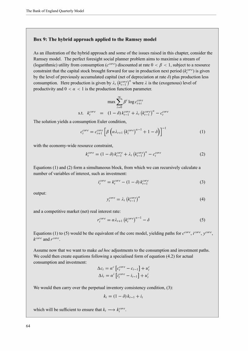
The Bank of England Quarterly Model
Box 9: The hybrid approach applied to the Ramsey model
As an illustration of the hybrid approach and some of the issues raised in this chapter, consider theRamsey model. The perfect foresight social planner problem aims to maximise a stream of(logarithmic) utility from consumption (ccore) discounted at rate 0 < β < 1, subject to a resourceconstraint that the capital stock brought forward for use in production next period (kcoret ) is givenby the level of previously accumulated capital (net of depreciation at rate δ) plus production lessconsumption. Here production is given by λt kcoret−1
α where λ is the (exogenous) level ofproductivity and 0 < α < 1 is the production function parameter.
max∞
i=0β i log ccoret+i
s.t. kcoret = (1− δ) kcoret−1 + λt kcoret−1α − ccoret
The solution yields a consumption Euler condition,
ccoret = ccoret+1 β αλt+1 kcoretα−1 + 1− δ −1
(1)
with the economy-wide resource constraint,
kcoret = (1− δ) kcoret−1 + λt kcoret−1α − ccoret (2)
Equations (1) and (2) form a simultaneous block, from which we can recursively calculate anumber of variables of interest, such as investment:
i coret = kcoret − (1− δ) kcoret−1 (3)
output:ycoret = λt kcoret−1
α (4)
and a competitive market (net) real interest rate:
rcoret = αλt+1 kcoretα−1 − δ (5)
Equations (1) to (5) would be the equivalent of the core model, yielding paths for ccore, i core, ycore,kcore and rcore.
Assume now that we want to make ad hoc adjustments to the consumption and investment paths.We could then create equations following a specialised form of equation (4.2) for actualconsumption and investment:
ct = αc ccoret − ct−1 + uctit = αi i coret − it−1 + uit
We would then carry over the perpetual inventory consistency condition, (3):
kt = (1− δ) kt−1 + it
which will be sufficient to ensure that kt −→ kcoret .
64
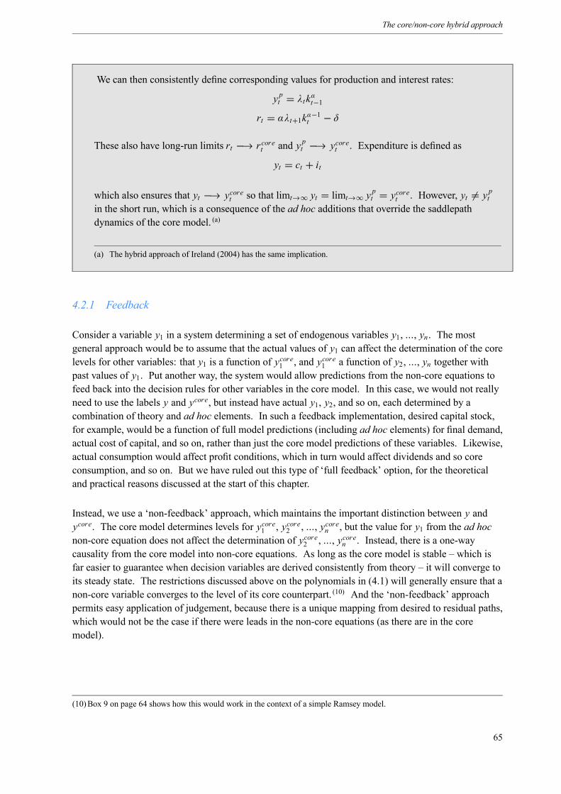
The core/non-core hybrid approach
We can then consistently define corresponding values for production and interest rates:
y pt = λt kαt−1rt = αλt+1kα−1t − δ
These also have long-run limits rt −→ rcoret and y pt −→ ycoret . Expenditure is defined as
yt = ct + it
which also ensures that yt −→ ycoret so that limt→∞ yt = limt→∞ y pt = ycoret . However, yt = y ptin the short run, which is a consequence of the ad hoc additions that override the saddlepathdynamics of the core model. (a)
(a) The hybrid approach of Ireland (2004) has the same implication.
4.2.1 Feedback
Consider a variable y1 in a system determining a set of endogenous variables y1, ..., yn. The mostgeneral approach would be to assume that the actual values of y1 can affect the determination of the corelevels for other variables: that y1 is a function of ycore1 , and ycore1 a function of y2, ..., yn together withpast values of y1. Put another way, the system would allow predictions from the non-core equations tofeed back into the decision rules for other variables in the core model. In this case, we would not reallyneed to use the labels y and ycore, but instead have actual y1, y2, and so on, each determined by acombination of theory and ad hoc elements. In such a feedback implementation, desired capital stock,for example, would be a function of full model predictions (including ad hoc elements) for final demand,actual cost of capital, and so on, rather than just the core model predictions of these variables. Likewise,actual consumption would affect profit conditions, which in turn would affect dividends and so coreconsumption, and so on. But we have ruled out this type of ‘full feedback’ option, for the theoreticaland practical reasons discussed at the start of this chapter.
Instead, we use a ‘non-feedback’ approach, which maintains the important distinction between y andycore. The core model determines levels for ycore1 , ycore2 , ..., ycoren , but the value for y1 from the ad hocnon-core equation does not affect the determination of ycore2 , ..., ycoren . Instead, there is a one-waycausality from the core model into non-core equations. As long as the core model is stable – which isfar easier to guarantee when decision variables are derived consistently from theory – it will converge toits steady state. The restrictions discussed above on the polynomials in (4.1) will generally ensure that anon-core variable converges to the level of its core counterpart. (10) And the ‘non-feedback’ approachpermits easy application of judgement, because there is a unique mapping from desired to residual paths,which would not be the case if there were leads in the non-core equations (as there are in the coremodel).
(10)Box 9 on page 64 shows how this would work in the context of a simple Ramsey model.
65
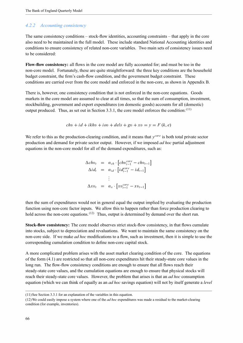
The Bank of England Quarterly Model
4.2.2 Accounting consistency
The same consistency conditions – stock-flow identities, accounting constraints – that apply in the corealso need to be maintained in the full model. These include standard National Accounting identities andconditions to ensure consistency of related non-core variables. Two main sets of consistency issues needto be considered:
Flow-flow consistency: all flows in the core model are fully accounted for; and must be too in thenon-core model. Fortunately, these are quite straightforward: the three key conditions are the householdbudget constraint, the firm’s cash-flow condition, and the government budget constraint. Theseconditions are carried over from the core model and enforced in the non-core, as shown in Appendix B.
There is, however, one consistency condition that is not enforced in the non-core equations. Goodsmarkets in the core model are assumed to clear at all times, so that the sum of consumption, investment,stockbuilding, government and export expenditures (on domestic goods) accounts for all (domestic)output produced. Thus, as set out in Section 3.3.1, the core model enforces the condition: (11)
chv + id + ikhv + iov + dels + gv + xv = y = F (k, e)
We refer to this as the production-clearing condition, and it means that ycore is both total private sectorproduction and demand for private sector output. However, if we imposed ad hoc partial adjustmentequations in the non-core model for all of the demand expenditures, such as:
chvt = αch · chvcoret−1 − chvt−1idt = αid · idcoret−1 − idt−1
...
xvt = αx · xvcoret−1 − xvt−1
then the sum of expenditures would not in general equal the output implied by evaluating the productionfunction using non-core factor inputs. We allow this to happen rather than force production clearing tohold across the non-core equations. (12) Thus, output is determined by demand over the short run.
Stock-flow consistency: The core model observes strict stock-flow consistency, in that flows cumulateinto stocks, subject to depreciation and revaluations. We want to maintain the same consistency on thenon-core side. If we make ad hoc modifications to a flow, such as investment, then it is simple to use thecorresponding cumulation condition to define non-core capital stock.
A more complicated problem arises with the asset market clearing condition of the core. The equationsof the form (4.1) are restricted so that all non-core expenditures hit their steady-state core values in thelong run. The flow-flow consistency conditions are enough to ensure that all flows reach theirsteady-state core values, and the cumulation equations are enough to ensure that physical stocks willreach their steady-state core values. However, the problem that arises is that an ad hoc consumptionequation (which we can think of equally as an ad hoc savings equation) will not by itself generate a level
(11)See Section 3.3.1 for an explanation of the variables in this equation.(12)We could easily impose a system where one of the ad hoc expenditures was made a residual to the market-clearingcondition (for example, inventories).
66
The core/non-core hybrid approach
of cumulated financial wealth that is consistent with the sum of all individual wealth components: theseflows have to integrate to a certain level for full stock-flow consistency to be achieved. In our case, thisinconsistency would be seen in the path of foreign bonds. While the net addition to foreign bonds (aflow) eventually attains the same value as that in the core (as all of the flows in the household budgetconstraint reach their core values), the path of the stock (net foreign assets) could increase or decreasewithout bound. (13)
Our solution for this effectively amounts to a form of integral control in the ad hoc consumptionequation – if non-core consumption is below the core path for a period, then there must be a period of‘over-consumption’ relative to the core in later periods, so that the integral of the implied savings pathmatches the supply of assets. We might think of this as agents being potentially slow to react to apermanent income increase, for a variety of reasons that we do not model in the core (for example,learning, signal extraction, credit constraints), but they eventually make up for short-run mistakes orconstraints. In order to achieve this, we add a term in the asset ‘gap’ to the consumption equation. Astylised representation would be: (14)
B (L) ct = ccoret−1 + ν acoret−1 − at−1 + crest (4.6)
4.2.3 Projections from the hybrid system and the Lucas critique
The hybrid system combines structural and (quasi-) reduced form elements, with relative weightsestimated from the data. As such, the system is vulnerable to the Lucas critique: baseline projectionsusing the system as standard make the implicit assumption that the coefficients on the short-run proxiesand these weights have not shifted. Policy analysis in such a system is therefore made on theassumption that interventions are ‘modest’. (15) However, these coefficients are only a guide. In somecircumstances, they might be imposed. For example, if there were a large shock that might changebehaviour, such as a significant, anticipated change in a distortionary tax, then we might place moreweight on the story from the core model for certain variables.
4.3 Summary
This chapter discusses how the core and non-core models are combined into the full forecasting model.Equations in the core model are based on the optimising behaviour of forward-looking agents, derivedfrom a set of consistent assumptions on factors such as preferences and technology. Non-core equationsinclude additional ad hoc dynamics and variables that proxy for ‘missing’ effects; they also allow directapplication of judgement. The structure of the full model is restricted so that variables must converge tothe long-run paths projected by the core model, but short-term behaviour is potentially quite flexible andamenable to the imposition of judgement.
(13) In the long run, the household budget constraint accumulates foreign bonds at a rate (1+ r) > 1 (where r > 0 is the worldreal interest rate), which is explosive. The consumption path from the core theory ensures that foreign bond holdings do notexplode. But if we impose an alternative consumption path such that consumers ‘overspend’ relative to the core path, thisimplies a lower level of household net assets and, in the absence of any other correction, the level of foreign debt will increasewithout bound. In constrast, physical stocks accumulate at a rate δ < 1, which implies that convergence to a steady-state flowrate ensures a stock level consistent with the steady state of the core model.(14)The size of the coefficient(s) in ν required to ensure that net foreign assets converge to their appropriate steady-state valuewill be determined by the properties (roots) of the system of non-core equations. There is no guarantee that an estimated valuefor ν will ensure convergence – if not, we would need to impose a suitable value.(15)See Leeper and Zha (2001).
67

The Bank of England Quarterly Model
There are a number of benefits from this separation of core and non-core elements. If we introduced thead hoc elements into the core, it would risk violating the underlying theoretical assumptions of the coremodel, and it could also produce an unstable system. One way of viewing this hybrid approach is thatthe path from the core model is treated as a regressor, along with additional variables and ad hocdynamics, in the full model equation.
We do not allow projections from non-core equations to feed back into the core model, which wouldbring about similar problems of instability and an undermining of the micro-foundations of the coretheory. Instead we use a ‘non-feedback’ approach, which maintains the distinction between the valuesfrom the core and the full forecasting models: there is one-way causality from the core model to thenon-core equations. This also facilitates the direct application of judgement to the forecast model, sothat it is easy to impose desired paths for particular variables. In the full model, we generally impose thesame stock-flow and flow-flow consistency conditions as in the core model. An exception is that outputis determined by demand in the short term.
68
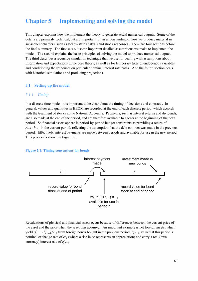
Chapter 5 Implementing and solving the model
This chapter explains how we implement the theory to generate actual numerical outputs. Some of thedetails are primarily technical, but are important for an understanding of how we produce material insubsequent chapters, such as steady-state analysis and shock responses. There are four sections beforethe final summary. The first sets out some important detailed assumptions we make to implement themodel. The second explains the basic principles of solving the model to produce numerical outputs.The third describes a recursive simulation technique that we use for dealing with assumptions aboutinformation and expectations in the core theory, as well as for temporary fixes of endogenous variablesand conditioning the responses on particular nominal interest rate paths. And the fourth section dealswith historical simulations and producing projections.
5.1 Setting up the model
5.1.1 Timing
In a discrete time model, it is important to be clear about the timing of decisions and contracts. Ingeneral, values and quantities in BEQM are recorded at the end of each discrete period, which accordswith the treatment of stocks in the National Accounts. Payments, such as interest returns and dividends,are also made at the end of the period, and are therefore available to agents at the beginning of the nextperiod. So financial assets appear in period-by-period budget constraints as providing a return ofrt−1 · bt−1 in the current period, reflecting the assumption that the debt contract was made in the previousperiod. Effectively, interest payments are made between periods and available for use in the next period.This process is shown in Figure 5.1.
Figure 5.1: Timing conventions for bonds
t -1 t
record value for bond stock at end of period
interest payment made
value (1+r t -1)·b t -1
available for use in period t
investment made in new bonds
record value for bond stock at end of period
Revaluations of physical and financial assets occur because of differences between the current price ofthe asset and the price when the asset was acquired. An important example is net foreign assets, whichyield rf t−1 · bf t−1/ert from foreign bonds bought in the previous period, bf t−1, valued at this period’snominal exchange rate of ert (where a rise in er represents an appreciation) and carry a real (owncurrency) interest rate of rf t−1.
69
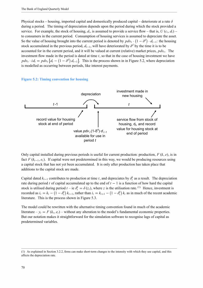
The Bank of England Quarterly Model
Physical stocks – housing, imported capital and domestically produced capital – deteriorate at a rate δduring a period. The timing of depreciation depends upon the period during which the stock provided aservice. For example, the stock of housing, dt , is assumed to provide a service flow – that is, U (ct , dt) –to consumers in the current period. Consumption of housing services is assumed to depreciate the asset.So the value of housing brought into the current period is denoted by pdvt · 1− δd · dt−1: the housingstock accumulated in the previous period, dt−1, will have deteriorated by δd by the time it is to beaccounted for in the current period, and it will be valued at current (relative) market prices, pdvt . Theinvestment flow made in the period is dated at time t , so that in the case of housing investment we havepdvt · idt = pdvt dt − 1− δd dt−1 . This is the process shown in in Figure 5.2, where depreciationis modelled as occurring between periods, like interest payments.
Figure 5.2: Timing convention for housing
t -1 t
record value for housing stock at end of period
depreciation
value pdv t (1-δd)·d t -1
available for use in period t
investment made in new housing
service flow from stock of housing, dt, and record
value for housing stock at end of period
Only capital installed during previous periods is useful for current production: production, F (k, e), is infact F (kt−1, et). If capital were not predetermined in this way, we would be producing resources usinga capital stock that has not yet been accumulated. It is only after production has taken place thatadditions to the capital stock are made.
Capital dated kt−1 contributes to production at time t , and depreciates by δkt as a result. The depreciationrate during period t of capital accumulated up to the end of t − 1 is a function of how hard the capitalstock is utilised during period t – ie δkt = δ (zt), where z is the utilisation rate. (1) Hence, investment isrecorded as it = kt − 1− δkt kt−1, rather than it = kt+1− 1− δkt kt as in much of the recent academicliterature. This is the process shown in Figure 5.3.
The model could be rewritten with the alternative timing convention found in much of the academicliterature – yt = F (kt , et) – without any alteration to the model’s fundamental economic properties.But our notation makes it straightforward for the simulation software to recognise lags of capital aspredetermined variables.
(1) As explained in Section 3.2.2, firms can make short-term changes to the intensity with which they use capital, and thisaffects the depreciation rate.
70
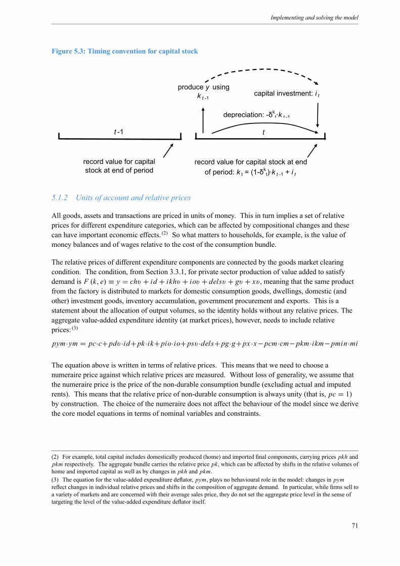
Implementing and solving the model
Figure 5.3: Timing convention for capital stock
t -1 t
record value for capital stock at end of period
depreciation: -δkt·k t -1
produce y using k t -1
capital investment: i t
record value for capital stock at end of period: k t = (1-δk
t)·k t -1 + i t
5.1.2 Units of account and relative prices
All goods, assets and transactions are priced in units of money. This in turn implies a set of relativeprices for different expenditure categories, which can be affected by compositional changes and thesecan have important economic effects. (2) So what matters to households, for example, is the value ofmoney balances and of wages relative to the cost of the consumption bundle.
The relative prices of different expenditure components are connected by the goods market clearingcondition. The condition, from Section 3.3.1, for private sector production of value added to satisfydemand is F (k, e) ≡ y = chv + id + ikhv + iov + delsv + gv + xv , meaning that the same productfrom the factory is distributed to markets for domestic consumption goods, dwellings, domestic (andother) investment goods, inventory accumulation, government procurement and exports. This is astatement about the allocation of output volumes, so the identity holds without any relative prices. Theaggregate value-added expenditure identity (at market prices), however, needs to include relativeprices: (3)
pym ·ym = pc·c+pdv ·id+pk ·ik+pio·io+psv ·dels+pg·g+px ·x−pcm ·cm−pkm ·ikm−pmin·mi
The equation above is written in terms of relative prices. This means that we need to choose anumeraire price against which relative prices are measured. Without loss of generality, we assume thatthe numeraire price is the price of the non-durable consumption bundle (excluding actual and imputedrents). This means that the relative price of non-durable consumption is always unity (that is, pc = 1)by construction. The choice of the numeraire does not affect the behaviour of the model since we derivethe core model equations in terms of nominal variables and constraints.
(2) For example, total capital includes domestically produced (home) and imported final components, carrying prices pkh andpkm respectively. The aggregate bundle carries the relative price pk, which can be affected by shifts in the relative volumes ofhome and imported capital as well as by changes in pkh and pkm.(3) The equation for the value-added expenditure deflator, pym, plays no behavioural role in the model: changes in pymreflect changes in individual relative prices and shifts in the composition of aggregate demand. In particular, while firms sell toa variety of markets and are concerned with their average sales price, they do not set the aggregate price level in the sense oftargeting the level of the value-added expenditure deflator itself.
71
The Bank of England Quarterly Model
5.1.3 Stationarity
We find it convenient to have a stationary model in which the steady state can be expressed as a series ofconstant values measured in ‘detrended model units’ (see Chapter 6). This means that policy simulationsand comparative static experiments are computationally simple, fast and straightforward to run. Forprojections, this structure means that it is easy to make consistent changes to trend growth assumptions.
Because the model settles on a balanced-growth path (meaning that variables grow at constant, commonrates in the steady state), we can write the model in a stationary form by scaling any given variable bythe appropriate trend growth rate. In general, therefore, a lagged variable will need to be scaled down bythe growth rate, and a lead variable will be correspondingly scaled up (see Box 12 on page 88). Whenthe model is solved, rescaling to levels is a simple cumulation conversion, given a starting point for eachvariable. For most real variables, such as goods and assets, the appropriate scaling is the growth rate ofproductive potential, 1+ y. For human wealth, transfer wealth, variables associated with the wageschedule and labour values, the appropriate scaling is by labour productivity growth, 1+ λ. For nominalvariables, scaling is by the rate of inflation in the numeraire price, 1+ p.
5.1.4 Linearity
A standard approach in much of the DSGE literature is to linearise around the non-stochastic steadystate and then to solve for the rational expectation of the endogenous variables. Instead, we leave themodel in levels, which allows us to analyse how permanent shocks affect the steady state. We use asolution method that can handle systems of non-linear difference equations (see Section 5.2). Thenon-linearity implies that the movement of the model to a new steady-state equilibrium can beinfluenced by the starting point. (4)
There are, however, some potential costs to working with a non-linear model. First, care is neededbecause model responses are now dependent on the starting point and the size of the shock. Second,non-linearity makes numerical convergence problems more likely. Third, some exercises require alinear model – for example, conventional classical control exercises. Fortunately, numerical calculationof a linearised version for such purposes is relatively straightforward.
5.1.5 Expectations in the core model
Equations in the core model have leads as well as lags and are derived under the assumption that agentsknow how the paths for endogenous variables are determined from the expected evolution of exogenousvariables. This, combined with the assumption that agents form point expectations about futureexogenous variables, implies that the model can be treated as deterministic. (5) Formally, suppose that yrepresents endogenous variables and x represents exogenous variables. If all agents know the model andthe past histories of endogenous and exogenous variables yt− j , xt− j
∞j=0; and they have point
expectations for the future paths of exogenous variables xt+ j∞j=1, then their expectations of future
endogenous variables coincide with the core model solutions generated by those paths. Suchexpectations are often referred to as model-consistent.
(4) A good example is the pure wealth effects that arise as a result of the Blanchard-Yaari paradigm for the household: anincrease in the supply of government debt will make households rebalance their asset portfolios, including net foreign assetlevels, necessitating a current account and real exchange rate response. The extent of these responses will depend on the netforeign asset position at the starting point. See Chapter 7 of Frenkel and Razin (1996).(5) Point expectations mean that agents place full probability on a particular path for exogenous variables. An implication isthat certainty equivalence holds. See pages 57-59 of Sargent and Ljungqvist (2000) for a formal definition.
72
Implementing and solving the model
This might appear different to the conventional approach usually taken in DSGE models, where agentsknow only current and past y and x : yt− j , xt− j
∞j=0. However, that approach also implies model
consistent expectations, as is made clear in King, Plosser and Rebelo (1988). The difference is that,under that approach, simplifying assumptions are made about the nature of the processes determiningthe exogenous variables, so that an equilibrium can be calculated from knowledge of y and x only up totime t .
We do not follow the standard DSGE approach for practical reasons. In the conventional linear DSGEapproach, expectations of future exogenous variables are solved out by assuming that these variablesfollow simple autoregressive processes. Unfortunately, real-world forecasting issues are usually morecomplex. For example, we would want to condition on exogenous paths for fiscal plans – taxes,transfers, spending – that may have been pre-announced and will almost certainly not follow simpleautoregressive processes. Much of forecasting involves changing assumptions about the present andfuture processes determining exogenous variables to see what happens to the endogenous variables –which means that we need to be able to manipulate future exogenous variables directly. This is possiblein the DSGE approach, but would require constructing auxiliary equations for expectations of a variablefor each period in the future (and having to change these equations when expectational assumptionschange). (6) In our case, assumptions about future paths of exogenous variables are a frequent issue inforecasts (see Section 5.3), which require a more flexible approach.
The assumption of model-consistent expectations has been a standard assumption in macroeconomicmodelling for some time, often combined with the additional assumption that agents have fullinformation about the future paths of exogenous variables (including shocks hitting the economy). It isnot intended as a realistic description, and there are sometimes cases where we would like a tractablemeans of imposing an alternative assumption. One model of learning is that of Erceg and Levin (2003),in which agents use a filter to extract signals about the true persistence of the shocks hitting the economy.Agents may have to decide, for example, to what extent an observed change in world demand representsa temporary shock or a permanent change. Such a model of learning could easily be implemented usingthe recursive simulation methodology (described in Section 5.3) which allows us to specify how pointexpectations of future exogenous variables are falsified by a sequence of unanticipated shocks.
5.1.6 Stability analysis
The conditions for stability for linear rational expectations models are laid out in the well-known paperby Blanchard and Kahn (1980). Essentially, the analysis rests on the eigenvalues of the system, so itcannot be applied directly to non-linear systems. However, we can get some information from a systemlinearised around a point, such as the steady state. Our linearisation procedures rely on the fact that thesaddlepath dynamics of the non-linear model are well described by the dynamics of a linearapproximation close to the steady state. (7) Subject to this caveat, the Blanchard and Kahn conditions aresatisfied for our model.
(6) See Cochrane (1993) for an illustration.(7) The extent to which the saddlepath dynamics are well approximated by the linearised model is discussed by Anderson(1999).
73

The Bank of England Quarterly Model
5.2 Solving the model
This section explains the basics of solving the model. As discussed in previous chapters, the model ismade up of two distinct parts. The core model is forward looking, which raises special issues in termsof producing numerical solutions: much of the discussion below concerns the technicalities of solvingthe core model. In contrast, the full model takes the core model as given and adds backward-looking(non-core) dynamics. Since the non-core equations are backward looking, the full model can be solvedwith conventional techniques for systems of simultaneous equations, conditional on a solution for thecore model.
The basic requirements are easy to describe: we need a set of starting values and a set of internallyconsistent terminal values, together with a method to solve for paths connecting the two sets of pointsthat are consistent with the structure of the model. Before addressing these three issues, however, wefirst address how to solve for the steady state.
5.2.1 Solving the steady state
The solution to the steady state of the complete model is the long-run equilibrium implied by the coretheory. As the core model is designed to follow a balanced-growth path, we can write both the core andnon-core models in stationary form. This makes solving the steady state considerably easier, as thesolution to the steady state is defined by a set of constant values, given assumptions for world anddomestic inflation, domestic labour productivity and population growth. By stripping out leads and lagsfrom the core model, we can create a separate steady-state model. This is solved directly as astraightforward simultaneous equations problem. The results for steady-state ratios will often be ofdirect interest (such as when looking at comparative statics); using this approach we can solve thesteady-state model without any need to solve the full dynamic model forward.
5.2.2 Starting values
We need to know where the system is starting from to solve for the dynamics of the model. Inparticular, we need values for the system’s predetermined (ie lagged endogenous) variables. There aretwo alternatives: we can shock the model from an initial steady-state equilibrium that we have solved foras described above; or for forecasting, we can supply the model with current and historical values for thepredetermined variables. In the latter case, the ‘shocks’ are implicit in the fact that the system isassumed to be away from its long-run equilibrium, and the model’s responses show how the system getsto this equilibrium.
5.2.3 Terminal values
The assumption of model-consistent expectations means that some equations contain leads as well aslags, so we need to have a set of terminal conditions: a solution for up to time T requires values for theleads at T + 1. We use the solution to the steady-state model to define the values of these terminalconditions. When a temporary shock is applied to the model starting from a steady-state equilibrium,the terminal conditions will be those same starting conditions. For a permanent shock, we have tocalculate new steady-state levels, which are derived by solving the steady-state model under the newassumptions. (8)
(8) The decision rules of the core model are expressed in levels, because we are often interested in what happens when there isa new steady state. In contrast, it is common in the conventional DSGE approach to solve for a steady-state equilibrium, andthen derive a recursive law of motion for state variables, given linearised decision rules for the endogenous variables as
74

Implementing and solving the model
5.2.4 Solving the model dynamically
We need a procedure to reconcile leads and lags for a set of non-linear difference equations, from aknown starting point (the predetermined variables), to reach terminal conditions at T + 1 – a problem ofthe form Yt = f (Yt+1,Yt−1). We use the popular Stacked Time algorithm of Laffargue (1990),Boucekkine (1995) and Juillard (1996); the LBJ algorithm appears in practice to be faster and morereliable than ‘first-order’ methods. (9)
Nonetheless, despite the significant recent advances in solution algorithms and computing power, theremay still be situations where we fail to find a solution. Typically a valid solution will exist, but it maybe difficult or impossible for the solution algorithm to locate it, given the initial conditions. This canarise when the starting point is a long way from the desired steady state (as can happen in a forecastcontext) or the shock is large or ‘unusual’.
In such cases our approach is to solve a linearised model dynamically in order to derive a series ofguesses for future values of endogenous variables from the starting point. The linearisation is performednumerically around the appropriate steady state. We find that this approach substantially increasesreliability and reduces total simulation times, even though we have to solve another model.
5.3 Recursive simulations
In a standard simulation experiment with a model such as BEQM, we would shock the model from aninitial starting point and record the solution to the terminal condition, deriving the entire path for eachendogenous variable. But many of the exercises we want to conduct with the model do not necessarilysuit this approach. In particular, in a standard simulation, any future changes to exogenous variablesafter the initial shock are assumed to be fully anticipated. In contrast, we may want to be able tosimulate a sequence of unanticipated shocks, especially if analysing how the response of the economy isaffected by the degree to which agents anticipate future events. But how should we think ofimplementing an unanticipated shock that takes place some time in the future?
We can change the degree to which agents anticipate future events by using the technique of recursivesimulations. The basic idea is simple: if we are dealing with an exogenous variable that is potentiallysubject to shocks in each future period, instead of describing the entire path of all variables by the resultsfrom a single, one-shot projection, we build up a profile in which information about exogenous variablesis revealed period by period. The paths of endogenous variables will change as more information aboutexogenous variables is revealed.
We start the forecast by solving the model at period t . That result for the endogenous variables at t + 1is used as the starting point for a new projection at t + 1, which incorporates one more period’sinformation about the exogenous variables, and the model is solved again with the endogenous variablesfrom that used as the starting point for period t + 2. We continue the process period by period until wehave a complete profile. (10)
The following subsections illustrate where this approach is useful.
deviations from that steady state. In that case, the model would return to the steady-state equilibrium following a shock (aslong as implicit transversality conditions are observed in the theory and the appropriate policy rules are stabilising).(9) See, inter alia, Judd (2002).(10)At some arbitrary period t + j < T in the future, we would be content to run the model out to period T .
75
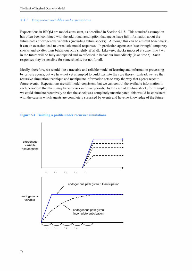
The Bank of England Quarterly Model
5.3.1 Exogenous variables and expectations
Expectations in BEQM are model-consistent, as described in Section 5.1.5. This standard assumptionhas often been combined with the additional assumption that agents have full information about thefuture paths of exogenous variables (including future shocks). Although this can be a useful benchmark,it can on occasion lead to unrealistic model responses. In particular, agents can ‘see through’ temporaryshocks and so alter their behaviour only slightly, if at all. Likewise, shocks imposed at some time t + iin the future will be fully anticipated and so reflected in behaviour immediately (ie at time t). Suchresponses may be sensible for some shocks, but not for all.
Ideally, therefore, we would like a tractable and reliable model of learning and information processingby private agents, but we have not yet attempted to build this into the core theory. Instead, we use therecursive simulation technique and manipulate information sets to vary the way that agents react tofuture events. Expectations are still model-consistent, but we can control the available information ineach period, so that there may be surprises in future periods. In the case of a future shock, for example,we could simulate recursively so that the shock was completely unanticipated: this would be consistentwith the case in which agents are completely surprised by events and have no knowledge of the future.
Figure 5.4: Building a profile under recursive simulations
endogenousvariable
t 0 t +1 t +2 t +3 t +4
endogenous path given incomplete anticipation
exogenousvariable
assumptions
t 0 t +1 t +2 t +3 t +4
endogenous path given full anticipation
76

Implementing and solving the model
A stylised representation of the different responses this approach can lead to is given in Figure 5.4. Theblue lines show a path for an exogenous variable in the top panel and the associated path for a givenendogenous variable under full anticipation in the bottom panel. (11) The dashed lines in the top panelshow a sequence of paths such that only partial information is given about the future path of theexogenous variable – the first line in period t0, the second in period t1 and so on. The dashed line in thebottom panel shows the result of linking the series of jumps each period under the sequence ofexogenous paths shown in the top panel. We have an auxiliary model – the exogenous variables model –that allows us to vary the degree of anticipation of each exogenous variable between the two extremes ofcomplete anticipation and complete surprise (see Box 10 on page 78).
5.3.2 Imposing judgement directly on endogenous variables
The preceding section showed how recursive simulations can be used to vary the assumptions about theinformation available to agents at different points in time, and how this affects the path of endogenousvariables. Here we consider a different issue, involving direct manipulation of endogenous variables.On some occasions, such as in a forecast, we may wish to apply judgement directly onto an endogenousvariable, for example to take account of ‘off-model’ theories or data.
The forward-looking nature of the core model implies that adjusting core model solutions by applyingresiduals (or shocks) to particular equations is not straightforward. In principle, it is possible to‘exogenise’ an endogenous variable temporarily. (12) The model will solve as before, but it will beconditioned on the path for the temporarily ‘exogenised’ variable. However, we quickly encounterproblems with this approach. The first is purely numerical: the model might not solve for a path that istoo long or too far away from the stable path (or saddlepath) for the endogenous variable. Secondly,forward-looking behaviour implies that current variables will be stabilised by expected future marketclearing conditions, so exogenising variables that have to ensure future stabilisation can generate currentinstability. Finally, even if the model can solve for the temporary ‘fix’, the path will be fully anticipatedand private agents will make decisions at time t in anticipation of the end of the fix. Hence, even if thefix can be executed, the results may not be a good match to the thought experiment in mind.
Instead, we simulate recursively so that an endogenous variable may be fixed for a single period, movingforward with each successive simulation. Single-period fixes are computationally much easier for thesimulation software to handle, and recursive simulations allow us to trace out virtually any desired pathas a series of one-period unanticipated fixes. (13) The story consistent with this technique is that agentsare successively surprised with outturns for an endogenous variable, which differ from their ownmodel-consistent forecasts. Box 11 on page 80 provides an example of this approach in terms of fixinga path for the short-term nominal interest rate.
(11) In practice, we would expect dynamics to be much richer than shown here; for clarity we assume that the endogenousvariable jumps from its starting point immediately when the shock is known.(12)Technically, we apply a shock term to an equation in the core model to deliver a particular path for an endogenousvariable, conditioned on the profiles of all other shocks in the model. In other words, we find a sequence of shocks to themodel that deliver a particular profile for an endogenous variable as an equilibrium. This is not equivalent to making thevariable truly exogenous, in the sense that all agents in the model understand that the variable will follow the particular pathindependently of the profiles of other shocks.(13)Numerical problems may still arise if we suppress the model’s natural dynamic reaction for so many periods that it movesfar away from steady-state equilibrium.
77
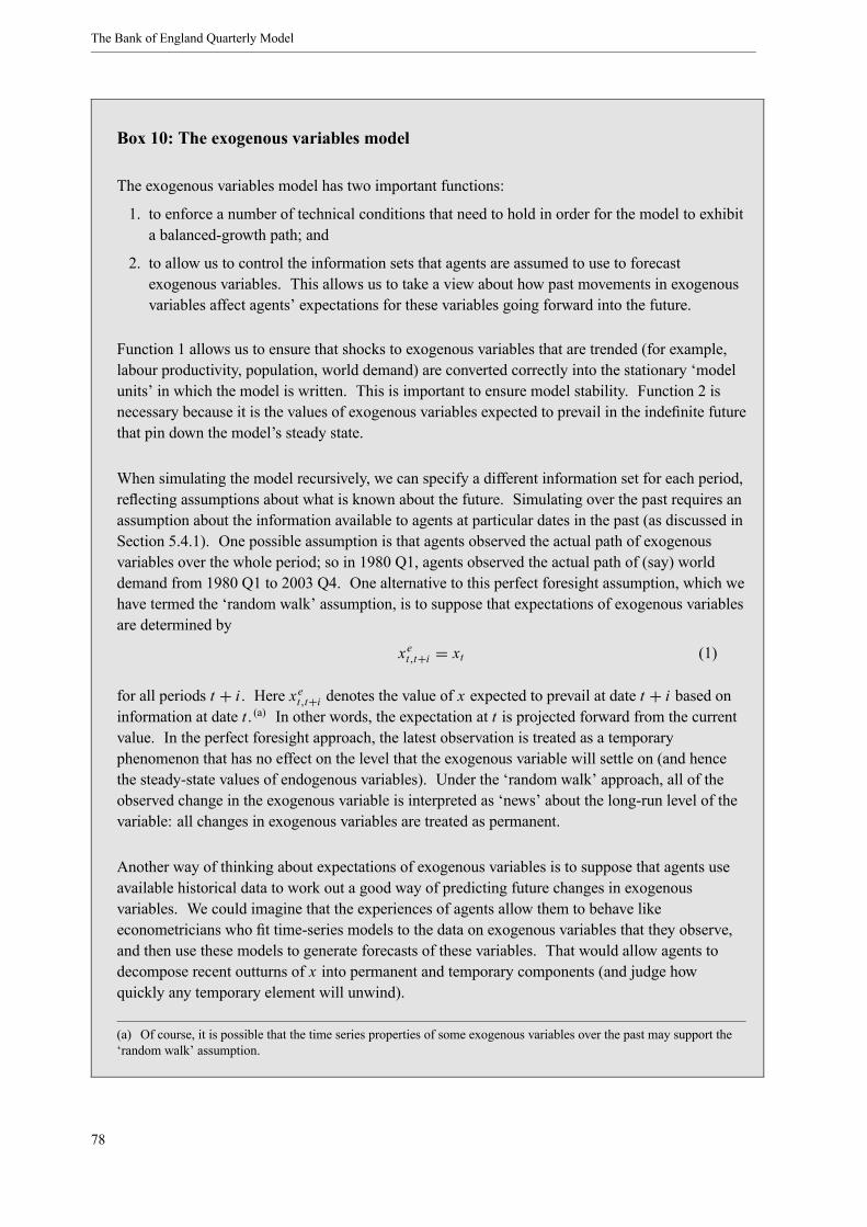
The Bank of England Quarterly Model
Box 10: The exogenous variables model
The exogenous variables model has two important functions:
1. to enforce a number of technical conditions that need to hold in order for the model to exhibita balanced-growth path; and
2. to allow us to control the information sets that agents are assumed to use to forecastexogenous variables. This allows us to take a view about how past movements in exogenousvariables affect agents’ expectations for these variables going forward into the future.
Function 1 allows us to ensure that shocks to exogenous variables that are trended (for example,labour productivity, population, world demand) are converted correctly into the stationary ‘modelunits’ in which the model is written. This is important to ensure model stability. Function 2 isnecessary because it is the values of exogenous variables expected to prevail in the indefinite futurethat pin down the model’s steady state.
When simulating the model recursively, we can specify a different information set for each period,reflecting assumptions about what is known about the future. Simulating over the past requires anassumption about the information available to agents at particular dates in the past (as discussed inSection 5.4.1). One possible assumption is that agents observed the actual path of exogenousvariables over the whole period; so in 1980 Q1, agents observed the actual path of (say) worlddemand from 1980 Q1 to 2003 Q4. One alternative to this perfect foresight assumption, which wehave termed the ‘random walk’ assumption, is to suppose that expectations of exogenous variablesare determined by
xet,t+i = xt (1)
for all periods t + i . Here xet,t+i denotes the value of x expected to prevail at date t + i based oninformation at date t . (a) In other words, the expectation at t is projected forward from the currentvalue. In the perfect foresight approach, the latest observation is treated as a temporaryphenomenon that has no effect on the level that the exogenous variable will settle on (and hencethe steady-state values of endogenous variables). Under the ‘random walk’ approach, all of theobserved change in the exogenous variable is interpreted as ‘news’ about the long-run level of thevariable: all changes in exogenous variables are treated as permanent.
Another way of thinking about expectations of exogenous variables is to suppose that agents useavailable historical data to work out a good way of predicting future changes in exogenousvariables. We could imagine that the experiences of agents allow them to behave likeeconometricians who fit time-series models to the data on exogenous variables that they observe,and then use these models to generate forecasts of these variables. That would allow agents todecompose recent outturns of x into permanent and temporary components (and judge howquickly any temporary element will unwind).
(a) Of course, it is possible that the time series properties of some exogenous variables over the past may support the‘random walk’ assumption.
78

Implementing and solving the model
Specifically, we imagine that forecasts for an exogenous variable x based on information availableat date t are generated by an autoregressive process:
xet,t+i − µxt = αi xt − µxt (2)
Equation (2) expresses expected values of xt as following a simple AR(1) process around a(projected) time-varying mean, µxt , which is the value that x is ultimately expected to settle on.We could generalise the representation in (2) to incorporate time series processes of morecomplexity (including multivariate treatments). But the idea would remain the same. Notice thatthe ‘random walk’ assumption (1) is just a special case of (2) under the assumption that α = 1.
Applying fixes to the non-core equations is more straightforward, given the absence of leads in theseequations. This means that we can easily adjust the value of an equation residual to deliver a particularvalue for an endogenous variable, y1. Such a ‘type 1 fix’ is formally achieved by making y1 temporarilyexogenous and specifying the residual, yres1 , as the endogenous variable for that equation, so that y
res1
will take whatever value is required to achieve the desired path of y1. This structure of the non-coreequations also permits ‘type 2 fixes’ in which the residual of another equation, say yres2 , changes todeliver a particular value for the endogenous variable y1: when the model solves, yres2 will move toproduce values of y2 that would deliver the required path for y1. This will, of course, only work well ifchanges in y2 have sufficient effect (direct or indirect) on y1. This approach allows us to imposejudgement on a wide range of variables, if required.
5.4 Applications
This section explains how these techniques are brought together for two particular applications: solvingover the past and running forecast projections. The ability to solve the core model over the past is anessential ingredient for both parameterising the core model and estimating the non-core equations.Here, we concentrate on the techniques and methodology for solving the model over the past, drawingon the discussion in the earlier sections of this chapter. Chapter 6 then presents the results ofparameterisation and estimation, making use of the solution to the core model over the past.
5.4.1 Solving over the past
We solve the model over the past in order to assess the performance of the core model and to estimatethe non-core equations (see Chapter 6). We have to make a number of decisions when simulating themodel over the past: these include whether future changes in exogenous variables are fully anticipated;and whether changes in exogenous variables are assumed to be permanent or temporary.
We judge how well the model matches historical data by looking at the performance of the model as afull system. Matching the model to past data involves difficult choices before we can judge how well itexplains movements in the data. For example, to what extent were consumers able to anticipate futureevents when making decisions at any given time? Should we assume, say, that consumers in 1987 Q1correctly anticipated changes to fiscal policy made in 2000? If so, the effect on their behaviour wouldneed to be included in the model for an accurate characterisation of consumption decisions. The degreeof anticipation can be controlled using the recursive simulation technique, together with the ‘exogenousvariables model’ described in Box 10 on page 78.
79
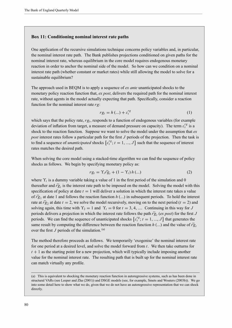
The Bank of England Quarterly Model
Box 11: Conditioning nominal interest rate paths
One application of the recursive simulations technique concerns policy variables and, in particular,the nominal interest rate path. The Bank publishes projections conditioned on given paths for thenominal interest rate, whereas equilibrium in the core model requires endogenous monetaryreaction in order to anchor the nominal side of the model. So how can we condition on a nominalinterest rate path (whether constant or market rates) while still allowing the model to solve for asustainable equilibrium?
The approach used in BEQM is to apply a sequence of ex ante unanticipated shocks to themonetary policy reaction function that, ex post, delivers the required path for the nominal interestrate, without agents in the model actually expecting that path. Specifically, consider a reactionfunction for the nominal interest rate rg:
rgt = h (...)+ εrgt (1)
which says that the policy rate, rgt , responds to a function of endogenous variables (for exampledeviation of inflation from target, a measure of demand pressure on capacity). The term εrgt is ashock to the reaction function. Suppose we want to solve the model under the assumption that expost interest rates follow a particular path for the first J periods of the projection. Then the task isto find a sequence of unanticipated shocks εrgt ; t = 1, ..., J such that the sequence of interestrates matches the desired path.
When solving the core model using a stacked-time algorithm we can find the sequence of policyshocks as follows. We begin by specifying monetary policy as:
rgt = ϒtrgt + (1−ϒt) h (...) (2)
where ϒt is a dummy variable taking a value of 1 in the first period of the simulation and 0thereafter and rgt is the interest rate path to be imposed on the model. Solving the model with thisspecification of policy at date t = 1 will deliver a solution in which the interest rate takes a valueof rg1 at date 1 and follows the reaction function h (...) in subsequent periods. To hold the interestrate at rg2 at date t = 2, we solve the model recursively, moving on to the next period (t = 2) andsolving again, this time with ϒ2 = 1 and ϒt = 0 for t = 3, 4, .... Continuing in this way for Jperiods delivers a projection in which the interest rate follows the path rgt (ex post) for the first Jperiods. We can find the sequence of unanticipated shocks εrgt ; t = 1, ..., J that generates thesame result by computing the difference between the reaction function h (...) and the value of rgtover the first J periods of the simulation. (a)
The method therefore proceeds as follows. We temporarily ‘exogenise’ the nominal interest ratefor one period at a desired level, and solve the model forward from t . We then take outturns fort + 1 as the starting point for a new projection, which will typically include imposing anothervalue for the nominal interest rate. The resulting path that is built up for the nominal interest ratecan match virtually any profile.
(a) This is equivalent to shocking the monetary reaction function in autoregressive systems, such as has been done instructural VARs (see Leeper and Zha (2001)) and DSGE models (see, for example, Smets and Wouters (2003b)). We gointo some detail here to show what we do, given that we do not have an autoregressive representation that we can shockdirectly.
80
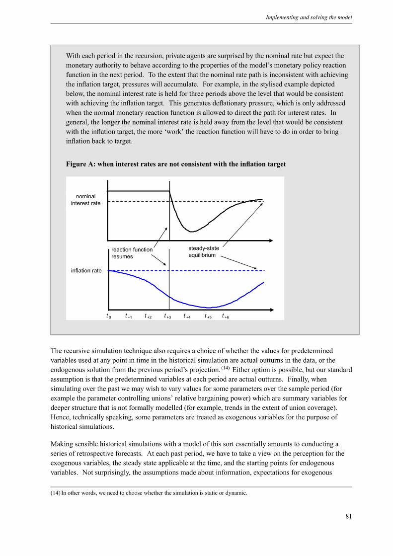
Implementing and solving the model
With each period in the recursion, private agents are surprised by the nominal rate but expect themonetary authority to behave according to the properties of the model’s monetary policy reactionfunction in the next period. To the extent that the nominal rate path is inconsistent with achievingthe inflation target, pressures will accumulate. For example, in the stylised example depictedbelow, the nominal interest rate is held for three periods above the level that would be consistentwith achieving the inflation target. This generates deflationary pressure, which is only addressedwhen the normal monetary reaction function is allowed to direct the path for interest rates. Ingeneral, the longer the nominal interest rate is held away from the level that would be consistentwith the inflation target, the more ‘work’ the reaction function will have to do in order to bringinflation back to target.
Figure A: when interest rates are not consistent with the inflation target
nominal interest rate
t 0 t +1 t +2 t +3 t +4 t +5 t +6
inflation rate
reaction function resumes
steady-stateequilibrium
The recursive simulation technique also requires a choice of whether the values for predeterminedvariables used at any point in time in the historical simulation are actual outturns in the data, or theendogenous solution from the previous period’s projection. (14) Either option is possible, but our standardassumption is that the predetermined variables at each period are actual outturns. Finally, whensimulating over the past we may wish to vary values for some parameters over the sample period (forexample the parameter controlling unions’ relative bargaining power) which are summary variables fordeeper structure that is not formally modelled (for example, trends in the extent of union coverage).Hence, technically speaking, some parameters are treated as exogenous variables for the purpose ofhistorical simulations.
Making sensible historical simulations with a model of this sort essentially amounts to conducting aseries of retrospective forecasts. At each past period, we have to take a view on the perception for theexogenous variables, the steady state applicable at the time, and the starting points for endogenousvariables. Not surprisingly, the assumptions made about information, expectations for exogenous
(14) In other words, we need to choose whether the simulation is static or dynamic.
81

The Bank of England Quarterly Model
variables, the values of predetermined variables, and the values of parameters over the past can havelarge effects on the simulated historical paths of endogenous variables.
5.4.2 Forecast projections
In a standard simulation, we would assume that the model economy was initially at equilibrium, shockthe model at time t , and solve the model to get new values for endogenous variables. But a forecast usesrecent data as the initial starting point and solves the model to see how endogenous variables would needto move over the medium term to achieve (eventually) the assumed steady-state equilibrium. The pathsfrom the model are stationary and effectively represent deviations around underlying trends for labourproductivity growth, output growth, and inflation. To derive solutions for data in levels, we scale thesesolution paths up by the appropriate growth rates, given the starting points. Effectively, the outputs fromthe full model are converted back into units that correspond to original data sources by reversing thetransformations that take place when deriving the model-consistent database – this process is explainedin detail in Section 6.2.1. We also make use of a set of transformation equations that takes some of theoutputs from the model and recombines them to construct useful diagnostic measures such as thesavings ratio.
Thus, a forecast profile is built up in the following steps:
1. Profiles for expectations of future exogenous variables are derived using the exogenous variablesmodel.
2. Values for forecast assumptions (endogenous fixes) are decided.
3. Terminal conditions for endogenous variables are calculated using the steady-state model.
4. The dynamic model is simulated recursively, taking the (possibly different) steady-state values ateach period in the projection, using the first period’s forecast values from the previous period’sprojection. A linearised model is simulated first, which the non-linear core model then uses forinitial guesses for endogenous values. The first period’s responses for each projection are extractedand form the final core model values.
5. The full model with non-core dynamics is solved, (15) given the complete path for the endogenousvalues in the core. Residual adjustments can be made to the non-core equations and the model canbe solved again.
6. The outputs from the full model, expressed in model units, are transformed into more familiarmeasures, such as National Accounts units and growth rates, for analysis.
Judgement can be added at each step: for example, if it were thought that consumption was too low overthe forecast horizon, this could reflect a number of possible issues such as the long-run equilibrium ofthe model being too low; or medium-term expectations of future labour income, price changes, taxes orreal interest rates needing modification; or the short-term forecast profile looking implausible relative toshort-term indicators. The perceived source of the problem would determine whether the forecastershould look at parameters driving the steady state, reconsider the profile for exogenous variables overthe forecast horizon, or change residual settings on the non-core model.
(15)We could in principle use the responses from the full model as the starting points for the core in the next period, but we donot do so and instead use core values as starting points for the core model going forward.
82

Implementing and solving the model
5.5 Summary
This chapter discusses how the model is set up and solved. Importantly, the model is a system ofnon-linear difference equations that contains leads as well as lags, and so requires specialised solutionalgorithms. We have also developed further routines employed in simulating the model. These are quiteelaborate, so here we summarise the key ingredients.
The model is designed to settle on a long-run sustainable equilibrium, so we have to specify thosevalues. Hence all simulations require an internally consistent steady-state solution. The core model isused to generate a steady-state model for this task that can be solved in a straightforward way.
We always need starting values for those endogenous variables that have lags. In one type of exercise –typically for demonstrating theoretical properties – we can shock the model from an initial steady-stateequilibrium, by changing the value of one or more exogenous variables. For a permanent shock, wewould need to re-solve the steady-state model to provide a new set of terminal conditions, but not for atemporary shock.
Forecasts use recent data outturns as the starting point. The model’s dynamics show how we can getfrom these starting values to the sustainable equilibrium implied by the values from the steady-statemodel. The forecast is a more complicated exercise than a simple ‘one shock’ simulation. Our standardapproach is to build up the forecast path by recursive simulations, so that we can apply judgement anddeal with issues of expectations, information sets, temporary fixes on endogenous variables.
83


Chapter 6 Parameterisation and evaluation
This chapter discusses our approach to parameterising BEQM. After a brief discussion of some initialissues (Section 6.1), Section 6.2 describes the construction of the model-consistent database. Theparameterisation of the structural core model is discussed in Section 6.3, and that of the ad hoc non-coreequations in Section 6.4. The results of a formal evaluation of the model (Section 6.5) are followed by asummary in Section 6.6.
6.1 Issues in parameterising the core model
Our basic approach has been to decide, first, which theoretical mechanisms are required for the model toserve as a useful tool for policy analysis, and then to work towards matching the data. (1) This approachputs a great deal of emphasis on viewing the model as a system. (2) It follows that because the model hasbeen built as a system, and will be operated and used as a system, it should be parameterised andevaluated as a system. However, there are several features of the model that raise difficult questions forparameterisation.
First, like many other macro models used in policy institutions, BEQM is large, simultaneous, andnon-linear. In ideal circumstances, we would estimate the model using maximum likelihood methods,which have the major benefit of consistent estimates and (asymptotic) normality. This would require usto specify correctly the stochastic structure of the model, but its non-linearity means that we would losethese desirable properties if there were any deviation from a correct specification. (3) A linearised modelwould provide some protection from the effects of misspecification. However, we cannot assume a fixedsteady-state around which to linearise the model, because the steady state itself is assumed to changeover the past, and possibly over the projection period as well.
An alternative would be to use some form of method of moments estimation, which would not require afull specification of the probability spaces (eg for parameters). But that approach is still not immune tomisspecification, and would require a large number of moment conditions in a large model such asBEQM. Aside from representing a significant computational challenge, the number of observationswould need to be much larger than the number of moment conditions. In general, ‘textbook’econometric approaches assume that there is a (very) large number of observations in the sample relativeto the number of parameters being estimated. This condition does not hold in our case. (4)
There is also a question as to how to evaluate the parameterisation of the model. As described inChapter 2, the main motivation for the new model was to improve theoretical consistency and clarity, sothat policymakers can make projections with confidence that they understand the forces generating the
(1) In terms of the modelling ‘frontier’ shown in Figure 2.1, we can think of this as moving north, then east, rather than viceversa. For simulation evidence on the merits of this strategy, see Kapetanios et al (2004).(2) This is hardly new: the Cowles Foundation approach to econometrics is famous for its concentration on the estimation oflarge, simultaneous equation models, going as far back as the Klein (1950) model.(3) And in practice we will be more concerned with the fit of the model in some dimensions than others. So it is not clear thata classical likelihood perspective is the right one, since maximum likelihood weights different moments according to theamount of information the data have about these moments. See pages 1613-14 of Eichenbaum (1995).(4) This situation is not unusual in macromodelling. Indeed, as Sims (2002, page 15) has noted: ‘Taking account ofsimultaneity ... seemed to require a lot of work to end up with results that were arbitrary (if based on a truncated instrumentlist), almost OLS (2SLS with all available instruments), or quirky (FIML and LIML).’ However, alternative approaches maybecome feasible in future.
85
The Bank of England Quarterly Model
outputs from the model and how they are affected by policy decisions. Inevitably this means that thenew model will not mechanically generate the best possible forecast, nor fit the data as well as adata-based atheoretical model. At the same time, some congruence with the data is needed to make theexercise meaningful. But the best forecasting models can be of limited use for policymakers if theycannot be used to analyse economic issues. (5) Consequently, a measure of statistical fit is not the be-alland end-all for assessing a model such as BEQM.
We do not pretend to have solved these problems. Our parameterisation strategy has been simple andpragmatic, especially for the core model. As a first pass, this has been calibrated using a range ofinformation from different sources. As explained in Section 6.3, there is a good deal of structure to thecalibration. First, we have broken the parameterisation of the model down into smaller steps, whereresults still depend on the whole system but there is a smaller set of variables to consider. For example,some variables affect only the numerical steady state, so we approach these first. Second, while themodel is highly simultaneous, there are sensible ways of ordering the use of equilibrium relations fromthe core model to estimate its underlying parameters. Third, since projections using the model are basedon model-consistent expectations, we simulate the model over history on the same basis (in effect, werun a series of recursive projections).
Advances in numerical and computational methods may make it feasible in the future to estimate thewhole model using more formal methods. In any case, the current parameterisation is not set in stone: itis frequently reappraised, and parameter values may be revisited in response to signs of structural breaksor when there are large data revisions (such as the adoption of chain linking in the National Accounts).This applies not only to the parameterisation of the model’s dynamics but also to the steady-state valuesshown in Section 6.3. Before we proceed to the choice of parameter values, however, we need toaddress a number of data issues.
6.2 The model-consistent database
The first step towards parameterising the model is to create a model-consistent database. This has twokey aspects: the data are detrended so that the model can be written in stationary form; and the data arematched to model concepts. When we refer to ‘model units’, we therefore mean data that have beendetrended and may have been modified compared with, say, a National Accounts measure, to make abetter match with the relevant economic concept.
6.2.1 Detrending and retransforming to levels
BEQM uses data that have been transformed into stationary form (as discussed in Section 5.1.3):variables are detrended by potential output growth, labour productivity growth, or inflation, asappropriate (Box 12 on page 88 sets out the process in more detail). Thus, leads and lags in the modelequations are scaled by growth rates of productive potential, productivity or inflation. A simple examplefor a real flow is the housing investment stock-flow condition:
idt = dt − 1− δdt ·dt−11+ yt
(5) The potential trade-off between theoretical consistency and data coherence is discussed in the context of Figure 2.1 inChapter 2.
86
Parameterisation and evaluation
where id is the flow of dwellings investment, d is the stock of dwellings, and y is the growth rate ofproductive potential. Where nominal scaling is involved, a detrended form requires lags to be scaleddown by growth and inflation (leads are similarly scaled up), as in the expression for seigniorage:
pct · mont − pct−1 · mont−1(1+ pt)(1+ yt)
Such detrended data must be re-transformed if data in levels are required. Examples of thesetransformations are given in Appendix C, but some general principles can be listed here.
For most real variables, such as goods and assets, the appropriate scalar is the growth rate of productivepotential, (1+ y). This is a function of the population growth rate and the labour productivity growthrate: (1+ y) = (1+ n) · 1+ λ . (6) So real variables (ie volumes) will be transformed to levels bymultiplying by the levels of both the population (N ) and labour productivity (λ). For example, thevolume of housing investment in levels (analogous to a constant price measure) will be I D = id · N · λ,where I D is a volume measure and id is in detrended model units. The notation we use to distinguishactual and detrended model units is set out in Section 6.2.2 and Table 6.1.
For variables associated with the wage schedule, the appropriate scaling is by labour productivitygrowth, (1+ λ). These variables in model units would be transformed back to levels using the level oflabour productivity. So the real private sector wage rate in levels would be given by w · λ.
As discussed in Chapter 5, prices in BEQM are relative to a numeraire price level, which we have chosen(without loss of generality) to be the consumption price level (excluding actual and imputed rents). Thenumeraire price level in the model, PC , is used to detrend other nominal prices and hence turn them intorelative prices (denoted here in lower case). By implication, the relative price of the numeraire, pc = 1in every period. Other price levels (ie deflators) are equal to the appropriate relative price multiplied bythe consumption price level (PC). For example, the nominal price of exports is PX = px · PC . (7)
Changes in the level of PC over time are given by the inflation rate, p. The numeraire price levelsimply cumulates inflation from an initial starting point, so there is a unique condition for the totalconsumption deflator: PCt = PCt−1 · (1+ pt).
Nominal variables (current price measures) simply apply both price and real levels transforms. Forexample, nominal export expenditure is PX · X = x · N · λ · px · PC , scaled back up to a nominal levelby re-introducing cumulative inflation (including the relative price, px) and growth, N · λ. The nominalwage, on the other hand, only scales by labour productivity and the price level: W = w · λ · PC .
(6) Here, we use n and λ to refer to actual growth rates of population and labour productivity. Their product y, however, is thegrowth rate of productive potential rather than actual output.(7) We calculate relative prices by dividing each price level by the consumption deflator, PC . For instance, the exampleshown in the text easily rearranges to pxt = PXt/PCt . For the consumption deflator, however, this becomespct = PCt/PCt = 1.
87
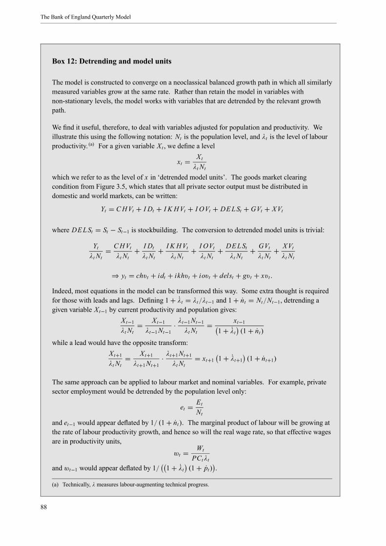
The Bank of England Quarterly Model
Box 12: Detrending and model units
The model is constructed to converge on a neoclassical balanced growth path in which all similarlymeasured variables grow at the same rate. Rather than retain the model in variables withnon-stationary levels, the model works with variables that are detrended by the relevant growthpath.
We find it useful, therefore, to deal with variables adjusted for population and productivity. Weillustrate this using the following notation: Nt is the population level, and λt is the level of labourproductivity. (a) For a given variable Xt , we define a level
xt = Xtλt Nt
which we refer to as the level of x in ‘detrended model units’. The goods market clearingcondition from Figure 3.5, which states that all private sector output must be distributed indomestic and world markets, can be written:
Yt = CHVt + I Dt + I K HVt + I OVt + DELSt + GVt + XVt
where DELSt = St − St−1 is stockbuilding. The conversion to detrended model units is trivial:Ytλt Nt
= CHVtλt Nt
+ I Dtλt Nt
+ I K HVtλt Nt
+ I OVtλt Nt
+ DELStλt Nt
+ GVtλt Nt
+ XVtλt Nt
⇒ yt = chvt + idt + ikhvt + iovt + delst + gvt + xvt .Indeed, most equations in the model can be transformed this way. Some extra thought is requiredfor those with leads and lags. Defining 1+ λt = λt/λt−1 and 1+ nt = Nt/Nt−1, detrending agiven variable Xt−1 by current productivity and population gives:
Xt−1λt Nt
= Xt−1λt−1Nt−1
· λt−1Nt−1λt Nt
= xt−11+ λt (1+ nt)
while a lead would have the opposite transform:Xt+1λt Nt
= Xt+1λt+1Nt+1
· λt+1Nt+1λt Nt
= xt+1 1+ λt+1 (1+ nt+1)
The same approach can be applied to labour market and nominal variables. For example, privatesector employment would be detrended by the population level only:
et = EtNt
and et−1 would appear deflated by 1/ (1+ nt). The marginal product of labour will be growing atthe rate of labour productivity growth, and hence so will the real wage rate, so that effective wagesare in productivity units,
wt = WtPCtλt
and wt−1 would appear deflated by 1/ 1+ λt (1+ pt) .(a) Technically, λ measures labour-augmenting technical progress.
88

Parameterisation and evaluation
Prices are expressed relative to numeraire price, which is the price of the total (non-durable)consumption bundle. For example, the relative price of export goods in the model is written aspxt = PXt/PCt . In the steady state, all price levels will increase at the rate of inflation, pss , sothe relative prices are constant:
pxt = PXtPCt
= 1+ pss
1+ pssPXt−1PCt−1
= PXt−1PCt−1
= pxt−1But if we want to deal correctly with relative prices with lags or leads, we have to be careful toaccount for inflation:
PXt−1PCt
= PXt−1PCt−1
· PCt−1PCt
= pxt−11+ pt
6.2.2 Matching model concepts
The model has been designed to observe a number of consistency conditions, especially stock-flow andflow-flow conditions (such as budget constraints), as discussed in Section 4.2.2. These consistencyconditions may not always be observed in the raw data, especially if different components come frominconsistent sources. But the model’s theory does not recognise the differences between, say, NationalAccounts and public finances definitions of government spending. So we need to adjust the data tosatisfy these conditions.
In addition, official measures may be only approximate matches to underlying economic concepts. Thecomponents of particular expenditures, taxes and transfers need to be aligned as closely as possible withthe underlying decision-making structure of the core theory. This may imply disaggregating andreaggregating in different ways (Box 3 on page 36 discusses the treatment of government and privatesector output). However, there are some cases where data that have no obvious model counterpart haveto be aggregated into other model variables to account for all flows and stocks.
This section illustrates how the main model concepts map into the National Accounts and other datasources; more detailed data sources are listed in Appendix C. For simplicity in this section, we do notadd time subscripts if a data relationship is contemporaneous. They are included where necessary (suchas stock-flow relationships), but we abstract from the scaling that would be implied by the detrendingprocedures described in Section 6.2.1.
Nominal spending, volumes, prices and the National Accounts
The key measure of activity in BEQM is private sector output. But there is a straightforward mappingbetween this and GDP as measured in the National Accounts. As far as possible we apply a consistentmapping between model concepts and National Accounts data. Nominal expenditures on different typesof goods in the model are linked to the corresponding National Accounts measures. Similarly, thevolume of different types of goods and services produced by firms in the model are linked to theequivalent to the National Accounts chained volume measure; and the prices of different goods andservices in BEQM are equivalent to the corresponding National Accounts price deflators.
We adopt a particular naming convention for National Accounts data in the model: a ‘cp’ suffix istypically used to denote National Accounts data for nominal expenditure (current prices); a ‘kp’ suffix isused for the corresponding chained volume measure (expressed in terms of the current reference year’sprices); and a ‘def ’ suffix is used to denote the implicit expenditure deflator; detrended model units are
89
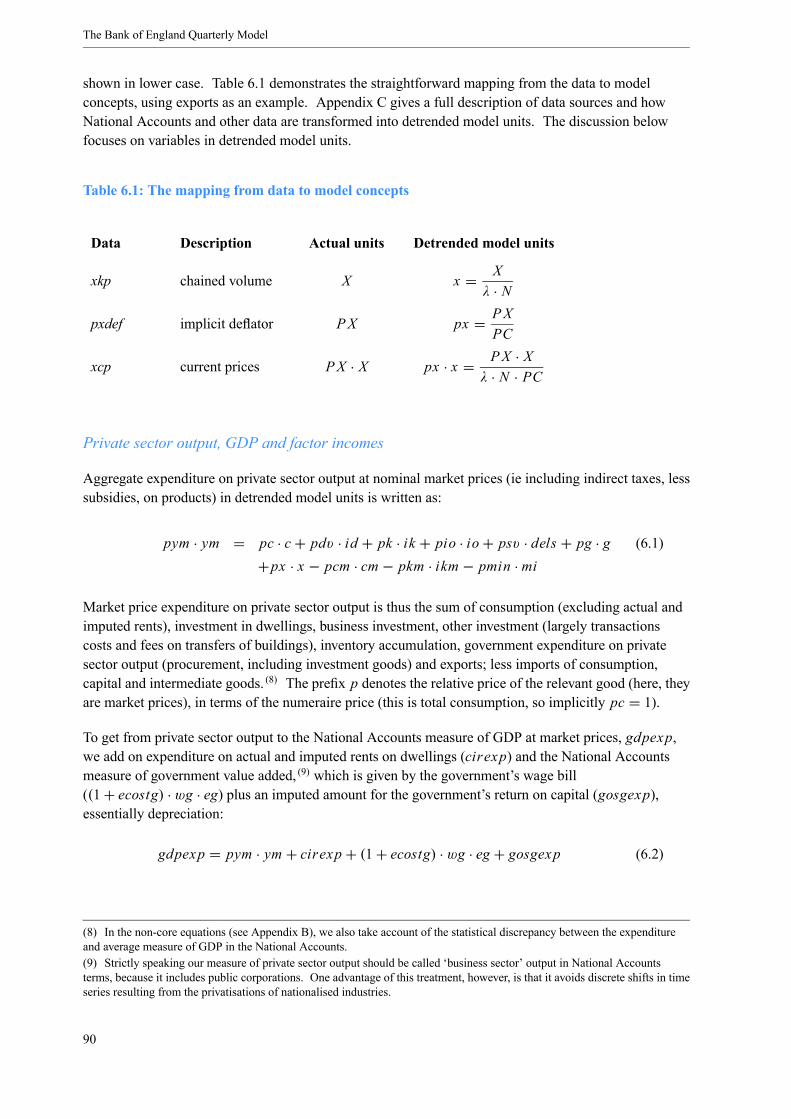
The Bank of England Quarterly Model
shown in lower case. Table 6.1 demonstrates the straightforward mapping from the data to modelconcepts, using exports as an example. Appendix C gives a full description of data sources and howNational Accounts and other data are transformed into detrended model units. The discussion belowfocuses on variables in detrended model units.
Table 6.1: The mapping from data to model concepts
Data Description Actual units Detrended model units
xkp chained volume X x = Xλ · N
pxdef implicit deflator PX px = PXPC
xcp current prices PX · X px · x = PX · Xλ · N · PC
Private sector output, GDP and factor incomes
Aggregate expenditure on private sector output at nominal market prices (ie including indirect taxes, lesssubsidies, on products) in detrended model units is written as:
pym · ym = pc · c + pdv · id + pk · ik + pio · io+ psv · dels + pg · g (6.1)+px · x − pcm · cm − pkm · ikm − pmin · mi
Market price expenditure on private sector output is thus the sum of consumption (excluding actual andimputed rents), investment in dwellings, business investment, other investment (largely transactionscosts and fees on transfers of buildings), inventory accumulation, government expenditure on privatesector output (procurement, including investment goods) and exports; less imports of consumption,capital and intermediate goods. (8) The prefix p denotes the relative price of the relevant good (here, theyare market prices), in terms of the numeraire price (this is total consumption, so implicitly pc = 1).
To get from private sector output to the National Accounts measure of GDP at market prices, gdpexp,we add on expenditure on actual and imputed rents on dwellings (cirexp) and the National Accountsmeasure of government value added, (9) which is given by the government’s wage bill((1+ ecostg) · wg · eg) plus an imputed amount for the government’s return on capital (gosgexp),essentially depreciation:
gdpexp = pym · ym + cirexp + (1+ ecostg) · wg · eg + gosgexp (6.2)
(8) In the non-core equations (see Appendix B), we also take account of the statistical discrepancy between the expenditureand average measure of GDP in the National Accounts.(9) Strictly speaking our measure of private sector output should be called ‘business sector’ output in National Accountsterms, because it includes public corporations. One advantage of this treatment, however, is that it avoids discrete shifts in timeseries resulting from the privatisations of nationalised industries.
90
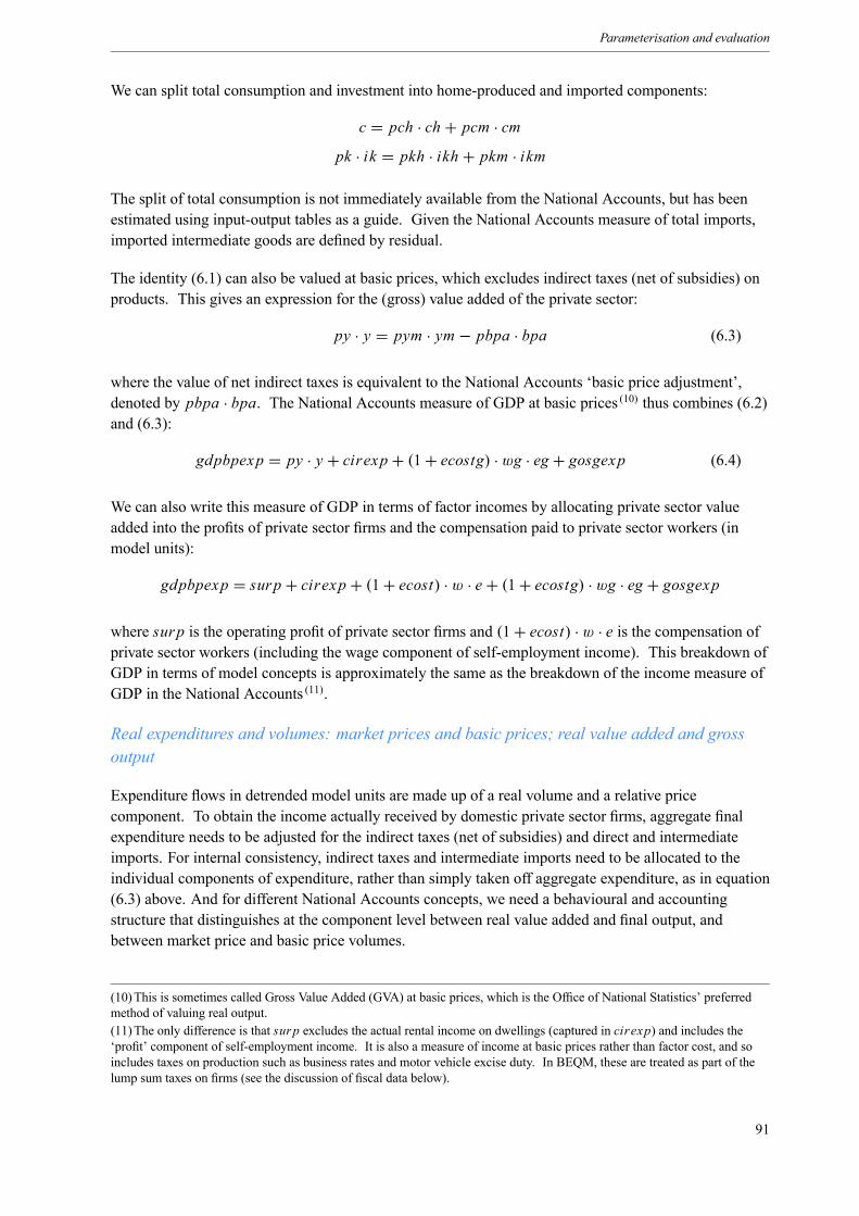
Parameterisation and evaluation
We can split total consumption and investment into home-produced and imported components:
c = pch · ch + pcm · cmpk · ik = pkh · ikh + pkm · ikm
The split of total consumption is not immediately available from the National Accounts, but has beenestimated using input-output tables as a guide. Given the National Accounts measure of total imports,imported intermediate goods are defined by residual.
The identity (6.1) can also be valued at basic prices, which excludes indirect taxes (net of subsidies) onproducts. This gives an expression for the (gross) value added of the private sector:
py · y = pym · ym − pbpa · bpa (6.3)
where the value of net indirect taxes is equivalent to the National Accounts ‘basic price adjustment’,denoted by pbpa · bpa. The National Accounts measure of GDP at basic prices (10) thus combines (6.2)and (6.3):
gdpbpexp = py · y + cirexp + (1+ ecostg) ·wg · eg + gosgexp (6.4)
We can also write this measure of GDP in terms of factor incomes by allocating private sector valueadded into the profits of private sector firms and the compensation paid to private sector workers (inmodel units):
gdpbpexp = surp + cirexp + (1+ ecost) · w · e+ (1+ ecostg) · wg · eg + gosgexp
where surp is the operating profit of private sector firms and (1+ ecost) · w · e is the compensation ofprivate sector workers (including the wage component of self-employment income). This breakdown ofGDP in terms of model concepts is approximately the same as the breakdown of the income measure ofGDP in the National Accounts (11).
Real expenditures and volumes: market prices and basic prices; real value added and grossoutput
Expenditure flows in detrended model units are made up of a real volume and a relative pricecomponent. To obtain the income actually received by domestic private sector firms, aggregate finalexpenditure needs to be adjusted for the indirect taxes (net of subsidies) and direct and intermediateimports. For internal consistency, indirect taxes and intermediate imports need to be allocated to theindividual components of expenditure, rather than simply taken off aggregate expenditure, as in equation(6.3) above. And for different National Accounts concepts, we need a behavioural and accountingstructure that distinguishes at the component level between real value added and final output, andbetween market price and basic price volumes.
(10)This is sometimes called Gross Value Added (GVA) at basic prices, which is the Office of National Statistics’ preferredmethod of valuing real output.(11)The only difference is that surp excludes the actual rental income on dwellings (captured in cirexp) and includes the‘profit’ component of self-employment income. It is also a measure of income at basic prices rather than factor cost, and soincludes taxes on production such as business rates and motor vehicle excise duty. In BEQM, these are treated as part of thelump sum taxes on firms (see the discussion of fiscal data below).
91
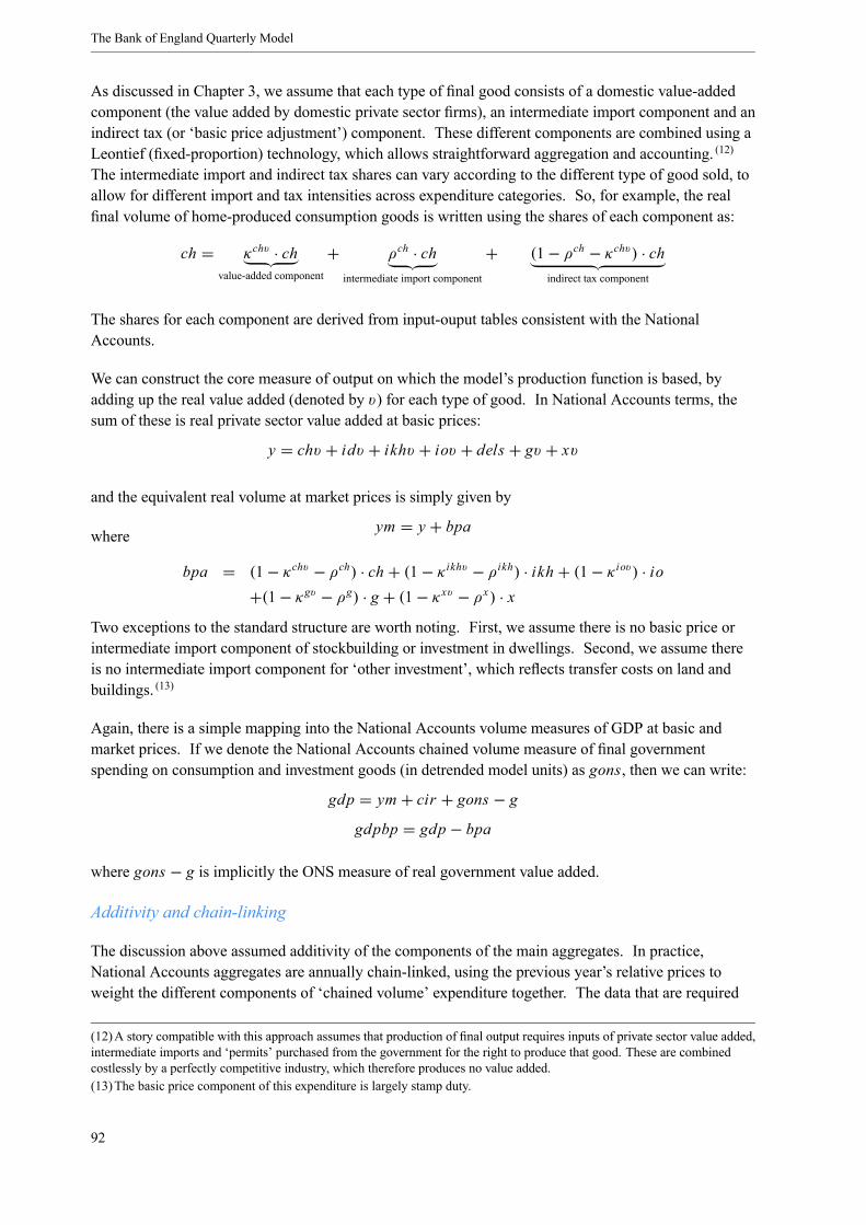
The Bank of England Quarterly Model
As discussed in Chapter 3, we assume that each type of final good consists of a domestic value-addedcomponent (the value added by domestic private sector firms), an intermediate import component and anindirect tax (or ‘basic price adjustment’) component. These different components are combined using aLeontief (fixed-proportion) technology, which allows straightforward aggregation and accounting. (12)
The intermediate import and indirect tax shares can vary according to the different type of good sold, toallow for different import and tax intensities across expenditure categories. So, for example, the realfinal volume of home-produced consumption goods is written using the shares of each component as:
ch = κchv · chvalue-added component
+ ρch · chintermediate import component
+ (1− ρch − κchv ) · chindirect tax component
The shares for each component are derived from input-ouput tables consistent with the NationalAccounts.
We can construct the core measure of output on which the model’s production function is based, byadding up the real value added (denoted by v) for each type of good. In National Accounts terms, thesum of these is real private sector value added at basic prices:
y = chv + idv + ikhv + iov + dels + gv + xv
and the equivalent real volume at market prices is simply given by
ym = y + bpawhere
bpa = (1− κchv − ρch) · ch + (1− κ ikhv − ρikh) · ikh + (1− κ iov ) · io+(1− κgv − ρg) · g + (1− κ xv − ρx) · x
Two exceptions to the standard structure are worth noting. First, we assume there is no basic price orintermediate import component of stockbuilding or investment in dwellings. Second, we assume thereis no intermediate import component for ‘other investment’, which reflects transfer costs on land andbuildings. (13)
Again, there is a simple mapping into the National Accounts volume measures of GDP at basic andmarket prices. If we denote the National Accounts chained volume measure of final governmentspending on consumption and investment goods (in detrended model units) as gons, then we can write:
gdp = ym + cir + gons − ggdpbp = gdp − bpa
where gons − g is implicitly the ONS measure of real government value added.
Additivity and chain-linking
The discussion above assumed additivity of the components of the main aggregates. In practice,National Accounts aggregates are annually chain-linked, using the previous year’s relative prices toweight the different components of ‘chained volume’ expenditure together. The data that are required
(12)A story compatible with this approach assumes that production of final output requires inputs of private sector value added,intermediate imports and ‘permits’ purchased from the government for the right to produce that good. These are combinedcostlessly by a perfectly competitive industry, which therefore produces no value added.(13)The basic price component of this expenditure is largely stamp duty.
92
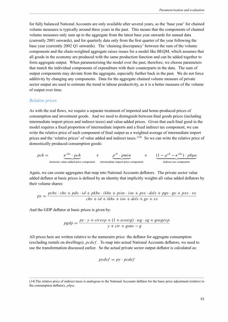
Parameterisation and evaluation
for fully balanced National Accounts are only available after several years, so the ‘base year’ for chainedvolume measures is typically around three years in the past. This means that the components of chainedvolume measures only sum up to the aggregate from the latest base year onwards for annual data(currently 2001 onwards), and for quarterly data only from the first quarter of the year following thebase year (currently 2002 Q1 onwards). The ‘chaining discrepancy’ between the sum of the volumecomponents and the chain-weighted aggregate raises issues for a model like BEQM, which assumes thatall goods in the economy are produced with the same production function and can be added together toform aggregate output. When parameterising the model over the past, therefore, we choose parametersthat match the individual components of expenditure with their counterparts in the data. The sum ofoutput components may deviate from the aggregate, especially further back in the past. We do not forceadditivity by changing any components. Data for the aggregate chained volume measure of privatesector output are used to estimate the trend in labour productivity, as it is a better measure of the volumeof output over time.
Relative prices
As with the real flows, we require a separate treatment of imported and home-produced prices ofconsumption and investment goods. And we need to distinguish between final goods prices (includingintermediate import prices and indirect taxes) and value-added prices. Given that each final good in themodel requires a fixed proportion of intermediate imports and a fixed indirect tax component, we canwrite the relative price of each component of final output as a weighted average of intermediate importprices and the ‘relative prices’ of value added and indirect taxes. (14) So we can write the relative price ofdomestically produced consumption goods:
pch = κchv · pchdomestic value-added price component
+ ρch · pminintermediate import price component
+ (1− ρch − κchv ) · pbpaindirect tax component
Again, we can create aggregates that map into National Accounts deflators. The private sector valueadded deflator at basic prices is defined by an identity that implicitly weights all value added deflators bytheir volume shares:
py = pchv · chv + pdv · id + pkhv · ikhv + piov · iov + psv · dels + pgv · gv + pxv · xvchv + id + ikhv + iov + dels + gv + xv
And the GDP deflator at basic prices is given by:
pgdp = py · y + cirexp + (1+ ecostg) · wg · eg + gosgexpy + cir + gons − g
All prices here are written relative to the numeraire price: the deflator for aggregate consumption(excluding rentals on dwellings), pcde f . To map into actual National Accounts deflators, we need touse the transformation discussed earlier. So the actual private sector output deflator is calculated as:
pyde f = py · pcde f
(14)The relative price of indirect taxes is analogous to the National Accounts deflator for the basic price adjustment (relative tothe consumption deflator), pbpa.
93
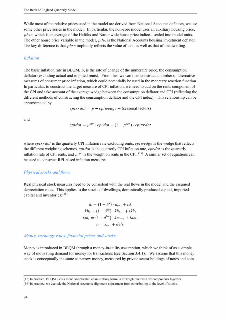
The Bank of England Quarterly Model
While most of the relative prices used in the model are derived from National Accounts deflators, we usesome other price series in the model. In particular, the non-core model uses an auxiliary housing price,phse, which is an average of the Halifax and Nationwide house price indices, scaled into model units.The other house price variable in the model, pdv , is the National Accounts housing investment deflator.The key difference is that phse implicitly reflects the value of land as well as that of the dwelling.
Inflation
The basic inflation rate in BEQM, p, is the rate of change of the numeraire price, the consumptiondeflator (excluding actual and imputed rents). From this, we can then construct a number of alternativemeasures of consumer price inflation, which could potentially be used in the monetary reaction function.In particular, to construct the target measure of CPI inflation, we need to add on the rents component ofthe CPI and take account of the average wedge between the consumption deflator and CPI (reflecting thedifferent methods of constructing the consumption deflator and the CPI index). This relationship can beapproximated by
cpixrdot = p − cpiwedge+ (seasonal factors)
andcpidot = µcpr · cprdot + (1− µcpr ) · cpixrdot
where cpixrdot is the quarterly CPI inflation rate excluding rents, cpiwedge is the wedge that reflectsthe different weighting schemes, cpidot is the quarterly CPI inflation rate, cprdot is the quarterlyinflation rate of CPI rents, and µcpr is the weight on rents in the CPI. (15) A similar set of equations canbe used to construct RPI-based inflation measures.
Physical stocks and flows
Real physical stock measures need to be consistent with the real flows in the model and the assumeddepreciation rates. This applies to the stocks of dwellings, domestically produced capital, importedcapital and inventories: (16)
dt = 1− δd · dt−1 + idtkht = 1− δkh · kht−1 + ikhtkmt = 1− δkm · kmt−1 + ikmt
st = st−1 + delst
Money, exchange rates, financial prices and stocks
Money is introduced in BEQM through a money-in-utility assumption, which we think of as a simpleway of motivating demand for money for transactions (see Section 3.4.1). We assume that this moneystock is conceptually the same as narrow money, measured by private sector holdings of notes and coin.
(15) In practice, BEQM uses a more complicated chain-linking formula to weight the two CPI components together.(16) In practice, we exclude the National Accounts alignment adjustment from contributing to the level of stocks.
94

Parameterisation and evaluation
Real exchange rate measures take the exchange rate index (ERI) (17) and adjust for relative domestic andoverseas consumer price levels.
We have a variety of financial assets in the model. They must satisfy the model identities
a = v + bk + pg · bg + pc · mon + nfanfa = bf /q
such that real household financial asset holdings are equal to the sum of the real values of equities,corporate bonds, government bonds, money and net foreign assets.
Financial intermediaries are not modelled explicitly in BEQM, so households are assumed to holdfinancial assets directly, including those which in practice are held on their behalf by pension funds andother financial companies. We also use a narrow definition of money, so households’ holdings ofdeposits with monetary financial institutions and household sector debt are not separately identified.
Implicitly, the stock of households’ deposit holdings (net of their secured and unsecured debt) is treatedas part of households’ net equity holdings, even though deposit and debt instruments may in practiceprovide specialist services (for example, bank deposits providing transactions services). This means thatthe conceptual definitions of different assets in the model only correspond to the balance sheet datafound in the National Accounts at a highly aggregated level. (18)
Asset stocks are measured at market values. So the accumulation identities in the model need to takeaccount of changes in the market values of different asset stocks, such as the effect of exchange ratemovements on the domestic currency value of net foreign assets.
Savings flows in the model are assumed, where possible, to be equivalent to the concept of net lending inthe National Accounts, so the financial surplus measure used in the government budget constraint isequivalent to the National Accounts measure of general government net lending; and the overseas sectorflow equates to the current account of the balance payments plus net capital transfers. (19)
The assumption of a small set of one-period, risk-free assets pinned down by arbitrage relationships,means that mapping the model’s revaluation of financial assets onto those observed in the data is notstraightforward. If asset price revaluations have moved significantly differently from the arbitragerelationships in the model, we may not be able to match market values of the stocks as well as we canthe associated flows.
(17)The version of BEQM described here was calibrated on the definition of the ERI current in 2004, not the new indexproposed in Lynch and Whitaker (2004).(18)We have matched a conceptually to net financial wealth of the household sector (as defined in the National Accounts).The variable bk is a measure of Private Non-Financial Companies’ debt net of short-term liquid financial assets (constructedfrom National Accounts components); pg · bg is general government gross debt (from the National Accounts); mon is narrowmoney holdings (as defined above); and nfa is net foreign assets (as defined in the National Accounts). We define v residuallyas an implicit measure of the value of UK equities, although, as noted above, in practice this measure will contain other assetsas well.(19)Although the private sector financial deficit in the model maps into the National Accounts measure of net lending, thebreakdown into household sector and coporate sector savings flows does not correspond exactly to the net lending data in theNational Accounts. This is partly because we do not model financial intermediaries, and partly due to the treatment ofself-employment income and rents, which affects the split between profits and labour income. But the household sector savingratio and other National Accounts variables, such as the corporate profit share, are straightforward to construct from modelconcepts using some auxiliary equations.
95

The Bank of England Quarterly Model
Fiscal data
The model’s theory makes no distinction between government expenditures recorded in the NationalAccounts and those in the public finance accounts, and the two are not consistent. Our priority is forflows that are consistent with the National Accounts measure of nominal government spending, becausewe use the National Accounts framework. Government revenues and expenditures have to be capturedby the budget constraint:
(new debt)+ (seigniorage revenue)+ (tax revenue)= (transfer payments)+ (procurement of private sector goods and services)
+ (government spending on factor inputs)+ (debt servicing)
Total tax revenue is accounted for by various revenue streams as follows:
tax = taxw + taxee + taxd + taxef + taxk+taxlumpc + taxlumpk + taxf + taxind + gosgexp
Total tax receipts comprise: taxes from labour income; employees’ National Insurance Contributions;taxes on dwellings; employers’ National Insurance Contributions; corporation tax; lump-sum taxes onhouseholds and firms; tax receipts from overseas residents; and indirect taxes. The imputed return ongovernment capital (depreciation), gosgexp, is also added to match the National Accounts measure ofreceipts. Tax rates are calculated as effective rates, by dividing the revenue by the appropriate incomeflow; see the equation listing in Appendix A for details.
Transfer payments are also broken up in spending categories:
trans = transc + transu + transk + transf + transksubs + rgprem
Total transfer payments include transfers to consumers, the unemployed, firms and overseas residents;product subsidies to firms; and a ‘wedge’ on interest rates applying to government bonds. Transferrates, as with tax rates, are calculated as effective rates relative to the underlying flow.
Labour market
The labour market requires data for wages, employment, unemployment and labour supply. Laboursupply, employment and unemployment are defined in terms of Labour Force Survey (LFS) aggregates,as is the split between government and private sector employment, (20) and also private sector and wholeeconomy average hours worked. Similar to our treatment of National Accounts data, we adopt aparticular naming convention to identify LFS quantities in heads and hours in the model: the suffix hdsis denotes heads-based LFS quantities (in thousands) and hrs denotes weekly hours. Average hours areindexed in the model to take the value of 1 in 1995, this index is denoted by avh.
For transforming into detrended model units, we use the LFS measure of population aged 16+ (nhds) toequate with the model population concept, N , as discussed in Section 6.2.1. Table 6.2 illustrates this:essentially the detrending process for labour market data converts quantities in terms of heads into ratesof the population aged 16+.
(20)Private sector employment includes both employees and the self-employed, while all government sector workers aretreated as employees.
96
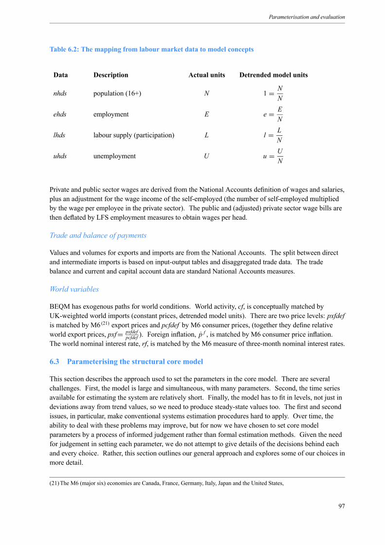
Parameterisation and evaluation
Table 6.2: The mapping from labour market data to model concepts
Data Description Actual units Detrended model units
nhds population (16+) N 1 = NN
ehds employment E e = EN
lhds labour supply (participation) L l = LN
uhds unemployment U u = UN
Private and public sector wages are derived from the National Accounts definition of wages and salaries,plus an adjustment for the wage income of the self-employed (the number of self-employed multipliedby the wage per employee in the private sector). The public and (adjusted) private sector wage bills arethen deflated by LFS employment measures to obtain wages per head.
Trade and balance of payments
Values and volumes for exports and imports are from the National Accounts. The split between directand intermediate imports is based on input-output tables and disaggregated trade data. The tradebalance and current and capital account data are standard National Accounts measures.
World variables
BEQM has exogenous paths for world conditions. World activity, cf, is conceptually matched byUK-weighted world imports (constant prices, detrended model units). There are two price levels: pxfdefis matched by M6(21) export prices and pcfdef by M6 consumer prices, (together they define relativeworld export prices, pxf= pxfdef
pcfdef ). Foreign inflation, pf , is matched by M6 consumer price inflation.
The world nominal interest rate, rf, is matched by the M6 measure of three-month nominal interest rates.
6.3 Parameterising the structural core model
This section describes the approach used to set the parameters in the core model. There are severalchallenges. First, the model is large and simultaneous, with many parameters. Second, the time seriesavailable for estimating the system are relatively short. Finally, the model has to fit in levels, not just indeviations away from trend values, so we need to produce steady-state values too. The first and secondissues, in particular, make conventional systems estimation procedures hard to apply. Over time, theability to deal with these problems may improve, but for now we have chosen to set core modelparameters by a process of informed judgement rather than formal estimation methods. Given the needfor judgement in setting each parameter, we do not attempt to give details of the decisions behind eachand every choice. Rather, this section outlines our general approach and explores some of our choices inmore detail.
(21)The M6 (major six) economies are Canada, France, Germany, Italy, Japan and the United States,
97
The Bank of England Quarterly Model
6.3.1 General approach
We can address some of the problems noted above by splitting the parameters in the core model intothree groups: those that affect only the steady state; those that affect only the dynamics; and those thataffect both the steady state and the dynamics. This allows us to divide the parameterisation process intotwo broad steps. First we choose parameters that affect only the steady state of the model, aiming tomatch broad trends in the levels of the data. Second, we choose the parameters that affect the dynamicsof the model. Because some of these parameters will also affect the steady state, some iteration betweenthe two steps will generally be required.
We do not assume that the parameters of the core model are constant over time, because we do not viewthe core model as a literal description of behaviour defined by fixed underlying parameters. This isbecause the core model is intended to provide a coherent model of decision making for differenteconomic agents, but to do this in a tractable way means that some important mechanisms cannot beincorporated into the core model and are instead proxied by parameters in the model. To the extent thatwe believe that such effects have changed over time, we allow the core model parameters to vary overthe past.
An example is the way in which the core model accounts for changes in relative (value-added) prices,given the assumption that goods are produced by a single production function. We know that there havebeen significant trends in the relative prices of expenditure components (as measured by NationalAccounts deflators) over our data sample. But aside from imported intermediates prices and taxation,the only way the core model allows for relative price movements is through different demand elasticities(and hence mark-ups) across expenditure components. So we use assumptions about demand elasticitiesthat allow us to proxy trends in relative prices. (22) Thus, we are not simply choosing a fixed number foreach parameter in the model, but in some cases a time profile over the past. (23)
6.3.2 Parameterising the steady state
Our first step is to parameterise the steady state of the model, (24) which forms the base for simulationsand the long run for forecasts. We do not think it always sensible to aim to match sample averages (ashas often been used in the DSGE literature), because some steady-state ratios show apparent regimeshifts (eg the inventory-output ratio) or persistent trends (eg the relative price of investment goods). Insuch cases, a value that differs from the historic sample average would seem more plausible for thefuture long run.
Our method was to make initial assumptions for parameter values and solve the steady-state model. (25)
Because it is stationary, the model defines the steady state as a set of numbers, such as ratios to outputand relative prices, so that evaluating the steady state against historical data is straightforward. Iterationfollows to adjust structural parameters, so that the steady state tells a coherent story relative to these data.While this process is judgemental, it is not unconstrained. First, there are more steady-state values to
(22)We recognise that this is not perfect, as some of the observed relative price trend is likely to be due to relative productivitymovements. A more fully articulated multisector model might be able to pick up some of these movements by modellingdifferential productivity trends in different sectors (this is not a trivial task, however, as data for multisectoral splits are oftenunavailable).(23)This procedure is very close, albeit informally, to estimating time series processes for parameters; see, for example, Smetsand Wouters (2003a) and Adolfson et al (2004a).(24) In common with most of the DSGE literature, we are dealing with a deterministic steady state: that is, we assume certaintyequivalence when solving the model.(25)See Chapter 5 for a discussion of how we solve the steady-state model.
98
Parameterisation and evaluation
match than there are free parameters. And, second, those free parameters affect the different steady-statevalues simultaneously. So parameters cannot be assigned to fit each steady-state property independently.In this way, the exercise of jointly fitting many steady-state values with a smaller set of parameters in atheory-consistent framework imposes a meaningful discipline on our calibration of the model.
Exogenous variables
Before choosing the parameters that determine the steady state of the model, we decompose historicalmovements in exogenous variables into transitory and permanent components. The steady state of thecore model at any moment in time depends on the expected long-run values of exogenous variables,rather than their current values, so movements in the steady state could in part reflect changingperceptions of the long-run values of exogenous variables.
We have three main types of exogenous variables:
1. domestic trend growth assumptions;
2. domestic policy targets or assumptions; and
3. assumptions for the rest of the world.
Permanent and transitory components were initially identified by applying low-frequency filters to thedata for exogenous variables. But in some cases, we adopted an alternative approach. For example,over the period of inflation targeting in the United Kingdom we set the steady-state inflation rate equal tothe announced target. (26) But there was no explicit inflation target for the early part of the sampleperiod. We could in principle apply filtering techniques to the data over that period. But instead, wederived an implicit inflation target from announced policy objectives. (27)
Parameter values
In many small models with microfoundations, a unique recursive ordering for parameters can be derivedand used to estimate the parameters. For example, calibration of the canonical Ramsey model(discussed in Box 9 on page 64) typically starts by setting the discount factor of consumers in the model,based on observations of (or assumptions about) long-run real interest rates. Then the productionfunction parameters can be chosen to match the observed capital-output ratio, and the depreciation rateto match the investment-output ratio. This process is recursive: it starts with an assumption about thediscount factor and moves on to other parameters in the model. Unfortunately, such an approach cannotbe applied directly to the core model, since the interactions in the model give rise to a greater degree ofsimultaneity and complexity – for example, changes in the real exchange rate have implications forsupply, which creates a link between the level of potential output and parameters that primarily affectdemand.
However, we can work out an approximately recursive approach that exploits the way the model is usedin practice. Some parameters in the core model can be chosen recursively, conditional on assumptionsabout certain endogenous variables. Given these judgements, we can calibrate separate parts of themodel as (relatively) self-contained blocks. The aim is to chose assumptions about endogenousvariables such that subsequent parameter settings are not inconsistent with these assumptions. To the
(26)Or the mid-point of the range, which is a straightforward assumption for a model such as this.(27) In particular, we followed closely the approach of Batini and Nelson (2000). For example, in periods of money growthtargeting, it is possible to infer an inflation target by adjusting for (published) forecasts of velocity and trend growth.
99

The Bank of England Quarterly Model
extent that these inconsistencies arise, the process can be repeated, with updated assumptions for thesteady-state endogenous variables. (28)
Key policy judgements and supply-side conditions
We begin by making judgements about the parameters that affect the historical paths of the steady-statereal exchange rate, unemployment rate and participation rate. We choose parameters that deliver aparticular steady-state path: for example, the real exchange rate profile depends on a scalar, κ x , in theexport demand function. (29) The consistency of the implicit assumptions about κ x required to supportour initial judgement can be validated at a later stage (for example, by comparison with the results ofdirect estimation of an export demand relationship and other estimates of steady state exchange rates).Assumptions about all such parameters combine to give us the steady-state exchange rate. We canvalidate the choices for such parameters and the steady states jointly by reference to other studies and toour priors.
The next step is to make a judgement about the permanent components of (both domestic and imported)relative prices in the data. These assumptions pin down important supply-side quantities, to allow us toapply a recursive approach conditional on key assumptions. For example, given the data for expendituredeflators, we make a judgement about the extent to which changes in the data were perceived astemporary or permanent. (30) The perceived permanent components are treated as the historical path forthe steady-state relative prices. For domestic prices, we choose the appropriate profile for demandelasticities across expenditure components; for import prices we choose (exogenous) paths for variablesrepresenting the relative world prices of different types of goods (intermediates, investment goods andconsumption goods). (31)
With assumptions about steady-state relative prices in place, it becomes possible to set parameters forparticular parts of the model in a more or less recursive manner. For example, the cost of capital ispinned down by assumptions about steady-state relative prices, depreciation rates of home and importedcapital and the steady-state world real interest rate. Maintaining these assumptions (by changing therelevant parameters if necessary) means that we can temporarily suppress ‘second round’ demand effectsthat would otherwise occur. This allows us to proceed with parameterisation of the supply side.
The production function
On the supply side we can estimate the production function parameters simultaneously with the level oflabour productivity, given a judgement on the path of the steady-state capital stock. (32) The iterativeestimation process starts with an initial assumption about the parameters, which is used to estimate thecoefficients of a log-linear time trend for labour productivity. Given data for private sector output and
(28)This approach could also be used for formal econometric estimation: individual equilibrium conditions or systems ofequilibrium conditions could be used to identify values for underlying parameters. However, apart from supply-sideparameters, experiments with this approach were not very successful, especially for the key household preference parameters.This is well known: see Attanasio (1999) for a critique of estimating equations using aggregate data.(29)This scalar is included because the underlying foreign demand data are measured as an index number and so do notcorrespond to the units in which domestic volumes are measured.(30)There are clearly judgements to be made about the extent to which agents may have anticipated or extrapolated apparentrelative price trends. A first step is usually to apply a simple filter to the data.(31)Data series at this level of disaggregation are not generally available, so we include parameters to allow judgementregarding relative world price movements to be applied.(32)Specifically, we estimate the production function parameters α, φ (the return-to-capital parameters in the CES productionfunction) and σ y (the elasticity of substitution between capital and labour) jointly with a log-linear time trend for labourproductivity.
100
Parameterisation and evaluation
the capital stock, and our assumptions about the path of steady-state employment and average hours, weuse the production function to estimate labour productivity using non-linear least squares. The resultingcoefficients determine both the level of labour productivity and its steady-state growth rate. Thesteady-state productivity growth rate (λss) affects decision making in the core model (throughgrowth-adjusted rates of return) and the steady state of the model is now solved and the implied path ofthe steady-state capital stock compared to the assumed path. (33) The production function parameters arethen adjusted and the estimation process repeated until the steady-state capital stock matches theassumed path as closely as possible. (34)
Preference shares
We can also exploit the use of constant elasticity of substitution functions to capture preferences (forexample, preferences between non-durable consumption and dwellings, between home and importedconsumption, and between home and imported capital). These functions imply that relative demands aresolely determined by relative prices and the parameters of the aggregator function. Given assumptionsabout relative price trends, the coefficients of these functions can be estimated using single equationtechniques. This provides initial information on how to set elasticities of substitution and shareparameters.
For example, the CES aggregator defining the preferences between home and imported consumptiongoods implies that the relative demands for these goods satisfy the simple relationship:
chtcmt
= 1− φmφm
σm−1 ψm pcht(1− ψm) pcmt
−σm
where φm and ψm are share parameters and σm is the elasticity of substitution. Taking logs allows us toestimate the regression
log cht − log cmt = A − σm log pcht − log pcmtusing ordinary least squares. This gives us a direct estimate of the substitution elasticity and theestimate of A (which is a function of φm and ψm) guides the choice of share parameters. In practice, theleft-hand and right-hand side series can take various forms. We could take the actual data forexpenditures and relative prices or the assumptions about the steady state components, or a combinationof both. Different series give different parameter estimates and this range can be used as a guide to theinitial parameter settings.
Household preference parameters
Holding the supply side fixed now, we can establish a link between demand and asset accumulation.This highlights the implications for steady-state asset positions of different values of the householdpreference parameters. A useful starting point is the marginal propensity to consume. To illustrate therole of the key parameters, if we were to simplify the model so that there were no dwellings, money, orhabits, we would have a steady-state marginal propensity to consume out of wealth given by
mpc = 1− γβσ c (1+ r)σ c−1 (6.5)
where γ is the probability of survival, β is the household discount factor, σ c is the elasticity ofintertemporal substitution in consumption, and r is the real interest rate. Equation (6.5) implies thatincreasing β reduces the marginal propensity to consume out of wealth as households become more
(33)This solution adjusts the necessary parameters to deliver the judgements on steady-state relative prices mentioned earlier.(34)Given the small number of parameters, this process was efficiently implemented using a Nelder-Mead algorithm, based onthe description in Lagarias et al (1998).
101
The Bank of England Quarterly Model
‘patient’ and forego current consumption to raise future consumption Raising γ also reduces themarginal propensity to consume – if households expect to live longer, they are more inclined to save.The effect of increasing σ c on the marginal propensity to consume depends on whether β (1+ r) isgreater or less than 1. And the effect on the marginal propensity to consume of an increase in thesteady-state real interest rate depends on the elasticity of intertemporal substitution. (35)
Steady-state consumption is equal to the (steady-state) marginal propensity to consume multiplied by(steady-state) wealth. However, the effects of parameter changes on the marginal propensity to consumedo not necessarily reflect the effects on consumption because wealth is endogenous. (36) This highlightsa key simultaneity when thinking about the effects of changes in household parameters (β, γ , σ c) onconsumption: these parameters affect both the marginal propensity to consume out of wealth and thelevel of wealth itself.
As we are holding household income and the supply of domestic assets fixed, we can now see theimplications for the economy’s net financial position. The net foreign asset position is determined bythe difference between the demand for financial assets and the supply of domestic assets (equities,corporate bonds, and government debt). (37)
nfay= desired savings − domestic assets
yGiven the supply side and the real exchange rate judgements described above, the demand sideassumptions uniquely pin down the net foreign asset position. The accumulation identity for net foreignassets is nfat = (1+ rt−1) ·nfat−1 + xt −mt+ (net transfers), where r is the world real interest rate andx −m is the trade balance. This shows that the sustainable trade balance is simply given by:
nfa = m − x − (net transfers)r
so that a negative net foreign asset position is sustainable with a positive current account flow – theeconomy has to maintain a positive trade balance in order to service debt owed to the rest of the world –and vice versa. (38)
World interest rates and cross-border transfers are exogenous from the first step of the calibration whendealing with exogenous (world and policy) variables. Preference share estimation pins down the importshare of consumption. Through household time preference parameters we can affect aggregateconsumption, and therefore the trade balance and the required net foreign asset level. Holding outputand domestic assets fixed, increasing β or γ will increase the steady-state levels of net foreign assets andconsumption. In general, we can see that consumption choices are linked to the net foreign asset, tradebalance, and real exchange rate positions in the steady state, because households accumulate assets inorder to sustain desired consumption over their expected lifetime. In order to say which parametershave large leverage in a general equilibrium context, we need to use numerical simulations. A usefulexercise is to calculate new steady-state values for marginal changes in a single parameter: see Box 13on page 103.
(35)As equation (6.5) shows, if σ c = 1, then the expression reduces to 1− γβ, and the savings rate is a constant that isunaffected by the real interest rate. When σ c > 1 the substitution effect dominates – consumers are relatively willing for agiven change in interest rates to swap present for future consumption. When σ c < 1, the income effect dominates.(36)This is true even when steady-state supply is held temporarily fixed, because wealth depends on the level of net foreignassets.(37)This reflects our assumption that the UK economy is small in markets for capital: the rest of the world will buy any assetsnot wanted by UK households, or alternatively sell as many assets as UK households want. In all cases, the world interest ratewould remain unchanged by these shifts in the UK net asset position.(38)Note that we abstract from steady-state growth here.
102
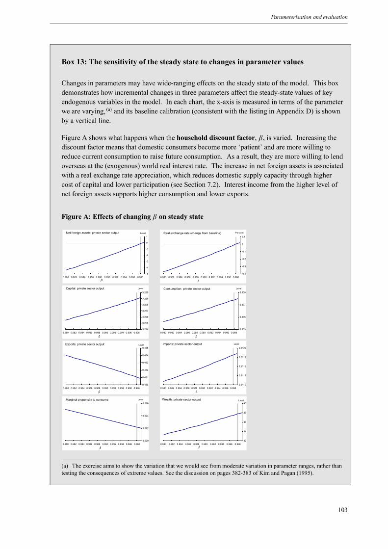
Parameterisation and evaluation
Box 13: The sensitivity of the steady state to changes in parameter values
Changes in parameters may have wide-ranging effects on the steady state of the model. This boxdemonstrates how incremental changes in three parameters affect the steady-state values of keyendogenous variables in the model. In each chart, the x-axis is measured in terms of the parameterwe are varying, (a) and its baseline calibration (consistent with the listing in Appendix D) is shownby a vertical line.
Figure A shows what happens when the household discount factor, β, is varied. Increasing thediscount factor means that domestic consumers become more ‘patient’ and are more willing toreduce current consumption to raise future consumption. As a result, they are more willing to lendoverseas at the (exogenous) world real interest rate. The increase in net foreign assets is associatedwith a real exchange rate appreciation, which reduces domestic supply capacity through highercost of capital and lower participation (see Section 7.2). Interest income from the higher level ofnet foreign assets supports higher consumption and lower exports.
Figure A: Effects of changing β on steady state
Real exchange rate (change from baseline)
-0.4
-0.3
-0.2
-0.1
0
0.1
0.980 0.982 0.984 0.986 0.988 0.990 0.992 0.994 0.996 0.998
Per cent
β
Net foreign assets: private sector output
-5
-4
-3
-2
-1
0
1
0.980 0.982 0.984 0.986 0.988 0.990 0.992 0.994 0.996 0.998
Level
β
Capital: private sector output
3.224
3.225
3.226
3.227
3.228
3.229
3.230
0.980 0.982 0.984 0.986 0.988 0.990 0.992 0.994 0.996 0.998
Level
β
Consumption: private sector output
0.833
0.835
0.837
0.839
0.980 0.982 0.984 0.986 0.988 0.990 0.992 0.994 0.996 0.998
Level
β
Exports: private sector output
0.480
0.481
0.482
0.483
0.484
0.485
0.980 0.982 0.984 0.986 0.988 0.990 0.992 0.994 0.996 0.998
Level
β
Imports: private sector output
0.5110
0.5113
0.5116
0.5119
0.5122
0.980 0.982 0.984 0.986 0.988 0.990 0.992 0.994 0.996 0.998
Level
β
Marginal propensity to consume
0.020
0.022
0.024
0.026
0.980 0.982 0.984 0.986 0.988 0.990 0.992 0.994 0.996 0.998
Level
β
Wealth: private sector output
32
34
36
38
40
0.980 0.982 0.984 0.986 0.988 0.990 0.992 0.994 0.996 0.998
Level
β
(a) The exercise aims to show the variation that we would see from moderate variation in parameter ranges, rather thantesting the consequences of extreme values. See the discussion on pages 382-383 of Kim and Pagan (1995).
103
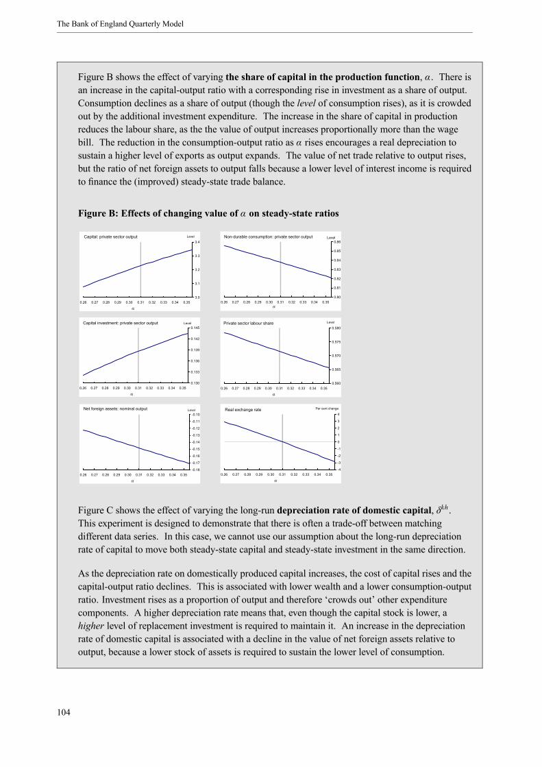
The Bank of England Quarterly Model
Figure B shows the effect of varying the share of capital in the production function, α. There isan increase in the capital-output ratio with a corresponding rise in investment as a share of output.Consumption declines as a share of output (though the level of consumption rises), as it is crowdedout by the additional investment expenditure. The increase in the share of capital in productionreduces the labour share, as the the value of output increases proportionally more than the wagebill. The reduction in the consumption-output ratio as α rises encourages a real depreciation tosustain a higher level of exports as output expands. The value of net trade relative to output rises,but the ratio of net foreign assets to output falls because a lower level of interest income is requiredto finance the (improved) steady-state trade balance.
Figure B: Effects of changing value of α on steady-state ratios
Non-durable consumption: private sector output
0.80
0.81
0.82
0.83
0.84
0.85
0.86
0.26 0.27 0.28 0.29 0.30 0.31 0.32 0.33 0.34 0.35
Level
α
Capital: private sector output
3.0
3.1
3.2
3.3
3.4
0.26 0.27 0.28 0.29 0.30 0.31 0.32 0.33 0.34 0.35
Level
α
Capital investment: private sector output
0.130
0.133
0.136
0.139
0.142
0.145
0.26 0.27 0.28 0.29 0.30 0.31 0.32 0.33 0.34 0.35
Level
α
Private sector labour share
0.560
0.565
0.570
0.575
0.580
0.26 0.27 0.28 0.29 0.30 0.31 0.32 0.33 0.34 0.35
Level
α
Real exchange rate
-4
-3
-2
-1
0
1
2
3
4
0.26 0.27 0.28 0.29 0.30 0.31 0.32 0.33 0.34 0.35
Per cent change
α
Net foreign assets: nominal output
-0.18
-0.17
-0.16
-0.15
-0.14
-0.13
-0.12
-0.11
-0.10
0.26 0.27 0.28 0.29 0.30 0.31 0.32 0.33 0.34 0.35
Level
α
Figure C shows the effect of varying the long-run depreciation rate of domestic capital, δkh .This experiment is designed to demonstrate that there is often a trade-off between matchingdifferent data series. In this case, we cannot use our assumption about the long-run depreciationrate of capital to move both steady-state capital and steady-state investment in the same direction.
As the depreciation rate on domestically produced capital increases, the cost of capital rises and thecapital-output ratio declines. This is associated with lower wealth and a lower consumption-outputratio. Investment rises as a proportion of output and therefore ‘crowds out’ other expenditurecomponents. A higher depreciation rate means that, even though the capital stock is lower, ahigher level of replacement investment is required to maintain it. An increase in the depreciationrate of domestic capital is associated with a decline in the value of net foreign assets relative tooutput, because a lower stock of assets is required to sustain the lower level of consumption.
104
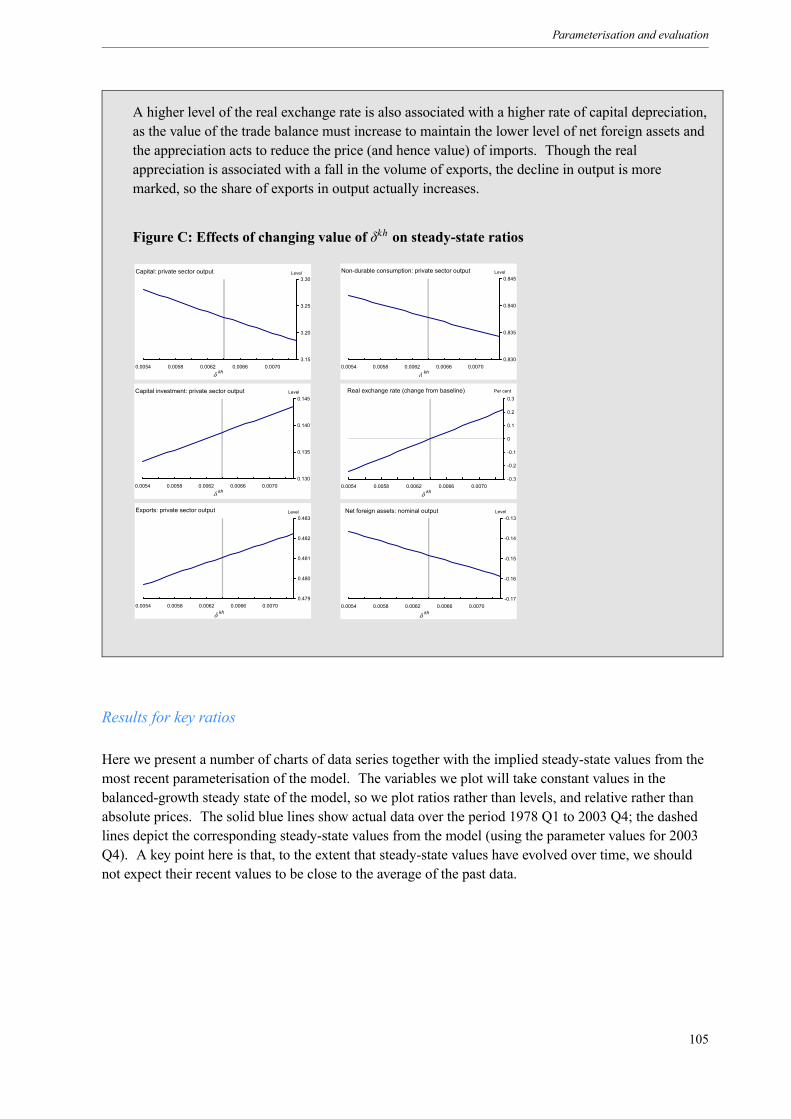
Parameterisation and evaluation
A higher level of the real exchange rate is also associated with a higher rate of capital depreciation,as the value of the trade balance must increase to maintain the lower level of net foreign assets andthe appreciation acts to reduce the price (and hence value) of imports. Though the realappreciation is associated with a fall in the volume of exports, the decline in output is moremarked, so the share of exports in output actually increases.
Figure C: Effects of changing value of δkh on steady-state ratios
Non-durable consumption: private sector output
0.830
0.835
0.840
0.845
0.0054 0.0058 0.0062 0.0066 0.0070
LevelCapital: private sector output
3.15
3.20
3.25
3.30
0.0054 0.0058 0.0062 0.0066 0.0070
Level
δ kh
Capital investment: private sector output
0.130
0.135
0.140
0.145
0.0054 0.0058 0.0062 0.0066 0.0070
Level
Exports: private sector output
0.479
0.480
0.481
0.482
0.483
0.0054 0.0058 0.0062 0.0066 0.0070
Level
Real exchange rate (change from baseline)
-0.3
-0.2
-0.1
0
0.1
0.2
0.3
0.0054 0.0058 0.0062 0.0066 0.0070
Per cent
Net foreign assets: nominal output
-0.17
-0.16
-0.15
-0.14
-0.13
0.0054 0.0058 0.0062 0.0066 0.0070
Level
δ kh
δ kh
δ kh δ kh
δ kh
Results for key ratios
Here we present a number of charts of data series together with the implied steady-state values from themost recent parameterisation of the model. The variables we plot will take constant values in thebalanced-growth steady state of the model, so we plot ratios rather than levels, and relative rather thanabsolute prices. The solid blue lines show actual data over the period 1978 Q1 to 2003 Q4; the dashedlines depict the corresponding steady-state values from the model (using the parameter values for 2003Q4). A key point here is that, to the extent that steady-state values have evolved over time, we shouldnot expect their recent values to be close to the average of the past data.
105
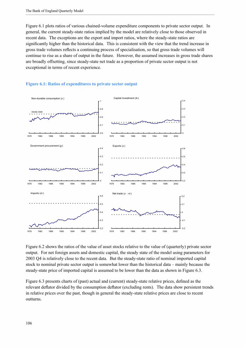
The Bank of England Quarterly Model
Figure 6.1 plots ratios of various chained-volume expenditure components to private sector output. Ingeneral, the current steady-state ratios implied by the model are relatively close to those observed inrecent data. The exceptions are the export and import ratios, where the steady-state ratios aresignificantly higher than the historical data. This is consistent with the view that the trend increase ingross trade volumes reflects a continuing process of specialisation, so that gross trade volumes willcontinue to rise as a share of output in the future. However, the assumed increases in gross trade sharesare broadly offsetting, since steady-state net trade as a proportion of private sector output is notexceptional in terms of recent experience.
Figure 6.1: Ratios of expenditures to private sector output
Non-durable consumption (c )
0.6
0.7
0.8
0.9
1
1978 1982 1986 1990 1994 1998 2002
steady state
Capital investment (ik )
0
0.1
0.2
0.3
0.4
1978 1982 1986 1990 1994 1998 2002
Government procurement (g )
0
0.1
0.2
0.3
0.4
1978 1982 1986 1990 1994 1998 2002
Exports (x )
0.2
0.3
0.4
0.5
0.6
1978 1982 1986 1990 1994 1998 2002
Imports (m )
0.2
0.3
0.4
0.5
0.6
1978 1982 1986 1990 1994 1998 2002
Net trade (x - m )
-0.2
-0.1
0
0.1
0.2
1978 1982 1986 1990 1994 1998 2002
Figure 6.2 shows the ratios of the value of asset stocks relative to the value of (quarterly) private sectoroutput. For net foreign assets and domestic capital, the steady state of the model using parameters for2003 Q4 is relatively close to the recent data. But the steady-state ratio of nominal imported capitalstock to nominal private sector output is somewhat lower than the historical data – mainly because thesteady-state price of imported capital is assumed to be lower than the data as shown in Figure 6.3.
Figure 6.3 presents charts of (past) actual and (current) steady-state relative prices, defined as therelevant deflator divided by the consumption deflator (excluding rents). The data show persistent trendsin relative prices over the past, though in general the steady-state relative prices are close to recentoutturns.
106
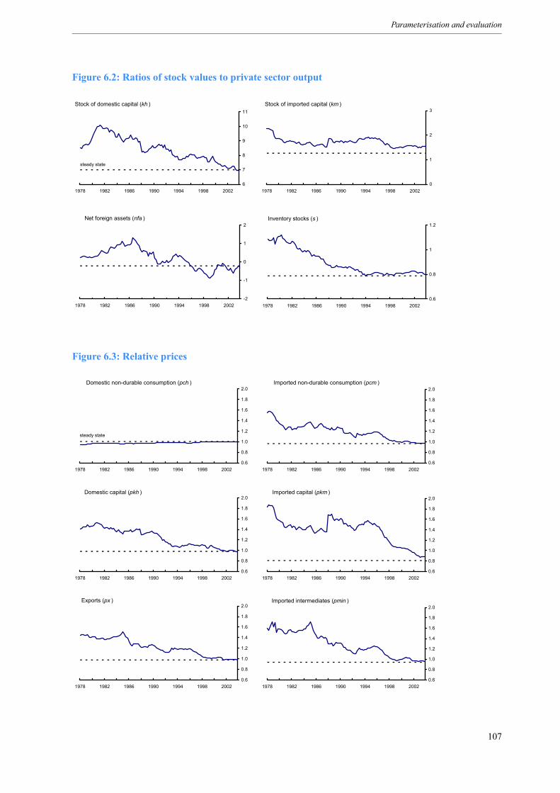
Parameterisation and evaluation
Figure 6.2: Ratios of stock values to private sector output
Net foreign assets (nfa )
-2
-1
0
1
2
1978 1982 1986 1990 1994 1998 2002
Stock of domestic capital (kh )
6
7
8
9
10
11
1978 1982 1986 1990 1994 1998 2002
steady state
Stock of imported capital (km )
0
1
2
3
1978 1982 1986 1990 1994 1998 2002
Inventory stocks (s )
0.6
0.8
1
1.2
1978 1982 1986 1990 1994 1998 2002
Figure 6.3: Relative prices
Domestic non-durable consumption (pch )
0.6
0.8
1.0
1.2
1.4
1.6
1.8
2.0
1978 1982 1986 1990 1994 1998 2002
steady state
Imported non-durable consumption (pcm )
0.6
0.8
1.0
1.2
1.4
1.6
1.8
2.0
1978 1982 1986 1990 1994 1998 2002
Domestic capital (pkh )
0.6
0.8
1.0
1.2
1.4
1.6
1.8
2.0
1978 1982 1986 1990 1994 1998 2002
Imported capital (pkm )
0.6
0.8
1.0
1.2
1.4
1.6
1.8
2.0
1978 1982 1986 1990 1994 1998 2002
Exports (px )
0.6
0.8
1.0
1.2
1.4
1.6
1.8
2.0
1978 1982 1986 1990 1994 1998 2002
Imported intermediates (pmin )
0.6
0.8
1.0
1.2
1.4
1.6
1.8
2.0
1978 1982 1986 1990 1994 1998 2002
107

The Bank of England Quarterly Model
6.3.3 Parameterising the core dynamics
As noted above, some parameters affect both the steady state and the dynamic properties of the model.For example, depreciation rates affect steady-state stock ratios as well as the amplitude and rate of decayof the investment boost that follows a permanent increase in the desired level of capital.
We also have a set of parameters in the core model that affect only the dynamic behaviour of the model.These include: consumers’ habits; capital and investment adjustment costs; inventory stock adjustmentcosts; the elasticity of capital utilisation; nominal price and wage stickiness; and nominal wage and priceindexation parameters. These parameters can be set to generate a model with a fully flexibleequilibrium in which quantities and prices are free to adjust immediately in the face of a shock.
As with the calibration of the steady state, our approach to setting of these parameters has been largelyinformal. We have used three main exercises to judge how to set them: first, historical fit against thedata; second, responses to marginal shocks (such as those shown in Chapter 7); and third, the estimationresults from the non-core equations, which can be viewed as a statistical assessment of the degree towhich the core model can capture the properties of the historical data.
The process for setting the parameters was iterative. The starting values represented our priors withwhich we evaluated the model using the three criteria (fit, shock responses and non-core results) beforeadjusting the parameter values in the light of the results. Clearly this process is very informal, since‘trial and error’ adjustment of parameters does not guarantee values that best meet our criteria.Moreover, while each criterion can be summarised by some kind of formal metric, (39) the weightsapplied to each are essentially judgemental.
The starting values (or priors) come from two main sources. First, some parameters have plausiblevalues when interpreted literally. For example, if wage stickiness is implemented using Calvo contracts,the adjustment probability determines the expected duration of contracts and a plausible length for theaverage wage contract implies a specific value of the adjustment probability. Second, we can useestimation results from previous studies.
There are potential problems with both of these approaches. Literal interpretation of parameters maynot be appropriate, as the core theory is a highly stylised representation of reality. And the directrelevance of existing estimates is often unclear: the precise data sources may not be directly comparable;existing estimates are usually conditional on the assumed structure of a model, which may differ fromBEQM; and not all empirical evidence is based on UK data, and parameters may vary across countries.For example, parameters that relate to the costs of adjusting prices could take guidance from estimates ofNew Keynesian Phillips curves (relating inflation to expected future inflation and real marginal costs).But the results of estimation using, say, CPI inflation may not be of direct use in choosing parametersthat affect price setting at a more disaggregated level, as in BEQM. Similarly, some estimatedparameters may not be of direct use if based on a different assumption about the production technologyto that employed in BEQM. This problem applies even more forcefully to microeconomic studies,which often allow for important roles for factors that are ignored or highly simplified in macroeconomicmodels (for example heterogeneity and uncertainty). (40)
(39)See the discussion in Section 6.3.4. When matching impulse responses, the metric could (in principle) be in terms ofsquared deviations from specific shock responses. When fitting the data, we could (in principle) use the likelihood function asthe metric.(40)Such difficulties are summarised succinctly on page 546 of Browning et al (1999): ‘A parameter that is valid for a modelin one economic environment cannot be uncritically applied to a model embedded in a different economic environment’.
108

Parameterisation and evaluation
Before discussing the parameter choices in detail, a summary of some of the main conclusions is asfollows:• habits and capital adjustment costs are needed to generate inertia in real variables;• nominal wage stickiness and substantial nominal price stickiness are needed to ensure that supplyresponds elastically to movements in demand; (41)
• we need to allow lagged nominal price and wage inflation to influence price and wage setting, sothat inflation builds up gradually, rather than jumping immediately after a shock;
• the strength of the response of inflation relative to output depends on the slope of the short-runmarginal cost curve. Variable capital utilisation is also needed to ensure that supply respondselastically to movements in demand. Otherwise, even with substantial nominal wage and pricestickiness, the incentive for firms to change prices rather than quantities is large; and
• substantial import price stickiness is required to ensure that exchange rate changes are passedthrough gradually into consumer price inflation. We also assume a degree of dependence on pastimport price inflation, which slows down the rate of pass-through.
The discussion below is ordered according to generic groups of rigidities affecting demand, supply andnominal prices and wages. A full listing of parameter values can be found in Appendix D. We considerevidence using data from different countries, different samples and employing different modellingassumptions. As noted above, these issues make it difficult to assess the relevance to parameter choicesfor BEQM, so we do not comment on the implications of all discrepancies between our parameterchoices and the range of available empirical estimates.
First we look at parameters influencing demand behaviour. The value set for the elasticity ofintertemporal substitution for consumption in utility (42) is relatively low (σ c = 0.2) compared with thelogarithmic utility assumption (σ c = 1) favoured in many real business cycle calibrations. (43) A lowelasticity of intertemporal substitution implies (other things being equal) that consumers are less willingto substitute consumption across time in response to a temporary change in real interest rates. The rangeof empirical estimates is very wide for this parameter, coming from different countries, data sets andsample periods. (44) Indeed, Smets and Wouters (2004) obtain a estimate of around 0.6 using US data,compared with around 0.35 from Edge et al (2003). The single equation estimate of Nelson andNikolov (2002) based on UK data suggests a value of at least 0.34, whereas the full model estimate ofBergin (2003) suggests a value very close to zero.
Our assumptions about habit formation imply that an individual’s current utility places some weight onpast consumption: ψhab = ψhabd = 0.7. (45) Habit formation means that consumers gain utility fromkeeping consumption close to previous levels, which can introduce inertia into the response ofconsumption to temporary shocks. Studies using slightly different formulations of the utility function
(41)Some studies, for example Christiano, Eichenbaum and Evans (2001), find that nominal wage stickiness alone is sufficient.These authors note, however, that their result is conditional on the assumption of low marginal costs of changing capitalutilisation. Our finding, that nominal price stickiness is also needed, is more in accord with Smets and Wouters (2003a).(42)Note that this parameter does not only affect the dynamic responses of the core model – it will also affect the steady statethrough its influence on the marginal propensity to consume.(43)The imposition of a balanced growth steady state with endogenous labour supply may restrict the class of preferences thatcan be used (an example is to assume logarithmic utility in consumption). We are not constrained in our choice because of theway in which we implement participation decisions.(44)See Cromb and Fernandez-Corugedo (2004).(45)When ψhab = 0, an individual’s current utility does not depend on the habit variable (in BEQM a function of past percapita consumption). When ψhab = 1, utility in BEQM is defined in terms of the ratio of individual consumption to past (percapita) consumption. Our parameterisation is therefore towards the latter specification of utility. See Box 2 on page 30 for theprecise specification of the utility function.
109
The Bank of England Quarterly Model
have often found a role for habit formation. (46) For example, Smets and Wouters (2003a) find a valueclose to 0.6 for euro-area data; Smets and Wouters (2004) find a value slightly higher than 0.6 for USdata; and Juillard et al (2004) estimate a value around 0.8 for US data. Banerjee and Batini (2003) findestimates of around 0.8 using UK data, with a similar utility function but a slightly differentspecification for the habit variable.
Turning to supply, our parameterisation imposes significant costs of adjusting capital, which reduce thefirm’s incentive to change the capital stock in response to changes in the cost of capital. The particularvalues of the adjustment cost parameters for home and imported capital (χ kh and χ km) are notparticularly informative, since they are conditional on the precise specification of the costs. To aidcomparisons across models, such parameters are often converted into a more useful metric – forexample, the proportion of any immediate increase in investment that must be paid in adjustment costs,starting from a steady state. Our parameterisation implies that increasing home capital investment by1% above the steady-state rate leads to a cost of around 0.005% of steady-state home investment. (47)
For imported capital, the cost is around 0.003% of imported investment. Estimates from other studiessuggest costs of 0.009% (Edge et al (2003)) and 0.018% (Christiano et al (2001)) based on US data and0.034% for euro-area data (Smets and Wouters (2003a)). (48) Using a capital adjustment costformulation similar to the one employed in BEQM, Bergin (2003) estimates a cost of around 0.22% onUK data. The parameterisation for costs of adjusting dwellings investment implies that increasingdwellings investment by 1% from steady state incurs a cost of 0.05% of steady state dwellingsinvestment. (49) The adjustment cost specification in BEQM also allows capital adjustment costs todepend partly on lagged changes in the capital stock (with a weight of kh = km = 0.7) and partly ontrend growth (with a weight of 0.3). The above studies using US and euro-area data use an adjustmentcost specification better approximated by kh = km = 1.
Variable intensity of capital utilisation is an important feature of the core theory, which effectively‘flattens’ the real marginal cost curve so that meeting changes in demand is possible without requiringlarge changes in marginal costs that would other things being equal, imply large price changes. (50) Mostof the comparator studies do not employ the same type of adjustment cost function for changes inutilisation that we use in BEQM. This makes comparisons less straightforward, but a qualitative featureof the studies is that they tend to find that the elasticity of the cost with respect to utilisation is relativelylow (generally much lower than that implied by a quadratic cost function). The BEQM core modelassumes that effective depreciation rates for home and imported capital are adjusted by a correction forutilisation (z) with an elasticity φz = 0.1. Estimates for this parameter by Basu and Kimball (1997),(46)Generally the studies quoted here assume that utility depends on the difference between individual consumption and thehabit variable, rather than the ratio as we assume in BEQM. However, the Euler equations implied by these two specificationsare broadly similar (to a log-linear approximation as used in those studies) in terms of the coefficients on future and pastconsumption.(47)We can calculate this cost as follows. The form of the adjustment cost implies that, close to the steady state, the cost as a
proportion of steady-state investment is χ2KK
2 KI = χ
2KK
2δ−1, where the equality follows from the fact that
steady-state investment covers capital depreciation. If the rate of investment increases by 1% above the steady-state rate thenthe capital stock increases by K = 0.01δK . This implies that the cost as a proportion of steady-state investment isχ2 [0.01]
2 δ.(48)These figures are based on the analysis of Edge et al (2003) who report an investment adjustment cost function that
specifies net (of adjustment cost) investment as exp −χ2 II
2I which means that the cost as a proportion of investment is:
1− exp −χ2 0.012 . They report their estimate of χ and compare this directly with the parameter estimates in other studies.(49)The costs in this case take the form χ
2I DI D
2I D so that the cost of increasing investment by 1% above steady state, as a
ratio of investment, is χ2 [0.01]2.
(50)See Christiano et al (2001).
110
Parameterisation and evaluation
based on US data, imply a very large confidence interval centred on a value of around unity. (51) Baxterand Farr (2001) find that a calibrated value of this elasticity of 0.1 improves the ability of aninternational real business cycle model to match certain properties of the data compared with thebenchmark calibration of unity.
Our parameterisation implies that labour adjustment costs are absent: χ l = 0. We assume that averagehours worked are exogenous to the firm’s decision process and cannot respond to shocks. The othercomponent of total hours worked is employment in heads – making this slow to adjust (χ l > 0) wouldsteepen the real marginal cost schedule, which would tend to offset the beneficial effects of variablecapital utilisation described above. The responsiveness of participation to changes in the wage rate thatcan be expected to be earned from labour market activity is relatively low: the elasticity of participationwith respect to the real wage is ηl = 0.1. The estimation results on UK data by Bergin (2003) suggestan elasticity with respect to the wage rate very close to zero. Other estimates suggest higher values:Smets and Wouters (2004) estimate an elasticity around 0.5 for US data and Smets and Wouters (2003a)obtain an estimate close to 0.4 for the euro area.
We implement nominal rigidities in two ways: as discussed in Chapter 3, we use Rotemberg (1982)adjustment costs for prices set by domestic firms and a Calvo (1983) specification for nominal wagesand import prices. To make the comparison more straightforward we convert our Rotemberg adjustmentcost parameter settings into the equivalent Calvo adjustment probabilities. (52) Our parameterisationimplies that the Calvo probability of adjusting prices for domestically produced consumption, capitaland government procurement is around 0.15. The associated probability for export prices is around 0.4.This reflects the fact that we assume price stickiness in the foreign currency price of exports, which is arelatively volatile data series. We assume that dwellings prices are perfectly flexible (χd = 0). Theadjustment probabilities for import (consumption, investment and intermediates) prices are close tothose for domestic prices at 0.15. Other studies estimate a variety of different adjustment probabilitiesfor prices. For the United States, Christiano et al (2001) estimate a probability of 0.5; Edge et al (2003)find 0.33; (53) and Smets and Wouters (2004) estimate a value of 0.1. For the euro area, Smets andWouters (2003a) estimate a value of 0.1. Also using euro area data, Adolfson et al (2004b) estimateprobabilities of 0.12, 0.73, 0.44 and 0.34 for domestic prices, imported consumption prices, importedinvestment prices and export prices respectively. And Bergin (2003) estimates a probability of 0.06using UK data. (54)
As well as parameters governing the extent of price stickiness (such as χ pch) the core model alsoincludes parameters (such as pchdot ) that determine the extent to which price adjustment costs areinfluenced by lagged inflation. For domestic prices (home consumption, home capital and governmentprocurement) and exports, we assume that adjustment costs place a 50% weight on lagged inflation( pchdot = pkhdot = pgdot = pxdot = 0.5). For import prices, past inflation rates are assumed to playmore of a role in determining adjustment costs: we set pcmdot = pkmdot = pmindot = 0.9. Thespecification of Edge et al (2003) allows for separate identification of a parameter measuring thedependence of adjustment costs on lagged inflation. Their results using US data suggest little role for
(51)The 95% confidence interval they report is [-0.2,2].(52)We do this by noting the well known property that, under the assumptions defining the firm’s maximisation problem, thelog-linearised pricing equations have the same reduced form as a Calvo approach. The parameters linked by the equationη−1χ = (1−βζ)(1−ζ )
ζ , where η is the demand elasticity, χ is the Rotemberg adjustment cost, β is the household discount factorand (1− ζ ) is the Calvo adjustment probability. In our calculations we assume β = 0.99, which is the standard calibration inthe papers we use to compare estimates.(53)Here we use the formula mentioned in the footnote above to convert the adjustment cost estimate into a Calvo probability.(54)Here we use the formula mentioned in the footnote above to convert the adjustment cost estimate into a Calvo probability.
111
The Bank of England Quarterly Model
lagged inflation in price adjustment costs. The results of Smets and Wouters (2004) on US data suggesta weight (for domestic price setting) of around 0.47. (55) For the euro area, Smets and Wouters (2003a)also estimate a weight of 0.47 for domestic prices and Adolfson et al (2004b) estimate weights of 0.21and 0.15 for domestic prices and export prices respectively.
Nominal wage stickiness is implemented according to a Calvo scheme. The parameterisation sets theadjustment probability at 0.5. Using US data, Christiano et al (2001) estimate a probability of 0.3.andSmets and Wouters (2004) find an estimate of 0.2. For the euro area, Smets and Wouters (2003a)estimate a probability of 0.26 and Adolfson et al (2004b) find 0.30. The type of Calvo mechanism usedin the core model allows the specification of an indexation factor, which specifies the extent to whichunadjusted private sector nominal wage contracts are uprated in line with lagged average (private sector)wage inflation. Our parameterisation of wdot = 0.9 implies that a high weight is placed on lagged wageinflation. Smets and Wouters (2004) estimate a weight on lagged inflation of around 0.32 using US data.For the euro area, Smets and Wouters (2003a) estimate a value of 0.76 and Adolfson et al (2004b)estimate 0.51.
6.3.4 More formal approaches
The procedure described above is by no means the only possible approach. There is now a substantialliterature that attempts to formalise the traditional approaches to parameterisation. For example, theexercise in Box 13 on page 103 could be extended to estimate sampling uncertainty, which is lacking ininformal calibration exercises. (56) As several authors have noted, calibration amounts to imposingmoment conditions and, in theory, can be formalised in a way analogous to GMM estimators. Severalpapers have used the state-space form of a model to relate to VARs, (57) or to deduce key modelproperties. (58) There are problems in applying these approaches to a model as large as BEQM, but it ispossible to work out ways by which a large system (the theoretical model) can be formally related tosmaller systems, which can then be directly related to the data. (59)
There has also been considerable progress in recent years in directly estimating the underlyingparameters of micro-founded models by maximum likelihood methods. In theory, the state-spacerepresentation of the model can be used to provide prediction errors, and so a likelihood function can beevaluated. In practice, however, the likelihood surface is usually relatively flat and numerical searchmethods will not converge or will converge on local maxima. Bayesian priors can be used to assistestimation, (60) but Bayesian maximum likelihood has not yet been applied to systems are large asBEQM.(61) Nevertheless, the technology is developing rapidly and it may prove possible to use suchtechniques in future: they have been applied to increasingly large systems as developments have beenmade in numerical methods. (62)
(55)This study uses a Calvo mechanism for price stickiness. However, the log-linearised pricing equations from both theRotemberg and Calvo pricing mechanisms imply that Smets and Wouters’ parameter γ p can be interpreted analogously to theparameters reported in the main text.(56)See Canova (1994, 1995); for an application to a large model see Amano et al (2002).(57)See, for example, Ingram and Whiteman (1994).(58)See, for example, Watson (1993).(59)See Kapetanios et al (2004).(60)See, for example, Schorfheide (1999) and Fernández-Villaverde and Rubio-Ramírez (2004).(61)No use is made in the core model of so-called ‘extrinsic dynamics’ (ie persistent shock processes) to bolster the fit of themodel.(62)See the pioneering work by Smets and Wouters (2003a). More recently, some relatively large systems have beenestimated; see Adolfson et al (2004a).
112
Parameterisation and evaluation
6.4 Parameterising the non-core equations
As described in Chapter 4, the non-core equations pick up correlations in the data that are not explainedby the theory set out in Chapter 3. In effect, we can think of these equations as modelling the gapbetween the core model and the historical data.
6.4.1 Estimating the non-core equations
Generating core model paths
As described in Chapter 5, we generate core model paths by running the core model as a full system.Simulating the core model over the past requires us to make two important choices: first, how to treatvalues of predetermined variables; and second, what information to assume was available to agents ateach date in the past when generating the core solution.
Given values for the predetermined variables, the core model generates paths for endogenous variablesthat converge on the steady state. The path of the predetermined variables forms part of this core modelsolution: for example, the path of the capital stock is given by accumulated investment flows. Oneoption would be to give the core model the values of predetermined variables at the start of the historicalsample and allow the solutions for these variables to be given by the relationships in the core model. Soin this case, the core model solution for the capital stock would equal the initial value of the capital stockobserved in the data at the start of sample, plus cumulated net investment from the core model.However, we choose to update the values of the predetermined variables from the data: core modelsolutions in period t depend on the data for the capital stock at period t − 1, as discussed in Section5.1.1. This means that the core model solutions for the historical data period represent a sequence ofone-period projections, conditional on the data up to the previous period. As such, the core model isallowed to react to news in both exogenous variables and changes in the predetermined endogenousvariables. (63)
The second choice concerns the amount of information about the future that we assume is available ineach period of the historical sample. This is important because, in each period, the path of the coremodel depends on the expected future path of exogenous variables. One assumption would be to allowperfect foresight of exogenous variables over the historical sample: in each past period, we would allowagents in the core model to observe the actual path of exogenous variables in the full data set. Thisassumption is straightforward, but not realistic for many variables. Instead, we assume that expectationsof future exogenous variables are generated by an ‘exogenous variables model’. As described in Box 10on page 78, this approach assumes that agents in the core model decompose movements in exogenousvariables into permanent and transitory components and forecast how the exogenous variable returns toits permanent level. In general, we use a low-frequency filter to identify the permanent component andthen estimate a simple time-series process for the transitory component. However, judgement is alsoapplied where appropriate. (64)
(63)One way of thinking about this is that the core model is repeatedly ‘surprised’ when the data for predetermined variablesturn out differently to what was decided upon last period. These surprises represent shocks to the model and in response agentsformulate new optimal plans in each period.(64)For example, when tax changes are pre-announced, we may want to ensure that this news is contained in the permanentcomponent of the tax rate from the announcement date.
113
The Bank of England Quarterly Model
Equation form
The equations we estimate takes the general form of equation (4.3) in Chapter 4, which we repeat herefor convenience.
yt = − (1− α1) yt−1 − ycoret−1 + β1 ycoret + ψ1zt + εt
In general, the we found the β1 coefficients to be insignificantly different from zero and so terms inycore do not appear in the estimated non-core equations presented in Section 6.4.2. Our specification
has the advantage of smoothing through the initial responses of the core model. Even though the coremodel contains extensive real and nominal inertia, endogenous variables can still jump in response todisequilibrium between starting points and equilibrium targets. A primary role of the non-coreequations is therefore to allow for an extra layer of persistence to forecasts of a sort that is, as yet,difficult to capture by micro-founded dynamic optimising models.
Lags and proxy variables
One way of approaching the estimation of non-core equations would be to try to specify the best singleequation for each variable. We could imagine a process in which we began with a very generalspecification of each equation (with many lagged dependent variables and proxy variables) and testeddown to a preferred equation. Such an approach is likely to lead to a set of non-core equations eachcontaining a relatively large number of lagged dependent variables and proxy variables. Thoughindividually these equations would have sound properties (for example, high measures of fit such as R2
statistics) they may not perform at all well when combined as a system to produce forecasts. One reasonis that the inclusion of a large number of proxy variables means that these too must be forecast and thatcan affect the overall forecasting performance of the system. Another reason is that the interaction ofequations with large numbers of lagged dependent variables can lead to implausible system-wideproperties.
Section 2.2 discussed the trade-off between theoretical consistency and data coherence, illustrated in astylised form in Figure 2.1 – our approach to estimating the non-core equations can be seen as reflectingour choice as to which part of the frontier we should aim for. In particular, we follow a strategy that isconsistent with the remit of the model development project to improve theoretical coherence and fit thedata at least as well as the previous MTMM model. We start with the core model and parsimoniouslyadd non-core dynamics to improve the empirical properties of the full model. (65) At the limit, we couldimagine a case in which the core theory was sufficiently rich that it did not require any additionalnon-core equations. In practice, we do find that lagged dependent variables and proxy variables areuseful. Proxy variables are selected, based on a view of what is known to be missing in the core theory,the evidence gained from using the previous MTMM model in forecasting, and specialists’ conjuncturalexperiences. In general, we find that changes in aggregate activity variables (such as output orunemployment) are necessary to pick up accelerator-like effects. (66) Changes in nominal variables (suchas interest rates and prices) are also useful; we cautiously interpret those as picking up credit-relatedeffects. However, in terms of the simulation responses seen in Chapter 7, these effects are not verypowerful.
(65)An alternative, statistical, argument for parsimony is that while inclusion of a relevant variable may improve the accuracyof the forecast mean (and hence reduce bias) it will also increase parameter uncertainty (and so add to the forecast errorvariance). It is possible, therefore, that a misspecified but parsimonious model can out-forecast the data generating process.(66)We hesitate to interpret this literally as evidence for accelerator mechanisms, as they can easily arise in the reduced formsof neoclassical rational expectations models, especially when data are subject to mismeasurement: see, for example, Sargent(1989).
114
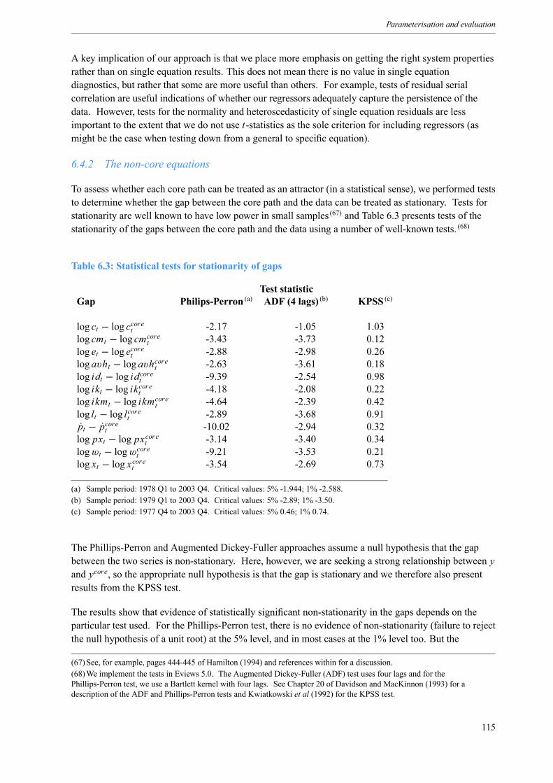
Parameterisation and evaluation
A key implication of our approach is that we place more emphasis on getting the right system propertiesrather than on single equation results. This does not mean there is no value in single equationdiagnostics, but rather that some are more useful than others. For example, tests of residual serialcorrelation are useful indications of whether our regressors adequately capture the persistence of thedata. However, tests for the normality and heteroscedasticity of single equation residuals are lessimportant to the extent that we do not use t-statistics as the sole criterion for including regressors (asmight be the case when testing down from a general to specific equation).
6.4.2 The non-core equations
To assess whether each core path can be treated as an attractor (in a statistical sense), we performed teststo determine whether the gap between the core path and the data can be treated as stationary. Tests forstationarity are well known to have low power in small samples (67) and Table 6.3 presents tests of thestationarity of the gaps between the core path and the data using a number of well-known tests. (68)
Table 6.3: Statistical tests for stationarity of gaps
Test statisticGap Philips-Perron (a) ADF (4 lags) (b) KPSS (c)
log ct − log ccoret -2.17 -1.05 1.03log cmt − log cmcoret -3.43 -3.73 0.12log et − log ecoret -2.88 -2.98 0.26log avht − log avhcoret -2.63 -3.61 0.18log idt − log idcoret -9.39 -2.54 0.98log ikt − log ikcoret -4.18 -2.08 0.22log ikmt − log ikmcoret -4.64 -2.39 0.42log lt − log lcoret -2.89 -3.68 0.91pt − pcoret -10.02 -2.94 0.32log pxt − log pxcoret -3.14 -3.40 0.34logwt − logwcoret -9.21 -3.53 0.21log xt − log xcoret -3.54 -2.69 0.73
(a) Sample period: 1978 Q1 to 2003 Q4. Critical values: 5% -1.944; 1% -2.588.(b) Sample period: 1979 Q1 to 2003 Q4. Critical values: 5% -2.89; 1% -3.50.(c) Sample period: 1977 Q4 to 2003 Q4. Critical values: 5% 0.46; 1% 0.74.
The Phillips-Perron and Augmented Dickey-Fuller approaches assume a null hypothesis that the gapbetween the two series is non-stationary. Here, however, we are seeking a strong relationship between yand ycore, so the appropriate null hypothesis is that the gap is stationary and we therefore also presentresults from the KPSS test.
The results show that evidence of statistically significant non-stationarity in the gaps depends on theparticular test used. For the Phillips-Perron test, there is no evidence of non-stationarity (failure to rejectthe null hypothesis of a unit root) at the 5% level, and in most cases at the 1% level too. But the
(67)See, for example, pages 444-445 of Hamilton (1994) and references within for a discussion.(68)We implement the tests in Eviews 5.0. The Augmented Dickey-Fuller (ADF) test uses four lags and for thePhillips-Perron test, we use a Bartlett kernel with four lags. See Chapter 20 of Davidson and MacKinnon (1993) for adescription of the ADF and Phillips-Perron tests and Kwiatkowski et al (1992) for the KPSS test.
115
The Bank of England Quarterly Model
Augmented Dickey-Fuller (ADF) test shows some evidence of non-stationarity (failure to reject the nullhypothesis of a unit root) for consumption, dwellings investment, total and imported capital investmentand exports. And the KPSS test suggests evidence of non-stationarity (here, by rejection of nullhypothesis of stationarity) for consumption, dwellings investment, participation and exports.
Consumption
The non-core equation contains an error correction to non-durable consumption. An extra argument inassets is included to ensure convergence in net foreign assets (see Section 4.2.2). Proxy variables foreffects missing from the core include changes in the value of the housing stock, as a proxy for housingcollateral effects; changes in household income, as a proxy for the existence of rule-of-thumbindividuals; changes in the employment rate, as a proxy for confidence and uncertainty effects; andchanges in nominal interest rates, as a proxy for credit and cash-flow effects.
log ct = 0.197(0.699)
log eaggt − 1.125(2.203)
rgt + 0.221(2.316)
log lyt + 0.194(3.872)
log(phsetdt−1)
− 0.125(3.077)
(log ct−1 − log ccoret−1 )+ 0.006(1.509)
(log at−1 − log acoret−1 )
Adjusted R2 = 0.344s.e. of equation = 0.010
LM test for serial correlation : F-statistic = 2.778 [p-value = 0.031]Estimation period : 1978 Q2 – 2003 Q4
Imported consumption
This equation includes an error correction term in the ratio of imported to total (non-durable)consumption. Extra variables include changes in total consumption and in the relative price of importedand home-produced consumption goods. These capture short-run income and substitution effects on thedemand for imported consumption.
log cmt = 1.134(5.926)
log ct + 0.221(1.170)
log ct−1 − 0.187(1.652)
log (pcmt/pcht)
− 0.080(2.761)
log (cmt−1/ct−1)− log cmcoret−1 /ccoret−1
Adjusted R2 = 0.227s.e. of equation = 0.024
LM test for serial correlation : F-statistic = 1.304 [0.274]Estimation period: : 1978 Q2 – 2003 Q4
116
Parameterisation and evaluation
Dwellings investment
The non-core equation contains an error correction term for dwellings investment. Extra variablesinclude consumption growth and changes in nominal interest rates (to proxy the role of cash-flow effectson short-term housing demand).
log idt = − 6.859(2.212)
rgt−1 + 1.667(3.077)
log ct−2 − 0.153(1.844)
log idt−1 − log idcoret−1
Adjusted R2 = 0.132s.e. of equation = 0.069
LM test for serial correlation : F-statistic = 4.271 [0.003]Estimation period: : 1978 Q3 – 2003 Q4
Total capital investment
This equation includes error correction to total capital investment. Extra variables include laggedchanges in total investment; a steady-state capital gap term; and an accelerator term in the change inoutput growth. Lagged investment is included to capture long decision lags that are not fully capturedby adjustment costs in the core model. The steady-state capital gap term implies that investment isboosted when there is an increase in the long-run desired capital stock
log ikt = 0.346(1.355)
log yt−1 + 0.067(0.652)
log ikt−1 − 0.255(2.553)
log kt−1 − log ksst−1
− 0.107(2.150)
log ikt−1 − log ikcoret−1
Adjusted R2 = 0.077s.e. of equation = 0.032
LM test for serial correlation : F-statistic = 1.475 [0.216]Estimation period : 1978 Q3 – 2003 Q4
Imported capital investment
The non-core equation contains an error correction term in imported capital investment. Extra variablesare lagged changes in imported capital investment, and changes in the relative price of imported anddomestically produced capital goods. The lags in imported capital investment capture the sluggishnessin the investment data; the relative price term captures substitution effects between domestic andimported capital goods.
log ikmt = 0.242(2.554)
log ikmt−1− 0.526(4.493)
logpkmtpkht
− 0.056(1.893)
log ikmt−1 − log ikmcoret−1
Adjusted R2 = 0.123s.e. of equation = 0.049
LM test for serial correlation : F-statistic = 3.267 [0.0148]Estimation period: : 1978 Q2 – 2003 Q4
117
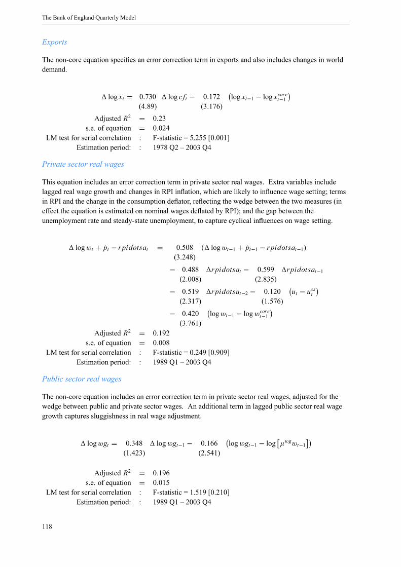
The Bank of England Quarterly Model
Exports
The non-core equation specifies an error correction term in exports and also includes changes in worlddemand.
log xt = 0.730(4.89)
log c ft − 0.172(3.176)
log xt−1 − log xcoret−1
Adjusted R2 = 0.23s.e. of equation = 0.024
LM test for serial correlation : F-statistic = 5.255 [0.001]Estimation period: : 1978 Q2 – 2003 Q4
Private sector real wages
This equation includes an error correction term in private sector real wages. Extra variables includelagged real wage growth and changes in RPI inflation, which are likely to influence wage setting; termsin RPI and the change in the consumption deflator, reflecting the wedge between the two measures (ineffect the equation is estimated on nominal wages deflated by RPI); and the gap between theunemployment rate and steady-state unemployment, to capture cyclical influences on wage setting.
logwt + pt − rpidotsat = 0.508(3.248)
( logwt−1 + pt−1 − rpidotsat−1)
− 0.488(2.008)
rpidotsat − 0.599(2.835)
rpidotsat−1
− 0.519(2.317)
rpidotsat−2 − 0.120(1.576)
ut − usst
− 0.420(3.761)
logwt−1 − logwcoret−1
Adjusted R2 = 0.192s.e. of equation = 0.008
LM test for serial correlation : F-statistic = 0.249 [0.909]Estimation period: : 1989 Q1 – 2003 Q4
Public sector real wages
The non-core equation includes an error correction term in private sector real wages, adjusted for thewedge between public and private sector wages. An additional term in lagged public sector real wagegrowth captures sluggishness in real wage adjustment.
logwgt = 0.348(1.423)
logwgt−1 − 0.166(2.541)
logwgt−1 − log µwgwt−1
Adjusted R2 = 0.196s.e. of equation = 0.015
LM test for serial correlation : F-statistic = 1.519 [0.210]Estimation period: : 1989 Q1 – 2003 Q4
118
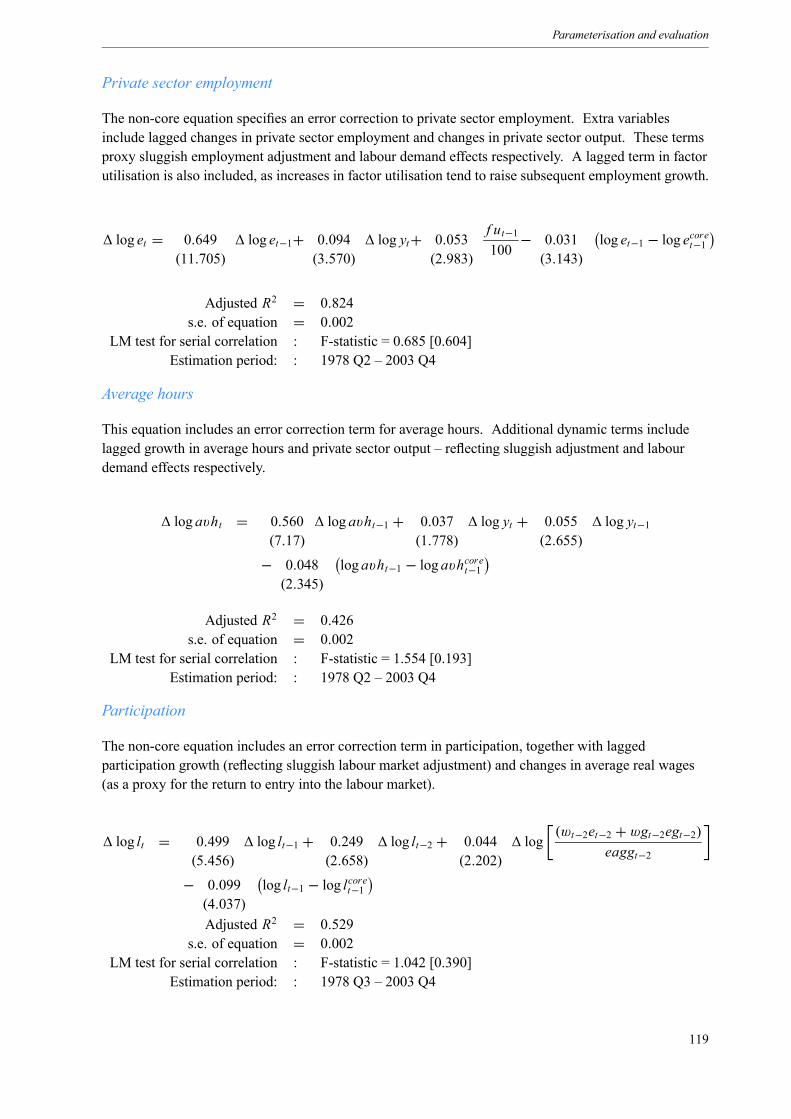
Parameterisation and evaluation
Private sector employment
The non-core equation specifies an error correction to private sector employment. Extra variablesinclude lagged changes in private sector employment and changes in private sector output. These termsproxy sluggish employment adjustment and labour demand effects respectively. A lagged term in factorutilisation is also included, as increases in factor utilisation tend to raise subsequent employment growth.
log et = 0.649(11.705)
log et−1+ 0.094(3.570)
log yt+ 0.053(2.983)
f ut−1100
− 0.031(3.143)
log et−1 − log ecoret−1
Adjusted R2 = 0.824s.e. of equation = 0.002
LM test for serial correlation : F-statistic = 0.685 [0.604]Estimation period: : 1978 Q2 – 2003 Q4
Average hours
This equation includes an error correction term for average hours. Additional dynamic terms includelagged growth in average hours and private sector output – reflecting sluggish adjustment and labourdemand effects respectively.
log avht = 0.560(7.17)
log avht−1 + 0.037(1.778)
log yt + 0.055(2.655)
log yt−1
− 0.048(2.345)
log avht−1 − log avhcoret−1
Adjusted R2 = 0.426s.e. of equation = 0.002
LM test for serial correlation : F-statistic = 1.554 [0.193]Estimation period: : 1978 Q2 – 2003 Q4
Participation
The non-core equation includes an error correction term in participation, together with laggedparticipation growth (reflecting sluggish labour market adjustment) and changes in average real wages(as a proxy for the return to entry into the labour market).
log lt = 0.499(5.456)
log lt−1 + 0.249(2.658)
log lt−2 + 0.044(2.202)
log(wt−2et−2 +wgt−2egt−2)
eaggt−2
− 0.099(4.037)
log lt−1 − log lcoret−1
Adjusted R2 = 0.529s.e. of equation = 0.002
LM test for serial correlation : F-statistic = 1.042 [0.390]Estimation period: : 1978 Q3 – 2003 Q4
119
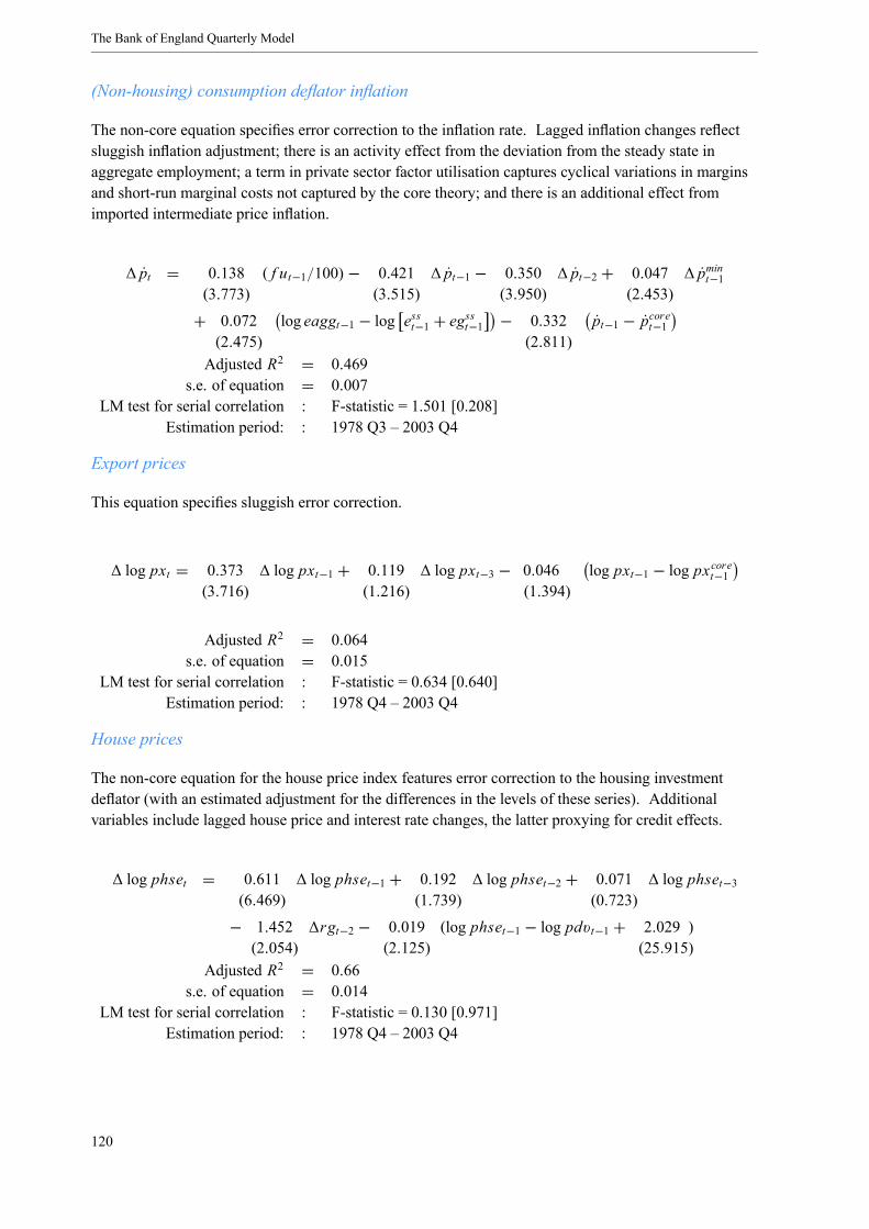
The Bank of England Quarterly Model
(Non-housing) consumption deflator inflation
The non-core equation specifies error correction to the inflation rate. Lagged inflation changes reflectsluggish inflation adjustment; there is an activity effect from the deviation from the steady state inaggregate employment; a term in private sector factor utilisation captures cyclical variations in marginsand short-run marginal costs not captured by the core theory; and there is an additional effect fromimported intermediate price inflation.
pt = 0.138(3.773)
( f ut−1/100)− 0.421(3.515)
pt−1 − 0.350(3.950)
pt−2 + 0.047(2.453)
pmint−1
+ 0.072(2.475)
log eaggt−1 − log esst−1 + egsst−1 − 0.332(2.811)
pt−1 − pcoret−1
Adjusted R2 = 0.469s.e. of equation = 0.007
LM test for serial correlation : F-statistic = 1.501 [0.208]Estimation period: : 1978 Q3 – 2003 Q4
Export prices
This equation specifies sluggish error correction.
log pxt = 0.373(3.716)
log pxt−1 + 0.119(1.216)
log pxt−3 − 0.046(1.394)
log pxt−1 − log pxcoret−1
Adjusted R2 = 0.064s.e. of equation = 0.015
LM test for serial correlation : F-statistic = 0.634 [0.640]Estimation period: : 1978 Q4 – 2003 Q4
House prices
The non-core equation for the house price index features error correction to the housing investmentdeflator (with an estimated adjustment for the differences in the levels of these series). Additionalvariables include lagged house price and interest rate changes, the latter proxying for credit effects.
log phset = 0.611(6.469)
log phset−1 + 0.192(1.739)
log phset−2 + 0.071(0.723)
log phset−3
− 1.452(2.054)
rgt−2 − 0.019(2.125)
(log phset−1 − log pdvt−1 + 2.029 )(25.915)
Adjusted R2 = 0.66s.e. of equation = 0.014
LM test for serial correlation : F-statistic = 0.130 [0.971]Estimation period: : 1978 Q4 – 2003 Q4
120

Parameterisation and evaluation
6.5 An evaluation of the model’s forecast performance
As discussed in Section 6.4.1, the simultaneity of the model means that its empirical fit should beevaluated as a system, rather than on a single-equation basis. In particular, a collection of equations thatappear to fit well for known values of the right-hand-side variables may not perform well whencombined to produce out-of-sample forecasts. Given that we wanted BEQM to fit the data at least aswell as the previous model, a natural test is to compare the properties of forecasts from BEQM and fromthe MTMM
We place less emphasis, therefore, on single equation properties than on how the equations worktogether as a system. The alternative approach of an equation-by-equation comparison of the non-coreequations with corresponding MTMM equations would be of limited use in any case, because theequations are not estimated conditional on the same information.
Method
We evaluate the forecasting performances of the MTMM and BEQM by running the two models assystems over history and measuring the prediction errors for a set of key endogenous variables. In doingso, we are in effect testing the performance of the models under something approaching actual forecastconditions. The main – and important – difference between what has been done here and actualforecasts is the application of judgement: the projections in this exercise have no judgementaladjustment, other than the routine residual adjustments required to enforce identities in the MTMM.Hence, the size of the forecast errors is likely to be substantially bigger than actual forecast errors.
We started the assessment by forecasting with each model at 1992 Q2, and recording the full paths forthe model’s projections of key endogenous variables over 13 quarters. We then moved one quarterahead to 1992 Q3 and repeated the exercise, allowing the models to ‘see’ actual outturns at 1992 Q2,rather than starting the new projection with the previous projection’s forecast values. This preventederrors in early projections from building up over time. We then repeated for each subsequent period toproduce a sequence of forecasts for each forecast horizon. Once the series of in-sample forecasts wasfinished, we analysed the prediction errors of the two models.
Some variables do not have well defined behavioural equations in the MTMM, including: nominalinterest rates, the nominal exchange rate, nominal government spending and the value of equities. Toensure comparability, we conditioned the MTMM projections on the paths for these variables generatedby BEQM.
The model versions
The exercise described above used the versions of the model that were current in the first half of 2003.This was to ensure a fair comparison, because the MTMM was not fully rebuilt and re-estimated to takeaccount of the shift to chain-weighted data in October 2003, so it would not be expected to perform aswell against more recent data. The in-sample period therefore runs from 1992 Q2 to 1999 Q3. It isconstrained at the beginning by the number of lags in the MTMM and the lack of comparable data forearlier periods, and at the end because we assessed forecasts up to 13 periods ahead.
121
The Bank of England Quarterly Model
Outputs
We focus on a subset of key variables: inflation (defined as the four-quarter growth rate of the RPIXindex), (69) the level of unemployment (the rate as defined in the Labour Force Survey) and thefour-quarter growth rates of GDP (at market prices), consumption, business investment, exports,imports, unit labour costs, and import prices (the import price deflator).
Prediction errors for inflation and unemployment rates are the percentage point difference of the actualand projected rates in each individual forecast; other prediction errors are measured as percentage pointdifferences of actual and projected four-quarter growth rates. From these errors, we can calculate avariety of statistical measures, such as Root Mean Squared Errors, Mean Absolute Errors and meanerrors. Information on the nature of the errors can be gained by decomposing squared prediction errorsinto bias, variance and covariance contributions. (70) We used Theil’s inequality coefficient to describehow good the forecasts are on an absolute scale. (71) And we used the Diebold-Mariano (1995)statistic (72) to test whether forecasts were significantly different from each other.
Results
The bar charts in Figure 6.4 summarise the relative forecasting performance of the two models overhistory. For each variable at a specified forecast horizon, the bar shows the root mean squared forecasterror from the MTMM less that from BEQM. A result of zero therefore indicates that the models haveidentical forecasting performance. The scale is in percentage point differences, so that a result of +1%means that the MTMM had a 1 percentage point higher root mean squared error than BEQM inforecasting that variable at that horizon. The results were mixed across variables and forecast horizons.But in general, BEQM tended to have a slightly lower forecast error at the two- and three-yearhorizon. (73)
Nevertheless, these differences were not great. Formal tests of whether the forecast errors aresignificantly different from each other suggest that the difference was not statistically significant for themajority of the variables at the five- and nine-quarter horizons. BEQM was significantly better forunemployment at both horizons, while worse for GDP growth at the nine-quarter horizon; for theremainder, there was no statistically significant difference. Overall, these results suggest that BEQMhas a ‘hands free’ forecasting performance that is at least as good as that of the MTMM.(74)
(69)The inflation target in the first half of 2003, when the exercise reported here was undertaken, was still set in terms of RPIX.(70)The mean of squared prediction errors can be decomposed into bias, variance and covariance:
1T
T
t=1yst − yat 2 = yst − yat
2 + σ s − σa 2 + 2 (1− ρ) σ sσa
where yst , yat , σ s , and σa are the means and standard deviations of the series ys (simulated or predicted series) and ya (actualdata) respectively, and ρ is their correlation coefficient.(71)See pages 30-37 of Theil (1961). The statistic computed here is Theil’s ‘U1’ measure. Comparisons using this statisticcontain more information than comparisons of root mean squared errors, since the U1 measure also accounts for differences inthe variability of predicted outcomes.(72)This procedure is designed to test the null of equal predictive ability between two models by considering the mean of thedifferences of squared prediction errors of the two competing models. We used a small-sample correction of this test statistic,proposed by Harvey, Leybourne and Newbold (1997).(73)A similar picture also holds if we consider the mean absolute and simple mean errors, not shown here.(74)This was an important part of the remit for developing BEQM as discussed in Section 2.1.
122
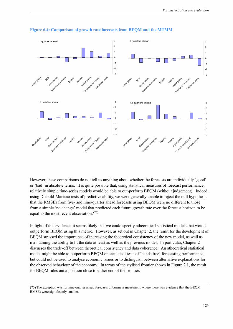
Parameterisation and evaluation
Figure 6.4: Comparison of growth rate forecasts from BEQM and the MTMM
9 quarters ahead
-3
-2
-1
0
1
2
3
Retail p
rices
GDP
Consu
mption
Busine
ss in
vestm
ent
Export
s
Impo
rts
Impo
rt pric
es
Unemplo
ymen
t (rate
)
Unit la
bour
costs
5 quarters ahead
-3
-2
-1
0
1
2
3
Retail p
rices
GDP
Consu
mption
Busine
ss in
vestm
ent
Export
s
Impo
rts
Impo
rt pric
es
Unemplo
ymen
t (rate
)
Unit la
bour
costs
1 quarter ahead
-3
-2
-1
0
1
2
3
Retail p
rices
GDP
Consu
mption
Busine
ss in
vestm
ent
Export
s
Impo
rts
Impo
rt pric
es
Unemplo
ymen
t (rate
)
Unit la
bour
costs
13 quarters ahead
-3
-2
-1
0
1
2
3
Retail p
rices
GDP
Consu
mption
Busine
ss in
vestm
ent
Export
s
Impo
rts
Impo
rt pric
es
Unemplo
ymen
t (rate
)
Unit la
bour
costs
However, these comparisons do not tell us anything about whether the forecasts are individually ‘good’or ‘bad’ in absolute terms. It is quite possible that, using statistical measures of forecast performance,relatively simple time-series models would be able to out-perform BEQM (without judgement). Indeed,using Diebold-Mariano tests of predictive ability, we were generally unable to reject the null hypothesisthat the RMSEs from five- and nine-quarter ahead forecasts using BEQM were no different to thosefrom a simple ‘no change’ model that predicted each future growth rate over the forecast horizon to beequal to the most recent observation. (75)
In light of this evidence, it seems likely that we could specify atheoretical statistical models that wouldoutperform BEQM using this metric. However, as set out in Chapter 2, the remit for the development ofBEQM stressed the importance of increasing the theoretical consistency of the new model, as well asmaintaining the ability to fit the data at least as well as the previous model. In particular, Chapter 2discusses the trade-off between theoretical consistency and data coherence. An atheoretical statisticalmodel might be able to outperform BEQM on statistical tests of ‘hands free’ forecasting performance,but could not be used to analyse economic issues or to distinguish between alternative explanations forthe observed behaviour of the economy. In terms of the stylised frontier shown in Figure 2.1, the remitfor BEQM rules out a position close to either end of the frontier.
(75)The exception was for nine quarter ahead forecasts of business investment, where there was evidence that the BEQMRMSEs were significantly smaller.
123
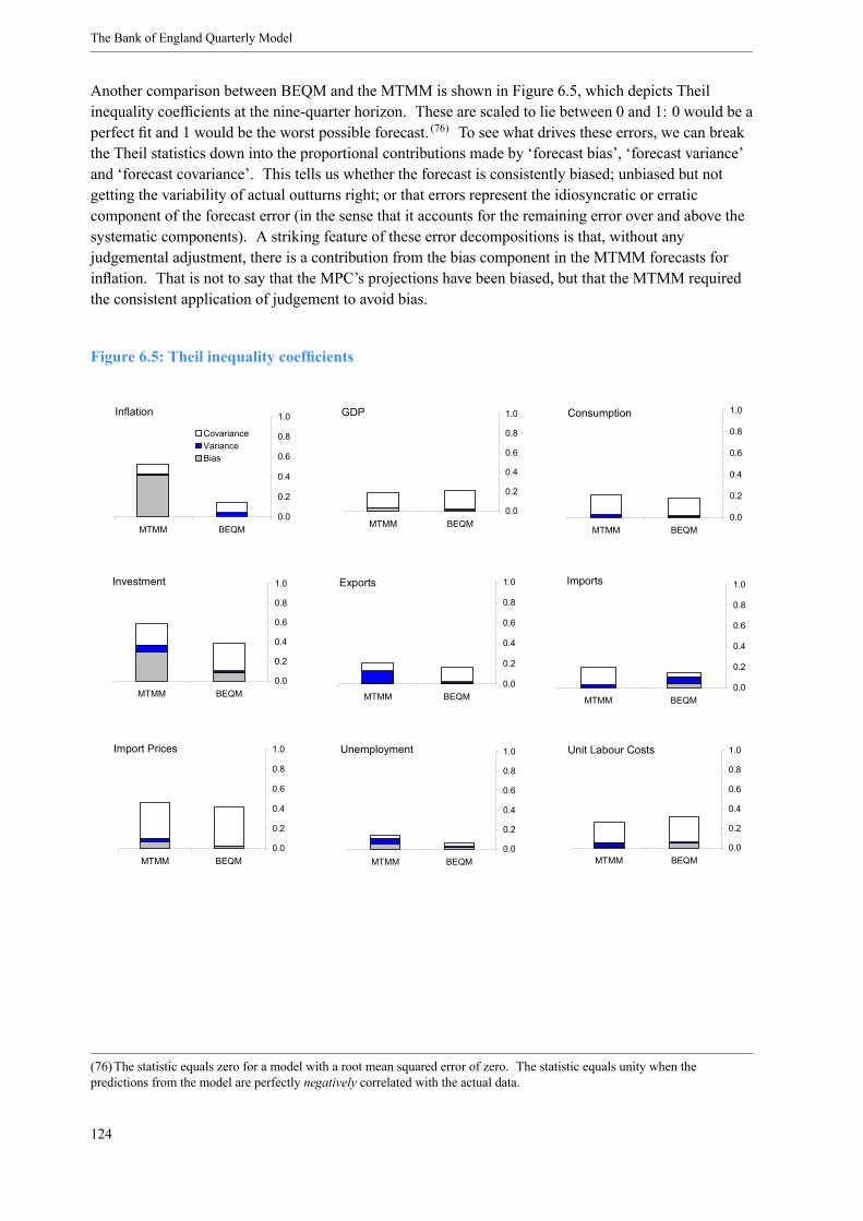
The Bank of England Quarterly Model
Another comparison between BEQM and the MTMM is shown in Figure 6.5, which depicts Theilinequality coefficients at the nine-quarter horizon. These are scaled to lie between 0 and 1: 0 would be aperfect fit and 1 would be the worst possible forecast. (76) To see what drives these errors, we can breakthe Theil statistics down into the proportional contributions made by ‘forecast bias’, ‘forecast variance’and ‘forecast covariance’. This tells us whether the forecast is consistently biased; unbiased but notgetting the variability of actual outturns right; or that errors represent the idiosyncratic or erraticcomponent of the forecast error (in the sense that it accounts for the remaining error over and above thesystematic components). A striking feature of these error decompositions is that, without anyjudgemental adjustment, there is a contribution from the bias component in the MTMM forecasts forinflation. That is not to say that the MPC’s projections have been biased, but that the MTMM requiredthe consistent application of judgement to avoid bias.
Figure 6.5: Theil inequality coefficients
Inflation
0.0
0.2
0.4
0.6
0.8
1.0
MTMM BEQM
CovarianceVarianceBias
GDP
0.0
0.2
0.4
0.6
0.8
1.0
MTMM BEQM
Consumption
0.0
0.2
0.4
0.6
0.8
1.0
MTMM BEQM
Investment
0.0
0.2
0.4
0.6
0.8
1.0
MTMM BEQM
Unit Labour Costs
0.0
0.2
0.4
0.6
0.8
1.0
MTMM BEQM
Unemployment
0.0
0.2
0.4
0.6
0.8
1.0
MTMM BEQM
Exports
0.0
0.2
0.4
0.6
0.8
1.0
MTMM BEQM
Imports
0.0
0.2
0.4
0.6
0.8
1.0
MTMM BEQM
Import Prices
0.0
0.2
0.4
0.6
0.8
1.0
MTMM BEQM
(76)The statistic equals zero for a model with a root mean squared error of zero. The statistic equals unity when thepredictions from the model are perfectly negatively correlated with the actual data.
124
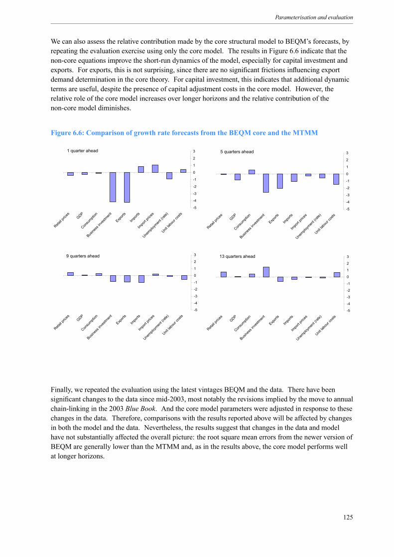
Parameterisation and evaluation
We can also assess the relative contribution made by the core structural model to BEQM’s forecasts, byrepeating the evaluation exercise using only the core model. The results in Figure 6.6 indicate that thenon-core equations improve the short-run dynamics of the model, especially for capital investment andexports. For exports, this is not surprising, since there are no significant frictions influencing exportdemand determination in the core theory. For capital investment, this indicates that additional dynamicterms are useful, despite the presence of capital adjustment costs in the core model. However, therelative role of the core model increases over longer horizons and the relative contribution of thenon-core model diminishes.
Figure 6.6: Comparison of growth rate forecasts from the BEQM core and the MTMM
9 quarters ahead
-5
-4
-3
-2
-1
0
1
2
3
Retail p
rices
GDP
Consu
mption
Busine
ss in
vestm
ent
Export
s
Impo
rts
Impo
rt pric
es
Unemplo
ymen
t (rate
)
Unit la
bour
costs
5 quarters ahead
-5
-4
-3
-2
-1
0
1
2
3
Retail p
rices
GDP
Consu
mption
Busine
ss in
vestm
ent
Export
s
Impo
rts
Impo
rt pric
es
Unemplo
ymen
t (rate
)
Unit la
bour
costs
1 quarter ahead
-5
-4
-3
-2
-1
0
1
2
3
Retail p
rices
GDP
Consu
mption
Busine
ss in
vestm
ent
Export
s
Impo
rts
Impo
rt pric
es
Unemplo
ymen
t (rate
)
Unit la
bour
costs
13 quarters ahead
-5
-4
-3
-2
-1
0
1
2
3
Retail p
rices
GDP
Consu
mption
Busine
ss in
vestm
ent
Export
s
Impo
rts
Impo
rt pric
es
Unemplo
ymen
t (rate
)
Unit la
bour
costs
Finally, we repeated the evaluation using the latest vintages BEQM and the data. There have beensignificant changes to the data since mid-2003, most notably the revisions implied by the move to annualchain-linking in the 2003 Blue Book. And the core model parameters were adjusted in response to thesechanges in the data. Therefore, comparisons with the results reported above will be affected by changesin both the model and the data. Nevertheless, the results suggest that changes in the data and modelhave not substantially affected the overall picture: the root square mean errors from the newer version ofBEQM are generally lower than the MTMM and, as in the results above, the core model performs wellat longer horizons.
125

The Bank of England Quarterly Model
6.6 Summary
This chapter describes our approach to parameterising and evaluating BEQM against the data. A firststep was to create a database with the required characteristics. Variables need to be detrended by theappropriate growth rate so that the model can be written in stationary form. And some modification ofvariables is necessary to make a better match with the underlying economic concepts.
The combination of a large, simultaneous model with the assumption of model-consistent expectationsraises difficult issues for parameterisation. These make conventional systems estimation procedureshard to apply, given the relatively short time series that were available. We therefore split the coremodel parameters into three groups according to whether they affect the steady state, the dynamics, orboth. This allows us to calibrate the steady state first, using an approximately recursive approach andcalibrating separate parts of the model as relatively self-contained blocks. In some cases we aim tomatch recent observations rather than full sample averages, where there are apparent trends or regimeshift.
We adopt a largely informal approach to parameterising the dynamics of the core model: we judge the fitagainst historical data; in terms of the responses to marginal shocks; and relative to the estimation resultsfor non-core equations. We choose parameters that give desired properties, such as inertia in realvariables, gradual pass-through from import price changes, and an appropriate mix of output andinflation responses.
The non-core equations are estimated mainly with error correction to the relevant core model paths,which are derived using actual data for predetermined variables and assuming that expectations aregenerated using the ‘exogenous variables model’ discussed in Chapter 5.
We present a number of evaluations of the model’s performance against the data. The design andstructure of BEQM mean that it should be evaluated as a system, rather than on a single-equation basis.We compare prediction errors for a key set of endogenous variables from running comparable versionsof BEQM and the MTMM over the past. In general, the results suggest that BEQM has slightly lowerforecast errors at the two- and three-year horizons, but few of the differences are statistically significant.Further tests suggest that there is a greater contribution from bias to inflation forecasts in the MTMMthan in BEQM; and that the non-core equations improve the short-term dynamics of BEQM, althoughless so at longer horizons. Finally, we repeat the evaluation using the latest versions of both BEQM andthe data. This suggests that recent changes to the model and the data have not substantially altered theoverall performance of BEQM relative to the MTMM.
126

Chapter 7 Model properties
This chapter presents the results of a series of model simulations to illustrate the properties of BEQM.Section 7.1 sets out some introductory remarks on the nature of the simulations and interpretation of theresults, which are described in Section 7.2. Finally, Section 7.3 summarises.
7.1 Interpreting the responses
The shock responses shown in Section 7.2 are intended to highlight specific mechanisms of the model,and so we focus on a few stylised experiments. Several points are worth noting about the nature of theseresults.
First, we assume that the economy is at its long-run equilibrium when the shock hits. (1) This is adifferent type of exercise from forecasts, which can be thought of as showing how an economy that isaway from a sustainable long-run equilibrium could move towards such a position.
Second, we generally assume that the shocks are unanticipated, but once they occur they are recognisedimmediately and fully understood. In other words, there is no assumption of partial information orlearning (discussed in Chapter 5), apart from in the variant of the interest rate shock (shown in Figure7.2) that we use to illustrate the effect of changing assumptions about agents’ expectations.
Third, each shock represents an isolated change to a single exogenous variable, which helps clarity but isa simplification compared with most forecast issues or historical episodes, which often involvesimultaneous shocks to a number of exogenous variables. Moreover, in the simulations presented here,the rest of the world is assumed not to react in any way. For example, we shock (exogenous) worldprices and world demand (see Sections 7.2.4 and 7.2.5), but no other world variables are assumed tochange in the experiments presented here. In many cases, we would expect other variables to change ina well articulated story about economic shocks, depending on the ultimate source of the shock.
Fourth, policy assumptions are important. In the first shock – designed to illustrate the impact of interestrate changes – we shock monetary policy directly. But interest rates are an endogenous variable,typically moving in response to some change in the economy. This shock represents an erratic deviationfrom the normal policy reaction function, which is different from most policy changes.
The other simulations are run under the assumption that policy reacts immediately: we do not conditionon a particular path for short-term interest rates or fiscal variables. Differences in policy assumptionscan have a significant impact on the responses, so it is important to interpret the reactions to shocks inthe light of the policy reaction functions used in the simulations. Here, we assume that the monetaryauthority targets inflation using short-term nominal interest rates and a Taylor-type reaction function; (2)
and a lump-sum household tax adjusts to ensure fiscal solvency, given policy targets for governmentexpenditure, debt, transfers and other taxes.
(1) The model’s decision rules are written in levels. The curvature of the assumed utility, production and demand functionsimparts a mild non-linearity to the whole system. Shock responses therefore always depend on the starting point. Testing hasindicated that reasonable differences in the initial steady-state equilibria are unlikely to make a qualitative difference to theoverall response.(2) The version we use gives some weight to lagged interest rates. See Appendix A for full details of the reaction function weuse for these simulations.
127

The Bank of England Quarterly Model
Finally, it matters whether the shocks are permanent or temporary. As explained below, the interest rateshock used here is a temporary shock, so that the model can return to equilibrium. The other shocks areconfigured as permanent shocks, in order to show how the model moves from one steady-stateequilibrium to another. This has implications for behaviour, particularly through the behaviour ofagents’ expectations and asset prices. Shocks that are understood to be temporary tend to have smallereffects on asset prices, because there is no long-term movement in asset prices (unlike the results of thepermanent shocks discussed in Sections 7.2.2 to 7.2.6).
7.2 Shock responses
This section discusses the behaviour of the full model in the face of shocks to monetary policy,productivity, government spending, the terms of trade, world demand, and labour supply. We havechosen these shocks to illustrate the interactions of households, firms and policymakers in goods, labourand financial markets. The temporary monetary policy shock is described by the impact of the initialshock and how the economy returns to equilibrium. However, we find it more intuitive to describe theother, permanent shocks by starting with the determination of the new steady-state equilibrium, and thenthe short-run dynamics. Where possible, we discuss the responses in the light of the conclusions ofdirectly comparable empirical literature.
For each shock, we show a standard set of eight charts (using the same scales for each shock); for thepermanent shocks in Section 7.2.2 to Section 7.2.6 we show some additional detail to help illustrate theparticular effects. The new steady state in the permanent shocks is shown as a dashed line. All theshocks discussed in this chapter start with the economy at a steady-state equilibrium.
Some asset stocks, especially net foreign assets, are quite slow to get to their new steady-stateequilibrium positions in the face of most of the permanent shocks. So flows can be very close to theirlong-run equilibrium positions, but it may take some time before stocks reach equilibrium. In the case ofnet foreign assets, adjustment occurs through net trade and the short-run trade responses can be quitedifferent from the long-run balance required for a sustainable equilibrium. In general, the persistence ofexpenditures means that we often see short-term overshooting in net foreign assets. (3)
7.2.1 An interest rate shock
Figure 7.1 illustrates the effect of a 1 percentage point rise in nominal interest rates for four quarters. Itis designed to show the direct impact of interest rate changes on the model economy. In the othersimulations presented in this section, interest rates react endogenously to movements in inflation andoutput that come about because of some other shock. But here, we start with an interest rate movementand follow the reaction of the rest of the model. In particular, we assume that monetary policy can bedescribed by a simple Taylor-type reaction function in which nominal interest rates react to inflation andoutput gaps, and we fix the nominal interest rate by shocking the monetary policy reaction functiondirectly. (4)
(3) Eigenanalysis of the model confirms that it is stable, but the estimated dynamics imply that convergence is slow.(4) The mechanics of implementing the shock are described in Box 11 on page 80.
128

Model properties
Implemented this way, using the recursive simulation technique discussed in Chapter 5, the shock can bethought of as a sequence of unanticipated deviations from the monetary policy that would be expectedon the basis of private agents’ understanding of the economy and, in particular, the monetary policyreaction function. This is not the same as exogenising monetary policy by removing the monetaryreaction function. In each period, agents see interest rates that do not accord with their understandingabout how monetary policy is usually set; (5) they nonetheless expect monetary policy in subsequentperiods to be set according to the normal reaction function, and remain confident that inflation willremain anchored at the original target in the long run.
The responses to this shock reflect the theoretical structure of the model discussed in Chapter 3.Optimal decisions are made on the basis of relative prices, taking account of the general level of prices.This ensures long-run neutrality of monetary policy so that the only long-run change is that nominalprices all move by the same proportion. Relative prices are unaffected in the steady state, so there are nolong-run effects on real expenditures or the rate of inflation, which is brought back to target by themonetary reaction function.
But there are potentially significant effects in the short run. The model incorporates a number ofrigidities that reflect costly adjustment of prices and quantities. Broadly speaking, the balance of theserigidities determines the extent to which a monetary policy shock will affect inflation or real activity inthe short run. (6) For example, we assume that it is costly for firms to adjust their factor inputs andnominal prices. Firms balance the costs of adjusting factors of production and of adjusting prices, sothat the overall price/quantity response will depend on the relative costs of adjustment. There is avariety of other rigidities that also affect the overall output/inflation response. And there are additionalchannels of short-run ‘non-neutrality’ of monetary policy shocks. For example, changes in nominalinterest rates may affect real consumption growth in the short run, to the extent that they representchanges in the credit constraints faced by consumers.
Because nominal prices and wages are assumed to be sticky and inflation is assumed to be persistent, theincrease in the nominal interest rate leads to an increase in the real interest rate, and hence the cost ofborrowing to finance consumption and investment. The nominal exchange rate immediately appreciateswith the increase in nominal interest rates, in line with uncovered interest parity. (7) This has two effects.First, domestic price stickiness means that there is a real exchange rate appreciation, which reduces thedemand for exports. Second, the nominal appreciation puts downward pressure on import prices, whichfeeds through gradually because of price stickiness. Other things equal, this effect would increase thedemand for imports, but the income effect from lower demand dominates in the short run.
(5) Leeper and Zha (2003) make the distinction between the ‘direct’ effects of a policy intervention, which are the usualreactions when the regime is held fixed, and the ‘expectation-formation’ effects that are introduced by changes in agents’beliefs about the policy regime. In their language, the simulation shown in Figure 7.1 is assumed to be a ‘modest’ intervention,where there are no expectation-formation effects.(6) If all prices were completely flexible, then temporary monetary policy shocks would lead to an immediate change in allnominal prices, without any effect on real expenditure. The long-run effects of the shock would be observed immediately.(7) The exchange rate appreciation follows from the fact that higher domestic interest rates, relative to interest rates onequivalent foreign-currency assets, make sterling assets more attractive to international investors. Uncovered interest parityimplies that the exchange rate moves to a level where investors expect a future depreciation just large enough to make themindifferent between holding domestic and foreign-currency assets. When used for forecasting, alternative paths for the nominalexchange rate are typically used, as discussed in the box ‘The exchange rate in forecasting and policy analysis’ on page 48 ofthe November 1999 Inflation Report.
129
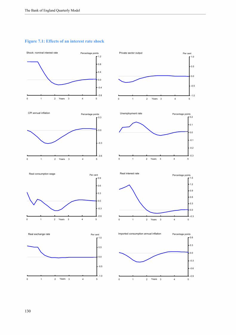
The Bank of England Quarterly Model
Figure 7.1: Effects of an interest rate shock
Private sector output
-1.0
-0.5
0.0
0.5
1.0
0 1 2 3 4 5Years
Per cent
CPI annual inflation
-0.6
-0.3
0.0
0.3
0 1 2 3 4 5Years
Percentage points Unemployment rate
-0.3
-0.2
-0.1
0.0
0.1
0.2
0 1 2 3 4 5Years
Percentage points
Real consumption wage
-0.6
-0.3
0.0
0.3
0.6
0.9
0 1 2 3 4 5Years
Per cent Real interest rate
-0.3
0.0
0.3
0.6
0.9
1.2
1.5
0 1 2 3 4 5Years
Percentage points
Real exchange rate
-1.0
-0.5
0.0
0.5
1.0
0 1 2 3 4 5Years
Per cent Imported consumption annual inflation
-0.9
-0.6
-0.3
0.0
0.3
0.6
0 1 2 3 4 5Years
Percentage points
Shock: nominal interest rate
-0.8
-0.4
0.0
0.4
0.8
1.2
0 1 2 3 4 5Years
Percentage points
130

Model properties
All of these effects act to reduce aggregate demand. In the face of unchanged potential supply, firmsimmediately reduce factor utilisation and start to reduce employment and investment. Though prices aresticky, they are not fixed and inflation falls below the starting rate as firms react to the fall in demand.Real consumption wages rise in the very first period, but fall back quickly as a result of lower demandfor labour. Fiscal policy reacts by increasing the lump sum tax rate to preserve tax revenue as nominalGDP falls in the short run.
The shock lasts for four periods. In the fifth period, monetary policy reverts to its standard reactionfunction. Faced with a negative output gap and inflation below target, nominal interest rates graduallyfall below their long-run equilibrium to bring inflation back to target. The economy is close toequilibrium after five years.
The responses shown here accord qualitatively with the broad conclusions from the empirical literatureon monetary policy shocks: following an unanticipated monetary policy tightening, interest rates rise,output contracts, profits and real wages fall, and inflation (eventually) falls. Output, consumption,investment and inflation are ‘hump-shaped’ and highly persistent, with the peak effect on inflationlagging the peak effect on real variables. (8) The behaviour of the model for this shock is broadly similarto that of the previous MTMM model (9) and qualitatively close to other studies of the UK economy. (10)
The simulation shown in Figure 7.1 is based on the assumption that the unexpected change in interestrates does not affect agents’ long-run inflation expectations. But the response of the economy to achange in interest rates depends on the credibility of the inflation target. In particular, as inflationexpectations become more firmly anchored around the inflation target – the target becomes morecredible – a change in the short-term interest rate is likely to have less impact.
To illustrate the sensitivity of these simulations to assumptions about expectations, Figure 7.2 showshow the effect on inflation and private sector output differs if agents wrongly perceive that theunexpected increase in interest rates may have been triggered by a reduction in the targeted rate ofinflation. The blue line is the same as in Figure 7.1 and the black line is based on the assumption thatagents revise down their expectation of the targeted rate of inflation and expect a prolonged period oftighter policy in order to achieve that perceived lower target. (11)
(8) See, for example, Leeper, Sims and Zha (1996), Leeper and Zha (2003) and Christiano, Eichenbaum and Evans (1997,1999).(9) See Bank of England (2004).(10)See, for example, Batini, Harrison and Millard (2003), Bean, Larsen and Nikolov (2002) and Dale and Haldane (1995). Inmany of these studies, the responses are very persistent – more than we judge to be plausible. Bean (1998) estimates an IScurve and Phillips curve instead of a VAR; in that model output drops immediately and there is no effect on inflation for oneyear. But the signs and ordering of output and inflation responses in these studies are otherwise the same.(11)This simulation is sensitive to the precise assumptions made about the change in expected inflation. Here we assume thatthe unexpected increase in interest rates causes agents to revise down their expected level of inflation in the long run by around0.2 percentage points by the end of the first year.
131
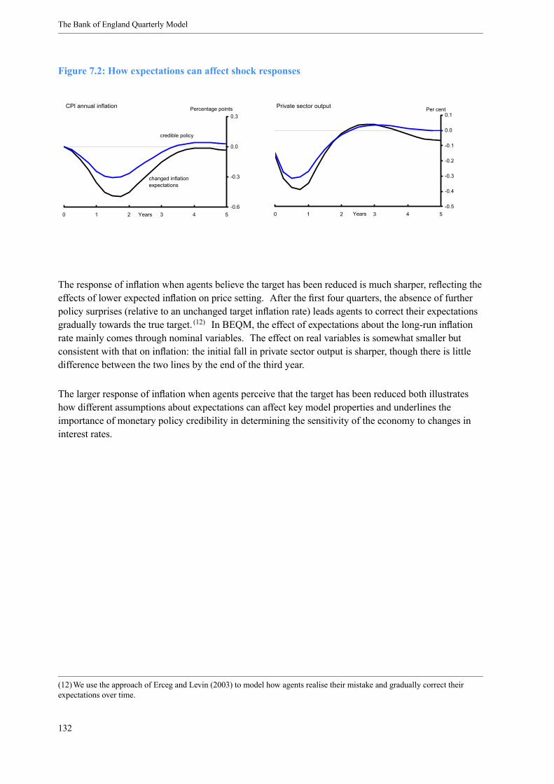
The Bank of England Quarterly Model
Figure 7.2: How expectations can affect shock responses
Private sector output
-0.5
-0.4
-0.3
-0.2
-0.1
0.0
0.1
0 1 2 3 4 5Years
Per centCPI annual inflation
-0.6
-0.3
0.0
0.3
0 1 2 3 4 5Years
Percentage points
changed inflationexpectations
credible policy
The response of inflation when agents believe the target has been reduced is much sharper, reflecting theeffects of lower expected inflation on price setting. After the first four quarters, the absence of furtherpolicy surprises (relative to an unchanged target inflation rate) leads agents to correct their expectationsgradually towards the true target. (12) In BEQM, the effect of expectations about the long-run inflationrate mainly comes through nominal variables. The effect on real variables is somewhat smaller butconsistent with that on inflation: the initial fall in private sector output is sharper, though there is littledifference between the two lines by the end of the third year.
The larger response of inflation when agents perceive that the target has been reduced both illustrateshow different assumptions about expectations can affect key model properties and underlines theimportance of monetary policy credibility in determining the sensitivity of the economy to changes ininterest rates.
(12)We use the approach of Erceg and Levin (2003) to model how agents realise their mistake and gradually correct theirexpectations over time.
132
Model properties
7.2.2 A productivity shock
Figure 7.3 shows the effects of a permanent 1% increase in the level of labour productivity. (13) Thissimulation is of particular interest because it highlights the importance of stock-flow dynamics and thewealth dimension of the model, and illustrates how demand and policy react to supply shifts.
In the long run, with the new steady-state shown by the dashed line in Figure 7.3, the increase in labourproductivity is accompanied by a rise in wages paid by firms. Desired capital and potential supply alsoincrease (although proportionately less than the size of the productivity shock, due to the second roundeffects on supply discussed below).
Households increase their consumption, given higher wages. Aggregate import levels rise with theincrease in consumption and capital investment. The economy must export more to restore externalbalance, and a real exchange rate depreciation is required. Steady-state external balance is brought aboutby an increase in the trade surplus (or reduction in deficit), offset by a fall in net foreign asset levels. (14)
We could also tell this story equivalently in terms of stocks. The increase in productivity raises thelong-run value of equities (15) and corporate debt; and government debt rises broadly in line with output.Some of the increase in domestic financial assets is sold to overseas residents, which results in adecrease in net foreign assets. An increase in net exports is needed to service the extra debt and so thereal exchange rate depreciates.
This depreciation has two ‘second-round’ effects on the real economy, through labour supply andcapital, which reduce the overall impact on long-run supply.
First, we make a distinction in BEQM between real consumer wages and real producer wages. Thelong-run real consumption wage rises unambiguously, but by less than the real producer wage, becausethe exchange rate depreciation causes an increase in total consumption prices (including importedgoods) relative to domestic producer prices. At the same time, the reservation wage rises fully in linewith the increase in labour productivity. (16) The combined effect is sufficient to cause a small long-runfall in labour supply and employment, which mitigates the output increase from the productivity shock.
Second, the long-run price of imported goods rises relative to domestically produced goods. Thisreduces slightly the ratios of imported to domestically produced consumption and capital goods, butimports of capital goods still rise in absolute terms. (17) This relative price effect raises the overall costof capital goods, which also offsets part of the increase in capital and output from the productivityshock. (18)
(13) It is implemented as a 1 percentage point increase in the growth rate of labour productivity for one period.(14)Figure 7.1 shows that there is little change in the steady-state ratio of net foreign assets to GDP. The initial equilibrium hasa negative level of net foreign assets. It is the combination of a fall in the level of net foreign assets (thus becoming morenegative) and a rise in GDP that leaves the steady-state ratio of the two virtually unchanged.(15)The long-run value of the firm is equal to the value of the capital stock plus the expected stream of discounted supernormalprofits. The value of equity increases by slightly less than the value of the capital stock because the exchange rate depreciationmeans that value-added prices fall relative to consumer prices. This reduces real average profitability in terms of consumerprices.(16)We assume that unemployment benefits move in line with the real product wage, and hence labour productivity. This is anecessary assumption to prevent the long-run natural rate of unemployment trending above 100% or below zero in the long run.(17) Imported and domestically produced capital goods are assumed to be complements.(18)The amount of the increase in the desired capital stock depends on the share of imported capital in the capital aggregator,the elasticity of substitution between imported and domestic capital goods, and the elasticity of export demand.
133
The Bank of England Quarterly Model
The exchange rate movement is associated with some permanent shifts in relative prices, but inflationand nominal interest rates return to the initial equilibrium implied by the inflation target and worldnominal interest rates, leaving the real interest rate unchanged. There is little fiscal policy reaction:government transfers spending and debt are all assumed to rise in line with output, and tax revenues risebroadly in line with output too. (19)
In the long run, therefore, there is no change in the inflation rate and nominal interest rates, with anoverall increase in output flows. The economy exports more and holds more foreign debt, with adepreciation in the real exchange rate. The fact that output does not rise by exactly 1% is due to thesecond-round impacts of the real exchange rate on desired labour supply and capital.
Turning to the short run, firms are immediately able to produce more output, for given inputs of capitaland labour. But sluggish adjustment means that aggregate demand does not immediately increase and sofactor utilisation falls sharply. This encourages firms both to reduce prices to stimulate demand and toreduce their demand for labour in the short run. The real exchange rate immediately depreciates close toits new long-run level and this is gradually passed through into higher import price inflation. Consumerprice inflation falls because the effect of temporarily reduced domestic prices outweighs the effect ofhigher import prices. Unemployment rises in the short run, as firms begin to reduce employment inresponse to the fall in factor utilisation. The fall in employment (and rise in unemployment) is relativelyshort lived, however, as higher real wages mean that demand rises steadily, bringing utilisation back tonormal levels. Monetary policy responds to low inflation and output below potential by cutting interestrates to stimulate demand. This prevents inflation from falling further, and the inflation rate graduallyrises back towards the target.
There is a large body of empirical literature that aims to identify the responses to a productivity shock.The responses here are consistent with the findings from that literature: investment, consumption andoutput all increase. (20) However, there is some disagreement over labour market responses, especiallywhether hours worked rise or fall. (21) The responses here are also consistent with the initial responsesfrom the MTMM model: output rises gradually to a higher level, and inflation falls quickly before risingback to its starting point. Work applying the methods of Bayoumi and Eichengreen (1992) andMonticelli and Tristani (1999) to UK data also corroborates this finding in the data.
(19)Real lump-sum taxes do not move by exactly the same amount as real domestic output, because the government spendingand debt targets are expressed in terms of ratios to the value of private sector output, and the GDP deflator changes a littlebecause of the permanent effects on the real exchange rate.(20)See, for example, Christiano, Eichenbaum and Evans (2001).(21) In a widely cited paper, Galí (1999) reports that hours worked fall after a positive productivity shock. Several studies haveaffirmed this proposition – see, for example, Basu, Fernald and Kimball (1998). But Christiano, Eichenbaum and Vigfusson(2003) argue that hours worked rise, consistent with the neoclassical model.
134
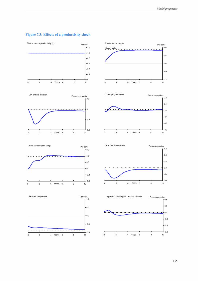
Model properties
Figure 7.3: Effects of a productivity shock
Private sector output
-1.0
-0.5
0.0
0.5
1.0
0 2 4 6 8 10Years
Per cent
Steady state
CPI annual inflation
-0.6
-0.3
0
0.3
0 2 4 6 8 10Years
Percentage pointsUnemployment rate
-0.3
-0.2
-0.1
0.0
0.1
0.2
0 2 4 6 8 10Years
Percentage points
Real consumption wage
-0.6
-0.3
0.0
0.3
0.6
0.9
0 2 4 6 8 10Years
Per centNominal interest rate
-0.8
-0.4
0.0
0.4
0.8
1.2
0 2 4 6 8 10Years
Percentage points
Real exchange rate
-1.0
-0.5
0.0
0.5
1.0
0 2 4 6 8 10Years
Per cent Imported consumption annual inflation
-0.9
-0.6
-0.3
0.0
0.3
0.6
0 2 4 6 8 10Years
Percentage points
Shock: labour productivity (λ)
0.0
0.2
0.4
0.6
0.8
1.0
1.2
0 2 4 6 8 10Years
Per cent
135
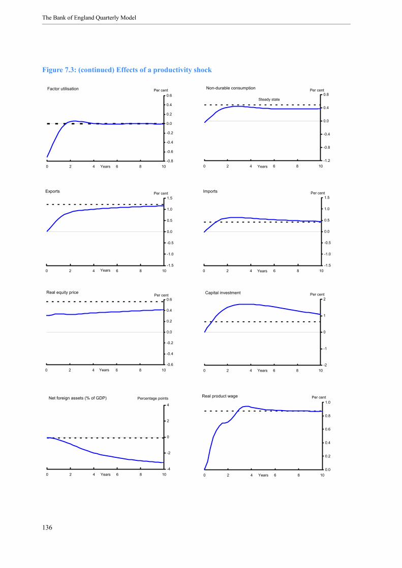
The Bank of England Quarterly Model
Figure 7.3: (continued) Effects of a productivity shock
Real product wage
0.0
0.2
0.4
0.6
0.8
1.0
0 2 4 6 8 10Years
Per cent
Capital investment
-2
-1
0
1
2
0 2 4 6 8 10Years
Per cent
Non-durable consumption
-1.2
-0.8
-0.4
0.0
0.4
0.8
0 2 4 6 8 10Years
Per cent
Steady state
Exports
-1.5
-1.0
-0.5
0.0
0.5
1.0
1.5
0 2 4 6 8 10Years
Per cent
Real equity price
-0.6
-0.4
-0.2
0.0
0.2
0.4
0.6
0 2 4 6 8 10Years
Per cent
Net foreign assets (% of GDP)
-4
-2
0
2
4
0 2 4 6 8 10Years
Percentage points
Factor utilisation
-0.8
-0.6
-0.4
-0.2
0.0
0.2
0.4
0.6
0 2 4 6 8 10Years
Per cent
Imports
-1.5
-1.0
-0.5
0.0
0.5
1.0
1.5
0 2 4 6 8 10Years
Per cent
136

Model properties
7.2.3 A government spending shock
Figure 7.4 illustrates the effect of a 5% increase in the (exogenous) target level of government spendingon private sector goods and services, defined as a ratio of nominal government spending to nominalprivate sector output. (22) The fiscal instrument – here, for simplicity, modelled as the lump-sum tax onhouseholds – then ensures that this new spending target is sustainable. This simulation is particularlyinteresting because of the shock’s direct effect on demand.
In the long run, the model shows conventional crowding-out effects, with reduced consumption becausetaxes must rise to pay for higher government spending. The higher lump-sum taxes cause households toreduce both non-durable consumption and dwellings investment.
In many textbook open economy models, output would be unchanged in the long run. (23) However,potential supply in BEQM can be affected (albeit only slightly in practice) by movements in the realexchange rate. The long-run change in the real exchange rate depends on the net impact of the shiftfrom private to public consumption on the long-run demand for imports. The import content of totalgovernment spending (including factor payments) is relatively low, but the intermediate importpropensity of government procurement is higher than that of domestically produced private non-durableconsumption. So the long-run demand for imports rises, but there is also a fall in direct imports ofconsumption goods that partially offsets this effect. Overall, the net effect is to increase slightly thelong-run demand for imports. As a result, the real exchange rate depreciates to raise exports andmaintain current account balance.
This depreciation has the same ‘second round’ effects as seen in the productivity shock, though theeffects here are quantitatively very small. First, increases in the price of imported consumption goodslower the real consumption wage and, hence, labour supply and employment. Second, increases in theprice of imported capital goods raise the overall cost of capital goods and lower the long-run level of thecapital stock. Output consequently falls slightly in the long run.
Despite a fall in the capital stock, the valuation of the corporate sector rises because of an increase in theprice of capital goods, which raises the overall (relative) value of the capital stock. (24) There is a slightrebalancing of portfolios – net foreign asset levels fall – but the effect is quantitatively small.
In the short run, government procurement increases immediately, but the crowding out of privateconsumption takes longer to come through. This reflects the non-Ricardian nature of the model (seeSection 3.2.1) and also the existence of habits. The net effect is an immediate rise in aggregate demandand factor utilisation. Higher factor utilisation stimulates the demand for labour (though moregradually) and encourages firms to increase margins. Domestic inflation rises as a result of the increasein factor costs and demand pressures. Imported inflation also rises somewhat due to the depreciation ofthe real exchange rate. The peak effect on CPI inflation occurs at around six quarters, reflecting nominalrigidities in domestic price setting and gradual pass through of the exchange rate to import prices.Monetary policy responds to the short-run increase in aggregate demand by raising the nominal interestrate to bring inflation back to target. After some time, the crowding-out effect on consumption also
(22)Government spending on private sector goods and services (‘procurement’) is only part of total government expenditure.The final increase in total government consumption, as measured by the National Accounts, is much less than 5%, becauseprocurement does not include wages and salaries paid to government employees or the government’s gross operating surplus.For this simulation, the government spending rule was modified to bring spending immediately up to the new target level.(23)The only net effect would be a reduction in the share of consumption in total expenditure.(24)There is also a technical effect that comes from our assumption of different mark-ups across expenditure categories as away of incorporating relative price trends with goods produced by a single production function (as explained in Section 6.3).
137

The Bank of England Quarterly Model
reduces aggregate demand, which fully adjusts within four years. Factor utilisation returns to normalbut unemployment adjusts more gradually because of rigidities in the labour market.
While there is increasing consensus on the responses of the economy to monetary policy and technologyshocks, there is less consensus on the effects of a fiscal policy shock. A major difficulty is in identifyingunanticipated shocks to fiscal policy, rather than systematic movements in spending through the businesscycle. Moreover, the responses are sensitive to whether an increase in government spending is expectedto be matched by higher future taxation or by lower future spending: changes in government spending inpractice could be associated with very different beliefs about what will happen in the future and when.So such simulations are not always a good guide to what happens in practice.
Nevertheless, the responses here are consistent with results from event studies of governmentprocurement: increases in government spending are associated with short-lived increases in privatesector output. (25) In some studies, evidence is found for short-run increases in consumption as well asinvestment. (26) In BEQM, private consumption falls immediately. (27) However, robust findings aredifficult to come by for the United Kingdom. (28) The trade balance immediately worsens, in line withRoubini (1988), but in general there is little agreement on the effect on the current account. (29) Atextbook result is that output is crowded out by higher public expenditure; this is seen here and in theMTMM model. But ‘crowding-in’ is a possibility in an open economy. (30)
(25)See Burnside, Eichenbaum and Fisher (BEF) (2002), following the methodology of Ramey and Shapiro (1998). Theresults in BEF indicate that real wages fall following an increase in government procurement. This is not the case here, asthere is a rise initially in real consumption wages.(26)See Blanchard and Perotti (2002).(27)This accords with the empirical findings reported in Cavallo (2002).(28)For example, Perotti (2002) finds that the short-run effects of government spending on inflation and output in five OECDeconomies (including the United Kingdom) has changed substantially over time.(29) In contrast to Roubini (1988), Roubini and Kim (2003) report that expansionary fiscal shocks tend to improve the currentaccount. See Erceg, Guerrieri and Gust (2004) for an assessment and discussion.(30)See Barry and Devereux (2003).
138
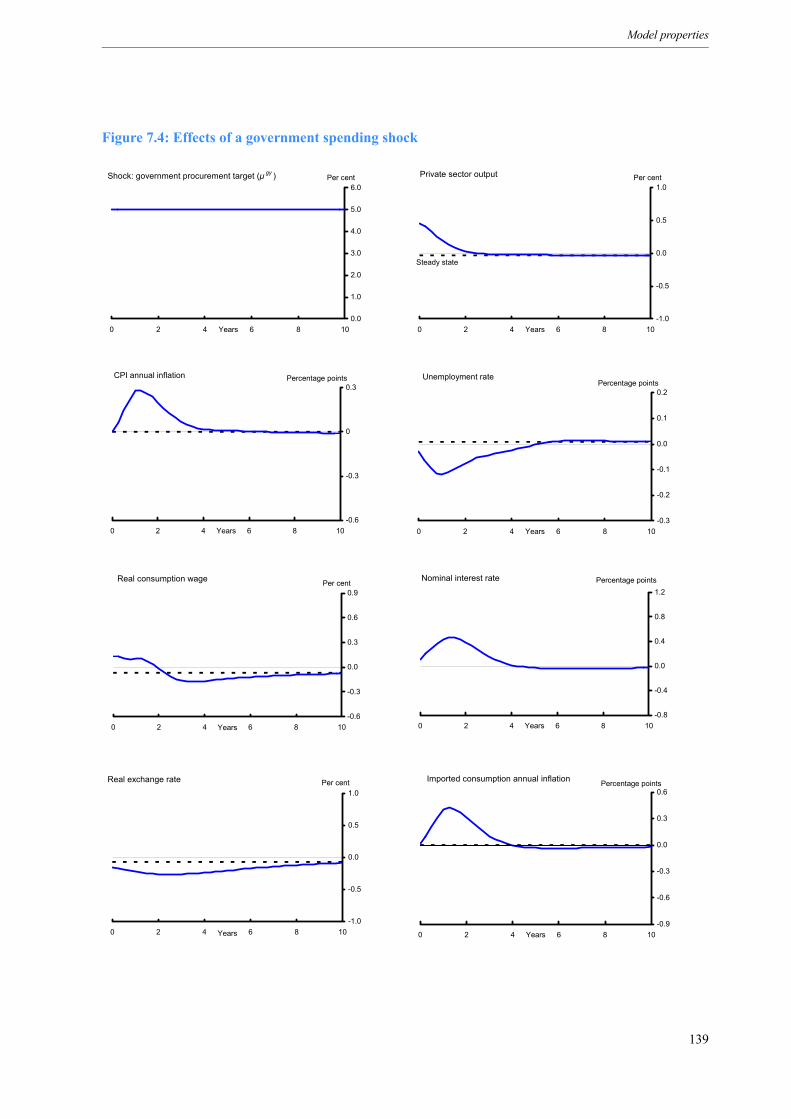
Model properties
Figure 7.4: Effects of a government spending shock
Private sector output
-1.0
-0.5
0.0
0.5
1.0
0 2 4 6 8 10Years
Per cent
Steady state
CPI annual inflation
-0.6
-0.3
0
0.3
0 2 4 6 8 10Years
Percentage points Unemployment rate
-0.3
-0.2
-0.1
0.0
0.1
0.2
0 2 4 6 8 10Years
Percentage points
Real consumption wage
-0.6
-0.3
0.0
0.3
0.6
0.9
0 2 4 6 8 10Years
Per cent Nominal interest rate
-0.8
-0.4
0.0
0.4
0.8
1.2
0 2 4 6 8 10Years
Percentage points
Real exchange rate
-1.0
-0.5
0.0
0.5
1.0
0 2 4 6 8 10Years
Per cent Imported consumption annual inflation
-0.9
-0.6
-0.3
0.0
0.3
0.6
0 2 4 6 8 10Years
Percentage points
Shock: government procurement target (µ gy )
0.0
1.0
2.0
3.0
4.0
5.0
6.0
0 2 4 6 8 10Years
Per cent
139
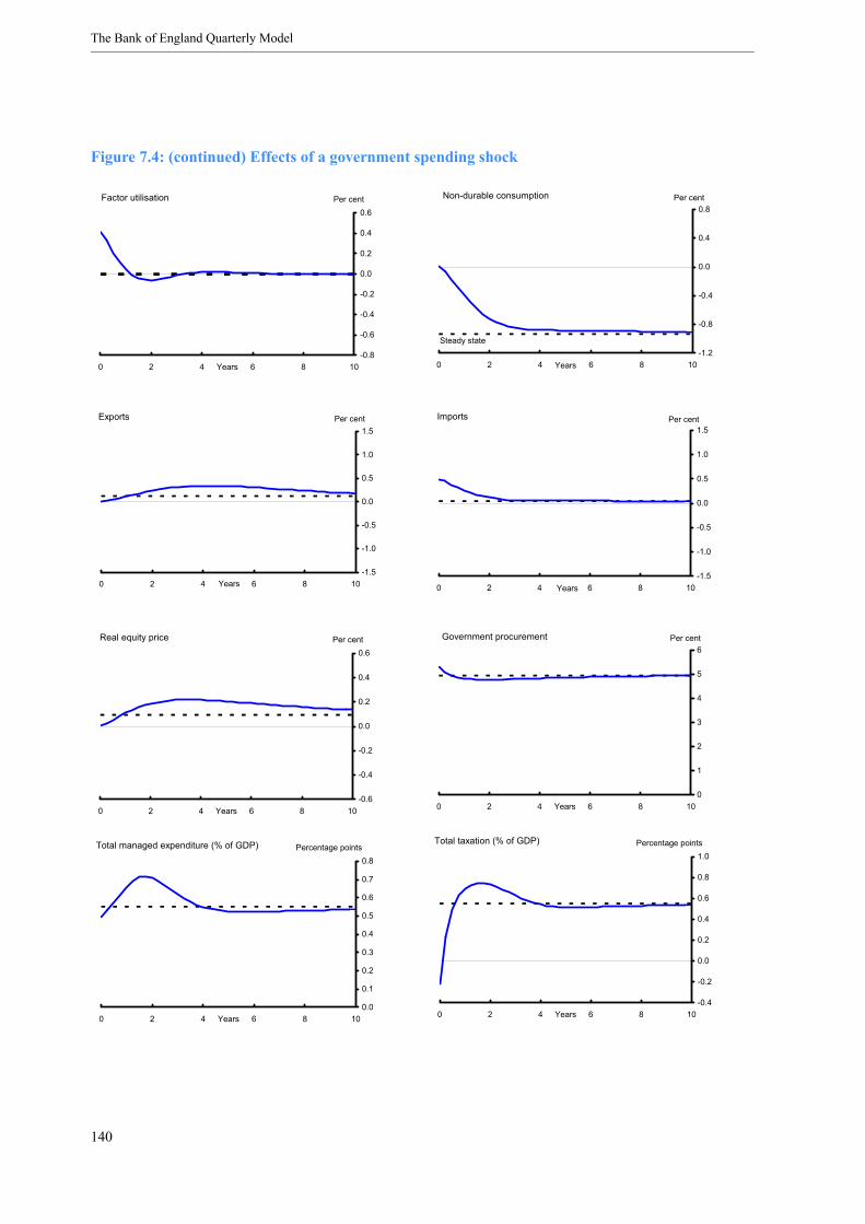
The Bank of England Quarterly Model
Figure 7.4: (continued) Effects of a government spending shock
Non-durable consumption
-1.2
-0.8
-0.4
0.0
0.4
0.8
0 2 4 6 8 10Years
Per cent
Steady state
Real equity price
-0.6
-0.4
-0.2
0.0
0.2
0.4
0.6
0 2 4 6 8 10Years
Per cent
Exports
-1.5
-1.0
-0.5
0.0
0.5
1.0
1.5
0 2 4 6 8 10Years
Per cent Imports
-1.5
-1.0
-0.5
0.0
0.5
1.0
1.5
0 2 4 6 8 10Years
Per cent
Government procurement
0
1
2
3
4
5
6
0 2 4 6 8 10Years
Per cent
Factor utilisation
-0.8
-0.6
-0.4
-0.2
0.0
0.2
0.4
0.6
0 2 4 6 8 10Years
Per cent
Total managed expenditure (% of GDP)
0.0
0.1
0.2
0.3
0.4
0.5
0.6
0.7
0.8
0 2 4 6 8 10Years
Percentage pointsTotal taxation (% of GDP)
-0.4
-0.2
0.0
0.2
0.4
0.6
0.8
1.0
0 2 4 6 8 10Years
Percentage points
140

Model properties
7.2.4 A terms of trade shock
Figure 7.5 shows the impact of a permanent, unanticipated 1% decrease in the level of the world price ofimported goods (leaving the world price of exported goods unchanged). The model is constructed toallow the basket of goods and services imported by the domestic economy to differ from those exported,so a shift in the relative world price of these different goods and services can have an effect on thedomestic economy. Here we look at the effects of the price of imported goods falling relative to theprice of exported goods. This simulation is interesting because it highlights how relative pricemovements lead to reallocations of expenditure.
If the fall in world import prices were matched by a fall in world export prices, the nominal exchangerate would immediately depreciate to offset completely the impact of falling world prices on domesticcurrency import and export prices, leaving relative prices and activity unchanged. Here, however, weconsider an alternative shock that changes the relative world prices of import and export goods. Anexchange rate depreciation cannot therefore offset the fall in the world price of imported goods withoutchanging the world price of exported goods.
The shock represents an improvement in the terms of trade. Domestic output is now more valuablerelative to world production, which increases domestic wealth and hence domestic demand in the longrun. In particular, non-durable consumption rises with the increase in wealth. The higher level oflong-run consumption is sustained by a higher net foreign asset position, financed by a fall in thelong-run value of the trade balance brought about by a rise in the real exchange rate.
The long-run fall in the relative price of imports increases the demand for these goods. Within totalimports, imported consumption responds most, reflecting the higher price elasticity of this component.In the long run, the capital stock and labour force participation rise due to the second round effectsdescribed in Section 7.2.2, and total output increases.
In the short run, falling world import prices are gradually passed through into falling domestic currencyimport prices and inflation falls. But the rise in wealth leads to an increase in demand in the mediumterm. This puts pressure on supply capacity and increases factor utilisation, leading to an increase inmargins and labour demand, which reduces unemployment. The upward pressure on domestic pricesoutweighs the effect from lower import prices over the medium term, leading to an increase in inflation.Monetary policy responds initially by cutting interest rates to offset lower inflation, before tightening inresponse to the increase in inflation over the medium term.
Empirical studies differ on the contribution of terms of trade shocks to the business cycle. Theresponses from VAR analysis are highly dependent on the exchange rate regime. (31) Evidence cited inDe Gregorio and Wolf (1994) supports the notion that the real exchange rate appreciates following aterms of trade shock.
(31)See Broda (2001).
141
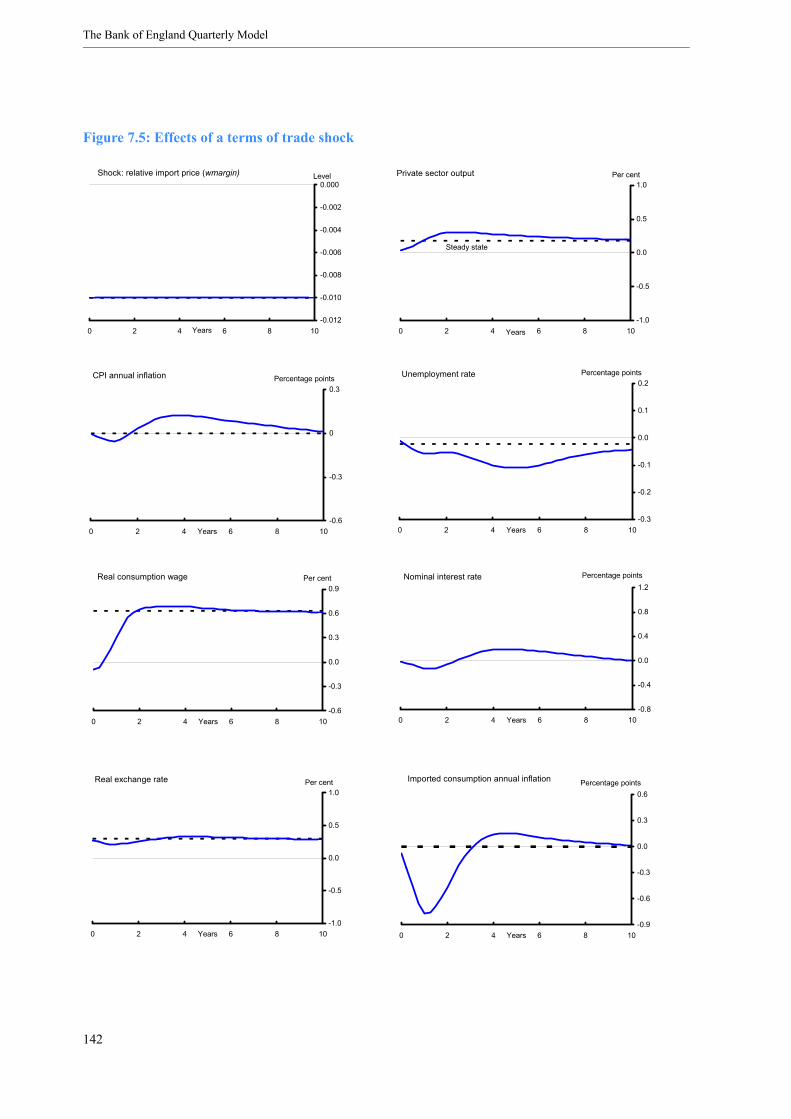
The Bank of England Quarterly Model
Figure 7.5: Effects of a terms of trade shock
Private sector output
-1.0
-0.5
0.0
0.5
1.0
0 2 4 6 8 10Years
Per cent
Steady state
CPI annual inflation
-0.6
-0.3
0
0.3
0 2 4 6 8 10Years
Percentage points Unemployment rate
-0.3
-0.2
-0.1
0.0
0.1
0.2
0 2 4 6 8 10Years
Percentage points
Real consumption wage
-0.6
-0.3
0.0
0.3
0.6
0.9
0 2 4 6 8 10Years
Per cent Nominal interest rate
-0.8
-0.4
0.0
0.4
0.8
1.2
0 2 4 6 8 10Years
Percentage points
Real exchange rate
-1.0
-0.5
0.0
0.5
1.0
0 2 4 6 8 10Years
Per cent Imported consumption annual inflation
-0.9
-0.6
-0.3
0.0
0.3
0.6
0 2 4 6 8 10Years
Percentage points
Shock: relative import price (wmargin)
-0.012
-0.010
-0.008
-0.006
-0.004
-0.002
0.000
0 2 4 6 8 10Years
Level
142
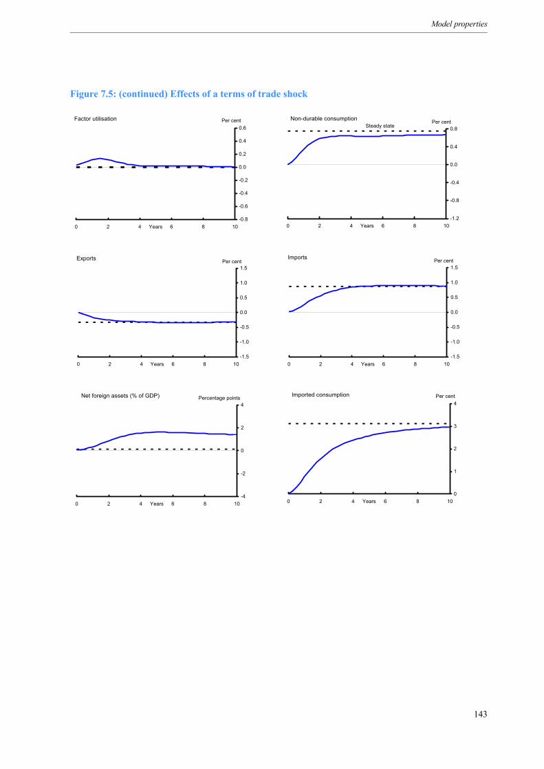
Model properties
Figure 7.5: (continued) Effects of a terms of trade shock
Non-durable consumption
-1.2
-0.8
-0.4
0.0
0.4
0.8
0 2 4 6 8 10Years
Per centSteady state
Exports
-1.5
-1.0
-0.5
0.0
0.5
1.0
1.5
0 2 4 6 8 10Years
Per centImports
-1.5
-1.0
-0.5
0.0
0.5
1.0
1.5
0 2 4 6 8 10Years
Per cent
Imported consumption
0
1
2
3
4
0 2 4 6 8 10Years
Per centNet foreign assets (% of GDP)
-4
-2
0
2
4
0 2 4 6 8 10Years
Percentage points
Factor utilisation
-0.8
-0.6
-0.4
-0.2
0.0
0.2
0.4
0.6
0 2 4 6 8 10Years
Per cent
143

The Bank of England Quarterly Model
7.2.5 A world demand shock
Figure 7.6 shows the effects of a permanent, unanticipated 1% increase in the level of world demand fordomestic goods. This simulation is particularly useful for highlighting the role of the real exchange rateand imported capital.
In a standard neoclassical model of a small open economy model, long-run supply is anchored by theworld real interest rate. An increase in export demand for UK goods and services would not be met by arise in output but would be completely offset by an increase in the real exchange rate. Neither is there ashort-run effect in many simple ‘textbook’ models, because the real exchange rate appreciation simplyoffsets the impact of higher world demand.
However, as described in Section 7.2.2, BEQM allows for the possibility that real exchange ratemovements can affect long-run supply. In the case of a world demand shock, the real exchange rateappreciates, which acts to reduce the cost of capital goods and raise the desired capital stock. Similarly,real consumption wages rise and labour supply increases. Both effects lead to an increase in output.
The long-run increase in real consumption wages and employment allows greater expenditure byhouseholds on non-durable consumption and investment in dwellings. Consumption, investment andgovernment spending move proportionally by slightly more than output. (32) Holdings of net foreignassets rise and the value of imports is lower in the long run (reflecting a relatively low price elasticity ofimport volumes), so a higher real exchange rate and a fall in export volumes is needed to balance thecurrent account. The shock effectively improves the economy’s relative earnings capability and netforeign asset position.
In the short run, the foreign currency price of domestic exports is slow to adjust to the increase in worlddemand. This fuels a short-run increase in export demand and, given slow adjustment of other demandcomponents, output immediately overshoots its long-run level. Factor utilisation rises as supplycapacity is relatively slow to adjust. Firms increase their demand for labour, reducing unemployment,and also increase prices. The exchange rate immediately appreciates close to its new long-run level,though the pass through to lower import prices is gradual. The net effect is for CPI inflation to rise alittle above target, to be brought down gradually over the longer term by a rise in interest rates.
(32)The model has a target for the ratio of nominal government spending to nominal private sector output. The movement ofrelative prices in this shock means that there are slightly different movements in the volumes of government spending and totaloutput.
144
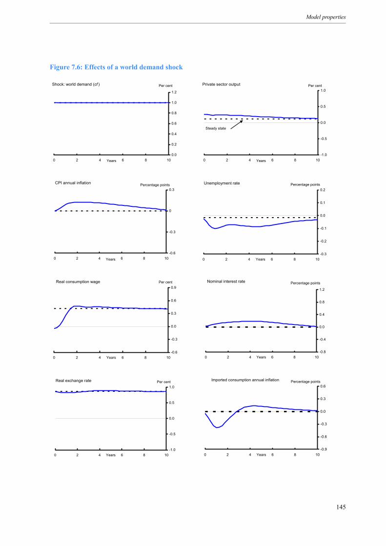
Model properties
Figure 7.6: Effects of a world demand shock
Private sector output
-1.0
-0.5
0.0
0.5
1.0
0 2 4 6 8 10Years
Per cent
Steady state
CPI annual inflation
-0.6
-0.3
0
0.3
0 2 4 6 8 10Years
Percentage points Unemployment rate
-0.3
-0.2
-0.1
0.0
0.1
0.2
0 2 4 6 8 10Years
Percentage points
Real consumption wage
-0.6
-0.3
0.0
0.3
0.6
0.9
0 2 4 6 8 10Years
Per cent Nominal interest rate
-0.8
-0.4
0.0
0.4
0.8
1.2
0 2 4 6 8 10Years
Percentage points
Real exchange rate
-1.0
-0.5
0.0
0.5
1.0
0 2 4 6 8 10Years
Per cent Imported consumption annual inflation
-0.9
-0.6
-0.3
0.0
0.3
0.6
0 2 4 6 8 10Years
Percentage points
Shock: world demand (cf )
0.0
0.2
0.4
0.6
0.8
1.0
1.2
0 2 4 6 8 10Years
Per cent
145
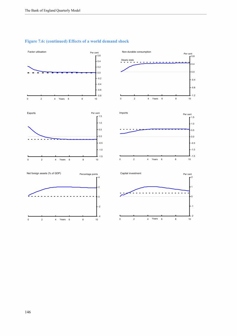
The Bank of England Quarterly Model
Figure 7.6: (continued) Effects of a world demand shock
Capital investment
-2
-1
0
1
2
0 2 4 6 8 10Years
Per cent
Non-durable consumption
-1.2
-0.8
-0.4
0.0
0.4
0.8
0 2 4 6 8 10Years
Per cent
Steady state
Exports
-1.5
-1.0
-0.5
0.0
0.5
1.0
1.5
0 2 4 6 8 10Years
Per cent Imports
-1.5
-1.0
-0.5
0.0
0.5
1.0
1.5
0 2 4 6 8 10Years
Per cent
Net foreign assets (% of GDP)
-4
-2
0
2
4
0 2 4 6 8 10Years
Percentage points
Factor utilisation
-0.8
-0.6
-0.4
-0.2
0.0
0.2
0.4
0.6
0 2 4 6 8 10Years
Per cent
146

Model properties
7.2.6 A labour market participation rate shock
Figure 7.7 shows the impact of a permanent decrease in labour market participation, such that theparticipation rate is lower at all real wage rates. (33) The simulation is interesting for the shock’s directeffects on supply and the equilibration of demand.
In a standard small open economy model, in which labour supply is exogenous and there is no importedcapital, a given drop in employment would be matched in the long run by a proportional fall in capitaland output. In BEQM, however, labour supply is endogenous and some final capital goods areimported. Therefore, the interaction between the real exchange rate and long-run supply discussed inSection 7.2.2 means that the decrease in labour supply, employment, capital stock and output is slightlyless than 1%. That is because the real consumption wage rises and the cost of capital goods falls.
Long-run aggregate labour income falls because the rise in the real consumption wage is less than thefall in employment. Consumption and housing investment fall, along with investment by firms andgovernment spending. (34) As total consumption and capital expenditures are reduced, imports fall too.But lower exports are needed to preserve external balance, so the real exchange rate appreciates.
As with the other shocks described in this chapter, these long-run effects on expenditure are reflected inchanges in asset positions. In addition to lower labour income, margins (and therefore profits anddividends) are squeezed as firms attempt to hold on to market share, so equity values fall. Net foreignassets are also reduced (even though there is a marginal rise in the ratio to output): the aggregateeconomy, in effect, borrows from overseas in an attempt to support aggregate consumption.
In the short run, the exchange rate appreciates immediately, to close to its new steady-state level.Participation and employment fall sharply over the first two years, along with consumption andinvestment. The supply of workers at every wage rate falls, so wages rise initially as firms try to preventemployment falling by as much as participation. The fall in labour participation is faster than that ofemployment, so the unemployment rate falls too in the short term. As employment and demand fall,firms initially reduce factor utilisation.
Import price inflation falls initially, because of the higher exchange rate. But domestic inflation rises asfirms have to bid wages up, and the real product wage rises substantially within the first two years. Thiseffect dominates the effect of cheaper imported goods and CPI inflation rises. Interest rates rise to bringinflation back to the target.
The results shown here accord qualitatively with the effects of a labour supply shock identified inPeersman and Straub (2004) for the euro area: hours and output fall, prices and real wages rise, andinterest rates rise temporarily. Despite the observed variation of unemployment with output over thebusiness cycle, there are few models that examine the joint behaviour of employment, unemploymentand labour market participation: Veracierto (2002) is one exception, using a matching framework, butthe results did not match observed dynamics in the US labour market.
(33)Technically, the shock is implemented as a reduction by 0.01 in the intercept term in the (log) labour supply schedule(equation (A.14) in Appendix A).(34) In this shock, the government spending target is expressed as a ratio to output, so spending falls in line with output.
147
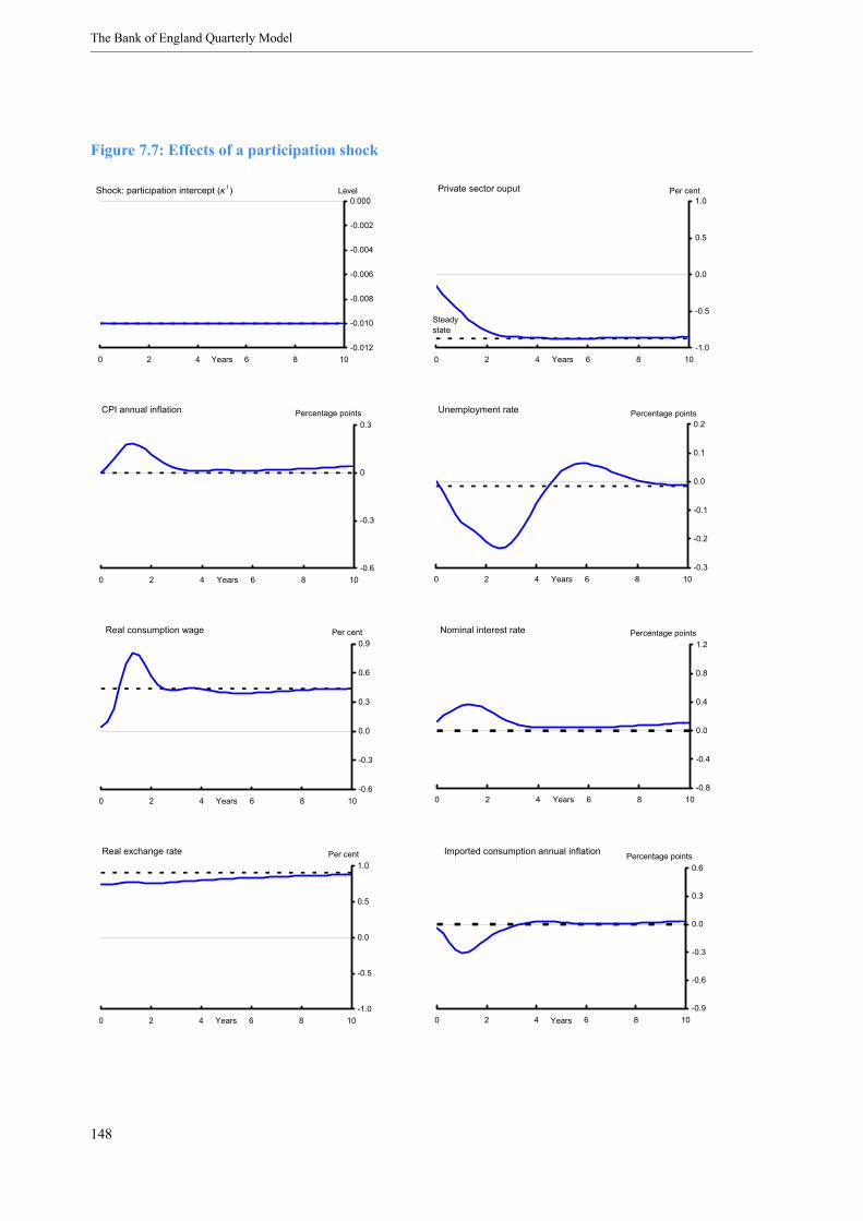
The Bank of England Quarterly Model
Figure 7.7: Effects of a participation shock
Private sector ouput
-1.0
-0.5
0.0
0.5
1.0
0 2 4 6 8 10Years
Per cent
Steady state
CPI annual inflation
-0.6
-0.3
0
0.3
0 2 4 6 8 10Years
Percentage points Unemployment rate
-0.3
-0.2
-0.1
0.0
0.1
0.2
0 2 4 6 8 10Years
Percentage points
Real consumption wage
-0.6
-0.3
0.0
0.3
0.6
0.9
0 2 4 6 8 10Years
Per cent Nominal interest rate
-0.8
-0.4
0.0
0.4
0.8
1.2
0 2 4 6 8 10Years
Percentage points
Real exchange rate
-1.0
-0.5
0.0
0.5
1.0
0 2 4 6 8 10Years
Per cent Imported consumption annual inflation
-0.9
-0.6
-0.3
0.0
0.3
0.6
0 2 4 6 8 10Years
Percentage points
Shock: participation intercept (κ l )
-0.012
-0.010
-0.008
-0.006
-0.004
-0.002
0.000
0 2 4 6 8 10Years
Level
148
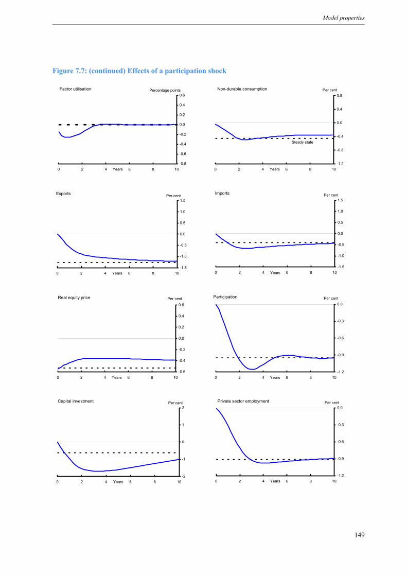
Model properties
Figure 7.7: (continued) Effects of a participation shock
Capital investment
-2
-1
0
1
2
0 2 4 6 8 10Years
Per cent
Non-durable consumption
-1.2
-0.8
-0.4
0.0
0.4
0.8
0 2 4 6 8 10Years
Per cent
Steady state
Exports
-1.5
-1.0
-0.5
0.0
0.5
1.0
1.5
0 2 4 6 8 10Years
Per cent Imports
-1.5
-1.0
-0.5
0.0
0.5
1.0
1.5
0 2 4 6 8 10Years
Per cent
Real equity price
-0.6
-0.4
-0.2
0.0
0.2
0.4
0.6
0 2 4 6 8 10Years
Per cent Participation
-1.2
-0.9
-0.6
-0.3
0.0
0 2 4 6 8 10Years
Per cent
Factor utilisation
-0.8
-0.6
-0.4
-0.2
0.0
0.2
0.4
0.6
0 2 4 6 8 10Years
Percentage points
Private sector employment
-1.2
-0.9
-0.6
-0.3
0.0
0 2 4 6 8 10Years
Per cent
149

The Bank of England Quarterly Model
7.3 Summary
This chapter illustrates the properties of the new model by describing a series of model simulations. Theresults must be used carefully, because they are stylised experiments that look at the marginal effects ofa single change, starting from an equilibrium position. And the effects of changes can be affectedsignificantly by different assumptions about how policy reacts and about agents’ expectations.
The reactions to a temporary shock to interest rates correspond to the broad conclusions of the empiricalliterature on monetary shocks: unanticipated policy tightening reduces output and then inflation. Thebehaviour is broadly similar to that of the previous MTMM model and close to other studies. As this isa temporary shock, there are no long-run effects on real variables or inflation. The effect of anunexpected change in interest rates on inflation is larger if agents believe that it is associated with achange in the targeted rate of inflation.
We then illustrate the interaction of long-run properties and short-run adjustment through shocks toproductivity, government spending, the terms of trade, world demand and labour market participation.As well as the conventional effects that would be expected from simple models, the results show howmovements in the real exchange rate can affect potential supply through changes in labour forceparticipation and the desired capital stock: other things being equal, a real exchange rate depreciationleads to a slight reduction in potential supply.
Short-term movements in the face of shocks illustrate the effects of immediate changes in asset pricescoupled with sluggish adjustment of employment, capital and prices. The simulations also show howthe policy reaction functions that we use outside of the forecast act to ensure fiscal solvency and to bringinflation back to target over the medium term.
150

Chapter 8 Final remarks
This book describes a new macroeconomic model that has been created for use in preparing theMonetary Policy Committee’s quarterly economic projections. Building the new model has been asubstantial investment for the Bank, and in this book we attempt to explain the model in some detail.The new macroeconomic model is by no means the only input into the forecasting and policy processes:the Committee continues to draw on a range of other information, including the Bank’s suite of models.Indeed, one of the intended benefits from the way in which the new model was built is that it should be abetter complement to the suite of models – it should be easier to compare assumptions and toincorporate off-model information and analysis.
The design of the new macroeconomic model reflects the demands of forecasting and policy analysis atthe Bank of England – a central bank where interest rate decisions are decided by the votes of acommittee to meet a specified inflation target. A key question in the design of the new model is whereto position the model in terms of a trade-off between theoretical rigour and accounting for observedcorrelations in the data. Two further issues are how to parameterise a large system such as this, and howto use the model for forecasting (such as the need to incorporate judgement and to ‘fix’ the paths ofsome endogenous variables). All of these posed challenges to the model design. There are certainlyalternative solutions to these problems, and it is likely that advances in computing technology will makesome of them (such as systems estimation) easier to deal with in the future.
One clear difference from the Bank’s previous macroeconomic model is the shift to a moremicro-founded theoretical structure, as embodied in the core model. We do not assume that the model isautomatically made believable by the use of micro-foundations; instead it meets the need for a clear andconsistent structure as the basis for differentiating between several possible explanations for theobserved behaviour of the economy.
The full forecasting model does not rely exclusively on the micro-founded core model. We can think ofthe forecast as a process that weights together three types of information: a structural story that comesfrom the core model; additional variables and robust correlations in the data that are not captured in thecore theory but that we might want to project forward; and direct adjustment made on the basis ofjudgement and ‘off-model’ information. This structure implies a progressive modelling agenda: if adhoc features are consistently important in producing a forecast, then an obvious aim is to incorporatethese features into the structural core model if possible.
This book documents the new macroeconomic model used by the MPC in the preparation of itseconomic projections. The new model does not represent a change in the Committee’s view of how theeconomy works or of the role of monetary policy. The model is not fixed, and will evolve over time:continuing maintenance and development will be required to deal with new issues and puzzles. TheBank has committed resources to this and also to the development of complementary models. At thesame time, a strategic objective of the Bank is to reap the benefits of the new model, using it not just forforecasting but also to aid our work on strategic issues relating to monetary policy.
151

References
Abel, A B (1990), ‘Asset Prices under Habit Formation and Catching up with the Joneses’, AmericanEconomic Review, Vol. 80(2), pages 38-42.
Adolfson, M, Laséen, S, Lindé, J and Villani, M (2004a), ‘Bayesian estimation on open econonyDSGE model with incomplete pass-through’, mimeo, Sveriges Riksbank.
Adolfson, M, Laséen, S, Lindé, J and Villani, M (2004b), ‘The role of sticky prices in an openeconomy DSGE model: A Bayesian investigation’, mimeo, Sveriges Riksbank.
Amano, R, McPhail, K, Pioro, H and Rennison, A (2002), ‘Evaluating the Quarterly ProjectionModel: A Preliminary Investigation’, Bank of Canada Working Paper no. 2002-20.
Anderson, G S (1999), ‘Accelerating Non Linear Perfect Foresight Model Solution by Exploiting theSteady State Linearization’, mimeo, Board of Governors of the Federal Reserve System.
Andrews, M J, Bell, D N F, Fisher, P G, Wallis, K F and Whitley, J D (1984),Models of the UKEconomy: A Review by the ESRC Macroeconomic Modelling Bureau, Oxford: Oxford University Press.
Andrews, M J, Bell, D N F, Fisher, P G, Wallis, K F and Whitley, J D (1985),Models of the UKEconomy: A Second Review by the ESRC Macroeconomic Modelling Bureau, Oxford: OxfordUniversity Press.
Andrews, M J, Fisher, P G, Longbottom, J A, Wallis, K F and Whitley, J D (1986),Models of theUK Economy: A Third Review by the ESRC Macroeconomic Modelling Bureau, Oxford: OxfordUniversity Press.
Aoki, K, Proudman, J and Vlieghe, G (2002), ‘House prices, consumption, and monetary policy: afinancial accelerator approach’, Bank of England Working Paper no. 169.
Attanasio, O P (1999), ‘Consumption Demand’, in Taylor, J B and Woodford, M (eds) Handbook ofMacroeconomics Vol. 1B, Amsterdam: North-Holland.
Banerjee, R and Batini, N (2003), ‘UK Consumers’ Habits’, Bank of England External MPC UnitDiscussion Paper no. 13.
Bank of England (1999a), Economic models at the Bank of England.
Bank of England (1999b), ‘The transmission mechanism of monetary policy’, Bank of EnglandQuarterly Bulletin, May, pages 161-70.
Bank of England (2000), Economic models at the Bank of England, September 2000 update.
Bank of England (2004), ‘The new Bank of England Quarterly Model’, Bank of England QuarterlyBulletin, Summer, pages 188-93.
Barro, R J and Sala-i-Martin, X (1995), Economic Growth, New York: McGraw-Hill.
153
The Bank of England Quarterly Model
Barry, F and Devereux, M B (2003), ‘Expansionary fiscal contraction: A theoretical exploration’,Journal of Macroeconomics, Vol. 25(1), pages 1-23.
Basu, S, Fernald, J G and Kimball, M S (1998), ‘Are technology improvements contractionary?’Board of Governors of the Federal Reserve International Finance Discussion Papers no. 625.
Basu, S and Kimball, M S (1997), ‘Cyclical Productivity with Unobserved Input Variation’, NationalBureau of Economic Research Working Paper no. 5915.
Batini, N, Harrison, R, and Millard, S P (2003), ‘Monetary policy rules for an open economy’,Journal of Economic Dynamics and Control, Vol. 27(11-12), pages 2059-94.
Batini, N and Nelson, E (2000), ‘Optimal horizons for inflation targeting’, Bank of England WorkingPaper no. 119.
Baxter, M and Farr, D D (2001), ‘Variable Factor Utilization and International Business Cycles’,National Bureau of Economic Research Working Paper no. 8392.
Bayoumi, T and Eichengreen, B J (1992), ‘Shocking Aspects of European Monetary Unification’,National Bureau of Economic Research Working Paper no. 3949.
Bean, C (1998), ‘The New UK Monetary Arrangements: A View from the Literature’, EconomicJournal, Vol. 108(451), pages 1795-1809.
Bean, C, Larsen, J D J, and Nikolov, K (2002), ‘Financial frictions and the monetary transmissionmechanism: theory, evidence and policy implications’, European Central Bank Working Paper no. 113.
Bergin, P R (2003), ‘Putting the “New Open Economy Macroeconomics” to a Test’, Journal ofInternational Economics, Vol. 60(1), pages 3-34.
Bernanke, B S, Gertler, M and Gilchrist, S (1996), ‘The Financial Accelerator and the Flight toQuality’, Review of Economics and Statistics, Vol. 78(1), pages 1-15.
Bernanke, B S, Gertler, M and Gilchrist, S (1999), ‘The Financial Accelerator in a QuantitativeBusiness Cycle Framework’, in Taylor, J B and Woodford, M (eds), Handbook of Macroeconomics Vol.1C, Amsterdam: North-Holland.
Black, R, Cassino, V, Drew, A, Hansen, E, Hunt, B, Rose, D and Scott, A (1997), ‘The Forecastingand Policy System: the core model’, Reserve Bank of New Zealand Research Paper no. 43.
Black, R, Laxton, D, Rose, D and Tetlow, R (1994), ‘The Steady-State Model: SSQPM, The Bank ofCanada’s New Quarterly Projection Model, Part 1’, Bank of Canada Technical Report no. 72.
Blanchard, O J (1985), ‘Debt, Deficits and Finite Horizons’, Journal of Political Economy, Vol. 93(2),pages 223-47.
Blanchard, O J and Kahn, C M (1980), ‘The Solution of Linear Difference Models under RationalExpectations’, Econometrica, Vol. 48(5), pages 1305-11.
154

References
Blanchard, O J and Kiyotaki, N (1987), ‘Monopolistic Competition and the Effects of AggregateDemand’, American Economic Review, Vol. 77(4), pages 647-66.
Blanchard, O J and Perotti, R (2002), ‘An Empirical Characterization of the Dynamic Effects ofChanges in Government Spending and Taxes on Output’, Quarterly Journal of Economics, Vol. 117(4),pages 1329-68.
Boucekkine, R (1995), ‘An alternative method for solving nonlinear forward-looking models’, Journalof Economic Dynamics and Control, Vol. 19(4), pages 711-34.
Brayton, F and Tinsley, P (eds) (1996), ‘A guide to FRB/US: A Macroeconomic Model of the UnitedStates’, Federal Reserve Board Finance and Economics Discussion Series no. 1996-42.
Broda, C (2001), ‘Coping with Terms-of-Trade Shocks: Pegs versus Floats’, American EconomicReview, Vol. 91(2), pages 376-80.
Browning, M, Hansen, L P and Heckman, J J (1999), ‘Micro Data and General Equilibrium Models’,in Taylor, J B and Woodford, M (eds) Handbook of Macroeconomics Vol. 1A, Amsterdam:North-Holland.
Budd, A, Dicks, G, Holly, S, Keating, G and Robinson, B (1984), ‘The London Business SchoolEconometric Model of the UK’, Economic Modelling, Vol. 1(4), pages 355-420.
Buiter, W H (1988), ‘Death, Birth, Productivity Growth and Debt Neutrality’, The Economic Journal,Vol. 98(391), pages 279-93.
Burnside, C and Eichenbaum, M (1996), ‘Factor-Hoarding and the Propagation of Business-CycleShocks’, American Economic Review, Vol. 86(5), pages 1154-74.
Burnside, C, Eichenbaum, M and Fisher, J D M (2002), ‘Assessing the effects of fiscal shocks’,mimeo.
Calvo, G A (1983), ‘Staggered prices in a utility-maximising framework’, Journal of MonetaryEconomics, Vol. 12(3), pages 383-98.
Canova, F (1994), ‘Statistical inference in calibrated models’, Journal of Applied Econometrics, Vol. 9,pages S123-44.
Canova, F (1995), ‘Sensitivity Analysis and Model Evaluation in Simulated Dynamic GeneralEquilibrium Economies’, International Economic Review, Vol. 36(2), pages 477-501.
Canova, F, Finn, M and Pagan, A R (1994), ‘Evaluating a Real Business Cycle Model’, in Hargreaves,C P (ed), Non-Stationary Time Series Analysis and Cointegration, Oxford: Oxford University Press.
Cavallo, M (2002), ‘Government Employment and the Dynamic Effects of Fiscal Policy Shocks’,mimeo, New York University.
Chong, Y Y and Hendry, D F (1986), ‘Econometric Evaluation of Linear Macroeconomic Models’,Review of Economic Studies, Vol. 53(4), pages 671-90.
155
The Bank of England Quarterly Model
Christiano, L J, Eichenbaum, M and Evans, C L (1997), ‘Sticky price and limited participationmodels: A comparision’, European Economic Review, Vol. 41(6), pages 1201-49.
Christiano, L J, Eichenbaum, M and Evans, C L (1999), ‘Monetary policy shocks: what have welearned and to what end?’, in Taylor, J B and Woodford, M (eds) Handbook of Macroeconomics Vol. 1A,Amsterdam: North-Holland.
Christiano, L J, Eichenbaum, M and Evans, C L (2001), ‘Nominal rigidities and the dynamic effectsof a shock to monetary policy’, National Bureau of Economic Research Working Paper no. 8403.
Christiano, L J, Eichenbaum, M and Vigfusson, R (2003), ‘What happens after a technology shock?’,National Bureau of Economic Research Working Paper no. 9819.
Church, K B, Mitchell, P R, Sault, J E and Wallis, K F (1997), ‘Comparative properties of models ofthe UK economy’, National Institute Economic Review, No. 161, July, pages 91-100.
Church, K B, Mitchell, P R, Smith, P N and Wallis, K F (1993), ‘Comparative properties of modelsof the UK economy’, National Institute Economic Review, No. 145, August, pages 87-107.
Church, K B, Mitchell, P R, Smith, P N and Wallis, K F (1995), ‘Comparative properties of modelsof the UK economy’, National Institute Economic Review, No. 153, August, pages 59-72.
Church, K B, Mitchell, P R, Turner, D S, Wallis, K F and Whitley, J D (1991), ‘Comparativeproperties of models of the UK economy’, National Institute Economic Review, No. 137, August, pages59-74.
Church, K B, Sault, J E, Sgherri, S and Wallis, K F (2000), ‘Comparative properties of models of theUK economy’, National Institute Economic Review, No. 171, January, pages 106-22.
Cochrane, J H (1993), ‘Solving real business cycle models by solving systems of first orderconditions’, mimeo, Graduate School of Business, University of Chicago.
Coletti, D, Hunt, B, Rose, D and Tetlow, R (1996), ‘The Dynamic Model: QPM, The Bank ofCanada’s New Quarterly Projection Model, Part 3’, Bank of Canada Technical Report no. 75.
Cooper, J P and Nelson, C R (1975), ‘The Ex Ante Prediction Performance Of the St. Louis andFRB-MIT-PENN Econometric Models and Some Results on Composite Predictors’, Journal of Money,Credit and Banking, Vol. 7(1), pages 1-32.
Cromb, R and Fernandez-Corugedo, E (2004), ‘Long-term interest rates, wealth and consumption’,Bank of England Working Paper no. 243.
Cushman, D O and Zha, T (1995), ‘Identifying monetary policy in a small open economy underflexible exchange rates’, Federal Reserve Bank of Atlanta Working Paper no. 95-7.
Dale, S and Haldane, A G (1995), ‘Interest rates and the channels of monetary transmission: Somesectoral estimates’, European Economic Review, Vol. 39(9), pages 1611-26.
Darby, J, Ireland, J, Leith, C and Wren-Lewis, S (1999), ‘COMPACT: a rational expectations,intertemporal model of the United Kingdom economy’, Economic Modelling, Vol. 16(1), pages 1-52.
156

References
Davidson, R, and MacKinnon, J G (1993), Estimation and Inference in Econometrics. New York:Oxford University Press.
De Gregorio, J and Wolf, H C (1994), ‘Terms of Trade, Productivity, and the Real Exchange Rate’,National Bureau of Economic Research Working Paper no. 4807.
Del Negro, M and Schorfheide, F (2004), ‘Priors from General Equilibrium Models for VARs’,International Economic Review, Vol. 45(2), pages 643-73.
Diebold, F X and Lopez, J A (1996), ‘Forecast Evaluation and Combination’, in Maddala, G S andRao, C R (eds), Handbook of Statistics, Amsterdam: North-Holland.
Diebold, F X and Mariano, R S (1995), ‘Comparing predictive accuracy’, Journal of Business andEconomic Statistics, Vol. 13(3), pages 253-63.
Dinenis, E, Holly, S, Levine, P and Smith, P (1989), ‘The London Business School econometricmodel: Some recent developments’, Economic Modelling, Vol. 6(3), pages 243-351.
Dixit, A K and Stiglitz, J E (1977), ‘Monopolistic Competition and Optimum Product Diversity’,American Economic Review, Vol. 67(3), pages 297-308.
Doornik, J A and Hendry, D F (1994), ‘Modelling Linear Dynamic Econometric Systems’, ScottishJournal of Political Economy, Vol. 41(1), pages 1-33.
Edge, R M, Laubach, T andWilliams, J C (2003), ‘The Responses of Wages and Prices to TechnologyShocks’, Federal Reserve Board of Governors Finance and Economics Discussion Series no. 2003-65.
Eichenbaum, M (1995), ‘Some Comments on the Role of Econometrics in Economic Theory’, TheEconomic Journal, Vol. 105(433), 1609-21.
Erceg, C J, Guerrieri, L and Gust, C J (2004), ‘Expansionary Fiscal Shocks and the Current Account’mimeo, Board of Governors of the Federal Reserve System.
Erceg, C J, Henderson, D W and Levin, A T (2000), ‘Optimal monetary policy with staggered wageand price contracts’, Journal of Monetary Economics, Vol. 46(2), pages 281-313.
Erceg, C J and Levin, A T (2003), ‘Imperfect credibility and inflation persistence’, Journal ofMonetary Economics, Vol. 50 (4), pages 915-44.
Fair, R C (1993), ‘Testing the Rational Expectations Hypothesis in Macroeconometric Models’, OxfordEconomic Papers, Vol. 45(2), pages 169-90.
Fair, R C (1994), Testing Macroeconometric Models, Cambridge, MA: Harvard University Press.
Favero, C A and Hendry, D F (1992), ‘Testing the Lucas Critique: A Review’, Econometric Reviews,Vol. 11(3), pages 265-306.
Fernández-Villaverde, J and Rubio-Ramírez, J F (2004), ‘Comparing dynamic equilibrium models todata: a Bayesian approach’, Journal of Econometrics, Vol 123(1), pages 153-87.
157
The Bank of England Quarterly Model
Fisher, J D M and Hornstein, A (2000), ‘(S, s) Inventory Policies in General Equilibrium’, Review ofEconomic Studies, Vol. 67(1), pages 117-45.
Fisher, P G, Holly, S and Hughes-Hallett, A J (1986), ‘Efficient solution techniques for dynamicnon-linear rational expectations models’, Journal of Economic Dynamics and Control, Vol. 10(1-2),pages 139-45.
Fisher, P G, Longbottom, J A, Turner D S, Wallis, K F and Whitley, J D (1987), Models of the UKEconomy: A Fourth Review by the ESRC Macroeconomic Modelling Bureau, Oxford: Oxford UniversityPress.
Fisher, P G, Tanna, S K, Turner, D S, Wallis, K F and Whitley, J D (1989), ‘Comparative propertiesof models of the UK economy’, National Institute Economic Review, No. 129, August, pages 69-87.
Fisher, P G, Turner, D S, Wallis, K F and Whitley, J D (1990), ‘Comparative properties of models ofthe UK economy’, National Institute Economic Review, No. 133, August, pages 91-104.
Frenkel, J A and Razin, A (1996), Fiscal Policies and Growth in the World Economy (3rd edition),Cambridge, MA: MIT Press.
Fuhrer, J C (2000), ‘Habit Formation in Consumption and Its Implications for Monetary PolicyModels’, American Economic Review, Vol. 90(3), pages 367-90.
Fujiwara, I, Hara, N, Hirose, Y and Teranishi, Y (2004), ‘The Japanese Economic Model: JEM’.Bank of Japan Working Paper no. 04-E-3.
Galí, J (1996), ‘Unemployment in dynamic general equilibrium economies’, European EconomicReview, Vol. 40(3-5), pages 839-45.
Galí, J (1999), ‘Technology, Employment, and the Business Cycle: Do Technology Shocks ExplainAggregate Fluctuations?’, American Economic Review, Vol. 89(1), pages 249-71.
Galí, J, Gertler, M and López-Salido, J D (2001), ‘European inflation dynamics’, European EconomicReview, Vol. 45(7), pages 1237-70.
Hall, S (2001), ‘Financial effects on corporate investment in UK business cycles’, Bank of EnglandQuarterly Bulletin, Winter, pages 449-59.
Hall, S G (1986), ‘Time inconsistency and optimal policy formulation in the presence of rationalexpectations’, Journal of Economic Dynamics and Control, Vol. 10(1-2), pages 323-26.
Hall, S G and Henry, S G B (1985), ‘Rational expectations in an econometric model: NIESR Model 8’,National Institute Economic Review, No. 114, November, pages 58-68.
Hall, S G and Henry, S G B (1986), ‘A dynamic econometric model of the UK with rationalexpectations’, Journal of Economic Dynamics and Control, Vol. 10(1-2), pages 219-23.
Hall, S G and Henry, S G B (1987),Macroeconomic Modelling, Amsterdam: North-Holland.
158
References
Hamilton, J D (1994), Time Series Analysis, Princeton: Princeton University Press.
Hansen, G D (1985), ‘Indivisible labor and the business cycle’, Journal of Monetary Economics, Vol.16(3), pages 309-27.
Harvey, D I, Leybourne, S J and Newbold, P (1997), ‘Testing the equality of prediction mean squareerrors’, International Journal of Forecasting, Vol. 13(2), pages 281-91.
Hendry, D F and Mizon, G E (1993), ‘Evaluating Dynamic Econometric Models by Encompassing theVAR’, in Phillips P C B (ed),Models, Methods and Applications of Econometrics, Oxford: BasilBlackwell.
Holly, S (1986), ‘Games, expectations, and optimal policy for open economies’, Journal of EconomicDynamics and Control, Vol. 10(1-2), pages 45-49.
Holly, S and Zarrop, M B (1983), ‘On optimality and time consistency when expectations are rational’,European Economic Review, Vol. 20(1), pages 23-40.
Hunt, B, Rose, D and Scott, A (2000), ‘The core model of the Reserve Bank of New Zealand’sForecasting and Policy System’, Economic Modelling, Vol. 17(2), pages 247-74.
Ingram, B F and Whiteman, C H (1994), ‘Supplanting the ‘Minnesota’ prior: Forecastingmacroeconomic time series using real business cycle model priors’, Journal of Monetary Economics,Vol. 34(3), pages 497-510.
Ireland, P N (2004), ‘A method for taking models to the data’, Journal of Economic Dynamics andControl, Vol. 28(6), pages 1205-26.
Judd, K L (2002), ‘The parametric path method: an alternative to Fair-Taylor and L-B-J for solvingperfect foresight models’, Journal of Economic Dynamics and Control, Vol. 26(9-10), pages 1557-83.
Juillard, M (1996), ‘DYNARE: A program for the resolution and simulation of dynamic models withforward variables through the use of a relaxation algorithm’, CEPREMAP Working Paper no. 9602.
Juillard, M, Karam, P, Laxton, D and Pesenti, P (2004), ‘Welfare-Based Monetary Policy Rules in anEstimated DSGE Model of the US Economy’, mimeo, Federal Reserve Bank of New York.
Kahn, A and Thomas, J K (2003), ‘Inventories and the Business Cycle: An Equilibrium Analysis of(S,s) Policies’, National Bureau of Economic Research Working Paper no. 10078.
Kahn, J A (1987), ‘Inventories and the Volatility of Production’, American Economic Review, Vol.77(4), pages 667-79.
Kapetanios, G, Pagan, A R and Scott, A (2004), ‘Making a match’, mimeo.
Kim, K and Pagan, A R (1995), ‘The Econometric Analysis of Calibrated Macroeconomic Models’, inPesaran, M H and Wickens M R (eds), Handbook of Applied Econometrics, Oxford: Blackwell.
King, R G, Plosser, C I and Rebelo, S T (1988), ‘Production, growth and business cycles: I. the BasicNeoclassical Model’, Journal of Monetary Economics, Vol. 21(2-3), pages 195-232.
159
The Bank of England Quarterly Model
Klein, L (1950), Economic Fluctuations in the United States, 1921-1941, New York: John Wiley andSons.
Kozicki, S and Tinsley, P A (1999), ‘Vector rational error correction’, Journal of Economic Dynamicsand Control, Vol. 23 (9-10), pages 1299-1327.
Kwiatkowski, D, Phillips, P C B, Schmidt, P and Shin, Y (1992), ‘Testing the null hypothesis ofstationarity against the alternative of a unit root: How sure are we that economic time series have a unitroot?’, Journal of Econometrics, Vol. 54, pages 159–78.
Laffargue, J-P (1990), ‘Résolution d’un modèle macroéconomique avec anticipations rationnelles’,Annales d’Économie et de Statistique, Vol. 17, pages 97-119.
Lagarias, J C, Reeds, J A, Wright, M H and Wright, P E (1998), ‘Convergence Properties of theNelder-Mead Simplex Method in Low Dimensions’, SIAM Journal on Optimization, Vol. 9(1), pages112-47.
Laxton, D M, Isard, P, Faruqee, H, Prasad, E S and Turtleboom, B (1998), ‘MULTIMOD Mark III:The Core Dynamic and Steady-State Models’, International Monetary Fund Occassional Paper no. 164.
Layard, R, Nickell, S J and Jackman, R (1991), Unemployment - Macroeconomic Performance andthe Labour Market, Oxford: Oxford University Press.
Leeper, E M (1997), ‘Narrative and VAR approaches to monetary policy: Common identificationproblems’, Journal of Monetary Economics, Vol. 40(3), pages 641-57.
Leeper, E M, Sims, C A and Zha, T (1996), ‘What Does Monetary Policy Do?’, Brookings Papers onEconomic Activity, Vol. 1996(2), pages 1-63.
Leeper, E M and Zha, T (2003), ‘Modest policy interventions’, Journal of Monetary Economics, Vol.50(8), pages 1673-1700.
Lucas, R E (1987),Models of Business Cycles, Oxford: Basil Blackwell.
Lynch, B and Whitaker, S (2004), ‘The new sterling ERI’, Bank of England Quarterly Bulletin, Winter,pages 429-41.
Mankiw, N G (1985), ‘Small Menu Costs and Large Business Cycles: A Macroeconomic Model ofMonopoly’, Quarterly Journal of Economics, Vol. 100(2), pages 529-37.
Manning, A (1993), ‘Wage Bargaining and the Phillips Curve: the Identification and Specification ofAggregate Wage Equations’, The Economic Journal, Vol. 103(416), pages 98-118.
McKibbin, W J, Pagan, A R and Robertson, J C (1998), ‘Some experiments in constructing a hybridmodel for macroeconomic analysis’, Carnegie-Rochester Conference Series on Public Policy, Vol. 49,pages 113-42.
Minford, A P L (1980), ‘A rational expectations model of the United Kingdom under fixed and floatingexchange rates’, Carnegie-Rochester Conference Series on Public Policy, Vol. 12, pages 293-355.
160

References
Monticelli, C and Tristani, O (1999), ‘What Does the Single Monetary Policy Do? A SVARBenchmark Model for the European Central Bank’, European Central Bank Working Paper no. 2.
Moran, K and Dolar, V (2002), ‘Estimated DGE Models and Forecasting Accuracy: A PreliminaryInvestigation with Canadian Data’, Bank of Canada Working Paper no. 2002-18.
Mortensen, D T and Pissarides, C A (1994), ‘Job Creation and Job Destruction in the Theory ofUnemployment’, Review of Economic Studies, Vol. 61(3), pages 397-415.
Nelson, C R (1972), ‘The Prediction Performance of the FRB-MIT-PENN Model of the U.S. Economy’,American Economic Review, Vol. 62(5), pages 902-17.
Nelson, E and Nikolov, K (2002), ‘Monetary policy and stagflation in the UK’, Bank of EnglandWorking Paper no. 155.
Nickell, S J (1985), ‘Error correction, partial adjustment and all that: an expository note’, OxfordBulletin of Economics and Statistics, Vol. 47(2), pages 119-29.
Obstfeld, M and Rogoff, K S (1996), Foundations of International Macroeconomics, Cambridge, MA:MIT Press.
Orphanides, A and Solow, R M (1990), ‘Money, Inflation and Growth’, in Friedman, B M and Hahn, FH (eds), Handbook of Monetary Economics, Amsterdam: North-Holland.
Oxley, L and McAleer, M (1993), ‘Econometric Issues in Macroeconomic Models with GeneratedRegressors’, Journal of Economic Surveys, Vol. 7(1), pages 1-40.
Pagan, A R (1984), ‘Econometric issues in the analysis of regressions with generated regressors’,International Economic Review, Vol. 25(1), pages 221-47.
Pagan, A R (2003), ‘Report on modelling and forecasting at the Bank of England’, Bank of EnglandQuarterly Bulletin, Spring, pages 60-88.
Peersman, G and Straub, R (2004), ‘Technology shocks and robust sign restrictions in a Euro areaSVAR’, European Central Bank Working Paper no. 373.
Perotti, R (2002), ‘Estimating the effects of fiscal policy in OECD countries’, mimeo.
Pesenti, P (2002), ‘The IMF Global Economy Model (GEM): Theoretical Framework’, mimeo,International Monetary Fund.
Ramey, V A and Shapiro, M D (1998), ‘Costly capital reallocation and the effects of governmentspending’, Carnegie Rochester Series on Public Policy, Vol. 48, pages 145-94.
Roeger, W and in’t Veld, J (1997), ‘QUEST II: A Multi Country Business Cycle and Growth Model’,European Commission Economic Papers no. 123.
Romer, D (1995), Advanced Macroeconomics, New York: McGraw-Hill.
161
The Bank of England Quarterly Model
Rotemberg, J J (1982), ‘Sticky Prices in the United States’, Journal of Political Economy, Vol. 90(6),pages 1187-1211.
Rotemberg, J J and Woodford, M (1999), ‘The cyclical behaviour of prices and costs’, in Taylor, J Band Woodford, M (eds) Handbook of Macroeconomics Vol. 1B, Amsterdam: North-Holland.
Roubini, N (1988), ‘Current Account and Budget Deficits in an Intertemporal Model of Consumptionand Taxation Smoothing. A Solution to the "Feldstein-Horioka Puzzle"?’, National Bureau of EconomicResearch Working Paper no. 2773.
Roubini, N and Kim, S (2003), ‘Twin Deficit or Twin Divergence? Fiscal Policy, Current Account, andReal Exchange Rate in the US’, mimeo, New York University.
Sargent, T J (1989), ‘Two Models of Measurements and the Investment Accelerator’, Journal ofPolitical Economy, Vol. 97(2), pages 251-87.
Sargent, T J and Ljungqvist, L (2000), Recursive Macroeconomic Theory, Cambridge, MA: MITPress.
Schmitt-Grohé, S and Uribe, M (2003), ‘Closing small open economy models’, Journal ofInternational Economics, Vol. 61(1), pages 163-85.
Schorfheide, F (1999), ‘A Unified Econometric Framework for the Evaluation of DSGE Models’, PennInstitute for Economic Research Working Paper no. 99-007.
Sims, C A (1972), ‘The Role of Approximate Prior Restrictions in Distributed Lag Estimation’, Journalof the American Statistical Association, Vol. 67, pages 169-75.
Sims, C A (2002), ‘The Role of Models and Probabilities in the Monetary Policy Process’, BrookingsPapers on Economic Activity, Vol. 2002(2), pages 1-40.
Smets, F R and Wouters, R (2003a), ‘An Estimated Dynamic Stochastic General Equilibrium Model ofthe Euro Area’, Journal of the European Economic Association, Vol. 1(5), pages 1123-75.
Smets, F R and Wouters, R (2003b), ‘Forecasting with a Bayesian DSGE Model: an Application to theEuro Area’, mimeo, European Central Bank and National Bank of Belgium.
Smets, F and Wouters, R (2004), ‘Shocks and frictions in US business cycles: A Bayesian DSGEapproach’, mimeo.
Stiglitz, J E (1979), ‘Equilibrium in Product Markets with Imperfect Information’, American EconomicReview, Vol. 69(2), pages 339-45.
Taylor, J B (1980), ‘Aggregate Dynamics and Staggered Contracts’, Journal of Political Economy, Vol.88(1), pages 1-23.
Theil, H (1961), Economic Forecasts and Policy, Amsterdam: North-Holland.
Turnovsky, S J (2000),Methods of Macroeconomic Dynamics, Cambridge, MA: MIT Press.
162

References
Veracierto, M (2002), ‘On the Cyclical Behavior of Employment, Unemployment and Labor ForceParticipation’, Federal Reserve Bank of Chicago Working Paper no. 2002-12.
Wallis, K F (1980), ‘Econometric Implications of the Rational Expectations Hypothesis’,Econometrica, Vol. 48(1), pages 49-73.
Wallis, K F and Whitley, J D (1991), ‘Macro models and macro policy’, Oxford Review of EconomicPolicy, Vol. 7(3), pages 118-27.
Walsh, C E (2003),Monetary Theory and Policy (2nd edition), Cambridge, MA: MIT Press.
Watson, MW (1993), ‘Measures of fit for calibrated models’, Journal of Political Economy, Vol.101(6), pages 1011-40.
Woodford, M (2003), Interest and Prices: Foundations of a Theory of Monetary Policy, Princeton:Princeton University Press.
Wolman, A L (1999), ‘Sticky Prices, Marginal Cost, and the Behavior of Inflation’, Federal ReserveBank of Richmond Economic Quarterly, Vol. 85(4), pages 29-48.
Wren-Lewis, S (1989), ‘Recent developments in the Institute’s Domestic Macromodel’, NationalInstitute Economic Review, No. 130, pages 47-51.
Yaari, M E (1965), ‘Uncertain Lifetime, Life Insurance, and the Theory of the Consumer’, Review ofEconomic Studies, Vol. 32(2), pages 137-50.
163

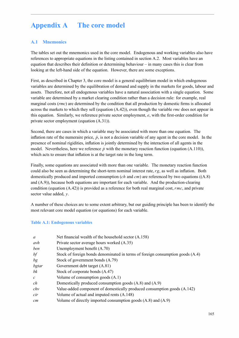
Appendix A The core model
A.1 Mnemonics
The tables set out the mnemonics used in the core model. Endogenous and working variables also havereferences to appropriate equations in the listing contained in section A.2. Most variables have anequation that describes their definition or determining behaviour – in many cases this is clear fromlooking at the left-hand side of the equation. However, there are some exceptions.
First, as described in Chapter 3, the core model is a general equilibrium model in which endogenousvariables are determined by the equilibration of demand and supply in the markets for goods, labour andassets. Therefore, not all endogenous variables have a natural association with a single equation. Somevariable are determined by a market clearing condition rather than a decision rule: for example, realmarginal costs (rmc) are determined by the condition that all production by domestic firms is allocatedacross the markets to which they sell (equation (A.42)), even though the variable rmc does not appear inthis equation. Similarly, we reference private sector employment, e, with the first-order condition forprivate sector employment (equation (A.31)).
Second, there are cases in which a variable may be associated with more than one equation. Theinflation rate of the numeraire price, p, is not a decision variable of any agent in the core model. In thepresence of nominal rigidities, inflation is jointly determined by the interaction of all agents in themodel. Nevertheless, here we reference p with the monetary reaction function (equation (A.110)),which acts to ensure that inflation is at the target rate in the long term.
Finally, some equations are associated with more than one variable. The monetary reaction functioncould also be seen as determining the short-term nominal interest rate, rg, as well as inflation. Bothdomestically produced and imported consumption (ch and cm) are referenced by two equations ((A.8)and (A.9)), because both equations are important for each variable. And the production-clearingcondition (equation (A.42)) is provided as a reference for both real marginal cost, rmc, and privatesector value added, y.
A number of these choices are to some extent arbitrary, but our guiding principle has been to identify themost relevant core model equation (or equations) for each variable.
Table A.1: Endogenous variables
a Net financial wealth of the household sector (A.158)avh Private sector average hours worked (A.35)ben Unemployment benefit (A.70)bf Stock of foreign bonds denominated in terms of foreign consumption goods (A.4)bg Stock of government bonds (A.79)bgtar Government debt target (A.81)bk Stock of corporate bonds (A.47)c Volume of consumption goods (A.1)ch Domestically produced consumption goods (A.8) and (A.9)chv Value-added component of domestically produced consumption goods (A.142)cir Volume of actual and imputed rents (A.148)cm Volume of directly imported consumption goods (A.8) and (A.9)
165
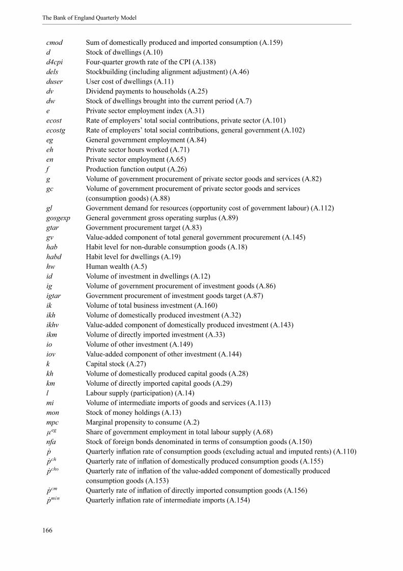
The Bank of England Quarterly Model
cmod Sum of domestically produced and imported consumption (A.159)d Stock of dwellings (A.10)d4cpi Four-quarter growth rate of the CPI (A.138)dels Stockbuilding (including alignment adjustment) (A.46)duser User cost of dwellings (A.11)dv Dividend payments to households (A.25)dw Stock of dwellings brought into the current period (A.7)e Private sector employment index (A.31)ecost Rate of employers’ total social contributions, private sector (A.101)ecostg Rate of employers’ total social contributions, general government (A.102)eg General government employment (A.84)eh Private sector hours worked (A.71)en Private sector employment (A.65)f Production function output (A.26)g Volume of government procurement of private sector goods and services (A.82)gc Volume of government procurement of private sector goods and services
(consumption goods) (A.88)gl Government demand for resources (opportunity cost of government labour) (A.112)gosgexp General government gross operating surplus (A.89)gtar Government procurement target (A.83)gv Value-added component of total general government procurement (A.145)hab Habit level for non-durable consumption goods (A.18)habd Habit level for dwellings (A.19)hw Human wealth (A.5)id Volume of investment in dwellings (A.12)ig Volume of government procurement of investment goods (A.86)igtar Government procurement of investment goods target (A.87)ik Volume of total business investment (A.160)ikh Volume of domestically produced investment (A.32)ikhv Value-added component of domestically produced investment (A.143)ikm Volume of directly imported investment (A.33)io Volume of other investment (A.149)iov Value-added component of other investment (A.144)k Capital stock (A.27)kh Volume of domestically produced capital goods (A.28)km Volume of directly imported capital goods (A.29)l Labour supply (participation) (A.14)mi Volume of intermediate imports of goods and services (A.113)mon Stock of money holdings (A.13)mpc Marginal propensity to consume (A.2)µeg Share of government employment in total labour supply (A.68)nfa Stock of foreign bonds denominated in terms of consumption goods (A.150)p Quarterly inflation rate of consumption goods (excluding actual and imputed rents) (A.110)pch Quarterly rate of inflation of domestically produced consumption goods (A.155)pchv Quarterly rate of inflation of the value-added component of domestically produced
consumption goods (A.153)pcm Quarterly rate of inflation of directly imported consumption goods (A.156)pmin Quarterly inflation rate of intermediate imports (A.154)
166
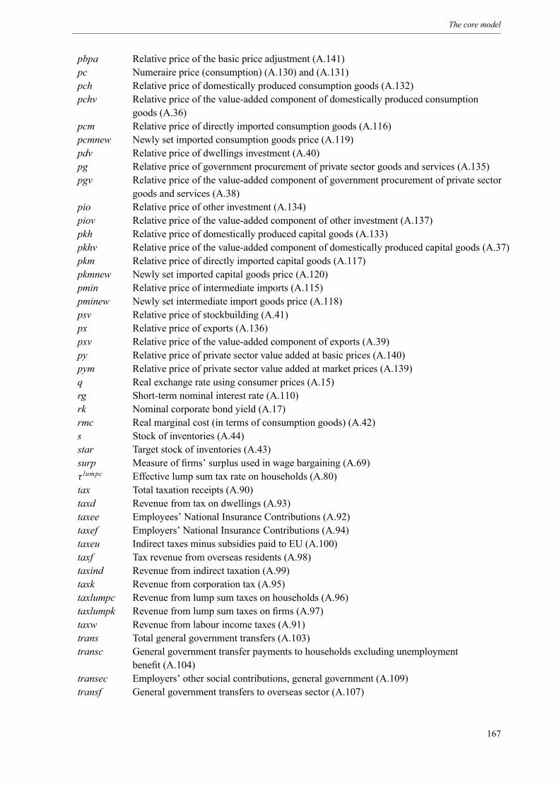
The core model
pbpa Relative price of the basic price adjustment (A.141)pc Numeraire price (consumption) (A.130) and (A.131)pch Relative price of domestically produced consumption goods (A.132)pchv Relative price of the value-added component of domestically produced consumption
goods (A.36)pcm Relative price of directly imported consumption goods (A.116)pcmnew Newly set imported consumption goods price (A.119)pdv Relative price of dwellings investment (A.40)pg Relative price of government procurement of private sector goods and services (A.135)pgv Relative price of the value-added component of government procurement of private sector
goods and services (A.38)pio Relative price of other investment (A.134)piov Relative price of the value-added component of other investment (A.137)pkh Relative price of domestically produced capital goods (A.133)pkhv Relative price of the value-added component of domestically produced capital goods (A.37)pkm Relative price of directly imported capital goods (A.117)pkmnew Newly set imported capital goods price (A.120)pmin Relative price of intermediate imports (A.115)pminew Newly set intermediate import goods price (A.118)psv Relative price of stockbuilding (A.41)px Relative price of exports (A.136)pxv Relative price of the value-added component of exports (A.39)py Relative price of private sector value added at basic prices (A.140)pym Relative price of private sector value added at market prices (A.139)q Real exchange rate using consumer prices (A.15)rg Short-term nominal interest rate (A.110)rk Nominal corporate bond yield (A.17)rmc Real marginal cost (in terms of consumption goods) (A.42)s Stock of inventories (A.44)star Target stock of inventories (A.43)surp Measure of firms’ surplus used in wage bargaining (A.69)τ lumpc Effective lump sum tax rate on households (A.80)tax Total taxation receipts (A.90)taxd Revenue from tax on dwellings (A.93)taxee Employees’ National Insurance Contributions (A.92)taxef Employers’ National Insurance Contributions (A.94)taxeu Indirect taxes minus subsidies paid to EU (A.100)taxf Tax revenue from overseas residents (A.98)taxind Revenue from indirect taxation (A.99)taxk Revenue from corporation tax (A.95)taxlumpc Revenue from lump sum taxes on households (A.96)taxlumpk Revenue from lump sum taxes on firms (A.97)taxw Revenue from labour income taxes (A.91)trans Total general government transfers (A.103)transc General government transfer payments to households excluding unemployment
benefit (A.104)transec Employers’ other social contributions, general government (A.109)transf General government transfers to overseas sector (A.107)
167
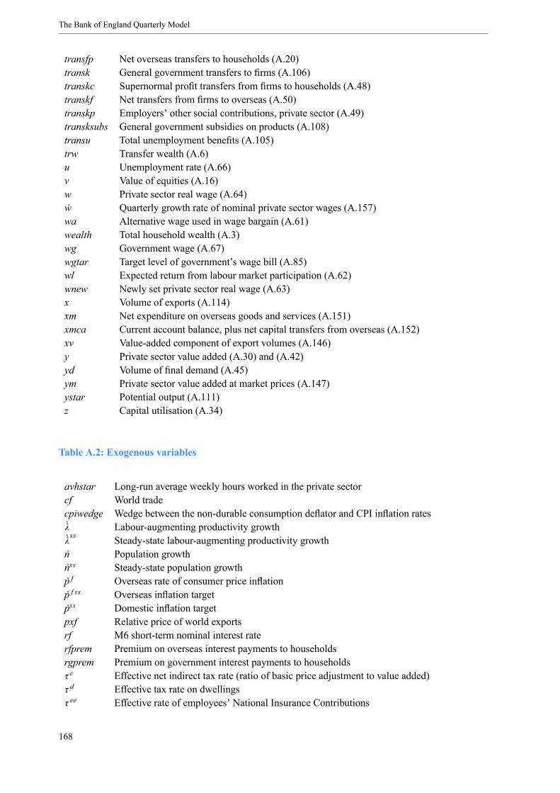
The Bank of England Quarterly Model
transfp Net overseas transfers to households (A.20)transk General government transfers to firms (A.106)transkc Supernormal profit transfers from firms to households (A.48)transkf Net transfers from firms to overseas (A.50)transkp Employers’ other social contributions, private sector (A.49)transksubs General government subsidies on products (A.108)transu Total unemployment benefits (A.105)trw Transfer wealth (A.6)u Unemployment rate (A.66)v Value of equities (A.16)w Private sector real wage (A.64)w Quarterly growth rate of nominal private sector wages (A.157)wa Alternative wage used in wage bargain (A.61)wealth Total household wealth (A.3)wg Government wage (A.67)wgtar Target level of government’s wage bill (A.85)wl Expected return from labour market participation (A.62)wnew Newly set private sector real wage (A.63)x Volume of exports (A.114)xm Net expenditure on overseas goods and services (A.151)xmca Current account balance, plus net capital transfers from overseas (A.152)xv Value-added component of export volumes (A.146)y Private sector value added (A.30) and (A.42)yd Volume of final demand (A.45)ym Private sector value added at market prices (A.147)ystar Potential output (A.111)z Capital utilisation (A.34)
Table A.2: Exogenous variables
avhstar Long-run average weekly hours worked in the private sectorcf World tradecpiwedge Wedge between the non-durable consumption deflator and CPI inflation ratesλ Labour-augmenting productivity growthλss Steady-state labour-augmenting productivity growthn Population growthnss Steady-state population growthp f Overseas rate of consumer price inflationp f ss Overseas inflation targetpss Domestic inflation targetpxf Relative price of world exportsrf M6 short-term nominal interest raterfprem Premium on overseas interest payments to householdsrgprem Premium on government interest payments to householdsτ c Effective net indirect tax rate (ratio of basic price adjustment to value added)τ d Effective tax rate on dwellingsτ ee Effective rate of employees’ National Insurance Contributions
168
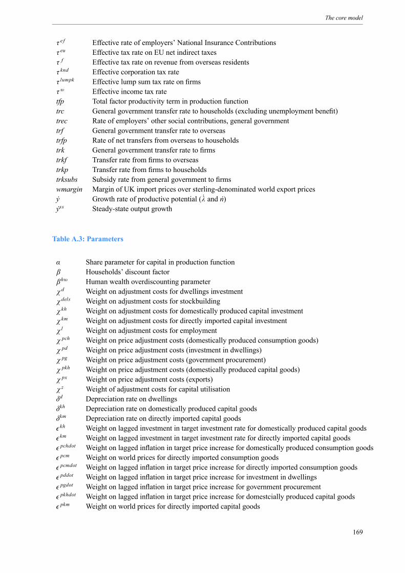
The core model
τ e f Effective rate of employers’ National Insurance Contributionsτ eu Effective tax rate on EU net indirect taxesτ f Effective tax rate on revenue from overseas residentsτ knd Effective corporation tax rateτ lumpk Effective lump sum tax rate on firmsτw Effective income tax ratetfp Total factor productivity term in production functiontrc General government transfer rate to households (excluding unemployment benefit)trec Rate of employers’ other social contributions, general governmenttrf General government transfer rate to overseastrfp Rate of net transfers from overseas to householdstrk General government transfer rate to firmstrkf Transfer rate from firms to overseastrkp Transfer rate from firms to householdstrksubs Subsidy rate from general government to firmswmargin Margin of UK import prices over sterling-denominated world export pricesy Growth rate of productive potential (λ and n)yss Steady-state output growth
Table A.3: Parameters
α Share parameter for capital in production functionβ Households’ discount factorβhw Human wealth overdiscounting parameterχd Weight on adjustment costs for dwellings investmentχdels Weight on adjustment costs for stockbuildingχ kh Weight on adjustment costs for domestically produced capital investmentχ km Weight on adjustment costs for directly imported capital investmentχ l Weight on adjustment costs for employmentχ pch Weight on price adjustment costs (domestically produced consumption goods)χ pd Weight on price adjustment costs (investment in dwellings)χ pg Weight on price adjustment costs (government procurement)χ pkh Weight on price adjustment costs (domestically produced capital goods)χ px Weight on price adjustment costs (exports)χ z Weight of adjustment costs for capital utilisationδd Depreciation rate on dwellingsδkh Depreciation rate on domestically produced capital goodsδkm Depreciation rate on directly imported capital goodskh Weight on lagged investment in target investment rate for domestically produced capital goodskm Weight on lagged investment in target investment rate for directly imported capital goodspchdot Weight on lagged inflation in target price increase for domestically produced consumption goodspcm Weight on world prices for directly imported consumption goodspcmdot Weight on lagged inflation in target price increase for directly imported consumption goodspddot Weight on lagged inflation in target price increase for investment in dwellingspgdot Weight on lagged inflation in target price increase for government procurementpkhdot Weight on lagged inflation in target price increase for domestcially produced capital goodspkm Weight on world prices for directly imported capital goods
169
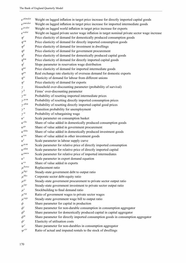
The Bank of England Quarterly Model
pkmdot Weight on lagged inflation in target price increase for directly imported capital goodspmidot Weight on lagged inflation in target price increase for imported intermediate goodspxdot Weight on lagged world inflation in target price increase for exportswdot Weight on lagged private sector wage inflation in target nominal private sector wage increaseηc Price elasticity of demand for domestically produced consumption goodsηcm Price elasticity of demand for directly imported consumption goodsηd Price elasticity of demand for investment in dwellingsηg Price elasticity of demand for government procurementηk Price elasticity of demand for domestically produced capital goodsηkm Price elasticity of demand for directly imported capital goodsηl Slope parameter in reservation wage distributionηmi Price elasticity of demand for imported intermediate goodsηpx Real exchange rate elasticity of overseas demand for domestic exportsηw Elasticity of demand for labour from different unionsηx Price elasticity of demand for exportsγ Household over-discounting parameter (probability of survival)γ k Firms’ over-discounting parameterγ mi Probability of resetting imported intermediate pricesγ pcm Probability of resetting directly imported consumption pricesγ pkm Probability of resetting directly imported capital good pricesγ u Transition probability for unemploymentγ w Probability of rebargaining wageκc Scale parameter on consumption basketκchv Share of value added in domestically produced consumption goodsκgv Share of value added in government procurementκ ikhv Share of value added in domestically produced investment goodsκ iov Share of value added in other investment goodsκ l Scale parameter in labour supply curveκ pcm Scale parameter for relative price of directly imported consumptionκ pkm Scale parameter for relative price of directly imported capitalκ pmin Scale parameter for relative price of imported intermediatesκ x Scale parameter in export demand equationκ xv Share of value added in exportsµbenw Replacement ratioµbgy Steady-state government debt to output ratioµbkv Corporate sector debt-equity ratioµgy Steady-state government procurement to private sector output ratioµigy Steady-state government investment to private sector output ratioµs Stockbuilding to final demand ratioµwg Ratio of government wages to private sector wagesµwgy Steady-state government wage bill to output ratioφ Share parameter for capital in productionφc Share parameter for non-durable consumption in consumption aggregatorφk Share parameter for domestically produced capital in capital aggregatorφm Share parameter for directly imported consumption goods in consumption aggregatorφz Elasticity of utilisation costsψc Share parameter for non-durables in consumption aggregatorψcir Ratio of actual and imputed rentals to the stock of dwellings
170
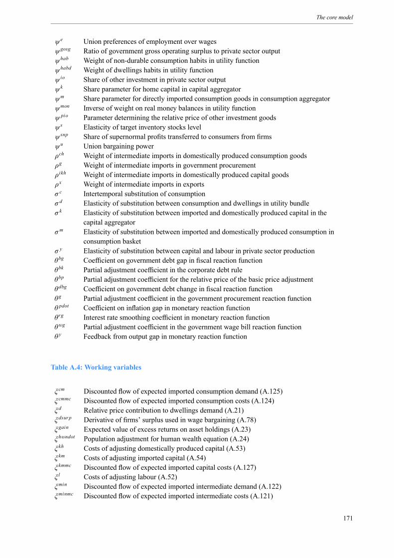
The core model
ψe Union preferences of employment over wagesψgosg Ratio of government gross operating surplus to private sector outputψhab Weight of non-durable consumption habits in utility functionψhabd Weight of dwellings habits in utility functionψ io Share of other investment in private sector outputψk Share parameter for home capital in capital aggregatorψm Share parameter for directly imported consumption goods in consumption aggregatorψmon Inverse of weight on real money balances in utility functionψ pio Parameter determining the relative price of other investment goodsψ s Elasticity of target inventory stocks levelψ snp Share of supernormal profits transferred to consumers from firmsψu Union bargaining powerρch Weight of intermediate imports in domestically produced consumption goodsρg Weight of intermediate imports in government procurementρikh Weight of intermediate imports in domestically produced capital goodsρx Weight of intermediate imports in exportsσ c Intertemporal substitution of consumptionσ d Elasticity of substitution between consumption and dwellings in utility bundleσ k Elasticity of substitution between imported and domestically produced capital in the
capital aggregatorσm Elasticity of substitution between imported and domestically produced consumption in
consumption basketσ y Elasticity of substitution between capital and labour in private sector productionθbg Coefficient on government debt gap in fiscal reaction functionθbk Partial adjustment coefficient in the corporate debt ruleθbp Partial adjustment coefficient for the relative price of the basic price adjustmentθdbg Coefficient on government debt change in fiscal reaction functionθ g Partial adjustment coefficient in the government procurement reaction functionθ pdot Coefficient on inflation gap in monetary reaction functionθ rg Interest rate smoothing coefficient in monetary reaction functionθwg Partial adjustment coefficient in the government wage bill reaction functionθ y Feedback from output gap in monetary reaction function
Table A.4: Working variables
ξ cm Discounted flow of expected imported consumption demand (A.125)ξ cmmc Discounted flow of expected imported consumption costs (A.124)ξ d Relative price contribution to dwellings demand (A.21)ξ dsurp Derivative of firms’ surplus used in wage bargaining (A.78)ξ gain Expected value of excess returns on asset holdings (A.23)ξ hwndot Population adjustment for human wealth equation (A.24)ξ kh Costs of adjusting domestically produced capital (A.53)ξ km Costs of adjusting imported capital (A.54)ξ kmmc Discounted flow of expected imported capital costs (A.127)ξ l Costs of adjusting labour (A.52)ξmin Discounted flow of expected imported intermediate demand (A.122)ξminmc Discounted flow of expected imported intermediate costs (A.121)
171
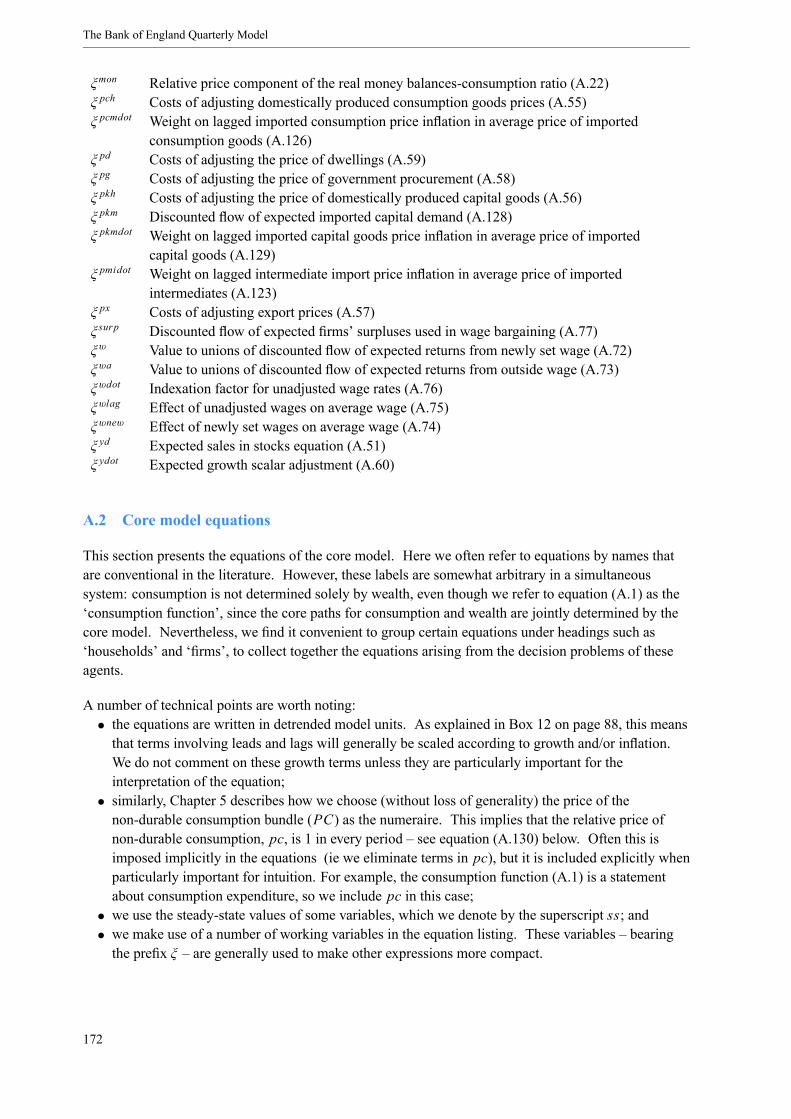
The Bank of England Quarterly Model
ξmon Relative price component of the real money balances-consumption ratio (A.22)ξ pch Costs of adjusting domestically produced consumption goods prices (A.55)ξ pcmdot Weight on lagged imported consumption price inflation in average price of imported
consumption goods (A.126)ξ pd Costs of adjusting the price of dwellings (A.59)ξ pg Costs of adjusting the price of government procurement (A.58)ξ pkh Costs of adjusting the price of domestically produced capital goods (A.56)ξ pkm Discounted flow of expected imported capital demand (A.128)ξ pkmdot Weight on lagged imported capital goods price inflation in average price of imported
capital goods (A.129)ξ pmidot Weight on lagged intermediate import price inflation in average price of imported
intermediates (A.123)ξ px Costs of adjusting export prices (A.57)ξ surp Discounted flow of expected firms’ surpluses used in wage bargaining (A.77)ξw Value to unions of discounted flow of expected returns from newly set wage (A.72)ξwa Value to unions of discounted flow of expected returns from outside wage (A.73)ξwdot Indexation factor for unadjusted wage rates (A.76)ξwlag Effect of unadjusted wages on average wage (A.75)ξwnew Effect of newly set wages on average wage (A.74)ξ yd Expected sales in stocks equation (A.51)ξ ydot Expected growth scalar adjustment (A.60)
A.2 Core model equations
This section presents the equations of the core model. Here we often refer to equations by names thatare conventional in the literature. However, these labels are somewhat arbitrary in a simultaneoussystem: consumption is not determined solely by wealth, even though we refer to equation (A.1) as the‘consumption function’, since the core paths for consumption and wealth are jointly determined by thecore model. Nevertheless, we find it convenient to group certain equations under headings such as‘households’ and ‘firms’, to collect together the equations arising from the decision problems of theseagents.
A number of technical points are worth noting:• the equations are written in detrended model units. As explained in Box 12 on page 88, this meansthat terms involving leads and lags will generally be scaled according to growth and/or inflation.We do not comment on these growth terms unless they are particularly important for theinterpretation of the equation;
• similarly, Chapter 5 describes how we choose (without loss of generality) the price of thenon-durable consumption bundle (PC) as the numeraire. This implies that the relative price ofnon-durable consumption, pc, is 1 in every period – see equation (A.130) below. Often this isimposed implicitly in the equations (ie we eliminate terms in pc), but it is included explicitly whenparticularly important for intuition. For example, the consumption function (A.1) is a statementabout consumption expenditure, so we include pc in this case;
• we use the steady-state values of some variables, which we denote by the superscript ss; and• we make use of a number of working variables in the equation listing. These variables – bearingthe prefix ξ – are generally used to make other expressions more compact.
172
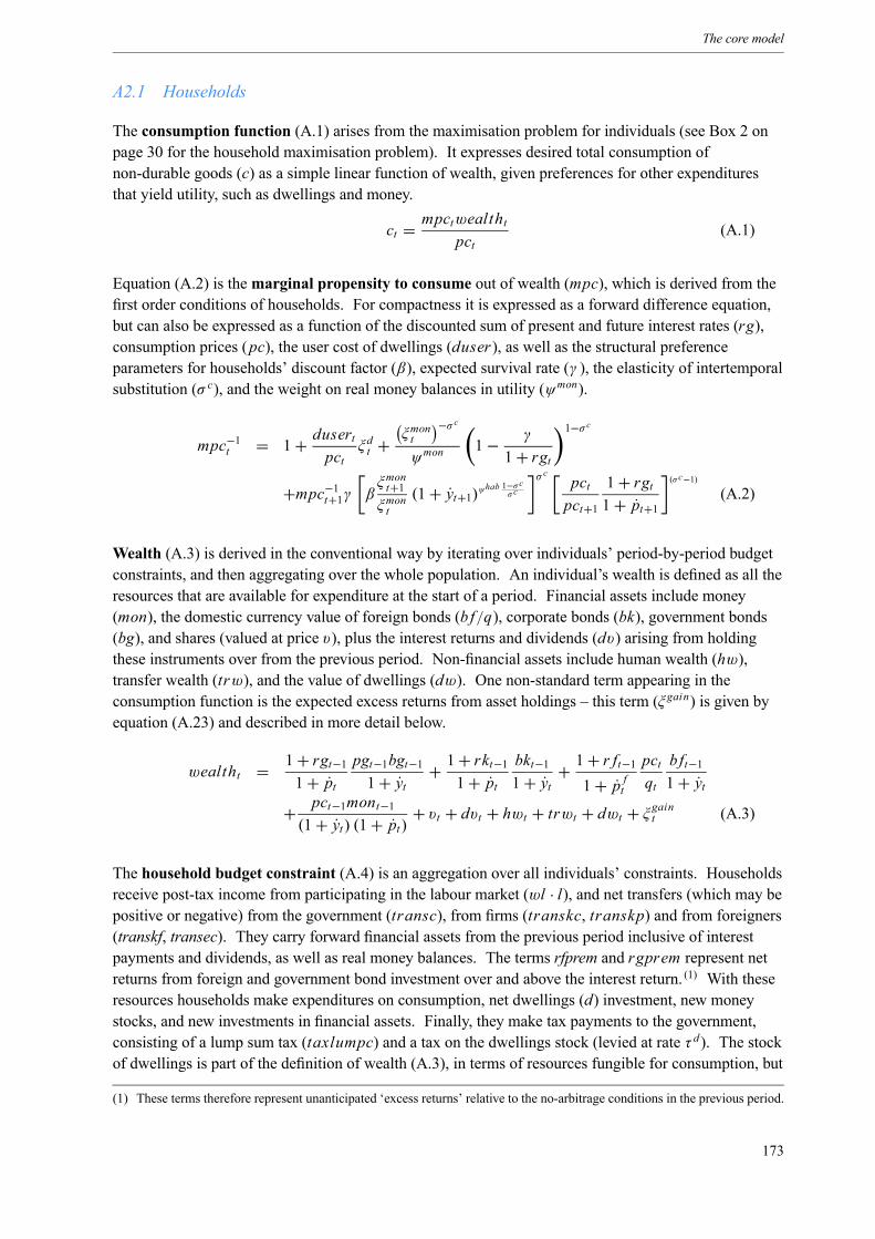
The core model
A2.1 Households
The consumption function (A.1) arises from the maximisation problem for individuals (see Box 2 onpage 30 for the household maximisation problem). It expresses desired total consumption ofnon-durable goods (c) as a simple linear function of wealth, given preferences for other expendituresthat yield utility, such as dwellings and money.
ct = mpctwealthtpct(A.1)
Equation (A.2) is themarginal propensity to consume out of wealth (mpc), which is derived from thefirst order conditions of households. For compactness it is expressed as a forward difference equation,but can also be expressed as a function of the discounted sum of present and future interest rates (rg),consumption prices (pc), the user cost of dwellings (duser), as well as the structural preferenceparameters for households’ discount factor (β), expected survival rate (γ ), the elasticity of intertemporalsubstitution (σ c), and the weight on real money balances in utility (ψmon).
mpc−1t = 1+ dusertpct
ξ dt +ξmont
−σ c
ψmon1− γ
1+ rgt1−σ c
+mpc−1t+1γ βξmont+1ξmont
(1+ yt+1)ψhab 1−σc
σc
σ c pctpct+1
1+ rgt1+ pt+1
(σc−1)(A.2)
Wealth (A.3) is derived in the conventional way by iterating over individuals’ period-by-period budgetconstraints, and then aggregating over the whole population. An individual’s wealth is defined as all theresources that are available for expenditure at the start of a period. Financial assets include money(mon), the domestic currency value of foreign bonds (b f/q), corporate bonds (bk), government bonds(bg), and shares (valued at price v), plus the interest returns and dividends (dv) arising from holdingthese instruments over from the previous period. Non-financial assets include human wealth (hw),transfer wealth (trw), and the value of dwellings (dw). One non-standard term appearing in theconsumption function is the expected excess returns from asset holdings – this term (ξ gain) is given byequation (A.23) and described in more detail below.
wealtht = 1+ rgt−11+ pt
pgt−1bgt−11+ yt + 1+ rkt−1
1+ ptbkt−11+ yt +
1+ r ft−11+ p ft
pctqtb ft−11+ yt
+ pct−1mont−1(1+ yt) (1+ pt) + vt + dvt + hwt + trwt + dwt + ξ
gaint (A.3)
The household budget constraint (A.4) is an aggregation over all individuals’ constraints. Householdsreceive post-tax income from participating in the labour market (wl · l), and net transfers (which may bepositive or negative) from the government (transc), from firms (transkc, transkp) and from foreigners(transkf, transec). They carry forward financial assets from the previous period inclusive of interestpayments and dividends, as well as real money balances. The terms rfprem and rgprem represent netreturns from foreign and government bond investment over and above the interest return. (1) With theseresources households make expenditures on consumption, net dwellings (d) investment, new moneystocks, and new investments in financial assets. Finally, they make tax payments to the government,consisting of a lump sum tax (taxlumpc) and a tax on the dwellings stock (levied at rate τ d). The stockof dwellings is part of the definition of wealth (A.3), in terms of resources fungible for consumption, but
(1) These terms therefore represent unanticipated ‘excess returns’ relative to the no-arbitrage conditions in the previous period.
173
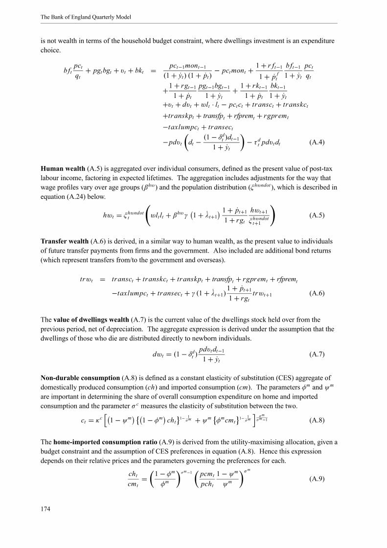
The Bank of England Quarterly Model
is not wealth in terms of the household budget constraint, where dwellings investment is an expenditurechoice.
b ftpctqt+ pgtbgt + vt + bkt = pct−1mont−1
(1+ yt) (1+ pt) − pctmont +1+ r ft−11+ p ft
b ft−11+ yt
pctqt
+1+ rgt−11+ pt
pgt−1bgt−11+ yt + 1+ rkt−1
1+ ptbkt−11+ yt
+vt + dvt +wlt · lt − pctct + transct + transkct+transkpt + transfpt + rfpremt + rgpremt−taxlumpct + transect−pdvt dt − (1− δ
dt )dt−1
1+ yt − τ dt pdvt dt (A.4)
Human wealth (A.5) is aggregated over individual consumers, defined as the present value of post-taxlabour income, factoring in expected lifetimes. The aggregation includes adjustments for the way thatwage profiles vary over age groups (βhw) and the population distribution (ξ hwndot ), which is described inequation (A.24) below.
hwt = ξ hwndott wlt lt + βhwγ 1+ λt+1 1+ pt+11+ rgthwt+1ξ hwndott+1
(A.5)
Transfer wealth (A.6) is derived, in a similar way to human wealth, as the present value to individualsof future transfer payments from firms and the government. Also included are additional bond returns(which represent transfers from/to the government and overseas).
trwt = transct + transkct + transkpt + transfpt + rgpremt + rfpremt−taxlumpct + transect + γ (1+ λt+1)1+ pt+11+ rgt trwt+1 (A.6)
The value of dwellings wealth (A.7) is the current value of the dwellings stock held over from theprevious period, net of depreciation. The aggregate expression is derived under the assumption that thedwellings of those who die are distributed directly to newborn individuals.
dwt = (1− δdt )pdvt dt−11+ yt (A.7)
Non-durable consumption (A.8) is defined as a constant elasticity of substitution (CES) aggregate ofdomestically produced consumption (ch) and imported consumption (cm). The parameters φm and ψm
are important in determining the share of overall consumption expenditure on home and importedconsumption and the parameter σ c measures the elasticity of substitution between the two.
ct = κc 1− ψm 1− φm cht 1− 1σm + ψm φmcmt 1− 1
σmσmσm−1 (A.8)
The home-imported consumption ratio (A.9) is derived from the utility-maximising allocation, given abudget constraint and the assumption of CES preferences in equation (A.8). Hence this expressiondepends on their relative prices and the parameters governing the preferences for each.
chtcmt
= 1− φmφm
σm−1 pcmtpcht
1− ψmψm
σm
(A.9)
174
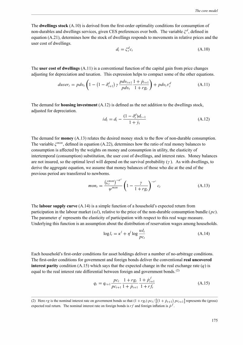
The core model
The dwellings stock (A.10) is derived from the first-order optimality conditions for consumption ofnon-durables and dwellings services, given CES preferences over both. The variable ξ d , defined inequation (A.21), determines how the stock of dwellings responds to movements in relative prices and theuser cost of dwellings.
dt = ξ dt ct (A.10)
The user cost of dwellings (A.11) is a conventional function of the capital gain from price changesadjusting for depreciation and taxation. This expression helps to compact some of the other equations.
dusert = pdvt 1− 1− δdt+1 γpdvt+1pdvt
1+ pt+11+ rgt + pdvtτ dt (A.11)
The demand for housing investment (A.12) is defined as the net addition to the dwellings stock,adjusted for depreciation.
idt = dt − (1− δdt )dt−1
1+ yt (A.12)
The demand formoney (A.13) relates the desired money stock to the flow of non-durable consumption.The variable ξmon, defined in equation (A.22), determines how the ratio of real money balances toconsumption is affected by the weights on money and consumption in utility, the elasticity ofintertemporal (consumption) substitution, the user cost of dwellings, and interest rates. Money balancesare not insured, so the optimal level will depend on the survival probability (γ ). As with dwellings, toderive the aggregate equation, we assume that money balances of those who die at the end of theprevious period are transferred to newborns.
mont = ξmont−σ c
ψmon1− γ
1+ rgt−σcct (A.13)
The labour supply curve (A.14) is a simple function of a household’s expected return fromparticipation in the labour market (wl), relative to the price of the non-durable consumption bundle (pc).The parameter ηl represents the elasticity of participation with respect to this real wage measure.Underlying this function is an assumption about the distribution of reservation wages among households.
log lt = κ l + ηl log wltpct (A.14)
Each household’s first-order conditions for asset holdings deliver a number of no-arbitrage conditions.The first-order conditions for government and foreign bonds deliver the conventional real uncoveredinterest parity condition (A.15) which says that the expected change in the real exchange rate (q) isequal to the real interest rate differential between foreign and government bonds. (2)
qt = qt+1 pctpct+11+ rgt1+ pt+1
1+ p ft+11+ r ft (A.15)
(2) Here rg is the nominal interest rate on government bonds so that (1+ rgt ) pct/ 1+ pt+1 pct+1 represents the (gross)expected real return. The nominal interest rate on foreign bonds is r f and foreign inflation is p f .
175
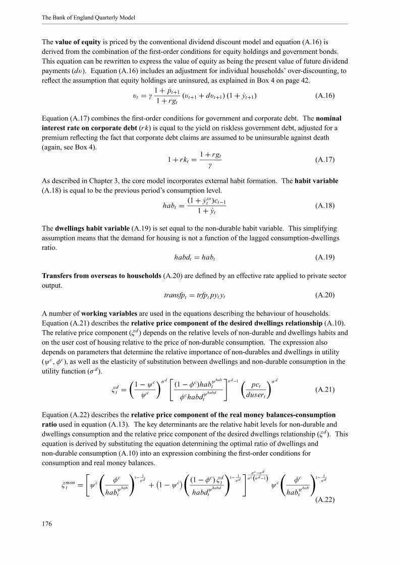
The Bank of England Quarterly Model
The value of equity is priced by the conventional dividend discount model and equation (A.16) isderived from the combination of the first-order conditions for equity holdings and government bonds.This equation can be rewritten to express the value of equity as being the present value of future dividendpayments (dv). Equation (A.16) includes an adjustment for individual households’ over-discounting, toreflect the assumption that equity holdings are uninsured, as explained in Box 4 on page 42.
vt = γ 1+ pt+11+ rgt (vt+1 + dvt+1) (1+ yt+1) (A.16)
Equation (A.17) combines the first-order conditions for government and corporate debt. The nominalinterest rate on corporate debt (rk) is equal to the yield on riskless government debt, adjusted for apremium reflecting the fact that corporate debt claims are assumed to be uninsurable against death(again, see Box 4).
1+ rkt = 1+ rgtγ
(A.17)
As described in Chapter 3, the core model incorporates external habit formation. The habit variable(A.18) is equal to be the previous period’s consumption level.
habt = (1+ ysst )ct−1
1+ yt (A.18)
The dwellings habit variable (A.19) is set equal to the non-durable habit variable. This simplifyingassumption means that the demand for housing is not a function of the lagged consumption-dwellingsratio.
habdt = habt (A.19)
Transfers from overseas to households (A.20) are defined by an effective rate applied to private sectoroutput.
transfpt = trfpt pyt yt (A.20)
A number of working variables are used in the equations describing the behaviour of households.Equation (A.21) describes the relative price component of the desired dwellings relationship (A.10).The relative price component (ξ d) depends on the relative levels of non-durable and dwellings habits andon the user cost of housing relative to the price of non-durable consumption. The expression alsodepends on parameters that determine the relative importance of non-durables and dwellings in utility(ψc, φc), as well as the elasticity of substitution between dwellings and non-durable consumption in theutility function (σ d).
ξ dt =1− ψcψc
σ d (1− φc)habψhabt
φchabdψhabd
t
σd−1 pctdusert
σ d
(A.21)
Equation (A.22) describes the relative price component of the real money balances-consumptionratio used in equation (A.13). The key determinants are the relative habit levels for non-durable anddwellings consumption and the relative price component of the desired dwellings relationship (ξ d). Thisequation is derived by substituting the equation determining the optimal ratio of dwellings andnon-durable consumption (A.10) into an expression combining the first-order conditions forconsumption and real money balances.
ξmont = ψcφc
habψhab
t
1− 1σd + 1− ψc (1− φc) ξ dt
habdψhabd
t
1− 1σd
σ c−σdσc(σd−1)
ψcφc
habψhab
t
1− 1σd
(A.22)
176
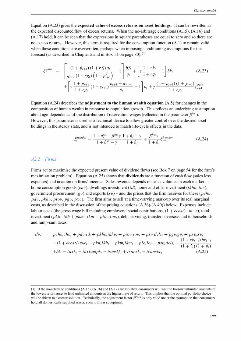
The core model
Equation (A.23) gives the expected value of excess returns on asset holdings. It can be rewritten asthe expected discounted flow of excess returns. When the no-arbitrage conditions (A.15), (A.16) and(A.17) hold, it can be seen that the expressions in square parentheses are equal to zero and so there areno excess returns. However, this term is required for the consumption function (A.1) to remain validwhen these conditions are overwritten, perhaps when imposing conditioning assumptions for theforecast (as described in Chapter 5 and in Box 11 on page 80). (3)
ξgaint =
⎡⎣ (1+ pt+1) (1+ r ft) qtqt+1 (1+ rgt) 1+ p ft+1
− 1⎤⎦ b ftqt+ γ
1+ rkt1+ rgt − 1 bkt (A.23)
+ γ1+ pt+11+ rgt (1+ yt+1)
vt+1 + dvt+1vt
− 1 vt + γ (1+ pt+1) (1+ yt+1)1+ rgt ξgaint+1
Equation (A.24) describes the adjustment to the human wealth equation (A.5) for changes in thecomposition of human wealth in response to population growth. This reflects an underlying assumptionabout age-dependence of the distribution of reservation wages (reflected in the parameter βhw).However, this parameter is used as a technical device to allow greater control over the desired assetholdings in the steady state, and is not intended to match life-cycle effects in the data.
ξ hwndott = 1+ nsst − βhwγ
1+ nsst − γ1+ nt − γ1+ nt + βhwγ
1+ nt ξhwndott−1 (A.24)
A2.2 Firms
Firms act to maximise the expected present value of dividend flows (see Box 7 on page 54 for the firm’smaximisation problem). Equation (A.25) shows that dividends are a function of cash flow (sales lessexpenses) and taxation on firms’ income. Sales revenue depends on sales volumes in each market –home consumption goods (chv), dwellings investment (id), home and other investment (ikhv , iov),government procurement (gv) and exports (xv) – and the prices that the firm receives for these (pchv ,pdv , pkhv , piov , pgv , pxv). The firm aims to sell at a time-varying mark-up over its real marginalcosts, as described in the discussion of the pricing equations (A.36)-(A.40)) below. Expenses includelabour costs (the gross wage bill including employers’ social contributions, (1+ ecost) · w · e), totalinvestment (pkh · ikh + pkm · ikm + piovt iovt ), debt servicing, transfers overseas and to households,and lump-sum taxes.
dvt = pchvt chvt + pdvt idt + pkhvt ikhvt + piovt iovt + psvt delst + pgvt gvt + pxvt xvt− (1+ ecostt)wt et − pkht ikht − pkmtikmt − piot iot − psvt delst − (1+ rkt−1) bkt−1
(1+ yt) (1+ pt)+bkt − taxkt − taxlumpkt − transkf t + transkt − transkct (A.25)
(3) If the no-arbitrage conditions (A.15), (A.16) and (A.17) are violated, consumers will want to borrow unlimited amounts ofthe lowest return asset to lend unlimited amounts at the highest rate of return. This implies that the optimal portfolio choicewill be driven to a corner solution. Technically, the adjustment factor ξgain is only valid under the assumption that consumershold all domestically supplied assets, even if this is suboptimal.
177
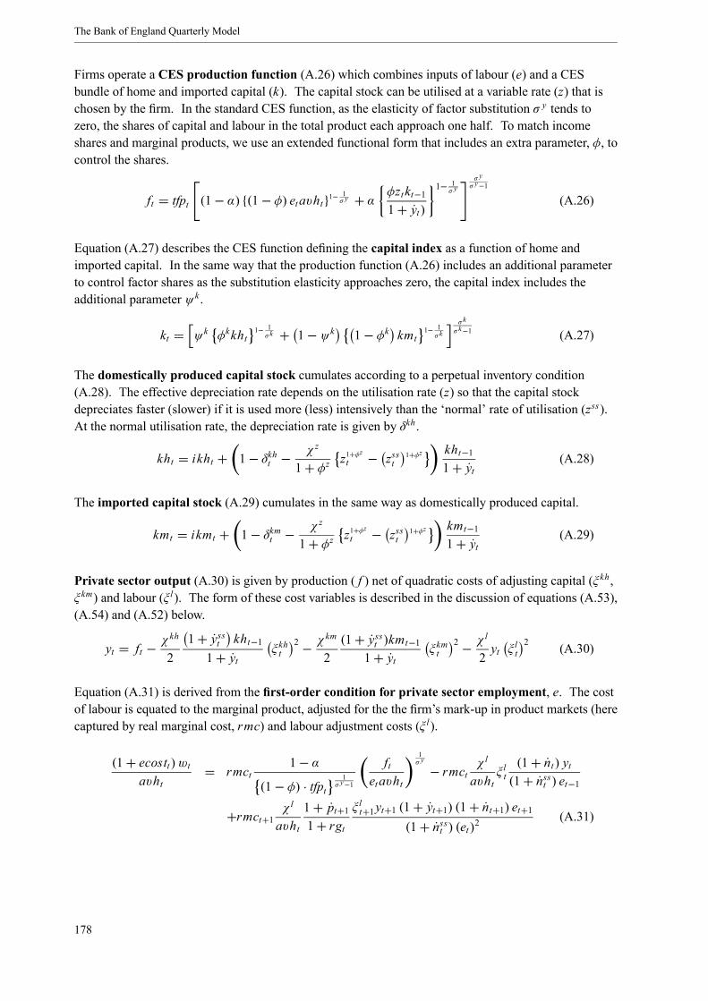
The Bank of England Quarterly Model
Firms operate a CES production function (A.26) which combines inputs of labour (e) and a CESbundle of home and imported capital (k). The capital stock can be utilised at a variable rate (z) that ischosen by the firm. In the standard CES function, as the elasticity of factor substitution σ y tends tozero, the shares of capital and labour in the total product each approach one half. To match incomeshares and marginal products, we use an extended functional form that includes an extra parameter, φ, tocontrol the shares.
ft = tfpt (1− α) {(1− φ) etavht}1− 1σ y + α φztkt−1
1+ yt)1− 1
σ yσ yσ y−1
(A.26)
Equation (A.27) describes the CES function defining the capital index as a function of home andimported capital. In the same way that the production function (A.26) includes an additional parameterto control factor shares as the substitution elasticity approaches zero, the capital index includes theadditional parameter ψk .
kt = ψk φkkht1− 1σk + 1− ψk 1− φk kmt 1− 1
σkσkσ k−1 (A.27)
The domestically produced capital stock cumulates according to a perpetual inventory condition(A.28). The effective depreciation rate depends on the utilisation rate (z) so that the capital stockdepreciates faster (slower) if it is used more (less) intensively than the ‘normal’ rate of utilisation (zss).At the normal utilisation rate, the depreciation rate is given by δkh .
kht = ikht + 1− δkht −χ z
1+ φz z1+φzt − zsst1+φz kht−1
1+ yt (A.28)
The imported capital stock (A.29) cumulates in the same way as domestically produced capital.
kmt = ikmt + 1− δkmt − χ z
1+ φz z1+φzt − zsst1+φz kmt−1
1+ yt (A.29)
Private sector output (A.30) is given by production ( f ) net of quadratic costs of adjusting capital (ξ kh ,ξ km) and labour (ξ l). The form of these cost variables is described in the discussion of equations (A.53),(A.54) and (A.52) below.
yt = ft − χkh
21+ ysst kht−11+ yt ξ kht
2 − χkm
2(1+ ysst )kmt−1
1+ yt ξ kmt2 − χ
l
2yt ξ lt
2 (A.30)
Equation (A.31) is derived from the first-order condition for private sector employment, e. The costof labour is equated to the marginal product, adjusted for the the firm’s mark-up in product markets (herecaptured by real marginal cost, rmc) and labour adjustment costs (ξ l).
(1+ ecostt)wtavht
= rmct1− α
(1− φ) · tfpt1
σ y−1
ftetavht
1σ y − rmct χ
l
avhtξ lt(1+ nt) yt(1+ nsst ) et−1
+rmct+1 χl
avht1+ pt+11+ rgt
ξ lt+1yt+1 (1+ yt+1) (1+ nt+1) et+1(1+ nsst ) (et)2
(A.31)
178
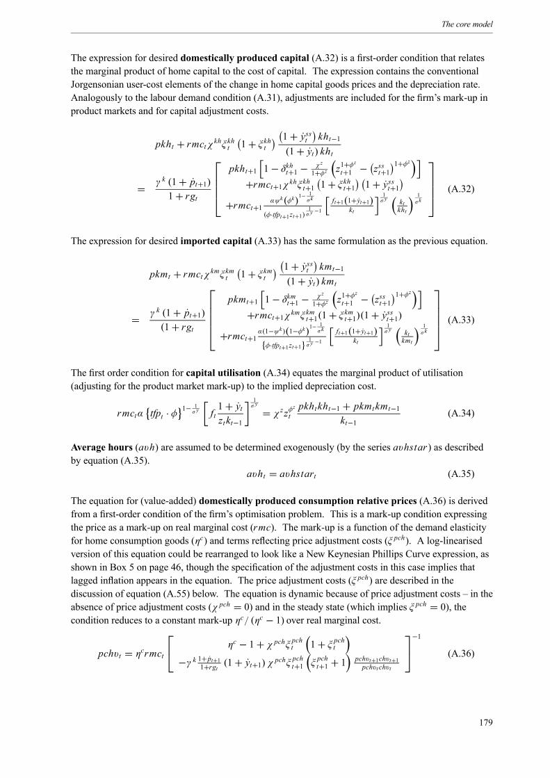
The core model
The expression for desired domestically produced capital (A.32) is a first-order condition that relatesthe marginal product of home capital to the cost of capital. The expression contains the conventionalJorgensonian user-cost elements of the change in home capital goods prices and the depreciation rate.Analogously to the labour demand condition (A.31), adjustments are included for the firm’s mark-up inproduct markets and for capital adjustment costs.
pkht + rmctχ khξ kht 1+ ξ kht1+ ysst kht−1(1+ yt) kht
= γ k (1+ pt+1)1+ rgt
⎡⎢⎢⎢⎣pkht+1 1− δkht+1 − χ z
1+φz z1+φz
t+1 − zsst+11+φz
+rmct+1χ khξ kht+1 1+ ξ kht+1 1+ ysst+1+rmct+1 αψk(φk)
1− 1σk
(φ·tfpt+1zt+1)1σ y −1
ft+1(1+yt+1)kt
1σ y kt
kht
1σk
⎤⎥⎥⎥⎦ (A.32)
The expression for desired imported capital (A.33) has the same formulation as the previous equation.
pkmt + rmctχ kmξ kmt 1+ ξ kmt1+ ysst kmt−1(1+ yt) kmt
= γ k (1+ pt+1)(1+ rgt
⎡⎢⎢⎢⎢⎣pkmt+1 1− δkmt+1 − χ z
1+φz z1+φz
t+1 − zsst+11+φz
+rmct+1χ kmξ kmt+1(1+ ξ kmt+1)(1+ ysst+1)+rmct+1 α(1−ψ
k )(1−φk)1−1σk
{φ·tfpt+1zt+1} 1σ y −1ft+1(1+yt+1)
kt
1σ y kt
kmt
1σk
⎤⎥⎥⎥⎥⎦ (A.33)
The first order condition for capital utilisation (A.34) equates the marginal product of utilisation(adjusting for the product market mark-up) to the implied depreciation cost.
rmctα tfpt · φ 1− 1σ y ft
1+ ytzt kt−1
1σ y = χ zzφzt pkhtkht−1 + pkmtkmt−1kt−1
(A.34)
Average hours (avh) are assumed to be determined exogenously (by the series avhstar) as describedby equation (A.35).
avht = avhstart (A.35)
The equation for (value-added) domestically produced consumption relative prices (A.36) is derivedfrom a first-order condition of the firm’s optimisation problem. This is a mark-up condition expressingthe price as a mark-up on real marginal cost (rmc). The mark-up is a function of the demand elasticityfor home consumption goods (ηc) and terms reflecting price adjustment costs (ξ pch). A log-linearisedversion of this equation could be rearranged to look like a New Keynesian Phillips Curve expression, asshown in Box 5 on page 46, though the specification of the adjustment costs in this case implies thatlagged inflation appears in the equation. The price adjustment costs (ξ pch) are described in thediscussion of equation (A.55) below. The equation is dynamic because of price adjustment costs – in theabsence of price adjustment costs (χ pch = 0) and in the steady state (which implies ξ pch = 0), thecondition reduces to a constant mark-up ηc/ (ηc − 1) over real marginal cost.
pchvt = ηcrmct⎡⎣ ηc − 1+ χ pchξ pcht 1+ ξ pcht−γ k 1+ pt+11+rgt (1+ yt+1) χ pchξ
pcht+1 ξ
pcht+1 + 1 pchvt+1chvt+1
pchvt chvt
⎤⎦−1 (A.36)
179
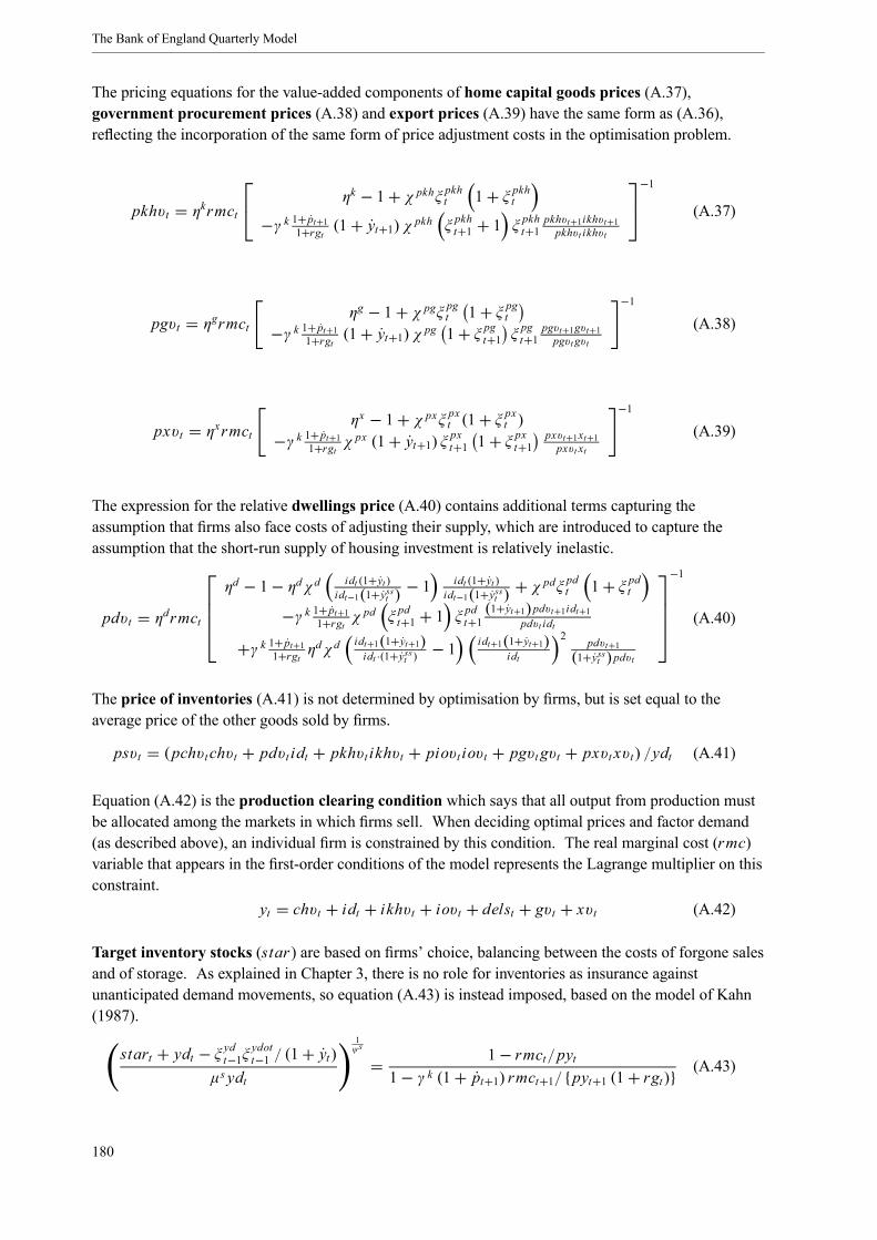
The Bank of England Quarterly Model
The pricing equations for the value-added components of home capital goods prices (A.37),government procurement prices (A.38) and export prices (A.39) have the same form as (A.36),reflecting the incorporation of the same form of price adjustment costs in the optimisation problem.
pkhvt = ηkrmct⎡⎣ ηk − 1+ χ pkhξ pkht 1+ ξ pkht−γ k 1+ pt+11+rgt (1+ yt+1) χ pkh ξ
pkht+1 + 1 ξ
pkht+1
pkhvt+1ikhvt+1pkhvt ikhvt
⎤⎦−1 (A.37)
pgvt = ηgrmct ηg − 1+ χ pgξ pgt 1+ ξ pgt−γ k 1+ pt+11+rgt (1+ yt+1) χ pg 1+ ξ
pgt+1 ξ
pgt+1
pgvt+1gvt+1pgvt gvt
−1(A.38)
pxvt = ηxrmct ηx − 1+ χ pxξ pxt (1+ ξ pxt )−γ k 1+ pt+11+rgt χ
px (1+ yt+1) ξ pxt+1 1+ ξ pxt+1 pxvt+1xt+1pxvt xt
−1(A.39)
The expression for the relative dwellings price (A.40) contains additional terms capturing theassumption that firms also face costs of adjusting their supply, which are introduced to capture theassumption that the short-run supply of housing investment is relatively inelastic.
pdvt = ηdrmct
⎡⎢⎢⎢⎣ηd − 1− ηdχd idt (1+yt )
idt−1(1+ysst ) − 1idt (1+yt )
idt−1(1+ysst ) + χpdξ
pdt 1+ ξ pdt
−γ k 1+ pt+11+rgt χpd ξ
pdt+1 + 1 ξ
pdt+1(1+yt+1)pdvt+1idt+1
pdvt idt
+γ k 1+ pt+11+rgt ηdχd
idt+1(1+yt+1)idt ·(1+ysst ) − 1 idt+1(1+yt+1)
idt
2 pdvt+1(1+ysst )pdvt
⎤⎥⎥⎥⎦−1
(A.40)
The price of inventories (A.41) is not determined by optimisation by firms, but is set equal to theaverage price of the other goods sold by firms.
psvt = (pchvt chvt + pdvt idt + pkhvt ikhvt + piovt iovt + pgvt gvt + pxvt xvt) /ydt (A.41)
Equation (A.42) is the production clearing condition which says that all output from production mustbe allocated among the markets in which firms sell. When deciding optimal prices and factor demand(as described above), an individual firm is constrained by this condition. The real marginal cost (rmc)variable that appears in the first-order conditions of the model represents the Lagrange multiplier on thisconstraint.
yt = chvt + idt + ikhvt + iovt + delst + gvt + xvt (A.42)
Target inventory stocks (star) are based on firms’ choice, balancing between the costs of forgone salesand of storage. As explained in Chapter 3, there is no role for inventories as insurance againstunanticipated demand movements, so equation (A.43) is instead imposed, based on the model of Kahn(1987).
start + ydt − ξ ydt−1ξ ydott−1 / (1+ yt)µs ydt
1ψs
= 1− rmct/pyt1− γ k (1+ pt+1) rmct+1/ {pyt+1 (1+ rgt)} (A.43)
180
The core model
The level of actual inventories (s) is generally not at the target level in each period and equation (A.44)describes the determination of inventory stocks given quadratic costs of adjustment. The parameterχdels measures the size of adjustment costs (so that setting χdels = 0 implies that inventories are alwaysat target).
st 1+ χdels + χdels 1+ pt+11+ rgt 1+ ysst = start + 1+ pt+11+ rgt (1+ yt+1) χdelsst+1
+χdelsst−1 1+ ysst
1+ yt (A.44)
The level of private sector demand excluding stockbuilding is given by equation (A.45).
ydt = chvt + idt + ikhvt + iovt + gvt + xvt (A.45)
The rate of change of stocks – stockbuilding (dels) – is defined by the identity (A.46).
delst = st − st−11+ yt (A.46)
Corporate debt issuance (A.47) is imposed to avoid ‘corner solutions’ in which the firm is financedentirely by either debt or equity. We assume that the stock of corporate bonds depends on the value ofequity and the level of bonds in the previous period.
bkt = 1− θbk µbkvvt + θbkbkt−1 (A.47)
Supernormal profit transfers from firms to consumers (A.48) are given by a proportion (ψ snp) of thevalue of private sector output.
transkct = ψ snp pyt yt (A.48)
Employers’ (other) private social contributions to households (A.49) are given by the application of atransfer weight (trkp) to the pre-tax private sector wage bill.
transkpt = trkpt · wt et (A.49)
Transfers from firms to overseas are defined by equation (A.50).
transkf t = trkf t · pyt yt (A.50)
We now turn to the working variables that appear in the firms’ equations. The desired stock level –star described in equation (A.43) – depends on the lagged expectation of demand (excludingstockbuilding) one period ahead (A.51), the model-consistent solution for the level prevailing nextperiod, absent any shocks.
ξydt = ydt+1 (A.51)
The labour adjustment cost (A.52) is defined as the net change in employment.
ξ lt =(1+ nt) et(1+ nsst ) et−1 − 1 (A.52)
181
The Bank of England Quarterly Model
The domestically produced capital adjustment cost (A.53) is a function of the net and lagged changesin the home capital stock. The parameter kh determines the extent to which lagged changes in thecapital stock affect adjustment costs. When kh = 0 capital adjustment costs depend only on the changein the capital stock, but when 0 < kh < 1 the lagged change in the capital stock also matter foradjustment costs. This specification means that the first order condition for home capital can depend onlagged investment and is similar to the specification of external habit formation in consumption.
ξ kht =(1+ yt) kht/kht−1
(1+ ysst )1− kh {kht−1 (1+ yt−1) /kht−2} kh− 1 (A.53)
The imported capital adjustment cost (A.54) is defined analogously to the cost for home capital – as afunction of the net and lagged changes in the imported capital stock.
ξ kmt = (1+ yt) kmt/kmt−1(1+ ysst )1− km
(kmt−1 (1+ yt−1) /kmt−2) km− 1 (A.54)
The cost of adjusting domestically produced consumption prices (A.55) has the same form as thecapital adjustment costs of equations (A.53) and (A.54). The cost depends on the deviation betweennominal home consumption price inflation ((1+ pt) pchvt/pchvt−1) and a weighted average ofsteady-state inflation and lagged home consumption price inflation. The parameter pchdot controls theweighting. When pchdot = 0, the pricing equation (A.36) can be log-linearised to deliver a NewKeynesian Phillips curve representation in a very similar way to the example in Box 5 on page 46.When pchdot takes a value between 0 and 1, the log-linearised relationship also contains a term inlagged home consumption price inflation.
ξpcht = (1+ pt) pchvt/pchvt−1
(1+ psst )1− pchdot((1+ pt−1) pchvt−1/pchvt−2) pchdot − 1 (A.55)
The cost of adjusting domestically produced capital goods prices (A.56) has the same form as theequation for ξ pch .
ξpkht = (1+ pt) pkhvt/pkhvt−1
(1+ psst )1− pkhdot((1+ pt−1) pkhvt−1/pkhvt−2) pkhdot − 1 (A.56)
The cost of adjusting export prices (A.57) has a similar form, though two differences are important.First, the adjustment cost is defined in terms of the foreign currency price of export goods, reflecting theassumption that exporters set their prices in foreign currency. Second, when px takes a value between 0and 1, the lagged price inflation that matters is world export price inflation (in foreign currency). Thisreflects the assumption that exporters respond to pricing developments in world markets.
ξpxt =
1+ p ft pxvtqt/ (pxvt−1qt−1)
1+ p f sst1− pxdot
1+ p ft−1 pxf t−1/pxf t−2pxdot − 1 (A.57)
The costs of adjusting prices of government procurement (A.58) and dwellings prices (A.59) havethe same form as the equation for ξ pch .
ξpgt = (1+ pt) pgvt/pgvt−1
(1+ psst )1− pgdot((1+ pt−1) pgvt−1/pgvt−2) pgdot − 1 (A.58)
ξpdt = (1+ pt) pdvt/pdvt−1
(1+ psst )1− pddot((1+ pt−1) pdvt−1/pdvt−2) pddot − 1 (A.59)
182
The core model
The desired stock level – star described in equation (A.43) – depends on the lagged expectation ofsupply growth one-period ahead (A.60), which is the model-consistent solution for the level prevailingnext period, absent any shocks.
ξydott = 1+ yt+1 (A.60)
A2.3 Wage bargaining
Wage bargaining takes place to maximise a Nash maximand of firms’ and unions’ surpluses – see Box 8on page 58 for a description of the optimisation problem. The outside wage (A.61) is a weightedaverage of the post-tax wages from (private and public sector) employment and unemployment benefit.The weights are related to the unemployment rate (u), the rate of employment in the public sector (µeg)and a parameter (γ u) that summarises the likelihood of unemployed workers re-entering the pool ofavailable labour.
wat = 1− γ uut − γ uµegt 1− τwt − τ eet wt + γ uutbent + γ uµegt 1− τwt − τ eet wgt (A.61)
Equation (A.62) shows that the expected wage from participation is a weighted average of the post-taxwages from (private and public sector) employment and unemployment benefit. The weights are givenby the rates of employment (in private and public sectors) and unemployment respectively. When theparameter γ u = 1 in equation (A.61), then wa = wl.
wlt = 1− ut − µegt 1− τwt − τ eet wt + utbent + µegt 1− τwt − τ eet wgt (A.62)
The first-order condition for the wage bargain (A.63) determines the equilibrium real wage. Theexpression is derived from the equilibrium condition of the Nash bargain and equates the marginalbenefit to unions of an increase in the wage rate (left-hand side of the expression) to the marginal cost tofirms of that increase (right-hand side). In a static framework, the marginal benefit would be anincreasing function of the difference between the bargained wage and the outside alternative. Given thatnominal wage contracts are negotiated infrequently, the marginal benefit depends on the expectedevolution of the difference between ξwt and ξ
watt and this also explains the extensive use of working
variables. The marginal cost to firms is a function of the expected evolution of labour costs relative torevenues.
ψu(1− ηwψe) ξwt + ηwψeξwat
ξwt − ξwat= − 1− ψu ξ
dsurpt
ξsurpt
(A.63)
The average wage is a weighted average of newly set wages and unadjusted wages. Equation (A.64)transforms this relationship using working variables described below – see equations (A.74) and (A.75).Newly set wages (on which ξwnew depends) arise out of the wage bargain; unadjusted wages (on whichξwlag depends) are assumed to be indexed by a weighted average of steady-state and past nominal wageinflation. The weight on newly set wages, γ w, is the Calvo adjustment probability (the probability thatwages are reset in any given period). When γ w = 1 nominal wages are perfectly flexible and newly setand average wages coincide.
1 = γ wξwnewt + (1− γ w) ξwlagt (A.64)
183
The Bank of England Quarterly Model
The theoretical structure of the core model assumes that total employment is an index overheterogeneous labour types (each represented by a union – see Box 8 on page 58). Equation (A.65)shows how this index is related to private sector employment. The Calvo adjustment probability playsa role here as well, when; γ w = 1 (flexible nominal wages) the employment index and the private sectoremployment rate will coincide.
ent = γ w wnewtwt
−ηwet + (1− γ w) etet−1
wt (1+ pt) 1+ λtξwdott wt−1
ηw
ent−1 (A.65)
The unemployment rate (A.66) measures the proportion of the participating labour force (l) notemployed in the private sector (en) or public sector (eg).
ut = lt − ent − egtlt(A.66)
The public sector wage (A.67) is related to the private sector wage according to the factor µwg.
wgt = µwgwt (A.67)
The share of public sector employment in participation (A.68) is defined as:
µegt = egtlt (A.68)
The firm’s surplus (A.69), over which the wage bargain is made, is defined as sales revenue less wagecosts. The definition of the firm’s surplus is somewhat open, but equation (A.69) is a standardassumption that also prevents transfers influencing the wage bargain, which would be the case, say, ifdividends were used as the measure of surplus.
surpt = pchvt chvt + pdvt idt + pkhvt ikhvt + piovt iovt + psvtdelst+gvt pgvt + pxvt xvt − (1+ ecostt)wt et (A.69)
We assume that unemployment benefits (A.70) are an exogenous fraction of the private sector realwage. So µbenw represents the replacement ratio. This implies that unemployment benefit grows in linewith wages (and hence labour productivity). (This is a requirement in the long run, so that the naturalrate of unemployment does not exhibit a trend, but we need not assume this in the short run.)
bent = µbenwwt (A.70)
The labour input (A.71) into production is measured in hours with a simple equation converting theemployment index into hours.
eht = etavht (A.71)
Turning to working variables, as noted in the discussion of equation (A.63), the bargained real wagedepends on the expected benefits to unions from negotiating the newly set wage. The expectedmarginal benefit to unions of the newly set wage is given by equation (A.72), which shows that thisbenefit depends on the expected flow of future post-tax wages and employment levels. When nominalwages are completely flexible (γ w = 1) the second (dynamic) term disappears.
184
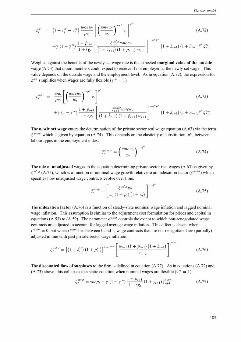
The core model
ξwt = 1− τwt − τ eetwnewtpct
wnewtwt
−ηwet
ψe
(A.72)
+γ (1− γ w) 1+ pt+11+ rgt
ξwdott+1 wnewt1+ λt+1 (1+ pt+1)wt+1
1−ψeηw
1+ λt+1 (1+ nt+1)ψe ξwt+1
Weighed against the benefits of the newly set wage rate is the expectedmarginal value of the outsidewage (A.73) that union members could expect to receive if not employed at the newly set wage. Thisvalue depends on the outside wage and the employment level. As in equation (A.72), the expression forξwa simplifies when wages are fully flexible (γ w = 1).
ξwat = watpct
wnewtwt
−ηwet
ψe
(A.73)
+γ (1− γ w) 1+ pt+11+ rgt
ξwdott+1 wnewt1+ λt+1 (1+ pt+1)wt+1
−ηwψe
1+ λt+1 (1+ nt+1)ψe ξwat+1
The newly set wage enters the determination of the private sector real wage equation (A.63) via the termξwnew which is given by equation (A.74). This depends on the elasticity of substitution, ηw, betweenlabour types in the employment index.
ξwnewt = wnewtwt
1−ηw(A.74)
The role of unadjusted wages in the equation determining private sector real wages (A.63) is given byξwlag (A.75), which is a function of nominal wage growth relative to an indexation factor (ξwdot ) whichspecifies how unadjusted wage contracts evolve over time.
ξwlagt = ξwdott wt−1
wt (1+ pt) 1+ λt
1−ηw
(A.75)
The indexation factor (A.76) is a function of steady-state nominal wage inflation and lagged nominalwage inflation. This assumption is similar to the adjustment cost formulation for prices and capital inequations (A.53) to (A.59). The parameter wdot controls the extent to which non-renegotiated wagecontracts are adjusted to account for lagged average wage inflation. This effect is absent whenwdot = 0, but when wdot lies between 0 and 1, wage contracts that are not renegotiated are (partially)adjusted in line with past private sector wage inflation.
ξwdott = 1+ λsst 1+ psst 1− wdot wt−1 (1+ pt−1) 1+ λt−1wt−2
wdot
(A.76)
The discounted flow of surpluses to the firm is defined in equation (A.77). As in equations (A.72) and(A.73) above, this collapses to a static equation when nominal wages are flexible (γ w = 1).
ξsurpt = surpt + γ (1− γ w) 1+ pt+11+ rgt (1+ yt+1) ξ
surpt+1 (A.77)
185
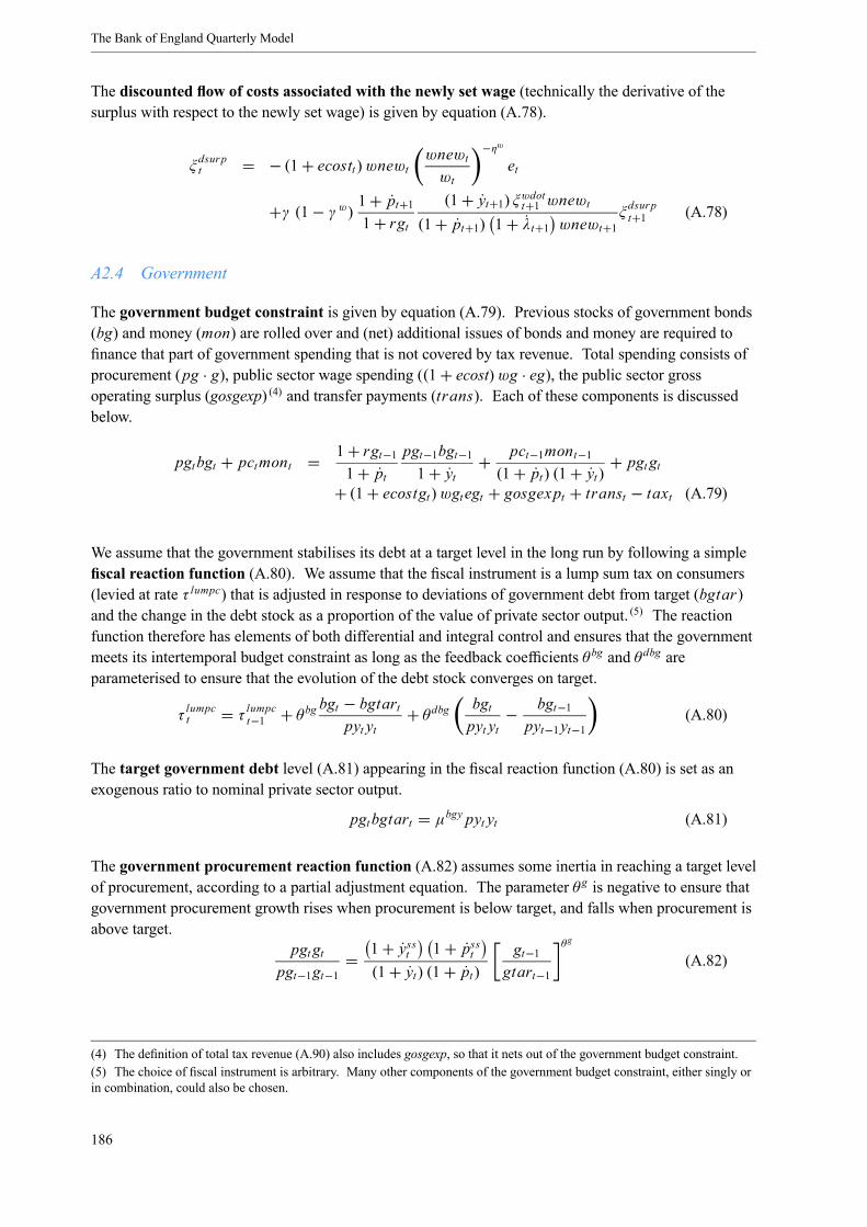
The Bank of England Quarterly Model
The discounted flow of costs associated with the newly set wage (technically the derivative of thesurplus with respect to the newly set wage) is given by equation (A.78).
ξdsurpt = − (1+ ecostt)wnewt wnewt
wt
−ηwet
+γ (1− γ w) 1+ pt+11+ rgt
(1+ yt+1) ξwdott+1 wnewt(1+ pt+1) 1+ λt+1 wnewt+1 ξ
dsurpt+1 (A.78)
A2.4 Government
The government budget constraint is given by equation (A.79). Previous stocks of government bonds(bg) and money (mon) are rolled over and (net) additional issues of bonds and money are required tofinance that part of government spending that is not covered by tax revenue. Total spending consists ofprocurement (pg · g), public sector wage spending ((1+ ecost) wg · eg), the public sector grossoperating surplus (gosgexp) (4) and transfer payments (trans). Each of these components is discussedbelow.
pgtbgt + pctmont = 1+ rgt−11+ pt
pgt−1bgt−11+ yt + pct−1mont−1
(1+ pt) (1+ yt) + pgt gt+ (1+ ecostgt)wgtegt + gosgexpt + transt − taxt (A.79)
We assume that the government stabilises its debt at a target level in the long run by following a simplefiscal reaction function (A.80). We assume that the fiscal instrument is a lump sum tax on consumers(levied at rate τ lumpc) that is adjusted in response to deviations of government debt from target (bgtar)and the change in the debt stock as a proportion of the value of private sector output. (5) The reactionfunction therefore has elements of both differential and integral control and ensures that the governmentmeets its intertemporal budget constraint as long as the feedback coefficients θbg and θdbg areparameterised to ensure that the evolution of the debt stock converges on target.
τlumpct = τ lumpct−1 + θbg bgt − bgtart
pyt yt+ θdbg bgt
pyt yt− bgt−1pyt−1yt−1
(A.80)
The target government debt level (A.81) appearing in the fiscal reaction function (A.80) is set as anexogenous ratio to nominal private sector output.
pgtbgtart = µbgy pyt yt (A.81)
The government procurement reaction function (A.82) assumes some inertia in reaching a target levelof procurement, according to a partial adjustment equation. The parameter θ g is negative to ensure thatgovernment procurement growth rises when procurement is below target, and falls when procurement isabove target.
pgt gtpgt−1gt−1
= 1+ ysst 1+ psst(1+ yt) (1+ pt)
gt−1gtart−1
θ g
(A.82)
(4) The definition of total tax revenue (A.90) also includes gosgexp, so that it nets out of the government budget constraint.(5) The choice of fiscal instrument is arbitrary. Many other components of the government budget constraint, either singly orin combination, could also be chosen.
186
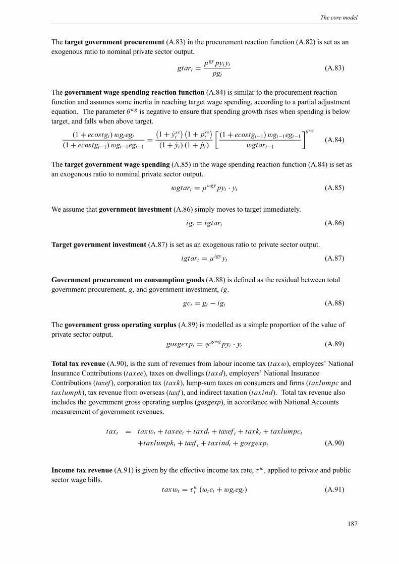
The core model
The target government procurement (A.83) in the procurement reaction function (A.82) is set as anexogenous ratio to nominal private sector output.
gtart = µgy pyt ytpgt
(A.83)
The government wage spending reaction function (A.84) is similar to the procurement reactionfunction and assumes some inertia in reaching target wage spending, according to a partial adjustmentequation. The parameter θwg is negative to ensure that spending growth rises when spending is belowtarget, and falls when above target.
(1+ ecostgt)wgtegt(1+ ecostgt−1) wgt−1egt−1 =
1+ ysst 1+ psst(1+ yt) (1+ pt)
(1+ ecostgt−1)wgt−1egt−1wgtart−1
θwg
(A.84)
The target government wage spending (A.85) in the wage spending reaction function (A.84) is set asan exogenous ratio to nominal private sector output.
wgtart = µwgy pyt · yt (A.85)
We assume that government investment (A.86) simply moves to target immediately.
igt = igtart (A.86)
Target government investment (A.87) is set as an exogenous ratio to private sector output.
igtart = µigy yt (A.87)
Government procurement on consumption goods (A.88) is defined as the residual between totalgovernment procurement, g, and government investment, ig.
gct = gt − igt (A.88)
The government gross operating surplus (A.89) is modelled as a simple proportion of the value ofprivate sector output.
gosgexpt = ψgosg pyt · yt (A.89)
Total tax revenue (A.90), is the sum of revenues from labour income tax (taxw), employees’ NationalInsurance Contributions (taxee), taxes on dwellings (taxd), employers’ National InsuranceContributions (taxef ), corporation tax (taxk), lump-sum taxes on consumers and firms (taxlumpc andtaxlumpk), tax revenue from overseas (taxf ), and indirect taxation (taxind). Total tax revenue alsoincludes the government gross operating surplus (gosgexp), in accordance with National Accountsmeasurement of government revenues.
taxt = taxwt + taxeet + taxdt + taxef t + taxkt + taxlumpct+taxlumpkt + taxf t + taxindt + gosgexpt (A.90)
Income tax revenue (A.91) is given by the effective income tax rate, τw, applied to private and publicsector wage bills.
taxwt = τwt (wt et +wgtegt) (A.91)
187
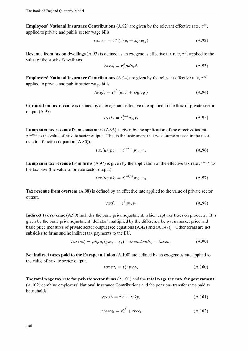
The Bank of England Quarterly Model
Employees’ National Insurance Contributions (A.92) are given by the relevant effective rate, τ ee,applied to private and public sector wage bills.
taxeet = τ eet (wt et +wgtegt) (A.92)
Revenue from tax on dwellings (A.93) is defined as an exogenous effective tax rate, τ d, applied to thevalue of the stock of dwellings.
taxdt = τ dt pdvtdt (A.93)
Employers’ National Insurance Contributions (A.94) are given by the relevant effective rate, τ e f ,applied to private and public sector wage bills.
taxef t = τ e ft (wt et +wgtegt) (A.94)
Corporation tax revenue is defined by an exogenous effective rate applied to the flow of private sectoroutput (A.95).
taxkt = τ kndt pyt yt (A.95)
Lump sum tax revenue from consumers (A.96) is given by the application of the effective tax rateτ lumpc to the value of private sector output. This is the instrument that we assume is used in the fiscalreaction function (equation (A.80)).
taxlumpct = τ lumpct pyt · yt (A.96)
Lump sum tax revenue from firms (A.97) is given by the application of the effective tax rate τ lumpk tothe tax base (the value of private sector output).
taxlumpkt = τ lumpkt pyt · yt (A.97)
Tax revenue from overseas (A.98) is defined by an effective rate applied to the value of private sectoroutput.
taxf t = τ ft pyt yt (A.98)
Indirect tax revenue (A.99) includes the basic price adjustment, which captures taxes on products. It isgiven by the basic price adjustment ‘deflator’ multiplied by the difference between market price andbasic price measures of private sector output (see equations (A.42) and (A.147)). Other terms are netsubsidies to firms and he indirect tax payments to the EU.
taxindt = pbpat (ymt − yt)+ transksubst − taxeut (A.99)
Net indirect taxes paid to the European Union (A.100) are defined by an exogenous rate applied tothe value of private sector output.
taxeut = τ eut pyt yt (A.100)
The total wage tax rate for private sector firms (A.101) and the total wage tax rate for government(A.102) combine employers’ National Insurance Contributions and the pensions transfer rates paid tohouseholds.
ecostt = τ e ft + trkpt (A.101)
ecostgt = τ e ft + trect (A.102)
188
The core model
Total transfer payments from government (A.103) consists of transfers to households (transc,rgprem), to the unemployed (ie benefits, transu), to firms (transk, transksubs) and overseas (transf ).
transt = transct + transut + transkt + transf t + transksubst + rgpremt (A.103)
Transfers to consumers (excluding unemployment benefits) (A.104) are defined by a rate applied tothe value of private sector output.
transct = trct pyt yt (A.104)
Total unemployment benefits (A.105) are defined by the rate from (A.70) applied to the number ofunemployed.
transut = bentutlt (A.105)
Government transfers to firms (A.106), transfers overseas (A.107), and transfer subsidies onproducts (A.108) are defined by a rate applied to the value of private sector output.
transkt = trkt pyt yt (A.106)
transf t = trf t pyt yt (A.107)
transksubst = trksubst pyt yt (A.108)
Social contributions paid to government employees (A.109) are defined by a rate applied to the valueof private sector output. They do not appear in the definition of total transfers (A.103) because they areincorporated in the government wage bill, through the definition of ecostg in equation (A.102).
transect = trectwgtegt (A.109)
A2.5 Monetary authority
The nominal side is anchored by amonetary reaction function (A.110). In the default setting, this is aTaylor-type rule where the short-term nominal rate is used as an instrument to ensure that inflationreturns to its target, psst .
rgt = 1− θ rg rgsst + θ pdot d4cpit − psst + θ y log yt + gltystart
+ θrgrgt−1 (A.110)
The reaction function responds to the deviations of a four-quarter inflation measure (d4cpi , defined inequation (A.138) below) from the inflation target pss and to a measure of output relative to potential.Potential output (A.111) is derived from the private sector production function using the steady-statelevels of total (i.e. private and public sector) employment and capital utilisation.
ystart = tfpt (1− α) (1− φ) 1− usst lsst avhsst
1− 1σ y + α φ
zsst kt−11+ yt
1− 1σ y
σ yσ y−1
(A.111)
189
The Bank of England Quarterly Model
The level of output entering the policy rule is given by private sector output (y) plus the governmentdemand for resources expressed in terms of private sector output. Equation (A.112) shows that this iscalculated by evaluating the private sector production function using actual total employment (e+ eg)and private capital when utilised at the steady-state rate (zss); and then subtracting the value of privatesector output that would be produced using only private sector employment and capital, when capitalutilisation is at its steady-state rate.
glt = tfpt (1− α) {(1− φ) (et + egt) avhstart}1− 1σ y + α φzsst kt−1
1+ yt1− 1
σ yσ yσ y−1
−tfpt (1− α) {(1− φ) etavhstart}1− 1σ y + α φzsst kt−1
1+ yt1− 1
σ yσ yσ y−1
(A.112)
A2.6 External
Imported intermediates (A.113) combine expenditure components where the ρ parameters denote theimported intermediate shares of individual expenditure components. As described in Chapter 3, finaloutput is produced by combining private sector output (produced by domestic firms), importedintermediate goods and tax payments to the government, using a Leontief technology. (6) The remainingimports into the economy are directly imported consumption (determined by the consumption index(A.8)) and directly imported investment (see equation (A.33)).
mit = ρchcht + ρikhikht + ρggt + ρx xt (A.113)
The demand for exports (A.114) is a conventional downward-sloping curve in the price of domesticexports relative to (exogenous) world export prices, pxf. The elasticity of demand is given by theparameter ηpx . World demand is given by the exogenous variable c f . Though we do not model thedecisions of agents in the rest of the world from first principles, the demand function (A.114) isconsistent with the assumption that consumers in the rest of the world allocate their consumption amongdomestically produced goods and goods produced in the rest of the world according to CES preferencessimilar to the ones specified for domestic consumers in equation (A.8).
xt = κ x pxtqtpxf t
−ηpxc ft (A.114)
The relative price of imported intermediate goods (A.115) is the average of newly set and unadjustedprices. The parameter γ mi is the Calvo price adjustment probability: imported intermediates goodsprices are adjusted with probability γ mi each period, and under perfectly flexible imported intermediateprices (γ mi = 1), the average price and newly set price coincide. Equations (A.116) and (A.117) showthat the relative prices of imported consumption goods and of imported capital goods are givenanalogously.
pmint =⎡⎣γ mi pminew1−ηmit + 1− γ mi ξ
pmidott pmint−11+ pt
1−ηmi⎤⎦1
1−ηmi
(A.115)
(6) Technically, the ρ parameters are the inverse of the imported intermediate coefficients in the Leontief technologies.
190
The core model
pcmt =⎡⎣γ pcm pcmnew1−ηcmt + 1− γ pcm ξ
pcmdott pcmt−11+ pt
1−ηcm⎤⎦ 11−ηcm
(A.116)
pkmt =⎡⎣γ pkm pkmnew1−ηkmt + 1− γ pkm ξ
pkmdott pkmt−11+ pt
1−ηkm⎤⎦1
1−ηkm
(A.117)
The newly set imported intermediate price (A.118) is a function of the expected discounted costs ofproduction (captured by ξminmc) relative to the expected discounted demand for the good (captured byξmin). (7) The newly set imported consumption price (A.119) and the newly set imported capitalprice (A.120) are given analogously. (8)
pminewt = pmint ξminmct
ξmint(A.118)
pcmnewt = pcmtξ cmmctξ cmt
(A.119)
pkmnewt = pkmt ξkmmct
ξpkmt
(A.120)
Turning to working variables, the expected flow of imported intermediate costs (A.121) shows thateach period the costs are given by the world price of exports in domestic currency (pxf /q) adjusted foran exogenous ‘margins effect’ (wmargin) and an exogenous scaling factor (κpmin). The margins effect isincluded because movements in measured world trade prices can have different effects on the worldprices of UK imports and of UK exports. The scaling factor reflects the fact that the price of importedintermediates may not be well captured by the world export price (since the imported intermediatebundle is likely to consist of different goods to the bundle of goods traded on world export markets).The expected flow is equal to the discounted sum of future costs, where the discount factor depends onthe Calvo adjustment probability γ mi .
ξminmct = mitκ pmin (1+wmargint) pxf t pctpmintqt
+ 1− γ mi 1+ pft
1+ r ftpmint+1 (1+ pt+1)pmintξ pmidott+1
ηmi+1ξminmct+1 (A.121)
The expected flow of imported intermediate demand (A.122) is equal to the expected discounted flowof imported intermediates. As before, the discount factor depends on the Calvo price adjustmentprobability γ mi .
ξmint = mit + 1− γ mi 1+ pft
1+ r ftpmint+1 (1+ pt+1)pmintξ pmidott+1
ηmi
ξmint+1 (A.122)
(7) These working variables are given by equations (A.121) and (A.122) below.(8) The relevant working variables are described by the pairs of equations (A.124)-(A.125) and (A.127)-(A.128) respectively.
191
The Bank of England Quarterly Model
We assume that for the duration of the pricing contract, unadjusted imported intermediates prices areincreased in line with an imported intermediates price indexation factor (A.123) that depends onsteady-state inflation and lagged imported intermediate price inflation. The parameter pmidot
determines the extent to which the indexation factor depends on lagged imported intermediate priceinflation.
ξpmidott = 1+ psst 1− pmidot (1+ pt−1) pmint−1
pmint−2
pmidot
(A.123)
The expected flow of imported consumption costs (A.124) has the same form as (A.121). However, inthis case, the cost may also depend on the price of domestic consumption goods. This is designed tocapture (in a non-structural way) the possibility that competition effects cause importers to interactstrategically with domestic producers, such that the import price is affected by the prices of domesticallyproduced goods. The extent of these effects is controlled by the parameter pcm .
ξ cmmct = cmt pcm · κ pcm (1+wmargint) pxf t pctpcmtqt+ 1− pcm · pcht
pcmt
+ 1− γ pcm 1+ p ft1+ r ft
pcmt+1 (1+ pt+1)pcmtξ pcmdott+1
ηcm+1ξ cmmct+1 (A.124)
The expected flow of imported consumption demand (A.125) is equal to the expected discounted flowof imported consumption. As before, the discount factor depends on the Calvo price adjustmentprobability γ pcm .
ξ cmt = cmt + 1− γ pcm 1+ p ft1+ r ft
pcmt+1 (1+ pt+1)pcmtξ pcmdott+1
ηcm
ξ cmt+1 (A.125)
Analogous to the treatment of imported intermediates prices, we assume that unadjusted importedconsumption prices are increased in line with an imported consumption price indexation factor(A.126).
ξpcmdott = 1+ psst 1− pcmdot (1+ pt−1) pcmt−1
pcmt−2
pcmdot
(A.126)
The expected flow of imported capital costs (A.127) is analogous to equation (A.124).
ξ kmmct = ikmt pkm · κ pkm(1+wmargint)pxf t pctpkmtqt+ (1− pkm) · pkht
pkmt
+ 1− γ pkm 1+ p ft1+ r ft
pkmt+1 (1+ pt+1)pkmtξ pkmdott+1
ηkm+1ξ kmmct+1 (A.127)
The expected flow of imported capital demand (A.128) is analogous to equation (A.125).
ξpkmt = ikmt + 1− γ pkm 1+ p ft
1+ r ftpkmt+1 (1+ pt+1)pkmtξ pkmdott+1
ηkm
ξpkmt+1 (A.128)
192
The core model
Analogous to the treatment of imported intermediate and imported consumption prices, we assume thatfor the duration of the pricing contract, unadjusted imported capital prices are increased in line with animported capital price indexation factor (A.129).
ξpkmdott = 1+ psst 1− pkmdot (1+ pt−1) pkmt−1
pkmt−2
pkmdot
(A.129)
A2.7 Prices and inflation
As explained in Chapter 5, the core model is written in stationary units, which requires a numeraire pricerelative to which all other prices are measured. Without loss of generality, we choose the non-durableconsumption price (excluding actual and imputed rents) to be the numeraire. By definition this meansthat the relative price of non-durable consumption (A.130) is equal to 1 in every period.
pct = 1 (A.130)
The relative price of non-durable consumption is also related to the (relative) prices of home andimported consumption by equation (A.131), which is simply the definition of total expenditure onconsumption (measured in detrended model units).
pctct = pcmtcmt + pchtcht (A.131)
The (relative) price of home consumption (A.132) is the weighted average of the prices of domesticallyproduced home consumption, imported intermediates and indirect taxes. (9) These relative prices aregiven by equations (A.36), (A.115) and (A.141) respectively.
pcht = κchv pchvt + ρch pmint + 1− κchv − ρch pbpat (A.132)
Equation (A.133) for the relative price of home capital is analogous to the expression for the relativemarket price of home consumption.
pkht = κ ikhv pkhvt + ρikh pmint + 1− κ ikhv − ρikh pbpat (A.133)
The relative price of other investment (A.137), has no imported intermediate component, so the price isa weighted average of the relative price of domestically produced other investment and the componentfor the basic price adjustment.
piot = κ iov piovt + 1− κ iov pbpat (A.134)
The relative price of government procurement (A.135) and themarket price of exports (A.136) areanalogous to the relative market price of home consumption.
pgt = κgv pgvt + ρg pmint + 1− κgv − ρg pbpat (A.135)
pxt = κ xv pxvt + ρx pmint + 1− κ xv − ρx pbpat (A.136)
The (relative) basic price of other investment (A.137) is not modelled as part of the firm’s optimalpricing decision but is instead linked by a simple equation to the basic price of home consumption.
piovt = ψ pio pchvt (A.137)
(9) The weights correspond to the (inverse) coefficients of the Leontief technology (discussed above) that combines domesticvalue added, imported intermediates and the basic price adjustment.
193
The Bank of England Quarterly Model
The four-quarter change in the CPI (A.138) is approximated by the four-quarter change in the price ofnon-durable consumption with an (exogenous) adjustment for the historical wedge between these series.This measure abstracts from seasonal effects.
d4cpit = 0.253
i=0( pt−i − cpiwedget−i ) (A.138)
Themarket price of private sector output (A.139) is given by the value of marketed output, measuredat market prices and adjusted for imported intermediates, divided by the volume of private sector outputat market prices, ym.
pymt ymt = pchtcht + pdvt idt + pkht ikht + piot iot + psvt delst+pgt gt + pxt xt − pmintmit (A.139)
The basic price of private sector output (A.140) is defined by subtracting the value of the basic priceadjustment from the market value of private production. This gives the basic price value of privatesector output which can then be divided by private sector output to calculate the price.
pyt yt = pymt ymt − pbpat (ymt − yt) (A.140)
The relative price of the basic price adjustment (A.141) depends on its own lag and the exogenous taxrate τ c, applied to the ratio of the basic price value of private sector output and the basic priceadjustment (ym − y). The parameter θbp controls the influence of the lag. When θbp = 0, the price issuch that the tax revenue from the basic price adjustment (representing taxes on products) is a fractionτ c of the (basic price) value of private sector output.
pbpat = θbp pbpat−1 + 1− θbp τ ctpyt yt
ymt − yt (A.141)
A2.8 Quantities
The (basic price) value-added component of domestically produced consumption (A.142) is derivedfrom the assumption that domestic value added, imported intermediates and basic price adjustment arecombined to produce final output using a Leontief technology, so there is a simple linear relationshipbetween the value-added quantity of home consumption and final home consumption. The parametercontrolling this relationship, κchv , appears in the underlying Leontief technology.
chvt = κchvcht (A.142)
The (basic price) value-added components of home investment (A.143), other investment (A.144),government procurement (A.145) and exports (A.146) are treated in the same way as homeconsumption.
ikhvt = κ ikhv ikht (A.143)
iovt = κ iov iot (A.144)
194
The core model
gvt = κgvgt (A.145)
xvt = κ xvxt (A.146)
The level of private sector output measured at market prices (A.147) adds the basic price adjustmentto basic price private sector output.
ymt = yt + 1− κchv − ρch cht + 1− κ ikhv − ρikh ikht + 1− κ iov iot+ 1− κgv − ρg gt + 1− κ xv − ρx xt (A.147)
Imputed and actual rents (A.148) are not modelled as part of the household optimisation problem andare defined as a simple function of the dwellings stock.
cirt = ψcirdt (A.148)
Other investment (A.33) is not modelled as part of the firm’s optimisation problem and is defined as asimple function of private sector output.
iot = ψ io yt (A.149)
A2.9 Accounting and reporting
We list here a number of variables that are not required for the solution of the core model but that arealso calculated.
Net foreign assets (A.150) are calculated as the domestic currency value of foreign bonds.
nfat =pctb ftqt
(A.150)
The value of the trade balance (A.151) is the value of exports less the value of total imports .
xmt = pxt xt − pcmtcmt − ikmt pkmt − pmintmit (A.151)
The value of the current account (A.152) is the trade balance plus net taxes and transfers overseas andinterest payments on the stock of net foreign assets.
xmcat = xmt + taxf t − transf t − transkf t + transfpt − taxeut+rfpremt +
r ft−1nfat−1(1+ pt) (1+ yt) (A.152)
Inflation rates (A.153) to (A.156) for the value-added price of home consumption, importedintermediates prices, the market price of home consumption and imported consumption prices aredefined as the change in the relative price multiplied by the inflation rate of the numeraire.
1+ pchvt = (1+ pt) pchvtpchvt−1
(A.153)
195
The Bank of England Quarterly Model
1+ pmint = (1+ pt) pmintpmint−1
(A.154)
1+ pcht =(1+ pt) pchtpcht−1
(A.155)
1+ pcmt = (1+ pt) pcmtpcmt−1
(A.156)
Nominal private sector wage inflation (A.157) is calculated as the change in the real wage multipliedby the numeraire inflation rate and the change in labour productivity.
1+ wt = (1+ pt) 1+ λt wtwt−1
(A.157)
Total asset holdings (A.158) includes the values of equities corporate bonds, government bonds, realmoney balances and net foreign assets.
at = vt + bkt + pgtbgt + pctmont + nfat (A.158)
A simple measure of total consumption (A.159) is given by the sum of home and importedconsumption.
cmodt = cmt + cht (A.159)
A simple measure of total investment (A.160) is given by the sum of home and imported investment.
ikt = ikht + ikmt (A.160)
196
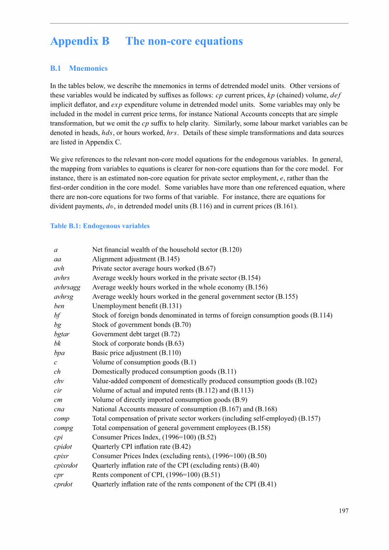
Appendix B The non-core equations
B.1 Mnemonics
In the tables below, we describe the mnemonics in terms of detrended model units. Other versions ofthese variables would be indicated by suffixes as follows: cp current prices, kp (chained) volume, de fimplicit deflator, and exp expenditure volume in detrended model units. Some variables may only beincluded in the model in current price terms, for instance National Accounts concepts that are simpletransformation, but we omit the cp suffix to help clarity. Similarly, some labour market variables can bedenoted in heads, hds, or hours worked, hrs. Details of these simple transformations and data sourcesare listed in Appendix C.
We give references to the relevant non-core model equations for the endogenous variables. In general,the mapping from variables to equations is clearer for non-core equations than for the core model. Forinstance, there is an estimated non-core equation for private sector employment, e, rather than thefirst-order condition in the core model. Some variables have more than one referenced equation, wherethere are non-core equations for two forms of that variable. For instance, there are equations fordivident payments, dv , in detrended model units (B.116) and in current prices (B.161).
Table B.1: Endogenous variables
a Net financial wealth of the household sector (B.120)aa Alignment adjustment (B.145)avh Private sector average hours worked (B.67)avhrs Average weekly hours worked in the private sector (B.154)avhrsagg Average weekly hours worked in the whole economy (B.156)avhrsg Average weekly hours worked in the general government sector (B.155)ben Unemployment benefit (B.131)bf Stock of foreign bonds denominated in terms of foreign consumption goods (B.114)bg Stock of government bonds (B.70)bgtar Government debt target (B.72)bk Stock of corporate bonds (B.63)bpa Basic price adjustment (B.110)c Volume of consumption goods (B.1)ch Domestically produced consumption goods (B.11)chv Value-added component of domestically produced consumption goods (B.102)cir Volume of actual and imputed rents (B.112) and (B.113)cm Volume of directly imported consumption goods (B.9)cna National Accounts measure of consumption (B.167) and (B.168)comp Total compensation of private sector workers (including self-employed) (B.157)compg Total compensation of general government employees (B.158)cpi Consumer Prices Index, (1996=100) (B.52)cpidot Quarterly CPI inflation rate (B.42)cpixr Consumer Prices Index (excluding rents), (1996=100) (B.50)cpixrdot Quarterly inflation rate of the CPI (excluding rents) (B.40)cpr Rents component of CPI, (1996=100) (B.51)cprdot Quarterly inflation rate of the rents component of the CPI (B.41)
197
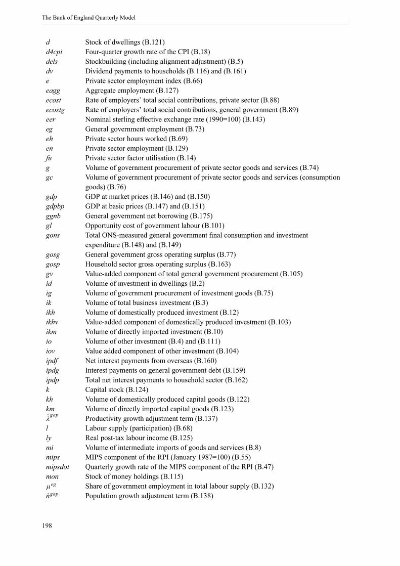
The Bank of England Quarterly Model
d Stock of dwellings (B.121)d4cpi Four-quarter growth rate of the CPI (B.18)dels Stockbuilding (including alignment adjustment) (B.5)dv Dividend payments to households (B.116) and (B.161)e Private sector employment index (B.66)eagg Aggregate employment (B.127)ecost Rate of employers’ total social contributions, private sector (B.88)ecostg Rate of employers’ total social contributions, general government (B.89)eer Nominal sterling effective exchange rate (1990=100) (B.143)eg General government employment (B.73)eh Private sector hours worked (B.69)en Private sector employment (B.129)fu Private sector factor utilisation (B.14)g Volume of government procurement of private sector goods and services (B.74)gc Volume of government procurement of private sector goods and services (consumption
goods) (B.76)gdp GDP at market prices (B.146) and (B.150)gdpbp GDP at basic prices (B.147) and (B.151)ggnb General government net borrowing (B.175)gl Opportunity cost of government labour (B.101)gons Total ONS-measured general government final consumption and investment
expenditure (B.148) and (B.149)gosg General government gross operating surplus (B.77)gosp Household sector gross operating surplus (B.163)gv Value-added component of total general government procurement (B.105)id Volume of investment in dwellings (B.2)ig Volume of government procurement of investment goods (B.75)ik Volume of total business investment (B.3)ikh Volume of domestically produced investment (B.12)ikhv Value-added component of domestically produced investment (B.103)ikm Volume of directly imported investment (B.10)io Volume of other investment (B.4) and (B.111)iov Value added component of other investment (B.104)ipdf Net interest payments from overseas (B.160)ipdg Interest payments on general government debt (B.159)ipdp Total net interest payments to household sector (B.162)k Capital stock (B.124)kh Volume of domestically produced capital goods (B.122)km Volume of directly imported capital goods (B.123)λgap Productivity growth adjustment term (B.137)l Labour supply (participation) (B.68)ly Real post-tax labour income (B.125)mi Volume of intermediate imports of goods and services (B.8)mips MIPS component of the RPI (January 1987=100) (B.55)mipsdot Quarterly growth rate of the MIPS component of the RPI (B.47)mon Stock of money holdings (B.115)µeg Share of government employment in total labour supply (B.132)ngap Population growth adjustment term (B.138)
198
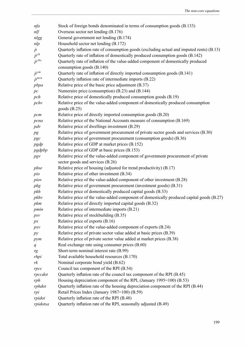
The non-core equations
nfa Stock of foreign bonds denominated in terms of consumption goods (B.133)nlf Overseas sector net lending (B.176)nlgg General government net lending (B.174)nlp Household sector net lending (B.172)p Quarterly inflation rate of consumption goods (excluding actual and imputed rents) (B.13)pch Quarterly rate of inflation of domestically produced consumption goods (B.142)pchv Quarterly rate of inflation of the value-added component of domestically produced
consumption goods (B.140)pcm Quarterly rate of inflation of directly imported consumption goods (B.141)pmin Quarterly inflation rate of intermediate imports (B.22)pbpa Relative price of the basic price adjustment (B.37)pc Numeraire price (consumption) (B.23) and (B.144)pch Relative price of domestically produced consumption goods (B.19)pchv Relative price of the value-added component of domestically produced consumption
goods (B.25)pcm Relative price of directly imported consumption goods (B.20)pcna Relative price of the National Accounts measure of consumption (B.169)pdv Relative price of dwellings investment (B.29)pg Relative price of government procurement of private sector goods and services (B.30)pgc Relative price of government procurement (consumption goods) (B.36)pgdp Relative price of GDP at market prices (B.152)pgdpbp Relative price of GDP at basic prices (B.153)pgv Relative price of the value-added component of government procurement of private
sector goods and services (B.26)phse Relative price of housing (adjusted for trend productivity) (B.17)pio Relative price of other investment (B.34)piov Relative price of the value-added component of other investment (B.28)pkg Relative price of government procurement (investment goods) (B.31)pkh Relative price of domestically produced capital goods (B.33)pkhv Relative price of the value-added component of domestically produced capital goods (B.27)pkm Relative price of directly imported capital goods (B.32)pmin Relative price of intermediate imports (B.21)psv Relative price of stockbuilding (B.35)px Relative price of exports (B.16)pxv Relative price of the value-added component of exports (B.24)py Relative price of private sector value added at basic prices (B.39)pym Relative price of private sector value added at market prices (B.38)q Real exchange rate using consumer prices (B.60)rg Short-term nominal interest rate (B.99)rhpi Total available household resources (B.170)rk Nominal corporate bond yield (B.62)rpcc Council tax component of the RPI (B.54)rpccdot Quarterly inflation rate of the council tax component of the RPI (B.45)rph Housing depreciation component of the RPI, (January 1995=100) (B.53)rphdot Quarterly inflation rate of the housing depreciation component of the RPI (B.44)rpi Retail Prices Index (January 1987=100) (B.59)rpidot Quarterly inflation rate of the RPI (B.48)rpidotsa Quarterly inflation rate of the RPI, seasonally adjusted (B.49)
199
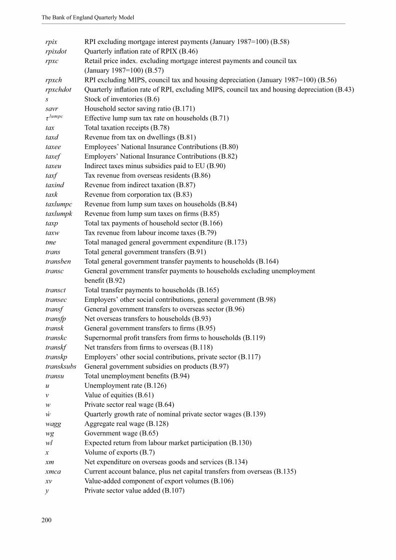
The Bank of England Quarterly Model
rpix RPI excluding mortgage interest payments (January 1987=100) (B.58)rpixdot Quarterly inflation rate of RPIX (B.46)rpxc Retail price index. excluding mortgage interest payments and council tax
(January 1987=100) (B.57)rpxch RPI excluding MIPS, council tax and housing depreciation (January 1987=100) (B.56)rpxchdot Quarterly inflation rate of RPI, excluding MIPS, council tax and housing depreciation (B.43)s Stock of inventories (B.6)savr Household sector saving ratio (B.171)τ lumpc Effective lump sum tax rate on households (B.71)tax Total taxation receipts (B.78)taxd Revenue from tax on dwellings (B.81)taxee Employees’ National Insurance Contributions (B.80)taxef Employers’ National Insurance Contributions (B.82)taxeu Indirect taxes minus subsidies paid to EU (B.90)taxf Tax revenue from overseas residents (B.86)taxind Revenue from indirect taxation (B.87)taxk Revenue from corporation tax (B.83)taxlumpc Revenue from lump sum taxes on households (B.84)taxlumpk Revenue from lump sum taxes on firms (B.85)taxp Total tax payments of household sector (B.166)taxw Tax revenue from labour income taxes (B.79)tme Total managed general government expenditure (B.173)trans Total general government transfers (B.91)transben Total general government transfer payments to households (B.164)transc General government transfer payments to households excluding unemployment
benefit (B.92)transct Total transfer payments to households (B.165)transec Employers’ other social contributions, general government (B.98)transf General government transfers to overseas sector (B.96)transfp Net overseas transfers to households (B.93)transk General government transfers to firms (B.95)transkc Supernormal profit transfers from firms to households (B.119)transkf Net transfers from firms to overseas (B.118)transkp Employers’ other social contributions, private sector (B.117)transksubs General government subsidies on products (B.97)transu Total unemployment benefits (B.94)u Unemployment rate (B.126)v Value of equities (B.61)w Private sector real wage (B.64)w Quarterly growth rate of nominal private sector wages (B.139)wagg Aggregate real wage (B.128)wg Government wage (B.65)wl Expected return from labour market participation (B.130)x Volume of exports (B.7)xm Net expenditure on overseas goods and services (B.134)xmca Current account balance, plus net capital transfers from overseas (B.135)xv Value-added component of export volumes (B.106)y Private sector value added (B.107)
200

The non-core equations
ycap Private sector capacity output (B.15)yd Volume of final demand (B.108)ygap Output growth adjustment term (B.136)ym Private sector value added at market prices (B.109)ystar Potential output (B.100)
Table B.2: Exogenous variables
avhstar Long-run average weekly hours worked in the private sectorcf World tradecpiwedge Wedge between the non-durable consumption deflator and CPI inflation ratesdumq1 Seasonal dummydumq2 Seasonal dummydumq3 Seasonal dummydumq4 Seasonal dummyλ Labour-augmenting technical progressλ Labour-augmenting productivity growthλss Steady-state labour-augmenting productivity growthµcc Weight on council tax in the RPIµcpr Weight on rents in the CPIµmip Weight on MIPS in the RPIµrph Weight on housing depreciation in RPI
Adjustment factor for effect of value of housing on consumptionn Population growthnss Steady-state population growthnhds Population aged 16+, thousandsp f Overseas rate of consumer price inflationpss Domestic inflation targetpgons Relative price of total ONS-measured final general government consumption and
investment expenditurepxf Relative price of world exportspxfdef M6 export prices, using sterling ERI weights, index (1998=100)rf M6 short-term nominal interest raterfprem Premium on overseas interest payments to householdsrgprem Premium on government interest payments to householdsrpixwedge Wedge between the RPI (excluding housing components) and CPI inflation ratessd Statistical discrepancyτ c Effective net indirect tax rate (ratio of basic price adjustment to value added)τ d Effective tax rate on dwellingsτ ee Effective rate of employees’ National Insurance Contributionsτ e f Effective rate of employers’ National Insurance Contributionsτ eu Effective tax rate on EU net indirect taxesτ f Effective tax rate on revenue from overseas residentsτ knd Effective corporation tax rateτ lumpk Effective lump sum tax rate on firmsτw Effective income tax ratetfp Total factor productivity term in production function
201
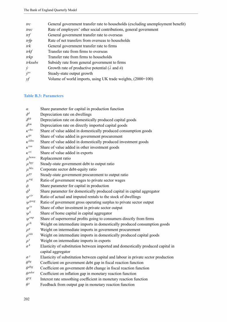
The Bank of England Quarterly Model
trc General government transfer rate to households (excluding unemployment benefit)trec Rate of employers’ other social contributions, general governmenttrf General government transfer rate to overseastrfp Rate of net transfers from overseas to householdstrk General government transfer rate to firmstrkf Transfer rate from firms to overseastrkp Transfer rate from firms to householdstrksubs Subsidy rate from general government to firmsy Growth rate of productive potential (λ and n)yss Steady-state output growthyf Volume of world imports, using UK trade weights, (2000=100)
Table B.3: Parameters
α Share parameter for capital in production functionδd Depreciation rate on dwellingsδkh Depreciation rate on domestically produced capital goodsδkm Depreciation rate on directly imported capital goodsκchv Share of value added in domestically produced consumption goodsκgv Share of value added in government procurementκ ikhv Share of value added in domestically produced investment goodsκ iov Share of value added in other investment goodsκ xv Share of value added in exportsµbenw Replacement ratioµbgy Steady-state government debt to output ratioµbkv Corporate sector debt-equity ratioµgy Steady-state government procurement to output ratioµwg Ratio of government wages to private sector wagesφ Share parameter for capital in productionφk Share parameter for domestically produced capital in capital aggregatorψcir Ratio of actual and imputed rentals to the stock of dwellingsψgosg Ratio of government gross operating surplus to private sector outputψ io Share of other investment in private sector outputψk Share of home capital in capital aggregatorψ snp Share of supernormal profits going to consumers directly from firmsρch Weight on intermediate imports in domestically produced consumption goodsρg Weight on intermediate imports in government procurementρikh Weight on intermediate imports in domestically produced capital goodsρx Weight on intermediate imports in exportsσ k Elasticity of substitution between imported and domestically produced capital in
capital aggregatorσ y Elasticity of substitution between capital and labour in private sector productionθbg Coefficient on government debt gap in fiscal reaction functionθdbg Coefficient on government debt change in fiscal reaction functionθ pdot Coefficient on inflation gap in monetary reaction functionθ rg Interest rate smoothing coefficient in monetary reaction functionθ y Feedback from output gap in monetary reaction function
202

The non-core equations
B.2 Non-core equations
This section sets out the non-core equations under general headings, highlighting and collecting togetherequations that determine similar variables (such as demand components, prices and inflation and labourmarket variables), rather than following the order of the core model equations in Appendix A.Econometric results for the estimated equations are reported and discussed in Section 6.4.2.
A number of technical points are worth noting first:
• most of the equations are written in detrended model units (as are all of the core model equationslisted in Appendix A). Box 12 on page 88 explains that this means that terms involving lags willgenerally be scaled according to some combination of productivity growth, population growth andinflation. We do not comment on these growth terms unless they are particularly important for theinterpretation of the equation;
• we therefore need to add ‘growth adjustment’ terms so that our specifications imply partialadjustment in actual (ie not model) units. These growth adjustment terms are ygap, ngap and λgap
and are defined in equations (B.136), (B.137) and (B.138). These terms are zero over our historicalsample, and hence not included in the estimation results reported in Chapter 6. But they will benon-zero in the event of productivity or population shocks;
• we also add a number of recursive ‘post-transformation’ equations, which convert solutions inmodel units into units that are more directly comparable to National Accounts measures. Many ofthese are simple reversals of transformations listed in Appendix C. Others, including those thatrequire some explanation, are listed in Section B2.8;
• the price of non-durable consumption bundle (PC) is the numeraire. This implies that the relativeprice of non-durable consumption, pc, is set equal to 1 in every period – see equation (B.23) below.As in the core model listing, we often implicitly impose this condition in the equations (ie weeliminate terms in pc) but it appears explicitly when its inclusion may help to interpret the equation;
• We use the symbol to indicate a change operator – so that xt = xt − xt−1, andxt−1 = xt−1 − xt−2. Solutions from the core model are denoted by the core superscript and
non-core equation residuals are denoted by the res superscript (see equation (B.4) for a simpleexample) and steady-state values are denoted by the ss superscript; and
• accounting relationships are often identical to core model equations, with the exception of anadditional residual term. We describe such equations as identical to the core version, despite thepresence of the residual. The residuals in the non-core versions of the equations also act as a crosscheck on the data transformations process used to generate the data set.
B2.1 Demand components
The aggregate (non-durable) consumption equation (B.1) contains an error correction to non-durableconsumption. An extra argument in assets is included to ensure convergence in net foreign assets.Proxy variables for effects missing from the core include changes in the value of the housing stock, as aproxy for housing collateral effects; changes in household income, as a proxy for the existence ofrule-of-thumb individuals; changes in the employment rate, as a proxy for confidence and uncertaintyeffects; and changes in nominal interest rates, as a proxy for credit and cash-flow effects.
The variable t is an exogenous variable that allows us to change the size of the effect on consumptionof changes in the value of housing. The box on pages 12-13 of the November 2004 Inflation Reportexplained how, in the recent past, the association between house price inflation and consumption has
203
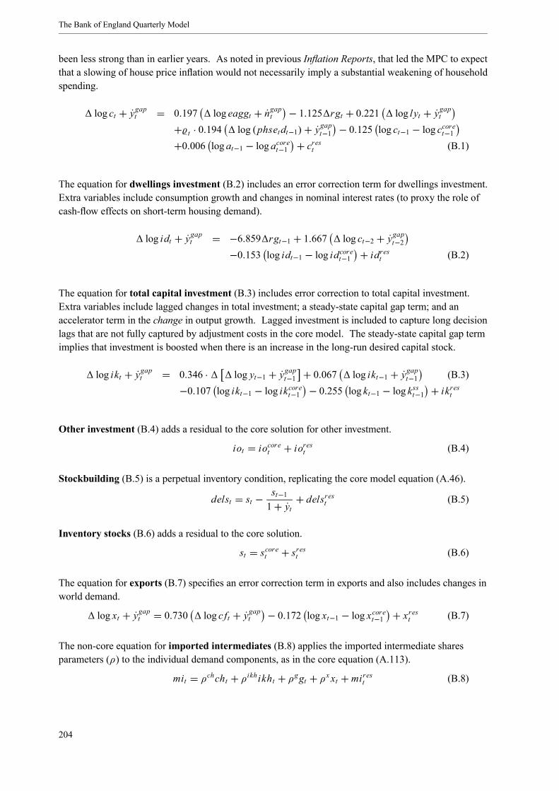
The Bank of England Quarterly Model
been less strong than in earlier years. As noted in previous Inflation Reports, that led the MPC to expectthat a slowing of house price inflation would not necessarily imply a substantial weakening of householdspending.
log ct + ygapt = 0.197 log eaggt + ngapt − 1.125 rgt + 0.221 log lyt + ygapt
+ t · 0.194 log (phsetdt−1)+ ygapt−1 − 0.125 log ct−1 − log ccoret−1+0.006 log at−1 − log acoret−1 + crest (B.1)
The equation for dwellings investment (B.2) includes an error correction term for dwellings investment.Extra variables include consumption growth and changes in nominal interest rates (to proxy the role ofcash-flow effects on short-term housing demand).
log idt + ygapt = −6.859 rgt−1 + 1.667 log ct−2 + ygapt−2−0.153 log idt−1 − log idcoret−1 + idrest (B.2)
The equation for total capital investment (B.3) includes error correction to total capital investment.Extra variables include lagged changes in total investment; a steady-state capital gap term; and anaccelerator term in the change in output growth. Lagged investment is included to capture long decisionlags that are not fully captured by adjustment costs in the core model. The steady-state capital gap termimplies that investment is boosted when there is an increase in the long-run desired capital stock.
log ikt + ygapt = 0.346 · log yt−1 + ygapt−1 + 0.067 log ikt−1 + ygapt−1 (B.3)−0.107 log ikt−1 − log ikcoret−1 − 0.255 log kt−1 − log ksst−1 + ikrest
Other investment (B.4) adds a residual to the core solution for other investment.
iot = iocoret + iorest (B.4)
Stockbuilding (B.5) is a perpetual inventory condition, replicating the core model equation (A.46).
delst = st − st−11+ yt + dels
rest (B.5)
Inventory stocks (B.6) adds a residual to the core solution.
st = scoret + srest (B.6)
The equation for exports (B.7) specifies an error correction term in exports and also includes changes inworld demand.
log xt + ygapt = 0.730 log c ft + ygapt − 0.172 log xt−1 − log xcoret−1 + xrest (B.7)
The non-core equation for imported intermediates (B.8) applies the imported intermediate sharesparameters (ρ) to the individual demand components, as in the core equation (A.113).
mit = ρchcht + ρikhikht + ρggt + ρx xt + mirest (B.8)
204
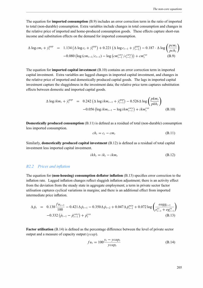
The non-core equations
The equation for imported consumption (B.9) includes an error correction term in the ratio of importedto total (non-durable) consumption. Extra variables include changes in total consumption and changes inthe relative price of imported and home-produced consumption goods. These effects capture short-runincome and substitution effects on the demand for imported consumption.
log cmt + ygapt = 1.134 log ct + ygapt + 0.221 log ct−1 + ygapt−1 − 0.187 · logpcmtpcht
−0.080 log (cmt−1/ct−1)− log cmcoret−1 /ccoret−1 + cmrest (B.9)
The equation for imported capital investment (B.10) contains an error correction term in importedcapital investment. Extra variables are lagged changes in imported capital investment, and changes inthe relative price of imported and domestically produced capital goods. The lags in imported capitalinvestment capture the sluggishness in the investment data; the relative price term captures substitutioneffects between domestic and imported capital goods.
log ikmt + ygapt = 0.242 log ikmt−1 + ygapt−1 − 0.526 logpkmtpkht
−0.056 log ikmt−1 − log ikmcoret−1 + ikmrest (B.10)
Domestically produced consumption (B.11) is defined as a residual of total (non-durable) consumptionless imported consumption.
cht = ct − cmt (B.11)
Similarly, domestically produced capital investment (B.12) is defined as a residual of total capitalinvestment less imported capital investment.
ikht = ikt − ikmt (B.12)
B2.2 Prices and inflation
The equation for (non-housing) consumption deflator inflation (B.13) specifies error correction to theinflation rate. Lagged inflation changes reflect sluggish inflation adjustment; there is an activity effectfrom the deviation from the steady state in aggregate employment; a term in private sector factorutilisation captures cyclical variations in margins; and there is an additional effect from importedintermediate price inflation.
pt = 0.138f ut−1100
− 0.421 pt−1 − 0.350 pt−2 + 0.047 pmint−1 + 0.072 logeaggt−1
esst−1 + egsst−1−0.332 pt−1 − pcoret−1 + prest (B.13)
Factor utilisation (B.14) is defined as the percentage difference between the level of private sectoroutput and a measure of capacity output (ycap).
f ut = 100 yt − ycaptycapt(B.14)
205
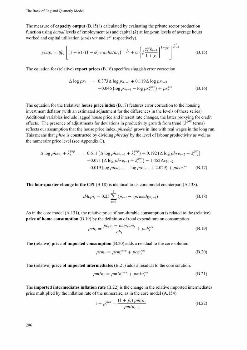
The Bank of England Quarterly Model
The measure of capacity output (B.15) is calculated by evaluating the private sector productionfunction using actual levels of employment (e) and capital (k) at long-run levels of average hoursworked and capital utilisation (avhstar and zss respectively).
ycapt = tfpt (1− α) {(1− φ) etavhstart}1−1σ y + α φ
zsst kt−11+ yt
1− 1σ y
σ yσ y−1
(B.15)
The equation for (relative) export prices (B.16) specifies sluggish error correction.
log pxt = 0.373 log pxt−1 + 0.119 log pxt−3−0.046 log pxt−1 − log pxcoret−1 + pxrest (B.16)
The equation for the (relative) house price index (B.17) features error correction to the housinginvestment deflator (with an estimated adjustment for the differences in the levels of these series).Additional variables include lagged house price and interest rate changes, the latter proxying for crediteffects. The presence of adjustments for deviations in productivity growth from trend (λgap terms)reflects our assumption that the house price index, phsedef, grows in line with real wages in the long run.This means that phse is constructed by dividing phsedef by the level of labour productivity as well asthe numeraire price level (see Appendix C).
log phset + λgapt = 0.611 log phset−1 + λgapt−1 + 0.192 log phset−2 + λgapt−2+0.071 log phset−3 + λgapt−3 − 1.452 rgt−2−0.019 (log phset−1 − log pdvt−1 + 2.029)+ phserest (B.17)
The four-quarter change in the CPI (B.18) is identical to its core model counterpart (A.138).
d4cpit = 0.253
i=0( pt−i − cpiwedget−i ) (B.18)
As in the core model (A.131), the relative price of non-durable consumption is related to the (relative)price of home consumption (B.19) by the definition of total expenditure on consumption.
pcht = pctct − pcmtcmtcht
+ pchrest (B.19)
The (relative) price of imported consumption (B.20) adds a residual to the core solution.
pcmt = pcmcoret + pcmrest (B.20)
The (relative) price of imported intermediates (B.21) adds a residual to the core solution.
pmint = pmincoret + pminrest (B.21)
The imported intermediates inflation rate (B.22) is the change in the relative imported intermediatesprice multiplied by the inflation rate of the numeraire, as in the core model (A.154).
1+ pmint = (1+ pt) pmintpmint−1
(B.22)
206
The non-core equations
As in the core model, the non-durable consumption price is the numeraire, so by definition the relativeprice of non-durable consumption (B.23) is equal to 1.
pct = 1 (B.23)
The (relative)market price of exports (B.24) is given by the weighted average of the prices ofdomestically produced consumption, imported intermediates and indirect taxes. The core modelequation (A.136) is identical.
pxt = κ xv pxvt + ρx pmint + 1− ρx − κ xv pbpat (B.24)
Equations for themarket price of home consumption (B.25), themarket price of governmentprocurement (B.26), themarket price of home capital (B.27) and themarket price of otherinvestment (B.28) are constructed analogously. The core model equivalents are equations(A.132),(A.135), (A.133) and (A.137).
pcht = κchv pchvt + ρch pmint + 1− κchv − ρch pbpat (B.25)
pgt = κgv pgvt + ρg pmint + 1− κgv − ρg pbpat (B.26)
pkht = κ ikhv pkhvt + ρikh pmint + 1− κ ikhv − ρikh pbpat (B.27)
piot = κ iov piovt + 1− κ iov pbpat (B.28)
The (relative) price of dwellings (B.29) adds a residual to the core solution. The logarithmic equationform implies that residuals can be treated as percentage differences between the core and non-coresolutions.
log pdvt = log pdvcoret + pdvrest (B.29)
The equations for the (relative) prices of government procurement (B.30), government procurementof investment goods (B.31), imported capital (B.32), home capital (B.33), other investment (B.34)and inventory stocks (B.35) add residuals to the core solutions. This means that variations in therelative prices of the components of government procurement are modelled by residual adjustment.
pgt = pgcoret + pgrest (B.30)
pkgt = pgcoret + pkgrest (B.31)
pkmt = pkmcoret + pkmrest (B.32)
pkht = pkhcoret + pkhrest (B.33)
piot = piocoret + piorest (B.34)
psvt = psvcoret + psvrest (B.35)
207
The Bank of England Quarterly Model
The (relative) price of government procurement of consumption goods (B.36) is derived from thedifference between the values of total and investment procurement.
pgct = (pgt · gt − pkgt · igt)gct+ pgcrest (B.36)
The (relative) price of the basic price adjustment (B.37) moves to ensure that revenue from the basicprice adjustment (product taxation) is an exogenous fraction τ c of the value of private sector output.This corresponds to a long-run version of the core model equation (A.141).
pbpat = τ ctpyt yt
ymt − yt + pbparest (B.37)
Themarket price of private sector output (B.38) is given by the value of marketed output measured atmarket prices, adjusted for imported intermediates and divided by the volume of private sector output atmarket prices, ym. This replicates the core model (A.139) apart from the addition of a term for thestatistical discrepancy between the average and expenditure measures of GDP.
pymt ymt = pchtcht + pdvt idt + pkht ikht + piot iot + psvt delst + pgt gt+pxt xt − pmintmit + sdexpt (B.38)
The basic price of private sector output (B.39) is defined by subtracting the value of the basic priceadjustment from the market value of private production, then dividing by private sector output. This isidentical to the core model equation (A.140).
pyt = pymt ymt − pbpat (ymt − yt)yt
+ pyrest (B.39)
The inflation rate of Consumer Prices Index (CPI) excluding rents (B.40) is the inflation rate ofnon-durable consumption prices adjusted for the average wedge between that and CPI inflation, plus aresidual, which mainly captures the seasonal component of cpixr .
cpixrdott = pt − cpiwedget + cpixrdotrest (B.40)
The inflation rate of the rents component of the CPI (B.41) is given by the inflation rate ofnon-durable consumption prices adjusted for the average wedge between that and CPI inflation, plus aresidual. The residual again captures the seasonal components of the index, but also any deviation of theinflation rate of rents from the other components in the CPI basket.
cprdott = pt − cpiwedget + cprdotrest (B.41)
CPI inflation (B.42) is given by the weighted average of the rents and non-rents components. Theresidual mainly captures differences in the rounding of sub-indices used to construct the overall index.
cpidott = µcpr cprdott + 1− µcpr cpi xrdott + cpidotrest (B.42)
Inflation of the Retail Prices Index (RPI) excluding various housing factors (council tax, housingdepreciation and mortgage interest payments) (B.43) adjusts the CPI inflation rate for the wedgebetween the two measures. This wedge is mainly driven by the ‘formula effect’ arising from the use ofarithmetic averaging of price quotes to construct the RPI, compared with geometric averaging used toconstruct the CPI.
rpxchdott = cpidott + rpi xwedget + rpxchdotrest (B.43)
208
The non-core equations
The housing depreciation component of the RPI (B.44) is an exponentially smoothed house priceindex. This implies that housing depreciation inflation is a weighted average of current and past houseprice inflation and past housing depreciation inflation. The residual captures the fact that the model’shouse price index, phsedef, is not the house price index that underlies rph.
rphdott = 0.5phsetphset−1
(1+ pt) 1+ λt − 1 + 0.25 phset−1phset−2
(1+ pt−1) 1+ λt−1 − 1+0.25 · rphdott−1 + rphdotrest (B.44)
The council tax component of RPI inflation (B.45) is the rate of growth of nominal council tax revenue(taxd) adjusted for the growth in the housing stock, multiplied by a seasonal dummy, dumq2. (1)
rpccdott = dumq2t 1+ λt (1+ nt) taxdt (1+ pt)taxdt−1
− dtdt−1
+ rpccdotrest (B.45)
RPIX inflation (which measures RPI inflation excluding mortgage interest payments) (B.46) is theweighted averages of the sub-indices rpccdot , rphdot and rpxchdot . The residual captures the effectof the different rounding conventions used in the sub-indices.
rpi xdott = µcc
1− µmip rpccdott +µrph
1− µmip rphdott
+ 1− µrph + µcc1− µmip rpxchdott + rpi xdotrest (B.46)
Inflation of mortgage interest payments (B.47) is proxied using the rate of inflation of interestpayments on the nominal value of the housing stock, evaluated using the house price index phse.
mipsdott = rgtrgt−1
− 1 + phset (1+ pt) 1+ λtphset−1
− 1
+ dt 1+ λt (1+ nt)dt−1
− 1 +mipsdotrest (B.47)
RPI inflation (B.48) is the weighted average of the sub-indices mipsdot and rpixdot . Again, theresidual captures rounding effects.
rpidott = µmipmipsdott + 1− µmip rpi xdott + rpidotrest (B.48)
Seasonally adjusted RPI inflation (B.49) adjusts RPI inflation for seasonal effects using seasonaldummy variables.
rpidotsat = rpidott + 0.0017dumq1t − 0.005dumq2t+0.0035dumq3t − 0.0002dumq4t + rpidotsarest (B.49)
(1) This dummy takes the value 1 in second quarter of each year and zero otherwise. It is used here because changes incouncil tax rates are ordinarily implemented in the second quarter of each year.
209
The Bank of England Quarterly Model
The levels of the non-rent component (B.50) and rent component (B.51) of the CPI are given bycumulating the inflation rates of these series.
cpixrt = cpixrt−1 (1+ cpi xrdott) (B.50)
cprt = cprt−1 (1+ cprdott) (B.51)
The level of the CPI (B.52) is a chain-weighted index of cpixr and cpr , where the residual arises froman approximation error owing to chaining the indices quarterly rather than monthly.
cpit =4
i=1dumqitcpit−i× (1− µcpr ) cpixrt
4i=1 dumqitcpi xrt−i
+ µcpr cprt4i=1 dumqitcprt−i
× 1+ cpirest (B.52)
The levels of the housing depreciation component (B.53), council tax component (B.54),mortgageinterest payments component (B.55) of RPI and RPI excluding these components (B.56) are givenby cumulating the inflation rates of these variables.
rpht = rpht−1 (1+ rphdott) (B.53)
rpcct = rpcct−1 (1+ rpccdott) (B.54)
mipst = mipst−1 (1+mipsdott) (B.55)
rpxcht = rpxcht−1 (1+ rpxchdott) (B.56)
The level of the RPIX excluding council tax (B.57) is a chain-weighted index of rph and rpxch, wherethe residual arises from an approximation error owing to chaining the indices quarterly rather thanmonthly.
rpxct = (dumq1tr pxct−4 + dumq2tr pxct−1 + dumq3tr pxct−2 + dumq4tr pxct−3)
×⎡⎣ µrph
1−µmip−µccrpht
dumq1t r pht−4+dumq2t r pht−1+dumq3t r pht−2+dumq4t r pht−3+ 1− µrph
1−µmip−µccrpxcht
dumq1t r pxcht−4+dumq2t r pxcht−1+dumq3t r pxcht−2+dumq4t r pxcht−3
⎤⎦× 1+ rpxcrest (B.57)
The level of the RPIX excluding mortgage interest payments (B.58) is a chain-weighted index ofrpcc and rpxc, where the residual arises from an approximation error owing to chaining the indicesquarterly rather than monthly.
rpi xt = (dumq1tr pi xt−4 + dumq2tr pi xt−1 + dumq3tr pi xt−2 + dumq4tr pi xt−3)
×µcc
1−µmiprpcct
dumq1t r pcct−4+dumq2t r pcct−1+dumq3t r pcct−2+dumq4t r pcct−3+ 1− µcc
1−µmiprpxct
dumq1t r pxct−4+dumq2t r pxct−1+dumq3t r pxct−2+dumq4t r pxct−3× 1+ rpixrest (B.58)
210
The non-core equations
The level of the RPI (B.59) is a chain-weighted index of rpi x and mips, where the residual arises froman approximation error owing to chaining the indices quarterly rather than monthly. We can use asimilar method to construct other measures, such as the RPIY.
rpit = (dumq1tr pit−4 + dumq2tr pit−1 + dumq3tr pit−2 + dumq4tr pit−3)× µmip mipst
dumq1tmipst−4+dumq2tmipst−1+dumq3tmipst−2+dumq4tmipst−3+ 1− µmip rpi xt
dumq1t r pi xt−4+dumq2t r pixt−1+dumq3t r pi xt−2+dumq4t r pi xt−3× 1+ rpirest (B.59)
B2.3 Asset prices
The real exchange rate (B.60), the value of equities (B.61) and the interest rate on corporate debt(B.62) all take the core model value plus a residual.
qt = qcoret + qrest (B.60)
vt = vcoret + vrest (B.61)
rkt = rkcoret + rkrest (B.62)
Corporate debt issuance (B.63) is a given ratio (µbk) of the equity value plus a residual. This equationcorresponds to a long-run version of the core model equation (A.47).
bkt = µbkvvt + bkrest (B.63)
B2.4 Labour market
The equation for private sector real wages (B.64) includes an error correction term in core privatesector real wages. Extra variables include lagged real wage growth and changes in RPI inflation, whichare likely to influence wage setting; terms in RPI and the change in the consumption deflator, reflectingthe wedge between the two measures (in effect the equation is estimated on nominal wages deflated byRPI); and the gap between the unemployment rate and steady-state unemployment, to capture cyclicalinfluences on wage setting.
logwt + pt − rpidotsat + λgapt = 0.508 logwt−1 + λgapt−1 + pt−1 − rpidotsat−1−0.488 rpidotsat − 0.599 rpidotsat−1−0.519 rpidotsat−2 − 0.120 ut − usst−0.420 logwt−1 − logwcoret−1 +wrest (B.64)
The equation for public sector real wages (B.65) includes an error correction term in private sector realwages, adjusted for the wedge between public and private sector wages. An additional term in laggedpublic sector real wage growth captures sluggishness in real wage adjustment.
logwgt + λgapt = 0.348 logwt−1 + λgapt−1−0.166 log(wgt−1)− log µwgwt−1 +wgrest (B.65)
211
The Bank of England Quarterly Model
The equation for private sector employment (B.66) specifies an error correction to private sectoremployment. Extra variables include lagged changes in private sector employment and changes inprivate sector output. These terms proxy sluggish employment adjustment and labour demand effectsrespectively. A lagged term in factor utilisation is also included, as increases in factor utilisation tend toraise subsequent employment growth.
log et + ngapt = 0.649 log et−1 + ngapt−1 + 0.094 log yt + ygapt
+0.053 f ut−1100
− 0.031 log et−1 − log ecoret−1 + erest (B.66)
The equation for average hours (B.67) includes an error correction term for average hours. Additionaldynamic terms include lagged growth in average hours and private sector output – reflecting sluggishadjustment and labour demand effects respectively.
log avht = 0.560 log avht−1 + 0.037 log yt + ygapt + 0.055 log yt−1 + ygapt−1−0.048 log avht−1 − log avhcoret−1 + avhrest (B.67)
The equation for participation (B.68) includes an error correction term in participation. Extra variablesinclude lagged participation growth (reflecting sluggish labour market adjustment) and changes inaverage real wages (as a proxy for the return to entry into the labour market).
log lt + ngapt = 0.499 log lt−1 + ngapt−1 + 0.249 log lt−2 + ngapt−2+0.044 log
wt−2et−2 +wgt−2egt−2eaggt−2
+ λgapt−2−0.099 log lt−1 − log lcoret−1 + lrest (B.68)
Private sector employment in hours (B.69) is a logarithmic version of the core equivalent (A.71).
log eht = log et + log avht + ehrest (B.69)
B2.5 Government
The government budget constraint (B.70), fiscal reaction function (B.71) and government debttarget (B.72) are the same as the core equivalents (A.79), (A.80), (A.81).
pgtbgt = 1+ rgt−11+ pt
pgt−1bgt−11+ yt + pct−1mont−1
(1+ pt) (1+ yt) + pgt gt + (1+ ecostgt)wgtegt+gosgexpt + transt − taxt − pctmont + bgrest (B.70)
τlumpct = τ lumpct−1 + θbg bgt − bgtart
pyt yt+ θdbg bgt
pyt yt− bgt−1pyt−1yt−1
+ taulumpcrest (B.71)
bgtart = µbgy pyt ytpgt+ bgtarrest (B.72)
212
The non-core equations
The non-core equations for government wage spending (B.73), government procurement (B.74) andgovernment investment procurement (B.75) run off the core model solutions (A.84), (A.82) and(A.86).
(1+ ecostgt)wgtegt = (1+ ecostgt)wgcoret egcoret + egrest (B.73)
pgt gt = pgcoret gcoret + grest (B.74)
igt = igcoret + igrest (B.75)
Government consumption procurement (B.76) subtracts investment procurement from totalprocurement.
gct = gt − igt + gcrest (B.76)
The government’s gross operating surplus (B.77) adds a residual to the core model solution (A.89).
gosgexpt = gosgexpcoret + gosgexprest (B.77)
Total tax revenue (B.78) is the same as the core equivalent (A.90).
taxt = taxwt + taxeet + taxdt + taxef t + taxkt + taxlumpct + taxlumpkt + taxf t+taxindt + gosgexpt + taxrest (B.78)
Income tax revenue (B.79), employees’ National Insurance Contributions (B.80), dwellings taxrevenue (B.81), employers’ National Insurance Contributions (B.82), corporation tax revenue(B.83), lump sum tax revenue from consumers (B.84), lump sum tax revenue from firms (B.85), taxrevenue from overseas (B.86), indirect tax revenue (B.87) the total wage tax rate for private sectorfirms (B.88), total wage tax rate for government (B.89), net indirect taxes paid to the EuropeanUnion (B.90), total transfer payments from government (B.91), transfers to consumers (B.92),transfers from overseas (B.93), total unemployment benefits (B.94), transfers to firms (B.95),transfers to overseas (B.96), transfers subsidies to firms on products (B.97) and socialcontributions paid to government employees (B.98) are all defined in the same way as the core model.The corresponding core model equations are (A.20) and (A.91) to (A.108).
taxwt = τwt (wt et + wgtegt)+ taxwrest (B.79)
taxeet = τ eet (wt et +wgtegt)+ taxeerest (B.80)
taxdt = τ dt pdvt dt + taxdrest (B.81)
taxef t = τ e ft (wt et +wgtegt)+ taxef rest (B.82)
taxkt = τ kndt pyt yt + taxkrest (B.83)
taxlumpct = τ lumpct yt pyt + taxlumpcrest (B.84)
213
The Bank of England Quarterly Model
taxlumpkt = τ lumpkt yt pyt + taxlumpkrest (B.85)
taxf t = τ ft yt pyt + taxf rest (B.86)
taxindt = pbpat (ymt − yt)+ transksubst − taxeut + taxindrest (B.87)
ecostt = τ e ft + trkpt + ecostrest (B.88)
ecostgt = τ e ft + trect (B.89)
taxeut = τ eut pyt yt + taxeurest (B.90)
transt = transct + transut + transkt + transf t + transksubst + rgpremt + transrest (B.91)
transct = trct yt pyt + transcrest (B.92)
transfpt = trfpt yt pyt + transfprest (B.93)
transut = bentutlt + transurest (B.94)
transkt = trkt yt pyt + transkrest (B.95)
transf t = trf t yt pyt + transf rest (B.96)
transksubst = trksubst yt pyt + transksubsrest (B.97)
transect = trectwgtegt + transecrest (B.98)
B2.6 Monetary authority
The monetary reaction function (B.99) takes the same form and coefficients as the core modelequation (A.110). The only difference is that the non-core reaction function depends on the core modelsolution for the nominal interest rate (rather than the steady-state nominal interest rate).
rgt = 1− θ rg rgcoret + θ pdot d4cpit − psst + θ y log yt + gltystart
+ θ rgrgt−1 + rgrest (B.99)
The policy reaction function depends on potential output (B.100), which is measured in a similar wayto the core model equation (A.111).
ystart = tfpt (1− α) (1− φ) 1− usst lsst avhstart1− 1
σ y + α φzsst kt−11+ yt
1− 1σ y
σ yσ y−1
(B.100)
214
The non-core equations
As in the core model (A.112), the level of demand entering the policy rule is given by private sectoroutput (y) plus the government demand for resources (B.101) expressed in terms of private sectoroutput.
glt = tfpt (1− α) {(1− φ) eaggtavhstart}1−1σ y + α φ
zsst kt−11+ yt
1− 1σ y
σ yσ y−1
−tfpt (1− α) {(1− φ) etavhstart}1−1σ y + α φ
zsst kt−11+ yt
1− 1σ y
σ yσ y−1
(B.101)
B2.7 Accounting and reporting
The (basic price) value-added components of home consumption (B.102), home capital investment(B.103), other investment (B.104), government procurement (B.105) and exports (B.106) areidentical to the core model equations (A.142) to (A.146).
chvt = κchvcht (B.102)
ikhvt = κ ikhv ikht (B.103)
iovt = κ iov iot (B.104)
gvt = κgvgt (B.105)
xvt = κ xvxt (B.106)
The level of demand for private sector output at basic prices (B.107) is defined as the sum of marketprice domestic demand components net of imports and the basic price adjustment. The statisticaldiscrepancy (sd) is also included in this definition of demand.
yt = ct + idt + ikt + iot + delst + gt + xt − cmt − ikmt −mit+sdt − bpat + yrest (B.107)
The level of demand for private sector output excluding stockbuilding (B.108) is identical to the coremodel counterpart (A.45).
ydt = chvt + idt + ikhvt + iovt + gvt + xvt (B.108)
The level of demand for private sector output at market prices (B.109) is given by the demand forprivate sector output at basic prices, plus the basic price adjustment.
ymt = yt + bpat + ymrest (B.109)
215
The Bank of England Quarterly Model
The basic price adjustment (B.110) is defined as the sum of the contributions from each expenditurecategory. It is given by the difference between the market price volume and the sum of domesticallyproduced value added (proportion κ) and imported intermediate components (proportion ρ).
bpat = 1− κchv − ρch cht + 1− κ ikhv − ρikh ikht + 1− κ iov iot+ 1− κgv − ρg gt + 1− κ xv − ρx xt + bparest (B.110)
Expenditure on other investment (B.111) is given by the volume of other investment multiplied by therelative price.
ioexpt = piot iot + ioexprest (B.111)
The volume of imputed and other rents (B.112) is equal to the core solution plus a residual.
cirt = circoret + cirrest (B.112)
Expenditure on imputed and other rents (B.113) is a proportion of the value of the dwellings stock.
cirexpt = ψcir pdvt dt + cirexprest (B.113)
The household budget constraint (B.114) replicates the core model equation (A.4).
b ft pctqt
+ pgtbgt + vt + bkt = pct−1mont−1(1+ yt) (1+ pt) − pct · mont +
1+ r ft−11+ p ft
b ft−11+ yt
pctqt
+1+ rgt−11+ pt
pgt−1bgt−11+ yt + vt + dvt + 1+ rkt−11+ pt
bkt−11+ yt
+wlt lt − pctct + transct + transkct + transkpt + transfpt+rfpremt + rgpremt − taxlumpct + transect−pdvt dt − 1− δdt dt−1
1+ yt − τ dt pdvt dt + b f rest (B.114)
The level of real money balances (B.115) relative to consumption is equal to the ratio in the core model(adjusted for a residual).
mont = moncoret
ccoretct +monrest (B.115)
The definition of dividends (B.116) is identical to the core model expression (A.25).
dvt = pchvt chvt + pkhvt ikhvt + pdvt idt + piovt iovt + psvt delst + gvt · pgvt + pxvt xvt− (1+ ecostt)wt et − pkht ikht − psvt delst − transkct − pkmtikmt − piot iot− rkt−1bkt−1(1+ yt) (1+ pt) + bkt −
bkt−1(1+ yt) (1+ pt)
−taxkt − taxlumpkt − transkf t + transkt (B.116)
Employers’ private social contributions (B.117) to consumers are given by the application of atransfer weight (trkp) to the pre-tax private sector wage bill, as in the core model equation (A.49).
transkpt = trkptwt et + transkprest (B.117)
216
The non-core equations
Transfers from firms to overseas (B.118) is defined identically to the core model equation (A.50).
transkf t = trkf t pyt yt + transkf rest (B.118)
Transfers from firms to consumers (B.119) are given by a proportion of the value of private sectoroutput as in the core model (A.48).
transkct = ψ snp pyt yt (B.119)
Total asset holdings (B.120) include the values of equities corporate bonds, government bonds, realmoney balances and net foreign assets, as in the core model (A.158).
at = vt + bkt + pgtbgt + pctmont + nfat (B.120)
The cumulation equation for the dwellings stock (B.121) is identical to the core model equation (A.12).
dt = 1− δdt dt−11+ yt + idt + drest (B.121)
The cumulation equations for the home capital stock (B.122) and the imported capital stock (B.123)are similar to the core model, but the effective depreciation rates are not adjusted for capital utilisation.
kht = 1− δkht kht−11+ yt + ikht + khrest (B.122)
kmt = 1− δkmt kmt−11+ yt + ikmt + kmrest (B.123)
The CES function defining the capital index (B.124) as a function of home and imported capitalreplicates the core model equation (A.27).
kt = ψk φkkht1− 1
σk + 1− ψk 1− φk kmt 1−1σk
σ kσk−1
(B.124)
Total labour income (B.125) is the effective wage rate from participating in the labour marketmultiplied by the participation rate, plus transfers to consumers.
lyt = wlt lt + transct (B.125)
The unemployment rate (B.126) is defined as in the core model (A.66).
ut = lt − ent − egtlt(B.126)
Aggregate employment (B.127) is the sum of private and public sector employment.
eaggt = ent + egt (B.127)
The aggregate wage rate (B.128) is a weighted average of public and private sector wage rates.
waggt = egtwgt + (eaggt − egt)wteaggt(B.128)
217
The Bank of England Quarterly Model
Private sector employment in heads (B.129) is set equal to the employment index (e).
ent = et (B.129)
The expected wage from participation (B.130) is identical to the core model equation (A.62).
wlt = 1− ut − µegt 1− τwt − τ eet wt + utbent + µegt 1− τwt − τ eet wgt (B.130)
Unemployment benefits (B.131) are given by an exogenous ratio of the private sector pre-tax wage, asin the core model (A.70).
bent = µbenwwt (B.131)
The share of public sector employment in participation (B.132) is defined analogously to the coremodel equation (A.68).
µegt = egtlt (B.132)
Net foreign assets (B.133), the trade balance (B.134) and the current account are identical to the coremodel equations (A.150), (A.151) and (A.152).
nfat =bft pctqt
+ nfarest (B.133)
xmt = pxt xt − pcmtcmt − pkmtikmt − pmintmit (B.134)
xmcat = pxt xt − pcmtcmt − pkmtikmt − pmintmit + taxf t − transf t − transkf t+transfpt − taxeut + rfpremt +
r ft−1nfat−1(1+ pt) (1+ yt) + xmca
rest (B.135)
As noted in the introductory remarks to this section, the non-core model equations make use of technicalterms ygap, λgap and ngap to ensure that the partial adjustment mechanisms operate in actual units ratherthan model units. The expressions for these growth adjustments are given by equations (B.136),(B.137) and (B.138). These growth adjustments are simply equal to the deviation between the observedgrowth rate and the steady-state growth rate, denoted by the superscript ss.
ygapt = log (1+ yt)− log 1+ ysst (B.136)
λgapt = log 1+ λt − log 1+ λsst (B.137)
ngapt = log (1+ nt)− log 1+ nsst (B.138)
Nominal private sector wage inflation (B.139) is calculated as the change in the real wage multipliedby the numeraire inflation rate and the change in labour productivity, as in the core model (A.157).
1+ wt = (1+ pt) 1+ λt wtwt−1
(B.139)
218
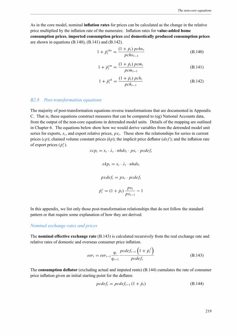
The non-core equations
As in the core model, nominal inflation rates for prices can be calculated as the change in the relativeprice multiplied by the inflation rate of the numeraire. Inflation rates for value-added homeconsumption prices, imported consumption prices and domestically produced consumption pricesare shown in equations (B.140), (B.141) and (B.142).
1+ pchvt = (1+ pt) pchvtpchvt−1
(B.140)
1+ pcmt = (1+ pt) pcmtpcmt−1
(B.141)
1+ pcht =(1+ pt) pchtpcht−1
(B.142)
B2.8 Post-transformation equations
The majority of post-transformation equations reverse transformations that are documented in AppendixC. That is, these equations construct measures that can be compared to (eg) National Accounts data,from the output of the non-core equations in detrended model units. Details of the mapping are outlinedin Chapter 6. The equations below show how we would derive variables from the detrended model unitseries for exports, xt , and export relative prices, pxt . These show the relationships for series in currentprices (cp); chained volume constant prices (kp); the implicit price deflator (de f ); and the inflation rateof export prices ( pxt ).
xcpt = xt · λt · nhdst · pxt · pcde ft
xkpt = xt · λt · nhdst
pxde ft = pxt · pcde ft
pxt = (1+ pt)pxtpxt−1
− 1
In this appendix, we list only those post-transformation relationships that do not follow the standardpattern or that require some explanation of how they are derived.
Nominal exchange rates and prices
The nominal effective exchange rate (B.143) is calculated recursively from the real exchange rate andrelative rates of domestic and overseas consumer price inflation.
eert = eert−1 qtqt−1pcde ft−1 1+ p ft
pcde ft(B.143)
The consumption deflator (excluding actual and imputed rents) (B.144) cumulates the rate of consumerprice inflation given an initial starting point for the deflator.
pcde ft = pcde ft−1 (1+ pt) (B.144)
219
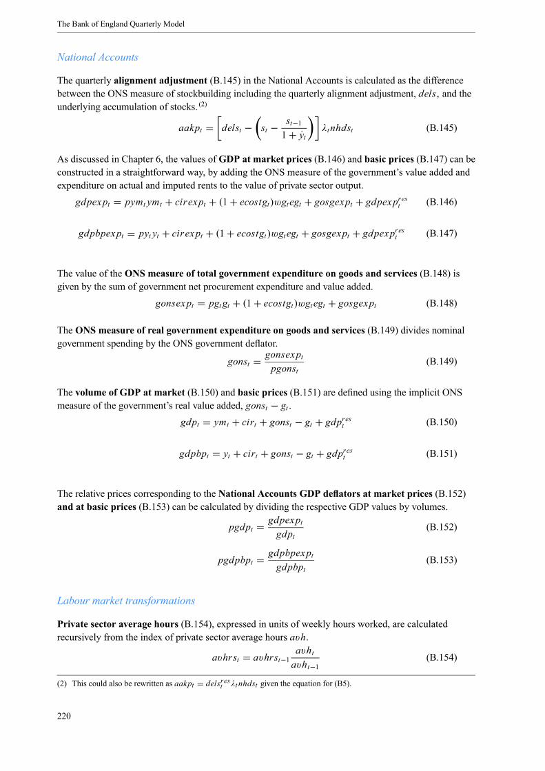
The Bank of England Quarterly Model
National Accounts
The quarterly alignment adjustment (B.145) in the National Accounts is calculated as the differencebetween the ONS measure of stockbuilding including the quarterly alignment adjustment, dels, and theunderlying accumulation of stocks. (2)
aakpt = delst − st − st−11+ yt λt nhdst (B.145)
As discussed in Chapter 6, the values of GDP at market prices (B.146) and basic prices (B.147) can beconstructed in a straightforward way, by adding the ONS measure of the government’s value added andexpenditure on actual and imputed rents to the value of private sector output.
gdpexpt = pymt ymt + cirexpt + (1+ ecostgt)wgtegt + gosgexpt + gdpexprest (B.146)
gdpbpexpt = pyt yt + cirexpt + (1+ ecostgt)wgtegt + gosgexpt + gdpexprest (B.147)
The value of the ONS measure of total government expenditure on goods and services (B.148) isgiven by the sum of government net procurement expenditure and value added.
gonsexpt = pgt gt + (1+ ecostgt)wgtegt + gosgexpt (B.148)
The ONS measure of real government expenditure on goods and services (B.149) divides nominalgovernment spending by the ONS government deflator.
gonst = gonsexptpgonst
(B.149)
The volume of GDP at market (B.150) and basic prices (B.151) are defined using the implicit ONSmeasure of the government’s real value added, gonst − gt .
gdpt = ymt + cirt + gonst − gt + gdprest (B.150)
gdpbpt = yt + cirt + gonst − gt + gdprest (B.151)
The relative prices corresponding to the National Accounts GDP deflators at market prices (B.152)and at basic prices (B.153) can be calculated by dividing the respective GDP values by volumes.
pgdpt = gdpexptgdpt
(B.152)
pgdpbpt = gdpbpexptgdpbpt
(B.153)
Labour market transformations
Private sector average hours (B.154), expressed in units of weekly hours worked, are calculatedrecursively from the index of private sector average hours avh.
avhrst = avhrst−1 avhtavht−1(B.154)
(2) This could also be rewritten as aakpt = delsrest λt nhdst given the equation for (B5).
220
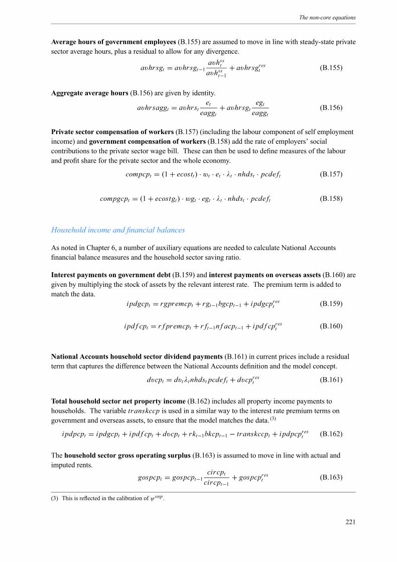
The non-core equations
Average hours of government employees (B.155) are assumed to move in line with steady-state privatesector average hours, plus a residual to allow for any divergence.
avhrsgt = avhrsgt−1 avhsst
avhsst−1+ avhrsgrest (B.155)
Aggregate average hours (B.156) are given by identity.
avhrsaggt = avhrst eteaggt
+ avhrsgt egteaggt(B.156)
Private sector compensation of workers (B.157) (including the labour component of self employmentincome) and government compensation of workers (B.158) add the rate of employers’ socialcontributions to the private sector wage bill. These can then be used to define measures of the labourand profit share for the private sector and the whole economy.
compcpt = (1+ ecostt) · wt · et · λt · nhdst · pcde ft (B.157)
compgcpt = (1+ ecostgt) · wgt · egt · λt · nhdst · pcde ft (B.158)
Household income and financial balances
As noted in Chapter 6, a number of auxiliary equations are needed to calculate National Accountsfinancial balance measures and the household sector saving ratio.
Interest payments on government debt (B.159) and interest payments on overseas assets (B.160) aregiven by multiplying the stock of assets by the relevant interest rate. The premium term is added tomatch the data.
ipdgcpt = rgpremcpt + rgt−1bgcpt−1 + i pdgcprest (B.159)
i pd f cpt = r f premcpt + r ft−1n f acpt−1 + i pd f cprest (B.160)
National Accounts household sector dividend payments (B.161) in current prices include a residualterm that captures the difference between the National Accounts definition and the model concept.
dvcpt = dvtλtnhdst pcde ft + dvcprest (B.161)
Total household sector net property income (B.162) includes all property income payments tohouseholds. The variable transkccp is used in a similar way to the interest rate premium terms ongovernment and overseas assets, to ensure that the model matches the data. (3)
i pdpcpt = i pdgcpt + i pd f cpt + dvcpt + rkt−1bkcpt−1 − transkccpt + i pdpcprest (B.162)
The household sector gross operating surplus (B.163) is assumed to move in line with actual andimputed rents.
gospcpt = gospcpt−1 circptcircpt−1+ gospcprest (B.163)
(3) This is reflected in the calibration of ψsnp.
221

The Bank of England Quarterly Model
Total government transfers to households (B.164) are the sum of unemployment benefits and othertransfer payments to households.
transbencpt = transccpt + transucpt (B.164)
Total transfer payments to households (B.165) are the sum of government transfer payments,employers’ pensions contributions and transfers from overseas.
transctcpt = transbencpt + transkpcpt + transeccpt + trans f pcpt (B.165)
Total tax payments by households (B.166) are given by the sum of income taxes, employees’ NationalInsurance Contributions, lump sum taxes and taxes on dwellings (council tax).
taxpcpt = taxwcpt + taxeecpt + taxlumpccpt + taxdcpt (B.166)
National Accounts measures of nominal (B.167) and real household consumption (B.168) arederived by adding back in actual and imputed rents to consumption. The ratio of the two is the NationalAccounts consumption deflator (B.169).
cnacpt = ccpt + circpt (B.167)
cnakpt = ckpt + cirkpt (B.168)
pcnade ft = cnacptcnakpt
(B.169)
The measure of household available resources (B.170) used to construct the ONS household savingratio includes transfers, the operating surplus, interest payments, total wages and salaries less householdtaxes. Real household resources can be obtained by dividing by the National Accounts consumptiondeflator. A residual is used to account for the conceptual differences between ONS data and BEQMvariables.
rhpikpt = 1+ rhpikprestwscpt +wsgcpt + gospcpt + transctcpt + ipdpcpt − taxpcpt
pcnade ft(B.170)
The saving ratio (B.171) is saving divided by available household resources.
savrt = pcnade ftrhpikpt − cnacptpcnade ftrhpikpt
(B.171)
Household sector net lending (B.172) is given by current saving less household investment indwellings, plus a residual to capture capital transfers and taxes.
nlpt = pcnade ftrhpikpt − cnacpt − idcpt + nlprest (B.172)
Total managed expenditure by general government (B.173) is the sum of government spending onprivate sector goods and services, government spending on factor payments, government transfers todifferent sectors and government interest payments.
tmecpt = gcpt + transccpt + transucpt + trans f cpt + transkcpt + transksubscpt+i pdgcpt + compgcpt + gosgcpt + tmecprest (B.173)
222

The non-core equations
General government net lending (B.174) is the difference between total tax revenues and totalmanaged expenditure. General government net borrowing (B.175) is the reverse.
nlggt = taxcpt − tmecpt + nlggrest (B.174)
ggnbcpt = tmecpt − taxcpt + ggnbcprest (B.175)
Overseas net lending (B.176) is the reverse of the current account of the balance of payments plus netcapital transfers.
nl ft = −xmcacpt + nl f rest (B.176)
223


Appendix C Data transformations and sources
This appendix lists the data transformations and sources for BEQM variables. As set out in Chapter 6,BEQM data are transformed into ‘model units’ and then transformed out again into levels. Most of thesources are either another BEQM variable or an original source – unless otherwise indicated, this is thecode from the Office for National Statistics database (four letter identifiers shown in capitals). Anasterisk indicates that some of the backdata for the series have been constructed, and the source used forthis is indicated in the third column. To ease the exposition, a few additional variables are included herethat do not feature in the model equations reported above – for example, aggregate wages and salaries(wsagg) appears in the expression for post-tax labour income (ly) and as the denominator for someeffective tax rates.
Tables 6.1 and 6.2 illustrate the notation we use for data, actual units and detrended model units. ABEQM quantity variable can have up to four associated concepts. To avoid confusion with ONSdatabase identifiers and to help distinguish between the related concepts, we use lower case italicnotation for most BEQM variables as follows:• volume measure in detrended model units;• current price (nominal) measure, with suffix cp;• chained volume measure (CVM), with suffix kp; and• (implicit) price deflator, with suffix def.
For some prices, we also calculated the associated inflation rate, usually quarterly, which we denoteeither by a dot above the variable or (for longer names) by the suffix dot.
The BEQM variables that are not in lower case italics are generally parameters, shown as Greek letters.Most monetary variables here are in terms of £ million. Chained volume measures are in the prices ofthe reference year, currently 2001.
Table C.1: Data sources and transformations for BEQM
NAME DESCRIPTION CALCULATIONaacp Alignment adjustment, current prices DMUNaakp Alignment adjustment, CVM DMUMacp Net financial wealth of household
sector, current pricesNZEA (*ALDZ)
avh Index of private sector average hours(1995=1)
avhrs/avhrs[1995 value]
avhrs Average weekly hours worked in theprivate sector
BoE constructed data, derived from LFSmicrodata
avhrsagg Average weekly hours worked in thewhole economy
1000·eagghrs/eagghds
avhrsg Average weekly hours worked in thegeneral government sector
1000·eghrs/eghds
ben Unemployment benefits, detrendedmodel units
transucp/(λ·uhds·pcdef )
225
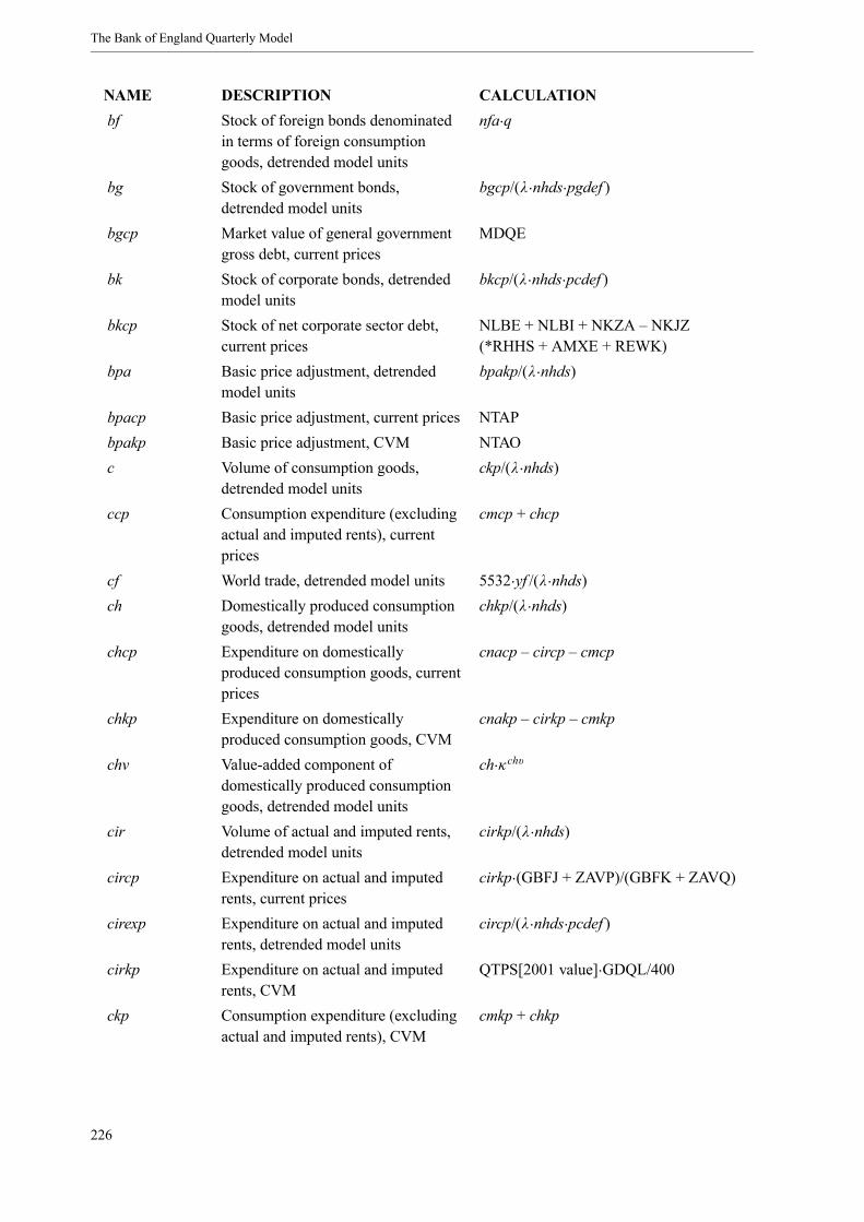
The Bank of England Quarterly Model
NAME DESCRIPTION CALCULATIONbf Stock of foreign bonds denominated
in terms of foreign consumptiongoods, detrended model units
nfa·q
bg Stock of government bonds,detrended model units
bgcp/(λ·nhds·pgdef )
bgcp Market value of general governmentgross debt, current prices
MDQE
bk Stock of corporate bonds, detrendedmodel units
bkcp/(λ·nhds·pcdef )
bkcp Stock of net corporate sector debt,current prices
NLBE + NLBI + NKZA – NKJZ(*RHHS + AMXE + REWK)
bpa Basic price adjustment, detrendedmodel units
bpakp/(λ·nhds)
bpacp Basic price adjustment, current prices NTAPbpakp Basic price adjustment, CVM NTAOc Volume of consumption goods,
detrended model unitsckp/(λ·nhds)
ccp Consumption expenditure (excludingactual and imputed rents), currentprices
cmcp + chcp
cf World trade, detrended model units 5532·yf /(λ·nhds)ch Domestically produced consumption
goods, detrended model unitschkp/(λ·nhds)
chcp Expenditure on domesticallyproduced consumption goods, currentprices
cnacp – circp – cmcp
chkp Expenditure on domesticallyproduced consumption goods, CVM
cnakp – cirkp – cmkp
chv Value-added component ofdomestically produced consumptiongoods, detrended model units
ch·κchv
cir Volume of actual and imputed rents,detrended model units
cirkp/(λ·nhds)
circp Expenditure on actual and imputedrents, current prices
cirkp·(GBFJ + ZAVP)/(GBFK + ZAVQ)
cirexp Expenditure on actual and imputedrents, detrended model units
circp/(λ·nhds·pcdef )
cirkp Expenditure on actual and imputedrents, CVM
QTPS[2001 value]·GDQL/400
ckp Consumption expenditure (excludingactual and imputed rents), CVM
cmkp + chkp
226
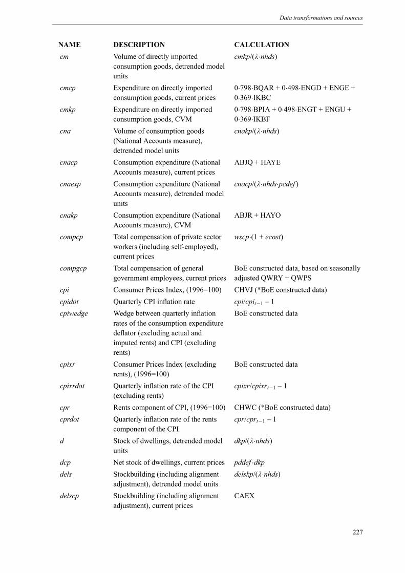
Data transformations and sources
NAME DESCRIPTION CALCULATIONcm Volume of directly imported
consumption goods, detrended modelunits
cmkp/(λ·nhds)
cmcp Expenditure on directly importedconsumption goods, current prices
0·798·BQAR + 0·498·ENGD + ENGE +0·369·IKBC
cmkp Expenditure on directly importedconsumption goods, CVM
0·798·BPIA + 0·498·ENGT + ENGU +0·369·IKBF
cna Volume of consumption goods(National Accounts measure),detrended model units
cnakp/(λ·nhds)
cnacp Consumption expenditure (NationalAccounts measure), current prices
ABJQ + HAYE
cnaexp Consumption expenditure (NationalAccounts measure), detrended modelunits
cnacp/(λ·nhds·pcdef )
cnakp Consumption expenditure (NationalAccounts measure), CVM
ABJR + HAYO
compcp Total compensation of private sectorworkers (including self-employed),current prices
wscp·(1 + ecost)
compgcp Total compensation of generalgovernment employees, current prices
BoE constructed data, based on seasonallyadjusted QWRY + QWPS
cpi Consumer Prices Index, (1996=100) CHVJ (*BoE constructed data)cpidot Quarterly CPI inflation rate cpi/cpit−1 – 1cpiwedge Wedge between quarterly inflation
rates of the consumption expendituredeflator (excluding actual andimputed rents) and CPI (excludingrents)
BoE constructed data
cpixr Consumer Prices Index (excludingrents), (1996=100)
BoE constructed data
cpixrdot Quarterly inflation rate of the CPI(excluding rents)
cpixr/cpixrt−1 – 1
cpr Rents component of CPI, (1996=100) CHWC (*BoE constructed data)cprdot Quarterly inflation rate of the rents
component of the CPIcpr/cprt−1 – 1
d Stock of dwellings, detrended modelunits
dkp/(λ·nhds)
dcp Net stock of dwellings, current prices pddef ·dkpdels Stockbuilding (including alignment
adjustment), detrended model unitsdelskp/(λ·nhds)
delscp Stockbuilding (including alignmentadjustment), current prices
CAEX
227
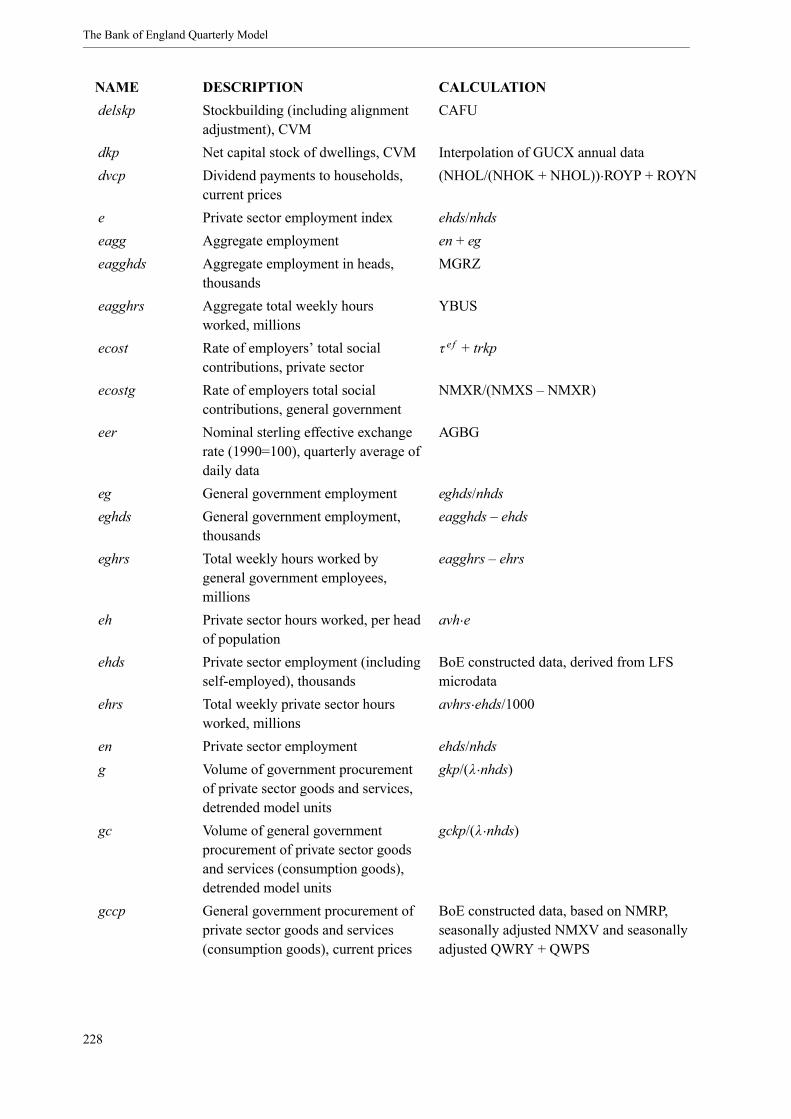
The Bank of England Quarterly Model
NAME DESCRIPTION CALCULATIONdelskp Stockbuilding (including alignment
adjustment), CVMCAFU
dkp Net capital stock of dwellings, CVM Interpolation of GUCX annual datadvcp Dividend payments to households,
current prices(NHOL/(NHOK + NHOL))·ROYP + ROYN
e Private sector employment index ehds/nhdseagg Aggregate employment en + egeagghds Aggregate employment in heads,
thousandsMGRZ
eagghrs Aggregate total weekly hoursworked, millions
YBUS
ecost Rate of employers’ total socialcontributions, private sector
τ e f + trkp
ecostg Rate of employers total socialcontributions, general government
NMXR/(NMXS – NMXR)
eer Nominal sterling effective exchangerate (1990=100), quarterly average ofdaily data
AGBG
eg General government employment eghds/nhdseghds General government employment,
thousandseagghds – ehds
eghrs Total weekly hours worked bygeneral government employees,millions
eagghrs – ehrs
eh Private sector hours worked, per headof population
avh·e
ehds Private sector employment (includingself-employed), thousands
BoE constructed data, derived from LFSmicrodata
ehrs Total weekly private sector hoursworked, millions
avhrs·ehds/1000
en Private sector employment ehds/nhdsg Volume of government procurement
of private sector goods and services,detrended model units
gkp/(λ·nhds)
gc Volume of general governmentprocurement of private sector goodsand services (consumption goods),detrended model units
gckp/(λ·nhds)
gccp General government procurement ofprivate sector goods and services(consumption goods), current prices
BoE constructed data, based on NMRP,seasonally adjusted NMXV and seasonallyadjusted QWRY + QWPS
228

Data transformations and sources
NAME DESCRIPTION CALCULATIONgckp General government procurement of
private sector goods and services(consumption goods), CVM
gccp/pgcdef
gconscp ONS-measured general governmentfinal consumption expenditure,current prices
NMRP
gconskp ONS-measured general governmentfinal consumption expenditure, CVM
NMRY
gcp General government procurement ofprivate sector goods and services,current prices
gccp + igcp
gdp Volume of GDP at market prices,detrended model units
gdpkp/(λ·nhds)
gdpbp Volume of GDP at basic prices,detrended model units
gdpbpkp/(λ·nhds)
gdpbpcp GDP at basic prices, current prices gdpcp – bpacpgdpbpexp Value of GDP at basic prices,
detrended model unitsgdpbpcp/(λ·nhds·pcdef )
gdpbpkp GDP at basic prices, CVM ABMMgdpcp GDP at market prices, current prices YBHAgdpexp Value of GDP at market prices,
detrended model unitsgdpcp/(λ·nhds·pcdef )
gdpkp GDP at market prices, CVM ABMIggnbcp General government net borrowing,
current pricestmecp – taxcp
gkp Total general governmentprocurement of private sector goodsand services, CVM
gckp + igkp
gons Volume of total ONS-measuredgeneral government finalconsumption and investmentexpenditure, detrended model units
gonskp/(λ·nhds)
gonscp Total ONS-measured generalgovernment final consumption andinvestment expenditure, currentprices
gconscp + igcp
gonskp Total ONS-measured generalgovernment final consumption andinvestment expenditure, CVM
gconskp + igkp
gosgcp General government gross operatingsurplus, current prices
gconscp – compgcp – gccp
gosgexp General government gross operatingsurplus, detrended model units
gosgcp/(λ·nhds·pcdef )
229

The Bank of England Quarterly Model
NAME DESCRIPTION CALCULATIONgospcp Household sector gross operating
surplus, current pricesCAEN
gv Value-added component of totalgeneral government procurement,detrended model units
g·κgv
id Volume of investment in dwellings,detrended model units
idkp/(λ·nhds)
idcp Private sector investment indwellings, current prices
GGAG
idkp Private sector investment indwellings, CVM
DFEA
ig Volume of government procurementof investment goods, detrendedmodel units
igkp/(λ·nhds)
igcp General government procurement ofprivate sector goods and services(capital goods), current prices
RPZG (*seasonally adjusted AAYE)
igkp General government procurement ofprivate sector goods and services(capital goods), CVM
DLWF (*DFED)
ik Volume of total business investment,detrended model units
ikkp/(λ·nhds)
ikcp Business investment, current prices NPEKikexp Total business investment
expenditure, detrended model unitsikcp/(λ·nhds·pcdef )
ikh Volume of domestically producedinvestment, detrended model units
ikhkp/(λ·nhds)
ikhcp Business investment (domesticallyproduced), current prices
ikcp – ikmcp
ikhkp Business investment (domesticallyproduced), CVM
ikkp – ikmkp
ikhv Value-added component ofdomestically produced investment,detrended model units
ikh·κ ikhv
ikkp Business investment, CVM NPELikm Volume of directly imported
investment, detrended model unitsikmkp/(λ·nhds)
ikmcp Business investment (directlyimported), current prices
ENGG
ikmkp Business investment (directlyimported), CVM
ENGW
io Volume of other investment,detrended model units
iokp/(λ·nhds)
230
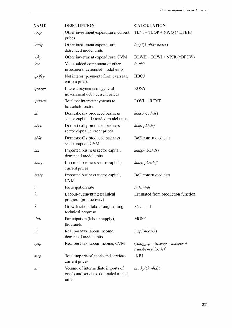
Data transformations and sources
NAME DESCRIPTION CALCULATIONiocp Other investment expenditure, current
pricesTLNI + TLOP + NPJQ (* DFBH)
ioexp Other investment expenditure,detrended model units
iocp/(λ·nhds·pcdef )
iokp Other investment expenditure, CVM DLWH + DLWI + NPJR (*DFDW)iov Value-added component of other
investment, detrended model unitsio·κ iov
ipdfcp Net interest payments from overseas,current prices
HBOJ
ipdgcp Interest payments on generalgovernment debt, current prices
ROXY
ipdpcp Total net interest payments tohousehold sector
ROYL – ROYT
kh Domestically produced businesssector capital, detrended model units
khkp/(λ·nhds)
khcp Domestically produced businesssector capital, current prices
khkp·pkhdef
khkp Domestically produced businesssector capital, CVM
BoE constructed data
km Imported business sector capital,detrended model units
kmkp/(λ·nhds)
kmcp Imported business sector capital,current prices
kmkp·pkmdef
kmkp Imported business sector capital,CVM
BoE constructed data
l Participation rate lhds/nhdsλ Labour-augmenting technical
progress (productivity)Estimated from production function
λ Growth rate of labour-augmentingtechnical progress
λ/λt−1 – 1
lhds Participation (labour supply),thousands
MGSF
ly Real post-tax labour income,detrended model units
lykp/(nhds·λ)
lykp Real post-tax labour income, CVM (wsaggcp – taxwcp – taxeecp +transbencp)/pcdef
mcp Total imports of goods and services,current prices
IKBI
mi Volume of intermediate imports ofgoods and services, detrended modelunits
minkp/(λ·nhds)
231
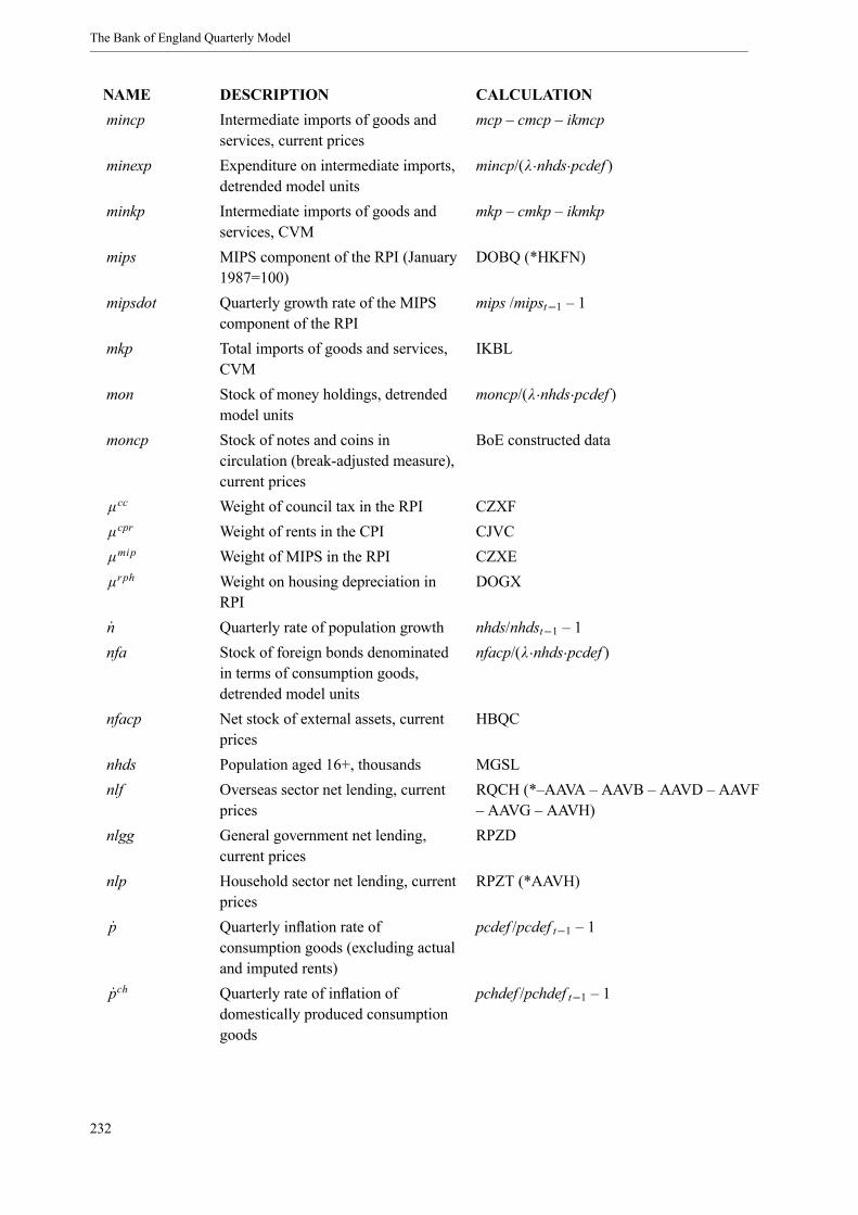
The Bank of England Quarterly Model
NAME DESCRIPTION CALCULATIONmincp Intermediate imports of goods and
services, current pricesmcp – cmcp – ikmcp
minexp Expenditure on intermediate imports,detrended model units
mincp/(λ·nhds·pcdef )
minkp Intermediate imports of goods andservices, CVM
mkp – cmkp – ikmkp
mips MIPS component of the RPI (January1987=100)
DOBQ (*HKFN)
mipsdot Quarterly growth rate of the MIPScomponent of the RPI
mips /mipst−1 – 1
mkp Total imports of goods and services,CVM
IKBL
mon Stock of money holdings, detrendedmodel units
moncp/(λ·nhds·pcdef )
moncp Stock of notes and coins incirculation (break-adjusted measure),current prices
BoE constructed data
µcc Weight of council tax in the RPI CZXFµcpr Weight of rents in the CPI CJVCµmip Weight of MIPS in the RPI CZXEµrph Weight on housing depreciation in
RPIDOGX
n Quarterly rate of population growth nhds/nhdst−1 – 1nfa Stock of foreign bonds denominated
in terms of consumption goods,detrended model units
nfacp/(λ·nhds·pcdef )
nfacp Net stock of external assets, currentprices
HBQC
nhds Population aged 16+, thousands MGSLnlf Overseas sector net lending, current
pricesRQCH (*–AAVA – AAVB – AAVD – AAVF– AAVG – AAVH)
nlgg General government net lending,current prices
RPZD
nlp Household sector net lending, currentprices
RPZT (*AAVH)
p Quarterly inflation rate ofconsumption goods (excluding actualand imputed rents)
pcdef /pcdef t−1 – 1
pch Quarterly rate of inflation ofdomestically produced consumptiongoods
pchdef /pchdef t−1 – 1
232
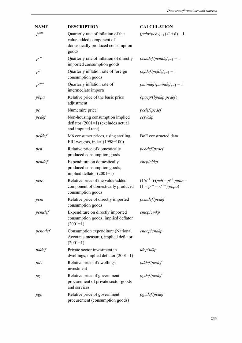
Data transformations and sources
NAME DESCRIPTION CALCULATIONpchv Quarterly rate of inflation of the
value-added component ofdomestically produced consumptiongoods
(pchv/pchvt−1)·(1+ p) – 1
pcm Quarterly rate of inflation of directlyimported consumption goods
pcmdef /pcmdef t−1 – 1
p f Quarterly inflation rate of foreignconsumption goods
pcfdef /pcfdef t−1 – 1
pmin Quarterly inflation rate ofintermediate imports
pmindef /pmindef t−1 – 1
pbpa Relative price of the basic priceadjustment
bpacp/(bpakp·pcdef )
pc Numeraire price pcdef /pcdefpcdef Non-housing consumption implied
deflator (2001=1) (excludes actualand imputed rent)
ccp/ckp
pcfdef M6 consumer prices, using sterlingERI weights, index (1998=100)
BoE constructed data
pch Relative price of domesticallyproduced consumption goods
pchdef /pcdef
pchdef Expenditure on domesticallyproduced consumption goods,implied deflator (2001=1)
chcp/chkp
pchv Relative price of the value-addedcomponent of domestically producedconsumption goods
(1/κchv)·(pch – ρch·pmin –(1 – ρch – κchv )·pbpa)
pcm Relative price of directly importedconsumption goods
pcmdef /pcdef
pcmdef Expenditure on directly importedconsumption goods, implied deflator(2001=1)
cmcp/cmkp
pcnadef Consumption expenditure (NationalAccounts measure), implied deflator(2001=1)
cnacp/cnakp
pddef Private sector investment indwellings, implied deflator (2001=1)
idcp/idkp
pdv Relative price of dwellingsinvestment
pddef /pcdef
pg Relative price of governmentprocurement of private sector goodsand services
pgdef /pcdef
pgc Relative price of governmentprocurement (consumption goods)
pgcdef /pcdef
233
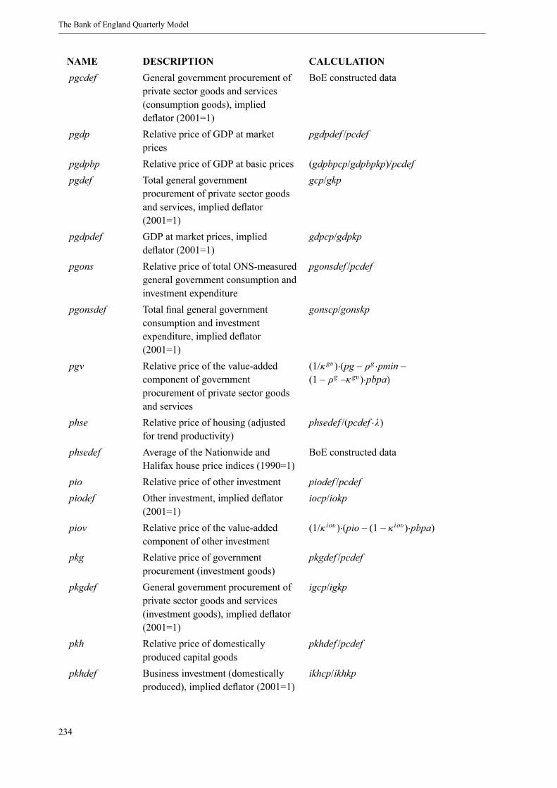
The Bank of England Quarterly Model
NAME DESCRIPTION CALCULATIONpgcdef General government procurement of
private sector goods and services(consumption goods), implieddeflator (2001=1)
BoE constructed data
pgdp Relative price of GDP at marketprices
pgdpdef /pcdef
pgdpbp Relative price of GDP at basic prices (gdpbpcp/gdpbpkp)/pcdefpgdef Total general government
procurement of private sector goodsand services, implied deflator(2001=1)
gcp/gkp
pgdpdef GDP at market prices, implieddeflator (2001=1)
gdpcp/gdpkp
pgons Relative price of total ONS-measuredgeneral government consumption andinvestment expenditure
pgonsdef /pcdef
pgonsdef Total final general governmentconsumption and investmentexpenditure, implied deflator(2001=1)
gonscp/gonskp
pgv Relative price of the value-addedcomponent of governmentprocurement of private sector goodsand services
(1/κgv )·(pg – ρg·pmin –(1 – ρg –κgv )·pbpa)
phse Relative price of housing (adjustedfor trend productivity)
phsedef /(pcdef ·λ)
phsedef Average of the Nationwide andHalifax house price indices (1990=1)
BoE constructed data
pio Relative price of other investment piodef /pcdefpiodef Other investment, implied deflator
(2001=1)iocp/iokp
piov Relative price of the value-addedcomponent of other investment
(1/κ iov )·(pio – (1 – κ iov )·pbpa)
pkg Relative price of governmentprocurement (investment goods)
pkgdef /pcdef
pkgdef General government procurement ofprivate sector goods and services(investment goods), implied deflator(2001=1)
igcp/igkp
pkh Relative price of domesticallyproduced capital goods
pkhdef /pcdef
pkhdef Business investment (domesticallyproduced), implied deflator (2001=1)
ikhcp/ikhkp
234
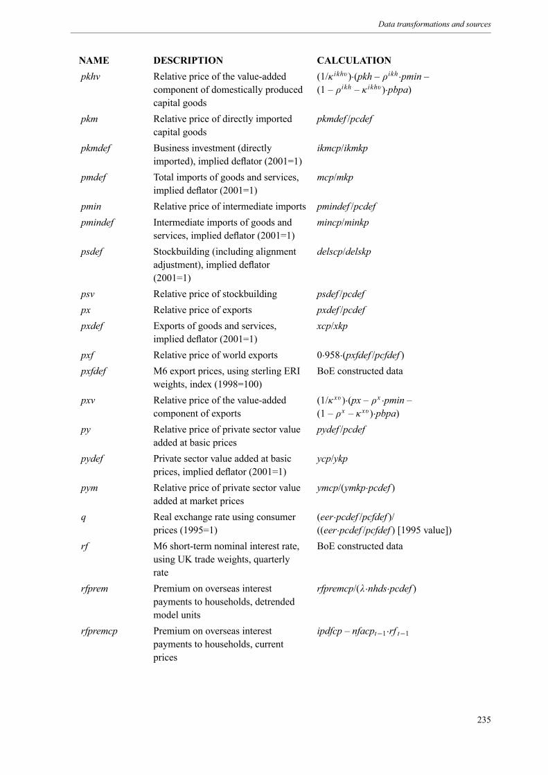
Data transformations and sources
NAME DESCRIPTION CALCULATIONpkhv Relative price of the value-added
component of domestically producedcapital goods
(1/κ ikhv )·(pkh – ρikh·pmin –(1 – ρikh – κ ikhv )·pbpa)
pkm Relative price of directly importedcapital goods
pkmdef /pcdef
pkmdef Business investment (directlyimported), implied deflator (2001=1)
ikmcp/ikmkp
pmdef Total imports of goods and services,implied deflator (2001=1)
mcp/mkp
pmin Relative price of intermediate imports pmindef /pcdefpmindef Intermediate imports of goods and
services, implied deflator (2001=1)mincp/minkp
psdef Stockbuilding (including alignmentadjustment), implied deflator(2001=1)
delscp/delskp
psv Relative price of stockbuilding psdef /pcdefpx Relative price of exports pxdef /pcdefpxdef Exports of goods and services,
implied deflator (2001=1)xcp/xkp
pxf Relative price of world exports 0·958·(pxfdef /pcfdef )pxfdef M6 export prices, using sterling ERI
weights, index (1998=100)BoE constructed data
pxv Relative price of the value-addedcomponent of exports
(1/κ xv )·(px – ρx ·pmin –(1 – ρx – κ xv )·pbpa)
py Relative price of private sector valueadded at basic prices
pydef /pcdef
pydef Private sector value added at basicprices, implied deflator (2001=1)
ycp/ykp
pym Relative price of private sector valueadded at market prices
ymcp/(ymkp·pcdef )
q Real exchange rate using consumerprices (1995=1)
(eer·pcdef /pcfdef )/((eer·pcdef /pcfdef ) [1995 value])
rf M6 short-term nominal interest rate,using UK trade weights, quarterlyrate
BoE constructed data
rfprem Premium on overseas interestpayments to households, detrendedmodel units
rfpremcp/(λ·nhds·pcdef )
rfpremcp Premium on overseas interestpayments to households, currentprices
ipdfcp – nfacpt−1·rf t−1
235

The Bank of England Quarterly Model
NAME DESCRIPTION CALCULATIONrg Short-term nominal interest rate,
quarterly rate((1 + (rga/100)) 14 – 1)
rga Short-term nominal interest rate,annual rate, per cent
AMIH
rgprem Premium on government interestpayments to households, detrendedmodel units
rgpremcp/(λ·nhds·pcdef )
rgpremcp Premium on government interestpayments to households, currentprices
(ipdgcp – rgt−1·bgcpt−1)
rhpikp Total available household resources,CVM
(RPHQ + RPQJ)·cnakp/cnacp
rpcc Council tax component of the RPI DOBR (*HFKO)rpccdot Quarterly inflation rate of the council
tax component of the RPIrpcc/rpcct−1 – 1
rph Housing depreciation component ofthe RPI, (January 1995=100)
CHOO
rphdot Quarterly inflation rate of the housingdepreciation component of the RPI
rph/rpht−1 – 1
rpi Retail Prices Index (January1987=100)
CHAW (*CBAB)
rpidot Quarterly inflation rate of the RPI rpi/rpit−1 – 1rpidotsa Quarterly inflation rate of the RPI,
seasonally adjustedBoE constructed data
rpix Retail Prices Index excludingmortgage interest payments (January1987=100)
CHMK (*RYYW)
rpixdot Quarterly inflation rate of RPIX rpix/rpixt−1 – 1rpixwedge Wedge between quarterly growth rate
of the RPI, excluding council tax andhousing depreciation and the CPI,excluding rents
BoE constructed data
rpxc Retail Prices Index excludingmortgage interest payments andcouncil tax (January 1987=100)
DQAD
rpxcdot Quarterly inflation rate of the RPI,excluding mortgage interestpayments and council tax
rpxc/rpxct−1 – 1
rpxch Retail Prices Index, excluding MIPS,council tax and housing depreciation(January 1987=100)
BoE constructed data
236

Data transformations and sources
NAME DESCRIPTION CALCULATIONrpxchdot Quarterly inflation rate of RPI,
excluding MIPS, council tax andhousing depreciation
rpxch/rpxcht−1 – 1
s Stock of inventories, detrended modelunits
skp/(λ·nhds)
savr Household sector saving ratio, percent
100·(1 – cnakp/rhpikp)
sd Statistical discrepancy, detrendedmodel units
sdkp/(λ·nhds)
sdcp Statistical discrepancy, current prices GIXMsdexp Value of statistical discrepancy,
detrended model unitssdcp/(λ·nhds·pcdef )
sdkp Statistical discrepancy, CVM GIXSskp Stock of inventories, CVM BoE constructed dataτ c Effective net indirect tax rate (ratio of
basic price adjustment to valueadded)
bpacp/ycp
τ d Effective tax rate on dwellings taxdcp/dcpτ ee Effective rate of employees’ National
Insurance Contributionstaxeecp/wsaggcp
τ e f Effective rate of employers’ NationalInsurance Contributions
taxefcp/wsaggcp
τ eu Effective tax rate on EU net indirecttaxes
taxeucp/ycp
τ f Effective tax rate on revenue fromoverseas residents
taxfcp/ycp
τ knd Effective corporation tax rate taxkcp/ycpτ lumpc Effective lump sum tax rate on
householdstaxlumpccp/ycp
τ lumpk Effective lump sum tax rate on firms taxlumpkcp/ycpτw Effective income tax rate taxwcp/wsaggcptax Total taxation receipts, detrended
model unitstaxcp/(λ·nhds·pcdef )
taxcp Total taxation receipts, current prices GZXXtaxd Tax revenue from tax on dwellings,
detrended model unitstaxdcp/(λ·nhds·pcdef )
taxdcp Tax revenue from tax on dwellings(council tax), current prices
RNTO
taxee Employees’ National InsuranceContributions, detrended model units
taxeecp/(λ·nhds·pcdef )
taxeecp Employees’ National InsuranceContributions, current prices
AIIV – CUCT
237

The Bank of England Quarterly Model
NAME DESCRIPTION CALCULATIONtaxef Employers’ National Insurance
Contributions, detrended model unitstaxefcp/(λ·nhds·pcdef )
taxefcp Employers’ National InsuranceContributions, current prices
CUCT
taxeu Indirect taxes minus subsidies paid toEU, detrended model units
taxeucp/(λ·nhds·pcdef )
taxeucp Indirect taxes minus subsidies paid toEU, current prices
CGDR – FKNG (*FJWB – FJWJ)
taxf Tax revenue from overseas residents,detrended model units
taxfcp/(λ·nhds·pcdef )
taxfcp Tax revenue from overseas residents,current prices
FHDM (*FJKI + FKKL)
taxind Tax revenue from indirect taxation,detrended model units
taxindcp/(λ·nhds·pcdef )
taxindcp Tax revenue from indirect taxation,current prices
bpacp + transksubscp – taxeucp
taxk Tax revenue from corporation tax,detrended model units
taxkcp/(λ·nhds·pcdef )
taxkcp Tax revenue from corporation tax,current prices
Seasonally adjusted ACCJ + ACCD + EYNK(*AIAY + AIFS + ADRV)
taxlumpc Tax revenue from lump sum taxes onhouseholds, detrended model units
taxlumpccp/(λ·nhds·pcdef )
taxlumpccp Tax revenue from lump sum taxes onhouseholds, current prices
RNGQ + RPHT – RNTO (*RNGQ + CFGE)
taxlumpk Tax revenue from lump sum taxes onfirms, detrended model units
taxlumpkcp/(λ·nhds·pcdef )
taxlumpkcp Tax revenue from lump sum taxes onfirms, current prices
taxcp – taxwcp – taxindcp – taxlumpccp –taxkcp – taxfcp – taxdcp – taxeecp – taxefcp –gosgcp
taxpcp Total tax payments of householdsector, current prices
taxwcp + taxeecp + taxlumpccp + taxdcp
taxw Tax revenue from labour incometaxes, detrended model units
taxwcp/(λ·nhds·pcdef )
taxwcp Tax revenue from labour incometaxes, current prices
RPHS (*AIIU)
tmecp Total managed general governmentexpenditure, current prices
GZWA + NMXO – EQJW
trans Total general government transfers,detrended model units
transc + transu + transk + transf + transksubs+ rgprem
transbencp Total general government transferpayments to households, currentprices
GZVX
238

Data transformations and sources
NAME DESCRIPTION CALCULATIONtransc General government transfer
payments to households excludingunemployment benefit, detrendedmodel units
transccp/(λ·nhds·pcdef )
transccp General government transferpayments to households excludingunemployment benefit, current prices
transbencp – transucp
transctcp Total transfer payments tohouseholds, current prices
transbencp + transkpcp + transfpcp +transeccp
transec Employers’ private socialcontributions, general government,detrended model units
transeccp/(λ·nhds·pcdef )
transeccp Employers’ private socialcontributions, general government,current prices
wsgcp·trec
transf General government transfers tooverseas sector, detrended modelunits
transfcp/(λ·nhds·pcdef )
transfcp General government transfers tooverseas sector, current prices
FLUD – FNTL (*BoE constructed)
transfp Net overseas transfers to households,detrended model units
transfpcp/(λ·nhds·pcdef )
transfpcp Net overseas transfers to households,current prices
FNTP + FKIL – FKIQ
transk General government transfers tofirms, detrended model units
transkcp/(λ·nhds·pcdef )
transkc Supernormal profit transfers fromfirms to households, detrended modelunits
transkccp/(λ·nhds·pcdef )
transkccp Supernormal profit transfers fromfirms to households, current prices
-(ROYM + ROYQ – ROYU – ROYV +(NHOK/(NHOK + NHOL))·ROYP – ipdfcp –ipdgcp – rkt−1·bkcpt−1)
transkcp General government transfers tofirms, current prices
tmecp – gcp – transccp – transucp – transfcp– transksubscp – ipdgcp – compgcp – gosgcp
transkf Net transfers from firms to overseas,detrended model units
transkfcp/(λ·nhds·pcdef )
transkfcp Net transfers from firms to overseas,current prices
–FNTC – CGDR + FKNG – FNTQ – FNTR –FNTS + FKIL – FKIQ
transkp Employers’ other socialcontributions, private sector,detrended model units
transkpcp/(λ·nhds·pcdef )
239

The Bank of England Quarterly Model
NAME DESCRIPTION CALCULATIONtranskpcp Employers’ other social
contributions, private sector, currentprices
ROYK – transeccp – taxefcp
transksubs General government subsidies onproducts, detrended model units
transksubscp/(λ·nhds·pcdef )
transksubscp General government subsidies onproducts, current prices
NTAG – NTAP – FKNG(*NTAG – NTAP – seasonally adjusted FJWJ)
transu Total unemployment benefits,detrended model units
transucp/(λ·nhds·pcdef )
transucp Total unemployment benefits, currentprices
µbenw·u·lhds·wdef
trc General government transfer rate tohouseholds (excludingunemployment benefit)
transccp/ycp
trec Rate of employers’ other socialcontributions, general government
ecostg – τ e f
trf General government transfer rate toforeigners
transfcp/ycp
trfp Rate of net transfers from foreignersto households
transfpcp/ycp
trk General government transfer rate tofirms
transkcp/ycp
trkf Transfer rate from firms to overseas transkfcp/ycptrkp Transfer rate from firms to
householdstranskpcp/wscp
trksubs Subsidy rate from generalgovernment to firms
transksubscp/ycp
u Unemployment rate uhds/lhdsuhds Unemployment, thousands MGSCulc Private sector unit labour costs wdef ·(1 + ecost)/prodhdsur Unemployment rate, per cent 100·uv Value of equities, detrended model
unitsvcp/(λ·nhds·pcdef )
vcp Nominal value of equities, currentprices
acp – bgcp – bkcp – nfacp – moncp
w Private sector real wage, detrendedmodel units
wdef /(λ·pcdef )
w Quarterly growth rate of nominalprivate sector wages
wdef /wdef t−1 – 1
wagg Aggregate real wage, detrendedmodel units
waggdef /(λ·pcdef )
240
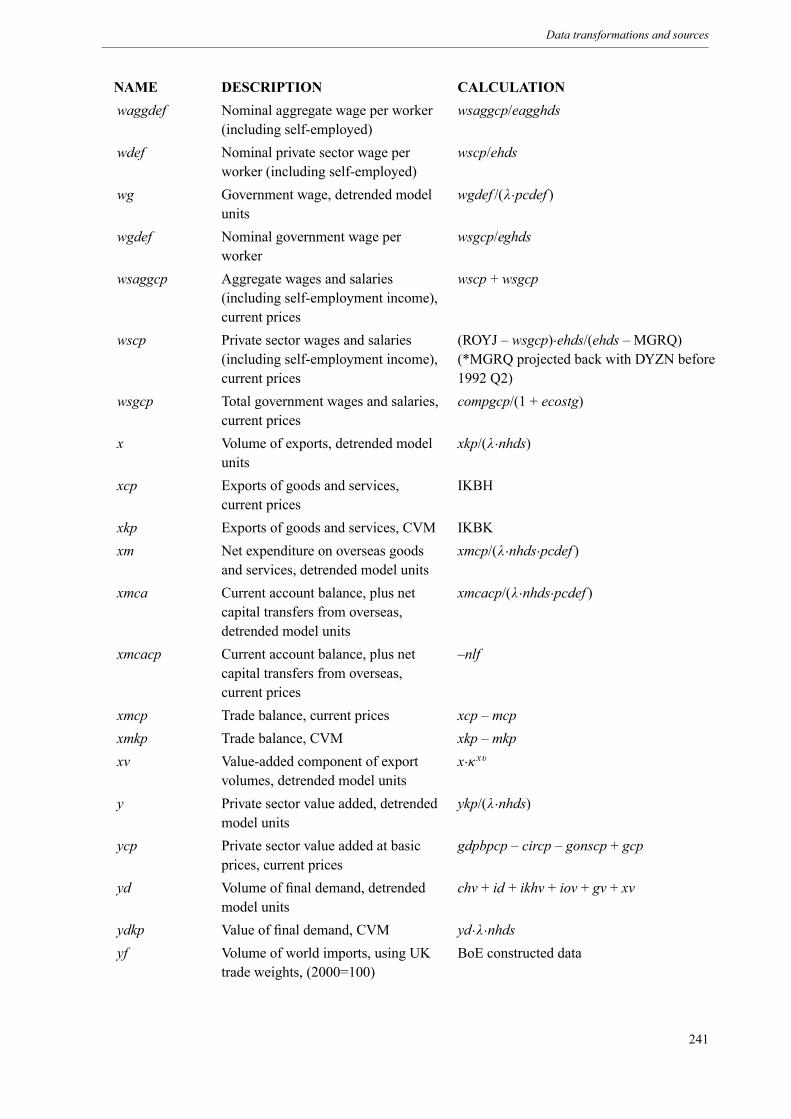
Data transformations and sources
NAME DESCRIPTION CALCULATIONwaggdef Nominal aggregate wage per worker
(including self-employed)wsaggcp/eagghds
wdef Nominal private sector wage perworker (including self-employed)
wscp/ehds
wg Government wage, detrended modelunits
wgdef /(λ·pcdef )
wgdef Nominal government wage perworker
wsgcp/eghds
wsaggcp Aggregate wages and salaries(including self-employment income),current prices
wscp + wsgcp
wscp Private sector wages and salaries(including self-employment income),current prices
(ROYJ – wsgcp)·ehds/(ehds – MGRQ)(*MGRQ projected back with DYZN before1992 Q2)
wsgcp Total government wages and salaries,current prices
compgcp/(1 + ecostg)
x Volume of exports, detrended modelunits
xkp/(λ·nhds)
xcp Exports of goods and services,current prices
IKBH
xkp Exports of goods and services, CVM IKBKxm Net expenditure on overseas goods
and services, detrended model unitsxmcp/(λ·nhds·pcdef )
xmca Current account balance, plus netcapital transfers from overseas,detrended model units
xmcacp/(λ·nhds·pcdef )
xmcacp Current account balance, plus netcapital transfers from overseas,current prices
–nlf
xmcp Trade balance, current prices xcp – mcpxmkp Trade balance, CVM xkp – mkpxv Value-added component of export
volumes, detrended model unitsx·κ xv
y Private sector value added, detrendedmodel units
ykp/(λ·nhds)
ycp Private sector value added at basicprices, current prices
gdpbpcp – circp – gonscp + gcp
yd Volume of final demand, detrendedmodel units
chv + id + ikhv + iov + gv + xv
ydkp Value of final demand, CVM yd·λ·nhdsyf Volume of world imports, using UK
trade weights, (2000=100)BoE constructed data
241

The Bank of England Quarterly Model
NAME DESCRIPTION CALCULATIONykp Private sector value added at basic
prices, CVMgdpbpkp – cirkp – gonskp + gkp
ym Private sector value added at marketprices, detrended model units
ymkp/(λ·nhds)
ymcp Private sector value added at marketprices, current prices
ycp + bpacp
ymkp Private sector value added at marketprices, CVM
ykp + bpakp
242
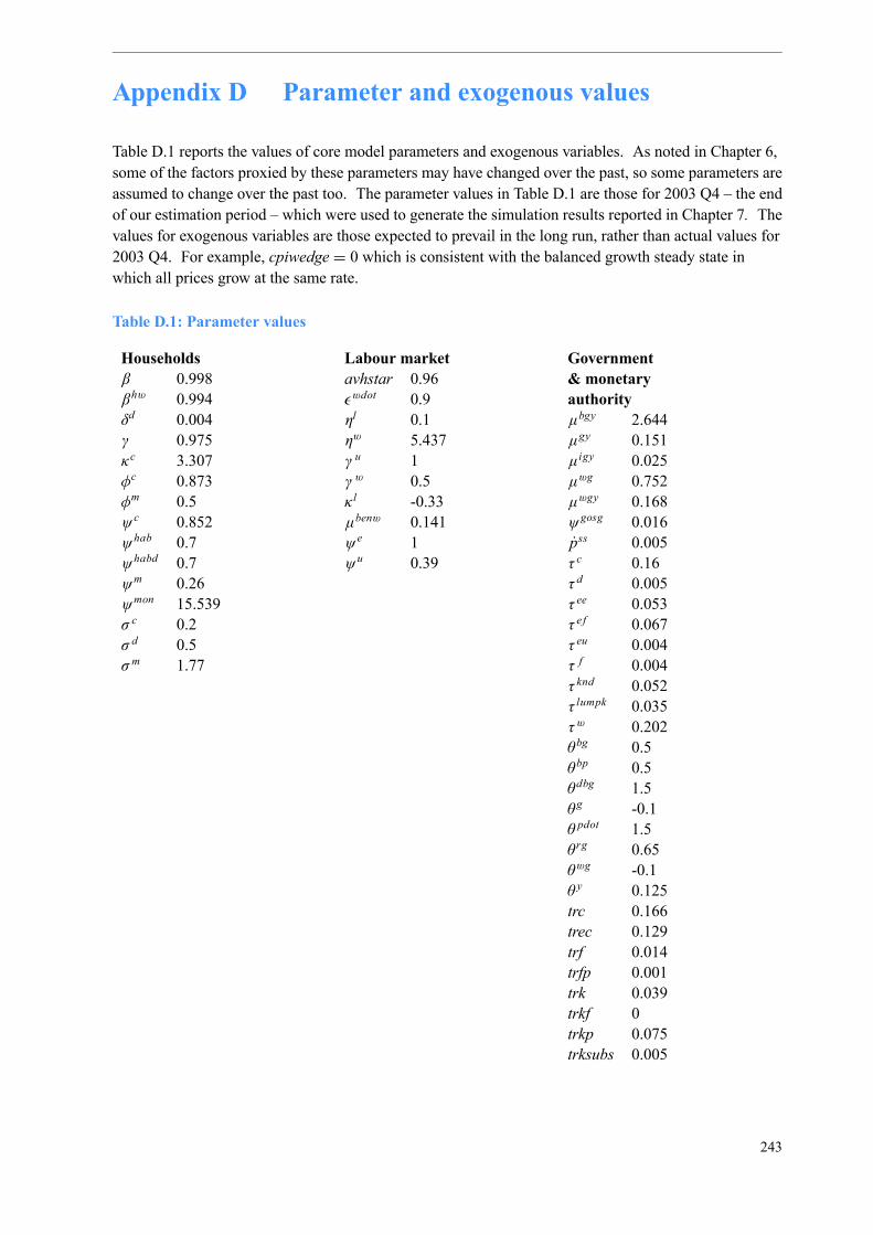
Appendix D Parameter and exogenous values
Table D.1 reports the values of core model parameters and exogenous variables. As noted in Chapter 6,some of the factors proxied by these parameters may have changed over the past, so some parameters areassumed to change over the past too. The parameter values in Table D.1 are those for 2003 Q4 – the endof our estimation period – which were used to generate the simulation results reported in Chapter 7. Thevalues for exogenous variables are those expected to prevail in the long run, rather than actual values for2003 Q4. For example, cpiwedge = 0 which is consistent with the balanced growth steady state inwhich all prices grow at the same rate.
Table D.1: Parameter values
Householdsβ 0.998βhw 0.994δd 0.004γ 0.975κc 3.307φc 0.873φm 0.5ψc 0.852ψhab 0.7ψhabd 0.7ψm 0.26ψmon 15.539σ c 0.2σ d 0.5σm 1.77
Labour marketavhstar 0.96wdot 0.9ηl 0.1ηw 5.437γ u 1γ w 0.5κ l -0.33µbenw 0.141ψe 1ψu 0.39
Government& monetaryauthorityµbgy 2.644µgy 0.151µigy 0.025µwg 0.752µwgy 0.168ψgosg 0.016pss 0.005τ c 0.16τ d 0.005τ ee 0.053τ e f 0.067τ eu 0.004τ f 0.004τ knd 0.052τ lumpk 0.035τw 0.202θbg 0.5θbp 0.5θdbg 1.5θ g -0.1θ pdot 1.5θ rg 0.65θwg -0.1θ y 0.125trc 0.166trec 0.129trf 0.014trfp 0.001trk 0.039trkf 0trkp 0.075trksubs 0.005
243
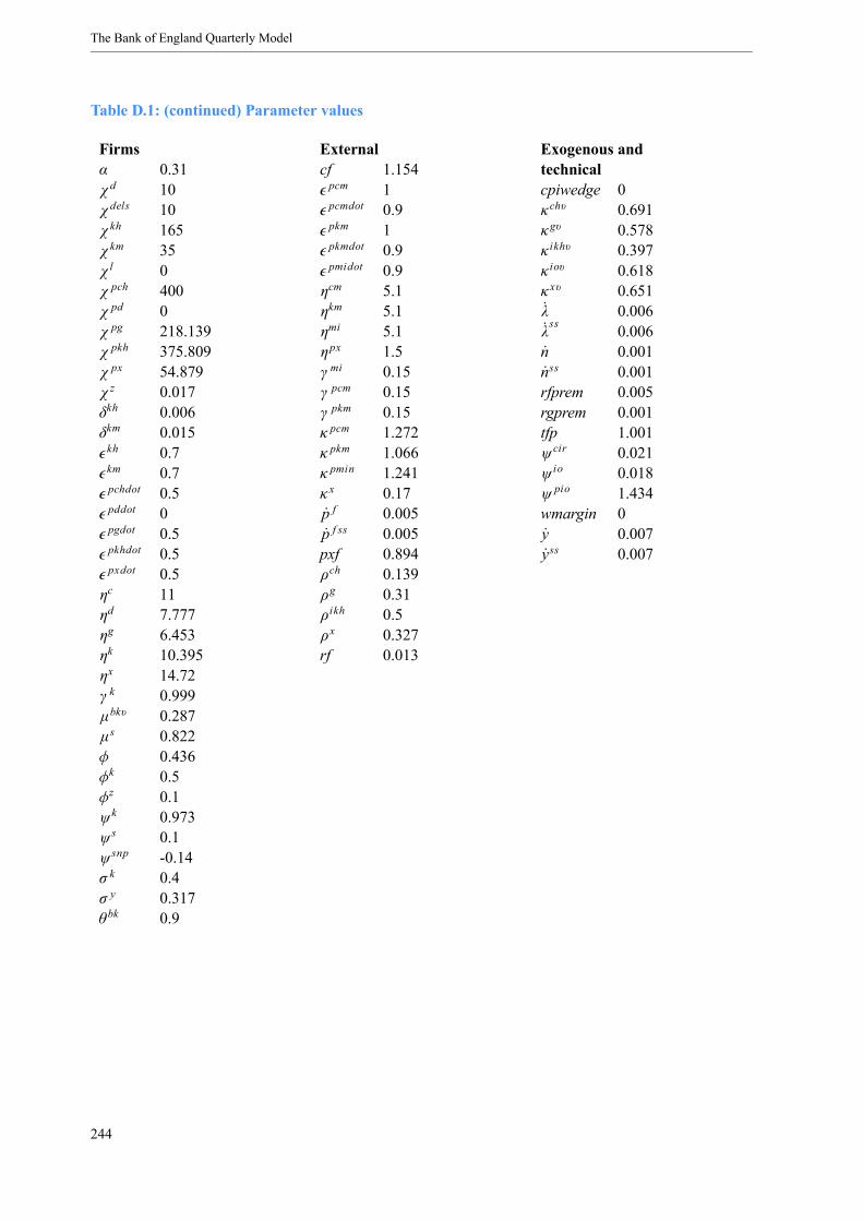
The Bank of England Quarterly Model
Table D.1: (continued) Parameter values
Firmsα 0.31χd 10χdels 10χ kh 165χ km 35χ l 0χ pch 400χ pd 0χ pg 218.139χ pkh 375.809χ px 54.879χ z 0.017δkh 0.006δkm 0.015kh 0.7km 0.7pchdot 0.5pddot 0pgdot 0.5pkhdot 0.5pxdot 0.5ηc 11ηd 7.777ηg 6.453ηk 10.395ηx 14.72γ k 0.999µbkv 0.287µs 0.822φ 0.436φk 0.5φz 0.1ψk 0.973ψ s 0.1ψ snp -0.14σ k 0.4σ y 0.317θbk 0.9
Externalcf 1.154pcm 1pcmdot 0.9pkm 1pkmdot 0.9pmidot 0.9ηcm 5.1ηkm 5.1ηmi 5.1ηpx 1.5γ mi 0.15γ pcm 0.15γ pkm 0.15κ pcm 1.272κ pkm 1.066κ pmin 1.241κ x 0.17p f 0.005p f ss 0.005pxf 0.894ρch 0.139ρg 0.31ρikh 0.5ρx 0.327rf 0.013
Exogenous andtechnicalcpiwedge 0κchv 0.691κgv 0.578κ ikhv 0.397κ iov 0.618κ xv 0.651λ 0.006λss 0.006n 0.001nss 0.001rfprem 0.005rgprem 0.001tfp 1.001ψcir 0.021ψ io 0.018ψ pio 1.434wmargin 0y 0.007yss 0.007
244