THE BABY BOOM, THE BABY BUST, AND THE HOUSING MARKET N. Gregory MANKIW … · 2013-02-05 · 238 N.G. Mankiw and D.N. Weil, Baby boom, baby bust, housing market 1950 1960 1970 1980

Regional Science and Urban Economics 19 (1989) 235-258. North-Holland

THE BABY BOOM, THE BABY BUST, AND THE HOUSING MARKET

N. Gregory MANKIW and David N. WEIL*

Harvard University, Cambridge, MA 02138, USA

Received August 1988, final version received January 1989

This paper examines the impact of major demographic changes on the housing market in the United States. The entry of the Baby Boom generation into its house-buying years is found to be the major cause of the increase in real housing prices in the 1970s. Since the Baby Bust generation is now entering its house-buying years, housing demand will grow more slowly in the 1990s than in any time in the past forty years. If the historical relation between housing demand and housing prices continues into the future, real housing prices will fall substantially over the next two decades.

1. Introduction

The dramatic rise in the number of births in the 1950s and the subsequent decline in the 1970s - the Baby Boom and the Baby Bust - are widely recognized as among the most important changes in the United States in the past 50 years. At the peak of the Baby Boom in 1957, 4.30 million babies were born in the United States. The year before the boom began, in 1945, 2.86 million babies were born, and at the trough of the Baby Bust in 1973, the figure was only 3.14 million. In this paper we examine how such major demographic changes affect the market for housing.

Our goals are both retrospective and prospective. We want to assess what impact these major demographic changes have had on the demand for housing and, further, how these changes in demand have affected residential investment and the price of housing. In addition, we want to assess what more recent demographic patterns imply about the housing market over the next twenty years.

Our analysis of both cross-sectional and time-series data leads us to three conclusions. First, large demographic changes of the sort we have observed induce large (and mostly predictable) changes in the demand for housing.

*We wish to thank David Cutler, Doug Elmendorf, Robert Gordon, Lawrence Katz, James Poterba, and Robert Shiller for helpful comments and Karen Dynan for research assistance.

016&0462/89/$3.50 0 1989, Elsevier Science Publishers B.V. (North-Holland)

236 N.G. Mankiw and D.N. Weil, Baby boom, baby bust, housing market

Second, these fluctuations in demand appear to have substantial impact on the price of housing. Third, recent demographic patterns imply that housing demand will grow more slowly over the next twenty years than in any time since World War II.

These findings have important implications for the public policy debate over housing. Between 1970 and 1980 housing prices rose dramatically: depending on the index, the real price of housing rose between 19 and 32 percent. This development generated many calls for government intervention to help provide more ‘affordable’ housing. Our results indicate that this increase in housing prices was largely attributable to the aging of the Baby Boom. Over the next twenty years, the Baby Bust generation will be in its house-buying years. As Kenneth Rosen (1984) has emphasized, this implies that housing demand will grow more slowly in the future. Our estimates suggest that real housing prices will fall substantially - indeed, real housing prices may well reach levels lower than those experienced at any time in the past forty years.

Our analysis proceeds as follows. We begin in section 2 by documenting the facts about the Baby Boom. We show the rise and subsequent decline in births and discuss the extent to which these demographic changes were predicted by contemporary observers.

In section 3 we examine the link between age and housing demand. Using cross-sectional data from the Census for years 1970 and 1980, we find that an individual generates little housing demand until age 20 - that is, children do not substantially increase a family’s quantity of housing. Housing demand rises sharply between ages 20 and 30, and remains approximately flat after age 30. This finding implies that an increase in the number of births has little immediate effect on the housing market, but generates an increase in housing demand twenty years hence.

We examine in section 4 how demographic changes in the United States have affected the demand for housing. We combine our cross-sectional results on age and housing demand with time series on the age composition of the population. We find that the Baby Boom of the 1950s led to rapid growth in housing demand in the 1970s and that the Baby Bust of the 1970s will lead to slow growth in housing demand in the 1990s.

In sections 5 and 6 we examine how housing demand affects the price of housing and the amount of residential investment. Section 5 is in the nature of an exploratory data analysis of the impact of changes in housing demand. We are unable to detect a statistically significant relation between demographic housing demand and the quantity of residential capital. Residential investment is such a ‘noisy’ time series that the standard errors we obtain are very large. There is, however, a significant relation between housing demand and the price of housing: a one percent increase in housing demand leads to a five percent increase in the real price of housing. We use this estimated

N.G. Mankiw and D.N. Weil, Baby boom, baby bust, housing market 237

YEAR

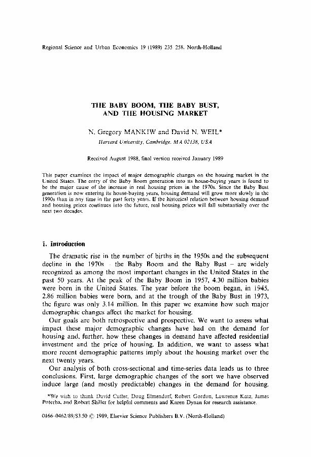
Fig. 1. Live births in the United States 191Ck1983.

relationship to examine how the slow growth in demand over the next twenty years will likely affect housing prices.

In section 6 we use an intertemporal model of the housing market, in the spirit of the one proposed by Poterba (1984) to examine the impact of changing housing demand. One implication of our findings is that the Baby Boom caused an increase in housing demand in the 1970s that was predictable far in advance. The model makes precise predictions about how such a forecastable increase in demand should affect the housing market. We examine what the model predicts and compare these predictions to experience. We conclude that the housing market probably should not be characterized as an efficient asset market in which prices reflect available information on future demand.

2. The facts about the Baby Boom

Fig. 1, which graphs the number of births over time, shows the Baby Boom very clearly. The low level of fertility during the Great Depression and the boom in births that lasted from 1946 to 1964 combine to produce a sharp step in the population structure. As this step aged, it had effects on the educational system, the labor market, the housing market, and the social security system.

One way to look at the magnitude of the Baby Boom is to look at the number of people at a given age. In 1960, 24.0 million people, or 13.3 percent of the population, were between ages 20 and 30; in 1980 the corresponding number was 44.6 million, or 19.7 percent of the population. Since this is the age in which people are forming new households and increasing their demand for housing, it is clear that the boom should have had a large effect on the housing market.


1950 1960 1970 1980 1990 2000 2010 2oJ20

YEAR

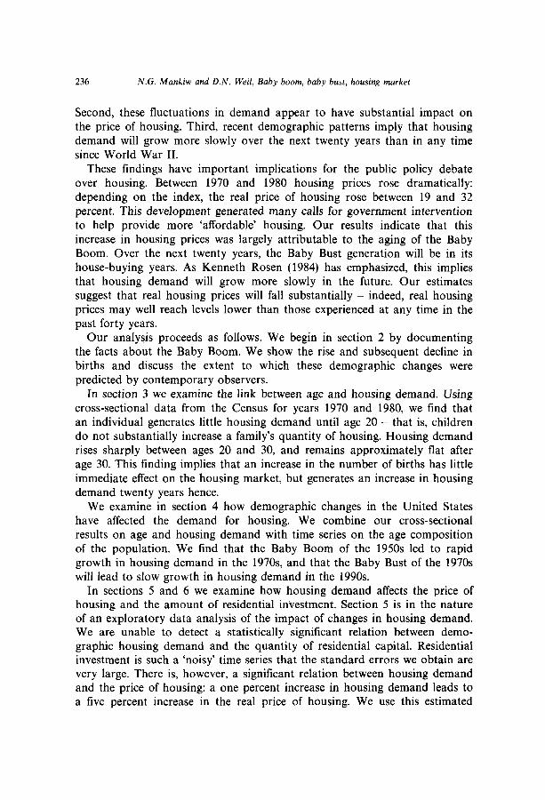
Fig. 2. Number of births: Actual and Census Bureau projections.

For our purposes, the exact cause of the Baby Boom is not important1 That the bulge in the population was significant and could be expected to move up through the age structure is clear enough that it does not need to be defended. Whether the boom was seen as being temporary or permanent is a tougher question to answer.

Fig. 2 presents the actual number of births per year from 1950 through 1983, and several contemporary forecasts made by the Census Bureau.* The lesson to be learned from looking at these forecasts is that forecasting births is a risky business. Any forecast of housing demand that depended sensitively on births would be highly suspect. Luckily, as we shall show below, forecasts of housing demand depend (as a first approximation) only on the population above the age of 20. Thus, housing demand can be forecast 20 years into the future before the unreliability of birth forecasts becomes a problem.3

3. Cross-sectional evidence on the demand for housing by age

We are interested in how housing demand is affected by changes in the

‘Russell (1982) notes that the boom was caused by increases in the number of women who married and the number of children per married woman, and the fact that married women tended to have children earlier. In terms of fertility, the boom can be seen in the number of births per 1,000 women aged 15 through 44, which jumped from a depression low of below 80 to a peak of above 120 around 1960, and fell to below 70 by 1980.

2The Census Bureau generally provides several forecasts for births, based on different assumptions about fertility. In cases where three forecasts were made, we took the middle one; in cases where four were made, we took the average of the middle two.

The series of actual births for the years before 1959 was subsequently adjusted upward to reflect underregistration. The result is that census forecasts are well below the actual number of births (even over short horizons for which birth forecasts should be highly accurate). We therefore adjust forecasts made before 1959 by a constant multiple computed by assuming that the first year of any forecast was correct.

)The 1983 forecast has been more accurate than most of its predecessors, at least so far. Actual births in 1987 were 3,829,000, compared to a forecast of 3,879,OOO.


size of different age cohorts. We begin our examination of this issue by using cross-sectional data to determine the link between age and the quantity of housing demanded.

Looking across individuals, the quantity of housing demanded is a function of age, income, and a variety of other household characteristics. Yet here we use data on only the first of these attributes: age. Our ultimate goal is to construct a variable on the aggregate demand for housing given information only on the age composition of the population. We are therefore not interested in the value of the true coefhcient on age in a multiple regression, Instead, we are interested in the best predictor of a household’s quantity of housing given information only on the age of its members. Any correlation of age with income and other household characteristics does not pose a problem - indeed, multicollinearity may be a strength, for it acts to eliminate any worry over the role of omitted variables.

We model demand for housing by a household as an additive function of the demand for housing of its members:

D= t Dj, j=l

where Dj is the demand of the jth member and N is the total number of people in the household. To the extent that there are economies of scale in the provision of housing services, this would not be the best way to estimate the housing demand of a given household. Yet if we are interested in predicting the housing demand of an entire population, and if the extent of household formation is fairly constant, then our approach should be accurate.4

The demand for housing of each individual is taken to be a function of age. We allow each age to have its own housing demand parameter, so that an individual’s demand is given by

where DUMMYO= 1 if age = 0, DVMM Yl = 1 if age = 1, etc. The parameter Cli tells us the quantity of housing demanded by a person of age i.

Combining (1) and (2) gives the equation for household demand:

D=a,~DUMMYOj+crl~DUMMYlj+-~+u.,g~DUMMY99j, (3)

4Hendershott (1987) studies the effects of changes in the propensity to form households on the demand for housing. We do not deny that such effects are important, but our primary interest is in changes in demand that are forecastable; we do not think that such changes are nearly as forecastable as changes in the age structure of the population.

240 N.G. Mankiw and D.N. Weir, Baby boom, baby bust, housing market

16-

14 -

I2 -

IO -

0-

6-

4-

-2 I I I I I I I I _ 0 20 40 60 80

AGE

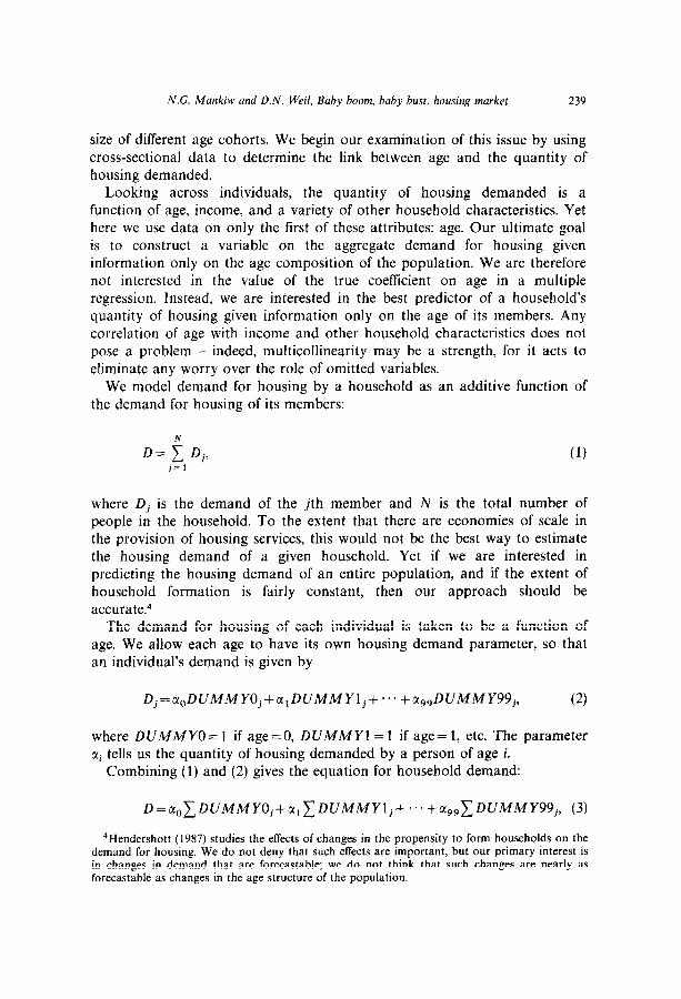
Fig. 3. Estimated housing demand by age.

We estimated (3) on a l-in-l,000 sample of the 1970 Census. The sample consists of 203,190 individuals grouped into 74,565 households. The left-hand side variable is the value of the property for the unit in which the household resides. For owner-occupied units this is reported directly. In the case of rental units, we used the approximation that the value is equal to 100 times the gross monthly rent.’ Leaving out units for which neither of these figures was available, our sample consisted of 53,518 households.

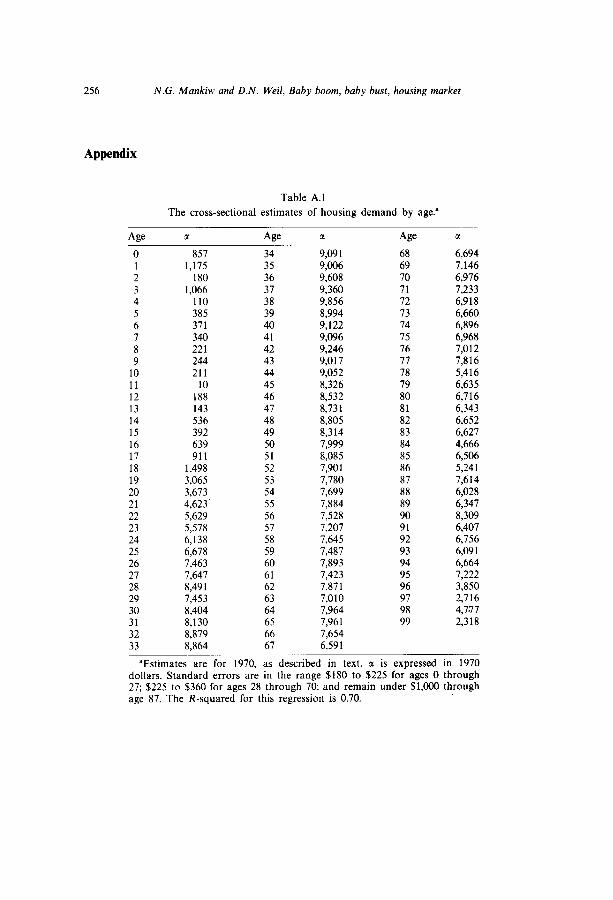
The solid line in Fig. 3 plots the estimated a’s, while the estimates themselves are in table A.1 in the appendix. Since the sample is so large, the standard errors are extremely small (less than $300 for all of the estimates below age 64). The dotted line in fig. 3 plots the LX’S for the same regression run on a sample from the 1980 Census, deflated into 1970 dollars by the GNP deflator.

The primary feature of the estimates is a sharp jump in the demand for housing between the ages of 20 and 30. As mentioned earlier, people below the age of 20 have little impact on the demand for housing. The result is qualitatively the same for 1970 and 1980 data. In the work below we use only the estimates from 1970.

A second feature of the results for both 1970 and 1980 is that the quantity of housing demanded appears to decline after age 40 by about one percent per year. This decline is probably attributable to the fact that, because of productivity growth, older cohorts have lower lifetime income than younger cohorts and therefore demand less housing.

A third feature of lig. 3 is the large shift upward between 1970 and 1980. The real value of housing for an adult of any given age increased almost 50 percent over this decade. Part of this increase is attributable to productivity growth: real disposable personal income per capita rose 22 percent from 1970

STo test the robustness of this approximation, we ran eq. (3) leaving out rental units and also with the value/rent ratio set to 80, 90, 110, and 120. The results were quite similar to our baseline case.


to 1980. But much of the rise in house value must be attributable to the 20

to 30 percent increase in the real price of housing. As long as the price elasticity of housing demand is less than one, an increase in the price of housing will increase the value of housing. The large increase in age-specific house value between 1970 and 1980 thus suggests that housing demand is fairly inelastic.

4. Shifts in housing demand due to the Baby Boom

Here we examine how changes in the age composition of the population affect the demand for housing over time. Our approach is to assume that the age structure of housing demand (that is, the set of tl’s estimated in the last section) is constant over time. We can then see how the age structure of housing demand interacts with shifts in the age structure of the population.657

More precisely, to obtain a measure that we interpret as the shift in housing demand due to demographics, we multiply the age structure of the population by the coefficients estimated in eq. (3) and sum for all cohorts. That is, if N(i,t) is the number of people of age i in year t, then housing demand in year t is

D, = c c$N(i, t).

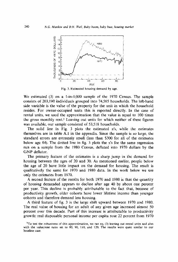
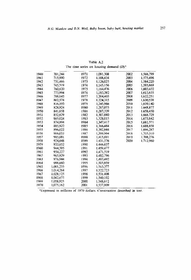
We use the U’S from the 1970 cross-sectional demand for housing. This time series on housing demand, which is measured in millions of 1970 dollars, is presented in table A.2 in the appendix. The growth rate of housing demand is plotted in fig. 4. For comparison, we also present in fig. 4 the growth in

housing demand computed with the 1980 a’s. The arrival of the Baby Boom in the housing market appears clearly as a

swelling in the rate of growth of demand that peaks around 1980. The rate of increase in housing demand from 1940 to 1950 was 1.84 percent per year; from 1950 to 1960, 1.16 percent; from 1960 to 1970, 1.31 percent; and from 1970 to 1980, 1.66 percent. Our forecast is that the rate of growth from 1980 to 1990 will be 1.33 percent per year; from 1990 to 2000, 0.68 percent, and from 2000 to 2010, 0.57 percent.

It is instructive to compare our estimate of the growth in housing demand with simpler demographic variables. Since our cross-sectional estimates indicate a large increase in housing demand from age 20 to 30 and

6To obtain the age structure of the population on an annual basis we combined data on births with estimates of mortality. Actual births are used through 1983, and the Census Bureau median forecast thereafter.

‘Our technique is similar to that employed by Hickman (1974); in place of our estimated a’s he uses age-specific rates of household headship.


YEAR - usmg coeff~cu?nts from the 1970 census

---- using coefficlenta from the i980 census

Fig. 4. Growth rate of housing demand.

YEAR

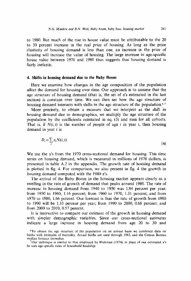
Fig. 5. Housing demand growth rate: Actual and projected.

Note: Each series is marked with a date indicating the year of the birth forecast on which it is based. For example, the series marked 1973 uses actual births through 1973 and the forecast of future births made in that year.

approximate constancy thereafter, our time series on housing demand is not very different from a time series on the adult population. The correlation between the growth in the population over 21 and the growth in our housing demand variable is 0.86. Our estimate of housing demand is, however, very different from the population including children. The correlation between the growth in the total population and the growth in our housing demand variable is -0.57. Hence, although our housing demand variable is quite similar to the adult population, it is not at all approximated by the total population.


Fig. 5 shows the forecasts of change in demand that would have been made using Census birth projections starting at various points in the postwar period. Despite the fact that birth projections were not very accurate, in every case forecasted demand growth tracks actual demand growth quite well for twenty years after the forecast is made. Because of the low demand for housing of children, forecasts of total housing demand made in the 1960s would have correctly predicted the increase in the rate of growth of housing demand in the 1970s.

5. From housing demand to prices and quantities

In the last section we combined the cross-sectional results on age and the quantity of housing demanded with time-series data on the age-composition of the population to generate a new time series on housing demand. This time series shows that the Baby Boom profoundly affected the demand for housing in the 1970s and that the Baby Bust will have the opposite impact on the housing market over the next twenty years. Our goal now is to examine the link between housing demand as measured by this time series and developments in the housing market.

We take two approaches to examining how these fluctuations in housing demand affect the housing market. Our first approach, which is pursued in this section, is statistical and relatively atheoretical: we examine how our time series on housing demand correlates with data on the housing market. Our second approach, which is pursued in the next section, is more theoretically correct but is relatively data-free: we calibrate a variant of Poterba’s model of the housing market and examine how, according to that model, large and predictable shifts in housing demand should affect the housing market. We also examine the extent to which available evidence is consistent with the model.

The reason we call the statistical analysis of this section relatively atheoretical is that any good theory of the housing market must take into account many subtle intertemporal issues. At any point in time, the stock of housing depends on past flows of investment; the flow of investment depends on the price of housing; the price of housing depends on current and expected future rents; the rent depends on the stock and the state of housing demand. While the model of the next section incorporates all these feed- backs, here we ignore them. The goal of the exploratory data analysis of this section is to see what stylized facts emerge.

5.1. Quantities

We begin by looking at whether there is any correlation between our housing demand variables and the quantity of housing. We measure the


Table 1

Housing demand and the housing stock.”

Dependent variable: log(stock); sample period: 1947-1985.

constant

time

log (demand)

log (gnp)

cost of funds

8.01 (7.81)

0.0095 (0.0366)

0.010 (0.652)

rho 0.971 (0.035)

R2 0.9996

DW 1.28

see 0.00704

“Standard errors are in parentheses.

5.14 (6.35)

- 0.0006 (0.0419)

0.173 (0.547)

0.149 (0.036)

0.976 0.976 (0.031) (0.034)

0.9997 0.9997

1.13 1.13

0.00581 0.00590

4.99 (7.28)

-0.0006 (0.0436)

0.182 (0.574)

0.149 (0.037)

- 0.00003 (0.00073)

-

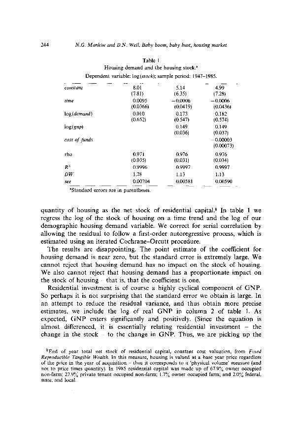
quantity of housing as the net stock of residential capital.* In table 1 we regress the log of the stock of housing on a time trend and the log of our demographic housing demand variable. We correct for serial correlation by allowing the residual to follow a first-order autoregressive process, which is estimated using an iterated Cochrane-Orcutt procedure.

The results are disappointing. The point estimate of the coefficient for housing demand is near zero, but the standard error is extremely large. We cannot reject that housing demand has no impact on the stock of housing. We also cannot reject that housing demand has a proportionate impact on the stock of housing - that is, that the coefficient is one.

Residential investment is of course a highly cyclical component of GNP. So perhaps it is not surprising that the standard error we obtain is large. In an attempt to reduce the residual variance, and thus obtain more precise estimates, we include the log of real GNP in column 2 of table 1. As expected, GNP enters significantly and positively. (Since the equation is almost differenced, it is essentially relating residential investment - the change in the stock - to the change in GNP. Thus, we are picking up the

8End of year total net stock of residential capital, constant cost valuation, from Fixed Reproducible Tangible Wealth. In this measure, housing is valued at a base year price regardless of the price in the year of acquisition - thus it corresponds to a ‘physical volume’ measure (and not to price times quantity). In 1985 residential capital was made up of 67.9% owner occupied non-farm; 27.9% private tenant occupied non-farm; 1.7% owner occupied farm; and 2.0% federal, state. and local.

N.G. Mankiw and D.N. Weir, Baby boom, baby bust, housing market 245

YEAR

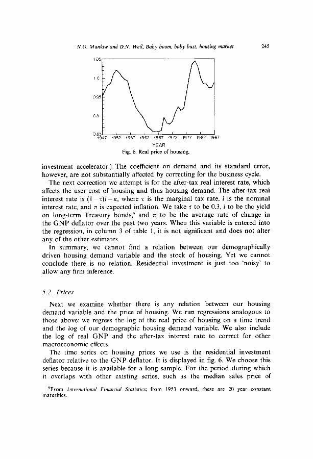
Fig. 6. Real price of housing.

investment accelerator.) The coefficient on demand and its standard error, however, are not substantially affected by correcting for the business cycle.

The next correction we attempt is for the after-tax real interest rate, which affects the user cost of housing and thus housing demand. The after-tax real interest rate is (1 -z)i-rr, where z is the marginal tax rate, i is the nominal interest rate, and rt is expected inflation. We take r to be 0.3, i to be the yield on long-term Treasury bonds9 and rc to be the average rate of change in the GNP deflator over the past two years. When this variable is entered into the regression, in column 3 of table 1, it is not significant and does not alter any of the other estimates.

In summary, we cannot find a relation between our demographically driven housing demand variable and the stock of housing. Yet we cannot conclude there is no relation. allow any firm inference.

Residential investment is just too ‘noisy’ to

5.2. Prices

Next we examine whether there is any relation between our housing demand variable and the price of housing. We run regressions analogous to those above: we regress the log of the real price of housing on a time trend and the log of our demographic housing demand variable. We also include the log of real GNP and the after-tax interest rate to correct for other macroeconomic effects.

The time series on housing prices we use is the residential investment deflator relative to the GNP deflator. It is displayed in fig. 6. We choose this series because it is available for a long sample. For the period during which it overlaps with other existing series, such as the median sales price of

9From International Financial Statistics; from 1953 onward, these are 20 year constant maturities.


constant

time

log (demand)

log (gnp)

cost of funds

-63.1 (9.2)

- 0.065 (0.010)

4.65 (0.68)

- 73.4 (7.9)

-0.081 (0.009)

5.29 (0.56)

0.234 (0.097)

-0.0035 (0.0021)

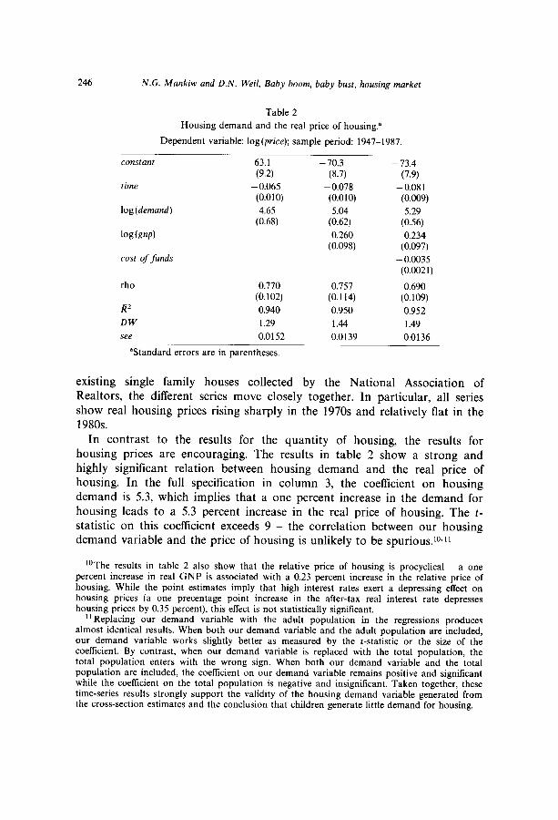
Table 2

Housing demand and the real price of housing.”

Dependent variable: log(price); sample period: 1947-1987.

- 70.3

(8.7) - 0.078

(0.010)

5.04 (0.62)

0.260 (0.098)

rho 0.770 0.757 0.690 (0.102) (0.114) (0.109)

R2 0.940 0.950 0.952

DW 1.29 1.44 1.49

see 0.0152 0.0139 0.0136

“Standard errors are in parentheses.

existing single family houses collected by the National Association of Realtors, the different series move closely together. In particular, all series show real housing prices rising sharply in the 1970s and relatively flat in the 1980s.

In contrast to the results for the quantity of housing, the results for housing prices are encouraging. The results in table 2 show a strong and highly significant relation between housing demand and the real price of housing. In the full specification in column 3, the coefficient on housing demand is 5.3, which implies that a one percent increase in the demand for housing leads to a 5.3 percent increase in the real price of housing. The t- statistic on this coefficient exceeds 9 - the correlation between our housing demand variable and the price of housing is unlikely to be spurious.lO*ll

toThe results in table 2 also show that the relative price of housing is procyclical - a one percent increase in real GNP is associated with a 0.23 percent increase in the relative price of housing. While the point estimates imply that high interest rates exert a depressing effect on housing prices (a one precentage point increase in the after-tax real interest rate depresses housing prices by 0.35 percent), this effect is not statistically signiticant.

“Replacing our demand variable with the adult population in the regressions produces almost identical results. When both our demand variable and the adult oooulation are included. our demand variable works slightly better as measured by the t-statistfic or the size of the coefftcient. By contrast, when our demand variable is replaced with the total population, the total population enters with the wrong sign. When both our demand variable and the total population are included, the coefficient on our demand variable remains positive and signiticant while the coefficient on the total population is negative and insignificant. Taken together, these time-series results strongly support the validity of the housing demand variable generated from the cross-section estimates and the conclusion that children generate little demand for housing.


Y 4- 9

-2.4 a

s - - I

z 2 - ‘\,, -2,o k$

- z

% ‘\ ‘\

‘\ ‘\ -1.6 w

5 o- \

_M I

‘1 s

2 - /

\_I’ ‘\ -is2 Q

‘\

5 -2- 6

f

0.8 +

8

5 _4- Change I” Price

>L 5

Change an Demand - 0.4 L&

a I I I I I I 0 2

1940 1950 1960 i970 1980 1990 2000

YEAR

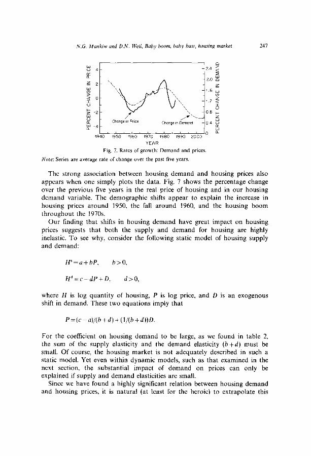
Fig. 7. Rates of growth: Demand and prices.

Note: Series are average rate of change over the past five years.

The strong association between housing demand and housing prices also appears when one simply plots the data. Fig. 7 shows the percentage change over the previous five years in the real price of housing and in our housing demand variable. The demographic shifts appear to explain the increase in housing prices around 1950, the fall around 1960, and the housing boom throughout the 1970s.

Our finding that shifts in housing demand have great impact on housing prices suggests that both the supply and demand for housing are highly inelastic. To see why, consider the following static model of housing supply and demand:

H”=a+bP, b > 0,

Hd=c-dP+D, d > 0,

where H is log quantity of housing, shift in demand. These two equations

P is log price, and D is an exogenous imply that

P=(c-a)/(b+d)+(l/(b+d))D.

For the coefficient on housing demand to be large, as we found in table 2, the sum of the supply elasticity and the demand elasticity (b +d) must be small. Of course, the housing market is not adequately described in such a static model. Yet even within dynamic models, such as that examined in the next section, the substantial impact of demand on prices can only be explained if supply and demand elasticities are small.

Since we have found a highly significant relation between housing demand and housing prices, it is natural (at least for the heroic) to extrapolate this


relation forward to see what it implies for future housing prices. As we have emphasized earlier, the changes in housing demand caused by changes in birth rates are forecastable far in advance. Therefore, we can be confident about our predictions regarding future housing demand.

The implication for future housing prices is perhaps apparent from fig. 7, which graphs the percentage increase in housing prices and the percentage increase in housing demand. It shows that housing demand will grow more slowly over the next twenty years than at any time in our sample. If the historical relation between demand and prices continues to hold, it appears that the real price of housing will fall about 3 percent a year. More formal forecasting using the regressions yields the same answer. The regression in the first column of table 2 implies that real housing prices will fall by a total of 47 percent by the year 2007. Thus, according to this forecasting equation, the housing boom of the past twenty years will more than reverse itself in the next twenty.

At this point we should interject a note of caution about this forecast. Every good student of econometrics can recite the perils of forecasting beyond the experience of the data. The predicted growth of our housing demand variable is lower than has been experienced over the past forty years, and the period of low growth is protracted. Hence, we cannot be confident about precisely what effects this slow growth will have. Yet experience does tell us that slow growth in demand is associated with falling prices. Even if the fall in housing prices is only one-half what our equation predicts, it will likely be one of the major economic events of the next two decades.

6. Housing demand in an intertemporal model

We now turn to examining the impact of changing demand in an intertemporal model of the housing market. The model that we use is a slight variation on that of Poterba (1984). In contrast to Poterba, we ignore issues of taxation and of the effect of inflation on the cost of owning a home, and concentrate on the effects of changes in demand attributable to demographic changes.i2

6.1. The elements of the model

Let H be the stock of housing. We assume that the flow of housing services is proportional to the stock of housing. The demand for housing is given by the equation

lZThe model we examine is partial equilibrium in nature. For a general equilibrium treatment of some of these issues, see Manchester (1988).


Hd=f(R)N, f’>O,

where R is the real rental price and N is the adult population. N is a shift variable which is meant to capture the effect of demographic changes of the type discussed in section 4. The market-clearing rent is thus given by

R = R(h), R’<O,

where h = H/N is housing per adult, and R( .) is the inverse of f( .). We let P represent the real price of a standardized unit of housing. (We

ignore any distinction between land and structures.) For simplicity we assume that the operating cost of owning a home is some constant, r, times the value of the house. This constant is meant to incorporate the opportunity cost of capital, property taxes, maintenance, and depreciation. The arbitrage condition for the path of housing prices is

R(h)=rP-P. (5)

This equation says that the rent must equal the user cost, which equals the operating costs minus the capital gain. This implies

P=rP- R(h). (6)

This equation tells us how the price of housing evolves over time. Gross investment in housing is taken to be an increasing function of the

price of housing and proportional to the scale of the economy as measured by the adult population:

E~+~H=$(P)N, *bo,

where 6 is the rate of depreciation. Let n be the rate of growth of the population - that is, n = N/N. We can rewrite this equation terms of h rather than H. Differentiating H/N with respect to time and substituting gives

h = fiJN - n( H/N)

=$(P)-(n+d)h. (7)

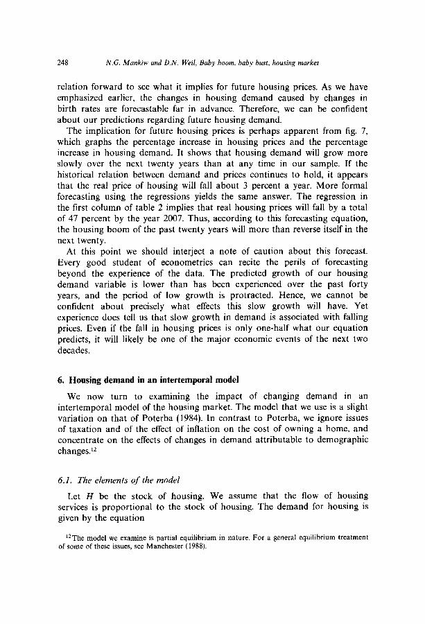
Population growth, n, thus enters as a shift variable in the model. Fig. 8 combines eqs. (6) and (7) to give the familiar phase plane

representation of the housing market. In steady state, the state variable h and the costate variable P are constant. The arrows show the implied dynamics


h Fig. 8. The model’s dynamics.

of the economy when it is out of steady state. For any given value of h, P jumps to the stable arm and the economy converges to the steady state.

6.2. Simulating a Baby Boom

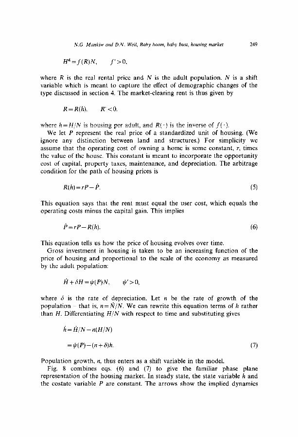
Now consider the effects of a hypothetical Baby Boom. The economy is in a steady state with growth at a rate of one percent per year. In hypothetical year 1960 it is announced that from years 1970 through 1979, the growth rate of the adult population will be two percent per year, after which it will return permanently to one percent. As can be seen in the phase diagram in fig. 9, the price of housing jumps up upon the announcement, rises until sometime in the middle of the high growth period, then gradually falls back

to its steady state level. To get a feel for the potential magnitude of the price changes, we simulate

the model under the assumption that the demand elasticity is l/2, the supply elasticity is 1, the operating cost r is 5 percent, and the depreciation rate 6 is

P

h

Fig. 9. A baby boom: An anticipated temporary increase in population growth.


1950 1960 1970 1980 1990 2000 2010 2020

YEAR _ ,,forward looktng model --- no~ve’ model

Fig. 10. Response of housing price to a theoretical baby boom.

2 percent. Although these supply and demand elasticities are somewhat smaller than is generally accepted, we choose them to generate large price responses. Rosen (1979) estimates that the elasticity of demand is about 1.13 Poterba (1984) estimates that the supply elasticity is between 0.5 and 2, while Topel and Rosen (1988) estimate that the supply elasticity is about 3. After studying our base case, we will consider the price responses generated by these alternative parameters.

The solid line in fig. 10 plots the simulated path of prices. We see that upon the announcement of the Baby Boom, the price of housing jumps about three percent. From 1960 to 1970, the price rises about 3 percent more in anticipation of the increased demand. The price rises an additional one percent from 1970 to 1975, and then gradually falls back to the original level. Thus, the price changes generated by the model under perfect foresight are not very large, and almost all of the price rise takes place before the increased demand arrives.

In assessing this forward-looking model of the housing market, it is instructive to consider a simple alternative: suppose that market participants are ‘naive’ in the sense that, whatever the price of housing at a given time, they expect it to remain constant at that level. If this is the case, there are no expected capital gains, and the price of housing is determined simply by the rental market. That is.

P = R(h)/r.

13Rosen’s estimate, which is based on cross-sectional data, should probably be considered a long-run elasticity. Over short horizons, perhaps even as long as a decade, the demand elasticity is likely smaller. Moving costs play a key role here, since they make the demand elasticity zero for many people. One weakness of the intertemporal model used here is that it does not distinguish between long-run and short-run demand elasticities.


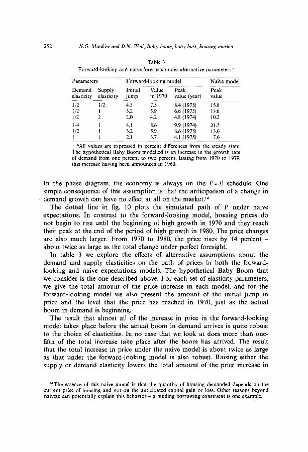
Table 3

Forward-looking and naive forecasts under alternative parameters.”

Parameters Forward-looking model Naive model

Demand Supply Initial Value Peak Peak elasticitv elasticitv iumo in 1970 value (vear) value

112 112 4.3 7.5 8.4 (1975) 15.8 l/2 1 3.2 5.9 6.6 (1975) 13.6 l/2 2 2.0 4.2 4.8 (1974) 10.2

l/4 1 4.1 8.6 9.9 (1974) 21.5 l/2 1 3.2 5.9 6.6 (1975) 13.6 1 1 2.1 3.7 4.1 (1975) 7.6

“All values are expressed in percent differences from the steady state. The hypothetical Baby Boom modelled is an increase in the growth rate of demand from one percent to two percent, lasting from 1970 to 1979, this increase having been announced in 1960.

In the phase diagram, the economy is always on the P=O schedule. One simple consequence of this assumption is that the anticipation of a change in demand growth can have no effect at all on the market.14

The dotted line in fig. 10 plots the simulated path of P under naive expectations. In contrast to the forward-looking model, housing prices do not begin to rise until the beginning of high growth in 1970 and they reach their peak at the end of the period of high growth in 1980. The price changes are also much larger. From 1970 to 1980, the price rises by 14 percent - about twice as large as the total change under perfect foresight.

In table 3 we explore the effects of alternative assumptions about the demand and supply elasticities on the path of prices in both the forward- looking and naive expectations models. The hypothetical Baby Boom that we consider is the one described above. For each set of elasticity parameters, we give the total amount of the price increase in each model, and for the forward-looking model we also present the amount of the initial jump in price and the level that the price has reached in 1970, just as the actual boom in demand is beginning.

The result that almost all of the increase in price in the forward-looking model takes place before the actual boom in demand arrives is quite robust to the choice of elasticities. In no case that we look at does more than one- fifth of the total increase take place after the boom has arrived. The result that the total increase in price under the naive model is about twice as large as that under the forward-looking model is also robust. Raising either the supply or demand elasticity lowers the total amount of the price increase in

t4The essence of this naive model is that the quantity of housing demanded depends on the current price of housing and not on the anticipated capital gain or loss. Other reasons beyond naivete can potentially explain this behavior - a binding borrowing constraint is one example.


either model. In general, alternative assumptions about the supply and demand elasticities do not change the qualitative properties of either model. Setting these elasticities as high as suggested by some of the literature discussed above, however, does reduce the size of the price increase in both models, but especially in the forward-looking model, to near insignificance.

6.3. Does the model fit experience?

While we do not formally test the forward-looking model of the housing market, there are several reasons to think that it cannot come close to fitting the data. First, consider the timing of the run-up in prices in the 1970s. Both housing prices and our housing demand series rose swiftly in this decade. But the increase in demand growth could have been perfectly predicted ten years in advance. In a forward-looking model, most of the increase in prices should have taken place before the increase in demand actually arrived.

Similarly, the forward-looking model does not properly capture the timing of the turn-around in prices. An examination of fig. 7 shows that housing prices peaked at almost exactly the time that the demand growth began declining. The forward-looking model implies that prices should turn down before demand growth. The model with naive expectations described at the end of the last section, by contrast, does have the property that prices turn down at the same time as demand.

Second, consider the magnitude of the price increase. The arbitrage condition in the forward-looking model makes it difficult for prices to rise very quickly in the absence of news. The forward-looking model reacts to our simulated ‘Baby Boom’ with a price increase of seven percent - far from the 20 to 30 percent rise observed from 1970 to 1980. Again the model with naive expectations comes closer to matching the facts: the total rise in prices in response to a simulated Baby Boom in this model is much greater than in the forward-looking model, and it takes place over a shorter period of time.

As a means of salvaging the forward-looking model, one might argue that the rise in prices in the 1970s was due not to the anticipated demand increases in that decade but to the gradual arrival of ‘news’ about future demand growth. Fig. 5 shows, however, that considering the arrival of news only makes the forward-looking model look worse. The positive news about demand in our sample period arrived during the 195Os, when it became clear that the forecasts of births made in the early 1950s were too low. During the 1970s by contrast, the news that arrived was negative: the low birth rates of the decade showed that earlier forecasts were too high. News about births in the 1970s should have made housing prices fall.

6.4. Is the housing market an efficient asset market?

Our simulation of the intertemporal model suggests that naive expec-

RS.UE D


tations better characterizes the housing market than does perfect foresight. In other words, the fluctuations in prices caused by fluctuations in demand do not appear to be foreseen by the market, even though these fluctuations in demand were foreseeable (at least in principle). Thus, the arbitrage condition (6) appears not to characterize housing prices.

More direct tests also suggest that the housing market cannot be viewed as an efficient asset market in which prices fully reflect available information and returns are unforecastable. We can test the proposition that real housing prices follow a random walk by regressing the change in the log of housing prices on the change in the log of our demographic demand variable. We obtain, with standard errors in parentheses,

A log P = -0.06 + 4.74 log D, (0.02) (1.1)

N=40, D.W=1.36, R2=0.30, s.e.e.=0.016.

Remember that this housing demand variable, which forecasts 30 percent of real capital gains in housing, is known about 20 years in advance. Thus, housing prices are not all a random walk.

The failure of the random walk hypothesis for housing prices, however, need not imply the failure of (6) and the existence of profit opportunities. If the rent-price ratio moves in the opposite direction from the expected capital gain, then the total return (rent and capital gain together) could be unforecastable. In fact, using the CPI’s component for rent, we find that the rent-price ratio is negatively related to next year’s capital gain:‘5

A log P = 0.03 - O.O24R/P, (0.02) (0.018)

N=40, D.W.=O.99, R2=0.02, s.e.e.=0.019.

Yet this statistical relation is very weak: the R2 is far smaller for the rent-price ratio than for the change in demand. When both regressors are included, we obtain

A log P = - 0.11 + 5.8A log D + O.O24R/P, (0.04) ( 1.4) (0.019)

t5Unfortunately, since we have only an index of rents, we cannot compute the total return on housing and examine directly whether it is related to our demand variable. This also implies that the coeflicient on R/P cannot be easily interpreted. We should note that Apgar (1987) has argued that the CPI for rent is a bad measure because of changes in the quality of the rental units over time.


N=40, D.II!=1.41, R2=0.32, s.e.e.=0.016.

The change in demand remains significant, while the rent-price ratio has the wrong sign. In contrast to what an efficient market would require, the rent- price ratio is not the best predictor of the capital gain. It is possible, of course, that if we had better data on rents, we would find the evidence more favorable to the efficient markets hypothesis. Based on the available evidence, however, it seems that the housing market should not be viewed as an efficient asset market.16

7. Conclusion

We have documented that changes in the number of births over time lead to large and predictable changes in the demand for housing. These changes in housing demand appear to have substantial impact on the price of housing. If the historical pattern continues over the next twenty years, housing prices will fall to levels lower than observed at any time in recent history.

Does our finding imply that readers of this paper should sell their homes and become renters? There are at least three reasons that such an action may not be called for. First, there continue to be substantial advantages to home ownership. Some of these advantages are attributable to the tax code and some are attributable to solving the principal-agent problem that exists between landlord and tenant. Second, there is substantial uncertainty about future housing prices. Not only are there unforeseeable macroeconomic developments, but individual regions of the country will experience housing booms or busts. The best way to hedge the uncertainty about future housing costs is to pay them in advance - that is, to be a homeowner. Third, most homeowners have unrealized capital gains (at least in nominal terms). Becoming a renter requires realizing these capital gains and paying tax at a current rate of 28 percent. For these three reasons, there is no easy way for the typical person to take advantage of advance knowledge of a fall in housing prices.

What effect will the fall in housing demand have on the economy as a whole? It is of course difficult to judge. Since it appears that current housing prices do not fully reflect low future demand, the United States may be currently overinvesting in residential capital. When such drop in demand does become apparent, it is conceivable that we will see a large and sudden drop in housing prices and residential investment, which may be a potential source of macroeconomic instability. Falling housing prices may also induce increases in saving, as individuals perceive their housing equity as insufficient to fund their retirement. The macroeconomic effects of falling housing demand appear to be a fruitful topic for future research.

16For further evidence on this question, see Case and Shiller (1988).


Appendix

Table A.1

The cross-sectional estimates of housing demand by age.”

Age

8 9

10 11 12 13 14 15 16 17 18 19 20 21 22 23 24 25 26 27 28 29 30 31 32 33

a

857 1,175

180 1.066 ‘110 385 371 340 221 244 211

10 188 143 536 392 639 911

1,498 3,065 3,673 4.623 51629 5,578 6.138 6;678 7,463 7.647 8,49 1 7.453 8.404 8,130 8,879 8,864

Age 34 35 36 37 38 39 40 41 42 43 44 45 46 47 48 49 50 51 52 53 54 55 56 57 58 59 60 61 62 63 64 65 66 67

a

9,091 9,006 9,608 9.360 9;856 8,994 9,122 9,096 9,246 9,017 9,052 8,326 8,532 8,73 1 8,805 8,314 7,999 8,085 7,901 7,780 7,699 7,884 7,528 7,207 7,645 7,487 7,893 7,423 7,871 7,010 7,964 7,961 7,654 6,591

Age a

68 6,694 69 7,146 70 6,976 71 7,233 72 6,918 73 6,660 74 6,896 75 6,968 76 7,012 77 7,816 78 5,416 79 6,635 80 6,716 81 6,343 82 6,652 83 6,627 84 4,666 85 6,506 86 5,241 87 7,614 88 6,028 89 6,347 90 8,309 91 6,407 92 6,756 93 6,09 1 94 6.664 95 7;222 96 3,850 97 2,716 98 4,777 99 2,318

“Estimates are for 1970, as described in text. a is expressed in 1970 dollars. Standard errors are in the range $180 to $225 for ages 0 through 27; $225 to $360 for ages 28 through 70; and remain under $1,000 through age 87. The R-squared for this regression is 0.70.


1940 1941 1942 1943 1944 1945 1946 1947 1948 1949 1950 1951 1952 1953 1954 1955 1956 1957 1958 1959 1960 1961 1962 1963 1964 1965 1966 1967 1968 1969 1970

Table A.2

The time series on housing demand (D).”

976,944

701,244 7 15,990

988.660

73 1,466 745,519 760,620 773,894 788,645 802,574 816,193 828,924 841,658 852,629 865,024 874,894 885,822 896,022 906,033 915,681 924,648 933,652 944,395 954,227 965,829

1,001,255 1.0143264 1,028,125 lJt42.675 1,058,925 1,075,162

1971 1972 1973 1974 1975 1976 1977 1978 1979 1980 1981

1994

1982 1983

1995

1984 1985 1986 1987 1988 1989 1990 1991 1992 1993

1996 1997 1998 1999 2000 2001

1,091,308 1,108,434 1,126,025 1,145,156 1.164.476 1;183;382 1,204,403 1,224,315 1,245,966 1,267,075 1,287,339 1,307,880 1,328,015 1,347,417 1,366,484 1,382,844 1,399,964 1,415,691 1,431,576 1446,637 1,459,477 1,471,519 1.482.796 1,493,492 1,503,859 1,513,377 1,522,723 1.531.408 1,540,102 1,548,612 1,557,809

2002 2003 2004 2005 2006 2007 2008 2009 2010 2011 2012 2013 2014 2015 2016 2017 2018 2019 2020

1,566,799 1,575,496 1,584,220 1,593,669 1603,432 1,613,635 1,622,251 1,630,538 1,639,140 1648,877 1.658.450 (666,729 1,673,842 1,681,571 1,688,858 1,696,287 1,703,310 1,708,276 1,712,960

“Expressed in millions of 1970 dollars. Construction described in text.


References

Apgar, William C., Jr., 1987, Recent trends in real rents, Working paper W87-5 (Joint Center for Housing Studies of MIT and Harvard, Cambridge, MA).

Bureau of the Census, various years, Current population reports, Series P-25: Projections of the population of the United States by age, sex, and race, Various issues.

Case, Karl E. and Robert J. Shiller, 1988, The efficiency of the market for single family homes, American Economic Review 79.

Hickman, Bert, 1974, What became of the building cycle?, in: Paul David and Melvin Reder, eds., Nations and households in economic growth: Essays in honor of Moses Abramovitz (Academic Press, New York) 291-314.

Manchester, Joyce, 1988, The baby boom, housing, and loanable funds, Canadian Journal of Economics, forthcoming.

Poterba, James M., 1984, Tax subsidies to owner-occupied housing: An asset market approach, Quarterly Journal of Economics 99, 729-752.

Rosen, Harvey, 1979, Housing decisions and the US. income tax, Journal of Public Economics 11, l-23.

Rosen, Kenneth, 1984, Affordable housing: New policies and the housing and mortgage markets (Balhnger, Cambridge).

Russell, Louise B., 1982, The baby boom generation and the economy (Brookings Institution, Washington, DC).

Topel, Robert and Sherwin Rosen, 1988, Housing investment in the United States, Journal of Political Economy 96, 7 18-740.

US. Department of Commerce, Bureau of Economic Analysis, 1987, Fixed reproducible tangible wealth in the United States, 192585 (US. Government Printing Office, Washington, DC).

Documents

THE BABY BOOM, THE BABY BUST, AND THE HOUSING MARKET N. Gregory MANKIW … · 2013-02-05 · 238 N.G. Mankiw and D.N. Weil, Baby boom, baby bust, housing market 1950 1960 1970 1980