The Asynchronous Bounded-Cycle model

Theoretical Computer Science 412 (2011) 5580–5601

Contents lists available at SciVerse ScienceDirect

Theoretical Computer Science

journal homepage: www.elsevier.com/locate/tcs

The Asynchronous Bounded-Cycle model

Peter Robinson ∗, Ulrich SchmidTechnische Universität Wien, Embedded Computing Systems Group (E182/2), Treitlstrasse 1-3, A-1040 Vienna, Austria

a r t i c l e i n f o

Keywords:Fault-tolerant distributed algorithmsPartially synchronous modelsClock synchronizationVLSI

a b s t r a c t

This paper shows how synchrony conditions can be added to the purely asynchronousmodel in a way that avoids any reference to message delays and computing step times,as well as system-wide constraints on execution patterns and network topology. OurAsynchronous Bounded-Cycle (ABC)model just bounds the ratio of the number of forward-and backward-oriented messages in certain (‘‘relevant’’) cycles in the space–time diagramof an asynchronous execution. We show that clock synchronization and lock-step roundscan be implemented and proved correct in the ABC model, even in the presence ofByzantine failures. Furthermore, we prove that any algorithm working correctly in thepartially synchronousΘ-Model alsoworks correctly in the ABCmodel. In our proof, we firstapply a novel method for assigning certain message delays to asynchronous executions,which is based on a variant of Farkas’ theorem of linear inequalities and a non-standardcycle space of graphs. Using methods from point-set topology, we then prove that theexistence of this delay assignment implies model indistinguishability for time-free safetyand liveness properties. We also introduce several weaker variants of the ABC model,and relate our model to the existing partially synchronous system models, in particular,the classic models of Dwork, Lynch and Stockmayer and the query–response model byMostefaoui, Mourgaya, and Raynal. Finally, we discuss some aspects of the ABC model’sapplicability in real systems, in particular, in the context of VLSI Systems-on-Chip.

© 2010 Elsevier B.V. All rights reserved.

1. Introduction

Adding synchrony conditions, relating the occurrence times of certain events in a distributed system to each other, is the‘‘classic’’ approach for circumventing impossibility results as (Fischer et al. [23]) in fault-tolerant distributed computing. Thefollowing models in between synchrony and asynchrony, which are all sufficiently strong for solving the pivotal consensusproblem, have been proposed in the literature:

(1) The Archimedeanmodel by Vitányi [38] bounds the ratio betweenmaximumend-to-end delays andminimal computingstep times.

(2) The classic partially synchronousmodels byDwork et al. [17], Chandra and Toueg [11] and the semi-synchronousmodelsof Ponzio and Strong [36], Attiya et al. [7] boundmessage delays as well as the ratio of minimal andmaximal computingstep times.

(3) The MCM model by Fetzer [20] assumes that all the received messages are correctly classified as ‘‘slow’’ or ‘‘fast’’,depending on the message delays.

This research is supported by the Austrian Science Foundation (FWF) projects P17757 and P20529. A preliminary version of this paper (Robinson andSchmid (2008)) received the best paper award at SSS’08.∗ Corresponding author. Tel.: +43 158801 18253; fax: +43 158801 18297.

E-mail addresses: [email protected] (P. Robinson), [email protected] (U. Schmid).

0304-3975/$ – see front matter© 2010 Elsevier B.V. All rights reserved.doi:10.1016/j.tcs.2010.08.001

http://dx.doi.org/10.1016/j.tcs.2010.08.001

http://www.elsevier.com/locate/tcs

http://www.elsevier.com/locate/tcs

mailto:[email protected]

mailto:[email protected]

http://dx.doi.org/10.1016/j.tcs.2010.08.001

P. Robinson, U. Schmid / Theoretical Computer Science 412 (2011) 5580–5601 5581

(4) TheΘ-Model by Le Lann and Schmid [29], Widder et al. [41] andWidder and Schmid [40] bounds the ratio between themaximal and minimal end-to-end delay of messages simultaneously in transit.

(5) The FAR Model by Fetzer et al. [22] assumes lower bounded computing step times and message delays with finiteaverage.

(6) The Weak Timely Link (WTL) models of Aguilera et al. [4], Malkhi et al. [30] and Hutle et al. [26] assume that onlymessages sent via certain links have bounded end-to-end delay.

(7) TheMMRmodel byMostefaoui et al. [35] suggested for implementing failure detectors in systemswith process crashes,which assumes certain order properties for round-trip responses.

All these models, except (3) and (7), refer to individual message delays and/or computing step times, and most of theminvolve explicit time bounds and constraints that must hold within the entire system.

This paper shows how to add synchrony assumptions – sufficiently strong for implementing lock-step rounds, and hencefor solving many important distributed computing problems – to the asynchronous model in a way that

(1) entirely avoids any reference to message delays and computing step times, and(2) does not require system-wide constraints on potential computing step and communication patterns and network

topology.

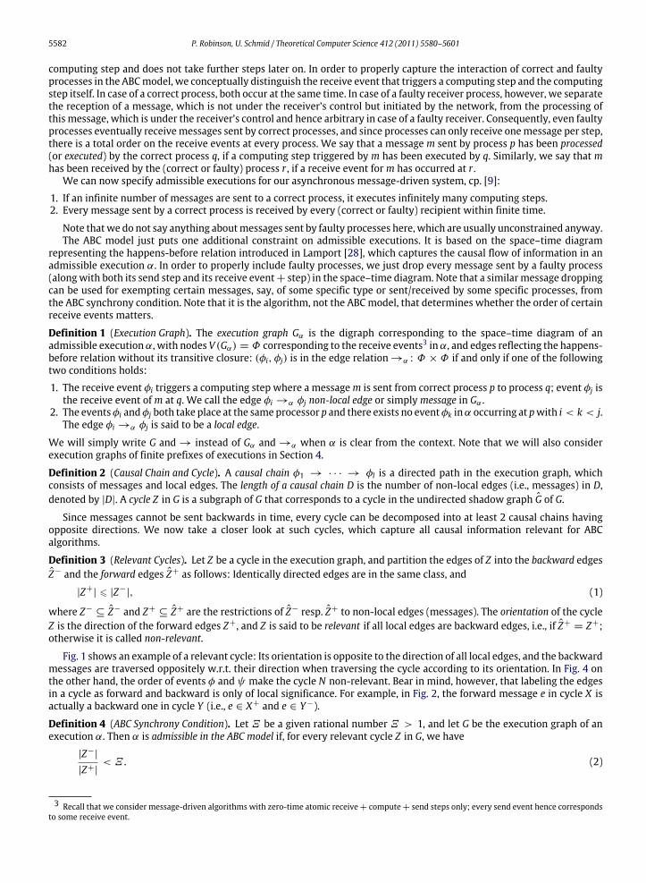
More specifically, our Asynchronous Bounded-Cycle (ABC) model bounds the ratio of the number of forward and backwardmessages in certain ‘‘relevant’’ cycles in the space–time diagram of an asynchronous execution only. Intuitively speaking,there is only one scenario that is admissible in the purely asynchronous model but not in the ABC model: A chain C1 of k1consecutive messages, starting at process q and ending at p, that properly ‘‘spans’’ (i.e., covers w.r.t. real time; see Fig. 1)another causal chain C2 from q to p involving k2 ⩾ k1Ξ messages, for some model parameterΞ > 1.

Consequently, individualmessage delays can be arbitrary, ranging from 0 to any finite value; theymay even continuouslyincrease. There is no relation at all between computing step times and/or message delays at processes that do not exchangemessages; this also includes purely one-way communication (‘‘isolated chains’’). For processes that do exchange messages,message delays and step times in non-relevant cycles and isolated chains can also be arbitrary. Only cumulative delays ofchains C1 and C2 in relevant cycles must yield the event order as shown in Fig. 1. That is, the sum of the message delaysalong C2 must not become so small that C1 could span k1Ξ or more messages in C2. Note carefully that this is not just astatic system-wide condition that is imposed by the system model, but also depends on the message pattern created byan algorithm. Nevertheless, ABC algorithms can exploit it for ‘‘timing out’’ relevant message chains, and hence for failuredetection.

Besides introducing the ABC model in Section 2, our paper provides the following contributions:

• In Section 3, we provide and prove correct a simple Byzantine fault-tolerant clock synchronization algorithm and a lock-step round simulation for the ABC model.• In Section 4, we prove that all message-driven algorithms designed and proved correct for the Θ-Model also work

correctly in the ABC model, despite the fact that most ABC executions are not admissible in the Θ-Model. In the quiteinvolved proofs, we use methods from linear algebra and point-set topology, some of which may also be applicable inother contexts as well.• In Section 5, we relate the ABC model to the existing partially synchronous models, and show that it is strictly weaker in

terms of synchrony.We also provide a short discussion of some practical aspects, in the context of VLSI systems-on-chip.• In Section 6we introduce someweaker variants of theABCmodel, including unknownand/or eventualmodel parameters.

Some conclusions and directions of further research in Section 7 eventually complete our paper.

2. The ABC model

We consider a system of n distributed processes, connected by a (not necessarily fully connected) point-to-point networkwith finite but unboundedmessage delays.We neither assume FIFO communication channels nor an authentication service,but we do assume that processes know the sender of a received message.

Every process executes an instance of a distributed algorithm and is modeled as a state machine. Its local executionconsists of a sequence of atomic, zero-time computing steps, each involving the reception of exactly one1 message, a statetransition, and the sending of zero or more messages to a subset of the processes in the system. Since the ABC model isentirely time-free, i.e., does not introduce any time-related bounds, we restrict our attention to message-driven algorithms,cp. [8,9,31]: Computing steps at process p are exclusively triggered by a single incoming message at p, with an external‘‘wake-up message’’ initiating p’s very first computing step; we assume that this very first step occurs before any messagefrom another process is received.

Among the n processes, at most f may be Byzantine faulty. A faulty process may deviate arbitrarily from the behavior ofcorrect processes as described above2; it may of course just crash as well, in which case it possibly fails to complete some

1 An algorithm cannot learn anything from receiving multiple asynchronous messages at the same time, cp. [16].2 More specifically, we do not assume that Byzantine processes or messages sent by such processes adhere to any synchrony requirements.

5582 P. Robinson, U. Schmid / Theoretical Computer Science 412 (2011) 5580–5601

computing step and does not take further steps later on. In order to properly capture the interaction of correct and faultyprocesses in the ABCmodel, we conceptually distinguish the receive event that triggers a computing step and the computingstep itself. In case of a correct process, both occur at the same time. In case of a faulty receiver process, however, we separatethe reception of a message, which is not under the receiver’s control but initiated by the network, from the processing ofthis message, which is under the receiver’s control and hence arbitrary in case of a faulty receiver. Consequently, even faultyprocesses eventually receivemessages sent by correct processes, and since processes can only receive onemessage per step,there is a total order on the receive events at every process. We say that a message m sent by process p has been processed(or executed) by the correct process q, if a computing step triggered by m has been executed by q. Similarly, we say that mhas been received by the (correct or faulty) process r , if a receive event form has occurred at r .

We can now specify admissible executions for our asynchronous message-driven system, cp. [9]:

1. If an infinite number of messages are sent to a correct process, it executes infinitely many computing steps.2. Every message sent by a correct process is received by every (correct or faulty) recipient within finite time.

Note thatwe do not say anything aboutmessages sent by faulty processes here, which are usually unconstrained anyway.The ABC model just puts one additional constraint on admissible executions. It is based on the space–time diagram

representing the happens-before relation introduced in Lamport [28], which captures the causal flow of information in anadmissible execution α. In order to properly include faulty processes, we just drop every message sent by a faulty process(alongwith both its send step and its receive event+ step) in the space–time diagram. Note that a similarmessage droppingcan be used for exempting certain messages, say, of some specific type or sent/received by some specific processes, fromthe ABC synchrony condition. Note that it is the algorithm, not the ABCmodel, that determines whether the order of certainreceive events matters.

Definition 1 (Execution Graph). The execution graph Gα is the digraph corresponding to the space–time diagram of anadmissible execution α, with nodes V (Gα) = Φ corresponding to the receive events3 in α, and edges reflecting the happens-before relation without its transitive closure: (φi, φj) is in the edge relation→α : Φ × Φ if and only if one of the followingtwo conditions holds:

1. The receive event φi triggers a computing step where a messagem is sent from correct process p to process q; event φj isthe receive event ofm at q. We call the edge φi →α φj non-local edge or simplymessage in Gα .

2. The eventsφi andφj both take place at the sameprocessor p and there exists no eventφk inα occurring at pwith i < k < j.The edge φi →α φj is said to be a local edge.

We will simply write G and→ instead of Gα and→α when α is clear from the context. Note that we will also considerexecution graphs of finite prefixes of executions in Section 4.

Definition 2 (Causal Chain and Cycle). A causal chain φ1 → · · · → φl is a directed path in the execution graph, whichconsists of messages and local edges. The length of a causal chain D is the number of non-local edges (i.e., messages) in D,denoted by |D|. A cycle Z in G is a subgraph of G that corresponds to a cycle in the undirected shadow graph G of G.

Since messages cannot be sent backwards in time, every cycle can be decomposed into at least 2 causal chains havingopposite directions. We now take a closer look at such cycles, which capture all causal information relevant for ABCalgorithms.

Definition 3 (Relevant Cycles). Let Z be a cycle in the execution graph, and partition the edges of Z into the backward edgesZ− and the forward edges Z+ as follows: Identically directed edges are in the same class, and

|Z+| ⩽ |Z−|, (1)

where Z− ⊆ Z− and Z+ ⊆ Z+ are the restrictions of Z− resp. Z+ to non-local edges (messages). The orientation of the cycleZ is the direction of the forward edges Z+, and Z is said to be relevant if all local edges are backward edges, i.e., if Z+ = Z+;otherwise it is called non-relevant.

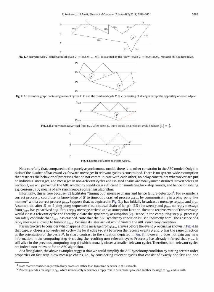
Fig. 1 shows an example of a relevant cycle: Its orientation is opposite to the direction of all local edges, and the backwardmessages are traversed oppositely w.r.t. their direction when traversing the cycle according to its orientation. In Fig. 4 onthe other hand, the order of events φ and ψ make the cycle N non-relevant. Bear in mind, however, that labeling the edgesin a cycle as forward and backward is only of local significance. For example, in Fig. 2, the forward message e in cycle X isactually a backward one in cycle Y (i.e., e ∈ X+ and e ∈ Y−).

Definition 4 (ABC Synchrony Condition). Let Ξ be a given rational number Ξ > 1, and let G be the execution graph of anexecution α. Then α is admissible in the ABC model if, for every relevant cycle Z in G, we have

|Z−||Z+|

< Ξ . (2)

3 Recall that we consider message-driven algorithms with zero-time atomic receive+ compute+ send steps only; every send event hence correspondsto some receive event.


Fig. 1. A relevant cycle Z , where a causal chain C2 = m1l1m2 . . .m5l2 is spanned by the ‘‘slow’’ chain C1 = m6m7m8m9 . Messagem3 has zero delay.

Fig. 2. An execution graph containing relevant cycles X , Y , and the combined cycle X ⊕ Y , consisting of all edges except the oppositely oriented edge e.

slow

fast

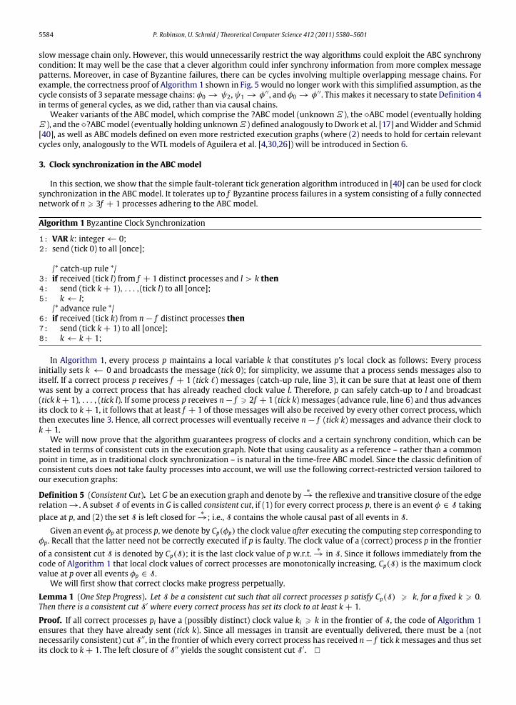
Fig. 3. If a reply message arrived from pslow after event ψ , there would be a relevant cycle Z where |Z−|

|Z+ | =42 .

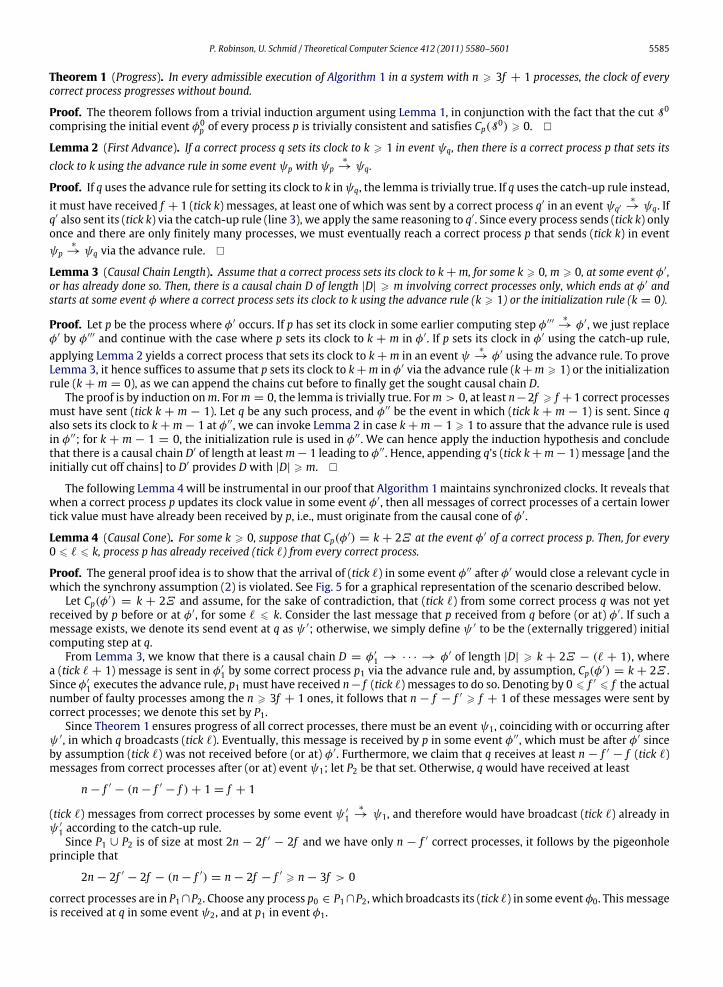
Fig. 4. Example of a non-relevant cycle N .

Note carefully that, compared to the purely asynchronous model, there is no other constraint in the ABCmodel: Only theratio of the number of backward vs. forwardmessages in relevant cycles is constrained. There is no system-wide assumptionthat restricts the behavior of processes that do not communicate with each other, no delay constraints whatsoever are puton individual messages, and messages in non-relevant cycles and isolated chains are totally unconstrained. Nevertheless, inSection 3, wewill prove that the ABC synchrony condition is sufficient for simulating lock-step rounds, and hence for solvinge.g. consensus by means of any synchronous consensus algorithm.

Informally, this is true because (2) facilitates ‘‘timing out’’ message chains and hence failure detection4: For example, acorrect process p could use its knowledge of Ξ to timeout a crashed process pslow, by communicating in a ping-pong-likemanner5 with a correct process pfast. Suppose that, as depicted in Fig. 3, p has initially broadcast a message to pslow and pfast.Assume that, after Ξ = 2 ping-pong sequences (i.e., a causal chain of length 2Ξ ) between p and pfast, no reply messagefrom pslow has yet arrived at p. If this replymessage arrived at p at some point later on, then the receive event of this messagewould close a relevant cycle and thereby violate the synchrony assumption (2). Hence, in the computing step ψ , process pcan safely conclude that pslow has crashed. Note that the ABC synchrony condition is used indirectly here: The absence of areply message allows p to timeout pslow, because its later arrival would violate the ABC synchrony condition.

It is instructive to considerwhat happens if themessage from pslow arrives before the eventψ occurs, as shown in Fig. 4. Inthat case, ψ closes a non-relevant cycle—the local edge (φ, ψ) between the receive events φ and ψ has the same directionas the orientation of the cycle N . In sharp contrast to the situation depicted in Fig. 3, however, p does not gain any newinformation in the computing step ψ closing the resulting non-relevant cycle: Process p has already inferred that pslow isstill alive in the previous computing step φ (which actually closes a smaller relevant cycle). Therefore, non-relevant cyclesare indeed non-relevant for an ABC algorithm.

At a first glance, the above examples suggest that we could simplify the ABC synchrony condition by stating certain orderproperties on fast resp. slow message chains, i.e., by considering relevant cycles that consist of exactly one fast and one

4 Note that we consider only crash-faulty processes rather than Byzantine behavior in this example.5 Process p sends a message to pfast which immediately sends back a reply. This in turn causes p to send another message to pfast and so forth.


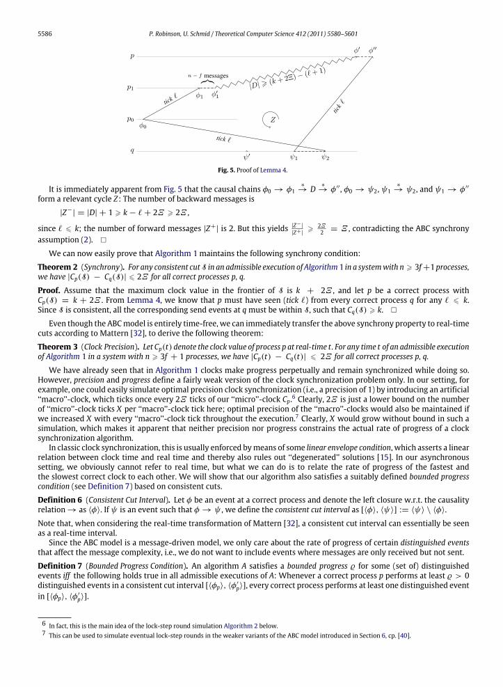
slow message chain only. However, this would unnecessarily restrict the way algorithms could exploit the ABC synchronycondition: It may well be the case that a clever algorithm could infer synchrony information from more complex messagepatterns. Moreover, in case of Byzantine failures, there can be cycles involving multiple overlapping message chains. Forexample, the correctness proof of Algorithm 1 shown in Fig. 5 would no longer work with this simplified assumption, as thecycle consists of 3 separatemessage chains: φ0 → ψ2,ψ1 → φ′′, and φ0 → φ′′. This makes it necessary to state Definition 4in terms of general cycles, as we did, rather than via causal chains.

Weaker variants of the ABC model, which comprise the ?ABC model (unknownΞ ), the ABC model (eventually holdingΞ ), and the ?ABCmodel (eventually holding unknownΞ ) defined analogously to Dwork et al. [17] andWidder and Schmid[40], as well as ABC models defined on even more restricted execution graphs (where (2) needs to hold for certain relevantcycles only, analogously to the WTL models of Aguilera et al. [4,30,26]) will be introduced in Section 6.

3. Clock synchronization in the ABC model

In this section, we show that the simple fault-tolerant tick generation algorithm introduced in [40] can be used for clocksynchronization in the ABC model. It tolerates up to f Byzantine process failures in a system consisting of a fully connectednetwork of n ⩾ 3f + 1 processes adhering to the ABC model.

Algorithm 1 Byzantine Clock Synchronization

1: VAR k: integer← 0;2: send (tick 0) to all [once];

/* catch-up rule */3: if received (tick l) from f + 1 distinct processes and l > k then4: send (tick k+ 1), . . . ,(tick l) to all [once];5: k← l;

/* advance rule */6: if received (tick k) from n− f distinct processes then7: send (tick k+ 1) to all [once];8: k← k+ 1;

In Algorithm 1, every process p maintains a local variable k that constitutes p’s local clock as follows: Every processinitially sets k ← 0 and broadcasts the message (tick 0); for simplicity, we assume that a process sends messages also toitself. If a correct process p receives f + 1 (tick ℓ) messages (catch-up rule, line 3), it can be sure that at least one of themwas sent by a correct process that has already reached clock value l. Therefore, p can safely catch-up to l and broadcast(tick k+ 1), . . . , (tick l). If some process p receives n− f ⩾ 2f + 1 (tick k) messages (advance rule, line 6) and thus advancesits clock to k+ 1, it follows that at least f + 1 of those messages will also be received by every other correct process, whichthen executes line 3. Hence, all correct processes will eventually receive n− f (tick k) messages and advance their clock tok+ 1.

We will now prove that the algorithm guarantees progress of clocks and a certain synchrony condition, which can bestated in terms of consistent cuts in the execution graph. Note that using causality as a reference – rather than a commonpoint in time, as in traditional clock synchronization – is natural in the time-free ABC model. Since the classic definition ofconsistent cuts does not take faulty processes into account, we will use the following correct-restricted version tailored toour execution graphs:

Definition 5 (Consistent Cut). Let G be an execution graph and denote by∗→ the reflexive and transitive closure of the edge

relation→. A subset S of events in G is called consistent cut, if (1) for every correct process p, there is an event φ ∈ S takingplace at p, and (2) the set S is left closed for

∗→; i.e., S contains the whole causal past of all events in S.

Given an event φp at process p, we denote by Cp(φp) the clock value after executing the computing step corresponding toφp. Recall that the latter need not be correctly executed if p is faulty. The clock value of a (correct) process p in the frontierof a consistent cut S is denoted by Cp(S); it is the last clock value of p w.r.t.

∗→ in S. Since it follows immediately from the

code of Algorithm 1 that local clock values of correct processes are monotonically increasing, Cp(S) is the maximum clockvalue at p over all events φp ∈ S.

We will first show that correct clocks make progress perpetually.Lemma 1 (One Step Progress). Let S be a consistent cut such that all correct processes p satisfy Cp(S) ⩾ k, for a fixed k ⩾ 0.Then there is a consistent cut S′ where every correct process has set its clock to at least k+ 1.Proof. If all correct processes pi have a (possibly distinct) clock value ki ⩾ k in the frontier of S, the code of Algorithm 1ensures that they have already sent (tick k). Since all messages in transit are eventually delivered, there must be a (notnecessarily consistent) cut S′′, in the frontier of which every correct process has received n− f tick kmessages and thus setits clock to k+ 1. The left closure of S′′ yields the sought consistent cut S′.


Theorem 1 (Progress). In every admissible execution of Algorithm 1 in a system with n ⩾ 3f + 1 processes, the clock of everycorrect process progresses without bound.

Proof. The theorem follows from a trivial induction argument using Lemma 1, in conjunction with the fact that the cut S0

comprising the initial event φ0p of every process p is trivially consistent and satisfies Cp(S

0) ⩾ 0.

Lemma 2 (First Advance). If a correct process q sets its clock to k ⩾ 1 in event ψq, then there is a correct process p that sets itsclock to k using the advance rule in some event ψp with ψp

∗→ ψq.

Proof. If q uses the advance rule for setting its clock to k inψq, the lemma is trivially true. If q uses the catch-up rule instead,it must have received f + 1 (tick k) messages, at least one of which was sent by a correct process q′ in an eventψq′

∗→ ψq. If

q′ also sent its (tick k) via the catch-up rule (line 3), we apply the same reasoning to q′. Since every process sends (tick k) onlyonce and there are only finitely many processes, we must eventually reach a correct process p that sends (tick k) in eventψp

∗→ ψq via the advance rule.

Lemma 3 (Causal Chain Length). Assume that a correct process sets its clock to k+m, for some k ⩾ 0, m ⩾ 0, at some event φ′,or has already done so. Then, there is a causal chain D of length |D| ⩾ m involving correct processes only, which ends at φ′ andstarts at some event φ where a correct process sets its clock to k using the advance rule (k ⩾ 1) or the initialization rule (k = 0).

Proof. Let p be the process where φ′ occurs. If p has set its clock in some earlier computing step φ′′′∗→ φ′, we just replace

φ′ by φ′′′ and continue with the case where p sets its clock to k + m in φ′. If p sets its clock in φ′ using the catch-up rule,applying Lemma 2 yields a correct process that sets its clock to k+m in an event ψ

∗→ φ′ using the advance rule. To prove

Lemma 3, it hence suffices to assume that p sets its clock to k+m in φ′ via the advance rule (k+m ⩾ 1) or the initializationrule (k+m = 0), as we can append the chains cut before to finally get the sought causal chain D.

The proof is by induction onm. Form = 0, the lemma is trivially true. Form > 0, at least n−2f ⩾ f +1 correct processesmust have sent (tick k + m − 1). Let q be any such process, and φ′′ be the event in which (tick k + m − 1) is sent. Since qalso sets its clock to k+m− 1 at φ′′, we can invoke Lemma 2 in case k+m− 1 ⩾ 1 to assure that the advance rule is usedin φ′′; for k + m − 1 = 0, the initialization rule is used in φ′′. We can hence apply the induction hypothesis and concludethat there is a causal chain D′ of length at leastm− 1 leading to φ′′. Hence, appending q’s (tick k+m− 1) message [and theinitially cut off chains] to D′ provides Dwith |D| ⩾ m.

The following Lemma 4 will be instrumental in our proof that Algorithm 1maintains synchronized clocks. It reveals thatwhen a correct process p updates its clock value in some event φ′, then all messages of correct processes of a certain lowertick value must have already been received by p, i.e., must originate from the causal cone of φ′.

Lemma 4 (Causal Cone). For some k ⩾ 0, suppose that Cp(φ′) = k + 2Ξ at the event φ′ of a correct process p. Then, for every

0 ⩽ ℓ ⩽ k, process p has already received (tick ℓ) from every correct process.

Proof. The general proof idea is to show that the arrival of (tick ℓ) in some event φ′′ after φ′ would close a relevant cycle inwhich the synchrony assumption (2) is violated. See Fig. 5 for a graphical representation of the scenario described below.

Let Cp(φ′) = k + 2Ξ and assume, for the sake of contradiction, that (tick ℓ) from some correct process q was not yet

received by p before or at φ′, for some ℓ ⩽ k. Consider the last message that p received from q before (or at) φ′. If such amessage exists, we denote its send event at q as ψ ′; otherwise, we simply define ψ ′ to be the (externally triggered) initialcomputing step at q.

From Lemma 3, we know that there is a causal chain D = φ′1 → · · · → φ′ of length |D| ⩾ k + 2Ξ − (ℓ + 1), wherea (tick ℓ + 1) message is sent in φ′1 by some correct process p1 via the advance rule and, by assumption, Cp(φ

′) = k + 2Ξ .Since φ′1 executes the advance rule, p1 must have received n− f (tick ℓ) messages to do so. Denoting by 0 ⩽ f ′ ⩽ f the actualnumber of faulty processes among the n ⩾ 3f + 1 ones, it follows that n − f − f ′ ⩾ f + 1 of these messages were sent bycorrect processes; we denote this set by P1.

Since Theorem 1 ensures progress of all correct processes, there must be an event ψ1, coinciding with or occurring afterψ ′, in which q broadcasts (tick ℓ). Eventually, this message is received by p in some event φ′′, which must be after φ′ sinceby assumption (tick ℓ) was not received before (or at) φ′. Furthermore, we claim that q receives at least n − f ′ − f (tick ℓ)messages from correct processes after (or at) event ψ1; let P2 be that set. Otherwise, qwould have received at least

n− f ′ − (n− f ′ − f )+ 1 = f + 1

(tick ℓ) messages from correct processes by some event ψ ′1∗→ ψ1, and therefore would have broadcast (tick ℓ) already in

ψ ′1 according to the catch-up rule.Since P1 ∪ P2 is of size at most 2n − 2f ′ − 2f and we have only n − f ′ correct processes, it follows by the pigeonhole

principle that

2n− 2f ′ − 2f − (n− f ′) = n− 2f − f ′ ⩾ n− 3f > 0

correct processes are in P1∩P2. Choose any process p0 ∈ P1∩P2, which broadcasts its (tick ℓ) in some event φ0. This messageis received at q in some event ψ2, and at p1 in event φ1.


messages

tick

tick

tick

Fig. 5. Proof of Lemma 4.

It is immediately apparent from Fig. 5 that the causal chains φ0 → φ1∗→ D

∗→ φ′′, φ0 → ψ2, ψ1

∗→ ψ2, and ψ1 → φ′′

form a relevant cycle Z: The number of backward messages is

|Z−| = |D| + 1 ⩾ k− ℓ+ 2Ξ ⩾ 2Ξ ,

since ℓ ⩽ k; the number of forward messages |Z+| is 2. But this yields |Z−|

|Z+| ⩾ 2Ξ2 = Ξ , contradicting the ABC synchrony

assumption (2).

We can now easily prove that Algorithm 1 maintains the following synchrony condition:

Theorem 2 (Synchrony). For any consistent cutS in an admissible execution of Algorithm1 in a systemwith n ⩾ 3f+1 processes,we have |Cp(S) − Cq(S)| ⩽ 2Ξ for all correct processes p, q.

Proof. Assume that the maximum clock value in the frontier of S is k + 2Ξ , and let p be a correct process withCp(S) = k + 2Ξ . From Lemma 4, we know that p must have seen (tick ℓ) from every correct process q for any ℓ ⩽ k.Since S is consistent, all the corresponding send events at qmust be within S, such that Cq(S) ⩾ k.

Even though the ABCmodel is entirely time-free, we can immediately transfer the above synchrony property to real-timecuts according to Mattern [32], to derive the following theorem:

Theorem 3 (Clock Precision). Let Cp(t) denote the clock value of process p at real-time t. For any time t of an admissible executionof Algorithm 1 in a system with n ⩾ 3f + 1 processes, we have |Cp(t) − Cq(t)| ⩽ 2Ξ for all correct processes p, q.

We have already seen that in Algorithm 1 clocks make progress perpetually and remain synchronized while doing so.However, precision and progress define a fairly weak version of the clock synchronization problem only. In our setting, forexample, one could easily simulate optimal precision clock synchronization (i.e., a precision of 1) by introducing an artificial‘‘macro’’-clock, which ticks once every 2Ξ ticks of our ‘‘micro’’-clock Cp.6 Clearly, 2Ξ is just a lower bound on the numberof ‘‘micro’’-clock ticks X per ‘‘macro’’-clock tick here; optimal precision of the ‘‘macro’’-clocks would also be maintained ifwe increased X with every ‘‘macro’’-clock tick throughout the execution.7 Clearly, X would grow without bound in such asimulation, which makes it apparent that neither precision nor progress constrains the actual rate of progress of a clocksynchronization algorithm.

In classic clock synchronization, this is usually enforced bymeans of some linear envelope condition, which asserts a linearrelation between clock time and real time and thereby also rules out ‘‘degenerated’’ solutions [15]. In our asynchronoussetting, we obviously cannot refer to real time, but what we can do is to relate the rate of progress of the fastest andthe slowest correct clock to each other. We will show that our algorithm also satisfies a suitably defined bounded progresscondition (see Definition 7) based on consistent cuts.

Definition 6 (Consistent Cut Interval). Let φ be an event at a correct process and denote the left closure w.r.t. the causalityrelation→ as ⟨φ⟩. If ψ is an event such that φ→ ψ , we define the consistent cut interval as [⟨φ⟩, ⟨ψ⟩] := ⟨ψ⟩ \ ⟨φ⟩.

Note that, when considering the real-time transformation of Mattern [32], a consistent cut interval can essentially be seenas a real-time interval.

Since the ABC model is a message-driven model, we only care about the rate of progress of certain distinguished eventsthat affect the message complexity, i.e., we do not want to include events where messages are only received but not sent.

Definition 7 (Bounded Progress Condition). An algorithm A satisfies a bounded progress ϱ for some (set of) distinguishedevents iff the following holds true in all admissible executions of A: Whenever a correct process p performs at least ϱ > 0distinguished events in a consistent cut interval [⟨φp⟩, ⟨φ

′p⟩], every correct process performs at least one distinguished event

in [⟨φp⟩, ⟨φ′p⟩].

6 In fact, this is the main idea of the lock-step round simulation Algorithm 2 below.7 This can be used to simulate eventual lock-step rounds in the weaker variants of the ABC model introduced in Section 6, cp. [40].


Theorem 4. Algorithm1 satisfies the bounded progressϱ = 4Ξ+1 for the distinguished event that represents clock incrementingand message broadcasting (=send to all).

Proof. From the code of Algorithm 1, it is apparent that incrementing the clock value and broadcasting messages is donein the same step. Let the distinguished events considered here be exactly those steps. Suppose that a correct process p hasperformed at least 4Ξ+1 distinguished events in between eventsφp andφ′p, i.e., in the cut interval [⟨φp⟩, ⟨φ

′p⟩]. Furthermore,

assume in contradiction that there is a correct process q that does not perform any distinguished event in [⟨φp⟩, ⟨φ′p⟩].

Assuming that Cp(⟨φp⟩) = k, for some k ⩾ 0, it follows that Cp(⟨φ′p⟩) ⩾ k + 4Ξ + 1. By assumption, q does not perform a

distinguished event in [⟨φp⟩, ⟨φ′p⟩], hence Cq(⟨φp⟩) = Cq(⟨φ

′p⟩).

We distinguish two cases for the number of distinguished events, i.e., the clock values, in event φp:

1. Cp(⟨φp⟩) > Cq(⟨φp⟩): Since Cq(⟨φp⟩) = Cq(⟨φ′p⟩), we immediately arrive at a contradiction to Theorem 2.

2. Cp(⟨φp⟩) ⩽ Cq(⟨φp⟩): We have

Cp(⟨φ′

p⟩)− Cq(⟨φ′

p⟩) ⩾ k+ 4Ξ + 1− Cq(⟨φ′

p⟩) = Cp(⟨φp⟩)− Cq(⟨φ′

p⟩)+ 4Ξ + 1

⩾ Cp(⟨φp⟩)− Cq(⟨φp⟩)+ 4Ξ + 1.

Applying Theorem 2 to Cp(⟨φp⟩)− Cq(⟨φp⟩ yields

Cp(⟨φ′

p⟩)− Cq(⟨φ′

p⟩) ⩾ −2Ξ + 4Ξ + 1 = 2Ξ + 1,

contradicting Theorem 2 for ⟨φ′p⟩.

Finally, we will show how to build a lock-step round simulation in the ABCmodel atop of Algorithm 1. A lock-step roundexecution proceeds in a sequence of rounds r = 1, 2, . . . , where all correct processes take their round r computing steps(consisting of receiving the round r − 1 messages,8 executing a state transition, and broadcasting the round r messages forthe next round) exactly at the same time.

Algorithm 2 Lock-Step Round Simulation

1: VAR r: integer← 0;2: call start(0);

3: Whenever k is updated do4: if k/(2Ξ) = r + 1 then5: r ← r + 16: call start(r)

7: procedure start(r:integer)8: if r > 0 then9: read round r − 1 messages10: execute round r computation11: send round r messages

We use the same simulation as inWidder and Schmid [40], which just considers clocks as phase counters and introducesrounds consisting of 2Ξ phases. Algorithm 2 shows the code that must be merged with Algorithm 1; the round r messagesare piggybacked on (tick k) messages every 2Ξ phases, namely, when k/(2Ξ) = r . The round r computing step9 isencapsulated in the function start(r) in line 7; start(0) just sends the round 0messages that will be processed in the round 1computing step.

To prove that this algorithm achieves lock-step rounds, we need to show that all round r messages from correct processeshave arrived at every correct process p before p enters round r + 1, i.e., executes start(r + 1).

Theorem 5 (Lock-Step Rounds). In a systemwith n ⩾ 3f +1 processes, Algorithm 2mergedwith Algorithm 1 correctly simulateslock-step rounds in the ABC model.

Proof. Suppose that a correct process p starts round r + 1 in event φ. By the code, Cp(φ) = k with k/(2Ξ) = r + 1, i.e.,k = 2Ξ r + 2Ξ . By way of contradiction, assume that the round r message, sent by some correct process q in the event ψ ,arrives at p only after φ. By the code, Cq(ψ) = k′ with k′/(2Ξ) = r , i.e., k′ = 2Ξ r . However, Lemma 4 reveals that p shouldhave already seen (tick 2Ξ r) from q before event φ, a contradiction.

8 For notational convenience, we enumerate the messages with the index of the previous round.9 Note that we assume that computing steps happen atomically in zero time.


We note that the above proof(s) actually establish uniform (cp., [25]) lock-step rounds, i.e., lock-step rounds that arealso obeyed by faulty processes until they behave erroneously for the first time: If the messages sent by faulty processesalso obey the ABC synchrony condition (2), then the proof of the key Lemma 4 actually establishes a uniform causal coneproperty: Assuming that (i) process q performs correctly up to and including at least one more step after event ψ ′, and (ii)p works correctly up to and including event φ′, then p would receive (though not necessarily process) the message from qin φ′′, thereby closing a relevant cycle that violates Ξ . Hence, p must have received all messages from its causal cone by φ′already, which carries over to a uniform version of Theorem 5.

4. Model indistinguishability

In this section, we will develop a non-trivial model indistinguishability argument10 in order to show that any algorithmdesigned for theΘ-Model by Le Lann and Schmid [29], Widder et al. [41] and Widder and Schmid [40] also works correctlyin the ABC model. It is non-trivial, since there are (many) admissible ABC executions which are not admissible in the Θ-Model. Nevertheless, no simulation will be involved in our argument; the original algorithms can just be used ‘‘as is’’ in theABCmodel, without sacrificing performance. This ‘‘timing invariance’’ of algorithms and their properties confirms again thattiming constraints are not really essential for solving certain distributed computing problems.

More specifically, provided that Ξ < Θ , we will show that every algorithm designed and proved correct for the Θ-Model11 will also work in the corresponding ABC model.

Like the ABC model, theΘ-Model is a message-driven model, without real-time clocks, and hence also relies on end-to-end delays. If τ+(t) resp. τ−(t) denotes the (unknown) maximum resp. minimum delay of all messages in transit system-wide between correct processes at time t in an execution, it just assumes that there is someΘ > 1 such that

τ+(t)τ−(t)

⩽ Θ (3)

at all times t , in any admissible execution. In the simple staticΘ-Model (which is sufficient for ourmodel indistinguishabilityargument, since it has been shown in [40] to be equivalent to the generalΘ-Model from the point of view of algorithms), itis assumed that there are (unknown) upper resp. lower bounds∞ > τ+ ⩾ τ+(t) resp. 0 < τ− ⩽ τ−(t) on the end-to-enddelays of all correct messages in all executions, the ratio of which matches the (known)Θ = τ+

τ−.

Formally, fix some algorithm A and let ASYNC be the set of executions of A running in a purely asynchronous message-driven system; note that we consider timed executions here, i.e., executions along with the occurrence times of their events,as measured on a discrete real-time clock (that is of course not available to the algorithms). A property P is a subset ofthe admissible executions in ASYNC , i.e., a property is defined via the executions of A that satisfy it. Let M be the set ofadmissible executions of A in some model M that augments the asynchronous model, by adding additional constraints likethe ABC synchrony condition. Clearly, M is the intersection of somemodel-specific safety and liveness properties in ASYNC .We say that an execution α is in model M if α ∈ M, i.e., if α is admissible in M . If M ⊆ P , we say that A satisfies property Pin the model M.

Definition 8 (Timing-Independent Property). A property P is called timing independent , if α ∈ P ⇒ α′ ∈ P for every pair ofcausally equivalent executions α, α′, i.e., executions where Gα = Gα′ .

First, using a trivial model indistinguishability argument, it is easy to show that properties of an algorithm proved to holdin the ABC model MABC also hold in the Θ-Model MΘ , for any Θ < Ξ: The following Theorem 6 exploits the fact that therelevant cycles in the execution graph Gα , corresponding to an admissible execution α in theΘ-Model, also satisfy the ABCsynchrony condition (2), i.e. that α is an admissible execution in the ABC model as well.

Theorem 6. For any Θ < Ξ , it holds that MΘ ⊆ MABC . Hence, if an algorithm satisfies a property P in the ABC model, it alsosatisfies P in theΘ-Model.

Proof. If Z is any relevant cycle in Gα , then no more than |Z+|Θ backward messages can be in Z; otherwise, at least oneforward-backwardmessage pairwould violate (3). It follows that |Z−|/|Z+| ⩽ Θ < Ξ as required. Hence,MΘ ⊆MABC ⊆ P ,since the algorithm satisfies P in the ABC model.

The converse of Theorem 6 is not true, however: The time-free synchrony assumption (2) of the ABC model allowsarbitrary small end-to-end delays for individual messages, recall Fig. 1, violating (3) for everyΘ . From a timing perspective,the ABC model is indeed strictly weaker than the Θ-Model, hence MABC ⊆ MΘ . Nevertheless, Theorem 7 below showsthat, given an arbitrary finite execution graph G in MABC , it is always possible to assign end-to-end delays ∈ (1,Ξ) to theindividual messages without changing the event order at any process.

10 A trivial model indistinguishability argument is often used in conjunction with asynchronous algorithms, which obviously work correctly also insynchronous systems: Since synchronous admissible executions are just a subset of asynchronous admissible executions, every property guaranteed by analgorithm in the asynchronous model also holds in the synchronous model.11 Since the algorithms analyzed in Section 3 are essentially the same as the algorithms for clock synchronization and lock-step rounds in the Θ-Modelintroduced in [40], one may wonder whether it would not have been possible to just transfer the results of the Θ-based analysis to the ABC model usingthis general result. This is not possible, however, since some of the properties studied in [40] refer to real time and are hence not timing independent.


Theorem 7. For every finite ABC execution graph G, there is an end-to-end delay assignment function τ , such that the weightedexecution graph Gτ is causally equivalent to G and all messages in Gτ satisfy (3).

The very involved proof of Theorem 7 can be found in Section 4.1.Let τ be such a delay assignment function, and Gτ be the weighted execution graph obtained from G by adding

the assigned delays to the messages. Since Θ-algorithms are message-driven, without real-time clocks, G and Gτ areindistinguishable for every process. Consequently, an algorithm that provides certain timing-independent properties whenbeing run in theΘ-Model also maintains these properties in the ABC model, as stated in Theorem 9 below.

In order to formally prove the claimed ‘‘model indistinguishability’’ of the ABCmodel and theΘ-Model, we proceedwiththe following Lemma 5. It says that processes cannot notice any difference in finite prefixes in the ABC model and in theΘ-Model, and therefore make the same state transitions.

Lemma 5 (Safety Equivalence). If an algorithm satisfies a timing-independent safety property S in theΘ-Model, then S also holdsin the ABC model, for anyΞ < Θ .

Proof. Suppose, by way of contradiction, that there is a finite prefix β of an ABC model execution α ∈ MABC , where S doesnot hold. Furthermore, let β ′ be a finite extension of β such that all messages sent by correct processes in β arrive in β ′,and denote the execution graph of β ′ by Gβ ′ . From Theorem 7, we know that there is a delay assignment τ such that thesynchrony assumption (3) of theΘ-Model is satisfied for all messages in the timed execution graph Gτ

β ′, while the causality

relation in Gβ ′ and Gτβ ′

(and, since Gτβ ′⊇ Gτβ , also in Gβ and Gτβ ) is the same.

We will now construct an admissible execution γ in the Θ-Model, which has the same prefix Gτβ ′: If t is the greatest

occurrence time of all events in Gτβ ′, we simply assign an end-to-end delay of τ+ to all messages still in transit at time t and

to all messages sent at a later point in time. Note that γ may be totally different from the ABC execution α w.r.t. the eventordering after the common prefix β ′. Anyway, γ is admissible in theΘ-Model since (3) holds for all messages, but violatesS, which provides the required contradiction.

Unfortunately, we cannot use the same reasoning for transferring liveness properties from the Θ-Model to the ABCmodel, since finite prefixes of an execution are not sufficient to show that ‘‘something good’’ must eventually happen orhappens infinitely often. Nevertheless, Theorem 8 below reveals that all properties satisfiable by an algorithm in the Θ-Model can be reduced to safety properties, in the following sense: For every property P (which could be a liveness propertylike termination) satisfied by A inMΘ , there is actually a (typically stronger) safety property P ′ ⊆ P (like termination withintime X) that is also satisfied by A inMΘ and immediately implies P . Hence, there is no need to deal with liveness propertieshere at all.

For our proof, we utilize the convenient topological framework introduced in [5], where safety properties correspond toclosed sets of executions in ASYNC , and liveness properties correspond to dense sets.

Definition 9 (Closed Model). If a model M is determined solely by safety properties S1, . . . , Sk, then the set M =k

i=1 Sicorresponding to the executions admissible inM is closed, since finite intersections of closed sets are closed. We say thatMis a closed model.

Theorem 8 (Safety only in Closed Models). Let M be a closed model augmenting the asynchronous model, and let M ⊆ ASYNCbe the set of all admissible executions of an algorithm A in M. To show that A satisfies some arbitrary property P in M, it sufficesto show that A satisfies the safety property P ′ = P ∩M.

Proof. Suppose that A satisfies some property P ⊆ ASYNC in M , i.e., M ⊆ P . Then, M = M ∩ P and since M is closed, itfollows that P ′ =M ∩ P is closed (in ASYNC) as well. But this is exactly the definition of a safety property P ′ ⊆ ASYNC and,since M ⊆ P ′ ⊆ P , it indeed suffices to show that A satisfies P ′ inM .

Note that Theorem 8 is not limited to the context of theΘ-Model, but rather applies to any systemmodel that is specifiedby safety properties.

Lemma 6 (Closedness ofΘ-Model). TheΘ-Model is closed.

Proof. We just need to show that the set MΘ of executions in theΘ-Model is closed. If some execution α violated the end-to-end timing assumption (3) of theΘ-Model, there would be a finite prefix of α within which this violation has happened.This characterizes a safety property in ASYNC , which by definition coincides with some closed set.

Theorem 8 in conjunction with Lemma 6 reveals that every property satisfiable in the Θ-Model is a safety property.Hence, Lemma 5 finally implies Theorem 9.

Theorem 9. All timing-independent properties satisfied by an algorithm in the Θ-Model also hold in the ABC model, for anyΞ < Θ .


This row vector is a cy-cle vector correspond-ing to a relevant cycle.

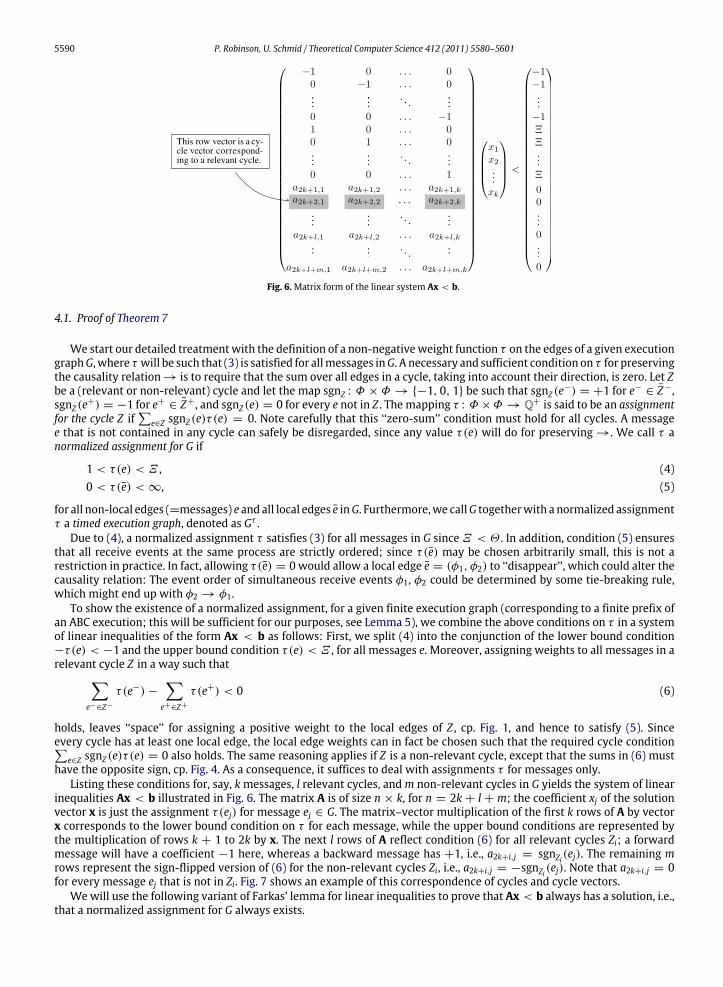
Fig. 6. Matrix form of the linear system Ax < b.

4.1. Proof of Theorem 7

We start our detailed treatmentwith the definition of a non-negativeweight function τ on the edges of a given executiongraphG, where τ will be such that (3) is satisfied for allmessages inG. A necessary and sufficient condition on τ for preservingthe causality relation→ is to require that the sum over all edges in a cycle, taking into account their direction, is zero. Let Zbe a (relevant or non-relevant) cycle and let the map sgnZ : Φ ×Φ → −1, 0, 1 be such that sgnZ (e−) = +1 for e− ∈ Z−,sgnZ (e+) = −1 for e+ ∈ Z+, and sgnZ (e) = 0 for every e not in Z . The mapping τ : Φ×Φ → Q+ is said to be an assignmentfor the cycle Z if

∑e∈Z sgnZ (e)τ (e) = 0. Note carefully that this ‘‘zero-sum’’ condition must hold for all cycles. A message

e that is not contained in any cycle can safely be disregarded, since any value τ(e) will do for preserving→. We call τ anormalized assignment for G if

1 < τ(e) < Ξ , (4)0 < τ(e) <∞, (5)

for all non-local edges (=messages) e and all local edges e inG. Furthermore,we callG togetherwith a normalized assignmentτ a timed execution graph, denoted as Gτ .

Due to (4), a normalized assignment τ satisfies (3) for all messages in G sinceΞ < Θ . In addition, condition (5) ensuresthat all receive events at the same process are strictly ordered; since τ(e) may be chosen arbitrarily small, this is not arestriction in practice. In fact, allowing τ(e) = 0 would allow a local edge e = (φ1, φ2) to ‘‘disappear’’, which could alter thecausality relation: The event order of simultaneous receive events φ1, φ2 could be determined by some tie-breaking rule,which might end up with φ2 → φ1.

To show the existence of a normalized assignment, for a given finite execution graph (corresponding to a finite prefix ofan ABC execution; this will be sufficient for our purposes, see Lemma 5), we combine the above conditions on τ in a systemof linear inequalities of the form Ax < b as follows: First, we split (4) into the conjunction of the lower bound condition−τ(e) < −1 and the upper bound condition τ(e) < Ξ , for all messages e. Moreover, assigning weights to all messages in arelevant cycle Z in a way such that−

e−∈Z−τ(e−)−

−e+∈Z+

τ(e+) < 0 (6)

holds, leaves ‘‘space’’ for assigning a positive weight to the local edges of Z , cp. Fig. 1, and hence to satisfy (5). Sinceevery cycle has at least one local edge, the local edge weights can in fact be chosen such that the required cycle condition∑

e∈Z sgnZ (e)τ (e) = 0 also holds. The same reasoning applies if Z is a non-relevant cycle, except that the sums in (6) musthave the opposite sign, cp. Fig. 4. As a consequence, it suffices to deal with assignments τ for messages only.

Listing these conditions for, say, kmessages, l relevant cycles, andm non-relevant cycles in G yields the system of linearinequalities Ax < b illustrated in Fig. 6. The matrix A is of size n × k, for n = 2k + l + m; the coefficient xj of the solutionvector x is just the assignment τ(ej) for message ej ∈ G. The matrix–vector multiplication of the first k rows of A by vectorx corresponds to the lower bound condition on τ for each message, while the upper bound conditions are represented bythe multiplication of rows k + 1 to 2k by x. The next l rows of A reflect condition (6) for all relevant cycles Zi; a forwardmessage will have a coefficient −1 here, whereas a backward message has +1, i.e., a2k+i,j = sgnZi(ej). The remaining mrows represent the sign-flipped version of (6) for the non-relevant cycles Zi, i.e., a2k+i,j = −sgnZi(ej). Note that a2k+i,j = 0for every message ej that is not in Zi. Fig. 7 shows an example of this correspondence of cycles and cycle vectors.

We will use the following variant of Farkas’ lemma for linear inequalities to prove that Ax < b always has a solution, i.e.,that a normalized assignment for G always exists.


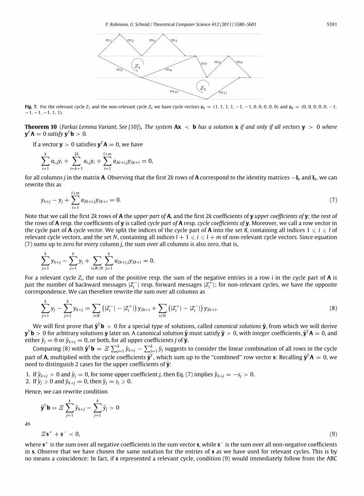
Fig. 7. For the relevant cycle Z1 and the non-relevant cycle Z2 we have cycle vectors z1 = (1, 1, 1, 1,−1,−1, 0, 0, 0, 0, 0) and z2 = (0, 0, 0, 0, 0,−1,−1,−1,−1, 1, 1).

Theorem 10 (Farkas Lemma Variant, See [10]). The system Ax < b has a solution x if and only if all vectors y > 0 whereyTA = 0 satisfy yTb > 0.

If a vector y > 0 satisfies yTA = 0, we havek−

i=1

ai,jyi +2k−

i=k+1

ai,jyi +l+m−i=1

a2k+i,jy2k+i = 0,

for all columns j in the matrix A. Observing that the first 2k rows of A correspond to the identity matrices−Ik and Ik, we canrewrite this as

yk+j − yj +l+m−i=1

a2k+i,jy2k+i = 0. (7)

Note that we call the first 2k rows of A the upper part of A, and the first 2k coefficients of y upper coefficients of y; the rest ofthe rows of A resp. the coefficients of y is called cycle part of A resp. cycle coefficients of y. Moreover, we call a row vector inthe cycle part of A cycle vector. We split the indices of the cycle part of A into the set R, containing all indices 1 ⩽ i ⩽ l ofrelevant cycle vectors, and the set N , containing all indices l + 1 ⩽ i ⩽ l + m of non-relevant cycle vectors. Since equation(7) sums up to zero for every column j, the sum over all columns is also zero, that is,

k−j=1

yk+j −k−

j=1

yj +−i∈R∪N

k−j=1

a2k+i,jy2k+i = 0.

For a relevant cycle Zi, the sum of the positive resp. the sum of the negative entries in a row i in the cycle part of A isjust the number of backward messages |Z−i | resp. forward messages |Z+i |; for non-relevant cycles, we have the oppositecorrespondence. We can therefore rewrite the sum over all columns as

k−j=1

yj −k−

j=1

yk+j =−i∈R

|Z−i | − |Z

+

i |y2k+i +

−i∈N

|Z+i | − |Z

−

i |y2k+i. (8)

We will first prove that yTb > 0 for a special type of solutions, called canonical solutions y, from which we will deriveyTb > 0 for arbitrary solutions y later on. A canonical solution y must satisfy y > 0, with integer coefficients, yTA = 0, andeither yj = 0 or yk+j = 0, or both, for all upper coefficients j of y.

Comparing (8) with yTb = Ξ∑k

j=1 yk+j −∑k

j=1 yj suggests to consider the linear combination of all rows in the cyclepart of A, multiplied with the cycle coefficients yT , which sum up to the ‘‘combined’’ row vector s: Recalling yTA = 0, weneed to distinguish 2 cases for the upper coefficients of y:

1. If yk+j > 0 and yj = 0, for some upper coefficient j, then Eq. (7) implies yk+j = −sj > 0.2. If yj ⩾ 0 and yk+j = 0, then yj = sj ⩾ 0.

Hence, we can rewrite condition

yTb = Ξk−

j=1

yk+j −k−

j=1

yj > 0

as

Ξs+ + s− < 0, (9)

where s+ is the sum over all negative coefficients in the sum vector s, while s− is the sum over all non-negative coefficientsin s. Observe that we have chosen the same notation for the entries of s as we have used for relevant cycles. This is byno means a coincidence: In fact, if s represented a relevant cycle, condition (9) would immediately follow from the ABC


synchrony condition (2).12 Even though s is not a cycle vector in general, since its coefficients are usually not in 0,±1, wewill exploit the fact that s is always a non-negative integer (since y > 0) linear combination of relevant and non-relevantcycles. Since we will prove (9) separately for non-negative linear combinations of relevant and non-relevant cycles, we splitΞs+ + s− < 0 into two parts:

Ξs+ + s− = Ξs+R + s−R + Ξs−N + s+N ,

where s+R , s−

R , s+

N , s−

N , are the appropriate restrictions to the index sets R and N . Bear in mind that the sign of the coefficientsof non-relevant cycle vectors are opposite to the relevant case.

Lemma 7 proves (9) for the non-relevant part; Lemma 11 will show the same result for the relevant part.

Lemma 7 (Non-Relevant Sum Property). Let z1, . . . , zℓ, ℓ ⩾ 1, be cycle vectors representing non-relevant cycles and let sN bethe vector corresponding to a non-negative linear combination of z1, . . . , zℓ. Then, it holds thatΞs−N + s+N < 0.

Proof. Since |Z−i |−|Z+

i | ⩾ 0 for every i, it follows immediately, by summing up, that every non-negative linear combinationsN also satisfies |s−N | − |s

+

N | ⩾ 0. SinceΞ > 1, this impliesΞs−N + s+N < 0.

Unfortunately, proving (9) for the relevant part is much more involved. The reason for this is that coefficients withopposite sign in a row cancel; this situation occurs in case of edge e in Fig. 2, for example. As a consequence, we cannotcarry over the ABC synchrony condition (2) that holds for every constituent cycle vector to their sum (9). In order to solvethis problem, we will show that there is a way to get rid of such cancellations, by constructing an equivalent set of cyclevectors that do not have coefficients with opposite sign in any row.

For proving Lemma 11, we will make use of some non-standard13 cycle space of the underlying execution graph G.Formally, the cycle-space C of G is the sub-space of the vector space of the edge sets in G over Q spanned by G’s (oriented)cycles. Since every cycle Zi corresponds to a unique set of messages in G, which can be uniquely identified by a k-tupleordered according to the columns in thematrix A, there is a one-to-one correspondence between cycles Zi in G and the cyclevectors zi in A, cp. Fig. 7. To avoid ambiguities w.r.t. indices, wewill usually denote the coefficient for message e in zi by (zi)e.Every cycle-space element

Z = λ1Z1 ⊕ λ2Z2 ⊕ · · · ⊕ λℓZℓis a linear combination of some relevant cycles Z1, . . . , Zℓ, with all coefficients λi ∈ Q, and the corresponding cycle vectorreads

z = λ1z1 + λ2z2 + · · · + λℓzℓ.Note that we will use both representations interchangeably in the sequel.

The cycle addition operation ⊕ is defined as follows: If the cycles Z1, Z2 corresponding to the cycle vectors z1, z2 aredisjoint, i.e., Z1 ∩ Z2 = ∅, then the cycle-space element

Z = Z1 ⊕ Z2 = Z1 ∪ Z2is the union of the two cycles Z1, Z2; it corresponds to the sum of the cycle vectors z = z1+ z2. Note that disjoint cycles mayhave common vertices (and even partially overlapping local edges), but no commonmessages. If the cycles have a commonmessage e, the outcome of adding z1 and z2 depends on the cycle vector orientation of Z1 and Z2: If e is oppositely oriented inZ1 and Z2, formally (z1)e · (z2)e < 0 [we also say that e is a mixed edge, i.e., e ∈ Z−1 ∩ Z+2 or e ∈ Z+1 ∩ Z−2 in relevant cycles,cp. message e in Fig. 2], then the coefficients cancel and hence (z)e = 0. Consequently, e is no longer present in Z = Z1⊕ Z2.Otherwise, if e is identically oriented in Z1 and Z2, formally (z1)e · (z2)e > 0 [we say that message e is either a forward or abackward edge in both cycles], then the coefficients do not cancel and (z)e = 0. In this case, e becomes a double edge inZ = Z1 ⊕ Z2.

Hence, in general, the subgraph Z = Z1 ⊕ Z2 corresponding to z = z1 + z2 is not a cycle, and Z1 ⊕ Z2 = Z1 ∪ Z2. In fact,the general cycle-space element

Z = λ1Z1 ⊕ · · · ⊕ λnZnis made up of multi-edges e with arbitrary multiplicity that is,

(z)e = λ1(z1)e + · · · + λn(zn)e ∈ Q.

We will show, however, that every non-negative integer linear combination of cycle vectors representing relevant cyclesyields a ‘‘relevant cycle like’’ vector z, in the sense that its coefficients satisfy the ABC synchrony assumption (2). Thisimmediately impliesΞs+R + s−R < 0 and thus proves (9) for the relevant part, see Lemma 11.

We start with the following Definition 10 of consistent cycles, which are such that all common edges consistently haveeither the same or the opposite orientation.

12 If s corresponds to a relevant cycle S, the definition of the cycle vector coefficients yields |S−| = s− and |S+| = −s+ and hence −Ξs+ − s− =Ξ |S+| − |S−| > 0 by (2).13 Our ‘‘cycle space’’ is quite different from the well known cycle space in graph theory, cp. [14], since our notion of ‘‘cycles’’ correspond to cycles in theundirected shadow graph while still taking edge orientation into account.


Definition 10 (Consistent Cycles). The cycles Z1 and Z2 are consistent, if there is some d ∈ −1,+1 such that the entries inthe corresponding cycle vectors satisfy (z1)e · (z2)e = d for all messages e ∈ Z1 ∩ Z2. If d = +1 resp. d = −1, then Z1 and Z2are called i-consistent (identically consistent) resp. o-consistent (oppositely consistent). If Z1 and Z2 are disjoint, then theyare i-consistent by definition. A set of cyclesM1, . . . ,Mn is consistent [i-consistent/o-consistent] w.r.t. a cycle Z , ifMi and Zare consistent [i-consistent/o-consistent], for every 1 ⩽ i ⩽ n.

For convenience, we say that Z1 ∩ Z2 contains resp. consists of oppositely oriented messages, if for some resp. everymessage e ∈ Z1 ∩ Z2 it holds that (z1)e · (z2)e = −1. We proceed with several technical lemmas devoted to the removal ofmixed edges in sums of cycle vectors.

Lemma 8 (Mixed Edge Removal (Two Cycles)). Let Z1 and Z2 be o-consistent cycles, such that all common message chainsm1, . . . ,mn in Z1∩Z2 consist of oppositely orientedmessages only. Then, there are disjoint cyclesM1, . . . ,Mn that are i-consistentw.r.t. both Z1 and Z2, such that Z1 ⊕ Z2 = M1 ⊕ · · · ⊕Mn. Moreover,

|M1 ⊕ · · · ⊕Mn| = |Z1 ⊕ Z2| − 2n−

i=1

|mi|.

Proof. Let Z1 = v1m1v′

1 . . . v2m2v′

2 . . . vn−1mn−1v′

n−1 . . . vnmnv′n . . . v1, where vi and v′i denote the vertices incident to the

message chain mi, be the sequence of vertices and edges of Z1 listed according to its cycle vector orientation. Since Z2traverses all common edges in the opposite direction, its analogous representation reads

Z2 = v′nmnvn . . . v′

n−1mn−1vn−1 . . . v′

2m2v2 . . . v′

1m1v1 . . . v′

n.

Hence, the chainsm1, . . . ,mn are cancelled in Z1 ⊕ Z2, only leaving the disjoint cycles

M1 = v1 . . . v′

n . . . v1,

M2 = v2 . . . v′

1 . . . v2,...

Mn = vn . . . v′

n−1 . . . vn.

Every Mi = vi . . . v′

i−1 . . . vi (with v′0 = v′n) consists of exactly one chain of messages v′i−1 . . . vi in Z1, and one chain ofmessages vi . . . v′i−1 in Z2, and is hence trivially i-consistent w.r.t. both Z1 and Z2.

Lemma 9 (Mixed Edge Removal (Single Set)). Let Z be a cycle. If M1, . . . ,Mn are disjoint cycles such that every Mi and Z areeither o-consistent or disjoint, then there is a set of disjoint cycles M ′1 . . . ,M

′

l′ , all of which are i-consistent w.r.t. Z , such thatMn ⊕ · · · ⊕M1 ⊕ Z = M ′1 ⊕ · · · ⊕M ′l′ .

Proof. We will construct M ′1 . . . ,M′

l′ recursively. For n = 1, if Z and M1 are disjoint (and hence i-consistent by definition),we just set M ′1 = Z , M ′2 = M1 and trivially get M1 ⊕ Z = M ′1 ⊕ M ′2. Otherwise, Z and M1 must be o-consistent and thestatement of our lemma follows immediately from Lemma 8, applied to Z andM1.

Now suppose that we have already constructed a set of disjoint cyclesM ′1, . . . ,M′

l′ that are all i-consistent w.r.t. Z with

Mn−1 ⊕ · · · ⊕M1 ⊕ Z = M ′1 ⊕ · · · ⊕M ′l′ .

Since⊕ is commutative and associative, it holds that

Mn ⊕Mn−1 ⊕ · · · ⊕M1 ⊕ Z = Mn ⊕M ′1 ⊕ · · · ⊕M ′l′ = M ′1 ⊕ . . . . . .M′

l′ ⊕Mn.

By our hypothesis, every M ′ℓ, 1 ⩽ ℓ ⩽ l′, and Z are i-consistent, whereas Mn and Z are either disjoint or o-consistent. Itfollows immediately that everyM ′ℓ andMn is either o-consistent or disjoint. Since these are exactly the preconditions of ourlemma, our recursive construction can be applied again. The termination of this recursive construction is guaranteed, sinceevery application of Lemma 8 reduces the number of edges in the result.

Lemma 10 (Mixed Edge Removal (General Set)). Let Z1, . . . , Zn be a set of cycles such that, for 1 ⩽ i < j ⩽ n, cycles Zi and Zjare either disjoint or o-consistent. Then, there exist disjoint cycles M1, . . . ,Ml that are all i-consistent w.r.t. every Zi, 1 ⩽ i ⩽ n,such that Z1 ⊕ · · · ⊕ Zn = M1 ⊕ · · · ⊕Ml.

Proof. The proof is by induction. For n = 1, Z1 andM1 = Z1 are trivially i-consistent, hence establishing the induction base.For the induction step, suppose that there are disjoint cycles M1, . . . ,Ml that are i-consistent w.r.t. every Zi, 1 ⩽ i ⩽ n− 1,such that

Z1 ⊕ · · · ⊕ Zn−1 = M1 ⊕ · · · ⊕Ml.

Now, since every Mℓ, 1 ⩽ ℓ ⩽ l, and every Zi, 1 ⩽ i ⩽ n − 1, are i-consistent, whereas every Zi and Zn are o-consistent,it follows immediately that every Mℓ and Zn is either o-consistent or disjoint. Hence, we can apply Lemma 9 with Z = Zn,which provides the required set M ′1, . . . ,M

′

l′ of disjoint cycles that are i-consistent w.r.t. every Zi, 1 ⩽ i ⩽ n and satisfyM ′1 ⊕ · · · ⊕M ′l′ = Z1 ⊕ · · · ⊕ Zn as required.


Theorem 11 (Mixed-Free Decomposition). Let C ∈ C be a cycle-space element such that C = Z1 ⊕ · · · ⊕ Zn. Then, there arecycles M1, . . . ,Ml, which are all i-consistent w.r.t. every Zi, 1 ⩽ i ⩽ n and noMj∩Mj′ , 1 ⩽ j < j′ ⩽ l, contains oppositely orientedmessages, such that

Z1 ⊕ · · · ⊕ Zn = M1 ⊕ · · · ⊕Ml.

Proof. Let Γ be any non-empty subset of the multi-edges in C , i.e., of messages e that have some integer coefficient(c)e ∈ 0,±1 in the cycle vector corresponding to C . We can define an extended cycle-space C[Γ ] as follows: Given somemulti-edge e ∈ Γ , there must be at least k = |(c)e| cycles Zπ1 , . . . , Zπk where e has the same orientation d = sgn((c)e) =sgn((zπi)e), 1 ⩽ i ⩽ k. For every such Zπi , we introduce a new edge labeled eZπi and replace Zπi by Z ′πi , where (z′πi)e = 0 but(z′πi)eZπi = d. Doing this for all e ∈ Γ provides a new set of cycles Z1[Γ ], . . . , ZnΓ [Γ ] ∈ C[Γ ], which sum up to

C[Γ ] = Z1[Γ ] ⊕ · · · ⊕ ZnΓ [Γ ].

Note that the only difference between C and C[Γ ] is that we have split all multi-edges ∈ Γ occurring in C into separatenew edges (which all have coefficients ∈ 0,±1) in C[Γ ]. Let Γ ∗ denote the set of all multi-edges in C; note that Γ ⊂ Γ ∗implies that C[Γ ] still contains multi-edges in Γ ∗\Γ .

We will now prove by means of backwards induction on |Γ | that the statement of our theorem actually holds for everycycle-space element C[Γ ]. Since C[∅] = C , this will also prove Theorem 11.

For the induction base, let Γ = Γ ∗. Since all multi-edges have been split in C[Γ ∗], every pair Zi[Γ ∗], Zj[Γ ∗], 1 ⩽ i < j ⩽

nΓ∗

, is either disjoint or o-consistent. Lemma 10 thus reveals that there are disjoint cycles M1[Γ∗], . . . ,Mk[Γ

∗] ∈ C[Γ ∗]

that are all i-consistent w.r.t. every Zi[Γ ∗], where

M1[Γ∗] ⊕ · · · ⊕Mk[Γ

∗] = Z1[Γ ∗] ⊕ · · · ⊕ ZnΓ ∗ [Γ

∗]

as required. Note that noMi[Γ∗] ∩Mj[Γ

∗] can contain oppositely oriented messages because they are disjoint.

For the induction step, we assume that there are cyclesM ′1[Γ ], . . . ,M′

k[Γ ] ∈ C[Γ ], which are all i-consistent w.r.t. everyZi[Γ ], 1 ⩽ i ⩽ nΓ and noM ′j [Γ ] ∩M ′j′ [Γ ], 1 ⩽ j < j′ ⩽ k, contains oppositely oriented messages, such that

M ′1[Γ ] ⊕ · · · ⊕M ′k[Γ ] = C[Γ ].

Let M ′j [Γ ], 1 ⩽ j ⩽ k, be such a cycle. Suppose that M ′j [Γ ] contains α ⩾ 1 ‘‘instances’’ of a multi-chain c ⊆ Γ , i.e., αmaximum-length chains cZ1 , . . . , cZα which have all been obtained by introducing new edges for the multi-edges makingup the singlemulti-chain c. W.l.o.g., we can write

M ′j [Γ ] = vZ11 cZ1vZ12 . . . v

Z21 cZ2vZ22 . . . v

Zα1 cZαvZα2 . . . v

Z11 .

Consequently, we have the following chains inM ′j [Γ ]:

vZ11 cZ1vZ12 . . . v

Z21 cZ2 = Mj1c

Z2 ,

vZ21 cZ2vZ22 . . . v

Z31 cZ3 = Mj2c

Z3 ,...

vZα1 cZαvZα2 . . . v

Z11 cZ1 = Mjα c

Z1 .

Now, if we rejoin all the edges in cZ1 , . . . , cZα to form the multi-chain c again, that is, if we make a transition from C[Γ ] toC[Γ \c], then all instances of cZ1 , . . . , cZα in the above chains collapse to the single multi-chain c. Consequently, in C[Γ \c],every of the Mjℓ , 1 ⩽ ℓ ⩽ α, above actually forms a cycle Mjℓ [Γ \c] — note that the vertices vZℓ1 and vZℓ+11 also collapse toa single vertex. Since M ′j [Γ ] is i-consistent w.r.t. every Zi[Γ ], 1 ⩽ i ⩽ nΓ , every Mjℓ [Γ \c]must be i-consistent w.r.t. everyZi[Γ \c], 1 ⩽ i ⩽ nΓ \c , as well. Furthermore, according to the construction above, every edge of M ′j [Γ ] (except the edgesin cZ1 , . . . , cZα , of course) is contained in exactly one cycle Mjℓ [Γ \c], and no Mjℓ [Γ \c] ∩ Mjℓ′ [Γ \c] can contain oppositelyoriented edges. Finally, noMiℓ [Γ \c]∩Mjℓ′ [Γ \c], i = j, can contain oppositely oriented edges either, sinceM ′j [Γ ] andM ′i [Γ ]are disjoint. Hence, taking all the setsMjℓ [Γ \c] (or, if α = 0 forM ′j [Γ ], then Mj[Γ \c] := M ′j [Γ ]) provides the sought set

M1[Γ \c], . . . ,Mk[Γ \c] ∈ C[Γ \c],

thereby completing our proof.

Corollary 1. Let C ∈ C be such that C = Z1 ⊕ · · · ⊕ Zn, for relevant cycles Z1, . . . , Zn. Then,|C−||C+| < Ξ .

Proof. Applying Theorem 11 yields cyclesM1, . . . ,Ml such that

C = Z1 ⊕ · · · ⊕ Zn = M1 ⊕ · · · ⊕Ml,

which do not contain oppositely oriented messages that would cancel when summing up. In order to prove |C−|

|C+| < Ξ , it

hence suffices to show |M−i |

|M+i |< Ξ for everyMi. There are only two possibilities:


1. M−i ⊆ C−,M+i ⊆ C+: If Mi is relevant, then obviously |M−

i |

|M+i |< Ξ . Assume, for the sake of contradiction, that Mi

is non-relevant. Then there is a local edge κ ∈ Mi that is traversed forward (causally) in Mi, and hence in C . SinceC = Z1 ⊕ · · · ⊕ Zn, there must be some Zj with κ ∈ Zj where κ is traversed in the same way as in C and, hence, inMi. This contradicts Zj being a relevant cycle, however.

2. M+i ⊆ C−,M−i ⊆ C+: By (1), it holds that |M−i | ⩾ |M+i | and hence |M+

i |

|M−i |⩽ 1 < Ξ . Since M−i resp. M+ correspond to

edges in C+ resp. C−, it follows thatMi contributes properly to |C−|

|C+| < Ξ as required. Note that this holds independentlyof whether Mi is relevant or not.

This completes the proof of Corollary 1.

As a consequence, we finally get the desired proof of (9) for the relevant part:

Lemma 11 (Relevant Sum Property). Let z1, . . . , zℓ be cycle vectors representing relevant cycles and let sR be the vectorcorresponding to a non-negative integer linear combination of z1, . . . , zℓ. Then, it holds thatΞs+R + s−R < 0.

Proof. Corollary 1 does not require the Zi to be different. Since SR = λ1Z1⊕ · · ·⊕ λℓZℓ for non-negative integer coefficientsλi, we can hence invoke Corollary 1 with λi instances of the same relevant cycle Zi, 1 ⩽ i ⩽ ℓ.

Combining Lemmas 7 and 11 immediately proves that every canonical solution y satisfies yTb > 0. It only remains toextend this result to arbitrary solution vectors y, which is done in the following Theorem 12.

Theorem 12 (Existence of a Normalized Assignment). The system Ax < b corresponding to a finite execution graph has alwaysa solution, and hence a normalized assignment.

Proof. The statement follows immediately from Theorem 10, if we can show that every y > 0 with coefficients yj ∈ Qsatisfying yTA = 0 also fulfills yTb > 0. If y is a canonical solution y, then yTb > 0 follows from adding the results ofLemmas 7 and 11, recall (9) in conjunction withΞs+ + s− = Ξs+R + s−R +Ξs−N + s+N . Otherwise, we can derive a canonicalsolution y from a non-canonical solution y as follows:

1. For all upper coefficients 1 ⩽ j ⩽ k of y: If yj > yk+j, then yj = yj − yk+j and yk+j = 0; otherwise, yk+j = yk+j − yj andyj = 0.

2. For all cycle coefficients 2k+ 1 ⩽ i ⩽ 2k+ l+m of y: yi = yi.3. Finally, multiply every yj by the least common multiple of y1, . . . , y2k+l+m to get integer coefficients.

Since yTA = 0, it follows immediately from the above definition of y that yTA = 0. Hence, yTb > 0. Now consider(yT − yT )bT ; after cancelling the common parts of y and y, according to our construction, we get

(yT − yT )bT=

−j:yk+j⩾yj

(Ξ − 1) yj +−

j:yj>yk+j

(Ξ − 1) yk+j.

This term is non-negative, since y is non-negative andΞ > 1. Hence, yTb ⩾ yTb > 0 and we are done.

Theorem 12 immediately implies the sought Theorem 7.

5. Related work and practical aspects

In this section, we briefly relate the ABC model to the existing partially synchronous models (1)–(7) listed in Section 1and discuss some observations concerning the practical applicability of the model.

The fact that we will primarily discuss aspects where the ABC model surpasses alternative models should not be takenas a claim of general superiority, however: A fair model comparison is difficult and also highly application dependent; italmost always leads to the conclusion that any two models are incomparable, in the sense that model A is better than B inaspect X but worse in aspect Y , cp. [40]. We start with a brief account of the major features of those models.

The classic partially synchronous models introduced in Dwork et al. [17] and the semi-synchronous models from [36,7]incorporate a bound Φ on the relative speed of processes, in addition to a transmission delay bound ∆. All those modelsallow a process to timeout messages: The semi-synchronous models assume that local real-time clocks are available, theclassic partially synchronousmodels use the computing step time of the fastest process as the units of ‘‘real time’’; a spin loopwith loop count∆ is hence sufficient for timing out the maximummessage delay here. An even older partially synchronousmodel is the Archimedean model introduced in [39], which assumes a bounded ratio s ⩾ u/c of the minimum computingstep time c and the maximum computing step time + transmission delay u. Again, any process can timeout a message bymeans of a local spin loop with loop count s here.

An even more relaxed way of adding synchrony properties to asynchronous systems underlies the chase for the weakestsystemmodel for implementing theΩ failure detector in systemswith crash failures, see [3,2,4,34,6,30,26,27]; an extensionto Byzantine failures can be found in [1]. These Weak Timely Link (WTL) models can be viewed as a ‘‘spatial’’ relaxation ofthe classic partially synchronous or semi-synchronous models: The currently weakest of these models, introduced in [26,


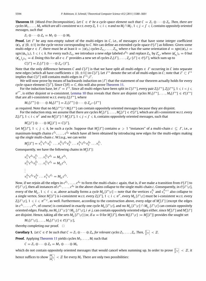
Fig. 8. A relevant cycle, valid for anyΞ > 1. Note that r takes no step while p and q can make progress only bounded by |Z−|.

27], requires just a single process p (a timely f -source) with f eventual timely outgoing links, connecting p to a time-variantset of f receiver processes. Note that communication over all the other links in the system can be totally asynchronous.

A model that is very close to pure asynchrony is the Finite Average Response time (FAR) model introduced in [21,22].The properties added to the FLP model are an unknown lower bound for the computing step time, and an unknown finiteaverage of the round-trip delays between any pair of correct processes. The latter allows round-trip delays to be increasingwithout bound, provided that there are sufficiently many short round trips in between that compensate for the resultingincrease of the average. Due to the computing step time lower bound, any process can implement a weak bounded driftclock via a local spin loop here, which allows to safely timeout messages by using timeout values learned at runtime.

The remaining models MCM and MMR will be described in Section 5.2.

5.1. Relation to the classic partially synchronous model

In this section, we relate the ABCmodel to the classic partially synchronousmodel (abbreviated ParSync14) introduced inDwork et al. [17]. ParSync stipulates a boundΦ on relative computing speeds and a bound∆ on message delays, relative toan (external) discrete ‘‘global clock’’, which ticks whenever a process takes a step: During Φ ticks of the global clock, everyprocess takes at least one step, and if a message m was sent at time k to a process p that subsequently performs a receivestep at or after time k+∆, p is guaranteed to receivem.

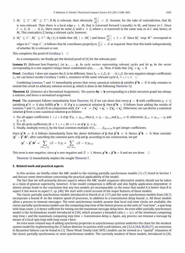
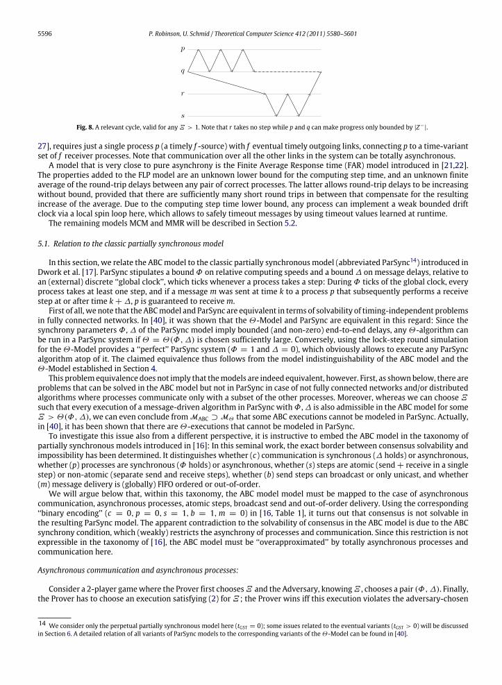
First of all, we note that the ABCmodel and ParSync are equivalent in terms of solvability of timing-independent problemsin fully connected networks. In [40], it was shown that the Θ-Model and ParSync are equivalent in this regard: Since thesynchrony parameters Φ ,∆ of the ParSync model imply bounded (and non-zero) end-to-end delays, anyΘ-algorithm canbe run in a ParSync system if Θ = Θ(Φ,∆) is chosen sufficiently large. Conversely, using the lock-step round simulationfor the Θ-Model provides a ‘‘perfect’’ ParSync system (Φ = 1 and ∆ = 0), which obviously allows to execute any ParSyncalgorithm atop of it. The claimed equivalence thus follows from the model indistinguishability of the ABC model and theΘ-Model established in Section 4.

This problemequivalence does not imply that themodels are indeed equivalent, however. First, as shownbelow, there areproblems that can be solved in the ABC model but not in ParSync in case of not fully connected networks and/or distributedalgorithms where processes communicate only with a subset of the other processes. Moreover, whereas we can choose Ξsuch that every execution of a message-driven algorithm in ParSync withΦ ,∆ is also admissible in the ABCmodel for someΞ > Θ(Φ,∆), we can even conclude from MABC ⊃MΘ that some ABC executions cannot be modeled in ParSync. Actually,in [40], it has been shown that there areΘ-executions that cannot be modeled in ParSync.

To investigate this issue also from a different perspective, it is instructive to embed the ABC model in the taxonomy ofpartially synchronous models introduced in [16]: In this seminal work, the exact border between consensus solvability andimpossibility has been determined. It distinguishes whether (c) communication is synchronous (∆ holds) or asynchronous,whether (p) processes are synchronous (Φ holds) or asynchronous, whether (s) steps are atomic (send+ receive in a singlestep) or non-atomic (separate send and receive steps), whether (b) send steps can broadcast or only unicast, and whether(m) message delivery is (globally) FIFO ordered or out-of-order.

We will argue below that, within this taxonomy, the ABC model model must be mapped to the case of asynchronouscommunication, asynchronous processes, atomic steps, broadcast send and out-of-order delivery. Using the corresponding‘‘binary encoding’’ (c = 0, p = 0, s = 1, b = 1,m = 0) in [16, Table 1], it turns out that consensus is not solvable inthe resulting ParSync model. The apparent contradiction to the solvability of consensus in the ABC model is due to the ABCsynchrony condition, which (weakly) restricts the asynchrony of processes and communication. Since this restriction is notexpressible in the taxonomy of [16], the ABC model must be ‘‘overapproximated’’ by totally asynchronous processes andcommunication here.

Asynchronous communication and asynchronous processes:

Consider a 2-player gamewhere the Prover first choosesΞ and the Adversary, knowingΞ , chooses a pair (Φ,∆). Finally,the Prover has to choose an execution satisfying (2) forΞ ; the Prover wins iff this execution violates the adversary-chosen

14 We consider only the perpetual partially synchronous model here (tGST = 0); some issues related to the eventual variants (tGST > 0) will be discussedin Section 6. A detailed relation of all variants of ParSync models to the corresponding variants of theΘ-Model can be found in [40].


Fig. 9. The long delay on the link between q and r is compensated by the fast delay on the link between r and s.

Fig. 10. A system implementing bounded-size FIFO channels. If the order of φ and φ′ is changed, there would be a relevant cycle violating (2) ifΞ = 4.

parameters (Φ,∆). The Prover has a winning strategy: It suffices to choose any execution containing a relevant cycle asshown in Fig. 8, which respects (2) but lets |Z−| be greater than both Φ and ∆: While the (slow) message from q to r is intransit, process q executesmore than∆ steps. Moreover, neither process r nor s execute a step during themore thanΦ stepsof q. As a consequence, both communication and processes must be considered asynchronous (c = 0, p = 0).

Atomic steps and broadcast:

Whereas it is clear that out-of-order delivery (m = 0) makes it more difficult to solve problems, one may be wonderingwhether the ‘‘favorable’’ choices s = 1 and b = 1, rather than the ABC synchrony condition, make consensus solvablein the ABC model. Dolev et al. [16, Table 1] reveals that this is not the case, however: All the entries corresponding top = 0, c = 0,m = 0 are the same (consensus impossible), irrespectively of the choice of b and s. And indeed, theassumption of atomic send + receive steps with broadcast in the ABC model’s definition in Section 2 is just a simplifyingabstraction: Every non-atomic unicast execution can bemapped to a causally equivalent atomic send+ receive+ broadcaststep execution with appropriately adjusted end-to-end delays. The ABC model can hence also be used for making classicdistributed algorithms results applicable to non-atomic models like the Real-Time Model introduced in [33].

Another major difference between ParSync and the ABC model results from the cumulative and dynamic, non-system-wide character of the ABC synchrony condition. Since (2) needs to hold only in relevant cycles, which are in fact defined bythe message patterns of the specific algorithm employed, the ABC model is particularly suitable for modeling systems withnot fully connected communication graphs: For choosingΞ , only the cumulative end-to-end delay ratio over certain pathscounts.

Consider the execution shown in Fig. 9, for example, which corresponds to a systemwhere process q exchangesmessagesdirectly with p (over a 1-hop path Pqpq), and indirectly with s (over a 2-hop path Pqrsrq via r). As long as the sum of the delaysalong Pqrsrq is less than the cumulative delay of Ξ instances of Pqpq, the individual delays along the links between q, r andr, s are totally irrelevant. In the VLSI context, for example, this gives more flexibility for place-and-route, as well as somerobustness against dynamic delay variations. By contrast, in ParSync, very conservative values of Φ ,∆ would be needed toachieve a comparable flexibility; obviously, this would considerably degrade the achievable performance system-wide.

In case of not fully connected networks, there are even situations which cannot be modeled in ParSync at all. Considerthe message pattern given in Fig. 10 in a system with Ξ = 4, for example: The ABC synchrony condition ensures FIFOorder of the messages sent from p2 to q1, even when their delay is unbounded (and may even continuously grow, as e.g. ina formation of fixed-constellation clusters of spacecraft that move away from each other): If there was a reordering of φand φ′, a relevant cycle with Ξ = 5 would be formed, which is not admissible for Ξ = 4 and hence cannot occur. Notethat processes p1, p2 make unbounded progress while a message to q1 is in transit here. Hence, as in the example of Fig. 8mentioned before, the problem cannot be solved in ParSync. Clearly, such message ordering capabilities are very useful inpractice, e.g., for implementing stable identifiers, bounded message size, single source FIFOs etc.

5.2. Relation to other partially synchronous models

In this section, wewill briefly relate the ABCmodel to the remaining partially synchronousmodels MCM andMMR listedin Section 1.

Whereas most existing partially synchronous models refer to message delays and computing step times, the ABC modelonly constrains the ratio of the number of backward vs. forward messages in relevant cycles. Moreover, the ABC modeldoes not assume any relation between computing step times andmessage delays, and, in contrast to the models consideredin Section 5.1, can also be used to model systems where no hardware clock is available. Note that this is also true for theFAR Model by Fetzer et al. [22], which requires a bounded-speed clock and hence introduces some (weak) dependency


between average message delays and computing steps as well. The only exceptions are theΘ-Model, which constrains themaximal/minimal end-to-end delay ratio, the MCMmodel by Fetzer [20] that assumes a classification of received messagesin ‘‘slow’’ and ‘‘fast’’ ones, and the MMR model of Mostefaoui et al. [35], which restricts the message order in round-tripcommunication patterns.

TheMCMmodel applies to systemswith process crash failures. It assumes that all receivedmessages are correctly flaggedas either ‘‘slow’’ or ‘‘fast’’, with the requirement that the end-to-end delay of any slow message is more than two times theend-to-end delay of any fast message. To prohibit flagging all messages as ‘‘slow’’, Fetzer [20] assumes the existence of atleast one correct process p that can eventually communicate bidirectionally with all correct processes via ‘‘fast’’ messages.Except for messages sent/received by this eventual bidirectional n-source p (in the terminology of the WTL models), theMCMmodel also allowsmessage loss and even transient partitioning. Since themessage classification assumption facilitatesa time-free timeout mechanism for ‘‘fast’’ round trips (by means of local messages, sent from a process to itself, which arealways delivered as ‘‘slow’’), the MCM model allows the implementation of the eventually strong failure detector S and,hence, to solve consensus.

Like the ABC model, the MCM model is totally time-free, yet allows to reliably timeout certain messages. However,whereas the MCM uses local ‘‘slow’’ messages to timeout a round-trip of ‘‘fast’’ ones, the ABC model uses ‘‘fast’’ messagechains to timeout ‘‘slow’’ ones.15 The message classification assumption is hence more demanding than the ABC condition,since no two messages with delay ratio in the interval (1, 2] may ever be in transit simultaneously (unless they are both‘‘slow’’).

The MMR model by Mostefaoui et al. [35] also applies to systems with at most f process crash failures. It assumes that,in every round-trip of process pi with all its peers, there is a fixed set of processes Qi the responses of which are among thefirst n− f responses received by pi. This property turned out to be sufficient for implementing the eventually strong failuredetector S and, hence, to solve consensus.

Like theABC condition, theMMRcondition enforces a certain order of events. Although this condition cannot be expressedexplicitly in the ABC model, it can be interpreted as a special instance of the (undefined16) situation Ξ = 1 for certainmessages. Due to its order-based synchrony condition, the MMR model shares several advantages of the ABC; on the downside, it is restricted to a specific communication pattern and has a quite demanding synchrony requirement (albeit for certainmessages only). Moreover, the ABC model is superior w.r.t. solvability of problems, since the MMRmodel does not allow toreliably timeout messages. It is hence impossible to implement uniform lock-step rounds, for example: If a process q sendsa roundmessage to p and then immediately crashes, p cannot distinguish this from the scenario where q has crashed beforesending the round message. Consequently, neither Lemma 4, which gives a bound on the failure detection time, nor thebounded progress condition in Theorem 4 could be derived in the MMRmodel. Actually, the same is true for any model thatdoes not provide stronger synchrony properties than provided by a perfect failure detector, i.e., for any model where theStrongly Dependent Decision Problem cannot be solved, see [12].

A particularly attractive property of the ABC model is its ability to deal with unbounded message delays. Among theexisting partially synchronousmodels, this is also true for theMCMmodel, theMMRmodel, the FARModel and the dynamicΘ-Model introduced in [40]. The FAR Model actually surpasses the ABC model here, in the sense that it does not requireany correlation between the delays of messages exchanged by different processes. On the other hand, the FAR Model isinferior to the ABC model due to its requirement of finite average message delays, which rules out continuously growingdelays (occurring e.g. in a formation of spacecraft that continuously move away from each other). The remaining partiallysynchronous models also allow growing delays, although all message delays must change roughly at the same rate. Bycontrast, as already mentioned in Section 5.1, the ABC model does not force unrelated messages to meet any constraints,and even allows messages with zero delay.

5.3. Practical aspects

Since the ABC model shares many features with the Θ-Model, most of the applicability and model coverage aspectsdiscussed in [40] apply a fortiori to the ABC model. In particular, as a message-driven model, the ABC model suffers fromthe problem that the entire system may become mute in case of excessive message loss and/or partitioning, and that theoverhead of continuously sendingmessages may become significant. Although there are ways of mitigating these problems,they cannot be ruled out completely. At the same time, ABC algorithms are easily portable and benefit from the ABCmodel’sgood coverage in real systems.

Moreover, the non-system-wide scope of the ABC synchrony condition (2), which only constrains messages in relevantcycles on a per-cycle basis, makes the ABC model also applicable to in systems that cannot be modeled by the existingpartially synchronous models. Consider a formation of spacecraft, for example, where clusters of spacecraft continuouslymove away from each other but stay closewithin a cluster: If an algorithm generates onlymessage chains that spanmultiple

15 Note that, in contrast to the MCMmodel, in the ABC model there is no global classification of messages into ‘‘fast’’ and ‘‘slow’’ messages, as a ‘‘fast’’ (i.e.backward, see Definition 3) message in one cycle Z might actually be a ‘‘slow’’ (i.e. forward) message in another cycle Y .16 Since this would make the definition of forward and backward edges (and hence of relevant and irrelevant cycles) superfluous, the ABC model doesnot allowΞ = 1.


clusters in relevant cycles, a properly chosen ABC synchrony condition in the corresponding execution graph will alwaysbe maintained. No existing partially synchronous model can adequately model such systems: The DLS Model Dwork et al.[17], the Archimedean Model Vitányi [38] and the WTL Models Aguilera et al. [4,30,26] assume some (possibly unknown)global delay bound for all timelymessages. TheΘ-Model [40], on the other hand, suffers from the problem that allmessagessimultaneously in transit within the whole system must obey the global delay ratio Θ . Somewhat an exception is the FARModel, which does not require any correlation between the delays of messages exchanged by different processes; it fails tomodel the above example just because of the ever-growing delays, however.

Interestingly, the ABC model is also a promising candidate for modeling distributed algorithms in very large scaleintegration (VLSI) circuits17: Due to continuously shrinking feature sizes and increasing clock speeds, today’s deep sub-micron VLSI have much in common with loosely coupled asynchronous distributed systems studied in distributedcomputing for decades, see e.g. [37,18]. Given that the delays observed in a particular chip depend heavily on the VLSIimplementation technology, as well as on the actual place-and-route of the components and wires, it is definitely sub-optimal to compile timevalues into a distributed algorithmhere—inparticular,when those values affect its internal structure(message-buffer sizes, for example): Re-using such an algorithm in conjunctionwith a different implementation technologyor within a different application would be difficult.

By contrast, when an ABC algorithm is used in the VLSI context, there is a very good chance that the algorithm canbe re-used without a change. In particular, when a design is migrated to a, say, faster implementation technology, bothminimum and maximum delay paths are usually sped up in a similar way. Hence, the algorithm’s Ξ is likely18 to continueto hold. Similarly, if an ABC algorithm is employed within a different VLSI application, one can usually guarantee its Ξ bysetting suitable constraints during place-and-route. Thanks to the ABC model’s weak properties, these constraints concern(1) cumulative delays, and (2) timing ratios only. They are hence much easier to satisfy than explicit timing constraints puton individual components and wires.

6. Weaker variants of ABC models

Analogous to Dwork et al. [17] and Widder and Schmid [40], it is possible to define 4 variants of the ABC model:

• ABC model:Ξ is known and holds perpetually (the model introduced in Section 2)• ?ABC model:Ξ is unknown and holds perpetually• ABC model:Ξ is known and holds eventually• ?ABC model:Ξ is unknown and holds eventually

In case of the latter twomodels, we assume that only relevant cycles starting at or after some (unknown) consistent cutCGST(replacing the ‘‘global stabilization time’’ in Dwork et al. [17]) in the execution graph satisfy (2).

Due to the ‘‘indistinguishability’’ of the ABC model and theΘ-Model forΘ-algorithms, established in Section 4, one canimmediately use the algorithms proposed in [40] for providing eventual lock-step rounds in the ?Θ-, Θ-, and ?Θ-Modelsto achieve the same in the ?ABC model, ABC model, and ?ABC model.

In case of the ?ABC model and the ?ABC model, the resulting algorithms are not particularly efficient, however, sincethey double the round duration with every round. A more clever algorithm could exploit the ABC synchrony condition toeventually learn a feasible value for Ξ : Suppose p’s current estimate Ξ of Ξ is 2 in the execution depicted in Fig. 3. In thecomputing step ψ , process p finds out that either Ξ = 2 is wrong or pslow has crashed; it can hence increase its estimateΞ as soon as the slow message from pslow arrives. The definition and analysis of such refined algorithms is a subject of ourcurrent research.

An orthogonal way of weakening the ABC model is to drop all cycles from the space–time diagram that exceed a certainlength. For example Algorithm 1 will work correctly even in an ABC model where only cycles with at most 2 forwardmessages are considered.

A related, particularly interesting topic of our current research is consensus solvability in the ABC model: Obviously, ontop of the lock-step round simulation in the ABC model, any Byzantine fault-tolerant synchronous consensus algorithm canbe used for solving consensus. Similarly, on top of the eventual lock-step round simulations in the ?ABC model, the ABCmodel, and the ?ABC model, consensus can be solved with the Byzantine resilient algorithms introduced in Dwork et al.[17].

It is still an open question, however, whether the ABC model can contribute another step beyond the currently weakestmodel by Hutle et al. [27] for solving consensus in the presence of crash failures. Both the time freeness and the non-system-wide scope of the ABC synchrony condition make it a promising candidate. However, answering this question boils downto finding ‘‘minimum’’ execution graphs (recall Section 2), i.e., ways of dropping almost all messages (and hence exempting

17 Which is an emerging field, see e.g. the Dagstuhl seminar Fault-Tolerant Distributed Algorithms in VLSI Chips organized by Charron-Bost et al. [13].18 For example, we succeeded to migrate the DARTS fault-tolerant clock generation algorithm for Systems-on-Chip (see [24,19]), which is based onAlgorithm 1, from an FPGA to a high-speed ASIC without a change.


them from the ABC synchrony condition) except for a minimal set that cannot be dropped without running into the FLPimpossibility.

For example, one could just adopt the idea underlying the simple Ω failure detector Chandra and Toueg [11] forthe Θ-Model [9]: The ABC synchrony condition could be restricted to a fixed subset of f + 2 processes in the system,which elect a leader among themselves and disseminate its id to the remaining processes in the system. By virtue ofour ‘‘model indistinguishability’’ result, it immediately follows that the algorithms of Biely and Widder [9] are correct Ω-implementation in the ABC model as well. Similarly, using a straightforward extension of the ABC model to time-drivensystems, it would also possible to adapt theΩ-implementations developed for the WTL models to the ABC model.

7. Conclusions and future work

We have introduced a novel partially synchronous system model, the ABC model, which is completely time-free andthus rests on a causality-based synchrony condition only. We showed that it is sufficiently strong for implementing lock-step rounds and, hence, for solving important distributed computing problems, including consensus. We also proved thatalgorithms designed for the Θ-Model also work correctly in the ABC model. Our results thus reveal that explicit timingconstraints are not essential for a synchrony-based approach, even if failure detector oracles or randomization are notavailable. Part of our future work is devoted to fully exploiting the ABC model in the chase for the weakest system modelfor solving consensus, and to the analysis of the ABC model’s coverage in real systems, in particular, VLSI Systems-on-Chip.

Acknowledgements

We are most indebted to Martin Biely, Josef Widder, Martin Hutle, Matthias Függer, Heinrich Moser, and BernadetteCharron-Bost for their contributions to the development of the ABC model.

References

[1] Marcos K. Aguilera, CaroleDelporte-Gallet, Hugues Fauconnier, SamToueg, Consensuswith Byzantine failures and little system synchrony, in: DSN ’06:Proceedings of the International Conference on Dependable Systems and Networks, IEEE Computer Society, Washington, DC, USA, 2006, pp. 147–155.doi:10.1109/DSN.2006.22. ISBN 0-7695-2607-1.

[2] Marcos K. Aguilera, Carole Delporte-Gallet, Hugues Fauconnier, Sam Toueg, On implementing omega in systems with weak reliability and synchronyassumptions, Distributed Computing 21 (4) (2008).

[3] Marcos Kawazoe Aguilera, Carole Delporte-Gallet, Hugues Fauconnier, Sam Toueg, Stable leader election, in: DISC’01: Proceedings of the 15thInternational Conference on Distributed Computing, Springer-Verlag, 2001, pp. 108–122. ISBN 3-540-42605-1.

[4] Marcos Kawazoe Aguilera, Carole Delporte-Gallet, Hugues Fauconnier, Sam Toueg, Communication-efficient leader election and consensus withlimited link synchrony, in: Proceedings of the 23th ACM Symposium on Principles of Distributed Computing, PODC’04, ACM Press, St. John’s,Newfoundland, Canada, 2004, pp. 328–337. doi:10.1145/1011767.1011816. ISBN 1-58113-802-4.

[5] Bowen Alpern, Fred B. Schneider, Defining liveness, Information Processing Letters 21 (4) (1985) 181–185.[6] Emmanuelle Anceaume, Antonio Fernández, Achour Mostéfaoui, Gil Neiger, Michel Raynal, A necessary and sufficient condition for transforming

limited accuracy failure detectors, Journal of Computer and System Sciences 68 (1) (2004) 123–133. ISSN 0022-0000.[7] Hagit Attiya, Cynthia Dwork, Nancy Lynch, Larry Stockmeyer, Bounds on the time to reach agreement in the presence of timing uncertainty, Journal

of the ACM 41 (1) (1994) 122–152. doi:10.1145/174644.174649. ISSN 0004-5411.[8] Martin Biely, Josef Widder, Optimal message-driven implementation of Omega with mute processes, in: Proceedings of the Eighth International

Symposium on Stabilization, Safety, and Security of Distributed Systems, SSS 2006, in: LNCS, vol. 4280, Springer Verlag, Dallas, TX, USA, 2006,pp. 110–121.

[9] Martin Biely, JosefWidder, Optimalmessage-driven implementations of omegawithmute processes, ACMTransactions on Autonomous and AdaptiveSystems 4 (1) (2009) Article 4, 22 pages.

[10] Walter B. Carver, Systems of linear inequalities, Annals of Mathematics 23 (1921) 212–220.[11] Tushar Deepak Chandra, Sam Toueg, Unreliable failure detectors for reliable distributed systems, Journal of the ACM 43 (2) (1996) 225–267.[12] Bernadette Charron-Bost, Rachid Guerraoui, André Schiper, Synchronous system and perfect failure detector: solvability and efficiency issues,

in: Proceedings of the IEEE Int. Conf. on Dependable Systems and Networks, DSN’00, IEEE Computer Society, New York, USA, 2000, pp. 523–532.[13] Bernadette Charron-Bost, Shlomi Dolev, Jo Ebergen, and Ulrich Schmid (Eds.), Fault-Tolerant Distributed Algorithms on VLSI Chips, Schloss Dagstuhl,

Germany, September 2008. http://drops.dagstuhl.de/opus/frontdoor.php?source_opus=1927.[14] Reinhard Diestel, Graph Theory, 3rd ed., Springer, 2006.[15] Danny Dolev, Joseph Y. Halpern, H. Raymond Strong, On the possibility and impossibility of achieving clock synchronization, Journal of Computer and

System Sciences 32 (1986) 230–250.[16] Danny Dolev, Cynthia Dwork, and Larry Stockmeyer. On theminimal synchronism needed for distributed consensus, Journal of the ACM 34 (1) (1987)

77–97.[17] Cynthia Dwork, Nancy Lynch, Larry Stockmeyer, Consensus in the presence of partial synchrony, Journal of the ACM 35 (2) (1988) 288–323.[18] Jo C. Ebergen, A formal approach to designing delay-insensitive circuits, Distributed Computing 5 (1991) 107–119.[19] Markus Ferringer, Gottfried Fuchs, Andreas Steininger, Gerald Kempf, VLSI implementation of a fault-tolerant distributed clock generation, in: IEEE

International Symposium on Defect and Fault-Tolerance in VLSI Systems, DFT2006, October 2006, pp. 563–571.[20] Christof Fetzer, Themessage classificationmodel, in: Proceedings of the Seventeenth Annual ACMSymposiumon Principles of Distributed Computing,

ACM Press, Puerto Vallarta, Mexico, 1998, pp. 153–162. doi:10.1145/277697.277726. ISBN 0-89791-977-7.[21] Christof Fetzer, Ulrich Schmid, Brief announcement: on the possibility of consensus in asynchronous systems with finite average response times, in:

Proceedings of the 23th ACM Symposium on Principles of Distributed Computing, PODC’04, Boston, Massachusetts, 2004, p. 402.[22] Christof Fetzer, Ulrich Schmid, Martin Süßkraut, On the possibility of consensus in asynchronous systems with finite average response times,

in: Proceedings of the 25th International Conference on Distributed Computing Systems, ICDCS’05, IEEE Computer Society, Washington, DC, USA,2005, pp. 271–280.

[23] Michael J. Fischer, Nancy A. Lynch, M.S. Paterson, Impossibility of distributed consensus with one faulty process, Journal of the ACM 32 (2) (1985)374–382.

http://dx.doi.org/doi:10.1109/DSN.2006.22

http://dx.doi.org/doi:10.1145/1011767.1011816


http://drops.dagstuhl.de/opus/frontdoor.php?source_opus%3D1927



[24] Matthias Fuegger, Ulrich Schmid, Gottfried Fuchs, Gerald Kempf, Fault-tolerant distributed clock generation in VLSI systems-on-chip, in: Proceedingsof the Sixth European Dependable Computing Conference, EDCC-6, IEEE Computer Society Press, 2006, pp. 87–96. doi:10.1109/EDCC.2006.11.

[25] Vassos Hadzilacos, Sam Toueg, Fault-tolerant broadcasts and related problems, in: Sape Mullender (Ed.), Distributed Systems, 2nd ed., Addison-Wesley, 1993, pp. 97–145 (Chapter 5).

[26] Martin Hutle, Dahlia Malkhi, Ulrich Schmid, Lidong Zhou, Brief announcement: chasing the weakest system model for implementing omega andconsensus, in: Proceedings Eighth International Symposium on Stabilization, Safety, and Security of Distributed Systems, SSS 2006, in: LNCS, SpringerVerlag, Dallas, USA, 2006, pp. 576–577.

[27] Martin Hutle, Dahlia Malkhi, Ulrich Schmid, Lidong Zhou, Chasing the weakest system model for implementing omega and consensus, IEEETransactions on Dependable and Secure Computing 6 (October–December) (2009) 269–281.

[28] Leslie Lamport, Time, clocks, and the ordering of events in a distributed system, Communications of ACM 21 (7) (1978) 558–565.doi:10.1145/359545.359563. ISSN 0001-0782.

[29] Gérard Le Lann, Ulrich Schmid, How to implement a timer-free perfect failure detector in partially synchronous systems. Technical Report 183/1-127,Department of Automation, Technische Universität Wien, January 2003 (Replaced by Research Report 28/2005, Institut für Technische Informatik, TUWien, 2005).

[30] Dahlia Malkhi, Florin Oprea, Lidong Zhou, Ω meets paxos: leader election and stability without eventual timely links, in: Proceedings of the 19thSymposium on Distributed Computing, DISC’05, in: LNCS, vol. 3724, Springer Verlag, Cracow, Poland, 2005, pp. 199–213.

[31] FriedemannMattern, Virtual time and global states of distributed systems, in: Parallel and Distributed Algorithms, North-Holland, 1989, pp. 215–226.[32] Friedemann Mattern, On the relativistic structure of logical time in distributed systems, in: Parallel and Distributed Algorithms, Elsevier Science

Publishers B.V, 1992, pp. 215–226.[33] Heinrich Moser, Ulrich Schmid, Optimal clock synchronization revisited: upper and lower bounds in real-time systems, in: Proceedings of the

International Conference on Principles of Distributed Systems, OPODIS, in: LNCS, vol. 4305, Springer Verlag, Bordeaux & Saint-Emilion, France, 2006,pp. 95–109.

[34] Achour Mostéfaoui, Michel Raynal, Solving consensus using Chandra–Toueg’s unreliable failure detectors: a general quorum-based approach,in: P. Jayanti (Ed.), Distributed Computing: 13th International Symposium, DISC’99, in: Lecture Notes in Computer Science, vol. 1693, Springer-Verlag,Bratislava, Slovak Republic, 1999, pp. 49–63.

[35] AchourMostefaoui, EricMourgaya, Michel Raynal, Asynchronous implementation of failure detectors, in: Proceedings of the International Conferenceon Dependable Systems and Networks, DSN’03, San Francisco, CA, June 22–25, 2003.

[36] Stephen Ponzio, Ray Strong, Semisynchrony and real time, in: Proceedings of the 6th International Workshop on Distributed Algorithms, WDAG’92,Haifa, Israel, November 1992, pp. 120–135.

[37] Ivan E. Sutherland, Jo Ebergen, Computers without clocks, Scientific American 287 (2) (2002) 62–69.[38] Paul M.B. Vitányi, Distributed elections in an archimedean ring of processors, in: Proceedings of the Sixteenth Annual ACM Symposium on Theory of

Computing, ACM Press, 1984, pp. 542–547. ISBN 0-89791-133-4.[39] Paul M.B. Vitányi, Time-driven algorithms for distributed control. Report CS-R8510, C.W.I., May 1985.[40] Josef Widder, Ulrich Schmid, The theta-model: achieving synchrony without clocks, Distributed Computing 22 (1) (2009) 29–47.[41] Josef Widder, Gérard Le Lann, Ulrich Schmid, Failure detection with booting in partially synchronous systems, in: Proceedings of the 5th European

Dependable Computing Conference, EDCC-5, in: LNCS, vol. 3463, Springer Verlag, Budapest, Hungary, 2005, pp. 20–37.

http://dx.doi.org/doi:10.1109/EDCC.2006.11


Documents

The Asynchronous Bounded-Cycle model