THE ASTROPHYSICAL JOURNAL,486:85È99,1997September1 …

THE ASTROPHYSICAL JOURNAL, 486 :85È99, 1997 September 11997. The American Astronomical Society. All rights reserved. Printed in U.S.A.(

PLANET PARAMETERS IN MICROLENSING EVENTS

B. SCOTT GAUDI AND ANDREW GOULD1Department of Astronomy, Ohio State University, Columbus, OH 43210 ;

gould=payne.mps.ohio-state.edu, gaudi=payne.mps.ohio-state.eduReceived 1996 October 18 ; accepted 1997 March 25

ABSTRACTA planetary microlensing event occurs when a planet perturbs one of the two images created in a

point-mass microlensing event, causing a deviation from the standard Paczyn� ski curve. Determination ofthe two physical parameters that can be extracted from a planetary microlensing event, the planet/starmass ratio q, and the planet/star separation in units of the stellar Einstein ring, is hampered byyp,several types of degeneracies. There are two distinct and qualitatively di†erent classes of planetaryevents : major and minor image perturbations. For major image perturbations, there is a potentially crip-pling continuous degeneracy in q which is of order where is the maximum fractional deviation ofd

d~1, d

dthe planetary perturbation. Since the threshold of detection is expected to be this degeneracy inddD 5%,

q can be a factor of D20. For minor image perturbations, the continuous degeneracy in q is considerablyless severe, and is typically less than a factor of 4. We show that these degeneracies can be resolved byobservations from dedicated telescopes on several continents together with optical/infrared photometryfrom one of these sites. There also exists a class of discrete degeneracies. These are typically easy toresolve given good temporal coverage of the planetary event. Unambiguous interpretation of planetarymicrolensing events requires the resolution of both types of degeneracy. We describe the degeneracies indetail and specify the situations in which they are problematic. We also describe how individual planetmasses and physical projected separations can be measured.Subject headings : gravitational lensing È planetary systems

1. INTRODUCTION

Two worldwide networks are currently searching forextra-solar planetary systems by making densely sampledobservations of ongoing microlensing events toward theGalactic bulge (PLANET, et al. GMAN,Albrow 1996 ;

et al. Several other groups will join the searchPratt 1996).shortly, and there is serious discussion of new initiativesthat would intensify the search by an order of magnitude.More than 100 microlensing events have been detected todate by four groups, MACHO et al. EROS(Alcock 1997),

et al. OGLE et al. and DUO(Ansari 1996), (Udalski 1994),based on observations made once or twice per(Alard 1996)

night. The events typically last one week to a few months.MACHO and OGLE have reported ““ alerts,ÏÏ eventsdetected before peak. This alert capability is what hasallowed PLANET and GMAN to make intensive, some-times round-the-clock, follow-up observations in hopes ofÐnding the planetary perturbations which are expected tolast a day or less.

In sharp contrast to this explosion of observational activ-ity, theoretical work on planet detection has been rathersparse, amounting to only Ðve papers in as many years.

& Paczyn� ski originally suggested that planetsMao (1991)might be detected in microlensing events. & LoebGould

developed a formalism for understanding the charac-(1992)ter of planetary perturbations and made systematic esti-mates of the rate of detection for various planetary-systemparameters. & Falco studied the detectionBolatto (1994)rate in the more general context of binary systems. Theseearly works assumed that the lensed star could be treated asa point source. The usefulness of this approximationdepends primarily on the angular size of the source h

*,

1 Alfred P. Sloan Foundation Fellow.

relative to the planetary Einstein ring, hp,

hp\AmMB1@2

he, h

e\A4GMDlsc2DolDos

B1@2. (1.1)

Here is the Einstein ring of the lensing star, m and M arehethe masses of the planet and its parent star, and andDol, Dls,are the distances between the observer, lens, and source.DosFor Jupiter-mass planets at typical distances kpc)(DlsD 2

from bulge giant sources, so the approximation ishpD 3h

*a reasonable one. However, for Saturn-mass, Neptune-massand especially Earth-mass planets, the Ðnite size of thesource becomes quite important, and even for Jupiter-massplanets it is not completely negligible. Moreover, as we willstress below, it is quite possible to mistake a ““ Jupiterevent ÏÏ in which the source size is negligible for a ““ Neptuneevent ÏÏ with Hence it is essential to understandh

*[ h

p.

Ðnite-source e†ects even to interpret events where thesource is in fact small.

Progress on Ðnite-source e†ects was substantially delayedby problems of computation. Like all binary lenses, planet-ary systems have caustics, curves in the source plane wherea point source is inÐnitely magniÐed as two images eitherappear or disappear. If one attempts to integrate the mag-niÐcation of a Ðnite source that crosses a caustic, one isplagued with numerical instabilities near the caustic. Whileit is straightforward to solve these problems for any givengeometry, the broad range of possible geometries makes itdifficult to develop an algorithm sufficiently robust for astatistical study of lensing events. & RhieBennett (1996)solves this problem by integrating in the image plane (wherethe variation of the magniÐcation is smooth) rather than thesource plane (where it is discontinuous). They were therebyable to investigate for the Ðrst time the detectability ofEarth to Neptune-mass planets. & GaucherelGould (1996)showed that this approach could be simpliÐed from a two-

85

86 GAUDI & GOULD Vol. 486

dimensional integral over the image of the source to a one-dimensional integral over its boundary. Theimplementation of this method requires some care. Wedescribe the practical procedures elsewhere (Gaudi 1997).The difficult computational problems originally posed byÐnite-source e†ects are now completely solved.

To date, the analysis of planetary-system lensing eventshas focused on the question of ““ detectability ÏÏ which wasquantiÐed by & Loeb as a certain minimalGould (1992)fractional deviation from a standard lightPaczyn� ski (1986)curve having magniÐcation

A(x) \ x2] 2x(x2] 4)1@2 , x(t) \

C(t [ t0)2te2 ] b2

D1@2, (1.2)

where x is the projected lens-source separation in units ofNote that this curve is characterized by just threeh

e.

parameters : the time of closest approach, b, the impactt0parameter in units of and the Einstein radius crossinghe, t

e,

time. & Rhie adopted a similar approach butBennett (1996)added the qualiÐcation that the deviation persist for acertain minimum time.

Here we investigate a di†erent question : How well canthe parameters of the planetary-system be measured? Asdiscussed by & Loeb if there are light-curveGould (1992),data of ““ sufficient quality,ÏÏ two planetary-system param-eters can generically be extracted from a microlensing eventthat displays a planetary perturbation. These are the planet/star mass ratio, q, and the planet/star projected separationin units of the stellar Einstein ring, y

p,

q 4mM

, yp4

ap

re

. (1.3)

Here is the physical projected separation, andap

re\Dol he.As we discuss in it will often be possible to make addi-° 8,

tional observations that specify that the mass and distanceof the lensing star, or equivalently M and For theser

e.

cases, the measurements of q and yield the mass m\ qMreand projected separation a

p\ y

pre.

If a planet were detected by observing a deviation fromthe standard curve, but its mass ratio remained uncertainby a factor of 10, the scientiÐc value of the detection wouldbe severely degraded. Indeed, such ““ detections ÏÏ wouldprobably not receive general acceptance. Thus, the prob-lems of planet detection and parameter measurement areintimately connected. Microlensing planet-detection pro-grams must monitor a total of at least several hundredevents in order to obtain representative statistics on thefrequency of planets. These observations require largeblocks of 1È2 m class telescope time coordinated overseveral continents. For funding agencies and time allocationcommittees to make rational decisions about the allocationof scarce resources, and for observers to make rationalchoices among prospective targets, it is essential to deter-mine what are the minimum observational requirements fordetecting planetary systems and measuring the character-istics of the detected systems.

As we discuss below, there are two distinct classes ofdegeneracies which can hamper the determination of theplanetary parameters. Discrete degeneracies are typicallyless severe and can usually be broken by the usual techniqueof obtaining accurate and densely sampled light curves.Continuous degeneracies are more problematic and oftenrequire additional information. While, in general, micro-

lensing events are achromatic, if the magniÐcation gradientis locally very large (i.e., near a caustic), then the lens willresolve the source as the source passes through this region.Any di†erence in the surface brightness proÐle of the sourcein two di†erent Ñux bands will produce a color changeduring the event. As we demonstrate below, measurement ofthis color change can often be used to break the continuousdegeneracy.

2. TYPES OF DEGENERACY

2.1. DiscretePlanetary-system lensing events are subject to two di†er-

ent discrete degeneracies. The Ðrst ambiguity relates towhich image the planet is perturbing : the major imageoutside the Einstein ring or the minor image inside theEinstein ring. For almost all cases, this degeneracy is easilybroken provided there is good temporal coverage of thelight curve. However, if it is not broken the uncertainty in qand can be a factor of a few. The magnitudes of thesey

puncertainties depend only on the overall geometry of theevent and not on the mass of the planet. The second ambi-guity relates to whether the planet lies closer to or fartherfrom the star than does the position of the image that it isperturbing. This degeneracy is more difficult to break, but itdoes not seriously a†ect the determination of q, and theuncertainty induced in is proportional to q1@2 and isy

ptherefore often much smaller than one induced by Ðrstdegeneracy. These two discrete degeneracies are illustratedin The values of q and for each of the fourFigure 1. yppossible solutions are displayed in Note that theTable 1.example illustrated in and tabulated in isFigure 1 Table 1for a maximum fractional deviation from the standardPaczyn� ski curve of This value was chosen ford

d\ 0.15.

reasons of clarity. The majority of detectable planetary per-turbations will have values of smaller than this (i.e.,d

dddD

0.05), simply because low-amplitude perturbations are apriori more likely because the cross section for lensing ishigher. For perturbations with the uncertaintiesd

dD 0.05,

in q and will be signiÐcantly higher than those illustratedypin Table 1.

2.2. ContinuousIn addition, there is a continuous degeneracy arising from

Ðnite-source e†ects being misinterpreted as a larger value ofq. This is because q is determined from the (square of the)duration of the planetary perturbation relative to the totalduration of the event. If the size of the source is larger thanthe Einstein ring of the planet, then the duration of theplanetary perturbation will be the crossing time of thesource, not of the planet Einstein ring. shows 10Figure 2light curves all with the same maximum fractional devi-ation, and same full width half maximum (FWHM) ofd

d,

perturbation, The parameter that di†ers in each of thesetd.

TABLE 1

DEGENERATE PARAMETER VALUES : DISCRETE

Planet/Star Planet/StarSeparation Mass Ratio

yp

q/q0Major image . . . . . . 1.40 1.00

1.19 0.91Minor image . . . . . . 0.75 1.08

0.80 0.88

No. 1, 1997 PLANET PARAMETERS IN MICROLENSING EVENTS 87

FIG. 1.ÈDiscrete degeneracies. T op : lensing light curve with (solidcurve) and without (dashed curve) taking account of the presence of a planetwith mass ratio q \ 10~3. Middle : associated lensing geometry. The twosolid curves represent the path of the images relative to the lens. Thecrosses represent the image positions at the time of the perturbation. Thecircles are the four planet positions for which the light curves reproducethe measured parameters (maximum fraction deviation) and (FWHMd

dtdof deviation) at the peak of the disturbance when the source-lens separa-

tion is The Ðlled circle is the ““ actual ÏÏ planet position. Bottom : fourxd.

associated light curves for times near the peak of the perturbation, t0,d.Note that time is expressed in units of the perturbation time scale, nottd, t

e.

The bold curve corresponds to the ““ actual ÏÏ planet position. Clearly, if thelight curve is well sampled, the two dashed curves corresponding to theimage position inside the Einstein ring in the middle panel could be ruledout immediately. However, the two solid curves are less easily distin-guished. These di†er by D15% in planet/star separation and 10% in mass.See middle panel and Table 1.

curves is the ratio of source radius, to planet Einsteinh*,

radius, hp\ q1@2h

e,

o \ h*

hp

. (2.1)

gives the inferred values of q and of the properTable 2motion k (of the planetary system relative to the observer-source line of sight) associated with each curve in units ofthe arbitrary chosen ““ Ðducial ÏÏ values associated witho \ 0.3. In so far as one could not distinguish among thesecurves, any of these parameter combinations would beacceptable. The Ðducial parameters and would thenq0 k0be measurable, i.e., by Ðtting the observed lightcurve foro \ 0.3, but the actual values of k and q would not. Theproper motion of both bulge and disk lenses is typically

km s~1 kpc~1, where kmk DO(VLSR/R0) D 30 VLSRD 220s~1 is the rotation speed of the local standard of rest, and

kpc is the Galactocentric distance. If, for theR0D 8

FIG. 2.ÈTen curves showing the fractional deviation, d, as a function oftime in units of the perturbation timescale, for a geometry in which thet

d,

perturbation occurs near the peak of the unperturbed lightcurve, and theplanet/star projected separation is In terms of the formalism ofy

p\ 1.29.

the geometry is c\ 0.6 and /\ 90¡ (see eqs. and All 10° 3, [3.1] [3.2]).curves have maximum deviation and FWHM Thed

d\ 10% t

d\ 0.06t

e.

ratios of source radius to planet Einstein ring range from o \ 0.1 too \ 2.87, the largest source radius consistent with this maximum deviation.

gives the corresponding values of q \ m/M, and proper motion, k,Table 2relative to the Ðducial values and at the arbitrarily chosen valueq0 k0o \ 0.3.

example shown in the Ðducial value of obtainedTable 2, k0by Ðtting the lightcurve with o \ 0.3 was determined to beone might then choose to argue thatk0DVLSR/R0,although one could not discard low-mass solutions based

simply on the observed light curve, the proper motionsassociated with the low-mass solutions (i.e., wouldk D k0/3)be so low as to be a priori unlikely, thus making thesesolutions improbable. However, these solutions could notactually be conclusively ruled out by such an argument,since the distribution of k is rather broad (see & GouldHan

Thus, there would remain a factor D15 uncertainty1995).in the planet/star mass ratio.

TABLE 2

DEGENERATE PARAMETER VALUES : CONTINUOUS

MAJOR IMAGE

Dimensionless Planet/StarSource Radius Mass Ratio Proper Motion

o q/q0 k/k00.10 . . . . . . . . . . . . 1.095 2.8670.20 . . . . . . . . . . . . 1.041 1.4700.30 . . . . . . . . . . . . 1.000 1.0000.60 . . . . . . . . . . . . 0.957 0.5110.90 . . . . . . . . . . . . 0.767 0.3811.20 . . . . . . . . . . . . 0.566 0.3321.50 . . . . . . . . . . . . 0.373 0.3271.80 . . . . . . . . . . . . 0.236 0.3432.10 . . . . . . . . . . . . 0.163 0.3542.40 . . . . . . . . . . . . 0.127 0.3512.70 . . . . . . . . . . . . 0.093 0.3642.87 . . . . . . . . . . . . 0.074 0.383


FIG. 3.ÈChang-Refsdal magniÐcation contours of a point source as a function of source position in units of the planet Einstein ring, forhp\ q1@2h

e,

various pairs of shears and corresponding to planetary perturbations of the major and minor images, respectively. MagniÐcation contours are(c`

c~\ c~̀1)calculated including the contribution of the unperturbed image. Contour pairs are for 0.6, 0.4, and 0.2 in panels (a)È(b), (c)È(d), (e)È( f ), and (g)È(h),c

`\ 0.8,

and correspond to source positions at perturbation of 0.52, 0.95, and 1.79. Solid contours are d \ 5% (lightest), 10%, 20%, and O (boldest).xd\ 0.22,

Super-bold solid contour is no deviation. Dashed contours are [5% (lightest), [10%, and [20% (boldest). Diagonal lines in panels (c) and (d) representpossible trajectories assuming that the overall light curve shows (i.e., and b \ 0.4 (i.e, If the maximum deviationx

d\ 0.52 c

`\ 0.6) /\ sin~1b/x

dD 50¡).

were observed to be (and the point-source approximation were known to be valid), then the trajectory must be either B or D.dd\ 20%

2.3. Relation between Degeneracies in q and kFrom the relation we obtain the identity k \k \ h

e/te,

or(he/h

p)(h

p/h

*)(h

*/te)

kop1@2 \ h*

te

. (2.2)

Since the quantities on the right-hand side of this equationare observables, the product on the left-hand side must beconstant for all allowed parameter combinations in anygiven planetary event : koq1@2\ constant. This equationthen establishes a relationship between degeneracies in qand degeneracies in k. If a range of solutions are permittedthat have di†erent values of o but very similar values of q,then we say that the mass ratio is not degenerate. However,it follows from that the proper motion k thenequation (2.2)varies inversely as o and therefore that it is degenerate.Similarly, if the range of allowed solutions all have the samevalue of k, then the proper motion is not degenerate butthen q P o~2 and so the mass ratio is degenerate. This

relationship is illustrated by The region o ¹ 0.3 hasTable 2.well-determined q but degenerate k, while the region o Z 1has well-determined k but degenerate q.

3. THE CHANG-REFSDAL LENS APPROXIMATION

In order to systematically investigate the role of thesedegeneracies and to determine the data that are required tobreak them, we follow & Loeb and approx-Gould (1992)imate the planetary perturbation as a Chang-Refsdal lens

& Refsdal Ehlers, & Falco A(Chang 1979 ; Schneider, 1992).Chang-Refsdal lens is a point mass (in this case the planet)superimposed on a uniform background shear c. For anygiven lensing event, the value of c is simply the shear due tothe lensing star at the unperturbed position of the image thatis perturbed by the planet. The evaluation of c is made atthe midpoint of the perturbation. The projected source-lensseparation in units of at the mid-point of the pertur-h

ebation, is known from the light curve (see Figs.xd, 1a, 1b).

The associated projected image-lens separations in units of


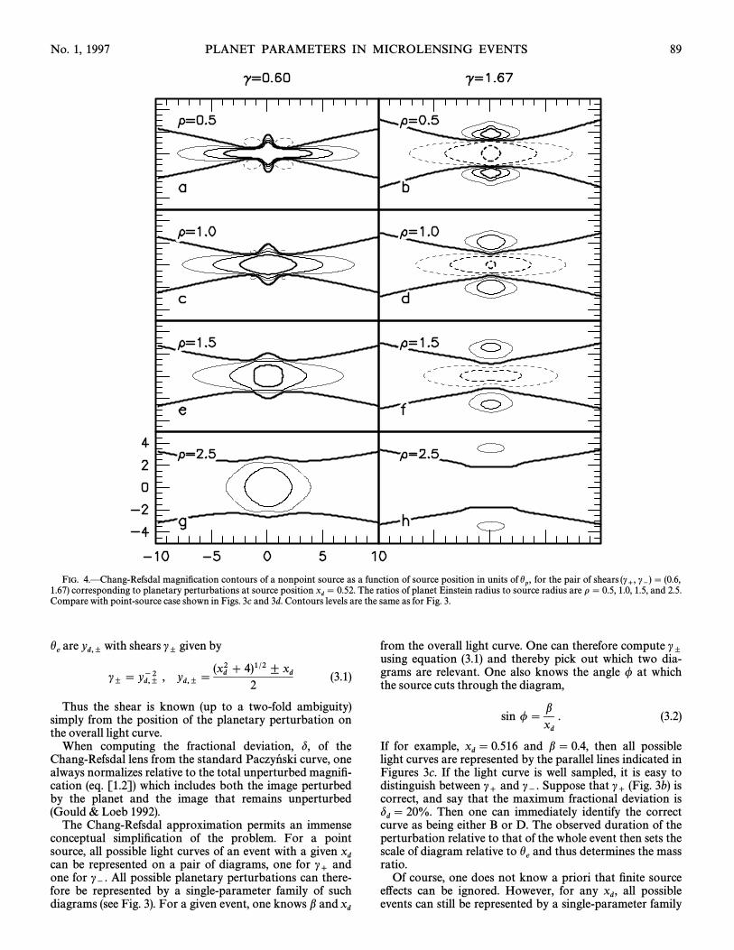
FIG. 4.ÈChang-Refsdal magniÐcation contours of a nonpoint source as a function of source position in units of for the pair of shearshp, (c

`, c~) \ (0.6,

1.67) corresponding to planetary perturbations at source position The ratios of planet Einstein radius to source radius are o \ 0.5, 1.0, 1.5, and 2.5.xd\ 0.52.

Compare with point-source case shown in Figs. and Contours levels are the same as for3c 3d. Fig. 3.

are with shears given byhe

yd,B c

B

cB

\ yd,B~2 , y

d,B\ (xd2 ] 4)1@2 ^ x

d2

(3.1)

Thus the shear is known (up to a two-fold ambiguity)simply from the position of the planetary perturbation onthe overall light curve.

When computing the fractional deviation, d, of theChang-Refsdal lens from the standard Paczyn� ski curve, onealways normalizes relative to the total unperturbed magniÐ-cation which includes both the image perturbed(eq. [1.2])by the planet and the image that remains unperturbed

& Loeb(Gould 1992).The Chang-Refsdal approximation permits an immense

conceptual simpliÐcation of the problem. For a pointsource, all possible light curves of an event with a given x

dcan be represented on a pair of diagrams, one for andc`one for All possible planetary perturbations can there-c~.

fore be represented by a single-parameter family of suchdiagrams (see For a given event, one knows b andFig. 3). x

d

from the overall light curve. One can therefore compute cBusing and thereby pick out which two dia-equation (3.1)

grams are relevant. One also knows the angle / at whichthe source cuts through the diagram,

sin /\ bxd. (3.2)

If for example, and b \ 0.4, then all possiblexd\ 0.516

light curves are represented by the parallel lines indicated inFigures If the light curve is well sampled, it is easy to3c.distinguish between and Suppose that isc

`c~. c

`(Fig. 3b)

correct, and say that the maximum fractional deviation isThen one can immediately identify the correctd

d\ 20%.

curve as being either B or D. The observed duration of theperturbation relative to that of the whole event then sets thescale of diagram relative to and thus determines the massh

eratio.Of course, one does not know a priori that Ðnite source

e†ects can be ignored. However, for any all possiblexd,

events can still be represented by a single-parameter family


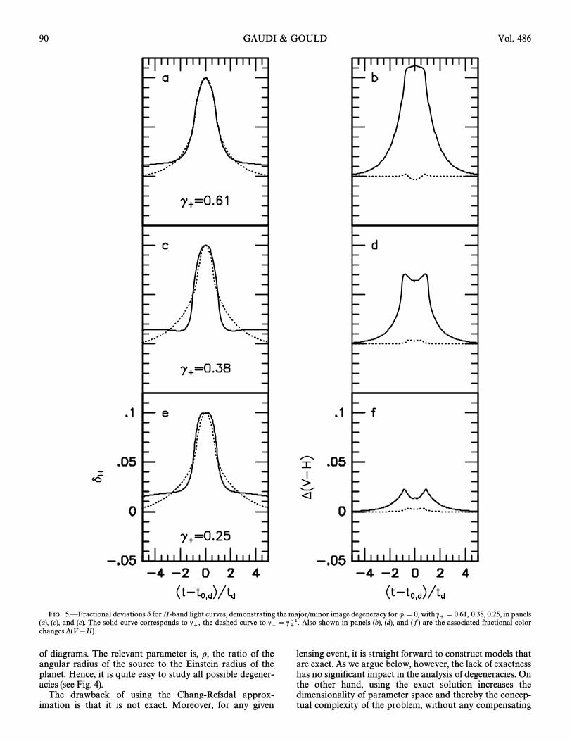
FIG. 5.ÈFractional deviations d for H-band light curves, demonstrating the major/minor image degeneracy for /\ 0, with 0.38, 0.25, in panelsc`

\ 0.61,(a), (c), and (e). The solid curve corresponds to the dashed curve to Also shown in panels (b), (d), and ( f ) are the associated fractional colorc

`, c~ \ c~̀1.

changes *(V [H).

of diagrams. The relevant parameter is, o, the ratio of theangular radius of the source to the Einstein radius of theplanet. Hence, it is quite easy to study all possible degener-acies (see Fig. 4).

The drawback of using the Chang-Refsdal approx-imation is that it is not exact. Moreover, for any given

lensing event, it is straight forward to construct models thatare exact. As we argue below, however, the lack of exactnesshas no signiÐcant impact in the analysis of degeneracies. Onthe other hand, using the exact solution increases thedimensionality of parameter space and thereby the concep-tual complexity of the problem, without any compensating


beneÐts. We therefore strongly advocate using the Chang-Refsdal framework. We present a more detailed analysis inthe Appendix.

4. DEGENERACY BETWEEN MAJOR AND MINOR IMAGES

indicates that it should generally be quite easy toFigure 3distinguish between perturbations of the major image haveone major positive excursion, while perturbations of theminor image have two positive excursions separated by alarge negative excursion. However, if the observations aremade from only one site, then good temporal coverage is farfrom automatic. The timescale for these excursions is theminimum of the crossing time of the star, hr for ah

*/k D 10

giant, and the crossing time of the planet Einstein ringhr. Thus it would be quite possibleh

p/k D 10(m/50 M

^)1@2

to observe a positive excursion (or a signiÐcant fraction ofit) one night and then miss any subsequent excursions dueto one or two nights of bad weather. However, if there werethree observing sites on di†erent continents, such large datagaps would be rare.

There is nevertheless another possible source of degener-acy between the major and minor images. If / is sufficientlysmall, then a source coming close to one of the caustics ofthe perturbations of the minor image could cross the star-planet axis at a point far enough from the planet that thenegative excursion along this axis would be very small. In

panels a, c, and d, we present examples of thisFigure 5,degeneracy for three di†erent values of for /\ 0. Thec

`parameter o was chosen in each case such that the curvesfor and would be most similar. It is clear that thec

`c~degenerate curves could be distinguished only if precise

measurements could be made at the wings of the pertur-bation. We therefore investigate another method of break-ing the degeneracy between the and cases. Followingc

`c~the discussion in if the gradient of the magniÐcation° 1,

across the source is large, and if the surface brightnessproÐle of the source is a function of wavelength, then wewould expect a change in color during the perturbation.This color change depends on the magnitude of the averagegradient across the source is large, i.e., a larger gradientresults in a larger color change. In fact, the gradient of themagniÐcation across the face of the source is much larger inthe case than the case. Measuring the color changec

`c~would therefore enable one to distinguish between the two

cases. Giant stars are more limb-darkened in the opticalthan in the infrared Bell & Gustafsson(Manduca, 1977 ;

and thus lensing of a giant source willManduca 1979),cause a color change. We deÐne the fractional color changeas

*(V [H) \ [2.5 log dV/dH , (4.1)

where V and H are the usual broadband magnitudes, andand are the fractional deviations for V -band andd

VdHH-band respectively. Thus *(V [H) is a measure of di†er-

ence between the lensed and unlensed color (see for a° 6.3more detailed discussion). In panels b, d, and e, weFigure 5,show the fractional color change *(V [H) corresponding tothe perturbations in panels a, c, and d, respectively. Thereare relatively large (2%È10%) fractional color changesassociated with the curves throughout the event, whilec

`the fractional color changes associated with the curvesc~are always negligible. Thus by measuring *(V [H), one candistinguish between the two degenerate cases even during

the peak of the perturbation. The larger the value of /, thelarger the negative excursion in the minor-image pertur-bation, and thus curves with /[ 0 will be less degeneratethan the examples shown in Figure 5.

5. DEGENERACY OF PLANET POSITION RELATION TO

UNPERTURBED IMAGE

Henceforth we will assume that the major/image degener-acy has been broken and the true value of c is known. Thuswe will omit the subscripts ^ from c. Note that values ofc\ 1 refer to major image perturbations and c[ 1 refer tominor image perturbations.

In general, the degeneracy of the planet position relativeto the unperturbed image introduces an uncertainty in y

pwhich is where is the separation between*ypD 2ah

p/h

eah

pthe planet and the unperturbed image at the midpoint of theperturbation. Assume that perturbations of ared

dD 0.05

detectable, and consider only perturbations of the majorimage (c\ 1). As we will show below, this degeneracy is notproblematic for perturbations of the minor image (c[ 1).From one sees that the majority of these pertur-Figure 3bations will be single-peaked, and the peak, will occurd

d,

near the planet-star axis (the x-axes in see, i.e., trajec-Fig. 3 ;tory E). Thus a can be estimated by the point at which thed \ 0.05 contour crosses the planet-star axis. For c\ 0.20,a D 4, whereas for c\ 0.80, a D 14. The range of a will besmaller for any perturbations with The fractionald

d[ 0.05.

uncertainty in is Consideryp\ (c)~1@2 *y

p/y

pD 2a(cq)1@2.

events with cD 0.60. For these events, a D 8 and hence ifthe degeneracy remains unbroken, the fractional error is

For Jupiter-mass planets in orbit*yp/y

pD (150m/M)1@2.

around M dwarfs, this error is of order unity, while forNeptune-mass planets it is D20%. On the other hand, thedegeneracy in q is small (see and alsoTable 1 Appendix).

In this section we consider only point sources. If theplanet has a low mass, so that Ðnite source e†ects areimportant (see and then (as mentioned above)° 1 eq. [1.1]),the di†erence between the two degenerate solutions is smalland distinguishing between them is relatively less impor-tant. In addition, Ðnite-source e†ects are more properlyaddressed in the context of the mass/Ðnite-source degener-acy discussed in ° 6.

5.1. Perturbations of the Major ImageIt is clear from that it is impossible to break theFigure 3

degeneracy if /\ 90¡, i.e., if the planetary perturbationtakes place at the peak of the light curve If the(x

d\b).

source crosses the perturbation structure in the region ofthe caustic then degeneracy is relatively unimpor-(a [ 1)tant and, in any event, is easily broken (provided /\ 90¡)due to the richness of the structure in this region. We there-fore focus on the case a [ 1. From one sees thatFigure 3,there is an asymmetry in the light curve which has oppositesenses depending on whether the source crosses to the leftor the right of the planet. If it passes to the right, then thedeviation is more pronounced at the beginning of the per-turbation than at the end, and if it passes to the left, thedeviation is more pronounced at the end. We deÐne theasymmetry factor as the maximum over all times t of thePÕfractional di†erence,

PÕ(c, dd) 4 max [ o d(t0,d ] t) [ d(t0,d[ t) o ] , (5.1)

where is the midpoint of the perturbation and d(t) is thet0,dfractional deviation as a function of time. To lowest order,


FIG. 6.ÈAsymmetry factor P (see eqs. and for nine values of[5.1] [5.2])c, as a function of maximum deviation, The actual asymmetry of a givend

d.

light curve, is given by Using this ÐgurePÕ(c, dd), PÕ(c, dd

)D P(c, dd) cot /.

and formula, one can therefore determine whether the degeneracy can bebroken for any given sensitivity threshold.

one may approximate

PÕ(c, dd) \ P(c, d

d) cot / . (5.2)

From one can see that as c increases, the positiveFigure 3,contours of d become more stretched along the planet-staraxis, and thus low-peak perturbations occur farther fromthe areas of negative excursion. One would therefore expectsmaller values of P for larger values of c. shows PFigure 6as a function of for several values of c. As expected, Pd

dgenerally decreases with increasing c. Analytically, P(c, isdd)

roughly given by,

P(c, dd) ^G12(1 [ c)d

d,

29(5 [ 12c)dd

,cZ 13 ;c[ 13 .

(5.3)

The break at occurs because the basic structure of thecD 13contours of d changes between c\ 0.40 and c\ 0.20 (seeFor the d [ 0 contours converge to theFig. 3). cZ 13,caustic, whereas for these contours encircle thec[ 0.3,

caustic. This e†ect causes the analytical form of P to exhibita break, and is also reÑected in From orFigure 6. Figure 6,using one can determine, for a given sensi-equation (5.3),tivity, whether the degeneracy can be broken for any pertur-bation. For example, consider trajectories such that /Z

75¡. If one were sensitive to asymmetries of i.e.,PÕD 1%,PD 0.04, then the degeneracy could be broken only for

and then only if On the other hand, ifc[ 0.3, dd[ 0.1.

/D 30¡(PD 0.004), then the degeneracy could be brokenfor essentially all values of c.

5.2. Perturbations of the Minor ImageAs we discussed in to distinguish minor-image from° 4,

major-image perturbations, it is necessary to observe thenegative excursion (centered on the x-axes of the right-handside of If these are observed, then one can easilyFigure 3.distinguish the case where the source transits the right sidefrom the case where it transits the left side of the x-axis

(provided /\ 90¡). Hence, there is no degeneracy of minor-image perturbations unless the more severe major/minor-image degeneracy remains unbroken.

6. CONTINUOUS MASS DEGENERACY OF MAJOR IMAGE

PERTURBATIONS

By far the potentially most crippling form of parameterdegeneracy is the one that is illustrated in and isFigure 2tabulated in The basic character of this degeneracyTable 2.can be understood analytically using the following theorem

& Gaucherel if the unperturbed major image(Gould 1996) :crosses the position of the planet and the source is largerthan the major-image caustic structure, then

dd^

2o2A(c)

, A(c)\ 1 ] c21 [ c2 . (6.1)

The FWHM of such an event is On thetdD 2(csc /)oq1@2t

e.

other hand, the FWHM of a low-peak perturbation of apoint-source is Suppose that a low-peakt

dD 2(csc /)q1@2t

e.

perturbation has observables b, and Now con-te, x

d, t

d, d

d.

sider the combination of observables Q4 [(b/xd)(t

d/te)/2]2.

Then the solution

q D Q , o [ 1 , (6.2)

reproduces the observed values of and However, thedd

td.

solution

q DQ

o'2, o D o' , o'4

A 2dd

1 [ c21 ] c2

B1@2, (6.3)

also reproduces the values of and Note that the ratiodd

td.

of masses for these two solutions is For thiso'2 . ddD 5%,

ratio is typically and can be as high as 40. Thus, unless[20this degeneracy is broken, any low-peak perturbation of apoint source by a Jupiter-mass planet can masquerade as aNeptune-mass event, and vice versa. All intervening massesare permitted as well. Clearly, unless this degeneracy isbroken, low-peak perturbations will contain very littleinformation about mass, and unambiguous detection oflow-mass planets will be impossible. There are three pos-sible paths to breaking this degeneracy.

6.1. Proper-Motion MeasurementIf the proper motion k of the lens relative to the source

were measured, then one could partially break the degener-acy between equations and The angular size of(6.2) (6.3).the source would be known from its dereddened colorh

*and magnitude and StefanÏs law. The time for the source tocross the perturbation x-axis, would thent

cD 2h

*csc //k,

also be known. If one found this would imply thattc\ t

d, t

dwas dominated by the size of the planet Einstein ring, notthe source. Hence, the solution would beequation (6.2),indicated. On the other hand, if one would knowt

cD t

d,

only that the solution was not correct, and that the(6.2)mass ratio lay somewhere in the interval (seeo'~2 Q¹ qQTable 2).

Proper motions can be measured if the lensing star tran-sits or nearly transits the source or by imaging the splitimage of the source using infrared interferometry. See

for a review. Another approach would beGould (1996)simply to wait a few decades and measure the angularseparation of the lens and source. Since typical propermotions are 5 mas yr~1, the separation should be after a0A.1few decades. Unfortunately, most lenses are probably


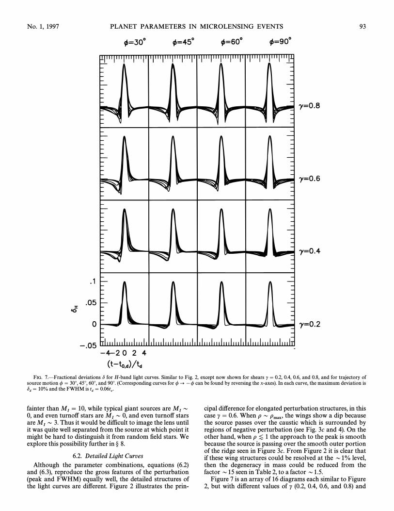
FIG. 7.ÈFractional deviations d for H-band light curves. Similar to except now shown for shears c\ 0.2, 0.4, 0.6, and 0.8, and for trajectory ofFig. 2,source motion /\ 30¡, 45¡, 60¡, and 90¡. (Corresponding curves for /] [/ can be found by reversing the x-axes). In each curve, the maximum deviation is

and the FWHM isdd\ 10% t

d\ 0.06t

e.

fainter than while typical giant sources areMI\ 10, M

ID

0, and even turno† stars are and even turno† starsMID 0,

are Thus it would be difficult to image the lens untilMID 3.

it was quite well separated from the source at which point itmight be hard to distinguish it from random Ðeld stars. Weexplore this possibility further in ° 8.

6.2. Detailed L ight CurvesAlthough the parameter combinations, equations (6.2)

and reproduce the gross features of the perturbation(6.3),(peak and FWHM) equally well, the detailed structures ofthe light curves are di†erent. illustrates the prin-Figure 2

cipal di†erence for elongated perturbation structures, in thiscase c\ 0.6. When the wings show a dip becauseo Do',the source passes over the caustic which is surrounded byregions of negative perturbation (see and On theFig. 3c 4).other hand, when the approach to the peak is smootho [ 1because the source is passing over the smooth outer portionof the ridge seen in From it is clear thatFigure 3c. Figure 2if these wing structures could be resolved at the D1% level,then the degeneracy in mass could be reduced from thefactor D15 seen in to a factor D1.5.Table 2,

is an array of 16 diagrams each similar toFigure 7 Figurebut with di†erent values of c (0.2, 0.4, 0.6, and 0.8) and2,


FIG. 8.ÈValues of (bold lines) and as functions of o for each set of degenerate curves in The Ðducial values and are(q/q0)~1 (k/k0)~1 Fig. 7. q0 k0associated with the curve with o \ 0.1.

di†erent angles of source motion / (30¡, 45¡, 60¡, and 90¡).It is clear that it is easier to break the degeneracy as cincreases and as / decreases. For the uncertainty incZ 0.4q could be signiÐcantly reduced if the wing structures couldbe resolved at the D1% level. For however, dis-c[ 0.2,tinguishing between the degenerate curves would require anaccuracy >1%. shows the values of andFigure 8 q/q0 k/k0as a function of o for each of the combinations of / and c in

Note that larger values of are allowed forFigure 7. o'smaller values of c, and thus the range of acceptable valuesof q is largest for small c. This is especially disturbing inlight of the fact that the degenerate curves are most similarfor small c.

6.3. Optical/Infrared ColorsA major shortcoming of the details light curve method for

breaking the degeneracy is that it depends critically onobtaining accurate observations during two brief intervalscovering the wings of the light curve. As a practical matter,it may be difficult to obtain such coverage for a variety ofreasons. Once the event is noticed, observatories that arededicated to the planet search can engage in frequent moni-toring and thereby obtain very accurate light curves.However, it is quite possible, indeed likely, that the planet-ary perturbation will not be recognized in time for intensivemonitoring of the Ðrst wing. Sometimes observation of the

Ðrst wing is crucial to breaking the degeneracy. Moreover,the second wing will likely be observable from at most oneobservatory which could be a†ected by bad weather.

Optical/infrared color measurements by contrast yielddegeneracy-breaking information throughout the event.The reason is that by the principle of equivalence, lensing ofa point source is achromatic. If lensing introduces colorchanges, the lens must be resolving the source (Witt 1995 ;

& Sasselov The best opportunity to observeLoeb 1995).this e†ect is by looking for optical/infrared color di†erences

& Welch because giant stars are more limb-(Gould 1996)darkened in the optical than in the infrared et al.(Manduca

Thus, if the planet Einstein ring is larger than the1977).source (and the low peak is due to the source passing overregions of small perturbation), the color changes will bevery small. On the other hand, if (and the low peakh

*[ h

poccurs when the large source passes over the caustic), thecaustic structure will resolve the di†erential limb darkeningof the star and the color changes will be more pronounced.We determine the fractional color change using equation

using the limb-darkening model parameterized by the(4.1),surface brightness as a function of angular distance from thecenter of the source,

S(h)S(0)

\ 1 [ i1Y [ i2 Y 2 , Y 4 1 [S

1 [ h2h*2 . (6.4)


FIG. 9.ÈFractional color change *(V [H) for light curves shown in Fig. 7

The coefficients for a cool (4500 K) giant (log g \ 1.5) ofsolar metallicity in V and H are i1V \ 0.798, i2V \ [0.007,

and et al.i1H\ 0.206, i2H\ 0.331 (Manduca 1997 ;See & Welch for further dis-Manduca 1979). Gould (1996)

cussion and their Figure 3 for a graphical representation of[2.5 log shows the V [H colors forS

V(h)/S

H(h). Figure 9

the same parameters as are used for the H-band curves as inThe magnitude of the fractional color change isFigure 7.

largest for smallest c. This is fortunate, since, as discussed inthe degeneracy is most severe for small c, both in° 6.2,

terms of the similarity in the light curves, and in the range ofallowed values of q. It is therefore essential to have optical/

infrared color measurements to ensure that the continuousdegeneracy can be broken for all possible values of c.

7. CONTINUOUS DEGENERACY OF MINOR IMAGE

PERTURBATIONS

There is also a continuous degeneracy for minor-imageperturbations, but the degeneracy is considerably less severethan for major-image perturbations because the causticstructure is qualitatively di†erent. As with major image per-turbations, the basic character of the minor image degener-acy can be understood analytically. Consider the followingtheorem & Gaucherel if the unperturbed(Gould 1996) :


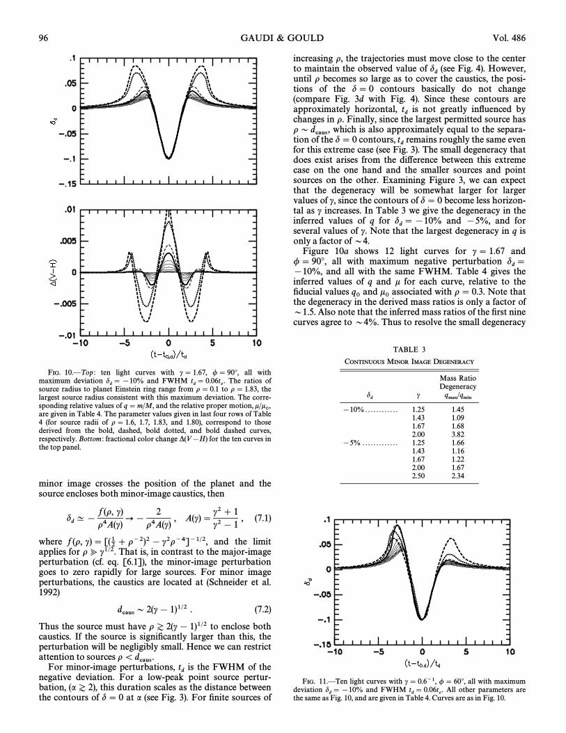
FIG. 10.ÈTop : ten light curves with c\ 1.67, /\ 90¡, all withmaximum deviation and FWHM The ratios ofd

d\ [10% t

d\ 0.06t

e.

source radius to planet Einstein ring range from o \ 0.1 to o \ 1.83, thelargest source radius consistent with this maximum deviation. The corre-sponding relative values of q \ m/M, and the relative proper motion, k/k0,are given in The parameter values given in last four rows of TableTable 4.4 (for source radii of o \ 1.6, 1.7, 1.83, and 1.80), correspond to thosederived from the bold, dashed, bold dotted, and bold dashed curves,respectively. Bottom : fractional color change *(V [H) for the ten curves inthe top panel.

minor image crosses the position of the planet and thesource encloses both minor-image caustics, then

dd^ [ f (o, c)

o4A(c)] [ 2

o4A(c), A(c) \ c2 ] 1

c2 [ 1, (7.1)

where f (o, c) and the limit\ [(12 ] o~2)2 [ c2o~4]~1@2,applies for o ? c1@2. That is, in contrast to the major-imageperturbation (cf. the minor-image perturbationeq. [6.1]),goes to zero rapidly for large sources. For minor imageperturbations, the caustics are located at et al.(Schneider1992)

dcausD 2(c[ 1)1@2 . (7.2)

Thus the source must have to enclose botho Z 2(c [ 1)1@2caustics. If the source is signiÐcantly larger than this, theperturbation will be negligibly small. Hence we can restrictattention to sources o \ dcaus.For minor-image perturbations, is the FWHM of thet

dnegative deviation. For a low-peak point source pertur-bation, this duration scales as the distance between(a Z 2),the contours of d \ 0 at a (see For Ðnite sources ofFig. 3).

increasing o, the trajectories must move close to the centerto maintain the observed value of (see However,d

dFig. 4).

until o becomes so large as to cover the caustics, the posi-tions of the d \ 0 contours basically do not change(compare with Since these contours areFig. 3d Fig. 4).approximately horizontal, is not greatly inÑuenced byt

dchanges in o. Finally, since the largest permitted source haswhich is also approximately equal to the separa-o D dcaus,tion of the d \ 0 contours, remains roughly the same event

dfor this extreme case (see The small degeneracy thatFig. 3).does exist arises from the di†erence between this extremecase on the one hand and the smaller sources and pointsources on the other. Examining we can expectFigure 3,that the degeneracy will be somewhat larger for largervalues of c, since the contours of d \ 0 become less horizon-tal as c increases. In we give the degeneracy in theTable 3inferred values of q for and [5%, and ford

d\[10%

several values of c. Note that the largest degeneracy in q isonly a factor of D4.

shows 12 light curves for c\ 1.67 andFigure 10a/\ 90¡, all with maximum negative perturbation d

d\

[10%, and all with the same FWHM. gives theTable 4inferred values of q and k for each curve, relative to theÐducial values and associated with o \ 0.3. Note thatq0 k0the degeneracy in the derived mass ratios is only a factor ofD1.5. Also note that the inferred mass ratios of the Ðrst ninecurves agree to D4%. Thus to resolve the small degeneracy

TABLE 3

CONTINUOUS MINOR IMAGE DEGENERACY

Mass RatioDegeneracy

dd

c q'/q&[10% . . . . . . . . . . . . 1.25 1.45

1.43 1.091.67 1.682.00 3.82

[5% . . . . . . . . . . . . . 1.25 1.661.43 1.161.67 1.222.00 1.672.50 2.34

FIG. 11.ÈTen light curves with c\ 0.6~1, /\ 60¡, all with maximumdeviation and FWHM All other parameters ared

d\[10% t

d\ 0.06t

e.

the same as and are given in Curves are as inFig. 10, Table 4. Fig. 10.


TABLE 4

DEGENERATE PARAMETER VALUES : CONTINUOUS MINOR IMAGE

Impact Dimensionless Planet/StarParameter Source Radius Mass Ratio Proper Motion

a o q/q0 k/k04.32 . . . . . . . 0.10 0.993 4.0144.30 . . . . . . . 0.20 1.016 1.9844.25 . . . . . . . 0.40 1.000 1.0004.21 . . . . . . . 0.60 1.006 0.6654.00 . . . . . . . 0.80 1.020 0.4953.70 . . . . . . . 1.00 1.033 0.3943.50 . . . . . . . 1.20 1.017 0.3313.20 . . . . . . . 1.40 0.994 0.2872.60 . . . . . . . 1.60 1.004 0.2492.00 . . . . . . . 1.70 1.093 0.2251.00 . . . . . . . 1.83 1.591 0.1730.00 . . . . . . . 1.80 1.628 0.174

in q, one only needs to distinguish between the last fourcurves. From it is clear that this would be pos-Figure 10asible if one could resolve the positive perturbation struc-tures at the D1% level. Furthermore, the situationpresented in for which /\ 90¡, is the worst caseFigure 10,scenario. Due to the structure of the caustics of minor-image perturbations, trajectories with /\ 90¡ displaymarked asymmetry about excepting trajectories witht0,d,a D 0, which are nearly symmetric. This enables one to dis-tinguish between curves with and a D 0 more easilya Z 1when /\ 90¡. This is demonstrated in whichFigure 11,shows 12 light curves with the same parameters as Figure

except that now /\ 60¡. Comparing Figures and10, 10 11,it is clear that the curves are appreciably less degenerate for/\ 60¡ than for /\ 90¡. From we see that theFigure 10b,magnitude of the fractional color change for perturbationswith c\ 1.67 is always small, From*(V [H) [ 1%.numerical calculations, we Ðnd that regard-*(V [H) [ 1%less of the value of c. Thus, in contrast to major imageperturbations, optical/infrared colors are not useful inresolving the degeneracy in minor image perturbationssince the magnitude of the fractional color change is alwayssmall.

8. FROM MASS RATIOS TO PLANET MASSES

If the various degeneracies described in this paper arebroken, one generally recovers two planetary-systemparameters from a planetary microlensing event : q and y

p.

While q is of some interest in its own right, is not. Theypquantities one would most like to know are the planet mass

m\ qM and the physical projected separation ap\ r

eyp.

One could take a purely statistical approach to estimatingthese quantities : given the measured timescale of thet

eevent and a plausible model of the distribution and veloci-ties of lenses and sources along the line of sight, and Mr

ecan be estimated to a factor of 3. In this section, we discusswhat further constraints might be obtained on M and inr

eorder to determine m and ap.

The single most powerful method of acquiring additionalinformation would be to launch a parallax satellite (Refsdal

& Gould which would1966 ; Gould 1995a ; Gaudi 1997)routinely measure and often measure ther8

e4 (Dos/Dls)re

direction of motion as well. This information would, byitself, narrow the uncertainty in the mass to a factor D1.7(see & Gould especially Fig. 7). However, if theHan 1995,proper motion k were also measured, this would yield acomplete solution of the lensing geometry including both Mand (e.g., In general, one expects to measurer

eGould 1996).

k only in D20% of giant events even with relativelyaggressive observations However, for events(Gould 1996).with planetary perturbations, k can be measured muchmore frequently. Recall from that for giant sources,° 6major image perturbations, and planetary masses m[ 100

the planet usually resolves the source (if it is detectedM^

,at all) and that in the process of resolving the resultingdegeneracy, one measures k. Even when the sourceh

*\h

p,

will sometimes cross a caustic in which case k can be mea-sured. Finally, for one can obtain a lower limith

*\ h

pbased on the lack of detection of Ðnite-sourcek [k&e†ects. Since the mass is given by andM \ (c2/4G)r8etek,

since and are measured, this gives a lower limit on ther8e

temass (Gould 1995b).

However, it is much more difficult to resolve the Ðnitesource degeneracy for minor-image perturbations. Eventhough (or rather, because) the measurement of the massratio, q, is not seriously hampered by this degeneracy, theproper motion k is poorly determined (see Thus, it° 2.3.would be necessary to measure k using other methods (see° 6.1).

We now address several questions related to one of thosemethods : direct imaging of the source and lensing starseveral decades after the event. For deÐniteness, we supposethat the measurement is made after 20 years. The expectedseparation is but could plausibly be AtD0A.1, D0A.3.BaadeÏs Window, the expected number of stars MI \ 10inside this radius is D0.5 et al. Thus one(Light 1996).would not be overwhelmed with candidates. On the otherhand, the great majority of lensing events are almost cer-tainly due to objects that are fainter than simplyM

I\ 10

because one does not come close to accounting for theobserved events from the observed stars alone(M

I\ 10)

Thus, to positively identify a candidate star as(Han 1996).the lens, one needs additional information. A parallax satel-lite could provide two pieces of corroborating data. First,the measured together with the proper motion inferredr8

efrom the candidate-source angular separation would give amass and distance to the lens One could(Gould 1995b).then predict an apparent magnitude and see if it agreed withthat of the candidate. Second, if the parallax measurementgave the angle of motion, one could check this against thedirection of the source-candidate separation vector. In addi-tion, the candidateÏs inferred proper motion must satisfy thelower limit derived from lack of Ðnite-source e†ects as dis-cussed above. Finally, one could wait another decade or soto see if the direction of the candidateÏs proper motion wasindeed away from the source. These methods would allowone to unambiguously identify the lens responsible for theevent from the available candidates, thereby enabling one tomeasure k directly.

We would like to to thank the referee, Emilio Falco forhis helpful comments and suggestions. This work was sup-ported in part by grant AST 94-20746 from the NSF, and inpart by grant NAG5-3111 from NASA.


APPENDIX

JUSTIFICATION FOR THE CHANG-REFSDAL APPROXIMATION

What errors are introduced by the Chang-Refsdal approximation? The unperturbed image structure consists of two imagesseparated by greater than The planet, with an e†ective sphere of inÑuence can have a major e†ect on at most2h

e. Dh

p> h

eone of these. For deÐniteness, say this is the major image. In the Chang-Refsdal approximation, the minor image is thentreated as being completely una†ected by the presence of the planet. In fact, the planet will change the shear at the minorimage by and therefore change the magniÐcation by a similar amount. However, what is directly of interest forO(h

p/h

e)

analyzing the planetary perturbation is not the absolute di†erence in magniÐcation with and without the planet. Rather, it isthe change in this di†erence over the lifetime of the planetary perturbation. Hence, the net e†ect is i.e., of higherO[(h

p/h

e)2],

order than the e†ects being analyzed.We now turn to the errors in the Chang-Refsdal estimate of the magniÐcation of the perturbed image. In general, the

perturbed image is split by the planet into two or four images. For each such image, i, the shear due to the parent star is Ifci.

this value were exactly equal to c, the shear at the position of the unperturbed image, then the Chang-Refsdal approximationwould be exact. Typically, is small, so one expects that the errors induced by the approximation*c

i4 c

i[ c *c

i/cDO(h

p/h

e),

are small.We focus Ðrst on perturbations of the major image. Let *h be the separation between the planet and the unperturbed image

and deÐne Consider Ðrst the case a ? 1 which is important when because the magniÐcation contours thena \ *h/hp. cZ 0.5

become signiÐcantly elongated (see The image is then split into two images, one very close to the planet and the otherFig. 3).very close to the unperturbed image. For the image close to the planet, the shear due to the parent star may be signiÐcantlymisestimated, However, for this image, the total shear is dominated by the planet and is O(a2), so true*c

i/cD ah

p/h

e.

fractional error is only Moreover, the magniÐcation of this image is small, O(a~4), so the total error induced byDa~1hp/h

e.

the approximation is and is completely negligible. The other image is displaced by from the unperturbedDa~5hp/h

eDa~1h

pimage, so which induces a similar small change in magniÐcation. Recall from that the source*ci/cD a~1h

p/h

eFigure 3c,

trajectory is determined up to a two-fold degeneracy from the maximum magniÐcation. Since the sign of the image displace-ment is di†erent for the two allowed solutions, the error in estimating the magniÐcation structure could result in two types oferrors. First, there is an error in the planet star separation, but this is only and is therefore lower by a~1 than theDa~1h

pbasic degeneracy indicated in Second, there is an error in the estimate of q and, in fact a degeneracy because theFigure 3c.error has opposite sign for the two allowed solutions. This could in principal be signiÐcant because, within the Chang-Refsdalframework, the two allowed solutions indicated in have identical values of q, and this e†ect is therefore the lowestFigure 3corder degeneracy. However, the mass ratio is estimated from the FWHM of the light curve which is only a weak function ofposition along the elongated magniÐcation contours. Moreover, the misestimate of that position is small. We thereforeestimate a fractional mass degeneracy of *q/q D a~2q1@2.

For and sources that are small compared to the caustic structure (seen e.g., in the situation is similar to that ofa [ 1 Fig. 3),caustic-crossing binary-lens events. The light curves are highly nondegenerate, and one determines not only q and but alsox

p,

o. From the standpoint of understanding degeneracies, the important case is when the source is of order or larger than thecaustic. Here, there are roughly equally magniÐed images displace roughly by on either side of the planet. Hence, the lowesth

porder errors cancel and the next order errors are and can therefore be ignored.DO[hp/h

e)2],

There is one exception to this conclusion. In the argument given above, we implicitly assumed that the planetary pertur-bation would be signiÐcant only over an interval of source motion This assumption fails when the perturbationDh

p.

structure is elongated and when the angle of source motion is low In this case, the local shear is(cZ 0.5) (sin /\ B/xd> 1).

no longer well approximated by the shear at the center of the perturbation. A proper calculation would then require that theshear be recalculated at every point along the source trajectory, holding the planet Ðxed. This was the approach of &GouldLoeb and the resulting magniÐcation for Ðxed planet position can be seen in their Figure 3. (In the present work, by(1992)contrast, what is held Ðxed in constructing Figs. and is the observable : the shear at midpoint of the perturbation). As can3 4be seen by comparing Figure 3c of & Loeb and of the present work, for Jupiter mass planets theGould (1992) Figure 3cdi†erence in contours can be signiÐcant. However, there are three points to note. First, such events are rare both because theconditions together imply and because the elongated contours are encountered ““ edge on,ÏÏ so the(cZ 0.5, b >x

d) b [ 0.2

cross section is only Second, the e†ect is proportional to q1@2 and so would not be signiÐcant for, e.g., Earth-massDhp/h

e.

planets. Third, the nature of the e†ect is to provide information to break degeneracies in cases when the Chang-Refsdalapproximation would lead one to believe that there is no information. In brief, in certain rare cases, the Chang-Refsdalapproximation leads one to underestimate the amount of information available.

For perturbations of the minor image, the two principle sources of degeneracy are Ðrst, confusion of the two caustic peakswith each other and second, confusion of one of these peaks with a perturbation of the major image. Because these peaks areo†set in the direction perpendicular to the star-planet axis, the error in their location is and hence of higher orderO[(h

p/h

e)2]

than their separation. As in the case of the major image, there are certain rare events with sin /> 1 for which theChang-Refsdal approximation makes the degeneracy seem somewhat worse than it is.

REFERENCES

C. 1996, in IAU Symp. 173, Astrophysical Applications of Gravita-Alard,tional Lensing, C. S. Kochanek & J. N. Hewitt (Dordrecht : Kluwer), 214

M., et al. 1996, in IAU Symp. 173, Astrophysical Applications ofAlbrow,Gravitational Lensing, ed. C. S. Kochanek & J. N. Hewitt (Dordrecht :Kluwer), 227

C., et al. 1997, ApJ, 479,Alcock, 119et al. 1996, A&A, 314,Ansari, 94D., & Rhie, H. 1996, ApJ, 472,Bennett, 660A. D., Falco, E. E. 1994, ApJ, 436,Bolatto, 112

K., & Refsdal, S. 1979, Nature, 282,Chang, 561


B. 1997, inGaudi, preparationB., & Gould, A. 1997, ApJ, 477,Gaudi, 152A. 1995a, ApJ, 441,Gould, L211995b, ApJ, 447,ÈÈÈ. 4911996, PAPS, 108,ÈÈÈ. 465A., & Gaucherel, C. 1996, ApJ, 477,Gould, 580A., & Loeb, A. 1992, ApJ, 396,Gould, 104A., & Welch, D. 1996, ApJ, 464,Gould, 212

C. 1997, ApJ, 484,Han, 555C. Gould, A. 1995, ApJ, 447,Han, 53R. M., Baum, W. A., & Holtzman, J. A., 1997, inLight, preparationA., & Sasselov, D. 1995, ApJ, 449,Loeb, 33L

A. 1979, A&AS, 36,Manduca, 411A., Bell, R. A., & Gustafsson, B. 1977, A&A, 61,Manduca, 809

S., & Paczyn� ski, B. 1991, ApJ, 374,Mao, 37B. 1986, ApJ, 304,Paczyn� ski, 1

M. R. et al. 1996, in IAU Symp. 173, Astrophysical Applications ofPratt,Gravitational Lensing, ed. C. S., Kochanek & J. N. Hewitt (Dordrecht :Kluwer), 221

S. 1966, MNRAS, 134,Refsdal, 315P., Ehlers, J., & Falco, E. E. 1992, Gravitational Lenses (Berlin :Schneider,

Springer)A., et al. 1994, Acta Astron., 44,Udalski, 165

H. 1995, ApJ, 449,Witt, 42

Documents

THE ASTROPHYSICAL JOURNAL,486:85È99,1997September1 …