Embed Size (px)
Citation preview
The Astrophysical Journal, 741:115 (20pp), 2011 November 10 doi:10.1088/0004-637X/741/2/115C© 2011. The American Astronomical Society. All rights reserved. Printed in the U.S.A.
THE ASSEMBLY HISTORY OF DISK GALAXIES. I. THE TULLY–FISHER RELATIONTO z � 1.3 FROM DEEP EXPOSURES WITH DEIMOS
Sarah H. Miller1,2, Kevin Bundy3, Mark Sullivan1, Richard S. Ellis2, and Tommaso Treu41 Oxford Astrophysics, Oxford, OX1 3RH, UK; [email protected]
2 California Institute of Technology, Pasadena, CA 91125, USA3 Astronomy Department, University of California, Berkeley, CA 94720, USA
4 UC Santa Barbara Physics, Santa Barbara, CA 93106, USAReceived 2011 February 18; accepted 2011 August 15; published 2011 October 25
ABSTRACT
We present new measures of the evolving scaling relations between stellar mass, luminosity and rotational velocityfor a morphologically inclusive sample of 129 disk-like galaxies with zAB < 22.5 in the redshift range 0.2 < z < 1.3,based on spectra from DEep Imaging Multi-Object Spectrograph on the Keck II telescope, multi-color Hubble SpaceTelescope (HST) Advanced Camera for Surveys photometry, and ground-based Ks-band imaging. A unique featureof our survey is the extended spectroscopic integration times, leading to significant improvements in determiningcharacteristic rotational velocities for each galaxy. Rotation curves are reliably traced to the radius where theybegin to flatten for ∼90% of our sample, and we model the HST-resolved bulge and disk components in orderto accurately de-project our measured velocities, accounting for seeing and dispersion. We demonstrate the meritof these advances by recovering an intrinsic scatter on the stellar mass Tully–Fisher relation a factor of two tothree less than in previous studies at intermediate redshift and comparable to that of locally determined relations.With our increased precision, we find that the relation is well established by 〈z〉 ∼ 1, with no significant evolutionto 〈z〉 ∼ 0.3, ΔM∗ ∼ 0.04 ± 0.07 dex. A clearer trend of evolution is seen in the B-band Tully–Fisher relationcorresponding to a decline in luminosity of ΔMB ∼ 0.85±0.28 magnitudes at fixed velocity over the same redshiftrange, reflecting the changes in star formation over this period. As an illustration of the opportunities possible whengas masses are available for a sample such as ours, we show how our dynamical and stellar mass data can be usedto evaluate the likely contributions of baryons and dark matter to the assembly history of spiral galaxies.
Key words: galaxies: evolution – galaxies: fundamental parameters – galaxies: kinematics and dynamics –galaxies: spiral
Online-only material: color figure, machine-readable table
1. INTRODUCTION
A major challenge for ΛCDM structure formation lies inunderstanding how the baryonic components of galaxies as-semble within dark matter halos. Although baryons representonly one-sixth of the gravitating matter in Wilkinson MicrowaveAnisotropy Probe cosmology (Spergel et al. 2007; Seljak et al.2005), their dissipative properties suggest that they dominatethe inner regions of luminous galaxies (Blumenthal et al. 1986).Determining the interplay between dark matter and baryons iscritical for predicting the evolution of density profiles, substruc-ture, shapes, and angular momentum of galaxies (Governatoet al. 2007; Shlosman 2009). One of the most significant chal-lenges is reproducing the detailed characteristics of rotationallysupported disk galaxies which represent the dominant fractionof present-day luminous systems (Ellis & Silk 2009).
Observational efforts in this challenge have focused on theTully–Fisher (TF) relation (Tully & Fisher 1977) and its pastevolution. This important scaling relation, which correlatesdisk luminosity with rotational velocity, provides an essentialbenchmark for verifying theoretical models based on the stan-dard dark matter picture. Early N-body simulations as well assemi-analytic models produced galaxies that rotate too fast ata given luminosity (van den Bosch 2000; Mo & Mao 2000;Eke et al. 2001; Benson et al. 2003; Dutton et al. 2007).Caused by a transfer of angular momentum from baryons tothe dark matter halo, this deficiency has since been mitigatedby improved resolution, as well as the introduction of feedback(Steinmetz & Navarro 1999), e.g., from supernovae (Governato
et al. 2007; Piontek & Steinmetz 2011). However reproducingthe absolute values observed in the scaling relation has remainedproblematic.
Despite these challenges, the theoretical understanding ofdisk galaxy scaling relations and their evolution has madesome improvement over the past decades. Using an adjustmentto the rotational velocity derived from their hydrodynamicsimulations to account for overmerging, Portinari & Sommer-Larsen (2007) were able to match the observed local TFrelation, and claim a modest evolution to z ∼ 1. Howeverthe predictive power is tempered by an unknown dependenceon redshift of this adjustment. Semi-analytic models have alsoworked to match observations and provide further insight onthe physical interpretation of evolution in the TF relation.Some controversy remains over whether the central regions ofgalaxy halos are subject to adiabatic contraction (Somervilleet al. 2008), broadly maintain a non-evolving density profile(Wechsler et al. 2002), or permit adiabatic expansion (Duttonet al. 2011c). Regardless of the exact evolutionary responseof the inner halo, the persistent picture is one in which thebaryonic component grows in tandem with the dynamical mass(Fall & Efstathiou 1980; Dalcanton et al. 1997; Mo et al. 1998).Gas may cool from the halo or from externally sourced streams,increasing the disk scale length as stars form. In this framework,while any given galaxy is predicted to grow by factors of 1.2–2 instellar mass, dynamical mass, scale radius, and luminosity sincez ∼ 1 (modulo evolutionary corrections), this growth typicallyoccurs along scaling relations, reducing the evolutionary signalsaccessible to observations.
1
The Astrophysical Journal, 741:115 (20pp), 2011 November 10 Miller et al.
Observational progress in testing these pictures of disk as-sembly has been similarly slow. There are significant technicalchallenges in making the necessary measurements at interme-diate redshift and, as a result, there are discrepant conclusionswith regard to evolutionary trends in the literature. In part, thismay reflect different ways in which intermediate-redshift diskgalaxies are selected. Vogt et al. (1996, 1997) undertook animportant pioneering study, finding a modest increase in lumi-nosity (ΔMB ∼ 0.6) at fixed velocity to z ∼ 1, but deduced thisrepresented only an upper limit to possible evolution because ofsample biases and other assumptions. Subsequent optical-basedstudies have presented mixed conclusions. A key uncertainty iswhether to address evolution in the overall mass-to-light ratioindependent of luminosity (i.e., a zero-point shift with redshift)as discussed by Rix et al. (1997), Bamford et al. (2006), andFernandez Lorenzo et al. (2009, 2010), or whether to permitluminosity dependent evolution (i.e., changes in the TF slope)as discussed by Ziegler et al. (2002) and Bohm et al. (2004).TF studies at infrared wavelengths are less affected by biasesinduced by short-term star formation activity and early surveysfound no convincing evolution (Conselice et al. 2005; Floreset al. 2006). However, by contrast, Puech et al. (2008) claimfrom near-IR measures that disks were overall less luminous inthe past. Clearly the rest wavelength at which the luminosity issampled is a key parameter: Fernandez Lorenzo et al. (2010)claim evolution in the B-band but none in redder bands, whileWeiner et al. (2006a, 2006b) find evolution in the slope of theinfrared TF relation consistent with that seen in the blue re-lation; however, they observe little evolution in infrared zeropoint. Moran et al. (2007) have emphasized the importance ofenvironmental influences which can be deduced by consideringthe scatter in the TF relation as a function of local density.
In view of this, a more physically relevant approach forunderstanding the assembly history of disks may be to considerthe stellar mass TF relation (M∗-TF) which, notwithstandingthe difficulty of estimating gas fractions, provides the mostrobust route to understanding the interplay between baryons anddark matter in disk galaxies. Stellar masses are derived usingpopulation model fits to multi-color photometry for galaxiesof known redshift, assuming an initial stellar mass function(Brinchmann & Ellis 2000; Bundy et al. 2005). Although thelow-redshift M∗-TF relation is well constrained (Bell & deJong 2001; Pizagno et al. 2005; Meyer et al. 2008), those atintermediate redshift (Conselice et al. 2005; Flores et al. 2006;Atkinson et al. 2007) reveal a larger scatter than seen in thetraditional TF relations, suggestive of additional uncertainties.A recurrent topic of discussion in the literature is sampleselection and whether evolution seen in both the TF relationand its scatter is driven by redshift-dependent selection criteria.The inclusion of more early types and dynamically disturbedgalaxies likely broadens the intrinsic scatter. In an attempt toinclude more kinematically disturbed galaxies, often excludedwithout good cause in TF studies, Weiner et al. (2006b) andKassin et al. (2007) have included an additional kinematic term,S0.5, which accommodates the isotropic velocity width of theobserved emission lines and reduces the scatter from their classicM∗–rotational-velocity relation. Kassin et al. (2007) detectno significant evolution in the TF relation, including the S0.5relation, over 0.1 < z < 1.2. However, combining a measureof the velocity dispersion with the disk angular momentum mayobscure information about the rotational support of the disk.
Using integral field unit (IFU) spectrographs, Flores et al.(2006) and Puech et al. (2008) have produced intensity, veloc-
ity, and dispersion maps of galaxies at intermediate redshiftsthat demonstrate the unique advantage of a second spatial di-mension in modeling the velocity field and accounting for pro-jection effects. So far, the IFU-based samples are fairly modestin size and sample brighter sources compared to those reachedwith multi-slit techniques. Moreover, the spaxel resolution isoften lower than for the highest-resolution slit spectroscopy.As we will show in this paper, the spectroscopic S/N is anequally important factor in making progress because it deter-mines the radial extent to which emission lines can be tracedand as a result, whether the adopted velocity measure requiresextrapolation.
Both IFUs and slit spectroscopy have been successfully em-ployed at z ≈ 2–3, where near-IR studies can take advantageof redshifted Hα lines—the brightest kinematic tracer—as wellas improved spatial resolution from adaptive optics. Results atthese redshifts may indicate the emergence of regular scalingrelations from more complex and disordered dynamical states.With adequate sampling, at least one-third of z � 2–3 star-forming galaxies show ordered rotation (Shapiro et al. 2008;Stark et al. 2008; Jones et al. 2010) and reveal significantlyhigher velocity dispersions than local counterparts (e.g., Gen-zel et al. 2006). Cresci et al. (2009) have measured the M∗-TFrelation at z ≈ 2 using Spectrograph for INtegral Field Ob-servations in the Near-Infrared (SINFONI) observations of 18rotation-dominated systems in the SINS survey (SpectrographImaging Survey in the Near infrared with SINFONI; ForsterSchreiber et al. 2009). The slope of their measured relation isconsistent with that seen in local observations but offset towardlower M∗ at fixed velocity by ∼0.5 dex. While necessarily bi-ased toward massive systems with well-ordered rotation, thesemay be representative of gas rich systems in transition to z ∼ 1disks (Tacconi et al. 2010). Gnerucci et al. (2011) have recentlymeasured the TF relation at z ∼ 3 from SINFONI IFU data,but because of the large scatter observed, they suggest the TFrelation has not yet been established. However, all points on therelation are consistent with the favored vector of disk assem-bly theory, with a lower average stellar-to-dynamical mass ratiothan found in the local universe.
The present survey was motivated by our desire to chart andunderstand this evolution from a prevalence of disturbed andcomplex dynamical states observed at high z to the well-orderedrotation of local spirals. To make progress, we seek to determinethe M∗-TF relation over the redshift range 0.2 < z < 1.3 withspectroscopic exposures three to eight times that of previousstudies. By including disk systems selected from Hubble SpaceTelescope Advanced Camera for Surveys (HST/ACS) data withirregular or distorted morphologies, we hope to avoid biasesbased on selecting mature, well-ordered disks (Vogt et al. 1996,1997). Our study not only allows us to chart evolution in a largesample down to fainter limits and masses than is possible atz ∼ 2, but the improved precision we demonstrate enables us tomeasure a robust TF relation only a few Gyr later. The scatterwe observe should provide a valuable indication of the rate atwhich disks settle onto the local TF relation. To fully utilizethe gains in S/N ratio from long exposures, we develop animproved method for extracting the rotation curves of galaxiesat intermediate redshift via a new modeling code. While ourresults are based on slit spectroscopy, unlike most previous slit-based studies (Weiner et al. 2006a; Kassin et al. 2007; Bohm &Ziegler 2007), we are able to align the spectral slits on our maskswith the HST-measured major axis, significantly improving thefidelity of our recovered rotation curves at z ∼ 1. We aim to
2
The Astrophysical Journal, 741:115 (20pp), 2011 November 10 Miller et al.
avoid introducing a bias toward aligning the often more extendedand brighter objects at lower redshift over the higher redshiftobjects observed at smaller angular scales, since doing so couldintroduce an extraneous evolution in the offset and scatter of theTF relation with redshift.
The plan of the paper follows. In Section 2, we describeour sample, the Keck spectroscopic data, and the HST/ACSresolved photometry in the north and south Great ObservatoriesOrigins Deep Survey (GOODS) fields. Noting the limitationsof earlier work, Section 3 introduces a new procedure for theanalysis of rotation curve data. We justify our chosen method,discuss error estimation, and compare with previous work. InSection 4 we present the various TF relations, and in Section 5we discuss methods for deriving dynamical masses to compareto baryonic mass estimates for a physical interpretation of ourresults. Finally, Section 6 summarizes the overall conclusionsfor the assembly history of disk galaxies.
Throughout the paper we adopt a Chabrier (2003) ini-tial mass function (IMF) and a ΩΛ = 0.7, Ωm = 0.3,H0 = 70 km s−1 Mpc−1 cosmology. All magnitudes refer tothose in the AB system.
2. DATA
A prerequisite for constructing a disk galaxy sample suitablefor measuring the evolution of the TF relation is deep HST imag-ing essential for morphological selection, resolved photometryand accurate disk position angle data for the multi-slit spectro-scopic campaign. Both northern and southern GOODS fields(Dickinson et al. 2003) are visible from the Keck observatoryand remain the most appropriate areas for such a study given theunique availability of deep multi-color ACS data. In this sectionwe introduce our sample selection criteria (Section 2.1) and thespectroscopic data used for measuring the internal dynamics ofour sample (Section 2.2). We also introduce the photometric dataused for measuring galaxy sizes and shapes (Section 2.3) andstellar mass estimates from spectral energy distribution (SED)fitting (Section 2.4).
2.1. Sample Selection
Our goal in the morphological selection of disk targets is tobe inclusive of all galaxies with disk-like structure, avoiding thetemptation of selecting the most relaxed and “well-behaved”spirals in favor of a more complete census, including the moredisturbed and morphologically abnormal population. Sourceswere selected visually by coauthor R.S.E. from a zF850LP <22.5 sample of 2978 galaxies, in the GOODS North and Southfields, discussed by Bundy et al. (2005). A key differencewith earlier work (i.e., Vogt et al. 1996, 1997; Conseliceet al. 2005) is the inclusion of less mature morphologicaltypes which contain some evidence of disk-like structure, aswell as systems that may be interacting. We included visuallyirregular systems with elongated features, and galaxies withasymmetric and clumpy light distributions. We also includeddisks with dominant bulges. The main aim of broadening themorphological selection criteria was to avoid potential biasesassociated with selecting only symmetric spirals, which mayrepresent the end point of evolution and consequently bias us tolocating mature systems. Within this z-band limited sample, weapplied a further photometric selection, Ks � 22.2, to ensurea high fraction of reliable stellar mass (M∗) estimates to (seeSection 2.4), resulting in a morphologically suitable sampleof 1388 objects. Although spectroscopic redshifts are available
for many of our targets from the Team Keck Redshift Surveyprogram (TKRS; Wirth et al. 2004) in GOODS-N and from theVIMOS-VLT Deep Survey (Le Fevre et al. 2004) in GOODS-S,we did not exclude targets for which only photometric redshiftswere available. Selecting within our target redshift range of0.2 < z < 1.3, we used photometric redshifts from COMBO17(Wolf et al. 2004) and Bundy et al. (2005). As discussed later(Section 3.5), several galaxies within our sample can be foundin earlier kinematic surveys of Flores et al. (2006) and Weineret al. (2006a).
2.2. Spectroscopic Data
Over a number of seasons we collected spectroscopic datafor this sample with the DEIMOS (DEep Imaging Multi-ObjectSpectrograph; Faber et al. 2003) instrument on Keck II. In total,we examined 236 galaxies drawn from the target list discussedin Section 2.1 (17% of total sample), simply chosen to maximizenumber of objects with best position angle alignment with that ofthe mask. Of the 236 spectra, 129 show line emission extendingpast what we will term the “seeing-dispersion beam,”5 59 haveonly very compact emission lines that sample the central region,and 48 are in a category we will refer to as “passive” (meaninggalaxies which show no significant emission lines across thetwo-dimensional (2D) spectrum, although weak lines may berecovered in the integrated spectrum; Figure 1 and Table 1).
The bulk of our analysis is thus based on the 129 galaxieswith extended line emission. While this subsample makes uponly 55% of our initially targeted sample, there is no statisticaldifference in its redshift or apparent magnitude distribution fromthe compact and passive subsets (Figure 1). The only obviousdifferences among the three subsamples concerns their disk sizesand stellar masses. Disks with extended line emission have largerscale radii than those of the compact and passive subsamples,and passive galaxies are largely drawn from the upper end of thetotal stellar mass distribution (see Table 1). These differencesare not surprising and do not lead us to suspect that our workingsample of 129 disk galaxies is significantly biased in its rangeof physical properties compared to the original parent selection.We discuss the properties of our compact emission line sourcesin a later paper in this series.
The DEIMOS observations were undertaken over a seriesof runs from 2004 March through 2008 April. Slit maskswere designed with position angles (P.A.s) within ±30◦ of themeasured P.A. in order to minimize tilt angle corrections in thereduction process. We used the 1200 l mm−1 grating blazed at7500 Å with 1′′ slits (with exception of 7 galaxies observed withthe 600 l mm−1 grating blazed at 7500 Å). In this configuration,we achieved a spectral resolution of 1.7 Å corresponding toa velocity accuracy of 30 km s−1. All DEIMOS data werereduced using the automated spec2d pipeline6 developed by theDEEP2 survey. The spec1d package7 (Davis et al. 2003) wasused to extract one-dimensional (1D) spectra from the rectified2D spectra produced by spec2d. The combination of 1D and 2Dspectra were analyzed using the zspec software, also developedby DEEP2 (Faber et al. 2007; Coil et al. 2004), which fits alinear combination of galaxy, emission line, and stellar templatespectra to each spectrum and allows the user to select the best-fitting template, thus determining the spectroscopic redshift.
5 The seeing-dispersion beam signifies a 2D Gaussian representing thecombination of the effect of seeing along the spatial axis and the emission linevelocity dispersion along the wavelength axis.6 http://astro.berkeley.edu/∼cooper/deep/spec2d/7 Based on http://spectro.princeton.edu/idlspec2d_install.html.
3
The Astrophysical Journal, 741:115 (20pp), 2011 November 10 Miller et al.
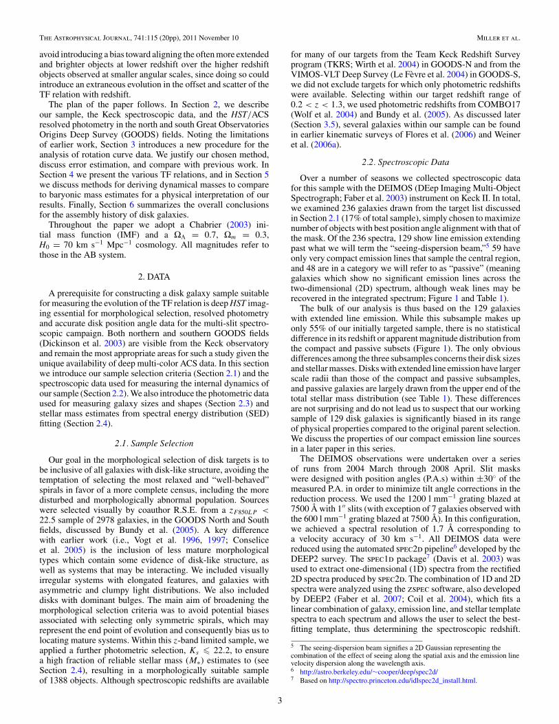
Figure 1. Properties of galaxies in our sample in terms of the distributions of stellar mass estimates, spectroscopic redshifts, zF850LP apparent magnitudes, and diskscale radii. Each histogram is partitioned according to galaxies which have extended emission lines (129), passive spectra with no emission (49) and spectrally compactsources where emission does not extend beyond the central-most regions of their disks (59) (see Section 2.2 and Table 1 for details).
(A color version of this figure is available in the online journal.)
Table 1Disk Sample
Line Profile N 〈log M∗〉a σM∗b 〈rs〉c σrs
d
Extendede 129 10.11 ± 0.05 0.60 2.68 ± 0.09 1.02Compact 59 10.21 ± 0.10 0.73 2.09 ± 0.13 1.01Passive 48 10.69 ± 0.09 0.62 2.24 ± 0.16 1.08
Total 236
Notes. See Figure 1 for histogram and best Gaussian fits of stellar mass andscale radii distribution.a Best-fit Gaussian centroid of log stellar mass.b FWHM of best-fit Gaussian of log stellar mass.c Best-fit Gaussian centroid of scale radii in kpc.d FWHM of best-fit Gaussian of scale radii in kpc.e Possible to fit rotation curves.
This redshift was used as the initial guess for the systematicvelocity in our rotation curve models discussed below.
Because we are interested in the 2D segments of specificemission lines in the spectra, particular care was taken toseparate the reductions of a given mask observed at differenthour angles (and therefore different parallactic angles), taken
on different runs, or observed under varying conditions. Ascheme (discussed below) was developed to coadd 2D spectraof the same target from multiple observation sets prior to furtheranalysis. Because the spatial position of an emission line canvary from one observation to the next as a function of wavelength(by ∼0.′′2), we choose to extract ≈100 Å wavelength “cutouts”around key emission lines of interest (the [O ii] 3727 Å doublet,Hβ, the [O iii] 4959, 5007 Å doublet and Hα) for our rotationcurve study, based on the redshift determined by the zspecanalysis.
Given a set of cutouts for the observation sets of a par-ticular galaxy and emission line, we constructed optimallyweighted coadditions, with weights based on the signal-to-noiseratio (S/N) and seeing FWHM measured from alignment starson the corresponding slit masks. Typically five to six alignmentstars were included on each mask. Relatively sky-free windows(with Δλ � 500 Å) were selected on both the blue and red sidesof each alignment star spectrum. The stellar flux in these win-dows was weighted by the inverse variance (as output from thereduction pipeline) and collapsed along the wavelength direc-tion to obtain a stellar profile fitted with a Gaussian. The widthand peak were used to estimate the S/N and FWHM for the blue
4
The Astrophysical Journal, 741:115 (20pp), 2011 November 10 Miller et al.
and red components of each alignment star. The average FWHMacross a mask and the average star-by-star ratio of S/N valuesprovide the seeing FWHM and relative S/N for that observationset. The typical spread in FWHM among stars on a given maskis 0.′′03. The weight of each observation set was then given byw = s/f 2, where s is S/N and f is the FWHM, and these werenormalized by the weights of all the coadded masks.
All emission line cutouts were inspected by eye and occa-sionally rejected if the region extended beyond the detector areaor if there was an artifact in the data that could interfere with theline of interest. To perform the coaddition, each 2D cutout wasfirst rectified to a regular grid in wavelength and spatial positionusing the 2D wavelength solution output by the spec2d pipeline.We located the peak of the continuum along the spatial axis bycollapsing the 2D cutout in the wavelength direction, initiallymasking out the emission feature. The collapsed profile was fitby a Gaussian with the resulting peak taken as the galaxy center.In rare cases, the continuum was so weak that a position couldnot be determined without including flux from the emission lineitself. The final centering of each cutout was verified by eye,and the cutouts were coadded with appropriate weighting afteralignment in both wavelength and central continuum position.
The seeing varied from 0.′′6 to 1.′′2 over the various observ-ing runs, so whenever seeing measurements are needed in thedynamical analysis (Section 3), we adopt the average value mea-sured from the alignment stars in the final coadded observations.This measurement is preferred to that based on a photometricimage, since it not only refers to data integrated over the entireexposure time of the spectra, but also accounts for systematicsin the observing and coaddition process (which use differentweights for different exposures).
2.3. Photometric Data and Bulge–Disk Decomposition
By selecting our sample within the GOODS North and Southfields, we ensure excellent quality multi-color data for all ourgalaxies from HST/ACS (Giavalisco et al. 2004). This providesvaluable structural information that can be used for translatingthe observed rotation curves into physically based properties. Tothe imaging in four bands from HST (B435, V606, i775, and z850-bands), we add ground-based K-band data in order to securestellar mass estimates based on SED fitting (see Section 2.4).
A key requirement for our analysis is the inclination, P.A. andeffective radius of each galaxy. We also need to separate, wherepossible, the disk light from bulge contamination. We derivethese quantities from the HST imaging using the galfit3 (Peng2010) least-squares elliptical-fitting method. For each galaxywe extracted a 9.′′03 × 9.′′03 (301 × 301 pixels) postage stampcentered on the object. Neighbors were individually maskedout to eliminate confusion. We first fit an exponential diskcomponent plus a de Vaucouleurs’ bulge profile to every galaxy.Those galaxies which yielded unphysical solutions were re-fit with a single Sersic profile component, where the Sersicindex (n) was allowed to vary. Such cases generally representdisk galaxies which are bulgeless and/or more clumpy andirregular than regular well-formed spirals. Approximately 60%of our galaxies were fit using a one-component n-varying Sersicprofile fit, and ∼40% were adequately fit with a two-componentbulge and disk solution. This mixture gives some indicationof the morphological distribution of our sample indicating thatless than half are well-formed spirals (Section 2.1). Disk sizes,inclinations, and P.A.s were taken from best-fit disk componentsif more than one component can be fit. To track possible biases
in the disk–bulge decomposition we will later flag those galaxiesfor which significant bulge components were measured.
We ran galfit using HST data in all four bands (BF435W ,VF606W , iF775W , and zF850LP ). The disk scale radii are consistentamong the bands indicating no significant redshift-dependentbias (or morphological k-correction) within the sample. In or-der to maximize the S/N, hereafter we used the galfit resultsfrom the zF850LP band. To achieve convergence on the galfitparameters and to assess any systematic uncertainty in the fittingtechnique, we ran a Monte Carlo analysis (N = 1000) where wevaried the initial guess of each parameter (magnitude, effectiveradius, b/a for inclination, position angle, and sky) from oneadopted by the GOODS SExtractor results (Giavalisco et al.2004). We found that the parameter output distributions weremuch narrower than the input distributions, thereby demonstrat-ing convergence. Final parameter uncertainties from the MonteCarlo distributions are better than 5% on average, and we addthese uncertainties in quadrature to the observational error.
2.4. Stellar Masses
Reliable stellar masses are an essential component of con-structing a baryonic TF relation. We take our stellar mass es-timates from work initially presented in Bundy et al. (2005),followed by the analysis presented in Bundy et al. (2009). Fur-ther details can be found in those papers.
Briefly, stellar masses are derived using a matched catalog ofmulti-band ACS and ground-based KS photometry. The essentialnear-infrared data was taken with the MOIRCS imager on theSubaru telescope for GOODS-N (Bundy et al. 2009) and theISAAC instrument on the ESO Very Large Telescope (VLT) forGOODS-S (Retzlaff et al. 2010). The final matched catalog issubstantially complete to a limiting magnitude of KAB = 23.8,deeper than our spectroscopic limit.
A Bayesian code fits the SED derived from 2′′ diameter ACSand Ks photometry adopting the best spectroscopic redshiftand this SED is compared to a grid of Bruzual & Charlot(2003) models that span a range of metallicities, star formationhistories, ages and dust content. The stellar mass is estimated bymultiplying the derived K-band mass/light ratio by the observedK-band luminosity derived from the MAG_AUTO total Kronmagnitude determined by SExtractor. We assume a Chabrier(2003) IMF. The probability for each fit is marginalized overthe grid of models giving a stellar mass posterior distributionfunction, the median of which is the catalogued value. At themagnitudes probed in this survey, the uncertainties inferred fromthe width of these posterior functions is less than 0.1 dex.Including systematic errors (see Bundy et al. 2005 for a fulldiscussion), we determine that the stellar masses are reliable tobetter than 0.2 dex, modulo uncertainties arising from the IMFnormalization.
In order to construct a self-consistent TF relation, we applyan aperture correction to the total stellar mass estimates (i.e.,for a given fiducial radius, an aperture stellar mass at that radiuscompared to the velocity measured at that fiducial radius). Weextract equivalent Kron radius aperture fluxes on the zF850LP
band data to get the flux equivalent to that used in the total stellarmass estimates. We then take a scaled-down aperture flux withinthe given fiducial radius, and compare this to the Kron radii flux,thus deriving a total-to-enclosed flux ratio. Assuming that thezF850LP -band and K-band are roughly equivalent stellar tracers,we can use this ratio to estimate the enclosed stellar mass. Thisapproach maximizes the utility of the HST zF850LP images,which have much better resolution than our ground-based
5
The Astrophysical Journal, 741:115 (20pp), 2011 November 10 Miller et al.
K-band data, thereby giving us the resolved mass distributionthroughout the disk to match the detail seen in our rotationcurves.
3. DYNAMICAL ANALYSIS
We now turn to the questions of how to extract reliable rotationcurves from our 2D spectroscopic data and how to interpretthose curves in terms of a fiducial velocity measurement thatcan be used in the various TF relations we will example.To fully exploit our extended integrations, we reexamine therotation curve model and consider carefully how to define a self-consistent fiducial velocity that can be robustly measured withinour data. We quantify improvements in our data by comparingour velocities (extracted from 6–8 hr of integrated exposuretime) with those deduced from ∼1 hr subsets, equivalent toexposures made in previous studies (Vogt et al. 1997; Conseliceet al. 2005; Weiner et al. 2006b; Kassin et al. 2007). Wealso examine the remaining uncertainties given what has beenlearned from the first studies with IFU spectrographs. In whatfollows, our analysis is based on the 129 galaxies for whichextended emission is observed (Section 2.2).
3.1. Rotation Curve Model
Optimally fitting rotation curves presents a variety of chal-lenges that become more difficult as redshift increases. Fore-most, we seek a functional form which represents the bulk ofthe observed emission line shapes and has some physical basis.Second, we must aim to characterize this functional form witha fiducial velocity that is reliably detected across the sample,preferably without extrapolation to radii where there is no data.Given our extended integrations, we have considered carefullythe optimum selection of this characteristic velocity. The chal-lenges can be appreciated by considering Figure 2 where weshow various characteristic velocities in the context of the fre-quently used arctan model of a rotation curve (Courteau 1997)as well as the extent to which we can trace emission lines forour sample.
Several functional forms have been discussed in the literature,such as the “multi-parameter function” in Courteau (1997)and the “universal rotation curve” of Persic et al. (1996). Thesimplest model flexible enough to fit most rotation curves is theempirically motivated arctan function (see Figure 2), which weadopt here, viz:
V = V0 +2
πVa arctan
(r − r0
rt
), (1)
where V0 is the central or systematic velocity, r0 is the dynamiccenter, Va is the asymptotic velocity, and rt is the turnover radius,which is a transitional point between the rising and flatteningpart of the rotation curve (Courteau 1997; Willick 1999). Thearctan model does not account for a sharp peak that is found insome local, bulge-dominated rotation curves around the turnoverradius, but we typically do not observe this feature in our sample.
Past studies employed as TF velocities the maximum mea-sured velocity along the disk, Vmax, or the asymptotic velocityfrom Equation (1), Va (Vogt et al. 1996, 1997; Weiner et al.2006b; Kassin et al. 2007). The disadvantage with Vmax is thatit is not measured at a consistent location in the variety of disksobserved. In terms of the disk scale radius, we can see a rangeof a factor �5 or so in the associated radius.
Some studies (i.e., Flores et al. 2006; Weiner et al. 2006a)advocate the use of Vcirc, the circular radial velocity, driven
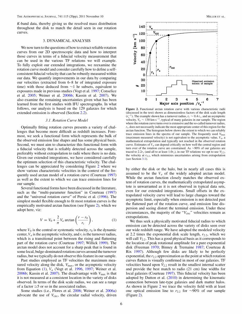
Figure 2. Functional arctan rotation curve with various characteristic radii(discussed in the text) shown as dimensionless factors of the disk scale length(r−1
s ). The example shown has a turnover radius, rt ∼ 0.4 rs , and an asymptoticvelocity, Va ∼ 130 km s−1, typical of many galaxies in our sample. The regionwhere the rotation curve turns over is extensive and the so-called turnover radius,rt , does not necessarily indicate the most appropriate center of this region for thearctan function. The histogram below shows the extent to which we can reliablytrace emission lines in the spectra of our sample. The frequently used Vmax(maximum measured velocity) is not equivalent to the asymptotic value, Va, amathematical extrapolation and typically not reached in the observed rotationcurve. Estimates of Va can depend critically on how well the central region andturn over of the rotation curve are constrained. As ∼90% of our galaxies aretraced to 2.2rs (and all to at least 1.0rs), in our TF relations we opt to use V2.2,the velocity at r2.2, which minimizes uncertainties arising from extrapolation(see Section 3.1).
by either the disk or the halo, but in nearly all cases this isassumed to be the Va of the widely adopted arctan model.While the arctan function closely matches the observed ex-tent of rotation curves, the mathematically extrapolated asymp-tote is unwarranted as it is not observed in typical data sets,even for our extended integrations. Small offsets in the ex-trapolated velocity curve will lead to large changes toward theasymptotic limit, especially when emission is not detected pastthe flattened part of the rotation curve, and emission line dis-persion and seeing distort the terminal emission. Under thesecircumstances, the majority of the “Vcirc” velocities remain asextrapolations.
We thus seek a physically motivated fiducial radius to whichemission can be detected across the variety of disks seen overour wide redshift range. We have adopted the modeled velocityat 2.2 times the exponential disk scale length, r2.2, which wewill call V2.2. This has a good physical basis as it corresponds tothe location of peak rotational amplitude for a pure exponentialdisk (Freeman 1970; Binney & Tremaine 1987; Courteau &Rix 1997). Although few disks are likely to be perfectlyexponential, the r2.2 approximation as the point at which rotationcurves flatten is visually confirmed in most of our galaxies. TFvelocities based upon V2.2 result in the smallest internal scatterand provide the best match to radio (21 cm) line widths forlocal galaxies (Courteau 1997). This fiducial velocity has beenadopted by Dutton et al. (2010) in determining the kinematicconnection between late-type galaxies and dark matter halos.As shown in Figure 2 we trace the velocity field with at leastone optical emission line to r2.2 for ∼90% of our sample(Figure 2).
6
The Astrophysical Journal, 741:115 (20pp), 2011 November 10 Miller et al.
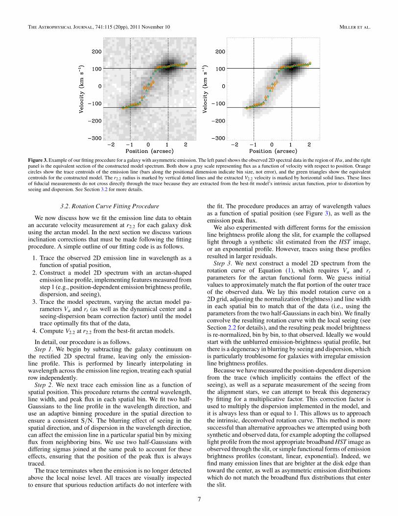
Figure 3. Example of our fitting procedure for a galaxy with asymmetric emission. The left panel shows the observed 2D spectral data in the region of Hα, and the rightpanel is the equivalent section of the constructed model spectrum. Both show a gray scale representing flux as a function of velocity with respect to position. Orangecircles show the trace centroids of the emission line (bars along the positional dimension indicate bin size, not error), and the green triangles show the equivalentcentroids for the constructed model. The r2.2 radius is marked by vertical dotted lines and the extracted V2.2 velocity is marked by horizontal solid lines. These linesof fiducial measurements do not cross directly through the trace because they are extracted from the best-fit model’s intrinsic arctan function, prior to distortion byseeing and dispersion. See Section 3.2 for more details.
3.2. Rotation Curve Fitting Procedure
We now discuss how we fit the emission line data to obtainan accurate velocity measurement at r2.2 for each galaxy diskusing the arctan model. In the next section we discuss variousinclination corrections that must be made following the fittingprocedure. A simple outline of our fitting code is as follows.
1. Trace the observed 2D emission line in wavelength as afunction of spatial position,
2. Construct a model 2D spectrum with an arctan-shapedemission line profile, implementing features measured fromstep 1 (e.g., position-dependent emission brightness profile,dispersion, and seeing),
3. Trace the model spectrum, varying the arctan model pa-rameters Va and rt (as well as the dynamical center and aseeing-dispersion beam correction factor) until the modeltrace optimally fits that of the data,
4. Compute V2.2 at r2.2 from the best-fit arctan models.
In detail, our procedure is as follows.Step 1. We begin by subtracting the galaxy continuum on
the rectified 2D spectral frame, leaving only the emission-line profile. This is performed by linearly interpolating inwavelength across the emission line region, treating each spatialrow independently.
Step 2. We next trace each emission line as a function ofspatial position. This procedure returns the central wavelength,line width, and peak flux in each spatial bin. We fit two half-Gaussians to the line profile in the wavelength direction, anduse an adaptive binning procedure in the spatial direction toensure a consistent S/N. The blurring effect of seeing in thespatial direction, and of dispersion in the wavelength direction,can affect the emission line in a particular spatial bin by mixingflux from neighboring bins. We use two half-Gaussians withdiffering sigmas joined at the same peak to account for theseeffects, ensuring that the position of the peak flux is alwaystraced.
The trace terminates when the emission is no longer detectedabove the local noise level. All traces are visually inspectedto ensure that spurious reduction artifacts do not interfere with
the fit. The procedure produces an array of wavelength valuesas a function of spatial position (see Figure 3), as well as theemission peak flux.
We also experimented with different forms for the emissionline brightness profile along the slit, for example the collapsedlight through a synthetic slit estimated from the HST image,or an exponential profile. However, traces using these profilesresulted in larger residuals.
Step 3. We next construct a model 2D spectrum from therotation curve of Equation (1), which requires Va and rtparameters for the arctan functional form. We guess initialvalues to approximately match the flat portion of the outer traceof the observed data. We lay this model rotation curve on a2D grid, adjusting the normalization (brightness) and line widthin each spatial bin to match that of the data (i.e., using theparameters from the two half-Gaussians in each bin). We finallyconvolve the resulting rotation curve with the local seeing (seeSection 2.2 for details), and the resulting peak model brightnessis re-normalized, bin by bin, to that observed. Ideally we wouldstart with the unblurred emission-brightness spatial profile, butthere is a degeneracy in blurring by seeing and dispersion, whichis particularly troublesome for galaxies with irregular emissionline brightness profiles.
Because we have measured the position-dependent dispersionfrom the trace (which implicitly contains the effect of theseeing), as well as a separate measurement of the seeing fromthe alignment stars, we can attempt to break this degeneracyby fitting for a multiplicative factor. This correction factor isused to multiply the dispersion implemented in the model, andit is always less than or equal to 1. This allows us to approachthe intrinsic, deconvolved rotation curve. This method is moresuccessful than alternative approaches we attempted using bothsynthetic and observed data, for example adopting the collapsedlight profile from the most appropriate broadband HST image asobserved through the slit, or simple functional forms of emissionbrightness profiles (constant, linear, exponential). Indeed, wefind many emission lines that are brighter at the disk edge thantoward the center, as well as asymmetric emission distributionswhich do not match the broadband flux distributions that enterthe slit.
7
The Astrophysical Journal, 741:115 (20pp), 2011 November 10 Miller et al.
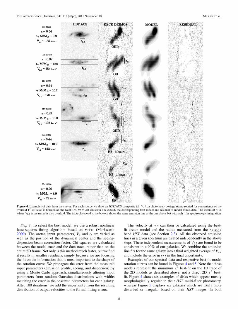
Figure 4. Examples of data from the survey. For each source we show an HST/ACS composite (B, V, i, z) photometry postage stamp rotated for convenience so theoverlaid 1′′ slit level is horizontal, the Keck DEIMOS 2D emission line cutout, the corresponding best model and residual of model minus data. The extent of r2.2,where V2.2 is measured is also overlaid. The triptych second to the bottom shows the same emission line as the one above but with only 1 hr spectroscopic integration.
Step 4. To select the best model, we use a robust nonlinearleast-squares fitting algorithm based on mpfit (Markwardt2009). The arctan input parameters, Va and rt are varied aswell as the position of the dynamical center and the seeing-dispersion beam correction factor. Chi-squares are calculatedbetween the model trace and the data trace, rather than on theentire 2D frame. Not only is this method much faster, but we findit results in smaller residuals, simply because we are focusingthe fit on the information that is most important to the shape ofthe rotation curve. We propagate the error from the measuredinput parameters (emission profile, seeing, and dispersion) byusing a Monte Carlo approach, simultaneously altering inputparameters from random Gaussian distributions with widthsmatching the error in the observed parameters for each galaxy.After 100 iterations, we add the uncertainty from the resultingdistribution of output velocities to the formal fitting errors.
The velocity at r2.2 can then be calculated using the best-fit arctan model and the radius measured from the zF850LP
band HST data (see Section 2.3). All the observed emissionlines in a given spectrum are treated independently in the abovesteps. These independent measurements of V2.2 are found to beconsistent in >90% of our galaxies. We combine the emissionline fits for the same galaxy into a final weighted average of V2.2and include the error in r2.2 in the final uncertainty.
Examples of our spectral data and respective best-fit modelrotation curves can be found in Figures 4 and 5. Note that thesemodels represent the minimum χ2 best-fit on the 1D trace ofthe 2D models as described above, not a direct 2D χ2 best-fit. Figure 4 shows six examples of disks which appear mostlymorphologically regular in their HST multi-filter photometry,whereas Figure 5 displays six galaxies which are likely moredisturbed or irregular based on their HST images. In both
8

The Astrophysical Journal, 741:115 (20pp), 2011 November 10 Miller et al.
Figure 5. As Figure 4 but for more disturbed, visually asymmetric disks, some of which appear to be undergoing minor mergers. Although the morphologies are moreirregular, we usually succeed in fitting an appropriate arctan-based model.
figure sets, we observe fairly regular arctan-shaped kinematics,although places of high dispersion and brightness in the emissionline tend to coincide with regions of the galaxy in the HST imagethat appear to be internally or externally disturbed. For the fifthgalaxy in both figures, we show the best-fit model rotation curveafter only 1 hr of integration time for a comparison to the full6–8 hr of integration shown in the panel just above.
3.3. Inclination and P.A. Offset Corrections
We now correct our V2.2 measurements for the effects ofdisk inclination and any misalignment between the P.A. of theDEIMOS slit and the major axis of the galaxy as determinedfrom galfit.
Adopting the convention i = 0◦ for face-on and i = 90◦ foredge-on disks, the inclination correction is
Vcorr = Vobs
(sin i), (2)
i = cos−1
√(b/a)2 − q2
0
1 − q20
, (3)
where q0 � 0.1–0.2 represents the intrinsic flattening ratioof an edge-on galaxy (Haynes & Giovanelli 1984; Courteau1996; Tully et al. 1998). Although the precise value dependson morphology, the uncertainty leads to changes in the finalvelocity measurement on the order of 1 km s−1 (Pizagno et al.2005; Haynes & Giovanelli 1984). We assumed q0 = 0.19 forall systems, similar to Pizagno et al. (2005).
9
The Astrophysical Journal, 741:115 (20pp), 2011 November 10 Miller et al.
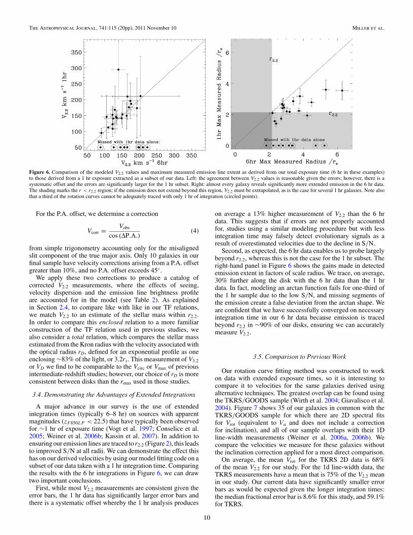
Figure 6. Comparison of the modeled V2.2 values and maximum measured emission line extent as derived from our total exposure time (6 hr in these examples)to those derived from a 1 hr exposure extracted as a subset of our data. Left: the agreement between V2.2 values is reasonable given the errors; however, there is asystematic offset and the errors are significantly larger for the 1 hr subset. Right: almost every galaxy reveals significantly more extended emission in the 6 hr data.The shading marks the r < r2.2 region; if the emission does not extend beyond this region, V2.2 must be extrapolated, as is the case for several 1 hr galaxies. Note alsothat a third of the rotation curves cannot be adequately traced with only 1 hr of integration (circled points).
For the P.A. offset, we determine a correction
Vcorr = Vobs
cos (ΔP.A.)(4)
from simple trigonometry accounting only for the misalignedslit component of the true major axis. Only 10 galaxies in ourfinal sample have velocity corrections arising from a P.A. offsetgreater than 10%, and no P.A. offset exceeds 45◦.
We apply these two corrections to produce a catalog ofcorrected V2.2 measurements, where the effects of seeing,velocity dispersion and the emission line brightness profileare accounted for in the model (see Table 2). As explainedin Section 2.4, to compare like with like in our TF relations,we match V2.2 to an estimate of the stellar mass within r2.2.In order to compare this enclosed relation to a more familiarconstruction of the TF relation used in previous studies, wealso consider a total relation, which compares the stellar massestimated from the Kron radius with the velocity associated withthe optical radius rD, defined for an exponential profile as oneenclosing ∼83% of the light, or 3.2rs. This measurement of V3.2or VD we find to be comparable to the Vcirc or Vmax of previousintermediate-redshift studies; however, our choice of rD is moreconsistent between disks than the rmax used in those studies.
3.4. Demonstrating the Advantages of Extended Integrations
A major advance in our survey is the use of extendedintegration times (typically 6–8 hr) on sources with apparentmagnitudes (zF850LP < 22.5) that have typically been observedfor ∼1 hr of exposure time (Vogt et al. 1997; Conselice et al.2005; Weiner et al. 2006b; Kassin et al. 2007). In addition toensuring our emission lines are traced to r2.2 (Figure 2), this leadsto improved S/N at all radii. We can demonstrate the effect thishas on our derived velocities by using our model fitting code on asubset of our data taken with a 1 hr integration time. Comparingthe results with the 6 hr integrations in Figure 6, we can drawtwo important conclusions.
First, while most V2.2 measurements are consistent given theerror bars, the 1 hr data has significantly larger error bars andthere is a systematic offset whereby the 1 hr analysis produces
on average a 13% higher measurement of V2.2 than the 6 hrdata. This suggests that if errors are not properly accountedfor, studies using a similar modeling procedure but with lessintegration time may falsely detect evolutionary signals as aresult of overestimated velocities due to the decline in S/N.
Second, as expected, the 6 hr data enables us to probe largelybeyond r2.2, whereas this is not the case for the 1 hr subset. Theright-hand panel in Figure 6 shows the gains made in detectedemission extent in factors of scale radius. We trace, on average,30% further along the disk with the 6 hr data than the 1 hrdata. In fact, modeling an arctan function fails for one-third ofthe 1 hr sample due to the low S/N, and missing segments ofthe emission create a false deviation from the arctan shape. Weare confident that we have successfully converged on necessaryintegration time in our 6 hr data because emission is tracedbeyond r2.2 in ∼90% of our disks, ensuring we can accuratelymeasure V2.2.
3.5. Comparison to Previous Work
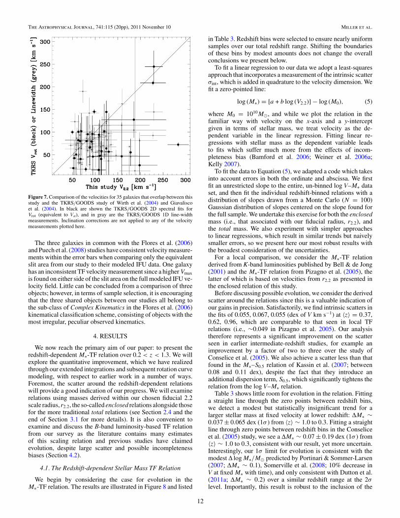
Our rotation curve fitting method was constructed to workon data with extended exposure times, so it is interesting tocompare it to velocities for the same galaxies derived usingalternative techniques. The greatest overlap can be found usingthe TKRS/GOODS sample (Wirth et al. 2004; Giavalisco et al.2004). Figure 7 shows 35 of our galaxies in common with theTKRS/GOODS sample for which there are 2D spectral fitsfor Vrot (equivalent to Va and does not include a correctionfor inclination), and all of our sample overlaps with their 1Dline-width measurements (Weiner et al. 2006a, 2006b). Wecompare the velocities we measure for these galaxies withoutthe inclination correction applied for a most direct comparison.
On average, the mean Vrot for the TKRS 2D data is 68%of the mean V2.2 for our study. For the 1d line-width data, theTKRS measurements have a mean that is 75% of the V2.2 meanin our study. Our current data have significantly smaller errorbars as would be expected given the longer integration times:the median fractional error bar is 8.6% for this study, and 59.1%for TKRS.
10
Th
eA
strophysical
Journ
al,741:115(20pp),2011
Novem
ber10
Miller
etal.
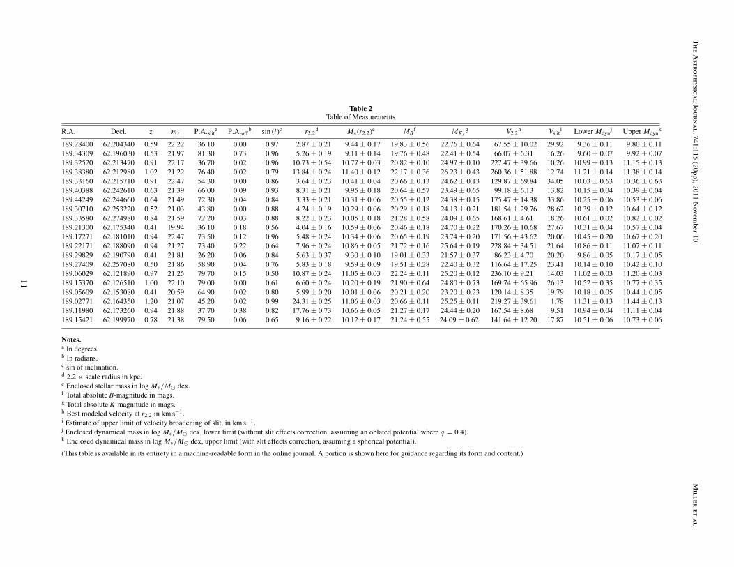
Table 2Table of Measurements
R.A. Decl. z mz P.A.slita P.A.off
b sin (i)c r2.2d M∗(r2.2)e MB
f MKsg V2.2
h Vsliti Lower Mdyn
j Upper Mdynk
189.28400 62.204340 0.59 22.22 36.10 0.00 0.97 2.87 ± 0.21 9.44 ± 0.17 19.83 ± 0.56 22.76 ± 0.64 67.55 ± 10.02 29.92 9.36 ± 0.11 9.80 ± 0.11189.34309 62.196030 0.53 21.97 81.30 0.73 0.96 5.26 ± 0.19 9.11 ± 0.14 19.76 ± 0.48 22.41 ± 0.54 66.07 ± 6.31 16.26 9.60 ± 0.07 9.92 ± 0.07189.32520 62.213470 0.91 22.17 36.70 0.02 0.96 10.73 ± 0.54 10.77 ± 0.03 20.82 ± 0.10 24.97 ± 0.10 227.47 ± 39.66 10.26 10.99 ± 0.13 11.15 ± 0.13189.38380 62.212980 1.02 21.22 76.40 0.02 0.79 13.84 ± 0.24 11.40 ± 0.12 22.17 ± 0.36 26.23 ± 0.43 260.36 ± 51.88 12.74 11.21 ± 0.14 11.38 ± 0.14189.33160 62.215710 0.91 22.47 54.30 0.00 0.86 3.64 ± 0.23 10.41 ± 0.04 20.66 ± 0.13 24.62 ± 0.13 129.87 ± 69.84 34.05 10.03 ± 0.63 10.36 ± 0.63189.40388 62.242610 0.63 21.39 66.00 0.09 0.93 8.31 ± 0.21 9.95 ± 0.18 20.64 ± 0.57 23.49 ± 0.65 99.18 ± 6.13 13.82 10.15 ± 0.04 10.39 ± 0.04189.44249 62.244660 0.64 21.49 72.30 0.04 0.84 3.33 ± 0.21 10.31 ± 0.06 20.55 ± 0.12 24.38 ± 0.15 175.47 ± 14.38 33.86 10.25 ± 0.06 10.53 ± 0.06189.30710 62.253220 0.52 21.03 43.80 0.00 0.88 4.24 ± 0.19 10.29 ± 0.06 20.29 ± 0.18 24.13 ± 0.21 181.54 ± 29.76 28.62 10.39 ± 0.12 10.64 ± 0.12189.33580 62.274980 0.84 21.59 72.20 0.03 0.88 8.22 ± 0.23 10.05 ± 0.18 21.28 ± 0.58 24.09 ± 0.65 168.61 ± 4.61 18.26 10.61 ± 0.02 10.82 ± 0.02189.21300 62.175340 0.41 19.94 36.10 0.18 0.56 4.04 ± 0.16 10.59 ± 0.06 20.46 ± 0.18 24.70 ± 0.22 170.26 ± 10.68 27.67 10.31 ± 0.04 10.57 ± 0.04189.17271 62.181010 0.94 22.47 73.50 0.12 0.96 5.48 ± 0.24 10.34 ± 0.06 20.65 ± 0.19 23.74 ± 0.20 171.56 ± 43.62 20.06 10.45 ± 0.20 10.67 ± 0.20189.22171 62.188090 0.94 21.27 73.40 0.22 0.64 7.96 ± 0.24 10.86 ± 0.05 21.72 ± 0.16 25.64 ± 0.19 228.84 ± 34.51 21.64 10.86 ± 0.11 11.07 ± 0.11189.29829 62.190790 0.41 21.81 26.20 0.06 0.84 5.63 ± 0.37 9.30 ± 0.10 19.01 ± 0.33 21.57 ± 0.37 86.23 ± 4.70 20.20 9.86 ± 0.05 10.17 ± 0.05189.27409 62.257080 0.50 21.86 58.90 0.04 0.76 5.83 ± 0.18 9.59 ± 0.09 19.51 ± 0.28 22.40 ± 0.32 116.64 ± 17.25 23.41 10.14 ± 0.10 10.42 ± 0.10189.06029 62.121890 0.97 21.25 79.70 0.15 0.50 10.87 ± 0.24 11.05 ± 0.03 22.24 ± 0.11 25.20 ± 0.12 236.10 ± 9.21 14.03 11.02 ± 0.03 11.20 ± 0.03189.15370 62.126510 1.00 22.10 79.00 0.00 0.61 6.60 ± 0.24 10.20 ± 0.19 21.90 ± 0.64 24.80 ± 0.73 169.74 ± 65.96 26.13 10.52 ± 0.35 10.77 ± 0.35189.05609 62.153080 0.41 20.59 64.90 0.02 0.80 5.99 ± 0.20 10.01 ± 0.06 20.21 ± 0.20 23.20 ± 0.23 120.14 ± 8.35 19.79 10.18 ± 0.05 10.44 ± 0.05189.02771 62.164350 1.20 21.07 45.20 0.02 0.99 24.31 ± 0.25 11.06 ± 0.03 20.66 ± 0.11 25.25 ± 0.11 219.27 ± 39.61 1.78 11.31 ± 0.13 11.44 ± 0.13189.11980 62.173260 0.94 21.88 37.70 0.38 0.82 17.76 ± 0.73 10.66 ± 0.05 21.27 ± 0.17 24.44 ± 0.20 167.54 ± 8.68 9.51 10.94 ± 0.04 11.11 ± 0.04189.15421 62.199970 0.78 21.38 79.50 0.06 0.65 9.16 ± 0.22 10.12 ± 0.17 21.24 ± 0.55 24.09 ± 0.62 141.64 ± 12.20 17.87 10.51 ± 0.06 10.73 ± 0.06
Notes.a In degrees.b In radians.c sin of inclination.d 2.2 × scale radius in kpc.e Enclosed stellar mass in log M∗/M� dex.f Total absolute B-magnitude in mags.g Total absolute K-magnitude in mags.h Best modeled velocity at r2.2 in km s−1.i Estimate of upper limit of velocity broadening of slit, in km s−1.j Enclosed dynamical mass in log M∗/M� dex, lower limit (without slit effects correction, assuming an oblated potential where q = 0.4).k Enclosed dynamical mass in log M∗/M� dex, upper limit (with slit effects correction, assuming a spherical potential).
(This table is available in its entirety in a machine-readable form in the online journal. A portion is shown here for guidance regarding its form and content.)
11
The Astrophysical Journal, 741:115 (20pp), 2011 November 10 Miller et al.
Figure 7. Comparison of the velocities for 35 galaxies that overlap between thisstudy and the TKRS/GOODS study of Wirth et al. (2004) and Giavaliscoet al. (2004). In black are shown the TKRS/GOODS 2D spectral fits forVrot (equivalent to Va), and in gray are the TKRS/GOODS 1D line-widthmeasurements. Inclination corrections are not applied to any of the velocitymeasurements plotted here.
The three galaxies in common with the Flores et al. (2006)and Puech et al. (2008) studies have consistent velocity measure-ments within the error bars when comparing only the equivalentslit area from our study to their modeled IFU data. One galaxyhas an inconsistent TF velocity measurement since a higher Vmaxis found on either side of the slit area on the full modeled IFU ve-locity field. Little can be concluded from a comparison of threeobjects; however, in terms of sample selection, it is encouragingthat the three shared objects between our studies all belong tothe sub-class of Complex Kinematics in the Flores et al. (2006)kinematical classification scheme, consisting of objects with themost irregular, peculiar observed kinematics.
4. RESULTS
We now reach the primary aim of our paper: to present theredshift-dependent M∗-TF relation over 0.2 < z < 1.3. We willexplore the quantitative improvement, which we have realizedthrough our extended integrations and subsequent rotation curvemodeling, with respect to earlier work in a number of ways.Foremost, the scatter around the redshift-dependent relationswill provide a good indication of our progress. We will examinerelations using masses derived within our chosen fiducial 2.2scale radius, r2.2, the so-called enclosed relations alongside thosefor the more traditional total relations (see Section 2.4 and theend of Section 3.1 for more details). It is also convenient toexamine and discuss the B-band luminosity-based TF relationfrom our survey as the literature contains many estimatesof this scaling relation and previous studies have claimedevolution, despite large scatter and possible incompletenessbiases (Section 4.2).
4.1. The Redshift-dependent Stellar Mass TF Relation
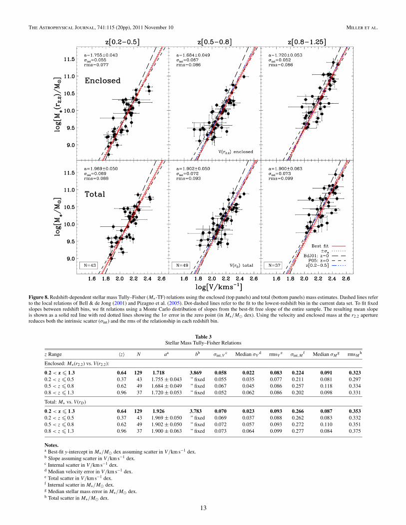
We begin by considering the case for evolution in theM∗-TF relation. The results are illustrated in Figure 8 and listed
in Table 3. Redshift bins were selected to ensure nearly uniformsamples over our total redshift range. Shifting the boundariesof these bins by modest amounts does not change the overallconclusions we present below.
To fit a linear regression to our data we adopt a least-squaresapproach that incorporates a measurement of the intrinsic scatterσint, which is added in quadrature to the velocity dimension. Wefit a zero-pointed line:
log (M∗) = [a + b log (V2.2)] − log (M0), (5)
where M0 = 1010M�, and while we plot the relation in thefamiliar way with velocity on the x-axis and a y-interceptgiven in terms of stellar mass, we treat velocity as the de-pendent variable in the linear regression. Fitting linear re-gressions with stellar mass as the dependent variable leadsto fits which suffer much more from the effects of incom-pleteness bias (Bamford et al. 2006; Weiner et al. 2006a;Kelly 2007).
To fit the data to Equation (5), we adapted a code which takesinto account errors in both the ordinate and abscissa. We firstfit an unrestricted slope to the entire, un-binned log V–M∗ dataset, and then fit the individual redshift-binned relations with adistribution of slopes drawn from a Monte Carlo (N = 100)Gaussian distribution of slopes centered on the slope found forthe full sample. We undertake this exercise for both the enclosedmass (i.e., that associated with our fiducial radius, r2.2), andthe total mass. We also experiment with simpler approachesto linear regressions, which result in similar trends but naivelysmaller errors, so we present here our most robust results withthe broadest consideration of the uncertainties.
For a local comparison, we consider the M∗-TF relationderived from K-band luminosities published by Bell & de Jong(2001) and the M∗-TF relation from Pizagno et al. (2005), thelatter of which is based on velocities from r2.2 as presented inthe enclosed relation of this study.
Before discussing possible evolution, we consider the derivedscatter around the relations since this is a valuable indication ofour gains in precision. Satisfactorily, we find intrinsic scatters inthe fits of 0.055, 0.067, 0.055 (dex of V km s−1) at 〈z〉 = 0.37,0.62, 0.96, which are comparable to that seen in local TFrelations (i.e., ∼0.049 in Pizagno et al. 2005). Our analysistherefore represents a significant improvement on the scatterseen in earlier intermediate-redshift studies, for example animprovement by a factor of two to three over the study ofConselice et al. (2005). We also achieve a scatter less than thatfound in the M∗–S0.5 relation of Kassin et al. (2007; between0.08 and 0.11 dex), despite the fact that they introduce anadditional dispersion term, S0.5, which significantly tightens therelation from the log V–M∗ relation.
Table 3 shows little room for evolution in the relation. Fittinga straight line through the zero points between redshift bins,we detect a modest but statistically insignificant trend for alarger stellar mass at fixed velocity at lower redshift: ΔM∗ ∼0.037 ± 0.065 dex (1σ ) from 〈z〉 ∼ 1.0 to 0.3. Fitting a straightline through zero points between redshift bins in the Conseliceet al. (2005) study, we see a ΔM∗ ∼ 0.07 ± 0.19 dex (1σ ) from〈z〉 ∼ 1.0 to 0.3, consistent with our result, yet more uncertain.Interestingly, our 1σ limit for evolution is consistent with themodest Δ log M∗/M� predicted by Portinari & Sommer-Larsen(2007; ΔM∗ ∼ 0.1), Somerville et al. (2008; 10% decrease inV at fixed M∗ with time), and only consistent with Dutton et al.(2011a; ΔM∗ ∼ 0.2) over a similar redshift range at the 2σlevel. Importantly, this result is robust to the inclusion of the
12
The Astrophysical Journal, 741:115 (20pp), 2011 November 10 Miller et al.
Figure 8. Redshift-dependent stellar mass Tully–Fisher (M∗-TF) relations using the enclosed (top panels) and total (bottom panels) mass estimates. Dashed lines referto the local relations of Bell & de Jong (2001) and Pizagno et al. (2005). Dot-dashed lines refer to the fit to the lowest-redshift bin in the current data set. To fit fixedslopes between redshift bins, we fit relations using a Monte Carlo distribution of slopes from the best-fit free slope of the entire sample. The resulting mean slopeis shown as a solid red line with red dotted lines showing the 1σ error in the zero point (in M∗/M� dex). Using the velocity and enclosed mass at the r2.2 aperturereduces both the intrinsic scatter (σint) and the rms of the relationship in each redshift bin.
Table 3Stellar Mass Tully–Fisher Relations
z Range 〈z〉 N aa bb σint,Vc Median σV
d rmsVe σint,M
f Median σMg rmsM
h
Enclosed: M∗(r2.2) vs. V(r2.2):
0.2 < z � 1.3 0.64 129 1.718 3.869 0.058 0.022 0.083 0.224 0.091 0.3230.2 < z � 0.5 0.37 43 1.755 ± 0.043 ” fixed 0.055 0.035 0.077 0.211 0.081 0.2970.5 < z � 0.8 0.62 49 1.684 ± 0.049 ” fixed 0.067 0.045 0.086 0.257 0.118 0.3340.8 < z � 1.3 0.96 37 1.720 ± 0.053 ” fixed 0.052 0.062 0.086 0.202 0.098 0.331
Total: M∗ vs. V(rD)
0.2 < z � 1.3 0.64 129 1.926 3.783 0.070 0.023 0.093 0.266 0.087 0.3530.2 < z � 0.5 0.37 43 1.969 ± 0.050 ” fixed 0.069 0.037 0.088 0.262 0.083 0.3320.5 < z � 0.8 0.62 49 1.902 ± 0.050 ” fixed 0.072 0.057 0.093 0.272 0.110 0.3510.8 < z � 1.3 0.96 37 1.900 ± 0.063 ” fixed 0.073 0.064 0.099 0.277 0.084 0.375
Notes.a Best-fit y-intercept in M∗/M� dex assuming scatter in V/km s−1 dex.b Slope assuming scatter in V/km s−1 dex.c Internal scatter in V/km s−1 dex.d Median velocity error in V/km s−1 dex.e Total scatter in V/km s−1 dex.f Internal scatter in M∗/M� dex.g Median stellar mass error in M∗/M� dex.h Total scatter in M∗/M� dex.
13
The Astrophysical Journal, 741:115 (20pp), 2011 November 10 Miller et al.
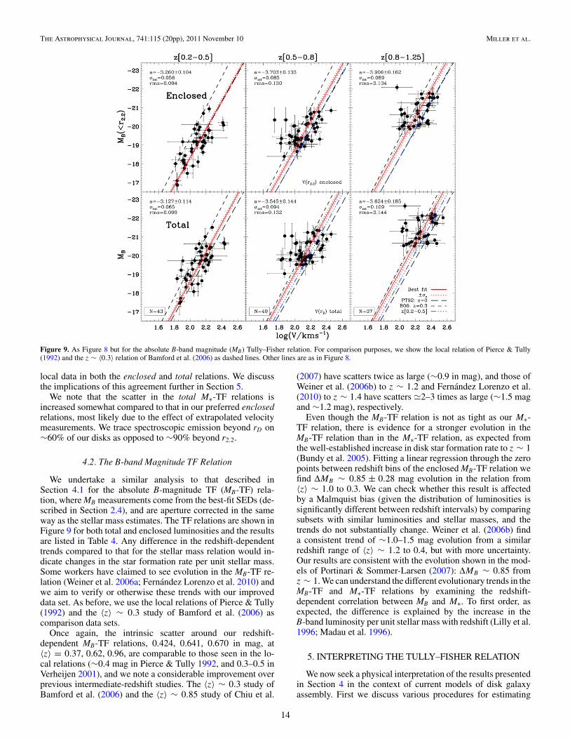
Figure 9. As Figure 8 but for the absolute B-band magnitude (MB) Tully–Fisher relation. For comparison purposes, we show the local relation of Pierce & Tully(1992) and the z ∼ 〈0.3〉 relation of Bamford et al. (2006) as dashed lines. Other lines are as in Figure 8.
local data in both the enclosed and total relations. We discussthe implications of this agreement further in Section 5.
We note that the scatter in the total M∗-TF relations isincreased somewhat compared to that in our preferred enclosedrelations, most likely due to the effect of extrapolated velocitymeasurements. We trace spectroscopic emission beyond rD on∼60% of our disks as opposed to ∼90% beyond r2.2.
4.2. The B-band Magnitude TF Relation
We undertake a similar analysis to that described inSection 4.1 for the absolute B-magnitude TF (MB-TF) rela-tion, where MB measurements come from the best-fit SEDs (de-scribed in Section 2.4), and are aperture corrected in the sameway as the stellar mass estimates. The TF relations are shown inFigure 9 for both total and enclosed luminosities and the resultsare listed in Table 4. Any difference in the redshift-dependenttrends compared to that for the stellar mass relation would in-dicate changes in the star formation rate per unit stellar mass.Some workers have claimed to see evolution in the MB-TF re-lation (Weiner et al. 2006a; Fernandez Lorenzo et al. 2010) andwe aim to verify or otherwise these trends with our improveddata set. As before, we use the local relations of Pierce & Tully(1992) and the 〈z〉 ∼ 0.3 study of Bamford et al. (2006) ascomparison data sets.
Once again, the intrinsic scatter around our redshift-dependent MB-TF relations, 0.424, 0.641, 0.670 in mag, at〈z〉 = 0.37, 0.62, 0.96, are comparable to those seen in the lo-cal relations (∼0.4 mag in Pierce & Tully 1992, and 0.3–0.5 inVerheijen 2001), and we note a considerable improvement overprevious intermediate-redshift studies. The 〈z〉 ∼ 0.3 study ofBamford et al. (2006) and the 〈z〉 ∼ 0.85 study of Chiu et al.
(2007) have scatters twice as large (∼0.9 in mag), and those ofWeiner et al. (2006b) to z ∼ 1.2 and Fernandez Lorenzo et al.(2010) to z ∼ 1.4 have scatters �2–3 times as large (∼1.5 magand ∼1.2 mag), respectively.
Even though the MB-TF relation is not as tight as our M∗-TF relation, there is evidence for a stronger evolution in theMB-TF relation than in the M∗-TF relation, as expected fromthe well-established increase in disk star formation rate to z ∼ 1(Bundy et al. 2005). Fitting a linear regression through the zeropoints between redshift bins of the enclosed MB-TF relation wefind ΔMB ∼ 0.85 ± 0.28 mag evolution in the relation from〈z〉 ∼ 1.0 to 0.3. We can check whether this result is affectedby a Malmquist bias (given the distribution of luminosities issignificantly different between redshift intervals) by comparingsubsets with similar luminosities and stellar masses, and thetrends do not substantially change. Weiner et al. (2006b) finda consistent trend of ∼1.0–1.5 mag evolution from a similarredshift range of 〈z〉 ∼ 1.2 to 0.4, but with more uncertainty.Our results are consistent with the evolution shown in the mod-els of Portinari & Sommer-Larsen (2007): ΔMB ∼ 0.85 fromz ∼ 1. We can understand the different evolutionary trends in theMB-TF and M∗-TF relations by examining the redshift-dependent correlation between MB and M∗. To first order, asexpected, the difference is explained by the increase in theB-band luminosity per unit stellar mass with redshift (Lilly et al.1996; Madau et al. 1996).
5. INTERPRETING THE TULLY–FISHER RELATION
We now seek a physical interpretation of the results presentedin Section 4 in the context of current models of disk galaxyassembly. First we discuss various procedures for estimating
14
The Astrophysical Journal, 741:115 (20pp), 2011 November 10 Miller et al.
Table 4Absolute B-band Magnitude Tully–Fisher Relations
z Range 〈z〉 N aa bb σint,Vc Median σV
d rmsVe σint,M
f Median σMg rmsM
h
Enclosed: MB(r2.2) vs. V(r2.2):
0.2 < z � 1.3 0.64 129 −3.589 −7.546 0.081 0.022 0.127 0.612 0.291 0.9560.2 < z � 0.5 0.37 43 −3.260 ± 0.104 ” fixed 0.056 0.035 0.094 0.425 0.245 0.7110.5 < z � 0.8 0.62 49 −3.703 ± 0.133 ” fixed 0.085 0.045 0.130 0.641 0.364 0.9790.8 < z � 1.3 0.96 37 −3.906 ± 0.162 ” fixed 0.089 0.062 0.134 0.670 0.299 1.011
Total: MB vs. V(rD)
0.2 < z � 1.3 0.64 129 −3.413 −7.754 0.091 0.023 0.130 0.706 0.250 1.0080.2 < z � 0.5 0.37 43 −3.127 ± 0.114 ” fixed 0.065 0.037 0.099 0.505 0.258 0.7710.5 < z � 0.8 0.62 49 −3.545 ± 0.144 ” fixed 0.094 0.057 0.132 0.731 0.364 1.0270.8 < z � 1.3 0.96 37 −3.624 ± 0.185 ” fixed 0.109 0.064 0.144 0.845 0.272 1.114
Notes.a Best-fit y-intercept in mag assuming scatter in V/km s−1 dex.b Slope assuming scatter in V/km s−1 dex.c Internal scatter in V/km s−1 dex.d Median velocity error in V/km s−1 dex.e Total scatter inV/km s−1 dex.f Internal scatter in mag.g Median B-band magnitude error.h Total scatter in mag.
dynamical masses from our rotation curve data (Section 5.1). Wethen derive estimates of the total baryonic mass (Section 5.3).We combine the two estimates to evaluate the relative rolesof baryons and dark matter out to the observable radii probedwith our deep exposures (Section 5.4). Although there areconsiderable uncertainties in what follows, our intent at thisstage is to illustrate the possibilities that will arise when gasmasses can be determined for samples such as ours so that thetotal baryonic components would be accurately measured andtheir role in the TF relation established.
5.1. Dynamical Mass Estimates
The physical basis of our interest in the TF relation is thatthe dynamical mass is strongly correlated with the luminousand stellar mass components of galaxies, and by analyzingempirical constraints, we can gain an understanding of therelative assembly histories of dark and baryonic matter ingalaxies. We thus seek to use our data to estimate both thedynamical masses (i.e., the total mass, including dark andbaryonic) as well as that of the stars and gas. Previous studiesof this nature (Pizagno et al. 2005; Gnedin et al. 2007; Williamset al. 2010, all low-redshift galaxies) derived dynamical massesfrom kinematic data that probe sufficiently far in radius to detectthe dark halo by revealing a deficit of baryons when dynamicmasses are compared to stellar masses.
However, our method of using emission line velocities toestimate the mass within a given radius, such as r2.2, dependssensitively on the assumed shape of the underlying gravitationalpotential, and hence the distribution of mass throughout the disk.For a given ellipsoid potential, the velocity can be most simplyapproximated as
Vc(r)2 ≈ ξGM(r)
r, (6)
where ξ = 1 in the case of spherical symmetry. Assuminga spherical potential will likely overestimate the disk massunless a spherical dark matter halo is dominant within therelevant radius. As such it supplies an effective upper limit
for a given mass of an ellipsoid calculated from the observedcircular velocity. Traditionally, dynamical disk masses havebeen calculated with an exponential “Freeman” potential,solved with modified Bessel functions by assuming a constantmass-to-light ratio and an infinitely thin disk of infinite size(Freeman 1970). This ignores the presence of the bulge andhalo, known to be important even at the scales considered here(e.g., Trott et al. 2010; Dutton et al. 2011b). Therefore, as analternative method of estimating a lower limit, we adopt anoblate potential, characterized by a flattening factor q, which isthe ratio of the scale length normal to the disk over the scalelength of the disk. As shown in Binney & Tremaine (1987), thevelocity for an oblate sphere can then be considered as
Vc(r)2 ≈ 4πGq
∫ r
0
ρ(m2)m2dm√r2 − m2(1 − q2)
, (7)
where m2 = r2 + r2s , and ρ is the assumed density function.
The exact shape of the potential will depend on the relativecontribution of luminous and dark matter, as well as on thetriaxial shape of each component. Although halos are believedto be prolate on large scales, their shape is less clear at thescales considered here. Lensing and dynamical studies of in-dividual systems (Dutton et al. 2011b) suggest that they maybe considerably rounder. Furthermore, the presence of a bulgegenerally implies that the stellar distribution is significantly lessflat than that of a pure disk. We adopt q = 0.4 and an exponen-tial density function as a representative maximum oblateness,equivalent to ξ ≈ 0.752 for Equation (6). If we were to use ade Vaucouleurs profile (Sersic profile where n = 4) instead ofan exponential density profile, ξ would be ≈0.833, resulting ina less than 10% change in the dynamical mass calculation. Inthe following we will consider the q = 1 spherical case andthe q = 0.4 oblate case as bracketing the shape of the total po-tential. Additional systematic uncertainties include the effectsof non-streaming motions, warps and non-gravitational forces,as discussed in the well-established literature on the interpreta-tion of local rotation curves (see Binney & Tremaine 1987 andreferences therein). Finally, we consider possible biases arising
15
The Astrophysical Journal, 741:115 (20pp), 2011 November 10 Miller et al.
from slit spectroscopy and its maximum effect propagated toour dynamical mass estimates in the following section.
5.2. Slit-effect Correction
Recent progress with IFU spectrographs has illustrated somelimitations of traditional long-slit and multi-slit techniquesin determining the internal dynamics of intermediate-redshiftgalaxies. This slit-effect is similar to beam smearing in radioastronomy, where the range of velocities from incoming lightare averaged over the width of the slit, resulting in a broadeningof Doppler shifted lines and an average reduction of therotational velocity. The magnitude of this effect has beenconsidered in detail by Kapferer et al. (2006) and used byFlores et al. (2006) to compare IFU-derived rotational velocitiesto those determined with a multi-slit instrument. Kapfereret al. (2006) systematically investigated the effects of variousslit widths in combination with inclination, spatial binningand position angle offsets on measured disk velocities usingN-body/smoothed particle hydrodynamics simulations. We canuse these results to consider the effect our slit geometry mighthave in distorting our velocities taking into account the galaxysizes and shapes relative to the DEIMOS slits. Kapferer et al.find no systematic bias due to binning and position angle offset(beyond the correction already made, Section 3.2). We can,however, use Kapferer et al.’s results to calculate an upper-limitapproximation of the correction to the velocity V2.2 for the effectof the slit width relative to the scale radius (rs) of each galaxyaccording to its axis ratio (b/a) and for a given inclination i.Derived from Figures 9 and 10 of Kapferer et al. (2006), thecorrection is
Vcorr = Vobs + Vbeam1
(b/a)
rslit
rs
sin i, (8)
where Vbeam ∼ 20 km s−1. We find correlations in the correctionwith respect to scale radius and inclination, but none with mass,redshift, position angle, or observed velocity. The correctionadded to V2.2 ranges from 2 km s−1 to 52 km s−1, with amean of 20 km s−1. These corrections can be found in ourcatalog.
Because of the imprecise nature of these corrections, arisingfrom the fact that the Kapferer et al. result assumes a symmetricGaussian to the spectral line profile (while we fit for two half-Gaussians to account for much of the blending between theseeing and dispersion), the Kapferer et al.-based correctionremains an upper-limit. Thus we did not include them in ourprecisely measured TF relations in Section 4. However, we willapply them to our dynamical mass calculation in order to not biasour estimates in a way that may overestimate the dominance ofthe stellar mass compared to the dark matter. The difference withand without the slit-effect correction can be seen in Figure 10.Because of the imprecision of the analytical formula derivedhere, we strongly advise against applying such a formula beyondits tested range.
5.3. Baryonic Mass Estimates
In order to examine the redshift-dependent fraction of bary-onic mass within r2.2 we need to obtain an estimate of thetotal baryonic mass. In addition to stellar masses, discussed inSection 2.4, we need to account for the presence of gas.
Accurate gas masses are not yet available for intermediate-redshift galaxies, although CO-derived masses have begun toappear for some systems at z > 1 with, e.g., the Plateau de Bure
Interferometer (Tacconi et al. 2010; Daddi et al. 2010). Nonethe-less the situation will improve significantly through upcomingfacilities such as the Atacama Large Millimeter/submillimeterArray, the Meer Karoo Array Telescope, and eventually theSquare Kilometer Array. Although what follows is somewhatspeculative, it provides a reasonable illustration of what willsoon be possible. To make progress, we estimated gas masses(Mg) for our sample using the local stellar-to-gas mass (M∗-to-Mg) ratio as a function of M∗, recently parameterized byPeeples & Shankar (2010) based on H i measures from TheHI Nearby Galaxy Survey (THINGS) and helium-corrected,CO-derived H2 masses from the HERA CO-Line EXtragalac-tic Survey (HERACLES) and the Berkeley–Illinois–MarylandAssociation Survey of Nearby Galaxies (BIMA SONG) (Leroyet al. 2008).
According to the parameterization by Peeples & Shankar(2010):
Mg
M∗= Kf M−γ
∗ (9)
where Kf = 316228, γ = 0.57, and M∗ is measured in units ofsolar masses.
Until precision gas masses become available we cannotbe certain that the Peeples & Shankar (2010) formalism canbe applied in this manner at intermediate redshift. However,locally measured gas-to-stellar mass ratios will underestimatethe gas mass for intermediate-redshift galaxies since many starshave subsequently formed. To correct for this, we consider theobserved evolution in the specific star formation rate (sSFR)for blue galaxies to z ∼ 2 as measured by Oliver et al. (2010).To determine the correction for each galaxy, we integrate thebest-fit sSFR relation out to the relevant redshift. Oliver et al.(2010) find
sSFR = X(1 + z)α, (10)
where log10 X/Gyr−1 = −1.36±0.41 and α = −3.4±0.3. Wetemper this correction by the gas recycling rate (e.g., Kennicuttet al. 1994; Madau et al. 1998; Cole et al. 2001), estimated tobe ∼40% for a Chabrier (2003) IMF from z ∼ 1 to present.This scenario is not strictly a closed-box model, where a galaxysits in a huge reservoir of gas and simply converts that gas tostars over time. For one, we include the substantial Chabrierrecycling rate consistent with the IMF we assume in our stellarmass estimates. The scenario we present here is also consistentwith roughly equal inflow and outflow since z ∼ 1. The fractionof feedback-driven material that exceeds the escape velocityof the galaxy’s potential well, and also the typical redshifts atwhich the filaments that feed galaxies evaporate, are still largelyunknown. The gas mass estimates we add to our stellar massesare on average 30% of the total stellar mass estimates, and onlyexceed that of the stellar mass in a few of the lowest massobjects. So we claim that our gas mass estimates are not themain drivers of our conclusions, and each galaxy’s stellar massand redshift essentially determine the gas mass estimate for thisscenario.
5.4. Comparison of Baryonic and Dynamical Masses
We finally turn to our comparison of the dynamical mass withthe stellar and baryonic mass. The results of this comparisonare given in Figure 10. The top panels show the stellar-to-dynamical mass ratio for a spherical and oblate potential.Across our redshift range we find our stellar-to-dynamicalmass fractions are ∼0.3 for a spherical potential and ∼0.4 foran oblate potential, with considerable scatter. The dynamical
16
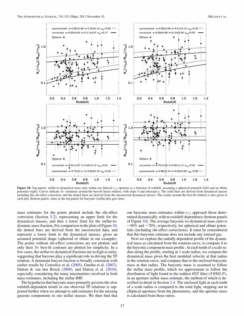
The Astrophysical Journal, 741:115 (20pp), 2011 November 10 Miller et al.
Figure 10. Top panels: stellar-to-dynamical mass ratio within our fiducial r2.2 aperture as a function of redshift, assuming a spherical potential (left) and an oblatepotential (right). Curves indicate 3σ variations around the best-fit linear relation, with slope b and intercept a. The solid lines are derived from dynamical massesincluding the slit-effect correction, and the dotted lines are derived from the uncorrected dynamical masses. The scatter around the best-fit relation is also given ineach plot. Bottom panels: same as the top panels for baryonic (stellar plus gas) mass.
mass estimates for the points plotted include the slit-effectcorrection (Section 5.2), representing an upper limit for thedynamical masses, and thus a lower limit for the stellar-to-dynamic mass fraction. For comparison in the plots of Figure 10,the dotted lines are derived from the uncorrected data, andrepresent a lower limit to the dynamical masses, given anassumed potential shape (spheroid or oblate in our example).The points without slit-effect corrections are not plotted, andonly their 3σ best-fit contours are plotted for simplicity. In afew cases, the stellar-to-dynamical fractions are as high as unity,suggesting that baryons play a significant role in driving the TFrelation. A dominant baryon fraction is broadly consistent withearlier results by Conselice et al. (2005), Gnedin et al. (2007),Dutton & van den Bosch (2009), and Dutton et al. (2010),especially considering the many uncertainties involved in bothmass estimates, including the stellar IMF.
The hypothesis that baryonic mass primarily governs the slowredshift-dependent trends in our observed TF relations is sup-ported further when we attempt to add estimates for the missinggaseous components to our stellar masses. We then find that
our baryonic mass estimates within r2.2 approach those deter-mined dynamically, with no redshift dependence (bottom panelsof Figure 10). The average baryonic-to-dynamical mass ratio is∼50% and ∼70%, respectively, for spherical and oblate poten-tials (including slit-effect corrections). It must be rememberedthat this baryonic estimate does not include any ionized gas.
Next we explore the radially dependent profile of the dynam-ical mass as calculated from the rotation curve, to compare it tothe baryonic component mass profile. At each tenth of a scale ra-dius along the profile, starting at 1 scale radius, we compute thedynamical mass given the best modeled velocity at that radiusin the rotation curve, and compare that to the enclosed baryonicmass at that radius. The baryonic mass is assumed to followthe stellar mass profile, which we approximate to follow thedistribution of light found in the reddest HST filter (F850LP ),in an aperture stellar mass estimate, the method of which is de-scribed in detail in Section 2.4. The enclosed light at each tenthof a scale radius is compared to the total light, stepping out inelliptical apertures from the photometry, and the aperture massis calculated from these ratios.
17
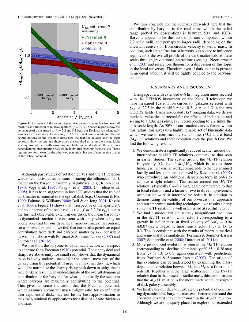
The Astrophysical Journal, 741:115 (20pp), 2011 November 10 Miller et al.
Figure 11. Estimates of the mean baryonic-to-dynamical mass fraction over allredshifts as a function of relative aperture (f = r/rs ). Shaded regions show thepercentage of disks traced to f = 2.2 and 3.2 (rD); our Keck survey adequatelysamples the rotational velocities to f �3.5. Different curves relate to differentdeterminations of the dynamic mass (see the text for details) and the tightcontours show the one and three times the standard error on the mean. Lightshading around the results assuming an oblate potential indicate the aperture-dependent region containing 68% of the individual fractions for our disks. Theseregions are not shown for the other two potentials, but are of similar size to thatof the oblate potential.
Although past studies of rotation curves and the TF relationwere often motivated as a means of tracing the influence of darkmatter on the baryonic assembly of galaxies, (e.g., Rubin et al.1980; Vogt et al. 1997; Pizagno et al. 2005; Conselice et al.2005), it has been suggested in local TF studies that the role ofdark matter is minimal in the optical disk (e.g., Courteau & Rix1999; Palunas & Williams 2000; Bell & de Jong 2001; Kassinet al. 2006). Figure 11 shows that, irrespective of the aperture f,defined in terms of the scale radius (i.e., f = 2.2 for r2.2), out tothe furthest observable extent in our disks, the mean baryonic-to-dynamical fraction is consistent with unity when using anoblate potential for our dynamical mass estimates. In contrast,for a spherical potential, we find that our results permit an equalcontribution from dark and baryonic matter by r2.2, consistentas we noted above with Portinari & Sommer-Larsen (2007) andDutton et al. (2011c).
We also show the baryonic-to-dynamical fraction with respectto aperture for a Freeman (1970) potential. The unphysical andsharp rise above unity for small radii shows that the dynamicalmass is likely underestimated for the central-most part of thegalaxy using this potential. If used in a maximal disk fit, whichwould re-normalize the sharply rising peak down to unity, the fitwould likely result in an underestimate of the overall dynamicalcontribution of the baryons for what is nominally the scenariowhere baryons are maximally contributing to the potential.This gives us some indication that the Freeman potential,which assumes a constant mass-to-light ratio for an infinitelythin exponential disk, may not be the best approximation inmaximal/minimal fit applications for a disk of a finite thicknessand size.
We thus conclude for the scenario presented here that thecontribution by baryons to the total mass within the radialrange probed by observations is between 50% and 100%.Baryons appear to be the most important component within2.2 scale radii, and perhaps to larger radii, depending on theuncertain conversion from circular velocity to stellar mass. Inaddition, such a high fraction of baryons is expected to influencesignificantly the overall profile of the dark matter halo at thesescales through gravitational interactions (see, e.g., Noordermeeret al. 2007 and references therein for a discussion of this topicin the local universe). Therefore even if dark matter is presentin an equal amount, it will be tightly coupled to the baryoniccontent.
6. SUMMARY AND DISCUSSION
Using spectra with extended 6–8 hr integration times securedwith the DEIMOS instrument on the Keck II telescope wehave measured 129 rotation curves for galaxies selected withzAB < 22.5 in the redshift range 0.2 < z < 1.3 in the twoGOODS fields. Using associated HST imaging data, we derivemodeled velocities corrected for the effects of inclination andseeing to a fiducial radius, r2.2, corresponding to 2.2 times thedisk scale length. As 90% of our rotation curves flatten withinthis radius, this gives us a highly reliable set of kinematic datawhich we use to construct the stellar mass (M∗) and B-band(MB) TF relations and their evolution over the past 8 Gyr. Wefind the following results.
1. We demonstrate a significantly reduced scatter around ourintermediate-redshift TF relations compared to that seenin earlier studies. The scatter around the M∗-TF relationis typically 0.2 dex of M∗/M�, which is two to threetimes less than earlier work, comparable to that determinedlocally and less than that achieved by Kassin et al. (2007)who introduced an additional dispersion term in order toachieve a tight relation. The scatter around our MB-TFrelation is typically 0.4–0.7 mag, again comparable to thatin local relations and a factor of two to three improvementover earlier work at intermediate redshift. In addition todemonstrating the validity of our observational approachand our improved modeling techniques, our results clearlyshow the TF relation is well established at redshift z � 1.
2. We find a modest but statistically insignificant evolutionin the M∗-TF relation with redshift corresponding to agrowth in stellar mass at fixed velocity of ΔM∗ = 0.04±0.07 dex with cosmic time from a redshift 〈z〉 � 1.0 to0.3. This is consistent with the results of recent numericaland semi-analytic simulations (Portinari & Sommer-Larsen2007; Somerville et al. 2008; Dutton et al. 2011a).
3. More pronounced evolution is seen in the MB-TF relationcorresponding to a decline in luminosity of 0.85 ± 0.28 magfrom 〈z〉 � 1.0 to 0.3, again consistent with predictionsfrom Portinari & Sommer-Larsen (2007). The origin ofthis evolution can be understood by examining the mass-dependent correlation between M∗ and MB as a function ofredshift. Together with the larger scatter seen in the MB-TFrelation than in that based on stellar mass, this demonstratesthat the M∗-TF relation is the more fundamental descriptorof disk galaxy assembly.
4. We finally use our data to illustrate the potential of compar-ing dynamical and baryonic masses to better understand thecontributions that they matter make in the M∗-TF relation.Although we are uniquely placed to explore our extended
18
The Astrophysical Journal, 741:115 (20pp), 2011 November 10 Miller et al.
rotation curves and carefully derived stellar masses, ourgas mass estimates are clearly approximate at this stage.We estimate dynamical masses using both spherical andoblate potentials which we expect bracket the likely values.We compute baryonic masses by estimating the additionalmass in cold gas. We find that baryons may contribute be-tween 50% and 100% of the total mass within the radiiat which we can confidently observe dynamics of the gasin our disk sample. Such a high fraction of baryons influ-ence significantly the overall profile of the dark matter halo.Even if dark matter is present in an equal amount, it will betightly coupled to the baryonic content.
S.H.M. thanks the Rhodes Trust, the Oxford AstrophysicsDepartment, New College, Oxford, and the California Insti-tute of Technology for supporting her work. M.S. and R.S.E.acknowledge financial support from the Royal Society. Wethank S. Moran, N. Miller, G. Mikelsons, and K. Chiu forconsiderable initial assistance with the organization of thisdata set. We thank C. Peng for supplying us with galfit3.0 and acknowledge useful discussions with A. Benson,A. Brooks, A. Bunker, M. Bureau, M. Cappellari, R. Davies,H. Flores, F. Hammer, S. Kassin, L. Miller, and M. Puech.The referee, B. Weiner, is acknowledged for his constructivecomments in the improvement of this paper. The spectroscopicdata was secured with the W. M. Keck Observatory on MaunaKea. We thank the observatory staff for their dedication andsupport. The authors recognize and acknowledge the culturalrole and reverence that the summit of Mauna Kea has alwayshad with the indigenous Hawaiian community. We are most for-tunate to have the opportunity to conduct observations from thismountain.
REFERENCES
Atkinson, N., Conselice, C. J., & Fox, N. 2007, arXiv:0712.1316Bamford, S. P., Aragon-Salamanca, A., & Milvang-Jensen, B. 2006, MNRAS,
366, 308Bell, E. F., & de Jong, R. S. 2001, ApJ, 550, 212Benson, A. J., Bower, R. G., Frenk, C. S., et al. 2003, ApJ, 599, 38Binney, J., & Tremaine, S. 1987, Galactic Dynamics (Princeton, NJ: Princeton
Univ. Press)Blumenthal, G. R., Faber, S. M., Flores, R., & Primack, J. R. 1986, ApJ, 301,
27Bohm, A., & Ziegler, B. L. 2007, in ASP Conf. Ser. 379, Cosmic Frontiers, ed.
N. Metcalfe & T. Shanks (San Francisco, CA: ASP), 278Bohm, A., Ziegler, B. L., Saglia, R. P., et al. 2004, A&A, 420, 97Brinchmann, J., & Ellis, R. S. 2000, ApJ, 536, L77Bruzual, G., & Charlot, S. 2003, MNRAS, 344, 1000Bundy, K., Ellis, R. S., & Conselice, C. J. 2005, ApJ, 625, 621Bundy, K., Fukugita, M., Ellis, R. S., et al. 2009, ApJ, 697, 1369Chabrier, G. 2003, PASP, 115, 763Chiu, K., Bamford, S. P., & Bunker, A. 2007, MNRAS, 377, 806Coil, A. L., Davis, M., Madgwick, D. S., et al. 2004, ApJ, 609, 525Cole, S., Norberg, P., Baugh, C. M., et al. 2001, MNRAS, 326, 255Conselice, C. J., Bundy, K., Ellis, R. S., et al. 2005, ApJ, 628, 160Courteau, S. 1996, ApJS, 103, 363Courteau, S. 1997, AJ, 114, 2402Courteau, S., & Rix, H. 1997, BAAS, 29, 1332Courteau, S., & Rix, H.-W. 1999, ApJ, 513, 561Cresci, G., Hicks, E. K. S., Genzel, R., et al. 2009, ApJ, 697, 115Daddi, E., Bournaud, F., Walter, F., et al. 2010, ApJ, 713, 686Dalcanton, J. J., Spergel, D. N., & Summers, F. J. 1997, ApJ, 482, 659Davis, M., Faber, S. M., Newman, J., et al. 2003, Proc. SPIE, 4834, 161Dickinson, M., Giavalisco, M., & GOODS Team. 2003, in The Mass of
Galaxies at Low and High Redshift, ed. R. Bender & A. Renzini (Berlin:Springer), 324
Dutton, A. A., Bosch, F. C. V. D., Faber, S. M., et al. 2011a, MNRAS, 410, 1660Dutton, A. A., Brewer, B. J., Marshall, P. J., et al. 2011b, arXiv:1101.1622
Dutton, A. A., Conroy, C., van den Bosch, F. C., Prada, F., & More, S.2010, MNRAS, 407, 2
Dutton, A. A., Conroy, C., van den Bosch, F. C., et al. 2011c, MNRAS, 416,322
Dutton, A. A., & van den Bosch, F. C. 2009, MNRAS, 396, 141Dutton, A. A., van den Bosch, F. C., Dekel, A., & Courteau, S. 2007, ApJ, 654,
27Eke, V. R., Navarro, J. F., & Steinmetz, M. 2001, ApJ, 554, 114Ellis, R., & Silk, J. 2009, New Frontiers in Cosmology and Galaxy Formation:
Challenges for the Future (Cambridge: Cambridge Univ. Press), 133Faber, S. M., Phillips, A. C., Kibrick, R. I., et al. 2003, Proc. SPIE, 4841, 1657Faber, S. M., Willmer, C. N. A., Wolf, C., et al. 2007, ApJ, 665, 265Fall, S. M., & Efstathiou, G. 1980, MNRAS, 193, 189Fernandez Lorenzo, M., Cepa, J., Bongiovanni, A., et al. 2009, A&A, 496, 389Fernandez Lorenzo, M., Cepa, J., Bongiovanni, A., et al. 2010, A&A, 521, A27Flores, H., Hammer, F., Puech, M., Amram, P., & Balkowski, C. 2006, A&A,
455, 107Forster Schreiber, N. M., Genzel, R., Bouche, N., et al. 2009, ApJ, 706, 1364Freeman, K. C. 1970, ApJ, 160, 811Genzel, R., Tacconi, L. J., Eisenhauer, F., et al. 2006, Nature, 442, 786Giavalisco, M., Ferguson, H. C., Koekemoer, A. M., et al. 2004, ApJ, 600, L93Gnedin, O. Y., Weinberg, D. H., Pizagno, J., Prada, F., & Rix, H. 2007, ApJ,
671, 1115Gnerucci, A., Marconi, A., Cresci, G., et al. 2011, A&A, 528, 88Governato, F., Willman, B., Mayer, L., et al. 2007, MNRAS, 374, 1479Haynes, M. P., & Giovanelli, R. 1984, AJ, 89, 758Jones, T., Ellis, R., Jullo, E., & Richard, J. 2010, ApJ, 725, L176Kapferer, W., Ferrari, C., Domainko, W., et al. 2006, A&A, 447, 827Kassin, S. A., de Jong, R. S., & Weiner, B. J. 2006, ApJ, 643, 804Kassin, S. A., Weiner, B. J., Faber, S. M., Koo, D. C., & Lotz, J. M. 2007, in
ASP Conf. Ser. 380, Deepest Astronomical Surveys, ed. J. Afonso, H. C.Ferguson, B. Mobasher, & R. Norris (San Francisco, CA: ASP), 477
Kelly, B. C. 2007, ApJ, 665, 1489Kennicutt, R. C., Jr., Tamblyn, P., & Congdon, C. E. 1994, ApJ, 435, 22Le Fevre, O., Vettolani, G., Paltani, S., et al. 2004, A&A, 428, 1043Leroy, A. K., Walter, F., Brinks, E., et al. 2008, AJ, 136, 2782Lilly, S. J., Le Fevre, O., Hammer, F., & Crampton, D. 1996, ApJ, 460, L1Madau, P., Ferguson, H. C., Dickinson, M. E., et al. 1996, MNRAS, 283, 1388Madau, P., Pozzetti, L., & Dickinson, M. 1998, ApJ, 498, 106Markwardt, C. B. 2009, in ASP Conf. Ser. 411, ed. D. A. Bohlender, D. Durand,
& P. Dowler (San Francisco, CA: ASP), 251Meyer, M. J., Zwaan, M. A., Webster, R. L., Schneider, S., & Staveley-Smith,
L. 2008, MNRAS, 391, 1712Mo, H. J., & Mao, S. 2000, MNRAS, 318, 163Mo, H. J., Mao, S., & White, S. D. M. 1998, MNRAS, 295, 319Moran, S. M., Miller, N., Treu, T., Ellis, R. S., & Smith, G. P. 2007, ApJ, 659,
1138Noordermeer, E., van der Hulst, J. M., Sancisi, R., Swaters, R. S., & van Albada,
T. S. 2007, MNRAS, 376, 1513Oliver, S., Frost, M., Farrah, D., et al. 2010, MNRAS, 405, 2279Palunas, P., & Williams, T. B. 2000, AJ, 120, 2884Peeples, M. S., & Shankar, F. 2010, arXiv:1007.3743Peng, C. 2010, BAAS, 42, 578Persic, M., Salucci, P., & Stel, F. 1996, MNRAS, 281, 27Pierce, M. J., & Tully, R. B. 1992, ApJ, 387, 47Piontek, F., & Steinmetz, M. 2011, MNRAS, 410, 2625Pizagno, J., Prada, F., Weinberg, D. H., et al. 2005, ApJ, 633, 844Portinari, L., & Sommer-Larsen, J. 2007, MNRAS, 375, 913Puech, M., Flores, H., Hammer, F., et al. 2008, A&A, 484, 173Retzlaff, J., Rosati, P., Dickinson, M., et al. 2010, A&A, 511, A50Rix, H., Guhathakurta, P., Colless, M., & Ing, K. 1997, MNRAS, 285, 779Rubin, V. C., Ford, W. K. J., & Thonnard, N. 1980, ApJ, 238, 471Seljak, U., Makarov, A., McDonald, P., et al. 2005, Phys. Rev. D, 71, 103515Shapiro, K. L., Genzel, R., Forster Schreiber, N. M., et al. 2008, ApJ, 682, 231Shlosman, I. 2009, in ASP Conf. Ser. 419, ed. S. Jogee, I. Marinova, L. Hao, &
G. A. Blanc (San Francisco, CA: ASP), 39Somerville, R. S., Barden, M., Rix, H., et al. 2008, ApJ, 672, 776Spergel, D. N., Bean, R., Dore, O., et al. 2007, ApJS, 170, 377Stark, D. P., Swinbank, A. M., Ellis, R. S., et al. 2008, Nature, 455, 775Steinmetz, M., & Navarro, J. F. 1999, ApJ, 513, 555Tacconi, L. J., Genzel, R., Neri, R., et al. 2010, Nature, 463, 781Trott, C. M., Treu, T., Koopmans, L. V. E., & Webster, R. L. 2010, MNRAS,
401, 1540Tully, R. B., & Fisher, J. R. 1977, A&A, 54, 661Tully, R. B., Pierce, M. J., Huang, J., et al. 1998, AJ, 115, 2264van den Bosch, F. C. 2000, ApJ, 530, 177Verheijen, M. A. W. 2001, ApJ, 563, 694
19
The Astrophysical Journal, 741:115 (20pp), 2011 November 10 Miller et al.
Vogt, N. P., Forbes, D. A., Phillips, A. C., et al. 1996, ApJ, 465, L15Vogt, N. P., Phillips, A. C., Faber, S. M., et al. 1997, ApJ, 479, L121Wechsler, R. H., Bullock, J. S., Primack, J. R., Kravtsov, A. V., & Dekel, A.
2002, ApJ, 568, 52Weiner, B. J., Willmer, C. N. A., Faber, S. M., et al. 2006a, ApJ, 653, 1049Weiner, B. J., Willmer, C. N. A., Faber, S. M., et al. 2006b, ApJ, 653, 1027
Williams, M. J., Bureau, M., & Cappellari, M. 2010, MNRAS, 409, 1330Willick, J. A. 1999, ApJ, 516, 47Wirth, G. D., Willmer, C. N. A., Amico, P., et al. 2004, AJ, 127, 3121Wolf, C., Meisenheimer, K., Kleinheinrich, M., et al. 2004, A&A, 421,
913Ziegler, B. L., Bohm, A., Fricke, K. J., et al. 2002, ApJ, 564, L69
20

![Secular Evolution in Disk Galaxies ToappearinRMParXiv:1310.0403v2 [astro-ph.GA] 11 Dec 2013 Secular Evolution in Disk Galaxies ToappearinRMP JASellwood Department of Physics & Astronomy,](https://img.pdfslide.us/doc/110x75/5fe83c34b2f00f3a82491691/secular-evolution-in-disk-galaxies-toappearinrmp-arxiv13100403v2-astro-phga.jpg)