The Art of Modeling Financial Options: Monte Carlo

Simulation

Antonie Kotzea, Rudolf Oosthuizenb

aSenior Research Associate, Faculty of Economic and Financial SciencesDepartment of Finance and Investment Management, University of Johannesburg

PO Box 524, Aucklandpark 2006, South AfricabThe JSE, One Exchange Square, Gwen Lane, Sandown, 2196, South Africa

Tel: +2711-520-7000

Abstract

Modeling is important because scientists investigate the world around us by building modelsthat simulate real-world problems. Modeling is neither science nor mathematics; it is thecraft that builds bridges between the two. Progress in modeling dynamics has alwaysbeen closely associated with advances in computing. Monte Carlo simulation/modeling orprobability simulation is a technique frequently used in the financial markets to understandcomplex financial instruments. It is used to scrutinise the impact of risk and uncertainty infinancial and other forecasting models. It is very useful when complex financial instrumentsneed to be priced. Exotic options are listed on the JSE on its Can-Do platform. Mostlisted exotic options are marked-to-model and the JSE needs accurate values at the endof every day. Monte Carlo methods in a local volatility framework are implemented. Thispaper discusses how Monte Carlo (MC) simulation is implemented when exotic options likeBarriers are valued. We further summarise the historical development in modern computingand the development of the Monte Carlo method.

Keywords: Exotic options, JSE, Can-Do Options, Implied Volatility, Local Volatility,Dupire Transforms, Gyongy Theorem, Barrier options, Monte Carlo simulation,Feynmann-Kac Theorem

(JEL) Classification: C15, C61, C63, G13, G17

Email addresses: antonie@quantonline.co.za; http://www.quantonline.co.za (AntonieKotze), croosthuizen@gmail.com (Rudolf Oosthuizen)

1

1. Introduction

Why is simulation or modeling an important component of analysis for scientists?Simulation is the imitation of a real-world process or system. The “joy of simulation”is that one does not need to own or rent a Boeing 777 or Airbus A380 to fly them!Simulation games are fun too and one gains valuable experience at the same time.Experience and insight are gained by simulating the valuation of financial products,constructing portfolios and testing trading rules (McLeish, 2005). Through simulationwork is transferred to a computer. Models can be handled that involve greater com-plexity and fewer assumptions, and a more faithful representation of the real worldis possible. Morrison (2008) states that modeling is neither science nor mathematics;it is the craft that builds bridges between the two.

Modeling is important because scientists investigate the world around us by build-ing models that simulate real-world problems. Our insight in a physical system, com-bined with numerical mathematics, gives us the rules for setting up an algorithm (themodel), or a set of rules for solving a particular problem (Steinhauser, 2013). Thesemodels usually take the form of differential equations that have to be solved to obtainphysical answers. Researchers usually start with a very simplistic model and try tosolve it analytically or algebraically. Such models are mostly easier to analyse andscrutinise. This inevitably means they have to make a lot of simplifying assumptions.As they start to understand the dynamics of this “toy” model, they add more com-plexity to make it more representative of the real world problem under investigation— after theory encounters fact, the modelers revise their equations and computerprograms. This means that modeling practitioners need to be familiar with a widevariety of mathematical specialities, computer science and one or more disciplineswhich provide data.

This is exactly the route the evolution of the Black-Scholes option pricing modeltook. Black, Scholes and Merton made some simplifying assumptions that enabledthem to devise a backward parabolic partial differential equation (PDE). Black &Scholes (1973) used a bond and hedge replication strategy to derive their PDE whileMerton (1973) made this argument more rigorous and general. They solved this PDEanalytically using Fourier series methods.

It is now well-known that this model is far from the real world and stock pricesbehave in a much more complex manner. Black (1988) discussed the deficiencies andKotze (2003) emphasised the consequences of this simple model. Since 1973 most ofthe original simplifying assumptions have been relaxed. When some of these assump-tions are relaxed, one finds that the model cannot be solved analytically anymore.This is, however, not discouraging because simulation and modeling techniques areusually great “complex problem solvers.”

Monte Carlo simulation has become an essential tool in the pricing of derivativesecurities and the management of risk. Most problems where there is significantuncertainty, can be solved using Monte Carlo techniques. Monte Carlo methodsare techniques utilising random numbers and probability to solve problems. Theanalysis is based on artificially recreating a chance process, running it many timesand directly observing the results. Glassermann (2004) states it is thus based on the

2

analogy between probability and volume.Monte Carlo methods are attractive in evaluating integrals in high dimensions

(Glassermann, 2004). What does this have to do with financial engineering? Thefoundation of the theory of derivative pricing is the random walk of asset prices. Thisis known as the Black-Scholes theory and leads to the Black-Scholes parabolic partialdifferential equation (PDE). According to the Feynman-Kac theorem, the solution tothis PDE can be represented by an expected value — valuing derivatives is reducedto computing expectations. Monte Carlo simulation is widely used in statistics incalculating an expected value of a particular function. Boyle (1977) showed that allfinancial options are always the expected value of certain functions. If we were towrite the relevant expectation as an integral, we would find that its dimension islarge or infinite. This is precisely the setting in which Monte Carlo methods becomeattractive (Glassermann, 2004).

Weber (2011) stated that the Monte Carlo method is widely used in the financialmarkets as a valuation tool. It is used with path-dependent options and in modelswith more than one state variable. It is sometimes preferred to finite difference or treemethods, even in situations where these methods could work well — simply becauseits generality and its robustness in contexts where a portfolio of options is beingvalued.

In this paper, we consider the Monte Carlo approach to value exotic options. TheJSE has listed exotic options and structured products on their Can-Do platform1.Kotze & Oosthuizen (2013) discussed and explained the local volatility pricing ofexotic Can-Do options like Barrier options, as well as the methodologies used to de-termine their initial margins. Local volatility models have been in use since the 1980salthough these were not known by the name “local volatility.” The mathematicalframework for local volatility was first formulated by Dupire (1994). At the sametime, Derman & Kani (1994) and Rubinstein (1994) solved this problem numericallyby implementing binomial trees. These methods have subsequently been improvedby many other researchers (Andersen & Andreasen, 2000; Lagnado & Osher, 1997).It has since been realised that Dupire’s framework is an extension of research doneby Gyongy (1986).

Many exotic options, like Barrier options, have Black-Scholes type closed formvaluation formulas (Rubinstein & Reiner, 1991; Haug, 2007; Bouzoubaa & Osserein,2010). However, it is also known that these formulas do not lead to market related andrealistic prices and hedge ratios. This is due to the assumption of a fixed volatility.However, such option are path-dependent meaning that the actual path the stocktakes to get to the expiry value on the expiry date does matter. To price themcorrectly one should either use stochastic volatility models or local volatility models.The choice here is to use either finite difference techniques or Monte Carlo simulation.This note will focus on Monte Carlo techniques.

The layout of this paper is as follows: In section 2 we give some history on the

1http://www.jse.co.za/Products/Equity-Derivatives-Market/

Equity-Derivatives-Product-Detail/Can-Do_Futures_and_Options.aspx

3

origins of computing and Monte Carlo simulation. Section 3 gives a brief overview ofexotic options. In section 4 we bring local volatility into the Black-Scholes frameworkand we discretise the Black-Scholes stochastic differential equation. Section 5 is crucialwhere we show how to use Monte Carlo simulation when pricing options. Section 6discusses Dupire’s local volatility mapping and in section 7 we use Dupire to price asingle barrier option. We conclude in section 8.

Note that there are three Appendices where we elaborate on some of the theorydescribed in this paper. Appendix A shows why Monte Carlo simulation can beused when pricing options and we show how to discretise the Black-Scholes stochasticdifferential equation. In Appendix B we discuss the generation of random numbersand in Appendix C we elaborate on convergence issues when simulating stock pricepaths and option values.

2. A Lesson in History

Progress in modeling dynamics2 has always been associated with advances incomputing (Morrison, 2008). As such dynamics has reached maturity with the devel-opment of digital computers, both as concept and technological product.

But, why is reading the history of science important? Donald Knuth motivates,why, as a computer scientist he reads the history of science. First, reading historyhelped him to understand the process of discovery. Second, understanding the diffi-culty and false starts experienced by brilliant historical scientists in making discoveriesthat specialists now find obvious helped him to see what made concepts challengingto students and thus to become a “much better writer and teacher.” Third, appreci-ating the historical contribution of non-Western scientists helped in “celebrating thecontributions of many cultures.” Fourth, history is the craft of telling stories, whichis “the best way to teach, to explain something.” Fifth, the biographies of scientiststeach tactics for a successful and rewarding career. Sixth, history teaches how humanexperience has changed over time. As humans we should care about that (Haigh,2015).

2.1. A bit of Computing History

The modern history of computing is quite short (Copeland, 2008). In 1623. Wil-helm Schickard (1592-1635), constructed a machine for his mathematician friend Jo-hannes Kepler (1571-1630) which was able to perform addition, subtraction, multi-plication and division (Steinhauser, 2013).

Charles Babbage (1792-1871) is generally credited with originating the concept ofa programmable computer (Dasgupta, 2014). Babbage built a small working modelin 1822 but he never completed a full-scale machine. We had to wait until 1990 whenthe Science Museum3 in London built Babbage’s Difference Engine No. 2 from hisoriginal designs (Swade, 2005). The punch card was developed by Hermann Hollerith(1860-1929) during 1890. It was developed for a population census.

2Dynamic means changing. Dynamical is what concerns change.3http://www.sciencemuseum.org.uk/onlinestuff/stories/babbage.aspx

4

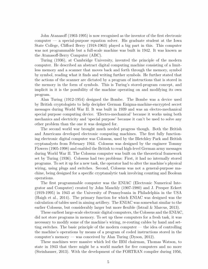
John Atanasoff (1903-1995) is now recognised as the inventor of the first electroniccomputer — a special-purpose equation solver. His graduate student at the IowaState College, Clifford Berry (1918-1963) played a big part in this. This computerwas not programmable but a full-scale machine was built in 1942. It was known asthe Atanasoff-Berry Computer (ABC).

Turing (1936), at Cambridge University, invented the principle of the moderncomputer. He described an abstract digital computing machine consisting of a limit-less memory and a scanner that moves back and forth through the memory, symbolby symbol, reading what it finds and writing further symbols. He further stated thatthe actions of the scanner are dictated by a program of instructions that is stored inthe memory in the form of symbols. This is Turing’s stored-program concept, andimplicit in it is the possibility of the machine operating on and modifying its ownprogram.

Alan Turing (1912-1954) designed the Bombe. The Bombe was a device usedby British cryptologists to help decipher German Enigma-machine-encrypted secretmessages during World War II. It was built in 1939 and was an electro-mechanicalspecial purpose computing device. ‘Electro-mechanical’ because it works using bothmechanics and electricity and ‘special purpose’ because it can’t be used to solve anyother problem than the one it was designed for.

The second world war brought much needed progress though. Both the Britishand Americans developed electronic computing machines. The first fully function-ing electronic digital computer was Colossus, used by the Bletchley Park and Britishcryptanalysts from February 1944. Colossus was designed by the engineer TommyFlowers (1905-1998) and enabled the British to read high-level German army messagesduring World War II. The Colossus computer was built on the theoretical frameworkset by Turing (1936). Colossus had two problems: First, it had no internally storedprograms. To set it up for a new task, the operator had to alter the machine’s physicalwiring, using plugs and switches. Second, Colossus was not a general-purpose ma-chine, being designed for a specific cryptanalytic task involving counting and Booleanoperations.

The first programmable computer was the ENIAC (Electronic Numerical Inte-grator and Computer) created by John Mauchly (1907-1980) and J. Presper Eckert(1919-1995) in 1943 at the University of Pennsylvania in Philadelphia in the USA(Haigh et al., 2014). The primary function for which ENIAC was designed was thecalculation of tables used in aiming artillery. The ENIAC was somewhat similar to theearlier Colossus, but considerably larger but more flexible (Istrail & Marcus, 2013).

These earliest large-scale electronic digital computers, the Colossus and the ENIAC,did not store programs in memory. To set up these computers for a fresh task, it wasnecessary to modify some of the machine’s wiring, re-routing cables by hand and set-ting switches. The basic principle of the modern computer — the idea of controllingthe machine’s operations by means of a program of coded instructions stored in thecomputer’s memory — was conceived by Alan Turing (Dyson, 2012).

These machines were massive which led the IBM chairman, Thomas Watson, tostate in 1943 that there might be a world market for five computers and no more(Steinhauser, 2013). With the development of the FORTRAN compiler during 1956,

5

modeling and simulation became a lot easier and accessible.

2.2. The History of Monte Carlo Simulation

The ‘Monte Carlo’ method was developed by the physicists and mathematiciansworking on the Manhattan Project4 during the second world war. The main characterwas Stanilaw Ulam (1909-1984). Ulam and Edward Teller (1908-2003) developed thefirst thermonuclear weapon also known as the hydrogen bomb or H-bomb. Ulam wasintensely interested in random processes. He relaxed by playing solitaire and poker.The name ‘Monte Carlo’ was coined by Nicholas Metropolis (1915-1999) during 1947because Ulam had often mentioned his uncle, Michal Ulam, “who just had to go toMonte Carlo” to gamble.

It all started in October 1943 when Ulam received an invitation to join the Man-hattan Project at the secret Los Alamos Laboratory in New Mexico. His extensivemathematical background made him aware that statistical sampling techniques hadfallen into desuetude because of the length and tediousness of the calculations. It isbelieved that the first real application of the ‘statistical sampling method’ was un-dertaken by Enrico Fermi (1901-1954) in the 1930s. Due to the computational issues,this method did not really take off.

But, Los Alamos had access to the ENIAC. Access to this toy convinced Ulam thatFermi’s statistical techniques should be resuscitated, and he discussed this idea withJohn von Neumann (1903-1957) — a principle member of the Manhattan Project5.This triggered the spark that led to the Monte Carlo method. One of the first problemssolved on the ENIAC in 1946 was a computational model of a thermonuclear reaction6.Metropolis & Ulam (1949) published the first unclassified paper on the Monte Carlomethod in 1949.

Los Alamos got its own computer early in 1952. It was called the MANIAC (Math-ematical Analyzer, Numerical Integrator, and Computer or Mathematical Analyzer,Numerator, Integrator, and Computer). Enrico Fermi joined Los Alamos during thesummer of 1952 and used the MANIAC to solve many statistical problems. A signif-icant advance in the use of the Monte Carlo method came out of the collaborationbetween Nicholas Metropolis and Edward Teller. Together they introduced the ideaof what is today known as importance sampling, also referred to as the Metropolisalgorithm7.

2.3. Monte Carlo Methods and the Pricing of Options

Boyle (1977) was the first to relate the pricing of options to the simulation ofrandom asset paths. He showed how to find the fair value of an option by generating

4http://en.wikipedia.org/wiki/Manhattan_Project5http://library.lanl.gov/cgi-bin/getfile?00326866.pdf6A thermonuclear reaction or nuclear fusion is the fusion of two light atomic nuclei into a single

heavier nucleus by a collision of the two interacting particles at extremely high temperatures, withthe consequent release of a relatively large amount of energy. This reaction is responsible for theenergy produced in the sun.

7http://library.lanl.gov/cgi-bin/getfile?00326886.pdf

6

lots of possible future paths for an asset and then looking at the average that theoption had paid off. The future important role of Monte Carlo simulations in financewas assured. Longstaff & Schwartz (1991) and Broadie & Glasserman (1997) showedus how to value American options using Monte Carlo simulation. Boyle et al. (1997)discussed the general pricing of securities using Monte Carlo methods.

3. Exotic Options

Two questions come to mind, “what is an exotic option” and, “what is a struc-tured product?” Simply put, an exotic option is any type of option other than thestandard calls and puts found on major exchanges. We can narrow this definitiondown slightly, by stating that exotic options are options for which payoffs at maturitycannot be replicated by a set of standard options (de Weert, 2008). Further to this,a structured derivative product is a bespoke instrument that enables an investor topursue strategies tailored to his or her market view (Tan, 2010). Such a productallows an investor more control over the yield-risk tradeoff in his investment.

Exotic options and structured notes have traditionally been traded over-the-counter(OTC). The JSE was the first exchange in the world to list such products. Since 2007,the types of exotic listed on the JSE have grown tremendously. Most exotic optionsare European in nature — this means they can only be exercised on the expiry date.Most equity exotics have the FTSE/JSE Top 40 Index (ALSI) and FTSE/JSE Share-holders Weighted Top 40 Index (DTOP) indices as underlying instruments. On theforeign exchange side, the USDZAR is the preferred underlyer due to its massiveliquidity.

If an instrument is liquid, a full mark-to-market (MtM) process can be run be-cause on-screen traded prices or bid-ask spreads are available. However, all exoticinstruments are very illiquid, and a mark-to-model process is used. This means mod-els are used in estimating the end of day levels. In this note, we will describe howthese exotic instruments can be evaluated using Monte Carlo simulation.

4. Solving the Generalised Black-Scholes PDE

4.1. Deterministic Local Volatility

One of the original assumptions made by Black, Scholes and Merton was thatvolatility is constant. We can generalise the standard Black-Scholes stochastic differ-ential equation (SDE) by assuming that volatility is dependent on the asset’s priceand time (it’s not constant anymore) but we still assume it to be deterministic. If wedo this we get

dSt = µStdt+ σ(St, t)StdWt. (4.1)

Remember, Wt is a standard Brownian motion and as such dWt = ε√dt where ε ∼

N(0, 1), N(0, 1) being a standardised normal distribution. Further, St is the price ofthe underlying stock,t is the time and µ is a drift parameter.

In Equation (4.1), the function σ(S, t) is called the local volatility function becauseit is dependent on both S and t. Note that σ(t) is sometimes referred to as the

7

instantaneous volatility — it is a function of time only. See Kotze et al. (2015) for afull description and explanation of the concept of local volatility. The local volatilityis the instantaneous volatility for each point in space and time i.e., it is the volatilitythat holds near the point when the stock’s value is St at a time t. It is the volatilitythat is ‘local’ to the point (St, t) — ‘local’ defined in a similar fashion to the ‘local’ in‘local extrema’. Further to this definition, this description is similar to the definitionof a ‘field’ in physics. In physics, a ‘field’ is a physical quantity that has a value foreach point in space and time. In this case, local volatility is a scaler field (Boas, 1983;Reif, 2008). These concepts come from mean field theory (MFT) where the Isingmodel is a standard many-body system discussed in solid state physics textbooks(Harras, 2012; McCauley, 2013; Sornette, 2014).

Please note that the basic Black-Scholes assumptions still hold: the asset priceSt evolves log-normally, µ is the expected continuously compounded rate of returnearned by an investor in a short period of time dt — the instantaneous expectedreturn and Wt is a standard Brownian motion or Wiener process. It is clear that W ,and consequently its infinitesimal increment dWt, still represents the only source ofuncertainty in the price history of the security.

Black, Scholes and Merton made some assumptions in order to facilitate a betterunderstanding of the dynamics of the security price St. One of the main assumptionsis that of risk neutrality. In its simplest form, this infers that all risk-free portfolioscan be assumed to earn the same risk-free rate. We can then put µ = rt−dt where rtis a deterministic interest rate (it can be obtained from a relevant yield curve) and dtis a deterministic dividend yield. Under these assumptions, the risk-neutral dynamicof the asset is (Hull, 2012)

dSt = (rt − dt)Stdt+ σ(St, t)StdWt. (4.2)

To move forward and obtain the price of an option, we let a scalar function Vl(S, t)be the value of a contingent claim like an option at any time t conditional on the priceof the underlying being St at that time. Using Ito’s lemma, equation (4.2) can betransformed to the generalised Black-Scholes stochastic partial differential equation(PDE)

∂Vl∂t

+1

2σ2(St, t)S

2t

∂2Vl∂S2

t

+ (rt − dt)S∂Vl∂St− rtVl = 0. (4.3)

Equation (4.3) basically describes how the value of a derivative contract, at a con-tinuum of potential future scenarios, diffuses backwards in time towards today. Thisequation is a backward parabolic partial differential equation also known as the back-ward Kolmogorov equation (Rebonato, 2004; Duffie, 1996). This is just a extentionof Joseph Fourier’s one-dimensional heat conduction equation formulated in 1822(Narasihan, 1999).

4.2. Discretising the Black-Scholes Equation

Fourier solved his simplistic heat conduction equation analytically by introducingFourier transforms. The extended version is not solved that easily. However, we willunderstand the SDE in Equation (4.2) much better if we make a change of variables.

8

Let’s re-write (4.2) in terms of ln(S) and then a simple application of Ito’s lemmagives

ST = S0 exp

(((rT − dT )− 1

2σ2(ST , T )

)T + σ(ST , T )ε

√T

). (4.4)

Note, ε ∼ N(0, 1), N(0, 1) being a standardised normal distribution. See AppendixA for the derivation. Equation (4.4) formulates a way to obtain the terminal value ofthe stochastic process S. This, together with equations (5.8) and (5.9) (see section 5below) can now be used to obtain the value of our option V (S, t).

Equations (4.2) and (4.4) are both defined for a continuous time variable t. Sothe question is how do we sample from the continuous distribution for the variableST ? These equations can be discretised by using the Euler scheme (Jackel, 2002;Glassermann, 2004). This leads to

S(ti+1) = S(ti) exp

[((r(ti)− d(ti))−

σ2(S(ti), ti)

2

)∆t+ σ(S(ti), ti) εt

√∆t

].

(4.5)Here, i = 1, 2, . . . , N such that ti = i∆t and T = N∆t. In order to start the simulationwe need a starting asset value S(t0). If we then know the input parameters like thevolatilities, risk-free rates and dividend yields, we can estimate a price for S at eachdiscretised step i until we reach S(tN) = S(T ). Such a price path is shown in Figure1 where we have 25 time steps.

The Euler scheme can be improved if we include the next order terms of the Ito-Taylor expansion of Equation (4.2). This gives (Jackel, 2002; Glassermann, 2004;Clark, 2011)

S(ti+1) = S(ti) exp

[((r(ti)− d(ti))−

σ2(S(ti), ti)

2

[ε2t − 1

])∆t+ σ(S(ti), ti) εt

√∆t

].

(4.6)εt is sampled from a standardised normal distribution — this is further discussed inAppendix B. By adding a term where the diffusion is O(∆t) we get convergence ofstrong order 1. One of the advantages of Milstein over Euler time stepping is improvedconvergence when ∆t is infinitesimal. In that case we can take larger time steps andget by with a smaller number of time steps N .

5. From Black-Scholes to Monte Carlo Simulation

Let’s assume Vl(ST , T ) is the final condition of our contingent claim at expiry Tand, given that the process, S, starts at S0 at initial time t0. The general solution tothe Black-Scholes backward parabolic partial differential equation in Equation (4.3)is given by the Feyman-Kac theorem stating

Vl(S0, t0) = EQ[e−

∫ Tt0ruduVl(ST , T )|St0 = S0

], (5.7)

where S, t ∈ R+0 and St is described by the stochastic differential Equation (4.2)

and ru is the instantaneous discount rate applicable for a very short period of time

9

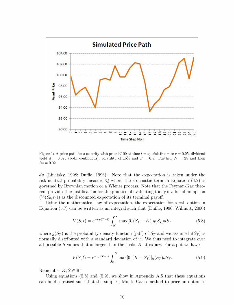
Figure 1: A price path for a security with price R100 at time t = t0, risk-free rate r = 0.05, dividendyield d = 0.025 (both continuous), volatility of 15% and T = 0.5. Further, N = 25 and then∆t = 0.02

du (Linetsky, 1998; Duffie, 1996). Note that the expectation is taken under therisk-neutral probability measure Q where the stochastic term in Equation (4.2) isgoverned by Brownian motion or a Wiener process. Note that the Feyman-Kac theo-rem provides the justification for the practice of evaluating today’s value of an option(Vl(S0, t0)) as the discounted expectation of its terminal payoff.

Using the mathematical law of expectation, the expectation for a call option inEquation (5.7) can be written as an integral such that (Duffie, 1996; Wilmott, 2000)

V (S, t) = e−rT (T−t)∫ ∞K

max[0, (ST −K)]g(ST )dST (5.8)

where g(ST ) is the probability density function (pdf) of ST and we assume ln(ST ) isnormally distributed with a standard deviation of w. We thus need to integrate overall possible S-values that is larger than the strike K at expiry. For a put we have

V (S, t) = e−rT (T−t)∫ K

0

max[0, (K − ST )]g(ST )dST . (5.9)

Remember K,S ∈ R+0

Using equations (5.8) and (5.9), we show in Appendix A.5 that these equationscan be discretised such that the simplest Monte Carlo method to price an option is

10

given by

VMC(S, t) = e−rT (T−t)1

M

M∑i=1

max[0, φ(ST −K)] (5.10)

where ST is attained after N time steps that coincide with the expiry time T . Wecan use either Equation (4.5) or Equation (4.6) to estimate ST . To obtain the MonteCarlo option price, we need to obtain M , ST values. This means we simulate ST , Mtimes to obtain the average option value VMC . Note: N is the number of time stepsand M the number of simulations.

By scrutinising equations (5.10), (4.5) and (4.6) it becomes clear that MC methodsare indeed techniques utilising random numbers and probability to solve problems.It is evident that such an analysis is based on artificially recreating a chance process,running it many times and directly observing the results.

Figure 2 shows 5 price paths generated with Equation (4.5), each having 25 timesteps. Here we have a fixed volatility, interest rate and dividend yield (in the limitas M →∞, all ST ’s will have a normal distribution). If we have a call option with astrike price of 100, Equation (5.10) leads to an option value of R11.02. This is shownin Table 1.

Figure 2: Price paths for a security with price R100 at time t = t0, risk-free rate r = 0.05, dividendyield d = 0.025 (both continuous), volatility of 0.25 and T = 1.0. Further, N = 25 and then∆t = 0.04 and M = 5

In the example above we used a fixed volatility of 25%. However, crucial toobtaining the correct terminal values ST is that the volatilities we use in equations(4.5) and (4.6) are the volatilities obtained from a local volatility surface. We thusneed to understand what we mean by the time stamp in the local volatility σ(S(ti), ti)

11

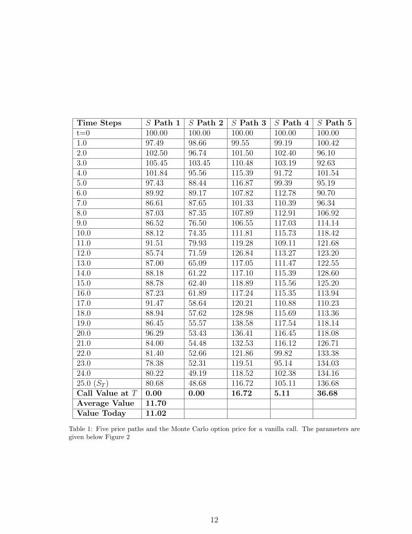
Time Steps S Path 1 S Path 2 S Path 3 S Path 4 S Path 5t=0 100.00 100.00 100.00 100.00 100.001.0 97.49 98.66 99.55 99.19 100.422.0 102.50 96.74 101.50 102.40 96.103.0 105.45 103.45 110.48 103.19 92.634.0 101.84 95.56 115.39 91.72 101.545.0 97.43 88.44 116.87 99.39 95.196.0 89.92 89.17 107.82 112.78 90.707.0 86.61 87.65 101.33 110.39 96.348.0 87.03 87.35 107.89 112.91 106.929.0 86.52 76.50 106.55 117.03 114.1410.0 88.12 74.35 111.81 115.73 118.4211.0 91.51 79.93 119.28 109.11 121.6812.0 85.74 71.59 126.84 113.27 123.2013.0 87.00 65.09 117.05 111.47 122.5514.0 88.18 61.22 117.10 115.39 128.6015.0 88.78 62.40 118.89 115.56 125.2016.0 87.23 61.89 117.24 115.35 113.9417.0 91.47 58.64 120.21 110.88 110.2318.0 88.94 57.62 128.98 115.69 113.3619.0 86.45 55.57 138.58 117.54 118.1420.0 96.29 53.43 136.41 116.45 118.0821.0 84.00 54.48 132.53 116.12 126.7122.0 81.40 52.66 121.86 99.82 133.3823.0 78.38 52.31 119.51 95.14 134.0324.0 80.22 49.19 118.52 102.38 134.1625.0 (ST ) 80.68 48.68 116.72 105.11 136.68Call Value at T 0.00 0.00 16.72 5.11 36.68Average Value 11.70Value Today 11.02

Table 1: Five price paths and the Monte Carlo option price for a vanilla call. The parameters aregiven below Figure 2

12

in these equations. This shows we first of all need the stock price at each time step,i.e., S(ti). We have given some examples in Table 1. But, further to this, we also needthe instantaneous volatility at each time step for each stock price. We can obtainall of this from a three dimensional local volatility surface. We will discuss this insection 6 below.

6. Dupire’s Local Volatility Mapping

Local volatility models are widely used in the finance industry (Engelmann et al.,2009). Whereas stochastic volatility and jump-diffusion models introduce new risksinto the modeling process, local volatility models stay close to the Black-Scholestheoretical framework and only introduce more flexibility to the volatility. This isone of the main reasons of fierce criticism of local volatility models (Ayache et al.,2004). Thus, it is a mistake to interpret local volatility as a complete representationof the true stochastic process driving the underlying asset price. Local volatility ismerely a simplification that is practically useful for describing a price process withnon-constant volatility. A local volatility model is a special case of the more generalstochastic volatility models. That is why these models are also known as “restrictedstochastic volatility models”.

6.1. Dupire’s Formula

The local volatility function σ(S, t) is assumed to be deterministic — it is a de-terministic function of a stochastic quantity St and time. So there is still just onesource of randomness, ensuring that the completeness of the Black-Scholes modelis preserved. Completeness is important, because it guarantees unique prices, thusarbitrage pricing and hedging (Dupire, 1993).

Dupire (1994) was the first to show algebraically that, given prices of European callor put options across all strikes and maturities, we may deduce the volatility functionσ(S, t), which produces those prices via the full Black-Scholes equation (Clark, 2011).Dupire’s insight was that if the spot price follows a risk-neutral random walk and ifno-arbitrage market prices for European vanilla options are available for all strikes andexpiries, then the local volatility σ(S, t) in Equation (4.1) can be extracted analyticallyfrom European option prices (Dupire, 1993). He, unknowingly, applied Gyongy’stheorem (Gyongy, 1986).

Dupire showed that if we have implied or market volatilities, we can calculate thelocal volatilities thereof where (Wilmott (1998) and Clark (2011))

σ2loc(S0, K, τ) =

σ2imp + 2τσimp

∂σimp∂τ

+ 2(r − d)Kτσimp∂σimp∂K(

1 +Kd1√τ∂σimp∂K

)2

+K2τσimp

(∂2σimp∂K2 − d1

√τ

(∂σimp∂K

)2) ,

(6.11)where

d1 =ln (S0/K) +

((r − d) + σ2

imp/2)τ

σimp√τ

,

13

and τ = T − t such that t and S0 are respectively the market date, on which thevolatility smile is observed, and the asset price on that date. Note that Equation(6.11) gives the variance, i.e., σ2. See Kotze et al. (2015) for the derivation.

The main problem is that the implied or traded volatilities are only known atdiscrete strikes K and expiries T . This is why the parameterisation chosen for theimplied volatility surface is very important. If implied volatilities are used directlyfrom the market, the derivatives in Equation (6.11) needs to be obtained numericallyusing finite difference or other well-known techniques. This can still lead to an unsta-ble local volatility surface. Furthermore we will have to interpolate and extrapolatethe given data points unto a surface. Since obtaining the local volatility from thedata involves taking derivatives, the extrapolated implied volatility surface cannot betoo uneven. If it is, this unevenness will be exacerbated in the local volatility surfaceshowing that it is not arbitrage free in these areas.

Kotze et al. (2015) showed that the JSE uses a deterministic functional formfor their ALSI implied volatility surface. This function is quadratic across strikeand exponential across time. This three dimensional function is fitted to tradeddata. They further showed that all derivatives in Equation (6.11) can be obtainedanalytically and the ALSI local volatility surface is easy to calculate and obtain. Theywent further and discussed the DTOP and USDZAR implied volatility surfaces. Thereare no functional forms available and all derivatives in Equation (6.11) needs to becomputed numerically.

6.2. Dupire and Monte Carlo Simulation

The JSE uses Dupire’s formula in Equation (6.11) to convert the implied volatil-ity surfaces for all vanilla options traded on all underlying future contracts to theirrespective local volatility surfaces. The local volatility surfaces are used when exoticoptions are evaluated. Exotics are mostly traded on the ALSI, DTOP and USDZARand some single name futures.

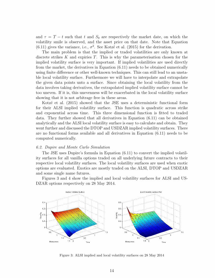
Figures 3 and 4 show the implied and local volatility surfaces for ALSI and US-DZAR options respectively on 28 May 2014.

Figure 3: ALSI implied and local volatility surfaces on 28 May 2014

14

Figure 4: USDZAR implied and local volatility surfaces on 28 May 2014

From Figure 3 we notice that the implied volatility surface does not have a lotof curvature — it is skewed but flat. However, we also see from the local volatilitysurface that it has more curvature. This shows that the local volatility skew is twicethat of the implied volatility skew. Figure 4, shows the USDZAR implied volatilitysurface that has the currency market’s all familiar smile. Here we also show the localvolatility surface with steeper sides.

Continuing with our example: in section 5 and Table 1 we tabulated some pricepaths. We now want to calculate the Dupire local volatility for each stock price ateach time step. This is the local volatility that should then be used in equations (4.5)and (4.6) to obtain the price paths as shown in Table 1.

On a practical note: in equations (4.5) and (4.6) we generate a stock price S(ti)at each time step ti. To apply Equation (6.11) we now say that τ = ti and S(ti) = K.Why? To obtain the local volatility we step forward in time and at every time stepassume we price an option with an expiry time of T and then τ = T − t0 but in mostcases t0 = 0. Further, Dupire’s equation is given in terms of the strike. It holds forall strikes because K ∈ R+

0 . We then say that S(ti) is a possible strike at time ti andwe have K = S(ti).

In our example, the price paths were shown for a one year time period. TheJSE/FTSE Top 40 index was 44,732 on 28 May 2014. The price paths in Table 1were generated with a fixed volatility of 25%. We thus cannot generate the same pricepaths under a local volatility regime. However, to show the difference between a fixedvolatility and local volatility implementation, we now use the same random numbersas before and we assume that the one year ATM volatility is 25%. So we run thisexperiment and generate 5 price paths under the ALSI local volatility surface. Thenewly generated price paths are shown in Figure 5. The actual numbers are listed inTable 2 and the corresponding local volatilities are listed in Table 3.

Comparing graphs 5 and 2 and Tables 2 and 1 reveal that the stock prices are notthat much different. This is the way it should be because the local volatility does notdiffer that much from the implied volatility. However, even these slight differences,can lead to vastly different exotic option prices and especially, Greeks.

15

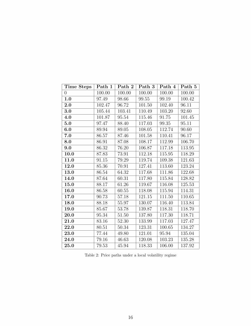
Time Steps Path 1 Path 2 Path 3 Path 4 Path 50 100.00 100.00 100.00 100.00 100.001.0 97.49 98.66 99.55 99.19 100.422.0 102.47 96.72 101.50 102.40 96.113.0 105.44 103.41 110.49 103.20 92.604.0 101.87 95.54 115.46 91.75 101.455.0 97.47 88.40 117.03 99.35 95.116.0 89.94 89.05 108.05 112.74 90.607.0 86.57 87.46 101.58 110.41 96.178.0 86.91 87.08 108.17 112.99 106.709.0 86.32 76.20 106.87 117.18 113.9510.0 87.83 73.91 112.18 115.95 118.2911.0 91.15 79.29 119.74 109.38 121.6312.0 85.36 70.91 127.41 113.60 123.2413.0 86.54 64.32 117.68 111.86 122.6814.0 87.64 60.31 117.80 115.84 128.8215.0 88.17 61.26 119.67 116.08 125.5316.0 86.58 60.55 118.08 115.94 114.3117.0 90.73 57.18 121.15 111.50 110.6518.0 88.18 55.97 130.07 116.40 113.8419.0 85.67 53.78 139.87 118.31 118.7020.0 95.34 51.50 137.80 117.30 118.7121.0 83.16 52.30 133.99 117.03 127.4722.0 80.51 50.34 123.31 100.65 134.2723.0 77.44 49.80 121.01 95.94 135.0424.0 79.16 46.63 120.08 103.23 135.2825.0 79.53 45.94 118.33 106.00 137.92

Table 2: Price paths under a local volatility regime

16

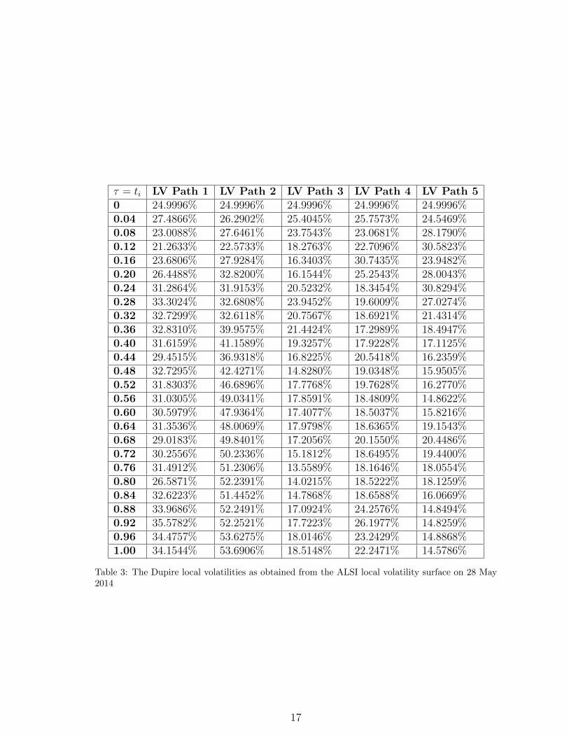
τ = ti LV Path 1 LV Path 2 LV Path 3 LV Path 4 LV Path 50 24.9996% 24.9996% 24.9996% 24.9996% 24.9996%0.04 27.4866% 26.2902% 25.4045% 25.7573% 24.5469%0.08 23.0088% 27.6461% 23.7543% 23.0681% 28.1790%0.12 21.2633% 22.5733% 18.2763% 22.7096% 30.5823%0.16 23.6806% 27.9284% 16.3403% 30.7435% 23.9482%0.20 26.4488% 32.8200% 16.1544% 25.2543% 28.0043%0.24 31.2864% 31.9153% 20.5232% 18.3454% 30.8294%0.28 33.3024% 32.6808% 23.9452% 19.6009% 27.0274%0.32 32.7299% 32.6118% 20.7567% 18.6921% 21.4314%0.36 32.8310% 39.9575% 21.4424% 17.2989% 18.4947%0.40 31.6159% 41.1589% 19.3257% 17.9228% 17.1125%0.44 29.4515% 36.9318% 16.8225% 20.5418% 16.2359%0.48 32.7295% 42.4271% 14.8280% 19.0348% 15.9505%0.52 31.8303% 46.6896% 17.7768% 19.7628% 16.2770%0.56 31.0305% 49.0341% 17.8591% 18.4809% 14.8622%0.60 30.5979% 47.9364% 17.4077% 18.5037% 15.8216%0.64 31.3536% 48.0069% 17.9798% 18.6365% 19.1543%0.68 29.0183% 49.8401% 17.2056% 20.1550% 20.4486%0.72 30.2556% 50.2336% 15.1812% 18.6495% 19.4400%0.76 31.4912% 51.2306% 13.5589% 18.1646% 18.0554%0.80 26.5871% 52.2391% 14.0215% 18.5222% 18.1259%0.84 32.6223% 51.4452% 14.7868% 18.6588% 16.0669%0.88 33.9686% 52.2491% 17.0924% 24.2576% 14.8494%0.92 35.5782% 52.2521% 17.7223% 26.1977% 14.8259%0.96 34.4757% 53.6275% 18.0146% 23.2429% 14.8868%1.00 34.1544% 53.6906% 18.5148% 22.2471% 14.5786%

Table 3: The Dupire local volatilities as obtained from the ALSI local volatility surface on 28 May2014

17

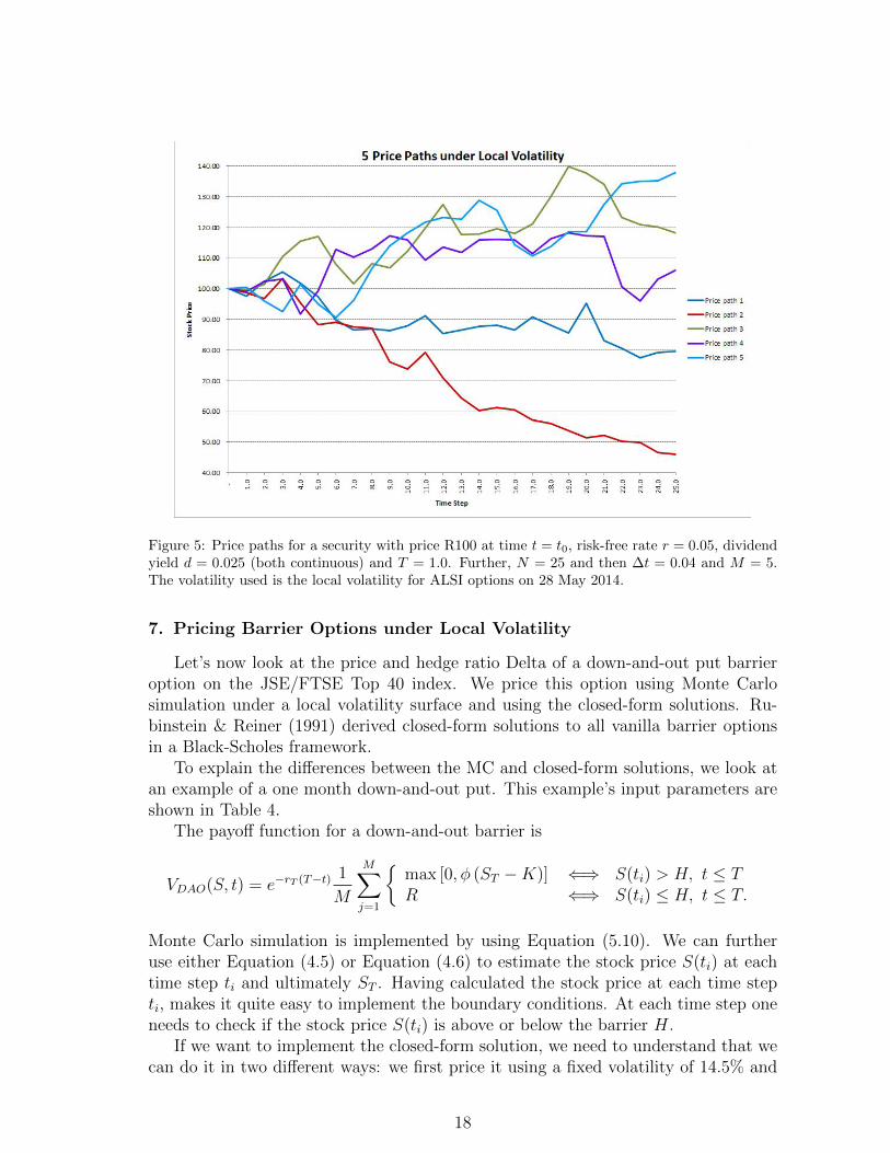
Figure 5: Price paths for a security with price R100 at time t = t0, risk-free rate r = 0.05, dividendyield d = 0.025 (both continuous) and T = 1.0. Further, N = 25 and then ∆t = 0.04 and M = 5.The volatility used is the local volatility for ALSI options on 28 May 2014.

7. Pricing Barrier Options under Local Volatility

Let’s now look at the price and hedge ratio Delta of a down-and-out put barrieroption on the JSE/FTSE Top 40 index. We price this option using Monte Carlosimulation under a local volatility surface and using the closed-form solutions. Ru-binstein & Reiner (1991) derived closed-form solutions to all vanilla barrier optionsin a Black-Scholes framework.

To explain the differences between the MC and closed-form solutions, we look atan example of a one month down-and-out put. This example’s input parameters areshown in Table 4.

The payoff function for a down-and-out barrier is

VDAO(S, t) = e−rT (T−t)1

M

M∑j=1

{max [0, φ (ST −K)] ⇐⇒ S(ti) > H, t ≤ TR ⇐⇒ S(ti) ≤ H, t ≤ T.

Monte Carlo simulation is implemented by using Equation (5.10). We can furtheruse either Equation (4.5) or Equation (4.6) to estimate the stock price S(ti) at eachtime step ti and ultimately ST . Having calculated the stock price at each time stepti, makes it quite easy to implement the boundary conditions. At each time step oneneeds to check if the stock price S(ti) is above or below the barrier H.

If we want to implement the closed-form solution, we need to understand that wecan do it in two different ways: we first price it using a fixed volatility of 14.5% and

18

Description Input Values

Equity price 44 732.00Strike 44 732.00Barrier 40 258.80Rebate 0.000Number of discrete observations 146.00Current date 28-May-14Maturity date 30-Jun-14Interest Rate (NACA) 6.00%Volatility 14.50%Dividend Yield (NACA) 3.00%Type of option Down and out put

Table 4: Input parameters for a down-and-out-put option on the JSE/FTSE Top 40 index.

secondly we obtain the volatility from the implied volatility surface.The price dynamics of this option is shown in Figure 6 where closed-form is ab-

breviated by CF. The barrier is 90% of the spot level and it is short dated. The pricedynamics between the three methods do not differ much and using the slower MonteCarlo method does not add much value. Figure 6 shows the familiar option profile

Figure 6: Price dynamics for a down-and-out-put.

for a down-and-out put option — the option vanishes if the stock price breaches thebarrier level.

The dynamics of the hedge ratio Delta is shown in Figure 7. Here is where theanswers differ substantially. Far from the barrier all three methods give the same

19

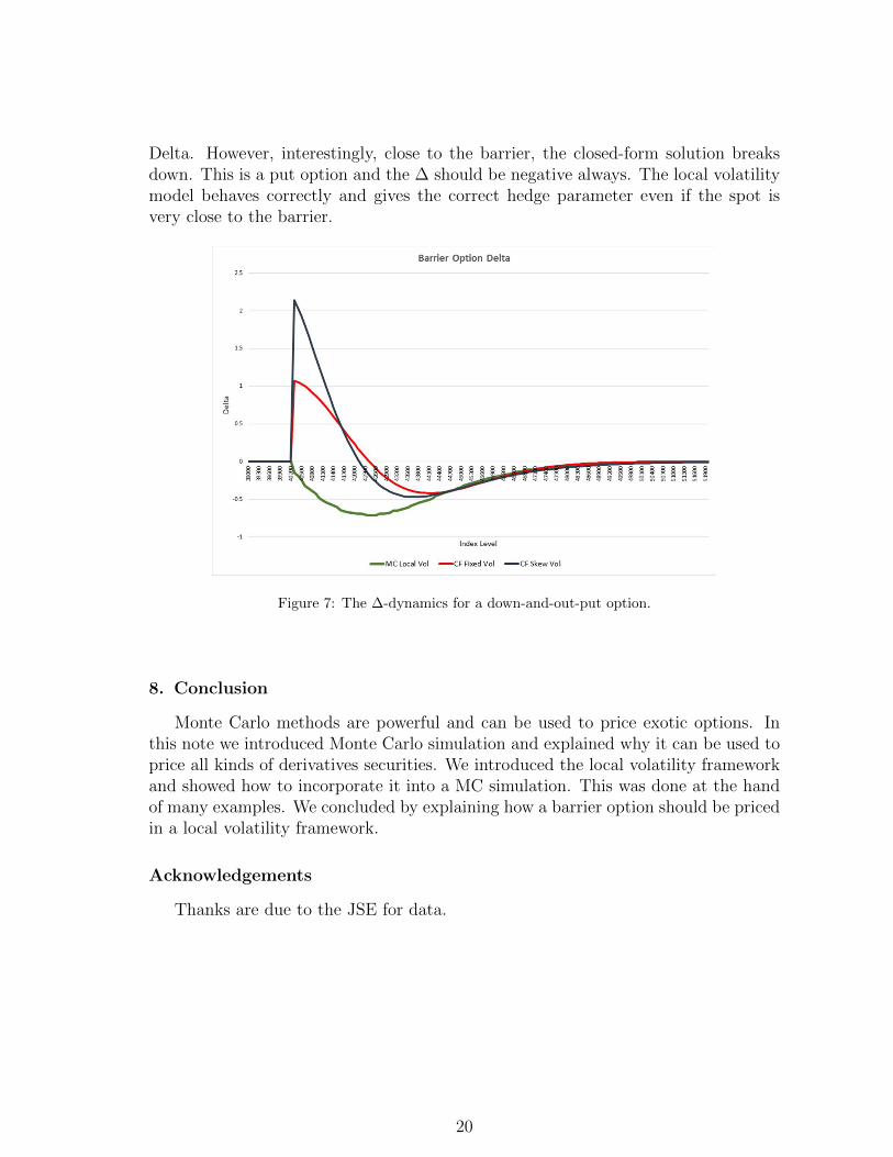
Delta. However, interestingly, close to the barrier, the closed-form solution breaksdown. This is a put option and the ∆ should be negative always. The local volatilitymodel behaves correctly and gives the correct hedge parameter even if the spot isvery close to the barrier.

Figure 7: The ∆-dynamics for a down-and-out-put option.

8. Conclusion

Monte Carlo methods are powerful and can be used to price exotic options. Inthis note we introduced Monte Carlo simulation and explained why it can be used toprice all kinds of derivatives securities. We introduced the local volatility frameworkand showed how to incorporate it into a MC simulation. This was done at the handof many examples. We concluded by explaining how a barrier option should be pricedin a local volatility framework.

Acknowledgements

Thanks are due to the JSE for data.

20

AppendicesA. From Black-Scholes to Discrete Monte Carlo Simulation

A.1. The Feynman-Kac Theorem and ExpectationFourier solved his simplistic heat conduction equation analytically by introducing

Fourier transforms. The extended version is not solved that easily. However, theFeynman-Kac theorem can be used to solve it (Rebonato, 2004). This is possible ifVl(S, t) in Equation (4.3) is twice differentiable and Vl(ST , T ) is the terminal condition.We also have ST being the terminal asset value on the expiry time T . The Feynman-Kac theorem establishes a link between parabolic partial differential equations andstochastic processes or diffusion problems we encounter in finance (Jackel, 2002). Itoffers a method of solving certain PDEs by simulating random paths of a stochasticprocess (Klebaner, 2005; Clark, 2011). If we now let Vl(ST , T ) be the final condition ofour contingent claim at expiry T and, given that the process, S, starts at S0 at initialtime t0, the general solution to this backward parabolic partial differential equationshown in Equation (4.3) is given by

Vl(S0, t0) = EQ[e−

∫ Tt0ruduVl(ST , T )|St0 = S0

], (A.12)

where S, t ∈ R+0 and St is described by the stochastic differential Equation (4.2)

and ru is the instantaneous discount rate applicable for a very short period of timedu (Linetsky, 1998; Duffie, 1996). Note that the expectation is taken under the risk-neutral probability measure Q where the stochastic term in Equation (4.2) is governedby Brownian motion or it is a Wiener process. Note that the Feyman-Kac theoremprovides the justification for the practice of evaluating today’s value of an option(Vl(S0, t0)) as the discounted expectation of its terminal payoff.

In general, if we assume the volatility σ(St, t) is stochastic, Equation (A.12) cannotbe solved analytically. However, the situation is a little more tractable if we assumethe following: the volatility is a deterministic local volatility σ(St, t) and both therisk-free interest rate and dividend yield are deterministic functions. Note that thelocal volatility σ(St, t) should be defined such that it is locally Lipschitz and thatthe Cauchy-Peano local existence theorem8 for ordinary differential equations holds(Duffie, 1996; Hassani, 1991).

To explain this we define B(t) to be the value of a bank account at time t ≥ 0.We assume B(0) = 1 and that the bank account evolves according to the followingdifferential equation

dB(t) = rtB(t)dt, B(0) = 1

where rt is a positive function of time (Brigo & Mercurio, 2001). If we integrate weget

B(t) = exp

(∫ t

0

rudu

).

8Compare the Picard-Lindelof theorem or Picard’s existence theorem as well

21

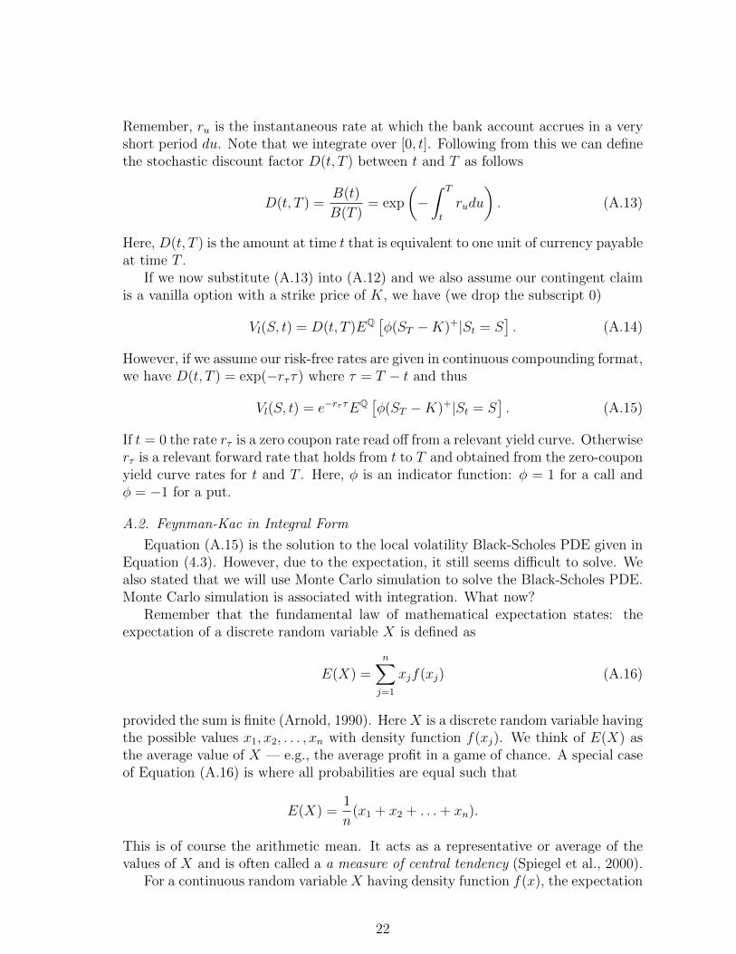
Remember, ru is the instantaneous rate at which the bank account accrues in a veryshort period du. Note that we integrate over [0, t]. Following from this we can definethe stochastic discount factor D(t, T ) between t and T as follows

D(t, T ) =B(t)

B(T )= exp

(−∫ T

t

rudu

). (A.13)

Here, D(t, T ) is the amount at time t that is equivalent to one unit of currency payableat time T .

If we now substitute (A.13) into (A.12) and we also assume our contingent claimis a vanilla option with a strike price of K, we have (we drop the subscript 0)

Vl(S, t) = D(t, T )EQ [φ(ST −K)+|St = S]. (A.14)

However, if we assume our risk-free rates are given in continuous compounding format,we have D(t, T ) = exp(−rττ) where τ = T − t and thus

Vl(S, t) = e−rτ τEQ [φ(ST −K)+|St = S]. (A.15)

If t = 0 the rate rτ is a zero coupon rate read off from a relevant yield curve. Otherwiserτ is a relevant forward rate that holds from t to T and obtained from the zero-couponyield curve rates for t and T . Here, φ is an indicator function: φ = 1 for a call andφ = −1 for a put.

A.2. Feynman-Kac in Integral Form

Equation (A.15) is the solution to the local volatility Black-Scholes PDE given inEquation (4.3). However, due to the expectation, it still seems difficult to solve. Wealso stated that we will use Monte Carlo simulation to solve the Black-Scholes PDE.Monte Carlo simulation is associated with integration. What now?

Remember that the fundamental law of mathematical expectation states: theexpectation of a discrete random variable X is defined as

E(X) =n∑j=1

xjf(xj) (A.16)

provided the sum is finite (Arnold, 1990). Here X is a discrete random variable havingthe possible values x1, x2, . . . , xn with density function f(xj). We think of E(X) asthe average value of X — e.g., the average profit in a game of chance. A special caseof Equation (A.16) is where all probabilities are equal such that

E(X) =1

n(x1 + x2 + . . .+ xn).

This is of course the arithmetic mean. It acts as a representative or average of thevalues of X and is often called a a measure of central tendency (Spiegel et al., 2000).

For a continuous random variable X having density function f(x), the expectation

22

of X is defined as

E(X) =

∫ ∞−∞

xf(x)dx (A.17)

where x ∈ R and provided the integral is finite or converges absolutely (Arnold, 1990).Using the mathematical law of expectation, the expectation for a call option in

Equation (A.15) can be written as an integral such that (Duffie, 1996; Wilmott, 2000)

V (S, t) = e−rT (T−t)∫ ∞K

max[0, (ST −K)]g(ST )dST (A.18)

where g(ST ) is the probability density function (pdf) of ST and we assume ln(ST ) isnormally distributed with a standard deviation of w. We thus need to integrate overall possible S-values that is larger than the strike K at expiry. For a put we have

V (S, t) = e−rT (T−t)∫ K

0

max[0, (K − ST )]g(ST )dST . (A.19)

Remember K,S ∈ R+0

Under the assumption of a constant volatility and interest rate, the integrals inEquations (A.18) and (A.19) can be solved analytically leading to the well-knownBlack-Scholes option pricing formulae for calls and puts. However, if we just relaxthe assumptions of constant volatility and constant interest rate slightly and assumethat these two quantities are deterministic (but not constant), the integral cannot becalculated analytically anymore. The integral needs to be solved numerically.

The integral can be solved using Monte Carlo simulation. However, in order todo that, we need to know how ST behaves or what the dynamics of ST is. This isnow quite simple because we know that equations (A.12) and (A.15) are only validif the asset price dynamics are described by the stochastic differential equation givenin (4.2).

A.3. Integrating the SDEThe stochastic differential equation given in Equation (4.2) describes the dynamics

of our stochastic asset price S. However, we understand this SDE much better if wemake a change of variables. Remember, we stated that ln(ST ) is normally distributedso let’s re-write (4.2) in terms of ln(S). Let’s consider the process Xt = f(St) definedby f(x) = ln(x) (Clark, 2011). Remember that f ′(x) = 1/x and f ′′(x) = −x−2. Asimple application of Ito’s lemma gives

dXt = (rt − dt)dt+ σ(St, t)dWt −1

2σ2(St, t)dt. (A.20)

Remember, Wt is a standard Brownian motion and as such dWt = ε√dt where

ε ∼ N(0, 1), N(0, 1) being a standardised normal distribution. Following from this,Equation (A.20) can be integrated to give

XT = X0 +

((rT − dT )− 1

2σ2(ST , T )

)T + σ(ST , T )ε

√T . (A.21)

23

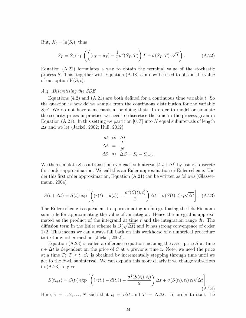
But, Xt = ln(St), thus

ST = S0 exp

(((rT − dT )− 1

2σ2(ST , T )

)T + σ(ST , T )ε

√T

). (A.22)

Equation (A.22) formulates a way to obtain the terminal value of the stochasticprocess S. This, together with Equation (A.18) can now be used to obtain the valueof our option V (S, t).

A.4. Discretising the SDE

Equations (4.2) and (A.21) are both defined for a continuous time variable t. Sothe question is how do we sample from the continuous distribution for the variableST ? We do not have a mechanism for doing that. In order to model or simulatethe security prices in practice we need to discretise the time in the process given inEquation (A.21). In this setting we partition [0, T ] into N equal subintervals of length∆t and we let (Jackel, 2002; Hull, 2012)

dt ≈ ∆t

∆t =T

NdS ≈ ∆S = St − St−1.

We then simulate S as a transition over each subinterval [t, t+∆t] by using a discretefirst order approximation. We call this an Euler approximation or Euler scheme. Un-der this first order approximation, Equation (A.21) can be written as follows (Glasser-mann, 2004)

S(t+ ∆t) = S(t) exp

[((r(t)− d(t))− σ2(S(t), t)

2

)∆t+ σ(S(t), t)εt

√∆t

]. (A.23)

The Euler scheme is equivalent to approximating an integral using the left Riemannsum rule for approximating the value of an integral. Hence the integral is approxi-mated as the product of the integrand at time t and the integration range dt. Thediffusion term in the Euler scheme is O(

√∆t) and it has strong convergence of order

1/2. This means we can always fall back on this workhorse of a numerical procedureto test any other method (Jackel, 2002).

Equation (A.23) is called a difference equation meaning the asset price S at timet + ∆t is dependent on the price of S at a previous time t. Note, we need the priceat a time T ; T ≥ t. ST is obtained by incrementally stepping through time until weget to the N -th subinterval. We can explain this more clearly if we change subscriptsin (A.23) to give

S(ti+1) = S(ti) exp

[((r(ti)− d(ti))−

σ2(S(ti), ti)

2

)∆t+ σ(S(ti), ti) εt

√∆t

].

(A.24)Here, i = 1, 2, . . . , N such that ti = i∆t and T = N∆t. In order to start the

24

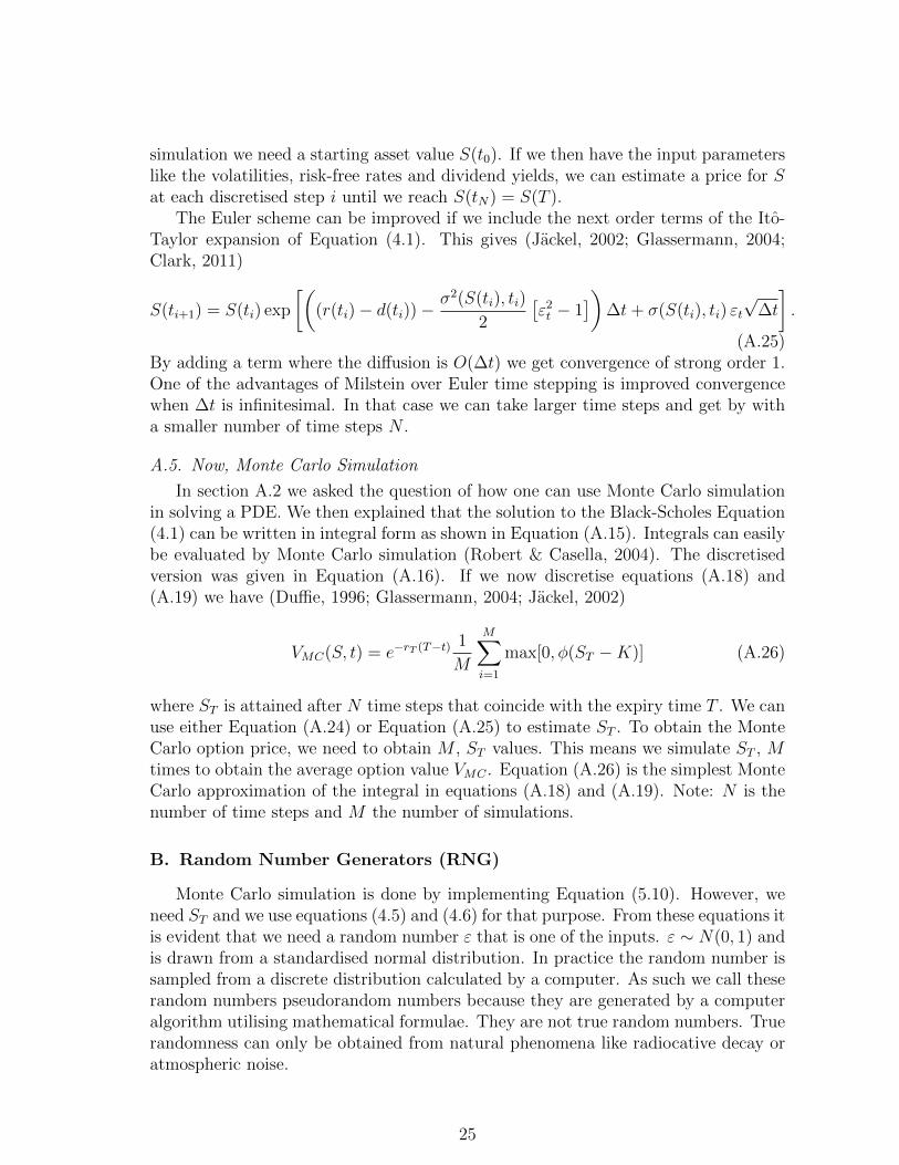
simulation we need a starting asset value S(t0). If we then have the input parameterslike the volatilities, risk-free rates and dividend yields, we can estimate a price for Sat each discretised step i until we reach S(tN) = S(T ).

The Euler scheme can be improved if we include the next order terms of the Ito-Taylor expansion of Equation (4.1). This gives (Jackel, 2002; Glassermann, 2004;Clark, 2011)

S(ti+1) = S(ti) exp

[((r(ti)− d(ti))−

σ2(S(ti), ti)

2

[ε2t − 1

])∆t+ σ(S(ti), ti) εt

√∆t

].

(A.25)By adding a term where the diffusion is O(∆t) we get convergence of strong order 1.One of the advantages of Milstein over Euler time stepping is improved convergencewhen ∆t is infinitesimal. In that case we can take larger time steps and get by witha smaller number of time steps N .

A.5. Now, Monte Carlo Simulation

In section A.2 we asked the question of how one can use Monte Carlo simulationin solving a PDE. We then explained that the solution to the Black-Scholes Equation(4.1) can be written in integral form as shown in Equation (A.15). Integrals can easilybe evaluated by Monte Carlo simulation (Robert & Casella, 2004). The discretisedversion was given in Equation (A.16). If we now discretise equations (A.18) and(A.19) we have (Duffie, 1996; Glassermann, 2004; Jackel, 2002)

VMC(S, t) = e−rT (T−t)1

M

M∑i=1

max[0, φ(ST −K)] (A.26)

where ST is attained after N time steps that coincide with the expiry time T . We canuse either Equation (A.24) or Equation (A.25) to estimate ST . To obtain the MonteCarlo option price, we need to obtain M , ST values. This means we simulate ST , Mtimes to obtain the average option value VMC . Equation (A.26) is the simplest MonteCarlo approximation of the integral in equations (A.18) and (A.19). Note: N is thenumber of time steps and M the number of simulations.

B. Random Number Generators (RNG)

Monte Carlo simulation is done by implementing Equation (5.10). However, weneed ST and we use equations (4.5) and (4.6) for that purpose. From these equations itis evident that we need a random number ε that is one of the inputs. ε ∼ N(0, 1) andis drawn from a standardised normal distribution. In practice the random number issampled from a discrete distribution calculated by a computer. As such we call theserandom numbers pseudorandom numbers because they are generated by a computeralgorithm utilising mathematical formulae. They are not true random numbers. Truerandomness can only be obtained from natural phenomena like radiocative decay oratmospheric noise.

25

Many pseudorandom number generators have been developed over the past fewdecades. One of the generators used by many practitioners is the Mersenne Twister9

(Jackel, 2002). This algorithm has been implemented in many programming lan-guages like C++ and even VBA10. Another excellent RNG is the Park-Miller algo-rithm with Bays-Durham shuffle (Park & Miller, 1988).

Most RNG generate uniform random numbers. This means these numbers aredrawn from a uniform distribution. However, we need normal random numbers. TheBox-Muller transform is widely used (Jackel, 2002; Glassermann, 2004).

C. Monte Carlo Simulation and Convergence

In general, Monte Carlo methods give us at best a statistical error estimate. AMonte Carlo calculation usually follows the following steps: carry out the same pro-cedure many times, take into account all of the individual results, and summarisethem into an overall approximation to the problem in question. The approximationis usually the average. The numerically exact solution will be approached only as weiterate the procedure more and more times, eventually converging at infinity (Jackel,2002; Glassermann, 2004).

This will be very time consuming so we are not just interested in a method toconverge to the correct answer after an infinite amount of calculation time, but ratherwe wish to have a good approximation quickly. Therefore, once we are satisfied thata particular Monte Carlo method works in the limit, we are naturally interested inits convergence behaviour, or, more specifically, its convergence speed.

Techniques have been developed to reduce the variance of the result and thus toreduce the number of simulations required for a given accuracy. Such techniques arecalled “variance reduction techniques.”

The most widely used techniques are Antithetic Sampling and Control Variates.Jackel (2002) and Glassermann (2004) give very good overviews of these techniques.

9http://www.math.sci.hiroshima-u.ac.jp/~m-mat/MT/emt.html10http://www.math.sci.hiroshima-u.ac.jp/~m-mat/MT/VERSIONS/BASIC/basic.html

26

Bibliography

Andersen, L., & Andreasen, J. (2000). Jump diffusion processees: Volatility smilefitting and numerical methods for option pricing. Review of Derivatives Research,4 , 231–261.

Arnold, S. (1990). Mathematical Statistics . Prentice-Hall.

Ayache, E., Henrotte, P., Nassar, S., & Wang, X. (2004). Can anyone solve the smileproblem? Wilmott Magazine, January , 78–96.

Black, F. (1988). The holes in black-scholes. Risk , 1 , 30–32.

Black, F., & Scholes, M. (1973). The pricing of options and corporate liabilities. TheJournal of Political Economy , 81 , 637–654.

Boas, M. (1983). Mathematical Methods in the Physical Sciences . (2nd ed.). Wiley.

Bouzoubaa, M., & Osserein, A. (2010). Exotic Options and Hybrids: A Guide toStructuring, Pricing and Trading . Wiley Finance.

Boyle, P. (1977). Options: A monte carlo approach. Journal of Financial Economics ,4 , 323–338.

Boyle, P., Broadie, M., & Glasserman, P. (1997). Monte carlo methods for securitypricing. Journal of Economic Dynamics and Control , 21 , 1267–1321.

Brigo, D., & Mercurio, F. (2001). Interest Rate Models: Theory and Practice.Springer.

Broadie, M., & Glasserman, P. (1997). Pricing american-style securities using simu-lation. Journal of Economic Dynamics and Control , 21 , 1323–1352.

Broadie, M., Glassermann, P., & Kou, S. (1997). A continuity correction for discretebarrier options. Mathematical Finance, 7 , 325–348.

Clark, I. (2011). Foreign exchange option pricing . Wiley Finance.

Copeland, B. (2008). The modern history of computing. The Stanford Encyclopediaof Philosophy , Fall . URL: http://plato.stanford.edu/archives/fall2008/

entries/computing-history/.

Dasgupta, S. (2014). It Began with Babbage: The Genesis of Computer Science.Oxford University Press.

Derman, E., & Kani, I. (1994). Riding on a smile. RISK Magazine, 1 , 32–39.

Duffie, D. (1996). Dynamic Assep Pricing Theory . Princeton University Press.

Dupire, B. (1993). Pricing and hedging with smiles. Paribas Capital Markets Swapsand Options Research Team, (pp. 1–9).

27

Dupire, B. (1994). Pricing with a smile. RISK Magazine, 1 , 18–20.

Dyson, G. (2012). Turing’s Cathedral: The Origins of the Digital Universe. Vintage.

Engelmann, B., Fengler, M., & Schwendner, P. (2009). Better than its reputation: Anempirical hedging analysis of the local volatility model for barrier options. Journalof Risk , 12 , 53–77.

Glassermann, P. (2004). Monte Carlo Methods in Financial Engineering . Springer.

Gyongy, I. (1986). Mimicking the one-dimensional marginal distributions of processeshaving an Ito differential. Probability Theory and Related Fields , 71 , 501–516.

Haigh, T. (2015). The tears of Donald Knuth. Communications of the ACM , 58 ,40–44.

Haigh, T., Priestley, M., & Rope, C. (2014). Engineering “the miracle of the ENIAC”:Implementing the modern code paradigm. IEEE Annals of the History of Comput-ing , April-June, 1058–6180.

Harras, G. (2012). On the emergence of volatility, return autocorrelation and bub-bles in Equity markets . Ph.D. thesis ETH Zurich. http://www.er.ethz.ch/

publications/GeorgesHarras_PhD-Thesis.pdf.

Hassani, S. (1991). Foundations of Mathematical Physics . Prentice-Hall.

Haug, E. (2007). The Complete Guide to Option Pricing Formulas . McGraw-Hill.

Hull, J. (2012). Options, Futures, and other Derivatives . Pearson.

Istrail, S., & Marcus, S. (2013). Alan Turing and John von Neumann - their brainsand their computers. Membrane Computing: Lecture Notes in Computer Science,7752 , 26–35.

Jackel, P. (2002). Monte Carlo Methods in Finance. John Wiley & Sons.

Klebaner, F. (2005). Introduction to Stochastic Calculus With Applications, SecondEdition. London, UK: Imperial College Press.

Kotze, A. (2003). Black-scholes or black holes? The South African Financial MarketsJournal , 2 , 8–12.

Kotze, A., & Oosthuizen, R. (2013). JSE exotic can-do options: determining initialmargins. The South African Financial Markets Journal , 17 . URL: http://www.financialmarketsjournal.co.za/17thedition/jseequity.htm.

Kotze, A., Oosthuizen, R., & Pindza, E. (2015). Implied and local volatility surfacesfor south african index and foreign exchange options. Journal of Risk and FinancialManagement , 8 , 43–82. URL: http://www.mdpi.com/1911-8074/8/1/43.

28

Lagnado, R., & Osher, S. (1997). Reconciling differences. RISK Magazine, 1 , 79–83.

Linetsky, V. (1998). The path integral approach to financial modeling and optionspricing. Computational Economics , 11 , 129–163.

Longstaff, F., & Schwartz, E. (1991). Valuing american options by simulation: Asimple least-squares approach. The Review of Financial Studies , 14 , 113–147.

McCauley, J. (2013). Stochastic Calculus and Differential Equations for Physics andFinance. Cambridge.

McLeish, D. (2005). Monte Carlo Simulation & Finance. Wiley Finance.

Merton, R. (1973). Theory of rational option pricing. Bell Journal of Economics andManagement Science, 4 , 141–183.

Metropolis, N., & Ulam, S. (1949). The Monte Carlo method. Journal of the AmericanStatistical Association, 44 , 335–341.

Morrison, F. (2008). The Art of Modeling Dynamic Systems: Forecasting for Chaos,Randomness and Determinism. Dover Publications.

Narasihan, T. N. (1999). Fourier’s heat conduction equation: History, influence, andconnections. Reviews of Geophysics , 37 , 151–172.

Park, S., & Miller, K. (1988). Random number generators: Good ones are hard tofind. Communications of the ACM , 31 , 1192–1201.

Rebonato, R. (2004). Volatility and Correlation: the Perfect Hedger and the Fox,2ndEdition. John Wiley & Sons.

Reif, F. (2008). Fundamentals of Statistical and Thermal Physics . Springer Texts inStatistics. Waveland Pr Inc.

Rich, D. (1994). The mathematical foundations of barrier option-pricing theory.Advances in Futures and Options Research, 7 , 267–312.

Robert, C., & Casella, G. (2004). Monte Carlo Statistical Methods . Springer Textsin Statistics. Springer.

Rubinstein, M. (1994). Implied binomial trees. Journal of Finance, 49 , 771–818.

Rubinstein, M., & Reiner, E. (1991). Breaking down barriers. Risk , September .

Sornette, D. (2014). Physics and financial economics (1776-2014): Puzzles, Ising andagent-based models. arXiv [q-fin.GN] , 1404.0243 . URL: http://arxiv.org/abs/1404.0243.

Spiegel, M., Schiller, J., & Srinivasan, R. (2000). Probability and Statistics . Schaum’sOutlines (2nd ed.). McGraw-Hill.

29

Steinhauser, M. (2013). Computer Simulation in Physics and Engineering . DeGreyter.

Swade, D. (2005). The construction of charles babbage’s difference engine no. 2. IEEEAnnals of the History of Computing , July-September , 70–88.

Tan, C. (2010). Demystifying Exotic Products: Interest Rates, Equities and ForeignExchange. John Wiley & Sons.

Turing, A. (1936). On computable numbers, with an application to the Entschei-dungsproblem. Proceedings of the London Mathematical Society , 42 , 230–265.

Weber, N. (2011). Implementing Models of Financial Derivatives: Object OrientedApplications with VBA. Wiley Finance.

de Weert, F. (2008). Exotic Options Trading . Wiley Finance.

Wilmott, P. (1998). Derivatives . John Wiley and Sons.

Wilmott, P. (2000). Quantitative Finance. John Wiley & Sons.

Zhang, P. (1998). Exotic Options: A guide to second generation options . (2nd ed.).World Scientific.

30