The Approximate Rank of a Matrix and its Algorithmic Applications ∗

Noga Alon † Troy Lee ‡ Adi Shraibman § Santosh Vempala ¶

December 21, 2013

Abstract

We study the ε-rank of a real matrix A, defined for any ε > 0 as the minimum rank overmatrices that approximate every entry of A to within an additive ε. This parameter is connectedto other notions of approximate rank and is motivated by problems from various topics includingcommunication complexity, combinatorial optimization, game theory, computational geometry andlearning theory. Here we give bounds on the ε-rank and use them for algorithmic applications.Our main algorithmic results are (a) polynomial-time additive approximation schemes for Nashequilibria for 2-player games when the payoff matrices are positive semidefinite or have logarithmicrank and (b) an additive PTAS for the densest subgraph problem for similar classes of weightedgraphs. We use combinatorial, geometric and spectral techniques; our main new tool is an efficientalgorithm for the following problem: given a convex body A and a symmetric convex body B, finda covering a A with translates of B.

1 Introduction

1.1 Background

A large body of work in theoretical computer science deals with various ways of approximating amatrix by a simpler one. The motivation from the design of approximation algorithms is clear. Whenthe input to a computational problem is a matrix (that may represent a weighted graph, a payoffmatrix in a two-person game or a weighted constraint satisfaction problem), the hope is that it iseasier to solve or approximately solve the computational problem for the approximating matrix, whichis simpler. If the notion of approximation is suitable for the problem at hand, then the solution willbe an approximate solution for the original input matrix as well.

A typical example of this reasoning is the application of cut decomposition and that of regulardecomposition of matrices. The cut-norm of a matrix A with a set of rows R and a set of columns Cis

maxS⊂R,T⊂T

|∑

i∈S,j∈TAij |.

∗A preliminary version of this paper appeared in Proc. STOC 2013†Schools of Mathematics and Computer Science, Sackler Faculty of Exact Sciences, Tel Aviv University, Tel Aviv

69978, Israel. Email: nogaa@tau.ac.il. Research supported in part by an ERC Advanced grant, by a USA-Israeli BSFgrant, and by the Hermann Minkowski Minerva Center for Geometry in Tel Aviv University.‡Centre for Quantum Technologies, Singapore. Email: troyjlee@gmail.com§School of Computer Science, Academic College of Tel-Aviv Yaffo, Israel. Email: adish@mta.ac.il¶School of Computer Science and ARC, Georgia Tech, Atlanta 30332. Email: vempala@gatech.edu. Supported in

part by the NSF and by a Raytheon fellowship.

1

A cut matrix B(S, T ; r) is a matrix B for which Bij = r iff i ∈ S, j ∈ T and Bij = 0 otherwise. Friezeand Kannan showed that any n by m matrix B with entries in [−1, 1] can be approximated by a sumof at most 1

ε2cut matrices, in the sense that the cut norm of the difference between B and this sum

is at most εmn. Such an approximation can be found efficiently and leads to several approximationalgorithms for dense graphs—see [19]. Similar approximations of matrices can be given using variantsof the regularity lemma of Szemeredi. These provide a more powerful approximation at the expenseof increasing the complexity of the approximating matrix, and supply approximation algorithms foradditional problems see [6, 18, 7].

All these methods, however, deal with global properties, as the approximation obtained by allthese variants of the regularity lemma are not sensitive to local changes in the matrix. In particular,these methods cannot provide approximate solutions to problems like that of finding an approximateNash equilibrium in a two person game, or that of approximating the maximum possible density of asubgraph on, say,

√n vertices in a given n vertex weighted graph. Motivated by applications of this

type, it is natural to consider a stronger notion of approximation of a matrix, an approximation inthe infinity norm, by a matrix of low rank. This motivates the following definition.

Definition 1.1 For a real n× n matrix A, the ε-rank of A is defined as follows:

ε-rank(A) = minrank(B) : B ∈ <n×n, ‖A−B‖∞ ≤ ε.

We will usually assume that the matrix A has entries in [−1, 1], but the definition holds for anyreal matrix. Define the density norm of a matrix A to be

den(A) = maxx,y∈<n

+

|xTAy|‖x‖1‖y‖1

.

It is easy to verify that the following definition of ε-rank is equivalent to Definition 1.1:

ε-rank(A) = min rank(B) : B ∈ <n×n, den(A−B) ≤ ε.

The investigation of notions of simple matrices that approximate given ones is motivated not onlyby algorithmic applications, but by applications in complexity theory as well. Following Valiant [42]call a matrix A (r, s)-rigid if for any matrix B of the same dimensions as A and rank at most r, A−Bcontains a row with at least s nonzero entries. Here the notion of simple matrix is thus a matrix of lowrank, and the notion of approximation is to allow a limited number of changes in each row. Valiantproved that if an n by n matrix is (Ω(n), nΩ(1))-rigid, then there is no arithmetic circuit of linear sizeand logarithmic depth that computes Ax for any given input x. Therefore, the main problem in thiscontext (which is still wide open) is to give an explicit construction of such a rigid matrix.

Another notion that received a considerable amount of attention is the sign-rank of a real matrix.For a matrix A, rank±(A) is defined as the minimum rank over matrices each of whose entries has thesame sign as the corresponding entry in the original matrix. The notion of approximation here refersto keeping the signs of the entries, while the simplicity of the approximating matrix is measured byits rank. The sign rank has played a useful role in the study of the unbounded error communicationcomplexity of Boolean functions (see, e.g., [5, 20] and their references), in establishing lower bounds inlearning theory and in providing lower bounds for the size of threshold-of-majority circuits computinga function in AC0 (see [35]). It is clear that for −1, 1 matrices or matrices with entries of absolutevalue exceeding ε, ε-rank(A) ≥ rank±(A), and simple examples show that in many cases the ε-rank isfar larger than the sign-rank.

2

Another line of work on ε-rank is motivated by communication complexity [15, 30, 34]. The ε-error private-coin communication complexity of a Boolean function is bounded from below by thelogarithm of the ε-rank of the corresponding communication matrix (see [27]). In addition, the ε-error private-coin quantum communication complexity of a Boolean function is bounded from belowby log ε-rank(A)/2 where A is the communication matrix of the function. Using this connection, ithas been proven that for fixed ε the 2n by 2n set-disjointness matrix has ε-rank 2Θ(

√n), using the

quantum protocol of Aaronson and Ambainis [1] for disjointness, and Razborov’s lower bound for theproblem (see [34], where there is a lower bound for the trace-norm of any matrix that ε-approximatesthe disjointness matrix restricted to the sets of size n/4.) In another work, Lee and Shraibman [28]have given algorithmic bounds on ε-rank via the γ2 norm. The γ2-norm of a real matrix A, denoted byγ2(A), is the minimum possible value of the product c(X)c(Y ), where c(Z) is the maximum `2-norm ofa column of a matrix Z, and the minimum is taken over all factorizations of A of the form A = XtY .For a sign matrix A and for α ≥ 1, let γα2 (A) denote the minimum possible value of γ2(B), where Branges over all matrices of the same dimension as A that satisfy 1 ≤ Aij ·Bij ≤ α for all admissible i, j.Let rankα(A) denote the minimum possible rank of such a matrix B. Note that for α = 1 + ε this is(roughly) the ε/2-rank of A. In [28] it is shown that rankα(A) and γα2 (A) are polynomially related forany sign matrix A, up to a poly-logaritmic factor in the dimension of A. Since γα2 (A) can be computedefficiently using semi-definite programming, this provides a (rough) approximation algorithm for theε-rank of a given sign matrix.

For the special case of the n by n identity matrix the ε-rank has been studied and provided severalapplications. In [2] it is shown that it is at least Ω( logn

ε2 log(1/ε)) and at most O( logn

ε2). This is used in

[2] to derive several applications in geometry, coding theory, extremal finite set theory and the studyof sample spaces supporting nearly independent random variables. See also [11] for a more recentapplication of the lower bound (for the special case ε < 1/

√n) in combinatorial geometry and in the

study of locally correctable codes over real and complex numbers.The notion of the ε-rank of a matrix is also related to learning and to computational geometry.

Indeed, the problem of computing the ε-rank of a given n by n matrix A is equivalent to the geometricproblem of finding the minimum possible dimension of a linear subspace of Rn that intersects thealigned cubes of edge length 2ε centered at the columns of A. In learning, the problem of learning withmargins, the fat-shattering dimension of a family of functions and the problem of learning functionsapproximately are all related to this notion (see e.g., [4] and the references therein).

The focus of our paper is algorithmic applications of ε-rank; we state our results in the next section.

1.2 Results

Our results are divided into three related topics: bounds on the ε-rank, algorithmic applications, andefficient covering of one convex body by another.

Bounds on approximate rank. We begin with bounds on the ε-rank. A well known result ofForster [20] asserts that the sign-rank of any n by n Hadamard matrix H is at least Ω(

√n). This

clearly implies the same lower bound for the ε-rank of any such matrix for any ε < 1. Using theapproximate γ2 norm, Linial et al. [29] further show that ε-rank(H) ≥ (1− 2ε)n. The following givesa slightly stronger estimate, which is tight.

Theorem 1.2 For any n× n Hadamard matrix H and any 0 < ε < 1, ε-rank(H) ≥ (1− ε2)n.

Next we show a lower bound on the approximate rank of a random d-regular graph. Let AG denotethe adjacency matrix of a graph G, and AG denote the “signed” adjacency matrix where the (i, j)

3

entry is 1 for an edge and −1 for a non-edge. We show, in fact, a stronger statement that for a randomd-regular graph the sign rank of AG is Ω(d).

A closely related result was shown by Linial and Shraibman [30]. Similarly to the sign rank, defineγ∞2 (A) as the minimum γ2 norm of a matrix that has the same sign pattern as A and all entries atleast 1 in magnitude. It is known that rank±(A) = O(γ∞2 (A) log(mn)) [12] and also that the sign rankcan be exponentially smaller than γ∞2 [14, 40]. Linial and Shraibman show that γ∞2 (AG) = Ω(

√d) for

a random d-regular graph, which also implies an Ω(d) lower bound on the ε-approximate rank for anyconstant ε < 1/2.

Our proof is different from these γ2 techniques and relies, as in previous lower bounds on the signrank [5], on Warren’s theorem from real algebraic geometry [44].

Theorem 1.3 For almost all d-regular graphs G on n vertices rank±(AG) = Ω(d) for the adjacencymatrix of G.

By “almost all” we mean that the fraction of d-regular graphs on n vertices for which the statementholds tends to 1 as n tends to infinity. Note that as AG = 2AG − J , where J is the all ones matrix,this result also implies that ε-rank(AG) = Ω(d) for any ε < 1/2. The lower bound here is tight forε-rank up to a log n factor: it follows from results in [29, 28] that for any fixed ε bounded away fromzero the ε-rank of AG for every d-regular graph on n vertices is O(d log n). The lower bound is tightfor sign rank, as a result of [5] implies that the sign rank is bounded by the maximal number of signchanges in each row.

The ε-rank of any positive semidefinite matrix can be bounded from above as stated in the nexttheorem. The theorem follows via a direct application of the Johnson-Lindenstrauss lemma [25].

Theorem 1.4 For a symmetric positive semi-definite n× n matrix A with |Aij | ≤ 1, we have

ε-rank(A) ≤ 9 log n

ε2 − ε3.

Note that this is nearly tight, by the above mentioned lower bound for the ε-rank of the identitymatrix.

The last theorem can be extended to linear combinations of positive semi-definite (=PSD) matrices.

Corollary 1.5 Let A =∑m

i=1 αiBi where |αi| ≤ 1 are scalars and Bi are n × n PSD matrices withentries at most 1 in magnitude. Then

ε-rank(A) ≤ Cm2 log n

ε2

for an absolute constant C.

Algorithmic applications. The notion of ε-rank and the bounds above have algorithmic applica-tions. The high-level idea is that we can replace the input matrix of a given instance by another thatapproximates it in every entry and has lower rank.

For a 2-player game specified by two payoff matrices A,B, a fundamental problem is computing anapproximate ε-Nash equilibrium of the game (we define this precisely in Section 4.1). Since changingany entry of a payoff matrix can affect the payoff to a player by at most ε, the ε-rank is a verynatural notion in this context. Lipton et al. [31] showed that an ε-Nash for any 2-player game canbe computed in time nO(logn/ε2) and it has been an important open question to determine whether

4

this problem has a PTAS (i.e., an algorithm of complexity of nf(ε)). Our result establishes a PTASwhen A+B is PSD or when A+B has ε-rank O(log n) (and we are given an ε-approximating matrixC of A + B with rank O(log n)), where A and B are the payoff matrices of the game. Note thatthe special case when A + B = 0 corresponds to zero-sum games, a class for which the exact Nashequilibrium can be computed using linear programming. The setting of A + B having constant rankwas investigated by Kannan and Theobald [26], who gave a PTAS for the case when the rank is a

constant. Their algorithm has running time npoly(d,1/ε); ours has complexity [O(1/ε)]dpoly(n), givinga PTAS for ε-rank d = O(log n).

Theorem 1.6 Let A,B ∈ [−1, 1]n×n be the payoff matrices of a 2-player game. If A + B is positivesemidefinite, then an ε-Nash equilibrium of the game can be computed by a deterministic algorithmusing poly(n) space and time

nO(log(1/ε)/ε2)

i.e., there is a PTAS to compute an ε-Nash equilibrium.

The above theorem can be recovered by a similar algorithm using the γ2-norm approach.The next theorem is more general (the γ2 approach seems to achieve only a weaker bound of

(n/ε)O(d) here).

Theorem 1.7 Let A,B ∈ [−1, 1]n×n be the payoff matrices of a 2-player game. Suppose (ε/2)-rank(A + B) = d and suppose we have a matrix C of rank d satisfying ‖A + B − C‖∞ ≤ ε/2. Then,an ε-Nash equilibrium of the game can be computed in time(

1

ε

)O(d)

poly(n).

Note that in particular if the rank of A+B is O(log n) we can simply take C = A+B and get apolynomial-time algorithm.

Our second application is to finding an approximately densest bipartite subgraph, a problem thathas thus far evaded a PTAS even in the dense setting. In fact, there are hardness results indicating thateven the dense case is hard to approximate to within any constant factor, see [3]. Here we observe thatwe can efficiently compute a good additive approximation for the special case that the input matrixhas a small ε-rank (assuming we are given an approximating matrix of low rank). For a matrix A withentries in [0, 1] and subsets S, T of rows and columns, let AS,T be the submatrix induced by S and T .The density of the submatrix AS,T is

density(AS,T ) =

∑i∈S,j∈T Aij

|S||T |

the average of the entries of the submatrix.

Theorem 1.8 Let A be an n × n real matrix with entries in [0, 1]. Then for any integer 1 ≤ k ≤ n,there is a deterministic algorithm to find subsets S, T of rows and columns with |S| = |T | = k s.t.,

density(AS,T ) ≥ max|U |=|V |=k

density(AU,V )− ε.

Its time complexity is bounded by nO(log(1/ε)/ε2) if A is PSD and by(

1ε

)O(d)poly(n) where d = (ε/2)-rank(A)

(and we are given an ε/2-approximation of rank d).

5

Note that this is a bipartite version of the usual densest subgraph problem in which the objectiveis to find the density of the densest subgraph on (say) 2k vertices in a a given (possibly weighted)input graph. It is easy to see that the answers to these two problems can differ by at most a factorof 2, and as the best known polynomial time approximation algorithm for this problem, given in [13],only provides an O(n1/4+o(1))-approximation for an n-vertex graph, this bipartite version also appearsto be very difficult for general graphs.

Covering convex bodies. Our results for general matrices are based on an algorithm to efficientlyfind a near-optimal cover of a convex body A by translates of another convex body B. We state thisresult here as it seems to be of independent interest. Let N(A,B) denote the minimum number oftranslates of B required to cover A. It suffices for the algorithm that an input convex body is specifiedby a membership oracle, along with bounds on its inscribing and circumscribing ball radii and a pointinside the body [23]. In the applications in this paper, the bodies will in fact be explicit polytopes.

Theorem 1.9 For any convex body A and any centrally symmetric convex body B in <d, a cover ofA using translates of B of size N(A,B)2O(d) can be enumerated by a deterministic algorithm usingeither

1. N(A,B)2O(d) time and 2O(d) space, or

2. N(A,B)O(d)d time and poly(d) space.

Although we do not prove it here, we expect that the theorem can be extended to asymmetricconvex bodies1.

1.3 Organization

The rest of the paper is organized as follows. In Section 2 we describe lower and upper bounds for theε-rank of a matrix, presenting the proofs of Theorems 1.2, 1.3, 1.4 and Corollary 1.5. In Section 3 wedescribe efficient constructions of ε-nets which are required to derive the algorithmic applications, andprove Theorem 1.9. Section 4 contains the algorithmic applications including the proofs of Theorems1.6, 1.7 and 1.8. The final Section 5 contains some concluding remarks, open problems and plans forfuture extensions.

2 Bounds on ε-rank

2.1 Lower bounds

We start with the proof of Theorem 1.2, which is based on some spectral techniques. For a symmetricm by m matrix A let λ1(A) ≥ λ2(A) ≥ . . . ≥ λm(A) denote its eigenvalues, ordered as above. Weneed the following simple lemma.

Lemma 2.1 (i) Let A be an n by n real matrix, then the 2n eigenvalues of the symmetric 2n by 2nmatrix

B =

(0 AAT 0

)(1)

1In an earlier version of this paper, we incorrectly claimed a poly(d) space bound while achieving time N(A,B)2O(d).Fortunately, this does not affect any of the time complexity bounds, of the covering theorem or of the applications.

6

appear in pairs λ and −λ.(ii) For any two symmetric m by m matrices B and C and all admissible values of i and j

λi+j−1(B + C) ≤ λi(B) + λj(C).

Proof.(i) Let (x, y) be the eigenvector of an eigenvalue λ of B, where x and y are real vectors of length n.Then Ay = λx and ATx = λy. It is easy to check that the vector (x,−y) is an eigenvector of theeigenvalue −λ of B. This proves part (i).(ii) The proof is similar to that of the Weyl Inequalities - c.f., e.g., [22], and follows from the variationalcharacterization of the eigenvalues. It is easy and well known that

λi(B) = minU, dim(U)=m−i+1

maxx∈U,‖x‖=1

xTBx

where the minimum is taken over all subspaces U of dimension m− i+ 1. Similarly,

λj(C) = minW, dim(W )=m−j+1

maxx∈W,‖x‖=1

xTCx.

Put V = U ∩W . Clearly, the dimension of V is at least m− i− j + 2 and for any x ∈ V, ‖x‖ = 1,

xT (B + C)x = xTBx+ xTCx ≤ λi(B) + λj(C).

Therefore, λi+j−1(B + C) is equal to

minZ, dim(Z)=m−i−j+2

maxx∈Z,‖x‖=1

xT (B + C)x ≤ λi(B) + λj(C).

2

Proof. (of Theorem 1.2). Let E be an n by n matrix, ‖E‖∞ ≤ ε so that the rank of H + E is theε-rank of H. Let B and C be the following two symmetric 2n by 2n matrices

B =

(0 HHT 0

), (2)

C =

(0 EET 0

). (3)

Since H is a Hadamard matrix, BTB = B2 is n times the 2n by 2n identity matrix. It follows thatλ2i (B) = n for all i, and by Lemma 2.1, part (i), exactly n eigenvalues of B are

√n and exactly n are

−√n. In particular λn+1(B) = −

√n.

The absolute value of every entry of E is at most ε, and thus the square of the Frobenuis norm ofC is at most 2n2ε2. As this is the trace of CTC, that is, the sum of squares of eigenvalues of C, itfollows that C has at most 2nε2 eigenvalues of absolute value at least

√n. By Lemma 2.1, part (i), this

implies that there are at most ε2n eigenvalues of C of value at least√n and thus λbε2nc+1(C) <

√n.

By Lemma 2.1, part (ii) we conclude that λn+bε2nc+1(B + C) < 0. Therefore B + C has at leastn − bε2nc negative eigenvalues and hence also at least n − bε2nc positive eigenvalues. Therefore itsrank, which is exactly twice the rank of H + E, is at least 2(n− bε2nc), completing the proof. 2

7

Remark: By the last theorem, if ε < 1√n

then the ε-rank of any n by n Hadamard matrix is n. This

is tight in the sense that for any n which is a power of 4 there is an n by n Hadamard matrix withε-rank n− 1 for ε = 1√

n. Indeed, the matrix

H1 =

+1 +1 +1 −1+1 −1 +1 +1+1 +1 −1 +1+1 −1 −1 −1

(4)

is a 4 by 4 Hadamard matrix in which the sum of elements in every row is of absolute value 2. Thus,the tensor product of k copies of this matrix is a Hadamard matrix of order n = 4k in which the sumof elements in every row is in absolute value 2k. We can thus either add or subtract 1

2k= 1√

nto each

element of this matrix and get a matrix in which the sum of elements in every row is 0, that is, asingular matrix.

In a similar vein, we can show that the ε-rank of any n-by-n matrix A with entries in [−1, 1] is atmost n−1 for ε = 6√

n. Indeed, for any such A = (aij) there are, by the main result of [41], δj ∈ −1, 1

so that for every i, |∑n

j=1 aijδj | ≤ 6√n. Fix such δj and define, for each i, εi = (

∑nj=1 aijδj)/n.

Therefore, for every i, |εi| ≤ 6√n

and∑n

j=1(δjaij − εi) = 0, implying that the inner product of the

vector (δ1, δ2, . . . , δn) with any row of the matrix (aij−δjεi) is zero. Since |δjεi| ≤ 6√n

for all admissible

i, j, this shows that the ε-rank of A is at most n− 1, for ε = 6√n

.

A similar reasoning shows that for any n-by-n matrix A with entries aij ∈ [−1, 1], the ε-rank is at

most n − Ω( ε2nlogn). The argument here proceeds as follows. Break the columns of A into k = ε2n

2 logndisjoint subsets of nearly equal size, thus breaking A into k submatrices, each having n rows androughly 2 logn

ε2columns. It suffices to show that the ε-rank of each of these submatrices is at most

one less than the number of its columns. Let A′ be such a submatrix and let p be the number ofits columns. Let δ = (δ1, . . . , δp) be a random vector in −1, 1p. By the the Chernoff-HoeffdingInequality, with positive (and in fact high) probability the inner product of each row of A′ with δ is ofabsolute value at most εp. We can now proceed as before to get a matrix B′ satisfying ‖A′−B′‖∞ ≤ εso that each row of B′ is orthogonal to the vector δ, completing the proof.

Recall that the sign rank, rank±(A), is the minimal rank of a matrix with the same sign patternas A. In [5] it is shown that there are n-by-n sign matrices A for which rank±(A) ≥ n/32, thus forlarger ε (close to 1) we cannot expect that ε-rank(A) ≤ (1− ε2)n for all A.

The proof of Theorem 1.3 is a simple consequence of a known bound of Warren for the number of signpattern of real polynomials. For a sequence P1, P2, . . . , Pm of real polynomials in ` variables, and forx ∈ R` for which Pi(x) 6= 0 for any i, the sign pattern of the polynomials Pi at x is the vector

(sign(P1(x)), sign(P2(x)), . . . , sign(Pm(x))) ∈ −1, 1m.

Let s(P1, P2, . . . , Pm) denote the total number of sign patterns of the polynomials Pi as x ranges overall points of R` in which no Pi vanishes. Note that this is bounded by the number of connectedcomponents of the semi-variety V = x ∈ R` : Pi(x) 6= 0 for all 1 ≤ i ≤ m. In this notation, thetheorem of Warren is the following.

Theorem 2.2 (Warren [44]) Let P1, P2, . . . , Pm be real polynomials in ` variables, each of degree atmost k. Then the number of connected components of V = x ∈ R` : Pi(x) 6= 0 for all 1 ≤ i ≤ mis at most (4ekm/`)`. Therefore, s(P1, P2, . . . , Pm) ≤ (4ekm/`)`.

8

Proof. [of Theorem 1.3] It is easy and well known that for any admissible n and d (with nd even) thenumber of labelled d regular graphs on n vertices is [Θ(n/d)]nd/2. In particular this number is at least(cn/d)nd/2 for some absolute positive constant c. Let us estimate the number of d-regular graphs Gfor which rank±(AG) ≤ r. For any such matrix there are two matrices B and C where B is an n by rmatrix and C is an r by n matrix, so that sgn(BC) = AG, where sgn(A) is the sign function appliedentrywise to A. Thinking about the 2nr entries of the matrices B and C as variables, every entry oftheir product BC is a degree 2 polynomial in these variables. This means that the number of suchadjacency matrices that have sign rank bounded by r is at most the number of sign patterns of n2

polynomials, each of degree 2, in ` = 2nr variables. (It actually suffices to look at half of the entries,as the matrix is symmetric, but this will not lead to any substantial change in the estimate obtained).By Theorem 2.2 this number is at most (

4e2n2

2nr

)2nr

.

For r < c′d for an appropriate absolute positive constant c′ this is exponentially smaller than thenumber of labelled d-regular graphs on n vertices, completing the proof. 2

2.2 Upper bounds

We will use the Johnson-Lindenstrauss (JL, for short) Lemma [25]. The following version is from[9, 43].

Lemma 2.3 Let R be an n × k matrix, 1 ≤ k ≤ n, with i.i.d. entries from N(0, 1/k). For anyx, y ∈ <n with ‖x‖, ‖y‖ ≤ 1,

Pr(|(RTx)T (RT y)− xT y| ≥ ε) < 2e−(ε2−ε3)k/4.

Proof. (of Theorem 1.4). Since A is PSD there is a matrix B so that A = BBT . Let R be a randomn× k matrix with entries from N(0, 1/k). Consider A = BRRTBT .

For two vectors x, y ∈ <n,E(xTRRT y) = xT y

and by the JL Lemma,Pr(|xTRRT y − xT y| ≥ ε) ≤ 2e−(ε2−ε3)k/4.

Setting, say, k = 9 lnn/(ε2 − ε3) we conclude that whp

‖A− A‖∞ ≤ ε.

2

Proof. (of Corollary 1.5). Put

A1 =1∑

αi>0 αi

∑αi>0

αiBi

and

A2 =1∑

αi<0 |αi|∑αi<0

|αi|Bi.

9

Then A1 and A2 are positive semi-definite with entries of magnitude at most 1. We can thus applyTheorem 1.4 to approximate the entries of each of them to within ε

m and obtain the desired result byexpressing A as a linear combination of A1 and A2 with coefficients whose sum of magnitudes is atmost m. 2

We can sometimes combine the Johnson-Lindenstrauss lemma with some information about thenegative eigenvalues and eigenvectors of a matrix to derive nontrivial bounds for its ε-rank. A moreelaborate use of the lemma arises when trying to estimate the ε-rank of the n by n matrix A = (aij)in which aij = +1 for all i ≥ j and aij = −1 otherwise. This matrix, also known as the half-graphmatrix or the greater-than matrix, is motivated by applications in computational complexity as wellas by regularity partitions. It is known that its ε-rank is Ω(log n/(ε2 log(1/ε))) [2] and is also Ω(log2 n)for any ε < 0.99. The latter inequality follows from the result of [21] that γα2 (A) ≥ Ω(log n) for any α,and the known relation between the ε-rank of A and γα2 (A) for α = 1 + Θ(ε).

The best-known upper bound is that for any ε the ε-rank of A is O(log3 n/ε2) where here onecombines the result of [32] that γ2(A) = O(log n) with the the upper bound on approximate rank interms of approximate γ2 norm [28].

To see this directly, consider a decomposition of A first into an upper-triangular matrix and acomplementary lower-triangular matrix. For the upper-triangular 0-1 matrix, we extract the largeblock of all 1 entries, roughly the upper right quarter of the matrix and let A1 be the matrix of thesame dimensions as A with this block as its support. The remaining matrix can be viewed as twoupper-triangular matrices put together, we recursively extract a block of 1’s from each of them andlet A2 be the matrix (of the same dimensions as A) with support equal to these two blocks. Thisprocess clearly terminates after dlog ne steps, giving a decomposition into l = O(log n) matrices. Nowwe notice that for each matrix in the decomposition, upon removing the all-zero rows and columns, weare left with a block-diagonal matrix, with each block consisting entirely of 1’s. It is easy to see thatusing the JL lemma, any such block-diagonal matrix has ε-rank O(logm/ε2) where m is the numberof blocks; all rows of the same block are mapped to the same random vector and so the entry in theapproximate matrix depends only on the block numbers of the indices. We assign a single randomvector to each index i ∈ [n] formed by concatenating the random vectors for each element of thedecomposition, i.e., a random vector from N(0, 1/k)kl. Then the expectation of the inner productof two such indices is 0 or 1 corresponding to the entry, and the probability of deviation from theexpectation of any single entry by an additive tl is at most e−kl(t

2−t3)/4. Using l = O(log n) andsetting t = ε/l, we get a probability of failure bounded by e−k(ε2−ε3)/l. Thus setting k = O(l log n/ε2),we ensure that with high probability, every entry deviates from its expectation by at most ε. Thetotal dimension of the embedding is kl = O(log3 n/ε2).

3 Constructing ε-nets

For a matrix A that has small ε-rank, we will be able to construct small ε-nets to approximate thequadratic form xTAy for any x, y of `1-norm 1 to within additive ε. We describe the constructionof these nets in this section, then apply them to some algorithmic problems in what follows. Theconstruction in the PSD case is more explicit and independent of the input matrix; we describe thisfirst.

Theorem 3.1 Let A = BBT , where A is an n×n positive semidefinite matrix with entries in [−1, 1]and B is n × d. Let ∆ = ∆n = x ∈ Rn, ‖x‖1 = 1, x ≥ 0. There is a finite set S ⊂ <d independent

10

of A,B such that

∀x ∈ ∆, ∃x ∈ S : ‖BTx− x‖∞ ≤ε√d

with |S| = O(1/ε)d. Moreover, S can be computed in time O(1/ε)dpoly(n).

Proof. We note that since the diagonal entries of A are at most 1, every column of BT has 2-normat most 1. For x ∈ ∆, we have y = BTx ∈ [−1, 1]d. Let us classify the entries of y into buckets basedon their magnitude. Let m = dlog(

√d)e and

bj =

∣∣∣∣i :1

2j≤ |yi| ≤

1

2j−1∣∣∣∣

for j = 1, . . .m− 1, and bm = |i : |yi| ≤ 1/2m−1|. Then

m−1∑j=1

bj2−2j ≤ 1.

We call the vector (b1, b2, . . . , bm) the profile of a vector y. Thus, bj ≤ 22j for all j ≤ m.We will now construct an ε-net by discretizing each coordinate to multiples of ε/

√d. If we replace

each coordinate of a vector y by its nearest multiple of ε/√d, then the resulting vector y satisfies

‖y − y‖∞ ≤ε√d

and thus ‖y − y‖ ≤ ε.

We now bound the size of this ε-net. The total number of distinct profiles is(d+m− 1

m− 1

)( < 22d). (5)

For a fixed profile, the number of ways to realize the profile ( by assigning coordinates to each bucket)is (

d

b1

)(d− b1b2

). . .

(d−

∑m−1j=1 bj

bm

)<

log2 d∏i=1

(d

d/2i

). (6)

This last product is bounded by

2d(H(1/2)+H(1/4)+H(1/8)+...+H(1/d)) = 2O(d),

where H(x) = −x log2 x− (1− x) log2(1− x) is the binary entropy function.For each realization of a profile, the maximum size of the ε-net can be bounded as

Πmj=1

( √d

2j−2ε

)bj≤ (

1

ε)dΠm

j=1

( √d

2j−2

)22j

≤ (1

ε)d2O(d). (7)

The product of (5), (6) and (7) is an upper bound on the size of S. Thus, the size of the net is boundedby [O(1/ε)]d as claimed. 2

We prove a similar algorithmic bound for the general case of a rank k matrix, with a set thatdepends on the input matrix.

11

Theorem 3.2 Let A be an n × n matrix with entries in [−1, 1] and (ε/2)-rank(A) = d. There is afinite set S ⊂ <n s.t.

∀x ∈ ∆,∃x ∈ S : ‖Ax−Ax‖∞ ≤ ε

and |S| = O(1/ε)d. Moreover a set of size O(1/ε)d can be computed in time O(1/ε)dpoly(n) given anε/2-approximating matrix of rank d.

This theorem will be proved using a more general statement, Theorem 1.9. For compact sets A,B,let N(A,B) be the minimum number of translates of B required to cover A. The following boundsare well-known via volume arguments (see e.g., Pisier’s book [33]).

Lemma 3.3 1. For a centrally-symmetric convex body K ∈ <d, N(K, εK) ≤(1 + 2

ε

)d.

2. For a convex body A and a centrally-symmetric convex body B, both in <d,

vol(A)

vol(A ∩B)≤ N(A,B) ≤ 3d

vol(A)

vol(B).

3. For compact sets A,B,C ∈ <d, vol(A+ C) ≤ N(A,B)vol(B + C).

Proof. (of Theorem 3.2). We assume that A has rank d (replacing it with its ε/2 approximation, ifneeded, and rescaling to assume that in this approximation too every entry lies in [−1, 1]). Let K bethe intersection of the span of A with [−1, 1]n. Thus K is a d-dimensional convex body. Now let Lbe the intersection of the span of A with [−ε/2, ε/2]n. A cover of K by copies of L would achieve theproperty we need for S. Note that (ε/2)K = L. Therefore,

N(K,L) = N(K,ε

2K) ≤

(1 +

4

ε

)dusing Lemma 3.3, part (1). We can now apply Theorem 1.9 (proved in the next subsection) to completethe proof. 2

3.1 Constructing nearly optimal ε-nets

In this section we prove Theorem 1.9. We begin with the second part, for which the standard latticeZn can be used. For the near optimal cover size and time complexity of the first part, we will needsome additional tools.

Proof. [of Theorem 1.9(2).] Start by finding a parallelopiped P s.t.

P ⊆ A ∩B ⊆ αP

i.e., a sandwiching of A ∩ B by parallelopipeds. It is shown in [8] that α = 4d can be achieved inpolynomial time. Now apply an affine transformation that makes P a unit cube. Tile the resultingA with unit cubes so that every point of A is covered. This covering can be carried out by a simpledepth-first search enumeration starting with any copy of P that intersects A and only exploring copiesof P that intersect A+ P . We prove two facts about this procedure:

1. The set of cubes intersecting A is connected via paths that use only cubes that intersect A+P .

12

2. The total number of cubes explored in the enumeration is bounded by 2d times the number ofcubes that intersect A+ P , which is bounded by O(d)dN(A,B).

To prove the first part, consider the centers of two cubes P1 and P2 that intersect A and the straightline joining these centers. To go from P1 to P2 it suffices to traverse a sequence of cubes that intersectthis line. Since P1, P2 intersect A, they lie in A+ P , and so do their centers. Thus, by convexity, theline joining the centers lies entirely in A + P and therefore the cubes traversed in the path betweenP1 and P2 all intersect A+ P .

For the second part, we note that the set of cubes intersecting A+ P are all contained in A+ 2P .Therefore, using Lemma 3.3(2), their number is at most

vol(A+ 2P )

vol(P )≤ vol(A+ 2A)

vol(P )≤ 3d(4d)d

vol(A)

vol(A ∩B)

≤ (12d)dN(A,B).

This proves the correctness of the DFS enumeration and bounds its time. Finally, we note thatthe space required is bounded by O(d) times the logarithm of the diameter of A+ P (after making Pa cube), which is polynomial in the input specification. 2

Our main tool for the near-optimal covering is an extremal lattice construction by Rogers [36] from1950. The norm defined by a symmetric convex body K is

‖x‖K = infs : x ∈ sK.

For a lattice L ∈ <d, two standard parameters are its shortest nonzero vector and its covering radius.We recall their definitions:

λ1(K,L) = minx∈L\0

‖x‖K

andµ(K,L) = infs : L+ sK = <d.

Theorem 3.4 [36] For any centrally-symmetric convex body K ⊂ <d, there is an d-dimensional latticeL with the following properties:

1. µ(K,L) ≤ 1, i.e., L+K = <d.

2. λ1(K,L) ≥ 2/3.

Using Minkowski’s first theorem on lattices, we have λ1(K,L)d ≤ 2d det(L)/vol(K)) and thereforedet(L) ≥ 3−dvol(K) for Rogers’ extremal lattice. Lattices with covering radius 1 and large determinantwere investigated in the 1950’s in a series of papers by Rogers [36, 37, 38, 39]. The simplest ofthese consists of choosing a random lattice with a fixed determinant. Whp, this already satisfiesvol(K)det(L) = 2O(d). The highest possible determinant for a covering lattice is an open question. The

current best existential result [39] is a covering lattice L for any convex body K with

vol(K)

det(L)= dO(log log d).

Rogers’ proof of Theorem 3.4 is algorithmic and can be used to compute a basis of an extremallattice. We include a proof here for completeness along with an explicit algorithm and complexityanalysis.

13

Theorem 3.5 [36] For any convex body K in <d given by a membership oracle, there is a deterministicalgorithm that outputs a basis for a lattice satisfying the conditions of Rogers’ extremal lattice theoremand has complexity 2O(d).

We will use this lattice in our covering algorithm. In addition to this lattice, we need an enumer-ation algorithm for lattice points in a convex body from [16]. An M-ellipsoid (Milman ellipsoid) of aconvex body K is an ellipsoid that achieves N(K,E)N(E,K) = 2O(d). This object is a powerful toolin convex geometry. It can be computed deterministically in time 2O(d) [17].

Theorem 3.6 [16] Given any convex body K ∈ <d, along with an M-ellipsoid E of K and any d-dimensoinal lattice L ∈ <d, the set K ∩ L can be computed by a deterministic algorithm in timeG(K,L)2O(d) where G(K,L) = supx∈<d |L ∩ (x+K)|.

Using the above two results, we can prove the first part of Theorem 1.9.

Proof. [of Theorem 1.9(1).] To cover A with B, we compute a Rogers lattice L for B and an M -ellipsoid E of A + B. This can be done deterministically in time 2O(d) as shown in [17]. Using theM -ellipsoid, we can apply Theorem 3.6 to enumerate the set L ∩ (A + B) in time 2O(d)G(A + B,L).It remains to bound G(A+B,L), which we do as follows:

G(A+B,L) = supx∈<d

|L ∩ (x+A+B)|

≤ N(A+B,B)G(B,L)

≤ 3dvol(A+B)

vol(B)

≤ 3dN(A,B)vol(2B)

vol(B)G(B,L)

≤ 6dN(A,B)G(B,L).

Here we used Lemma 3.3(2),(3), the latter with C = B.We now bound G(B,L) = supx∈<d |L∩(x+B)| using the fact that L is extremal for B. Fix x ∈ <d

and let S = L ∩ (x+ B). Using the fact that λ1(B,L) ≥ 2/3, we have that y + B/3 and z + B/3 forany two y, z ∈ L are disjoint. Hence,⋃

x∈Sx+

B

3⊆ x+B +

B

3= x+

4B

3.

Therefore

|S| ≤ vol(4B/3)

vol(B/3)≤ 4d.

As a consequence, we have G(A+B,L) ≤ 24dN(A,B). The running time of the enumeration algorithmis thus 2O(d)N(A,B) as claimed. 2

We now describe the algorithm implicit in Rogers’ deterministic construction. The main subrou-tine, computing λ1(K,L), the length of shortest lattice vector, can be done using the deterministicalgorithm of [16] in time 2O(d). We will need the following fact from [24] (Lemma 4.7 in that paper).

Lemma 3.7 [24] For any integer M > 0, lattice L and symmetric convex body K,

µ(K,L) ≤ M

M − 1supx∈ 1

3L

miny∈L‖x− y‖K .

14

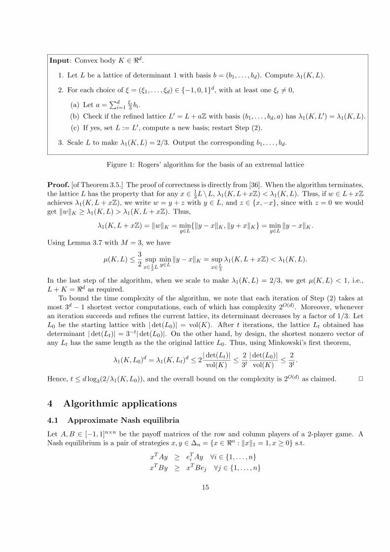
Input: Convex body K ∈ <d.

1. Let L be a lattice of determinant 1 with basis b = (b1, . . . , bd). Compute λ1(K,L).

2. For each choice of ξ = (ξ1, . . . , ξd) ∈ −1, 0, 1d, with at least one ξi 6= 0,

(a) Let a =∑d

i=1ξi3 bi.

(b) Check if the refined lattice L′ = L+ aZ with basis (b1, . . . , bd, a) has λ1(K,L′) = λ1(K,L).

(c) If yes, set L := L′, compute a new basis; restart Step (2).

3. Scale L to make λ1(K,L) = 2/3. Output the corresponding b1, . . . , bd.

Figure 1: Rogers’ algorithm for the basis of an extremal lattice

Proof. [of Theorem 3.5.] The proof of correctness is directly from [36]. When the algorithm terminates,the lattice L has the property that for any x ∈ 1

3L\L, λ1(K,L+xZ) < λ1(K,L). Thus, if w ∈ L+xZachieves λ1(K,L+ xZ), we write w = y + z with y ∈ L, and z ∈ x,−x, since with z = 0 we wouldget ‖w‖K ≥ λ1(K,L) > λ1(K,L+ xZ). Thus,

λ1(K,L+ xZ) = ‖w‖K = miny∈L‖y − x‖K , ‖y + x‖K = min

y∈L‖y − x‖K .

Using Lemma 3.7 with M = 3, we have

µ(K,L) ≤ 3

2supx∈ 1

3L

miny∈L‖y − x‖K = sup

x∈L3

λ1(K,L+ xZ) < λ1(K,L).

In the last step of the algorithm, when we scale to make λ1(K,L) = 2/3, we get µ(K,L) < 1, i.e.,L+K = <d as required.

To bound the time complexity of the algorithm, we note that each iteration of Step (2) takes atmost 3d − 1 shortest vector computations, each of which has complexity 2O(d). Moreover, wheneveran iteration succeeds and refines the current lattice, its determinant decreases by a factor of 1/3. LetL0 be the starting lattice with |det(L0)| = vol(K). After t iterations, the lattice Lt obtained hasdeterminant | det(Lt)| = 3−t|det(L0)|. On the other hand, by design, the shortest nonzero vector ofany Lt has the same length as the the original lattice L0. Thus, using Minkowski’s first theorem,

λ1(K,L0)d = λ1(K,Lt)d ≤ 2

|det(Lt)|vol(K)

≤ 2

3t| det(L0)|vol(K)

≤ 2

3t.

Hence, t ≤ d log3(2/λ1(K,L0)), and the overall bound on the complexity is 2O(d) as claimed. 2

4 Algorithmic applications

4.1 Approximate Nash equilibria

Let A,B ∈ [−1, 1]n×n be the payoff matrices of the row and column players of a 2-player game. ANash equilibrium is a pair of strategies x, y ∈ ∆n = x ∈ <n : ‖x‖1 = 1, x ≥ 0 s.t.

xTAy ≥ eTi Ay ∀i ∈ 1, . . . , nxTBy ≥ xTBej ∀j ∈ 1, . . . , n

15

Alternatively, a Nash equilibrium is a solution to the following optimization problem:

min maxiAiy + max

jxTBj − xT (A+B)y (8)

x, y ∈ ∆n. (9)

An ε-Nash equilibrium is a pair of strategies with the property that each player’s payoff cannotimprove by more than ε by moving to a different strategy, i.e.,

xTAy ≥ eTi Ay − ε ∀i ∈ 1, . . . , nxTBy ≥ xTBej − ε ∀j ∈ 1, . . . , n

Lemma 4.1 Any x, y ∈ ∆n that achieve an objective value of at most ε for (8) form an ε-Nashequilibrium.

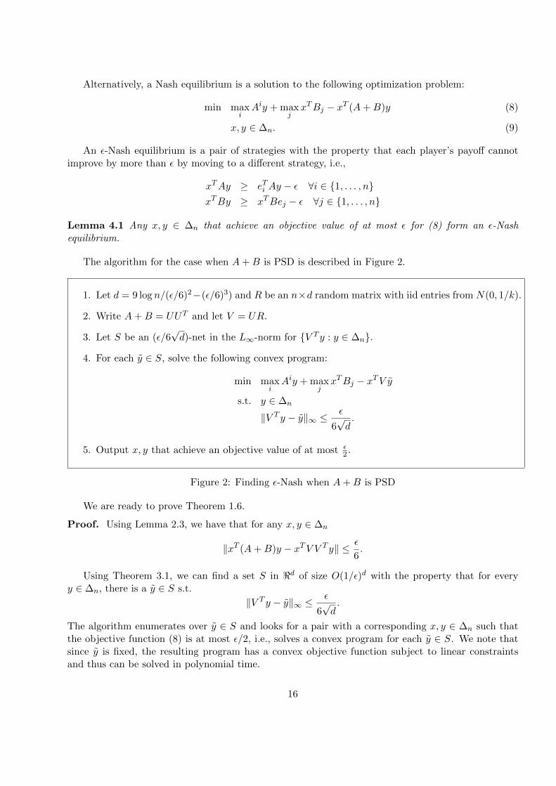
The algorithm for the case when A+B is PSD is described in Figure 2.

1. Let d = 9 log n/(ε/6)2−(ε/6)3) and R be an n×d random matrix with iid entries from N(0, 1/k).

2. Write A+B = UUT and let V = UR.

3. Let S be an (ε/6√d)-net in the L∞-norm for V T y : y ∈ ∆n.

4. For each y ∈ S, solve the following convex program:

min maxiAiy + max

jxTBj − xTV y

s.t. y ∈ ∆n

‖V T y − y‖∞ ≤ε

6√d.

5. Output x, y that achieve an objective value of at most ε2 .

Figure 2: Finding ε-Nash when A+B is PSD

We are ready to prove Theorem 1.6.

Proof. Using Lemma 2.3, we have that for any x, y ∈ ∆n

‖xT (A+B)y − xTV V T y‖ ≤ ε

6.

Using Theorem 3.1, we can find a set S in <d of size O(1/ε)d with the property that for everyy ∈ ∆n, there is a y ∈ S s.t.

‖V T y − y‖∞ ≤ε

6√d.

The algorithm enumerates over y ∈ S and looks for a pair with a corresponding x, y ∈ ∆n such thatthe objective function (8) is at most ε/2, i.e., solves a convex program for each y ∈ S. We note thatsince y is fixed, the resulting program has a convex objective function subject to linear constraintsand thus can be solved in polynomial time.

16

A solution of small objective value exists: any x, y that form a Nash equilibrium will have acorresponding y with objective value at most ε/2. Similarly any solution of objective value at mostε/2 for the program used in the algorithm implies a solution of the original quadratic program of valueat most ε, and thus satisfies the ε-Nash conditions, completing the proof. 2

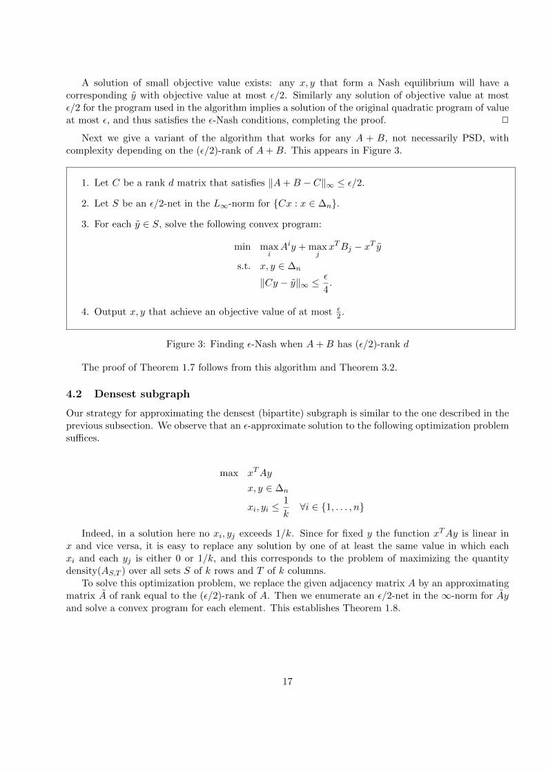
Next we give a variant of the algorithm that works for any A + B, not necessarily PSD, withcomplexity depending on the (ε/2)-rank of A+B. This appears in Figure 3.

1. Let C be a rank d matrix that satisfies ‖A+B − C‖∞ ≤ ε/2.

2. Let S be an ε/2-net in the L∞-norm for Cx : x ∈ ∆n.

3. For each y ∈ S, solve the following convex program:

min maxiAiy + max

jxTBj − xT y

s.t. x, y ∈ ∆n

‖Cy − y‖∞ ≤ε

4.

4. Output x, y that achieve an objective value of at most ε2 .

Figure 3: Finding ε-Nash when A+B has (ε/2)-rank d

The proof of Theorem 1.7 follows from this algorithm and Theorem 3.2.

4.2 Densest subgraph

Our strategy for approximating the densest (bipartite) subgraph is similar to the one described in theprevious subsection. We observe that an ε-approximate solution to the following optimization problemsuffices.

max xTAy

x, y ∈ ∆n

xi, yi ≤1

k∀i ∈ 1, . . . , n

Indeed, in a solution here no xi, yj exceeds 1/k. Since for fixed y the function xTAy is linear inx and vice versa, it is easy to replace any solution by one of at least the same value in which eachxi and each yj is either 0 or 1/k, and this corresponds to the problem of maximizing the quantitydensity(AS,T ) over all sets S of k rows and T of k columns.

To solve this optimization problem, we replace the given adjacency matrix A by an approximatingmatrix A of rank equal to the (ε/2)-rank of A. Then we enumerate an ε/2-net in the ∞-norm for Ayand solve a convex program for each element. This establishes Theorem 1.8.

17

5 Concluding remarks

We have studied the ε-rank of a real matrix A, and exhibited classes of matrices for which it islarge (Hadamard matrices, random matrices) and ones for which it is small (positive semi-definitematrices and linear combinations of those). This leads to several approximation algorithms, mainlyto problems in which the input can be approximated by a positive semi-definite matrix or a low-rank matrix. Essentially all the discussion here applies to rectangular matrices as well, and we haveconsidered square matrices just for the sake of simplicity.

It will be interesting to investigate how difficult the problem of determining or estimating theε-rank of a given real matrix is. As mentioned in the introduction, a rough approximation is given in[28].

One of our main motivating problems was the complexity of finding ε-Nash equilibria. This remainsopen for general 2-player games. Our methods do not work when the sum of the payoff matrices hashigh rank with many negative eigenvalues, e.g., for random matrices. However, in the latter case, thereis a known simple algorithm even for exact Nash equilibria, based on the existence of small supportequilibria [10]. It would be interesting to find a common generalization of this class with the classesconsidered here.

Recall that much of the earlier work regarding several notions dealing with the approximation ofmatrices by simpler ones revealed interesting applications of lower bounds, that is, of results statingthat certain matrices cannot be well approximated by very simple ones with respect to the appropriatenotions of simplicity and approximation. This is the case with the results regarding matrix rigidityand the sign-rank of matrices as well as with some of the applications in [2, 11]. It is likely to expectthat lower bounds for the ε-rank of certain matrices can yield additional interesting applications. Asa simple, not too natural and yet interesting example we mention the following.

Claim 5.1 Let p be a prime, and let X be a sample space supporting 2p random variables

X0, X1, . . . , Xp−1 and Y0, Y1, . . . , Yp−1.

Assume, further that for each i and j, the covariance Cov(Xi, Yj) satisfies |Cov(Xi, yj)−χ(i−j)| < 1/2,where the difference i− j is computed modulo p and χ(z) is the quadratic character which is 1 iff z isa quadratic residue modulo p (or 0) and −1 otherwise. Then the size of the sample space X satisfies|X| ≥ Ω(p).

This can be proved using the fact that for ε = 1/2 the ε-rank of the matrix (χ(i− j))i,j∈Zp is Ω(p),as its eigenvalues are very similar to those of a Hadamard matrix. We omit the details but note thatit will be interesting to find more natural applications of lower bounds for the ε-rank of matrices.

Finally, note that the main component in our algorithmic applications is an efficient procedure forgenerating, for a given input matrix A, a collection of not too many ε-cubes in the `∞ norm whoseunion covers the convex hull conv(A) of the columns of A. This motivates the study of Nε(A), theminimum possible size of such a collection. Thus, Nε(A) is the minimum size of a set T such that forall z ∈ conv(A) there is a t ∈ T such that ‖z− t‖∞ ≤ ε. Call a cover of conv(A) by ε-cubes an ε-net forA. The applications motivate the study of Nε(A) and that of finding efficient means of constructingε-nets for A. The focus in the present paper is to do so using the rank or approximate rank of A, andas we have mentioned one can also use the γ2 norm of A for this purpose. It turns out that there isanother complexity measure of A, its V C-dimension, that can be used here.

For a real matrix A, and a subset C of its columns, we say that A shatters C if there are realnumbers tc, c ∈ C, such that for any D ⊆ C there is a row i with A(i, c) < tc for all c ∈ D

18

and A(i, c) > tc for all c ∈ C \ D. The V C-dimension of A, denoted by V C(A) is the maximumcardinality of a shattered set of columns. We can prove that for any real m by n matrix A with entriesin [−1, 1] and V C-dimension d, Nε(A) ≤ nO(d/ε2). Moreover, an ε-net of this size can be constructeddeterministically in time proportional to its size times a polynomial factor. Note that by definition theV C-dimension of any matrix with m rows cannot exceed logm, and thus the corresponding covers arealways of size at most quasi-polynomial. We can also show that this quasi-polynomial behavior is tightin general. Therefore, while the covers obtained using this approach do not suffice to reproduce ourpolynomial time approximation algorithms obtained for matrices of logarithmic rank, they do provideimproved bounds in many cases. In particular, this approach supplies a quasi-polynomial time additiveapproximation scheme for the densest bipartite subgraph problem for any weighted graph with boundedweights. We do not include the proofs of these results here, but plan to investigate the approach aswell as some additional aspects of the γ2 approach in a subsequent work.

Acknowledgements. We are grateful to Ronald de Wolf for several helpful comments regarding therelevant work in communication complexity. We thank Daniel Dadush for bringing Rogers’ greedyconstruction paper to our attention, and for finding an error in a previous version of this paper. Veryrecently, Dadush found an algorithm to construct Rogers’ lattice using only poly(d) space with thesame 2O(d) time complexity. Thus, while his algorithm does not improve the time complexity of ourenumeration algorithm or its applications, it achieves these bounds using polynomial space.

References

[1] S. Aaronson and A. Ambainis, Quantum Search of Spatial Regions, Proc. FOCS 2003, 200-209.

[2] N. Alon, Perturbed identity matrices have high rank: proof and applications, Combinatorics,Probability and Computing 18 (2009), 3-15.

[3] N. Alon, S. Arora, R. Manokaran, D. Moshkovitz and O. Weinstein, On the inapproximability ofthe densest k-subgraph problem. Manuscript, 2011.

[4] N. Alon, S. Ben-David, N. Cesa-Bianchi and D. Haussler, Scale-sensitive dimensions, uniformconvergence, and learnability, J. ACM 44(4) (1997), 615-631.

[5] N. Alon, P. Frankl and V. Rodl, Geometrical realization of set systems and probabilistic com-munication complexity, Proc. 26th Annual Symp. on Foundations of Computer Science (FOCS),Portland, Oregon, IEEE(1985),277-280.

[6] N. Alon, W. Fernandez de la Vega, R. Kannan and M. Karpinski, Random sampling and approx-imation of MAX-CSPs. J. Comput. Syst. Sci. 67(2), 2003, 212-243. (Also in STOC 2002).

[7] N. Alon, A. Shapira and B. Sudakov, Additive approximation for Edge-deletion problems, Proc.46th IEEE FOCS, IEEE (2005), 419-428. Also: Annals of Mathematics 170 (2009), 371-411.

[8] D. Applegate and R. Kannan, Sampling and Integration of Near Log-Concave functions, STOC1991, 156-163.

[9] R. I. Arriaga, S. Vempala, An algorithmic theory of learning: Robust concepts and randomprojection. Machine Learning 63(2), 2006, 161-182 (also in FOCS 1999).

[10] I. Barany, S. Vempala and A. Vetta, Nash equilibria in random games, Random Struct. Algorithms31(4), 2007, 391-405.

19

[11] B. Barak, Z. Dvir, A. Wigderson and A. Yehudayoff, Rank bounds for design matrices withapplications to combinatorial geometry and locally correctable codes, Proc. of the 43rd annualSTOC, ACM Press (2011), 519–528.

[12] S. Ben-David, N. Eiron, and H. Simon. Limitations of learning via embeddings in Euclidean halfspaces. Journal of Machine Learning Research, 3:441–461, 2002.

[13] A. Bhaskara, M. Charikar, E. Chlamtac, U. Feige and A. Vijayaraghavan, Detecting high log-densities: an n1/4 approximation for densest - subgraph, Proc. STOC 2010, 201–210.

[14] H. Buhrman, N. Vereshchagin, and R. de Wolf. On computation and communication with smallbias. In Proceedings of the 22nd IEEE Conference on Computational Complexity, pages 24–32.IEEE, 2007.

[15] H. Buhrman, R. de Wolf. Communication Complexity Lower Bounds by Polynomials, Proc. ofthe 16th IEEE Annual Conference on Computational Complexity, 2001, 120–130.

[16] D. Dadush, C. Peikert and S. Vempala, Enumerative Lattice Algorithms in any Norm Via M-ellipsoid Coverings. Proc. FOCS 2011, 580-589.

[17] D. Dadush and S. Vempala, Near-optimal deterministic algorithms for volume computation viaM-ellipsoids. Proc. of the National Academy of Sciences, September 2013.

[18] W. Fernandez de la Vega, M. Karpinski, R. Kannan and S. Vempala: Tensor decomposition andapproximation schemes for constraint satisfaction problems, Proc. of STOC 2005, 747-754.

[19] A. Frieze and R. Kanan, Quick approximation to matrices and applications, Combinatorica, 19(1999), pp. 175–220.

[20] J. Forster, A linear lower bound on the unbounded error probabilistic communication complexity,in SCT: Annual Conference on Structure in Complexity Theory, 2001. Also: JCSS, 65 (2002),612–625.

[21] J. Forster, N. Schmitt, and H. U. Simon. Estimating the optimal margins of embeddings ineuclidean half spaces. Technical Report NC2-TR-2001-094, NeuroCOLT2 Technical Report Series,2000.

[22] Joel N. Franklin, Matrix Theory, Dover Publications, 1993.

[23] M. Grotschel, L. Lovasz and A. Schrijver, Geometric Algorithms and Combinatorial Optimization.Springer, 1988.

[24] V. Guruswami, D. Micciancio and O. Regev, The complexity of the covering radius problem.Computational Complexity, 14(2), pp. 90-121, 2005.

[25] W. B. Johnson and J. Lindenstrauss, Extensions of Lipschitz maps into a Hilbert space, ContempMath 26, 1984, 189–206.

[26] R. Kannan and T, Theobald. Games of fixed rank: A hierarchy of bimatrix games, Econom.Theory 42:157-173, 2010 (also in SODA 2007).

[27] M. Krause, Geometric arguments yield better bounds for threshold circuits and distributed com-puting, Theoretical Computer Science, 156 (1996), 99–117.

20

[28] T. Lee, A. Shraibman. An approximation algorithm for approximation rank, Proc. of the 24thIEEE Conference on Computational Complexity, 2009, 351–357.

[29] N. Linial, S. Mendelson, G. Schechtman, and A. Shraibman. Complexity measures of sign matri-ces. Combinatorica, 27 (2007), 439–463.

[30] N. Linial and A. Shraibman. Lower bounds in communication complexity based on factorizationnorms. Random Structures and Algorithms, 34:368–394, 2009.

[31] R. J. Lipton, E. Markakis, A. Mehta: Playing large games using simple strategies. ACM Confer-ence on Electronic Commerce 2003: 36-41.

[32] R. Mathias. The Hadamard operator norm of a circulant and applications. SIAM journal onmatrix analysis and applications, 14(4):1152–1167, 1993.

[33] G. Pisier, The Volume of Convex Bodies and Banach Space Geometry, Second Ed., CambridgeUniversity Press, 1999.

[34] A. A. Razborov, Quantum communication complexity of symmetric predicates, arXiv:quant-ph/0204025, 2002.

[35] A. A. Razborov and A. A. Sherstov, The Sign-Rank of AC0, SIAM J. Comput. 39(5), 1833-1855(2010).

[36] C. A. Rogers, A note on coverings and packings. J. London Math. Soc. 25, (1950). 327–331.

[37] C. A. Rogers, Lattice coverings of space with convex bodies. J. London Math. Soc. 33, 1958,208–212.

[38] C. A. Rogers, Lattice covering of space: The Minkowski-Hlawka theorem. Proc. London Math.Soc. (3) 8, 1958, 447–465.

[39] C. A. Rogers, Lattice coverings of space. Mathematika 6, 1959, 33–39.

[40] A. Sherstov. Halfspace matrices. Computational Complexity, 17(2):149–178, 2008.

[41] J. H. Spencer, Six standard deviations suffice, Trans. Amer. Math. Soc. 289 (1985), 679–706.

[42] L. G. Valiant, Graph-theoretic arguments in low-level complexity, Lecture notes in ComputerScience 53 (1977), Springer, 162-176.

[43] S. Vempala, The Random Projection Method, AMS, 2004.

[44] H. E. Warren, Lower Bounds for approximation by nonlinear manifolds, Trans. Amer. Math. Soc.133 (1968), 167-178.

21