Embed Size (px)
Citation preview
The Approach of Moments for PolynomialEquations
Monique Laurent1 and Philipp Rostalski2
1 Centrum voor Wiskunde en Informatica, Science Park 123, 1098 XGAmsterdam, and Tilburg University, P.O. Box 90153, 5000 LE Tilburg,Netherlands. [email protected]
2 Department of Mathematics, UC Berkeley, 1067 Evans Hall, Berkeley, CA94720-3840, USA. [email protected]
Summary. In this chapter we present the moment based approach for computingall real solutions of a given system of polynomial equations. This approach buildsupon a lifting method for constructing semidefinite relaxations of several nonconvexoptimization problems, using sums of squares of polynomials and the dual theory ofmoments. A crucial ingredient is a semidefinite characterization of the real radicalideal, consisting of all polynomials with the same real zero set as the system of poly-nomials to be solved. Combining this characterization with ideas from commutativealgebra, (numerical) linear algebra and semidefinite optimization yields a new classof real algebraic algorithms. This chapter sheds some light on the underlying theoryand the link to polynomial optimization.
1 Introduction
Computing all points x ∈ Kn (K = R or C) at which a given system ofpolynomials in n variables
h1, . . . , hm ∈ R[x1, . . . , xn] = R[x]
vanishes simultaneously, is an old problem arising in many mathematical mod-els in science and engineering, with numerous applications in different areasranging from control, cryptography, computational geometry, coding theoryand computational biology to optimization, robotics, statistics and many oth-ers (see, e.g., [44]). In this chapter we will focus on the characterization andthe (numerical) computation of all real roots or, more generally, of all rootslying in some given basic semi-algebraic set, i.e. satisfying some prescribedpolynomial inequalities. A variety of methods has been proposed to tacklesuch problems, some of which will be briefly recalled in the next section. Inthis chapter we will focus on a new approach based on sums of squares ofpolynomials and the dual theory of moments. In this context, semidefinite
2 Monique Laurent and Philipp Rostalski
programming will be the tool permitting to distinguish algorithmically be-tween real and complex nonreal elements.
1.1 Existing methods
Solving polynomial equations has a long tradition covered in a vast literature;for information and further references see e.g. the monographs of Basu, Pollackand Roy [2], Dickenstein and Emiris [9], Mora [27, 28], Elkadi and Mourrain[10], Stetter [43], Sturmfels [44]. We do not attempt a complete description ofall existing methods, but instead we only try to give a coarse classification.Most existing algorithms can be roughly categorized according to the followingcriteria: local vs. global search, numerical vs. exact/symbolic computation,and solving over the complex numbers vs. solving over the real numbers.
Over the complex numbers
Symbolic methods. Grobner bases, resultants or, more generally, borderbases and generalized normal form algorithms are typical representatives ofthis class of methods. The main idea is to compute the structure of the quo-tient algebra R[x]/I (where I is the ideal generated by the given polynomialshi) and to use this information to characterize the roots, e.g., using the shapelemma, or Stickelberger’s theorem (viz. the eigenvalue method), or the ratio-nal univariate representation.
The following basic fact plays a crucial role: The system of polynomialequations h1 = · · · = hm = 0 has finitely many roots if and only if thequotient ring R[x]/I of the underlying ideal I = 〈h1, . . . , hm〉 is finite dimen-sional as a vector space. This in turn enables to reduce the computation ofall complex roots to tasks of finite dimensional linear algebra (like eigenvaluecomputations). Roughly speaking, the basic idea is to replace the given systemhi = 0 by a new equivalent system gj = 0 with the same set of complex roots,but with a much easier structure facilitating the extraction of the roots.
For instance, one may find an equivalent system comprising polynomialsin triangular form g1 ∈ R[x1], g2 ∈ R[x1, x2], . . . , gn ∈ R[x1, . . . , xn], whichcan be solved by solving a sequence of univariate root finding problems. Suchan approach suffers however from the propagation of numerical errors andtriangular representations are difficult to compute, typically involving lexico-graphic Grobner bases. A more efficient approach is the rational univariaterepresentation, where the new system has a parametric representation:
x1 = h1(t)/h(t), . . . , xn = hn(t)/h(t), f(t) = 0 (hi, h, f ∈ R[t]),
which requires the solution of a single univariate polynomial: f(t) = 0 (see[38]).
Symbolic-numeric methods. Motivated by the great success of numeri-cal linear algebra, a new trend in applied mathematics is to carefully combine

The Approach of Moments for Polynomial Equations 3
symbolic methods (mostly border bases methods) with numerical calculations,such as singular value decomposition, LU-factorization and other workhorsesof numerical linear algebra in order to derive powerful algorithms for largescale problems (see e.g. [30] for details). As mentioned above, symbolic meth-ods are able to transform the given system hi = 0 into a new, better struc-tured system gj = 0. Then the task of computing the complex roots is reducedto (numerical) linear algebra, like computing the eigenvalues/eigenvectors ofcompanion matrices (cf. Section 2.2 below), or univariate root finding.
Numerical methods. The most successful approach in this class of methodsis homotopy continuation. Such methods rely on Bertini’s theorem allowing todeform an easier instance with known solutions of the class of problems to besolved into the original system, without encountering singularities along thepath (cf. [40] for details). Keeping track of the roots during this deformationallows to compute the desired roots.
Over the real numbers
While the task of solving polynomial equations over the complex numbersis relatively well understood, computing only the real roots is still largelyopen. The need for methods tailored to real root finding is mainly motivatedby applications, where often only the real roots are meaningful, and whosenumber is typically much smaller than the total number of complex solutions.As an illustration, just consider the simple equation x21 + x22 = 0, where noteven the dimensions of the real and complex solution sets agree!
So far, real solving methods were mostly build upon local methods com-bined with a bisection search strategy. More recently, two new global ap-proaches have been considered which can be seen as refinements of complexroot finding methods mentioned above: the SDP based moment approach(which is the focus of this chapter), and a new homotopy continuation methodtuned to real roots. The three main classes of methods for real roots are:
Subdivision methods. Combining exclusion criteria to remove parts of thesearch space not containing any real root and identify regions containing iso-lated real roots, with local search strategies such as Newton-Raphson or higherorder methods are the basis for the class of subdivision methods. The searchspace is subdivided until it contains only a single root and Newton’s methodconverges (cf. e.g. [31] for a recent account). Exclusion criteria include real rootcounting techniques based e.g. on Sturm-Habicht sequences, Descartes’ ruleof signs (for univariate polynomials), or signatures of Hermite forms (in themultivariate case). Such techniques, combined with deformation techniquesusing Puiseux series, are also extended to the problem of computing at leastone point in each connected component of an algebraic variety (possibly ofpositive dimension) (cf. [2] for a detailed account).
Khovanskii-Rolle continuation. This method is a recent extension of curvefollowing methods (like homotopy continuation for complex roots) tailored to
4 Monique Laurent and Philipp Rostalski
real roots. It exploits the fact that there are sharp bounds for the number ofreal roots of systems of equations with few monomials, combined with Galeduality. The approach allows to track significantly fewer paths of an auxiliarysystem leading to all nondegenerate real solutions of the original system. It isstill under investigation, but has the potential to become an efficient algorithmfor real root finding (see [3, 41] for details).
Moment methods. This class of methods was first proposed in [17] withextensions in [18, 19], and is the focus of this chapter. The basic idea isto compute the real roots by working in a smaller quotient space, obtainedby taking the quotient by the real radical ideal R
√I of the original ideal I,
consisting of all polynomials that vanish at the set of common real roots ofthe original system hi = 0. In this way, computing the real roots is againreduced to a task of numerical linear algebra, now in the finite dimensionalvector space R[x]/ R
√I (assuming only that the number of real roots is finite,
while the total number of complex roots could be infinite). Finding the realradical ideal is achieved by computing the kernel of a generic moment matrixobtained by solving iteratively certain semidefinite programming problems.
1.2 The basic idea of the moment method
Most symbolic and symbolic/numeric algorithms for solving a system of poly-nomials decompose the structure of the polynomial ring into its ideal structure(namely, the ideal I generated by the equations to be solved) and its vectorspace structure (corresponding to the quotient of the polynomial ring by thisideal). While the former is treated with symbolic methods one can use efficientlinear algebra for the latter. We start with an elementary introduction. Let
h1(x) = · · · = hm(x) = 0 (1)
be the system of polynomial equations to be solved. Denote by D ∈ N themaximum degree of the polynomials hi and let I = 〈h1, . . . , hm〉 be the idealgenerated by these polynomials, i.e., the set of all polynomials
∑i uihi with
ui ∈ R[x]. If we form the matrix H whose rows are the coefficient vectors ofthe polynomials hi, then the roots of the system (1) are precisely the elementsx ∈ Cn satisfying H[x]D = 0, where for any integer t ∈ N,
[x]t = (1, x1, . . . , xn, x21, x1x2, . . . , x
tn)
denotes the vector of all monomials of degree at most t. Augmenting the sys-tem (1) with new polynomials obtained by multiplying the hi’s by monomialsdoes not change its set of common roots. Given an integer t, we add all possi-ble multiples of the hi’s with degree at most t, i.e., we add all ‘valid’ equations:xαhi = 0 where |α| ≤ t − deg(hi). This yields a new, larger system of poly-nomials whose coefficient vectors make the rows of a matrix Ht (known asSylvester or Macaulay-like matrix). Again, the roots of (1) are those elementsx ∈ Cn satisfying Ht[x]t = 0.
The Approach of Moments for Polynomial Equations 5
The basic idea is to linearize this system of equations by introducing vari-ables y = (yα) for the monomials xα and to solve instead a linear system:
Hty = 0. (2)
The kernel of the matrix Ht is a linear subspace, which contains the vectors[x]t for all roots x of the system (1) and thus also their linear span. Whenthe system (1) has finitely many complex roots, it turns out that, for t largeenough, (some projection of) the kernel of Ht coincides with the linear span ofthe monomial vectors corresponding to the roots of (1), which opens the wayto extracting the roots. More precisely, the central observation (dating back to[23]) is that for t large enough a Gaussian elimination on the Sylvester matrixHt will reveal a Grobner basis for the ideal I and thus the desired quotientring structure R[x]/I. This in turn can be used to reduce the multivariate rootfinding problem to a simple eigenvalue calculation (as recalled in Section 2.2).
If we want to compute the real roots only, we need a mechanism to cancelout all (or as many as possible) nonreal solutions among the complex ones.This cancellation can be done by augmenting the original system (1) withadditional polynomials derived from sums of squares of polynomials in theideal I. We introduce this idea by means of a simple example.
Example 1. Consider the ideal I ⊆ R[x1, x2] generated by the polynomialh = x21 + x22. The complex variety is positive dimensional, since it consists ofinfinitely many complex roots: x2 = ±ix1 (x1 ∈ C), while the origin (0, 0) isthe only real root. If we add the two polynomials p1 = x1, p2 = x2 to I the realvariety remains unchanged, but none of the complex nonreal roots survives thisintersection. Note that p1, p2 have the property that the polynomial p21+p22 = his a sum of squares of polynomials belonging to I.
This example illustrates the following fact: If the pi’s are polynomials forwhich
∑i p
2i ∈ I, then each pi vanishes at all the real roots of the ideal I (but
not necessarily at its complex nonreal roots!). Thus we can add the pi’s tothe original system (1) without altering its set of real roots. The formal toolbehind this augmentation is the Real Nullstellensatz (see Theorem 1), whichstates that the set of real solutions to the system (1) remains unchanged if weadd to it any polynomial appearing with an even degree in a sum of squarespolynomial that belongs to I. The set of all such polynomials is known asthe real radical ideal of I, denoted as R
√I (see Section 2 for definitions). A
main feature of the moment matrix method is that it permits to generate thepolynomials in the real radical ideal in a systematic way, using duality.
Let us first look directly at the additional properties that are satisfiedby a vector y = [x]t ∈ Ker Ht, when x is a real root of (1). Obviously thematrix [x]s[x]Ts is positive semidefinite for any integer s and by ‘linearizing’(replacing xα by yα) we obtain the following matrix of generalized Hankeltype: Ms(y) = (yα+β)α,β∈Nn
s. Matrices with this generalized Hankel structure
6 Monique Laurent and Philipp Rostalski
are also known as moment matrices (see Definition 3). As an illustration wedisplay Ms(y) for the case n = 2:
[x]s[x]Ts =
1 x1 x2 x21 . . .x1 x21 x1x2 x31 . . .x2 x1x2 x22 x21x2 . . .x21 x31 x21x2 x41 . . ....
......
.... . .
Ms(y)
1 y10 y01 y20 . . .y10 y20 y11 y30 . . .y01 y11 y02 y21 . . .y20 y30 y21 y40 . . ....
......
.... . .
.
Therefore, we can restrict the search in the kernel of the Sylvester matrix Ht
to the vectors y satisfying the additional positive semidefiniteness condition:Ms(y) � 0 for all s ≤ t/2. This condition captures precisely the ‘real algebraic’nature of real numbers vs. complex numbers, as it would not be valid forvectors y corresponding to complex nonreal roots.
Example 2. (Example 1 cont.) Say we wish to compute the real roots of thepolynomial h = x21 + x22. After linearization, the constraint Hy = 0 reads:y20 + y02 = 0. Positive semidefiniteness requires y20 ≥ 0, y02 ≥ 0 which,combined with y20 + y02 = 0 implies y20 = y02 = 0 and thus y10 = y01 =y11 = 0 (using again M1(y) � 0). Therefore, we find y = (1, 0, 0, 0, 0, 0) as theunique solution, so that y = [x]2 corresponds to the unique real root x = (0, 0)of h. The kernel of M1(y) contains the vectors (0, 1, 0) and (0, 0, 1), which canbe seen as the coefficient vectors of the two polynomials p1 = x1 and p2 = x2in the monomial basis {1, x1, x2} of R[x]1. In other words the kernel of M1(y)already contains a basis of the real radical ideal R
√I.
Although the above example is extremely simplistic, it conveys the main idea:The kernel of Ms(y) characterizes (for s large enough) the real radical idealand plays the role of the range space of H in standard normal form algorithms.
1.3 Organization of the chapter
First we recall some basic material from polynomial algebra in Section 2. Thismaterial can be found in most standard textbooks and is used throughout thechapter. The relation between moment matrices and real radical ideals as wellas the moment method for real root finding is discussed in Section 3. Thissection and in particular the semidefinite characterization of the real radicalideal form the heart of the chapter. We also discuss the link to some complexroot finding methods and in Section 4 we briefly touch some related topics:polynomial optimization and the study of semi-algebraic sets, emptyness cer-tificates, positive dimensional varieties, and quotient ideals. Throughout thechapter we illustrate the results with various examples.
The Approach of Moments for Polynomial Equations 7
2 Preliminaries of polynomial algebra
2.1 Polynomial ideals and varieties
The polynomial ring and its dual. For the sake of simplicity we deal withpolynomials with real coefficients only although some results remain validfor polynomials with complex coefficients. Throughout R[x] := R[x1, . . . , xn]denotes the ring of multivariate polynomials in n variables. For α ∈ Nn, xα
denotes the monomial xα11 · · ·xαn
n , with degree |α| :=∑ni=1 αi. Set Nnt :=
{α ∈ Nn | |α| ≤ t} and let
[x]∞ = (xα)α∈Nn , [x]t = (xα)α∈Nnt
denote the vectors comprising all monomials (resp., all monomials of de-gree at most t) in n variables. A polynomial p ∈ R[x] can be written asp =
∑α∈Nn pαx
α with finitely many nonzero pα’s; its support is the set ofmonomials appearing with a nonzero coefficient, its (total) degree deg(p) isthe largest degree of a monomial in the support of p, and vec(p) = (pα) de-notes the vector of coefficients of p. The set R[x]t consists of all polynomialswith degree at most t.
Given a vector space A on R, its dual space A∗ consists of all linear func-tionals from A to R. The orthogonal complement of a subset B ⊆ A is
B⊥ := {L ∈ A∗ | L(b) = 0 ∀b ∈ B}
and SpanR(B) denotes the linear span of B. Then, SpanR(B) ⊆ (B⊥)⊥, withequality when A is finite dimensional. We consider here the case A = R[x]and A = R[x]t. Examples of linear functionals on R[x] are the evaluation
Λv : p ∈ R[x] 7→ Λv(p) = p(v) (3)
at a point v ∈ Rn and, more generally, the differential functional
∂αv : p ∈ R[x] 7→ ∂αv (p) =1∏n
i=1 αi!
(∂|α|
∂xα11 . . . ∂xαn
np
)(v), (4)
which evaluates at v ∈ Rn the (scaled) α-th derivative of p (where α ∈ N).For α = 0, ∂αv coincides with the evaluation at v, i.e., ∂0v = Λv. For α, β ∈ Nn,
∂α0 (xβ) = 1 if α = β, and 0 otherwise.
Therefore, any linear form Λ ∈ R[x]∗ can be written in the form:
Λ =∑α∈Nn
Λ(xα)∂α0 .
This is in fact a formal power series as in general infinitely many Λ(xα) arenonzero. Let y = (yα) denote the coefficient series of Λ in (∂α0 ) i.e. yα = Λ(xα),
8 Monique Laurent and Philipp Rostalski
such that Λ(p) = yT vec(p) for all p ∈ R[x]. For instance, the evaluation atv ∈ Rn reads Λv =
∑α v
α∂α0 , with coefficient series [v]∞ = (vα)α∈Nn in (∂α0 ).
Ideals and varieties. A linear subspace I ⊆ R[x] is an ideal if p ∈ I, q ∈ R[x]implies pq ∈ I. The ideal generated by h1, . . . , hm ∈ R[x] is defined as
I = 〈h1, . . . hm〉 :={ m∑j=1
ujhj | u1, . . . , um ∈ R[x]}
and the set {h1, . . . , hm} is then called a basis of I. By the finite basis theo-rem [6, §2.5, Thm. 4], every ideal in R[x] admits a finite basis. Given an idealI ⊆ R[x], the algebraic variety of I is the set
VC(I) = {v ∈ Cn | hj(v) = 0 ∀j = 1, . . . ,m}
of common complex zeros to all polynomials in I and its real variety is
VR(I) := VC(I) ∩ Rn.
The ideal I is said to be zero-dimensional when its complex variety VC(I) isfinite. The vanishing ideal of a subset V ⊆ Cn is the ideal
I(V ) := {f ∈ R[x] | f(v) = 0 ∀v ∈ V } .
For an ideal I ⊆ R[x], we may also define the ideal
√I :=
{f ∈ R[x]
∣∣ fm ∈ I for some m ∈ N \ {0}},
called the radical ideal of I, and the real radical ideal (or real ideal)
R√I :=
{p ∈ R[x]
∣∣ p2m +∑j
q2j ∈ I for some qj ∈ R[x],m ∈ N \ {0}}.
An ideal I is said to be radical (resp., real radical) if I =√I (resp., I = R
√I).
For instance, the ideal I = 〈x21 + x22〉 is not real radical since x1, x2 ∈ R√I \ I.
As can be easily verified, I is radical if and only if p2 ∈ I implies p ∈ I, andI is real radical if and only if
∑i p
2i ∈ I implies pi ∈ I for all i. We have the
following chains of inclusion:
I ⊆√I ⊆ I(VC(I)), I ⊆ R
√I ⊆ I(VR(I)).
The relation between vanishing and (real) radical ideals is stated in the fol-lowing two famous theorems:
Theorem 1. Let I ⊆ R[x] be an ideal.
(i) Hilbert’s Nullstellensatz (see, e.g., [6, §4.1]) The radical ideal of I isequal to the vanishing ideal of its variety, i.e.,
√I = I(VC(I)).
(ii) Real Nullstellensatz (see, e.g., [4, §4.1]) The real radical ideal of I isequal to the vanishing ideal of its real variety, i.e., R
√I = I(VR(I)).
The Approach of Moments for Polynomial Equations 9
2.2 The eigenvalue method for complex roots
The quotient space R[x]/I. The quotient set R[x]/I consists of all cosets[f ] := f + I = {f + q | q ∈ I} for f ∈ R[x], i.e. all equivalent classes ofpolynomials in R[x] modulo I. This quotient set R[x]/I is an algebra with ad-dition [f ] + [g] := [f + g], scalar multiplication λ[f ] := [λf ] and multiplication[f ][g] := [fg], for λ ∈ R, f, g ∈ R[x]. The following classical result relates thedimension of R[x]/I and the cardinality of the variety VC(I) (see e.g. [6, 43]).
Theorem 2. Let I be an ideal in R[x]. Then,
|VC(I)| <∞⇐⇒ dimR[x]/I <∞.
Moreover, |VC(I)| ≤ dim R[x]/I, with equality if and only if I is radical.
Assume that the number of complex roots is finite and set N := dimR[x]/I, sothat |VC(I)| ≤ N <∞. Consider a set B := {b1, . . . , bN} ⊆ R[x] for which thecosets [b1], . . . , [bN ] are pairwise distinct and {[b1], . . . , [bN ]} is a (linear) basisof R[x]/I. By abuse of language we also say that B itself is a basis of R[x]/I.
Then every f ∈ R[x] can be written in a unique way as f =∑Ni=1 cibi + p,
where ci ∈ R and p ∈ I. The polynomial
NB(f) :=
N∑i=1
cibi
is called the normal form of f modulo I with respect to the basis B. In otherwords, we have the direct sum decomposition:
R[x] = SpanR(B)⊕ I,
and SpanR(B) and R[x]/I are isomorphic vector spaces. We now introduce theeigenvalue method for computing all roots of a zero-dimensional ideal, whichwe first describe in the univariate case.
Computing roots with companion matrices. Consider first a univariatepolynomial p = xd − ad−1xd−1 − . . . − a1x − a0 and the ideal I = 〈p〉. Thenthe set B = {1, x, . . . , xd−1} is a basis of R[x]/I. The following matrix
X :=
(0 a0
Id−1 a
)where a = (a1, . . . , ad−1)T ,
is known as the companion matrix of the polynomial p. One can easily verifythat det(X − xI) = (−1)dp(x), so that the eigenvalues of X are precisely theroots of the polynomials p. Therefore the roots of a univariate polynomialcan be found with an eigenvalue computation. Moreover, the columns of thecompanion matrix X correspond to the normal forms of the monomials inxB = {x, x2, . . . , xd} modulo I with respect to the basis B. As we now seethese facts extend naturally to the multivariate case.
10 Monique Laurent and Philipp Rostalski
Given h ∈ R[x], we define the multiplication (by h) operator in R[x]/I as
Xh : R[x]/I −→ R[x]/I[f ] 7−→ Xh([f ]) := [hf ] ,
(5)
which can be represented by its matrix (again denoted Xh for simplicity) with
respect to the basis B of R[x]/I. Namely, if we set NB(hbj) :=∑Ni=1 aijbi
(where aij ∈ R), then the jth column of Xh is the vector (aij)Ni=1. Note also
that, since hbj −NB(hbj) ∈ I, polynomials in I can be read directly from Xh.This fact will play an important role for border bases (see Section 2.3). Inthe univariate case, when I = 〈p〉 and h = x, the multiplication matrix Xxis precisely the companion matrix X of p introduced above. Throughout wealso denote by Xi := Xxi
the multiplication operator by the variable xi in themultivariate case.
The following famous result (see e.g. [5, Chap. 2§4]) relates the eigenvaluesof the multiplication operators in R[x]/I to the algebraic variety VC(I). Thisresult underlies the well known eigenvalue method, which plays a central rolein many algorithms for complex root solving.
Theorem 3. (Stickelberger theorem) Let I be a zero-dimensional idealin R[x], let B be a basis of R[x]/I, and let h ∈ R[x]. The eigenvalues of themultiplication operator Xh are the evaluations h(v) of the polynomial h at thepoints v ∈ VC(I). Moreover, for all v ∈ VC(I),
(Xh)T [v]B = h(v)[v]B,
setting [v]B = (b(v))b∈B; that is, the vector [v]B is a left eigenvector of themultiplication operator with eigenvalue h(v).
Therefore the eigenvalues of the matrices Xi are the ith coordinates of thepoints v ∈ VC(I), which can be derived from the left eigenvectors [v]B. Practi-cally, one can recover the roots from the left eigenvectors when the eigenspacesof X Th all have dimension one. This is the case when the values h(v) (v ∈ VC(I))are pairwise distinct (easy to achieve, e.g., if we choose h to be a generic lin-ear form) and when the ideal I is radical (since the dimension of R[x]/I isthen equal to the number of roots so that the vectors [v]B (v ∈ VC(I)) form acomplete basis of eigenvectors).
Summarizing, the task of solving a system of polynomial equations is re-duced to a task of numerical linear algebra once a basis of R[x]/I and a normalform algorithm are available, as they permit the construction of the multipli-cation matrices Xi, Xh. Moreover, the roots v ∈ VC(I) can be successfullyconstructed from the eigenvectors/eigenvalues of Xh when I is radical andh is generic. Our strategy for computing the real variety VR(I) will be tocompute a linear basis of the quotient space R[x]/ R
√I and the correspond-
ing multiplication matrices, so that we we can apply the eigenvalue methodprecisely in this setting of having a radical (even real radical) ideal.
The Approach of Moments for Polynomial Equations 11
The number of (real) roots can be counted using Hermite’s quadratic form:
Sh : R[x]/I × R[x]/I → R([f ], [g]) 7→ Tr(Xfgh).
Here, Tr(Xfgh) is the trace of the multiplication (by the polynomial fgh)matrix. As Sh is a symmetric matrix, all its eigenvalues are real. Denote byσ+(Sh) (resp., σ−(Sh)) its number of positive (resp., negative) eigenvalues.The following classical result shows how to count the number of roots satis-fying prescribed sign conditions (cf. e.g. [2]).
Theorem 4. Let I ⊆ R[x] be a zero-dimensional ideal and h ∈ R[x]. Then,
rankSh = |{v ∈ VC(I) | h(v) 6= 0}| ,
σ+(Sh)− σ−(Sh) = |{v ∈ VR(I) | h(v) > 0}| − |{v ∈ VR(I) | h(v) < 0}| .In particular, for the constant polynomial h = 1,
rank(S1) = |VC(I)| and σ+(S1)− σ−(S1) = |VR(I)|.
2.3 Border bases and normal forms
The eigenvalue method for solving polynomial equations (described in the pre-ceding section) requires the knowledge of a basis of R[x]/I and of an algorithmto compute the normal form of a polynomial with respect to this basis.
A well known basis of R[x]/I is the set of standard monomials with respectto some monomial ordering. The classical way to find standard monomials isto construct a Grobner basis of I (then the standard monomials are the mono-mials not divisible by any leading monomial of a polynomial in the Grobnerbasis). Moreover, once a Grobner basis is known, the normal form of a poly-nomial can be found via a polynomial division algorithm (see, e.g., [6, Chap.1] for details). Other techniques have been proposed, producing more gen-eral bases which do not depend on a specific monomial ordering and oftenare numerically more stable. In particular, algorithms have been proposedfor constructing border bases of I leading to general (connected to 1) basesof R[x]/I (see [9, Chap. 4], [14], [29], [43]); these objects are introduced be-low. The moment matrix approach for computing real roots presented in thischapter leads naturally to the computation of such general bases.
Definition 1. Given a set B of monomials, define the new sets of monomials
B+ := B ∪n⋃i=1
xiB = B ∪ {xib | b ∈ B, i = 1, . . . , n} , ∂B = B+ \ B,
called, respectively, the one-degree prolongation of B and the border of B. Theset B is said to be connected to 1 if 1 ∈ B and each m ∈ B\{1} can be writtenas m = xi1 . . . xik with xi1 , xi1xi2 , . . . , xi1 · · ·xik ∈ B. Moreover, B is said tobe stable by division if all divisors of m ∈ B also belong to B. Obviously, B isconnected to 1 if it is stable by division.
12 Monique Laurent and Philipp Rostalski
Assume B is a set of monomials which is connected to 1. For each bordermonomial m ∈ ∂B, consider a polynomial fm of the form
fm := m− rm, where rm ∈ SpanR(B). (6)
The family F := {fm | m ∈ ∂B} is called a rewriting family for B in [30, 32].Using F , one can express all border monomials in ∂B as linear combinationsof monomials in B modulo the ideal 〈F 〉. Moreover, the rewriting family Fcan be used in a division algorithm to rewrite any polynomial p ∈ R[x] as
p = r +∑m∈∂B
umfm, where r ∈ SpanR(B), um ∈ R[x]. (7)
This expression is in general not unique, as it depends on the order in whichthe polynomials of F are used throughout the division process.
Example 3. Let B = {1, x1, x2} with border set ∂B = {x21, x1x2, x22}, andconsider the rewriting family
F = {fx21
= x21 + 1, fx1x2= x1x2 − 1, fx2
2= x22 + 1}.
There are two possibilities to rewrite the polynomial p = x21x2. Either, firstdivide by fx1x2 and obtain p = x21x2 = x1fx1x2 + x1 with r = x1, or firstdivide by fx2
1and obtain p = x21x2 = x2fx2
1− x2 with r = −x2.
In view of (7), the set B spans the vector space R[x]/〈F 〉, but is in generalnot linearly independent. Linear independence guaranties uniqueness of thedecomposition (7) and, as Theorem 5 below shows, is equivalent to the com-mutativity of certain formal multiplication operators.
Consider the linear operator Xi : SpanR(B)→ SpanR(B) defined using therewriting family F , namely, for b ∈ B,
Xi(b) =
{xib if xib ∈ B,xib− fxib = rxib otherwise,
and extend Xi to SpanR(B) by linearity. Denote also by Xi the matrix of thislinear operator, which can be seen as a formal multiplication (by xi) matrix.
Theorem 5. [29] Let F be a rewriting family for a set B of monomials con-nected to 1, and consider the ideal J := 〈F 〉. The following conditions areequivalent:
(i) The formal multiplication matrices X1, . . . ,Xn commute pairwise.(ii) The set B is a (linear) basis of R[x]/J , i.e., R[x] = SpanR(B)⊕ J .
Then, the set F is said to be a border basis of the ideal J , and the matrix Xirepresents the multiplication operator by xi in R[x]/J with respect to B.
The Approach of Moments for Polynomial Equations 13
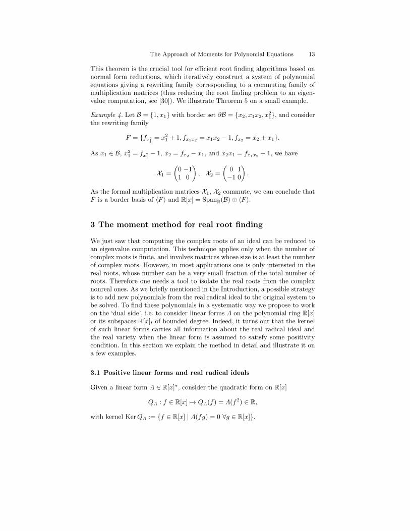
This theorem is the crucial tool for efficient root finding algorithms based onnormal form reductions, which iteratively construct a system of polynomialequations giving a rewriting family corresponding to a commuting family ofmultiplication matrices (thus reducing the root finding problem to an eigen-value computation, see [30]). We illustrate Theorem 5 on a small example.
Example 4. Let B = {1, x1} with border set ∂B = {x2, x1x2, x21}, and considerthe rewriting family
F = {fx21
= x21 + 1, fx1x2= x1x2 − 1, fx2
= x2 + x1}.
As x1 ∈ B, x21 = fx21− 1, x2 = fx2
− x1, and x2x1 = fx1x2+ 1, we have
X1 =
(0 −11 0
), X2 =
(0 1−1 0
).
As the formal multiplication matrices X1, X2 commute, we can conclude thatF is a border basis of 〈F 〉 and R[x] = SpanR(B)⊕ 〈F 〉.
3 The moment method for real root finding
We just saw that computing the complex roots of an ideal can be reduced toan eigenvalue computation. This technique applies only when the number ofcomplex roots is finite, and involves matrices whose size is at least the numberof complex roots. However, in most applications one is only interested in thereal roots, whose number can be a very small fraction of the total number ofroots. Therefore one needs a tool to isolate the real roots from the complexnonreal ones. As we briefly mentioned in the Introduction, a possible strategyis to add new polynomials from the real radical ideal to the original system tobe solved. To find these polynomials in a systematic way we propose to workon the ‘dual side’, i.e. to consider linear forms Λ on the polynomial ring R[x]or its subspaces R[x]t of bounded degree. Indeed, it turns out that the kernelof such linear forms carries all information about the real radical ideal andthe real variety when the linear form is assumed to satisfy some positivitycondition. In this section we explain the method in detail and illustrate it ona few examples.
3.1 Positive linear forms and real radical ideals
Given a linear form Λ ∈ R[x]∗, consider the quadratic form on R[x]
QΛ : f ∈ R[x] 7→ QΛ(f) = Λ(f2) ∈ R,
with kernel KerQΛ := {f ∈ R[x] | Λ(fg) = 0 ∀g ∈ R[x]}.
14 Monique Laurent and Philipp Rostalski
Definition 2. (Positivity) Λ ∈ R[x]∗ is said to be positive if Λ(f2) ≥ 0 forall f ∈ R[x], i.e., if the quadratic form QΛ is positive semidefinite.
The following simple lemma provides the link to real radical polynomial ideals.
Lemma 1. [20, 26] Let Λ ∈ R[x]∗. Then KerQΛ is an ideal in R[x], which isreal radical when Λ is positive.
Proof. KerQΛ is obviously an ideal, from its definition. Assume Λ is positive.First we show that, for p ∈ R[x], Λ(p2) = 0 implies Λ(p) = 0. Indeed, ifΛ(p2) = 0 then, for any scalar t ∈ R, we have:
0 ≤ Λ((p+ t)2) = Λ(p2) + 2tΛ(p) + t2Λ(1) = t(2Λ(p) + tΛ(1)),
which implies Λ(p) = 0. Assume now∑i p
2i ∈ KerQΛ for some pi ∈ R[x]; we
show pi ∈ KerQΛ. For any g ∈ R[x], we have 0 = Λ(g2(∑i p
2i )) =
∑i Λ(p2i g
2)which, as Λ(p2i g
2) ≥ 0, implies Λ(p2i g2) = 0. By the above, this in turn implies
Λ(pig) = 0, thus showing pi ∈ KerQΛ. Therefore, KerQΛ is real radical. ut
We now introduce moment matrices, which permit to reformulate positiv-ity of Λ in terms of positive semidefiniteness of an associated matrix M(Λ).
Definition 3. (Moment matrix) A symmetric matrix M = (Mα,β) indexedby Nn is said to be a moment matrix (or a generalized Hankel matrix) if its(α, β)-entry depends only on the sum α + β of the indices. Given Λ ∈ R[x]∗,the matrix
M(Λ) := (Λ(xαxβ))α,β∈Nn
is called the moment matrix of Λ.
If y ∈ RNn
is the coefficient series of Λ ∈ R[x]∗, i.e., Λ =∑α yα∂
α0 , then
its moment matrix M(y) = (yα+β)α,β∈Nn coincides with the moment matrixM(Λ) of Λ. These two definitions are obviously equivalent and, depending onthe context, it is more convenient to use M(y) or M(Λ).
Note that QΛ(p) = Λ(p2) = vec(p)TM(Λ) vec(p) for all p ∈ R[x]. Hence,M(Λ) is the matrix of the quadratic form QΛ in the monomial base, and Λ ispositive if and only if M(Λ) � 0.
Moreover, a polynomial p belongs to the kernel of QΛ if and only if itscoefficient vector belongs to KerM(Λ). Throughout we identify polynomi-als p =
∑α pαx
α with their coefficient vectors vec(p) = (pα)α and thusKerQΛ with KerM(Λ). Hence we view KerM(Λ) as a set of polynomials. ByLemma 1, KerM(Λ) is an ideal of R[x], which is real radical when M(Λ) � 0.Moreover, the next lemma shows that KerM(Λ) is a zero-dimensional idealprecisely when the matrix M(Λ) has finite rank.
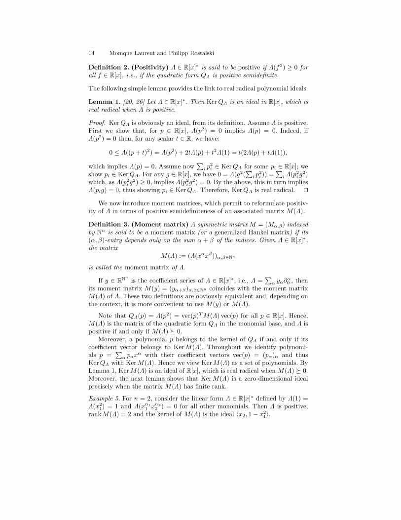
Example 5. For n = 2, consider the linear form Λ ∈ R[x]∗ defined by Λ(1) =Λ(x21) = 1 and Λ(xα1
1 xα22 ) = 0 for all other monomials. Then Λ is positive,
rankM(Λ) = 2 and the kernel of M(Λ) is the ideal 〈x2, 1− x21〉.
The Approach of Moments for Polynomial Equations 15
Lemma 2. Let Λ ∈ R[x]∗ and let B be a set of monomials. Then, B indexesa maximal linearly independent set of columns of M(Λ) if and only if B cor-responds to a basis of R[x]/KerM(Λ). That is,
rankM(Λ) = dimR[x]/KerM(Λ).
Next we collect some properties of the moment matrix of evaluations atpoints of Rn.
Lemma 3. If Λ = Λv is the evaluation at v ∈ Rn, then M(Λv) = [v]∞[v]T∞has rank 1 and its kernel is I(v), the vanishing ideal of v. More generally, if Λis a conic combination of evaluations at real points, say Λ =
∑ri=1 λiΛvi where
λi > 0 and vi ∈ Rn are pairwise distinct, then M(Λ) =∑ri=1 λi[vi]∞[vi]
T∞
has rank r and its kernel is I(v1, . . . , vr), the vanishing ideal of the vi’s.
The following theorem of Curto and Fialkow [7] shows that any positivelinear form Λ with a finite rank moment matrix is a conic combination ofevaluations at real points. In other words, it shows that the implication ofLemma 3 holds as an equivalence. This result will play a crucial role in ourapproach. We give a proof, based on [20], although some details are simplified.
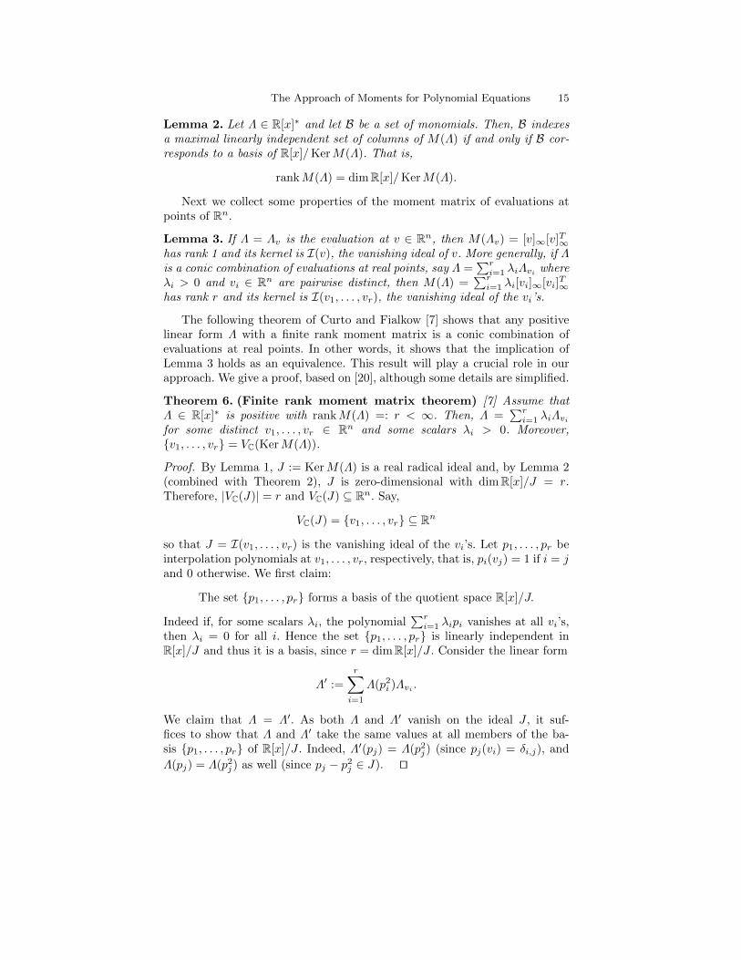
Theorem 6. (Finite rank moment matrix theorem) [7] Assume thatΛ ∈ R[x]∗ is positive with rankM(Λ) =: r < ∞. Then, Λ =
∑ri=1 λiΛvi
for some distinct v1, . . . , vr ∈ Rn and some scalars λi > 0. Moreover,{v1, . . . , vr} = VC(KerM(Λ)).
Proof. By Lemma 1, J := KerM(Λ) is a real radical ideal and, by Lemma 2(combined with Theorem 2), J is zero-dimensional with dimR[x]/J = r.Therefore, |VC(J)| = r and VC(J) ⊆ Rn. Say,
VC(J) = {v1, . . . , vr} ⊆ Rn
so that J = I(v1, . . . , vr) is the vanishing ideal of the vi’s. Let p1, . . . , pr beinterpolation polynomials at v1, . . . , vr, respectively, that is, pi(vj) = 1 if i = jand 0 otherwise. We first claim:
The set {p1, . . . , pr} forms a basis of the quotient space R[x]/J.
Indeed if, for some scalars λi, the polynomial∑ri=1 λipi vanishes at all vi’s,
then λi = 0 for all i. Hence the set {p1, . . . , pr} is linearly independent inR[x]/J and thus it is a basis, since r = dimR[x]/J . Consider the linear form
Λ′ :=
r∑i=1
Λ(p2i )Λvi .
We claim that Λ = Λ′. As both Λ and Λ′ vanish on the ideal J , it suf-fices to show that Λ and Λ′ take the same values at all members of the ba-sis {p1, . . . , pr} of R[x]/J . Indeed, Λ′(pj) = Λ(p2j ) (since pj(vi) = δi,j), and
Λ(pj) = Λ(p2j ) as well (since pj − p2j ∈ J). ut
16 Monique Laurent and Philipp Rostalski
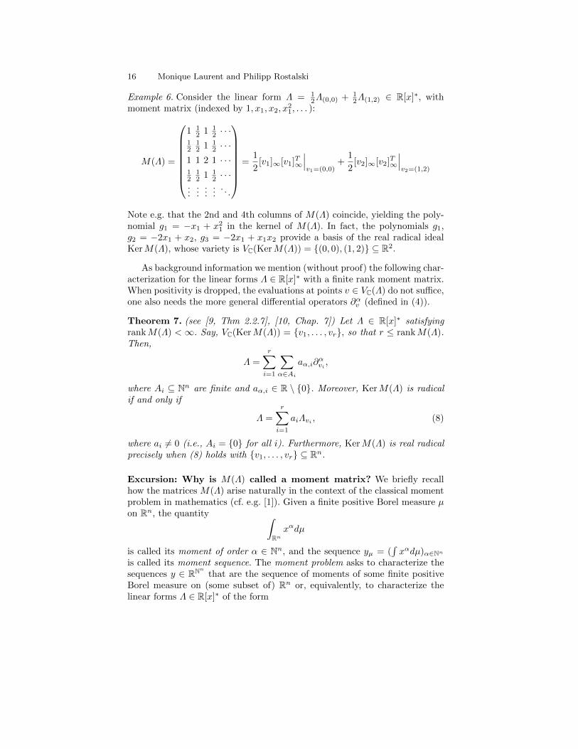
Example 6. Consider the linear form Λ = 12Λ(0,0) + 1
2Λ(1,2) ∈ R[x]∗, withmoment matrix (indexed by 1, x1, x2, x
21, . . . ):
M(Λ) =
1 12 1 1
2 · · ·12
12 1 1
2 · · ·1 1 2 1 · · ·12
12 1 1
2 · · ·...
......
.... . .
=
1
2[v1]∞[v1]T∞
∣∣∣v1=(0,0)
+1
2[v2]∞[v2]T∞
∣∣∣v2=(1,2)
Note e.g. that the 2nd and 4th columns of M(Λ) coincide, yielding the poly-nomial g1 = −x1 + x21 in the kernel of M(Λ). In fact, the polynomials g1,g2 = −2x1 + x2, g3 = −2x1 + x1x2 provide a basis of the real radical idealKerM(Λ), whose variety is VC(KerM(Λ)) = {(0, 0), (1, 2)} ⊆ R2.
As background information we mention (without proof) the following char-acterization for the linear forms Λ ∈ R[x]∗ with a finite rank moment matrix.When positivity is dropped, the evaluations at points v ∈ VC(Λ) do not suffice,one also needs the more general differential operators ∂αv (defined in (4)).
Theorem 7. (see [9, Thm 2.2.7], [10, Chap. 7]) Let Λ ∈ R[x]∗ satisfyingrankM(Λ) < ∞. Say, VC(KerM(Λ)) = {v1, . . . , vr}, so that r ≤ rankM(Λ).Then,
Λ =
r∑i=1
∑α∈Ai
aα,i∂αvi ,
where Ai ⊆ Nn are finite and aα,i ∈ R \ {0}. Moreover, KerM(Λ) is radicalif and only if
Λ =
r∑i=1
aiΛvi , (8)
where ai 6= 0 (i.e., Ai = {0} for all i). Furthermore, KerM(Λ) is real radicalprecisely when (8) holds with {v1, . . . , vr} ⊆ Rn.
Excursion: Why is M(Λ) called a moment matrix? We briefly recallhow the matrices M(Λ) arise naturally in the context of the classical momentproblem in mathematics (cf. e.g. [1]). Given a finite positive Borel measure µon Rn, the quantity ∫
Rn
xαdµ
is called its moment of order α ∈ Nn, and the sequence yµ = (∫xαdµ)α∈Nn
is called its moment sequence. The moment problem asks to characterize thesequences y ∈ RNn
that are the sequence of moments of some finite positiveBorel measure on (some subset of) Rn or, equivalently, to characterize thelinear forms Λ ∈ R[x]∗ of the form
The Approach of Moments for Polynomial Equations 17
Λ = Λµ(p) :=
∫p(x)dµ for p ∈ R[x]. (9)
When (9) holds, µ is called a representing measure for Λ. A well known re-sult of Haviland [11] claims that Λ has a representing measure if and only ifΛ(p) ≥ 0 for all polynomials p that are nonnegative on Rn. However, exceptin some exceptional cases3 no characterization is known for the nonnegativepolynomials on Rn. Yet we find the following well known necessary condition:If Λ has a representing measure, then Λ(p2) ≥ 0 for all polynomials p, i.e., Λis positive, which is characterized by M(Λ) � 0.
Positivity of Λ is in general only a necessary condition for existence of arepresenting measure. However, the above result of Curto and Fialkow (The-orem 6) shows equivalence in the case when M(Λ) has finite rank, in whichcase the measure µ is finite atomic with support VC(KerM(Λ)).
When µ = δv is the Dirac measure at a point v ∈ Rn, its moment sequenceis yµ = [v]∞ with corresponding linear form Λµ = Λv, the evaluation at v.More generally, when µ is finitely atomic, i.e., of the form µ =
∑ri=1 λiδvi
with finite support {v1, . . . , vr} ⊆ Rn, then its moment sequence is yµ =∑ri=1 λi[vi]∞ with corresponding linear form Λµ =
∑ri=1 λiΛvi .
Characterizing real radical ideals using positive linear forms on R[x].We now combine the above results to obtain a semidefinite characterizationof real radical ideals using positive linear forms. For this define the convex set
K = {Λ ∈ R[x]∗ |Λ(1) = 1,M(Λ) � 0 and Λ(p) = 0 ∀p ∈ I} . (10)
For any Λ ∈ K, KerM(Λ) is a real radical ideal, which contains I and thusits real radical R
√I. This implies:
dimR[x]/KerM(Λ) ≤ dimR[x]/R√I.
When the real variety VR(I) is finite, R[x]/ R√I has finite dimension as a vector
space, equal to |VR(I)|, and thus KerM(Λ) is zero-dimensional with
rankM(Λ) = dimR[x]/KerM(Λ) ≤ dimR[x]/R√I = |VR(I)|
(using Lemma 2 for the left most equality). Equality: rankM(Λ) = |VR(I)|holds, for instance, for the element Λ = 1
|VR(I)|∑v∈VR(I)
Λv of K. This fact
motivates the following definition:
3 A celebrated result of Hilbert (cf. e.g. [2]) shows that there are three sets ofparameters (n, d) for which the following equivalence holds: For any polynomialp in n variables and degree 2d, p is nonnegative on Rn if and only if p can bewritten as a sum of squares of polynomials. These parameters are (n = 1, d)(univariate polynomials), (n, d = 1) (quadratic polynomials), and (n = 3, d = 2)(ternary quartic polynomials). In all other cases there are polynomials that arenonnegative on Rn but cannot be written as a sum of squares of polynomials.
18 Monique Laurent and Philipp Rostalski
Definition 4. (Generic linear forms) Let K be defined as in (10) and as-sume |VR(I)| < ∞. A linear form Λ ∈ K is said to be generic if M(Λ) hasmaximum rank, i.e., if rankM(Λ) = |VR(I)|.
A simple geometric property of positive semidefinite matrices yields thefollowing equivalent definition for generic elements of K. This is in fact thekey tool used in [17] for computing the real radical ideal R
√I.
Lemma 4. Assume |VR(I)| < ∞. An element Λ ∈ K is generic if and onlyif KerM(Λ) ⊆ KerM(Λ′) for all Λ′ ∈ K. Moreover, KerM(Λ) = R
√I for all
generic Λ ∈ K.
Proof. Assume first that rankM(Λ) = r, with r = |VR(I)| and VR(I) ={v1, . . . , vr}. As Λ+ Λ′ ∈ K for Λ′ ∈ K, we have
KerM(Λ+ Λ′) = KerM(Λ) ∩KerM(Λ′) ⊆ KerM(Λ),
implying r ≥ rankM(Λ+Λ′) ≥ rankM(Λ). Hence equality holds throughoutwhich implies KerM(Λ) = KerM(Λ) ∩KerM(Λ′) ⊆ KerM(Λ′).
Conversely, assume KerM(Λ) ⊆ KerM(Λ′) for all Λ′ ∈ K. ConsiderΛ′ =
∑ri=1 Λvi ∈ K whose kernel is I(v1, . . . , vr). This implies KerM(Λ) ⊆
I(v1, . . . , vr) and thus
rankM(Λ) = dimR[x]/KerM(Λ) ≥ dimR[x]/I(v1, . . . , vr) = r.
Hence, rankM(Λ) = r and KerM(Λ) = I(v1, . . . , vr) = R√I (using the Real
Nullstellensatz, Theorem 1 (ii), for the last equality). ut
Example 7 (Example 6 cont.). Consider the set K corresponding to the idealI = 〈h1, h2, h3〉 ⊆ R[x1, x2], where
h1 = x42x1 + 3x31 − x42 − 3x21, h2 = x21x2 − 2x21, h3 = 2x42x1 − x31 − 2x42 + x21.
Then, Λ = 12Λ(0,0) + 1
2Λ(1,2) is a generic element of K. Thus the real radical
ideal of I is R√I = KerM(Λ) = 〈g1, g2, g3〉, with g1, g2, g3 as in Example 6.
3.2 Truncated positive linear forms and real radical ideals
In view of the results in the previous section (in particular, Lemmas 2 and 4),the task of finding the real radical ideal R
√I as well as a linear basis of the
quotient space R[x]/ R√I can be reduced to finding a generic linear form Λ
in the set K (defined in (10)). In order to be able to deal with such linearforms computationally, we will work with linear forms on finite dimensionalsubspaces R[x]s of the polynomial ring. Given Λ ∈ (R[x]2s)
∗, we can definethe quadratic form:
QΛ : f ∈ R[x]s 7→ QΛ(f) = Λ(f2),
The Approach of Moments for Polynomial Equations 19
whose matrixMs(Λ) = (Λ(xαxβ))α,β∈Nn
s
in the monomial basis of R[x]s is called the truncated moment matrix of order sof Λ. Thus Λ is positive (i.e., Λ(f2) ≥ 0 ∀f ∈ R[x]s) if and only if Ms(Λ) � 0.Again we identify the kernels of QΛ and of Ms(Λ) (by identifying polynomialswith their coefficient sequences) and view KerMs(Λ) as a subset of R[x]s.
Flat extensions of moment matrices. We now present the following cru-cial result of Curto and Fialkow [7] for flat extensions of moment matrices.
Theorem 8. (Flat extension theorem) ([7], see also [21]) Let Λ ∈ (R[x]2s)∗
and assume that Ms(Λ) is a flat extension of Ms−1(Λ), i.e.,
rankMs(Λ) = rankMs−1(Λ). (11)
Then one can extend (uniquely) Λ to Λ ∈ (R[x]2s+2)∗ in such a way thatMs+1(Λ) is a flat extension of Ms(Λ); thus rankMs+1(Λ) = rankMs(Λ).
The proof is elementary and relies on the following lemma showing that thekernel of a truncated moment matrix behaves like a ‘truncated ideal’.
Lemma 5. Let Λ ∈ (R[x]2s)∗ and f, g ∈ R[x] with f ∈ KerMs(Λ).
(i) Assume rankMs(Λ) = rankMs−1(Λ). Then KerMs−1(Λ) ⊆ KerMs(Λ)and fg ∈ KerMs(Λ) if deg(fg) ≤ s.
(ii) Assume Ms(Λ) � 0. Then KerMs−1(Λ) ⊆ KerMs(Λ) and fg ∈ KerMs(Λ)if deg(fg) ≤ s− 1.
Indeed, using property (11) and Lemma 5 (i), we see that for every monomialm of degree s, there exists a polynomial of the form fm = m+rm ∈ KerMs(Λ),where rm ∈ R[x]s−1. If an extension Λ exists, then all the polynomialsfm, xifm must lie in the kernel of Ms+1(Λ) and they can be used to de-termine the unknown columns of Ms+1(Λ) indexed by monomials of degrees+1. The main work consists of verifying the consistency of this construction;namely, that the matrix constructed in this way is a moment matrix, i.e. thatits (α, β)th entry depends only on the sum α+β when |α+β| = 2s+1, 2s+2.
The flat extension theorem plays a crucial role in the moment matrixapproach as it allows to deduce information about the infinite moment matrixM(Λ) from its finite section Ms(Λ).
Theorem 9. [17] Let Λ ∈ (R[x]2s)∗ and assume that (11) holds. Then one can
extend Λ to Λ ∈ R[x]∗ in such a way that M(Λ) is a flat extension of Ms(Λ),and the ideal KerM(Λ) is generated by the polynomials in KerMs(Λ), i.e.,
rankM(Λ) = rankMs(Λ) and KerM(Λ) = 〈KerMs(Λ)〉.
Moreover, any monomial set B indexing a basis of the column space ofMs−1(Λ) is a basis of the quotient space R[x]/KerM(Λ). If, moreover,Ms(Λ) � 0, then the ideal 〈KerMs(Λ)〉 is real radical and Λ is of the formΛ =
∑ri=1 λiΛvi , where λi > 0 and {v1, . . . , vr} = VC(KerMs(Λ)) ⊆ Rn.
20 Monique Laurent and Philipp Rostalski
Proof. The existence of Λ follows by applying iteratively Theorem 8 and theinclusion 〈KerMs(Λ)〉 ⊆ KerM(Λ) follows using Lemma 5 (i). If B is a set ofmonomials indexing a column basis of Ms−1(Λ), then B is also a column basisof M(Λ) and thus a basis of R[x]/KerM(Λ) (by Lemma 2). One can verifythe direct sum decomposition R[x] = SpanR(B)⊕ 〈KerMs(Λ)〉, which impliesKerM(Λ) = 〈KerMs(Λ)〉. Finally, as Λ is a flat extension of Λ, Ms(Λ) �0 implies M(Λ) � 0, so that 〈KerMs(Λ)〉 = KerM(Λ) is real radical (byLemma 1). The final statement follows directly by applying Theorem 6 to Λ.ut
Example 8 (Example 6 cont.). Consider the linear form Λ ∈ R[x]∗ in Exam-ple 6. Recall that KerM(Λ) is generated by g1, g2, g3 ∈ R[x]2. First note thatthese polynomials imply the rank condition: rankM2(Λ) = rankM1(Λ) andthus permit to construct M2(Λ) from M1(Λ). Moreover, they permit to re-cover the infinite matrix M(Λ) from its submatrix M1(Λ). For instance, sincex21x2 = x2(x1 +g1) = 2x1 +g3 +g1x2 and g1, g2, g3 ∈ KerM2(Λ) ⊆ KerM(Λ),we deduce that the column of M(Λ) indexed by x21x2 is equal to twice itscolumn indexed by x1. Using the fact that KerM(Λ) = 〈KerM2(Λ)〉 , we cananalogously define iteratively all columns of M(Λ).
Computing real radical ideals using truncated positive linear formson R[x]t. We saw above how to use positive linear forms on R[x] to charac-terize the real radical ideal R
√I. We now combine this characterization with
the above results about flat extensions of truncated moment matrices to ob-tain a practical algorithm for computing R
√I operating on finite dimensional
subspaces R[x]t ⊆ R[x] only. As before I = 〈h1, . . . , hm〉 is the ideal generatedby the polynomial equations hi to be solved. For t ∈ N, define the set
Ht = {hixα | i = 1, . . . ,m, |α| ≤ t− deg(hi)} (12)
of prolongations up to degree t of the polynomials hi, and the truncatedanalogue of the set K:
Kt = {Λ ∈ (R[x]t)∗ | Λ(1) = 1, Mbt/2c(Λ) � 0 and Λ(f) = 0 ∀f ∈ Ht}. (13)
Note that the constraint: Λ(f) = 0 ∀f ∈ Ht (i.e., Λ ∈ H⊥t ) corresponds tothe constraint (2) of Section 1.2. As the convex set Kt is described by thepositive semidefiniteness of an affinely parametrized matrix, it is an instanceof a spectrahedron, cf. Chapter ??? of this volume. The following lemma is thetruncated analogue of Lemma 4.
Lemma 6. (Generic truncated linear forms) The following assertionsare equivalent for Λ ∈ (R[x]t)
∗:
(i) rankMbt/2c(Λ) ≥ rankMbt/2c(Λ′) for all Λ′ ∈ Kt.
(ii) KerMbt/2c(Λ) ⊆ KerMbt/2c(Λ′) for all Λ′ ∈ Kt.
(iii)The linear form Λ lies in the relative interior of the convex set Kt.
The Approach of Moments for Polynomial Equations 21
Then Λ is called a generic element of Kt and the kernel Nt = KerMbt/2c(Λ)is independent of the particular choice of the generic element Λ ∈ Kt.
Theorem 10. We have: Nt ⊆ Nt+1 ⊆ . . . ⊆ R√I, with equality R
√I = 〈Nt〉 for
t large enough.
Proof. Let Λ ∈ Kt+1 be generic. Its restriction to (R[x]t)∗ lies in Kt, implying
Nt+1 = KerMb(t+1)/2c(Λ) ⊇ KerMbt/2c(Λ) ⊇ Nt.
Now let Λ be a generic element of Kt so that Nt = KerMbt/2c(Λ). The in-clusion: Nt ⊆ I(VR(I)) follows using Lemma 6 (ii). Indeed, Λv ∈ Kt for allv ∈ VR(I), which implies KerMbt/2c(Λ) ⊆ KerMbt/2c(Λv) ⊆ I(v) and thus
KerMbt/2c(Λ) ⊆⋂
v∈VR(I)
I(v) = I(VR(I)) =R√I (by the Real Nullstellensatz).
We now show equality: R√I = 〈Nt〉 for t large enough. For this, let
{g1, . . . , gL} be a basis of the ideal R√I; we show that gl ∈ Nt for all l. We
have:
g2kl +∑j
s2j =
m∑i=1
uihi for some k ∈ N and sj , ui ∈ R[x].
Since Λ ∈ H⊥t , we have hi ∈ Nt if t ≥ 2 deg(hi). Using Lemma 5 (ii), thisimplies that, for t large enough, Nt contains each uihi and thus g2kl +
∑j s
2j .
In particular, Λ(g2kl +∑j s
2j ) = 0. On the other hand, Λ(g2kl ), Λ(s2j ) ≥ 0
(since Mbt/2c(Λ) � 0), thus implying Λ(g2kl ) = 0. An easy induction on k nowpermits to conclude that gl ∈ Nt. ut
When VR(I) is finite, one can guaranty the equality R√I = 〈Nt〉 using the
rank condition (11). The next results provide all the ingredients of the mo-ment matrix algorithm for real roots, whose description is given in Section3.3: Theorem 11 will provide a stopping criterion (when |VR(I)| < ∞) andTheorem 12 below will imply its termination, as well as provide a criterionpermitting to check the (non-)existence of real roots.
Theorem 11. [17] Let I = 〈h1, . . . , hm〉 be an ideal in R[x], D = maxi deg(hi),and d = dD/2e. Let Λ ∈ Kt be a generic element and assume that at least oneof the following two conditions holds:
rankMs(Λ) = rankMs−1(Λ) for some D ≤ s ≤ bt/2c, (14)
rankMs(Λ) = rankMs−d(Λ) for some d ≤ s ≤ bt/2c. (15)
Then, R√I = 〈KerMs(Λ)〉, and any basis of the column space of Ms−1(Λ) is
a basis of the quotient space R[x]/ R√I.
Proof. The ideal J := 〈KerMs(Λ)〉 is real radical (by Theorem 9). Moreover,
KerMs(Λ) ⊆ KerMbt/2c(Λ) ⊆ R√I
22 Monique Laurent and Philipp Rostalski
(since Λ is generic and using Theorem 10) and thus J ⊆ R√I. Remains to show
R√I ⊆ J . Suppose first that (14) holds. The condition Λ ∈ H⊥t implies that
hi ∈ KerMs(Λ) (since s + deg(hi) ≤ t/2 + deg(hi) ≤ t, as t ≥ 2D). ThusI ⊆ J , implying R
√I ⊆ J as J is real radical.
Suppose now that (15) holds. Again from Theorem 9 we know thatVC(KerMs(Λ)) = {v1, . . . , vr} ⊆ Rn and Λ =
∑ri=1 λiΛvi where λi > 0. Let
p1, . . . , pr be interpolation polynomials at the vi’s, i.e., such that pj(vi) = δi,j .An easy but crucial observation (made in [20]) is that we may assume thateach pj has degree at most s − d. Indeed, we can replace each interpolationpolynomial pj by its normal form modulo J with respect to a basis of R[x]/J .As such a basis can be obtained by picking a column basis of Ms−d(Λ), itsmembers are monomials of degree at most s − d, and the resulting normalforms of the pj ’s are again interpolation polynomials at the vi’s but now withdegree at most s−d. As deg(p2j ) ≤ 2(s−d) ≤ t−2d ≤ t−deg(hi), we can claim
that Λ(p2jhi) = 0 and in turn 0 = Λ(p2jhi) =∑rl=1 λlp
2j (vl)hi(vl) = λjhi(vj).
Since hi(vj) = 0 for all i, j, we conclude that {v1, . . . , vr} ⊆ VR(I), implying
the desired inclusion R√I = I(VR(I)) ⊆ I(v1, . . . , vr) = J . ut
Theorem 12. [17] Let I be an ideal in R[x].
(i) If VR(I) = ∅, then Kt = ∅ for t large enough.(ii) If 1 ≤ |VR(I)| <∞ then, for t large enough, there exists an integer s for
which (15) holds for all Λ ∈ Kt.
Proof. Let {g1, . . . , gL} be a Grobner basis of R√I with respect to a total degree
monomial ordering, and let B be the corresponding set of standard monomials,forming a basis of R[x]/ R
√I. The argument used in the proof of Theorem 10
shows the existence of t0 ∈ N for which {g1, . . . , gL} ⊆ KerMbt/2c(Λ) for allt ≥ t0 and Λ ∈ Kt.(i) If VR(I) = ∅, then {1} is a basis of R
√I = R[x]. Thus 1 ∈ KerMbt/2c(Λ),
implying Λ(1) = 0 if Λ ∈ Kt, contradicting Λ(1) = 1 and thus showingKt = ∅.(ii) As VR(I) is finite, s := d + maxb∈B deg(b) is well defined. Recall thatd = maxiddeg(hi)/2e. Choose t ≥ t0 such that s < bt/2c. For α ∈ Nns ,decompose xα as
xα =∑b∈B
λbb+
L∑l=1
ulgl ∈ SpanR(B)⊕ R√I,
where λb ∈ R, ul ∈ R[x], deg(∑b λbb) ≤ s − d, and deg(ulgl) ≤ s < bt/2c
(as the gl’s form a Grobner basis for a total degree ordering, we can claimdeg(ulgl) ≤ s). As gl ∈ KerMbt/2c(Λ) and deg(ulgl) < bt/2c, we also havethat ulgl ∈ KerMbt/2c(Λ) (recall Lemma 5 (ii)). Hence, xα −
∑b∈B λbb ∈
KerMbt/2c(Λ), which shows that Ms(Λ) is a flat extension of Ms−d(Λ). ut
Example 9 (Example 7 cont.). Consider again the ideal I = (h1, h2, h3) fromExample 7. Then, D = 5, dimR[x]/I = 9, and the variety VC(I) consists of
The Approach of Moments for Polynomial Equations 23
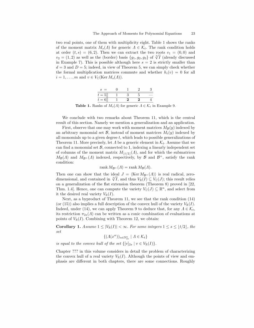
two real points, one of them with multiplicity eight. Table 1 shows the ranksof the moment matrix Ms(Λ) for generic Λ ∈ Kt. The rank condition holdsat order (t, s) = (6, 2). Then we can extract the two roots v1 = (0, 0) andv2 = (1, 2) as well as the (border) basis {g1, g2, g3} of R
√I (already discussed
in Example 7). This is possible although here s = 2 is strictly smaller thand = 3 and D = 5; indeed, in view of Theorem 5, we can simply check whetherthe formal multiplication matrices commute and whether hi(v) = 0 for alli = 1, . . . ,m and v ∈ VC(KerMs(Λ)).
s = 0 1 2 3
t = 5 1 3 5 —
t = 6 1 2 2 4
Table 1. Ranks of Ms(Λ) for generic Λ ∈ Kt in Example 9.
We conclude with two remarks about Theorem 11, which is the centralresult of this section. Namely we mention a generalization and an application.
First, observe that one may work with moment matrices MB(y) indexed byan arbitrary monomial set B, instead of moment matrices Mt(y) indexed byall monomials up to a given degree t, which leads to possible generalizations ofTheorem 11. More precisely, let Λ be a generic element in Kt. Assume that wecan find a monomial set B, connected to 1, indexing a linearly independent setof columns of the moment matrix Mbt/2c(Λ), and for which the submatricesMB(Λ) and MB+(Λ) indexed, respectively, by B and B+, satisfy the rankcondition:
rankMB+(Λ) = rankMB(Λ).
Then one can show that the ideal J = 〈KerMB+(Λ)〉 is real radical, zero-dimensional, and contained in R
√I, and thus VR(I) ⊆ VC(J); this result relies
on a generalization of the flat extension theorem (Theorem 8) proved in [22,Thm. 1.4]. Hence, one can compute the variety VC(J) ⊆ Rn, and select fromit the desired real variety VR(I).
Next, as a byproduct of Theorem 11, we see that the rank condition (14)(or (15)) also implies a full description of the convex hull of the variety VR(I).Indeed, under (14), we can apply Theorem 9 to deduce that, for any Λ ∈ Kt,its restriction π2s(Λ) can be written as a conic combination of evaluations atpoints of VR(I). Combining with Theorem 12, we obtain:
Corollary 1. Assume 1 ≤ |VR(I)| <∞. For some integers 1 ≤ s ≤ bt/2c, theset
{(Λ(xα))α∈Nn2s| Λ ∈ Kt}
is equal to the convex hull of the set {[v]2s | v ∈ VR(I)}.
Chapter ??? in this volume considers in detail the problem of characterizingthe convex hull of a real variety VR(I). Although the points of view and em-phasis are different in both chapters, there are some connections. Roughly
24 Monique Laurent and Philipp Rostalski
speaking, both chapters can be cast within the more general realm of polyno-mial optimization (see Section 4.1); however, while we work here with trun-cated sections of the ideal I, Chapter ??? deals with linear forms on the fullquotient space R[x]/I.
3.3 The moment matrix algorithm for computing real roots
We now describe the moment matrix algorithm for computing real roots,summarized in Algorithm 1 below.
Algorithm 1 The moment matrix algorithm for VR(I)
Input: Generators h1, . . . , hm of some ideal I = 〈h1, . . . , hm〉 with |VR(I)| <∞.Output: A basis of the ideal R√I, a basis of R[x]/ R√I, and the set VR(I).1: Set t = D.2: Find a generic element Λ ∈ Kt.3: Check if (14) holds for some D ≤ s ≤ bt/2c,
or if (15) holds for some d ≤ s ≤ bt/2c.4: if yes then5: Set J = 〈KerMs(Λ)〉.6: Compute a basis B ⊆ R[x]s−1 of the column space of Ms−1(Λ).7: Compute the multiplication matrices Xi in R[x]/J .8: Compute a basis g1, . . . , gl ∈ R[x]s of the ideal J .9: return the basis B of R[x]/J and the generators g1, . . . , gl of J .
10: else11: Iterate (go to Step 2) replacing t by t+ 1.12: end if13: Compute VR(I) = VC(J) (via the eigenvalues/eigenvectors of the multiplication
matrices Xi).
Theorem 11 implies the correctness of the algorithm (i.e., equality J = R√I)
and Theorem 12 shows its termination. Algorithm 1 consists of four mainparts, which we now briefly discuss (see [17, 36] for details).
(i) Finding a generic element in Kt. The set Kt can be represented asthe feasible region of a semidefinite program and we have to find a pointlying in its relative interior. Such a point can be found by solving severalsemidefinite programs with an arbitrary SDP solver (cf. [17, Remark 4.15]),or by solving a single semidefinite program with an interior-point algorithmusing a self-dual embedding technique (see, e.g., [8], [45]). Indeed consider thesemidefinite program:
minΛ∈(R[x]t)∗
1 such that Λ(1) = 1, Mbt/2c(Λ) � 0,
Λ(hixα) = 0 ∀i ∀|α| ≤ t− deg(hi),
(16)
whose dual reads:

The Approach of Moments for Polynomial Equations 25
maxλ such that 1− λ = s+∑mi=1 uihi where s, ui ∈ R[x],
s is a sum of squares, deg(s),deg(uihi) ≤ t.(17)
The feasible region of (16) is the set Kt, as well as its set of optimal solutions,since we minimize a constant objective function over Kt. There is no dualitygap, as λ = 1 is obviously feasible for (17). Solving the program (16) with aninterior-point algorithm using a self-dual embedding technique yields4 eithera solution Λ lying in the relative interior of the optimal face (i.e., a genericelement of Kt), or a certificate that (16) is infeasible thus showing VR(I) = ∅.
(ii) Computing the ranks of submatrices of Mt(Λ). In order to checkwhether one of the conditions (14) or (15) holds we need to compute the ranksof matrices consisting of numerical values. This computationally challengingtask may be done by detecting zero singular values and/or a large decaybetween two subsequent values.
(iii) Computing a basis B for the column space of Ms−1(Λ). The set ofmonomials B indexing a maximum nonsingular principle submatrix of Ms(Λ)directly reveals a basis of the quotient space R[x]/J (by Theorem 9). Thechoice of this basis may influence the numerical stability of the extracted setof solutions and the properties of the border basis of J as well. The optionsrange from a monomial basis obtained using a greedy algorithm or more so-phisticated polynomial bases (see [36]).
(iv) Computing a basis of J and the formal multiplication matrices.Say B is the monomial basis (connected to 1) of the column space of Ms−1(Λ)constructed at the previous step (iii). Under the rank condition (14) or (15),for any b ∈ B, the monomial xib can be written as xib = ri,b + q, where ri,b ∈SpanR(B) and q ∈ KerMs(Λ). These polynomials directly give a (border)basis of J , consisting of the polynomials {xib − ri,b | i ≤ n, b ∈ B} (recallTheorem 5) and thus permit the construction of multiplication matrices andthe computation of VC(J) (= VR(I)).
Existing implementations and performance. The basic algorithm dis-cussed above has been implemented in Matlab using Yalmip (see [25]) as partof a new toolbox Bermeja for computations in Convex Algebraic Geometry(see [37]). In its current form, the implemented algorithm merely provides aproof of concept and only solves real root finding problems with a rather lim-ited number of variables (≤ 10) and of moderate degree (≤ 6). This is mainlydue to the fact that sparsity in the support of the polynomials is not utilized.This leads to large moment matrices, easily touching on the limitations ofcurrent SDP solver. We refer to [17, 19] for a more detailed discussion andsome numerical results. In an ongoing project a more efficient, Buchberger-style, version of this real root finding method will be implemented based onthe more general version of the flat extension theorem, which was described at
4 This follows under certain technical conditions on the semidefinite program, whichare satisfied for (16); see [17] for details.
26 Monique Laurent and Philipp Rostalski
the end of Section 3.2. A flavor of how existing complex root finding methodsmay be tailored for real root finding is discussed in the next section.
3.4 Real vs. complex root finding
As we saw in the previous section, the moment matrix approach for real rootsrelies on finding a suitable (generic) linear form Λ in the convex set Kt (from(13)). Let us stress again that the positivity condition on Λ is the essentialingredient that permits to focus solely on the real roots among the complexones. This is best illustrated by observing (following [18]) that, if we delete thepositivity condition in the moment matrix algorithm (Algorithm 1), then thesame algorithm permits to compute all complex roots (assuming their numberis finite). In other words, consider the following analogue of the set Kt:
KCt = {Λ ∈ (R[x]t)
∗ |Λ(1) = 1 and Λ(f) = 0 ∀f ∈ Ht} , (18)
where Ht is as in (12). Call an element Λ ∈ KCt generic5 if rankMs(Λ) is
maximum for all s ≤ bt/2c. Then the moment matrix algorithm for complexroots is analogous to Algorithm 1, but with the following small twist: Insteadof computing a generic element in the convex set Kt, we have to computea generic (aka random) element in the affine space KC
t , thus replacing thesemidefinite feasibility problem by a linear algebra computation. We refer to[18] for details on correctness and termination of this algorithm.
Alternatively one can describe the above situation as follows: the com-plex analogue of Algorithm 1 is an algorithm for complex roots, which canbe turned into an algorithm for real roots simply by adding the positiv-ity condition on Λ. This suggests that the same recipe could be applied toother algorithms for complex roots. This is indeed the case, for instance, forthe prolongation-projection algorithm of [35] which, as shown in [19], can beturned into an algorithm for real roots by adding a positivity condition. Thealgorithm of [35] works with the space KC
t but uses a different stopping crite-rion instead of the rank condition (14). Namely one should check whether, forsome D ≤ s ≤ t, the three affine spaces πs(KC
t ), πs−1(KCt ), and πs(KC
t+1) havethe same dimensions (where πs(Λ) denotes the restriction of Λ ∈ (R[x]t)
∗ to(R[x]s)
∗); if so, one can compute a basis of R[x]/I and extract VC(I). Roughlyspeaking, to turn this into an algorithm for real roots, one adds positivity andconsiders the convex set Kt instead of KC
t ; again one needs to check thatthree suitably defined spaces have the same dimensions; if so, then one canextract VR(I). We refer to [19] for details, also about the links between therank condition and the above alternative stopping criterion.
5 When Λ is positive, the maximality condition on the rank of Mbt/2c(Λ) impliesthat the rank of Ms(Λ) is maximum for all s ≤ bt/2c. This is not true for Λnon-positive.
The Approach of Moments for Polynomial Equations 27
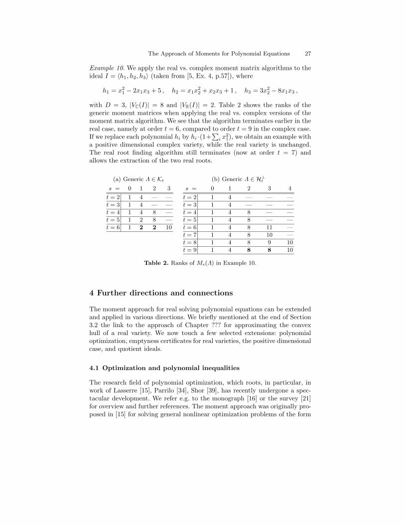
Example 10. We apply the real vs. complex moment matrix algorithms to theideal I = 〈h1, h2, h3〉 (taken from [5, Ex. 4, p.57]), where
h1 = x21 − 2x1x3 + 5 , h2 = x1x22 + x2x3 + 1 , h3 = 3x22 − 8x1x3 ,
with D = 3, |VC(I)| = 8 and |VR(I)| = 2. Table 2 shows the ranks of thegeneric moment matrices when applying the real vs. complex versions of themoment matrix algorithm. We see that the algorithm terminates earlier in thereal case, namely at order t = 6, compared to order t = 9 in the complex case.If we replace each polynomial hi by hi ·(1+
∑i x
21), we obtain an example with
a positive dimensional complex variety, while the real variety is unchanged.The real root finding algorithm still terminates (now at order t = 7) andallows the extraction of the two real roots.
(a) Generic Λ ∈ Kt
s = 0 1 2 3
t = 2 1 4 — —
t = 3 1 4 — —
t = 4 1 4 8 —
t = 5 1 2 8 —
t = 6 1 2 2 10
(b) Generic Λ ∈ H⊥ts = 0 1 2 3 4
t = 2 1 4 — — —
t = 3 1 4 — — —
t = 4 1 4 8 — —
t = 5 1 4 8 — —
t = 6 1 4 8 11 —
t = 7 1 4 8 10 —
t = 8 1 4 8 9 10
t = 9 1 4 8 8 10
Table 2. Ranks of Ms(Λ) in Example 10.
4 Further directions and connections
The moment approach for real solving polynomial equations can be extendedand applied in various directions. We briefly mentioned at the end of Section3.2 the link to the approach of Chapter ??? for approximating the convexhull of a real variety. We now touch a few selected extensions: polynomialoptimization, emptyness certificates for real varieties, the positive dimensionalcase, and quotient ideals.
4.1 Optimization and polynomial inequalities
The research field of polynomial optimization, which roots, in particular, inwork of Lasserre [15], Parrilo [34], Shor [39], has recently undergone a spec-tacular development. We refer e.g. to the monograph [16] or the survey [21]for overview and further references. The moment approach was originally pro-posed in [15] for solving general nonlinear optimization problems of the form
28 Monique Laurent and Philipp Rostalski
f∗ = minx
f(x) such that h1(x) = 0, . . . , hm(x) = 0,
g1(x) ≥ 0, . . . , gp(x) ≥ 0,(19)
where f, hi, gj ∈ R[x]. Let I = 〈h1, . . . , hm〉 be the ideal generated by the hi’s,and set
S = {x ∈ Rn | g1(x) ≥ 0, . . . , gp(x) ≥ 0}, (20)
so that (19) asks to minimize f over the semi-algebraic set VR(I) ∩ S. Thebasic observation in [15] is that the problem (19) can be reformulated as
minµ
Λµ(f) such that µ is a probability measure on VR(I) ∩ S,
where Λµ is as in (9). Such a linear form satisfies: Λ(h) = 0 for all h ∈ I, as wellas the positivity condition: Λ(gjf
2) ≥ 0 for all f ∈ R[x] and j = 1, . . . , p. Thelatter conditions can be reformulated as requiring that the localizing momentmatrices M
bt−deg(gj)
2 c(gjΛ) be positive semidefinite. Here, for g ∈ R[x], gΛ is
the new linear form defined by gΛ(p) = Λ(pg) for all p ∈ R[x].The semidefinite program (16) can be modified in the following way to
yield a relaxation of (19):
f∗t = minΛ∈(R[x]t)∗
Λ(f) such that Λ(1) = 1, Λ(h) = 0 ∀h ∈ Ht,
Mbt−deg(gj)
2 c(gjΛ) � 0 (j = 0, 1, . . . , p)
(21)
(setting g0 = 1). The dual semidefinite program reads:
max λ such that f − λ =
p∑j=0
σjgj +
m∑i=1
uihi (22)
where ui ∈ R[x], σj are sums of squares of polynomials with deg(uihi),deg(σjgj) ≤ t. Then, f∗t ≤ f∗ for all t. Moreover, asymptotic convergenceof (21) and (22) to the minimum f∗ of (19) can be shown when the feasi-ble region of (19) is compact and satisfies some additional technical condition(see [15]). We now group some results showing finite convergence under certainrank condition, which can be seen as extensions of Theorems 11 and 12.
Theorem 13. [12, 17, 21] Let D := maxi,j(deg(hi),deg(gj)), d := dD/2e,t ≥ max(deg(f), D), and let Λ be a generic optimal solution to (21) (i.e., forwhich rankMbt/2c(Λ) is maximum), provided it exists.
(i) If the rank condition (15) holds with 2s ≥ deg(f), then f∗t = f∗ andVC(KerMs(Λ)) is equal to the set of global minimizers of the program (19).
(ii) If VR(I) is nonempty and finite, then (15) holds with 2s ≥ deg(f).(iii)If VR(I) = ∅, then the program (21) is infeasible for t large enough.
The Approach of Moments for Polynomial Equations 29
In other words, under the rank condition (15), one can compute all globalminimizers of the program (19), since, as before, one can compute a basisof the space R[x]/〈KerMs(Λ)〉 from the moment matrix and thus apply theeigenvalue method. Moreover, when the equations hi = 0 have finitely manyreal roots, the rank condition is guaranteed to hold after finitely many steps.
By choosing the constant objective function f = 1 in (19), we can alsocompute the S-radical ideal:
S√I := I(VR(I) ∩ S).
When |VR(I)| is nonempty and finite, one can show that
I(VR(I) ∩ S) = 〈KerMs(Λ)〉
for a generic optimal solution Λ of (21) and s, t large enough. An analogousresult holds under the weaker assumption that |VR(I) ∩ S| is nonempty andfinite. In this case Λ needs to be a generic feasible solution of the modifiedsemidefinite program obtained by adding to (21) the positivity conditions:
Mb t−deg(g)2 c(gΛ) � 0 for g = ge11 · · · gepp ∀e ∈ {0, 1}p.
The key ingredient in the proof is to use the Positivstellensatz to characterizethe polynomials in I(VR(I) ∩ S) (see [42]) instead of the Real Nullstellensatz(used in Theorem 10 to characterize the polynomials in I(VR(I))).
Let us illustrate on an example how to ‘zoom in’ on selected roots, by in-corporating semi-algebraic constraints or suitably selecting the cost function.
Example 11. Consider the following system, known as Katsura 5 (see [13]):
h1 = 2x26 + 2x25 + 2x24 + 2x23 + 2x22 + x21 − x1 ,h2 = x6x5 + x5x4 + 2x4x3 + 2x3x2 + 2x2x1 − x2 ,h3 = 2x6x4 + 2x5x3 + 2x4x2 + x22 + 2x3x1 − x3 ,h4 = 2x6x3 + 2x5x2 + 2x3x2 + 2x4x1 − x4 ,h5 = x23 + 2x6x1 + 2x5x1 + 2x4x1 − x5 ,h6 = 2x6 + 2x5 + 2x4 + 2x3 + 2x2 + x1 − 1,
with D = 2, |VC(I)| = 32, and |VR(I)| = 12. Table 3(a) shows the ranks ofthe generic moment matrices for the moment matrix algorithm to computeVR(I). At order (t, s) = (6, 3), the algorithm finds all twelve real roots.
Next we apply the moment matrix algorithm to compute the real roots inS = {x ∈ R6 | g(x) = x1 − 0.5 ≥ 0}; the ranks are shown in Table 3(b) andall five elements of VR(I) ∩ S can be computed at order (t, s) = (4, 2).
If we are interested e.g. only in the roots in VR(I) ∩ S with the small-est x2-coordinate then we minimize the polynomial x2 (instead of the con-stant one polynomial). The moment matrix algorithm now terminates at or-der (t, s) = (2, 1) and finds the unique element of VR(I)∩ S with the smallestx2-coordinate.
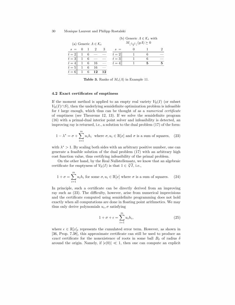
30 Monique Laurent and Philipp Rostalski
(a) Generic Λ ∈ Kt
s = 0 1 2 3
t = 2 1 6 — —
t = 3 1 6 — —
t = 4 1 6 16 —
t = 5 1 6 16 —
t = 6 1 6 12 12
(b) Generic Λ ∈ Kt withMb t−1
2c(gΛ) � 0
s = 0 1 2
t = 2 1 6 —
t = 3 1 6 —
t = 4 1 5 5
Table 3. Ranks of Ms(Λ) in Example 11.
4.2 Exact certificates of emptiness
If the moment method is applied to an empty real variety VR(I) (or subsetVR(I)∩S), then the underlying semidefinite optimization problem is infeasiblefor t large enough, which thus can be thought of as a numerical certificateof emptiness (see Theorems 12, 13). If we solve the semidefinite program(16) with a primal-dual interior point solver and infeasibility is detected, animproving ray is returned, i.e., a solution to the dual problem (17) of the form:
1− λ∗ = σ +
m∑i=1
uihi where σ, ui ∈ R[x] and σ is a sum of squares, (23)
with λ∗ > 1. By scaling both sides with an arbitrary positive number, one cangenerate a feasible solution of the dual problem (17) with an arbitrary highcost function value, thus certifying infeasibility of the primal problem.
On the other hand, by the Real Nullstellensatz, we know that an algebraiccertificate for emptyness of VR(I) is that 1 ∈ R
√I, i.e.,
1 + σ =
m∑i=1
uihi for some σ, ui ∈ R[x] where σ is a sum of squares. (24)
In principle, such a certificate can be directly derived from an improvingray such as (23). The difficulty, however, arise from numerical imprecisionsand the certificate computed using semidefinite programming does not holdexactly when all computations are done in floating point arithmetics. We maythus only derive polynomials ui, σ satisfying
1 + σ + ε =
m∑i=1
uihi, (25)
where ε ∈ R[x]t represents the cumulated error term. However, as shown in[36, Prop. 7.38], this approximate certificate can still be used to produce anexact certificate for the nonexistence of roots in some ball Bδ of radius δaround the origin. Namely, if |ε(0)| � 1, then one can compute an explicit
The Approach of Moments for Polynomial Equations 31
δ for which one can prove that VR(I) ∩ Bδ = ∅. This is illustrated on thefollowing example.
Example 12. Consider the ideal I = 〈h1, h2, h3〉 generated by
h1 = x41 + x42 + x43 − 4 , h2 = x51 + x52 + x53 − 5 , h3 = x61 + x62 + x63 − 6
with D = 6, |VC(I)| = 120, and VR(I) = ∅. At order t = 6 already, the primal(moment) problem is infeasible, the solver returns an improving directionfor the dual (SOS) problem, and we obtain a numerical certificate of theform (25). The error polynomial ε ∈ R[x] is a dense polynomial of degree 6,its coefficients are smaller than 4.1e-11, with constant term ε(0) < 8.53e-14.Using the conservative estimate of [36, §7.8.2] one can rigorously certify theemptiness of the set VR(I) ∩ Bδ for δ = 38.8. In other words, even if we onlysolved the problem numerically with a rather low accuracy, we still obtain aproof that the ideal I does not have any real root v ∈ VR(I) with ‖v‖2 < 38.8.By increasing the accuracy of the SDP solver the radius δ of the ball can befurther increased. This example illustrates that it is sometimes possible todraw exact conclusions from numerical computations.
4.3 Positive dimensional ideals and quotient ideals
Dealing with positive dimensional varieties is a challenging open problem,already for complex varieties (see e.g. the discussion in [24]). The algorithmpresented so far for computing the real variety VR(I) and the real radicalideal R
√I works under the assumption that VR(I) is finite. Indeed, the rank
condition (14) (or (15)) implies that dimR[x]/ R√I = rankMs−1(Λ) is finite (by
Theorem 11). Nevertheless, the moment method can in principle be appliedto find a basis of R
√I also in the positive dimensional case. Indeed Theorem 10
shows that, for t large enough, the kernel of Mbt/2c(Λ) (for generic Λ ∈ Kt)generates the real radical ideal R
√I. The difficulty however is that it is not
clear how to recognize whether equality R√I = 〈KerMbt/2c(Λ)〉 holds in the
positive dimensional case. These questions relate in particular to the studyof the Hilbert function of R
√I (see [36]). An interesting research direction is
whether the moment matrix approach can be applied to compute some form of“parametric representation” of the real variety. On some instances it is indeedpossible to compute parametric multiplication matrices (see [36] for details).
Another interesting object is the quotient (or colon) ideal
I : g = {p ∈ R[x] | pg ∈ I}
for an ideal I and g ∈ R[x]. The moment approach can be easily adapted to
find a semidefinite characterization of the ideal R√I : g = I
(VR(I) \ VR(g)
).
Indeed, for generic Λ, the kernel of the localizing moment matrix of gΛ carriesall information about this ideal.
32 Monique Laurent and Philipp Rostalski
Proposition 1. Let g ∈ R[x]k, ρ := 1 + dk/2e and D = maxi deg(hi). Let Λbe a generic element in Kt+k.
(i) 〈KerMbt/2c(gΛ)〉 ⊆ R√I : g, with equality for t large enough.
(ii) If the rank condition: rankMs(Λ) = rankMs−ρ(Λ) holds for some s with
max(D, ρ) ≤ s ≤ bt/2c, then R√I : g = 〈KerMs−ρ+1(gΛ)〉.
(iii)If VR(I) is nonempty finite, then the rank condition in (ii) holds at someorder (t, s).
Proof. Note that p ∈ KerMbt/2c(gΛ) if and only if pg ∈ KerMbt/2c(Λ) whendeg(p) ≤ bt/2c − k.(i) As Λ is generic, KerMbt/2c(Λ) ⊆ R
√I, implying 〈KerMbt/2c(gΛ)〉 ⊆ R
√I : g.
The proof of equality for t large enough is similar to the proof of Theorem 10:Pick a basis {g1, . . . , gL} of the ideal R
√I : g, so that each glg belongs to R
√I;
apply the Real Nullstellensatz to glg to conclude that, for t large enough,glg ∈ KerMbt/2c(Λ) and thus gl ∈ KerMbt/2c(gΛ).(ii) Assume now rankMs(Λ) = rankMs−ρ(Λ) for D, ρ ≤ s ≤ bt/2c. Then
there exists Λ ∈ R[x]∗ for which M(Λ) is a flat extension of Ms(Λ) andR√I = KerM(Λ) = 〈KerMs−ρ+1(Λ)〉 (use Theorems 9 and 11). Therefore,
R√I : g = KerM(Λ) : g = KerM(gΛ). One can verify that M(gΛ) is a flat
extension of Ms−ρ(gΛ), which implies that KerM(gΛ) = 〈KerMs−ρ+1(gΛ)〉(using Theorem 9) is thus equal to 〈KerMs−ρ+1(gΛ)〉 (since Λ and Λ coincideon R[x]2s).(iii) follows from an easy modification of the proof of Theorem 12. ut
We conclude this chapter with a small example on quotient ideals.
Example 13. Consider I = 〈x2 − x21, x22 − x2〉, with roots (0, 0) (double) and(±1, 1), and R
√I = 〈x2−x21, x22−x2, x1x2−x1〉. The quotient ideal computation
with g = x1 terminates at order (t, s) = (6, 3) and we obtain that R√I : g is
generated by x2 − x21, x2 − 1, with variety VR(I) \ VR(g) = {(−1, 1), (1, 1)}.The corresponding ranks of Ms(Λ) and Ms(gΛ) are shown in Table 4.
(a) rankMs(Λ)
s = 0 1 2 3
t = 4 1 3 3 —
t = 5 1 3 3 —
t = 6 1 3 3 3
(b) rankMs(gΛ)
s = 0 1 2 3
t = 4 1 2 — —
t = 5 1 2 — —
t = 6 1 2 2 —
Table 4. Rank sequences for generic Λ ∈ Kt in Example 13.
The Approach of Moments for Polynomial Equations 33
References
1. N.I. Akhiezer, The Classical Moment Problem, Hafner, 1965.2. S. Basu, R. Pollack, and M.F. Roy, Algorithms in Real Algebraic Geometry,
Springer, 2003.3. D. Bates and F. Sottile, Khovanskii-Rolle continuation for real solutions,
arXiv:0908.4579, 2009.4. J. Bochnak, M. Coste, and M.-F. Roy, Real Algebraic Geometry, Springer, 1998.5. D.A. Cox, J.B. Little, and D.B. O’Shea, Using Algebraic Geometry, Springer,
1998.6. , Ideals, Varieties, and Algorithms : An Introduction to Computational
Algebraic Geometry and Commutative Algebra, Springer, 2005.7. R.E. Curto and L. Fialkow, Solution of the truncated complex moment prob-
lem for flat data, Memoirs of the American Mathematical Society 119 (1996),no. 568, 1–62.
8. E. de Klerk, Aspects of Semidefinite Programming - Interior Point Algorithmsand Selected Applications, Kluwer, 2002.
9. A. Dickenstein and I. Z. Emiris (eds.), Solving Polynomial Equations: Founda-tions, Algorithms, and Applications, Algorithms and Computation in Mathe-matics, vol. 14, Springer, 2005.
10. M. Elkadi and B. Mourrain, Introduction a la Resolution des Systemesd’Equations Polynomiaux, Mathematiques et Applications, vol. 59, Springer,2007.
11. E.K. Haviland, On the momentum problem for distribution functions in morethan one dimension. II, American Journal of Mathematics 58 (1936), no. 1,164–168.
12. D. Henrion and J.B. Lasserre, Detecting global optimality and extracting solu-tions in GloptiPoly, In Positive Polynomials in Control, Lecture Notes in Controland Information Sciences, pp. 293–310, Springer, 2005.
13. http://www.mat.univie.ac.at/~neum/glopt/coconut/Benchmark/
Library3/katsura5.mod
14. A. Kehrein and M. Kreuzer, Characterizations of border bases, Journal of Pureand Applied Algebra 196 (2005), 251–270.
15. J.B. Lasserre, Global optimization with polynomials and the problem of moments,SIAM Journal on Optimization 11 (2001), 796–817.
16. , Moments, Positive Polynomials, and their Applications, Imperial Col-lege Press, 2009.
17. J.B. Lasserre, M. Laurent, and P. Rostalski, Semidefinite characterization andcomputation of real radical ideals, Foundations of Computational Mathematics8 (2008), no. 5, 607–647.
18. , A unified approach for real and complex zeros of zero-dimensional ide-als., In Emerging Applications of Algebraic Geometry (M. Putinar and S. Sulli-vant, eds.), vol. 149, Springer, 2009, pp. 125–156.
19. , A prolongation-projection algorithm for computing the finite real varietyof an ideal, Theoretical Computer Science 410 (2009), no. 27-29, 2685–2700.
20. M. Laurent, Revisiting two theorems of Curto and Fialkow, Proceedings of theAmerican Mathematical Society 133 (2005), no. 10, 2965–2976.
21. , Sums of squares, moment matrices and optimization over polynomials,In Emerging Applications of Algebraic Geometry (M. Putinar and S. Sullivant,eds.), Springer, 2009, pp. 157–270.
34 Monique Laurent and Philipp Rostalski
22. M. Laurent and B. Mourrain, A generalized flat extension theorem for momentmatrices, Archiv der Mathematik 93 (2009), no. 1, 87–98.
23. D. Lazard, Resolution des systemes d’equations algebriques, Theoretical Com-puter Science 15 (1981), 77–110.
24. , Thirty years of polynomial system solving, and now? Journal of Sym-bolic Computation 44 (2009), 222-231.
25. J. Lofberg, YALMIP: A Toolbox for Modeling and Optimization in MATLAB,Computer Aided Control Systems Design Conference (Taipei, Taiwan), 2004,Available from http://users.isy.liu.se/johanl/yalmip/.
26. H.M. Moller, An inverse problem for cubature formulae, Computational Tech-nologies 9 (2004), 13–20.
27. T. Mora, Solving Polynomial Equation Systems I: The Kronecker-Duval Phi-losophy, Encyclopedia of Mathematics and its Applications, no. 88, CambridgeUniversity Press, 2003.
28. , Solving Polynomial Equation Systems II: Macaulay’s Paradigm andGrobner Technology, Encyclopedia of Mathematics and its Applications (v. 2),no. 88, Cambridge University Press, 2005.
29. B. Mourrain, A new criterion for normal form algorithms, AAECC, LectureNotes in Computer Science, pp. 430–443, 1999.
30. , Pythagore’s dilemma, symbolic - numeric computation and the bor-der basis method, In Symbolic-numeric computation, Trends in Mathematics,pp. 223–243, Birkhauser, 2007.
31. B. Mourrain and J. P. Pavone, Subdivision methods for solving polynomial equa-tions, Journal of Symbolic Computation 44 (2009), no. 3, 292–306.
32. B. Mourrain and P. Trebuchet, Generalized normal forms and polynomials sys-tem solving, In Proc. Intern. Symp. on Symbolic and Algebraic Computation(M. Kauers, ed.), pp. 253-260, ACM Press, 2005.
33. B. Mourrain, J.B. Lasserre, M. Laurent, P. Rostalski and P. Trebuchet, Momentmatrices and border bases, In preparation.
34. P.A. Parrilo, Structured Semidefinite Programs and Semialgebraic GeometryMethods in Robustness and Optimization, Ph.D. thesis, California Institute ofTechnology, 2000.
35. G. Reid and L. Zhi, Solving polynomial systems via symbolic-numeric reductionto geometric involutive form, Journal of Symbolic Computation 44 (2009), no. 3,280 – 291.
36. P. Rostalski, Algebraic Moments – Real Root Finding and Related Topics, Ph.D.thesis, ETH Zurich, 2009.
37. , Bermeja: Convex Algebraic Geometry in MATLAB, Available fromhttp://math.berkeley.edu/~philipp/cagwiki.
38. F. Rouillier, Solving zero-dimensional systems through the rational univariaterepresentation, Journal of Applicable Algebra in Engineering, Communicationand Computing 9 (1999), no. 5, 433–461.
39. N.Z. Shor, An approach to obtaining global extremums in polynomial mathemat-ical programming problems, Kibernetica 5 (1987), 102–106.
40. A.J. Sommese and C.W. Wampler, The Numerical Solution of Systems of Poly-nomials Arising in Engineering and Science, World Scientific Press, 2005.
41. F. Sottile, Numerical real algebraic geometry, In preparation, 2009.42. G. Stengle, A Nullstellensatz and a Positivstellensatz in semialgebraic geometry,
Mathematische Annalen 207 (1974), 87–97.
The Approach of Moments for Polynomial Equations 35
43. H.J. Stetter, Numerical Polynomial Algebra, SIAM, 2004.44. B. Sturmfels, Solving Systems of Polynomial Equations, American Mathematical
Society, 2002.45. H. Wolkowicz, R. Saigal, and L. Vandenberghe (eds.), Handbook of Semidefinite
Programming: Theory, Algorithms, and Applications, vol. 27, Kluwer AcademicPublishers, Dordrecht, The Netherlands / Boston, MA, 2000.