The application of GIS based decision-tree models for ... · R. Bou Kheir et al.: GIS tree modeling of organic wet landscapes 849 25 1 Fig. 1. Soil map of the study area within Denmark

Hydrol. Earth Syst. Sci., 14, 847–857, 2010www.hydrol-earth-syst-sci.net/14/847/2010/doi:10.5194/hess-14-847-2010© Author(s) 2010. CC Attribution 3.0 License.

Hydrology andEarth System

Sciences

The application of GIS based decision-tree models for generatingthe spatial distribution of hydromorphic organic landscapes inrelation to digital terrain data

R. Bou Kheir, P. K. Bøcher, M. B. Greve, and M. H. Greve

Department of Agroecology and Environment, Faculty of Agricultural Sciences (DJF), Aarhus University, Blichers Alle 20,P.O. Box 50, 8830 Tjele, Denmark

Received: 21 December 2009 – Published in Hydrol. Earth Syst. Sci. Discuss.: 18 January 2010Revised: 11 May 2010 – Accepted: 17 May 2010 – Published: 1 June 2010

Abstract. Accurate information about organic/mineral soiloccurrence is a prerequisite for many land resources man-agement applications (including climate change mitigation).This paper aims at investigating the potential of using geo-morphometrical analysis and decision tree modeling to pre-dict the geographic distribution of hydromorphic organiclandscapes in unsampled area in Denmark. Nine primary(elevation, slope angle, slope aspect, plan curvature, pro-file curvature, tangent curvature, flow direction, flow accu-mulation, and specific catchment area) and one secondary(steady-state topographic wetness index) topographic param-eters were generated from Digital Elevation Models (DEMs)acquired using airborne LIDAR (Light Detection and Rang-ing) systems. They were used along with existing digitaldata collected from other sources (soil type, geological sub-strate and landscape type) to explain organic/mineral fieldmeasurements in hydromorphic landscapes of the Danisharea chosen. A large number of tree-based classificationmodels (186) were developed using (1) all of the parame-ters, (2) the primary DEM-derived topographic (morpholog-ical/hydrological) parameters only, (3) selected pairs of pa-rameters and (4) excluding each parameter one at a time fromthe potential pool of predictor parameters. The best classifi-cation tree model (with the lowest misclassification error andthe smallest number of terminal nodes and predictor parame-ters) combined the steady-state topographic wetness indexand soil type, and explained 68% of the variability in or-ganic/mineral field measurements. The overall accuracy ofthe predictive organic/inorganic landscapes’ map produced(at 1:50 000 cartographic scale) using the best tree was esti-

Correspondence to:R. Bou Kheir([email protected])

mated to be ca. 75%. The proposed classification-tree modelis relatively simple, quick, realistic and practical, and it canbe applied to other areas, thereby providing a tool to facil-itate the implementation of pedological/hydrological plansfor conservation and sustainable management. It is particu-larly useful when information about soil properties from con-ventional field surveys is limited.

1 Introduction

Detailed soil spatial information is indispensable for land re-sources management and environmental modeling. Distribu-tion patterns of organic/mineral soil occurence have a largepotential to affect global climate, and the international effortsfor using soils and vegetation as carbon sinks are rapidly in-creasing (IPCC, 2000). Changes in soil organic distributionare attributed to both natural processes and human activities,the latter being widely recognized in recent years. Land usechanges, including deforestation, biomass burning, drainingof wetlands (being usually humus-rich), ploughing, use offertilizers and other agricultural practices, are regarded asthe main factors causing loss of soil organic carbon (SOC)and the emission of CO2 into the atmosphere. These changescan be significant in hydromorphic grasslands and croplandswhere intensive artificial drainage activities are carried out.This is particularly true in the case of Denmark with an im-portant reduction of the total wetland area during the past200 years as a result of much drainage activity (digging ofdrainage ditches and introduction of tile drainage).

As part of international efforts to stabilize atmosphericgreenhouse gas concentrations, Denmark (like severalother countries) is committed to establish inventories of

Published by Copernicus Publications on behalf of the European Geosciences Union.

http://creativecommons.org/licenses/by/3.0/

848 R. Bou Kheir et al.: GIS tree modeling of organic wet landscapes

organic/mineral soil distribution in the frame of Kyoto proto-col. Modeling tools of diverse soil properties (including or-ganic/mineral soil occurence) require more information thanavailable even in detailed soil maps. Digital Soil Mappinghas been tested in a wide range of soil mapping contextsat different scales throughout the world (McBratney et al.,2003; Dobos et al., 2006; Grunwald, 2006). It has beenused to understand and quantify the relationships betweensoils and their environmental attributes, mostly derived fromexhaustive and easy-to-access datasets such as Digital Eleva-tion Models (DEMs) and remote sensing imagery. Accordingto Bishop and Minasny (2005) and McBratney et al. (2003),in almost 80% of digital soil mapping projects DEMs areused as the most important data source to derive landformsand run predictions of soil properties. Topographic attributescontrol the differential distribution of water, sediments, anddissolved material, which in turn result in soil differentiation(Pachepsky et al., 2001).

Soil landscape modeling has been successfully applied topredict soil variability in small landscapes of less than 100ha (Moore et al., 1993; Gessler et al., 2000; Florinsky etal., 2002). These studies have demonstrated that combina-tions of one to five terrain attributes derived from DEMs canexplain 20 to 88% of the variability of selected soil prop-erties. The empirical relationships between soil propertiesand terrain attributes are unique to each soil property andeach soil-forming environment. Recent soil landscape pre-dictive algorithms such as neural networks, fuzzy logic ortree model tools arose mainly from data-mining and machinelearning fields, also referred to as knowledge discovery in adatabase in its overall process (Fayyad et al., 1996). Soillandscape prediction from existing maps involves recoveringthe mental model used by the soil surveyor to set up the map(Lagacherie et al., 1995; Bui, 2004). This is a reverse soilmapping process and has broad relevance to any other appli-cation of knowledge discovery from natural resource maps(Qi and Zhu, 2003). Many researchers have utilized otherstatistical methods, such as multiple regression, stepwise re-gression, stepwise principal component regression, and cor-relation analysis to study the relationships between DEM-derived terrain attributes and different soil attributes, but inmost cases for specific, localized landscapes (Moore et al.,1993; Dobos et al., 2000; Gessler et al., 2000; Egli et al.,2006a; Hengl, 2009).

Classification tree analysis (CTA) is a modeling tech-nique that is being used increasingly (Henderson et al., 2004;Lawrence et al., 2004), being dedicated to the prediction ofcategorical data (classes of soil properties). It significantlyenhances the ability of the DEM-derived variables to predictsoil attributes (e.g. organic/mineral soil occurrence). CTAhas several advantages that seem to suit well soil-landscapemodelling applications. One of the most interesting featuresis that they are non-parametric, which means that no assump-tion is made regarding variable distribution (Breiman, 2001).Thus, it avoids variable transformation caused, for instance,

by bi-modal or skewed histograms, which are frequent insoil class signatures (Lawrence et al., 2004). They are non-sensitive to missing data, perform automatic variable subsetselection, are not sensitive to the inclusion of a large numberof irrelevant variables, and finally, they can handle quanti-tative and categorical data, making it possible to integrateDEM-derived variables and indexes together with geologyor soil categorical layers (Breiman, 2001; Henderson et al.,2004; Lawrence et al., 2004). However, in the built clas-sification trees, the uncertainties of the classes in each oneof their leaves can be explored. Efficiency of using CTAfor predictive soil landscape mapping was demonstrated ina few studies at regional and subregional scale (Moran andBui, 2002; Scull et al., 2005). Recent studies showed theirpotential for land cover mapping from remote sensing imagesanalysis (Friedl et al., 1999; Lawrence et al., 2004), geomor-phological mapping (Luoto and Hjort, 2005) and soil erosionoccurrence (Bou Kheir et al., 2008).

As mentioned by Luoto and Hjort (2005), CTA was prac-tically used in two linked but distinct purposes: inductionand prediction. Induction-oriented studies used CTA to un-cover the relationship between soil units or properties andenvironmental attributes, to identify the discriminant vari-ables and to compare rules determined by the model with ex-pert knowledge-based rules (McKenzie and Ryan, 1999; Buiet al., 2006). On the other hand, prediction-oriented stud-ies used quantitative relationships between the soil responsevariables and the environmental soil-forming factors to pre-dict soil landscape patterns over unvisited areas (Lagacherieet al., 1995; Moran and Bui, 2002; Scull et al., 2005).

The purpose of this study is to implement CTA and eval-uate its ability to provide accurate soil landscape predictionand more precisely to determine the geographic distributionof hydromorphic organic landscapes (target variable beingthe organic/mineral soil occurence) depending on the exist-ing field surveys’ data collected during the last 60 years atan unsampled area in Denmark from mapped environmen-tal variables. Our hypothesis was that spatial patterns of or-ganic ditribution in hydromorphic landscapes could be pre-dicted from spatial patterns of terrain attributes that havebeen shown to influence soil-forming processes. Predictionof hydromorphic organic landscapes will have implicationsfor the proper management of marginal and environmentallysensitive areas. Understanding how soil organic distributionvaries across landscape positions based on limited field sam-ples has become the focal point of much environmental re-search nowadays.

2 Study area description

The chosen study area, covering about 1812 km2, is locatedin southern Denmark (Fig. 1). It has been selected dueto the strong link between land use on historical maps andsoil internal drainage (Dalsgaard, 1997), which induces the

Hydrol. Earth Syst. Sci., 14, 847–857, 2010 www.hydrol-earth-syst-sci.net/14/847/2010/

R. Bou Kheir et al.: GIS tree modeling of organic wet landscapes 849

25

1

Fig. 1. Soil map of the study area within Denmark (Madsen et al., 1992).

accumulation of organic carbon on poorly drained Danishsoils (Madsen et al., 1992). The climate is temperate withmean annual temperature ranging from 0 to 16◦C, and aWest-East gradient in precipitation oscillating between 900and 600 mm/year (1961–1990). 95% of parent materialshave glacial and fluvio-glacial origin. Approximately 65%of these materials were deposited during the last glacial pe-riod (between 10 000 and 100 000 years), and 20% duringthe previous glacial period (more than 110 000 years ago).However, the deposits from that period were all strongly re-distributed by periglacial processes, and evidence of earliersoil formations is extremely rare. The area is representativeof a broad region of landscapes in Denmark (i.e. Weichselmoraine landscape, Glacifluvial plains, Saalian landscape,Aeolian landscape, and Post glacial marine deposits). Theelevation varies from 0 m in the western part to 85 m in theeastern part. The area has been intensively cropped since theMiddle Ages. Currently, 70% of the area is cultivated, 10%forested and the rest urbanized.

3 Materials and methods

The spatial prediction of hydromorphic organic landscapeswas realized in several steps, combining existing soil sur-vey collection, geomorphometrical analysis and decision tree

modeling. Some existing field surveys were collected forspecifying organic soils at visited locations. The obtainedfield samples’ layer information (point location) was thenintersected with maps of predictor parameters (as extractedfrom DEMs and other sources). A large number of un-prunedand pruned classification-tree models (186) were explored onthe result of this intersection combining field samples loca-tions and the corresponding parameters. The best tree modelwith the lowest misclassification error and the lowest num-ber of terminal nodes and predictor parameters was used forproducing a predictive map of organic/inorganic landscapes’map within the hydromorphic landscapes of the study areausing GIS (Geographic Information Systems).

3.1 Soil samples collection and analysis

The soil was sampled at 1541 sites selected by four differ-ent existing field surveys to be representative for the area.In order to avoid soil variability on a small scale, 25 bulksoil samples were taken within a radius of 50 m from a depthof 0–30 cm (plough layer) in the Danish Soil Classification(1975) and the Danish Profile Investigation (1990). The col-lected samples in these two existing surveys were taken to thelaboratory for analysis. These samples were air-dried at roomtemperature and passed through a 2 mm soil sieve. Concen-trations of soil organic carbon (SOC) were determined by the

www.hydrol-earth-syst-sci.net/14/847/2010/ Hydrol. Earth Syst. Sci., 14, 847–857, 2010


combustion method in a LECO induction furnace, convertedto % Soil Organic Matter (SOM) using a factor of 1.72. Theother two surveys (ochre classification and well database per-formed in 1985) gave categorical information on parent ma-terial (e.g. peat, sand, silt and clay). This parent material in-formation was reclassified into organic and mineral soils. Inorder to increase the number of samples used in the modelingprocess, the continuous soil organic matter (SOM) obtainedin the former surveys was converted to a categorical variable(organic/mineral soil occurence) using 10% SOM as a cutoff value (commonly used in Denmark). With less than 10%SOM, soils are classified as mineral; and with more than 10%SOM, soils are considered organic.

3.2 Geomorphometrical analysis

It has been postulated in several studies that the occurrence ofhydromorphic organic landscapes is dictated by topographicfeatures of the landscape (Moore et al., 1993; Gessler et al.,1995; Bou Kheir et al., 2007). In this study, we considereasy to derive and interpret terrain parameters from DigitalElevation Models.

3.2.1 Generation of Digital Elevation Model

A digital elevation model (DEM) was generated for the cho-sen area from airborne LIDAR (Light Detection and Rang-ing) systems. The latter seem effective and reliable means ofterrain data collection in relatively large areas with cloudyweather conditions (Baltsavias, 1999; Brian et al., 2007;Schmitt et al., 2007; Liu, 2008). The established triangularirregular network (TIN) was converted using a TOPOGRIDalgorithm to an ArcGIS grid of 1.6-m pixel resolution. Thisresolution was chosen to match the planimetric and altimetricaccuracies of LIDAR systems. In order to increase the effi-ciency in terms of storage and manipulation, and to acquirehomogeneity and standardization with used ancillary maps,the constructed high-resolution DEM was coarsened in thisstudy to 25-m resolution.

The produced elevation surface (DEM) would still containseveral spurious elements, usually classified either as sinksor peaks (one or two cells below or above the local surface).The errors vary between 0.1 m and 4.7 m in a typical 25 mDEM (Tarboton et al., 1991). Although many authors agreethat sinks and peaks may actually represent the true nature oftopography (Chorowicz et al., 1992), they may act as localbarriers that trap water flow and cause a major problem fordrainage network extraction. To avoid this problem and be-fore performing any hydrologic analysis, sinks in the DEMwere identified and eliminated using TerraStream software(Danner et al., 2007).

3.2.2 Derivation of morphological/hydrological param-eters from Digital Elevation Model

The chosen morphological/hydrological predictor parame-ters may aid spatial estimation of hydromorphic organiclandscapes, because the relief had a great influence on soilformation and its physical/chemical properties (McKenzieand Ryan, 1999; Bou Kheir et al., 2007, 2008). They may bedivided into primary and compound attributes. In this study,the nine primary parameters, i.e. elevation, slope angle, slopeaspect, plan curvature, profile curvature, tangent curvature,flow direction, flow accumulation, and specific catchmentarea were directly derived from the constructed Digital Ele-vation Model (DEM) using specific TerraSTREAM (Danneret al., 2007) and ArcGIS (version 9.3) algorithms.

Elevation is useful for classifying the local relief, andlocating points of maximum and minimum heights. Ithad a high correlation with organic/mineral soil occurence(Thompson and Kolka, 2005). At regional scales, several au-thors found that soil organic carbon content increased withelevation over ranges of≥1000 m, since lower temperaturescharacterize higher elevations (Bolstad et al., 2001; Egli etal., 2003, 2006b).

Slope,S, characterizing the spatial rate of change of eleva-tion in the direction of steepest descent, affects the velocityof both surface and subsurface flow, and hence the water andorganic carbon contents in landscapes.

As for slope aspect,ψ (orientation of the line of steep-est descent), is useful for visualizing hydromorphic or-ganic landscapes, and is frequently recorded in pedologi-cal/hydrological surveys. Aspect is divided into the eightmajor directions plus the non-oriented flat areas. Slopes ex-posed to the south and west are more subject to runoff fortwo reasons: (1) they are warmer with higher evaporationrates and lower moisture storage capacity, thus less forestedthan those exposed to the north and east, and (2) rainfall af-fects slope aspect depending on the direction of winds duringrainfall, which commonly has a west and south–west trend inDenmark.

Slope curvature,K, measures the distribution of convexand concave areas; hence the propensity of water to con-verge or diverge as it flows across the land. Convex sur-faces are most likely to be well drained, while for concavesurfaces depressions have a higher likelihood of having hy-dromorphic features. Concave slopes can concentrate morewater and sediments indicating the potential accumulationof a large quantity of organic soils. Convex slopes showan inverse effect, dispersing flow and limiting material ac-cumulation, therefore a lesser quantity of soil tends to accu-mulate than on concave slopes. Flat areas (zero curvature)are without any effect on flow divergence or convergence.Curvature attributes (plan, profile and tangent) are based onsecond derivatives: the rate of change of a first derivativesuch as slope gradient or slope aspect, usually in a particular



direction. Curvatures were derived through GIS from theconstructed DEM.

The type and the amount of soil organic carbon (SOC) arestrongly related to the presence of water. The drainage net-work provides an important indication of water percolationrate. Special hydrological algorithms were used dependingon known matrices (i.e. flow direction matrix, flow accumu-lation and stream network) to derive the drainage networkrunning over the study area (Tarboton et al., 1991; Chorow-icz et al., 1992). A stream network was derived by connect-ing all pixels that accumulate flow from 100 pixels or more.Flow accumulation grid and digitized outlets from the streamnetwork were used to automatically subdivide the whole areainto small watersheds. Each watershed was subdivided intotwo facets, separated by the streamline passing through thewatershed.

The specific catchment area, representing the upslope areaper unit width of contour, was calculated using the finite dif-ference slope algorithm and FD8 flow-routing method witha maximum area of 50 000 m2. FD8 was chosen becauseit allows flow to be distributed to multiple nearest neighbornodes in upland areas above different channels, thus model-ing flow divergence using flow dispersion. It takes consider-ably longer to run than the more common D8 algorithm butit avoids many of the problems incurred with D8 and givesmuch more realistic distributions of contributing area (Gal-lant and Wilson, 2000).

In addition to primary terrain attributes, a compound to-pographic index (CTI), often referred to as the steady-statewetness index was also calculated for each pixel using theaverage upslope contributing area (As) and the slope degree(β), according to the formula (CTI=ln [As/tanβ]) (Moore etal., 1993; Wilson and Gallant, 2000).

3.3 Collection of other predictor parameters (soil, par-ent material and landscape)

Other predictor parameters (soil type, parent material andlandscape type) were incorporated also in the constructeddecision-tree models for mapping hydromorphic organiclandscapes. Soil types were represented by a digital regis-tered form of the available choropleth Danish soil classifica-tion map compiled by Madsen et al. (1992) at 1:50 000, andclassifying the agricultural areas of Denmark into eight tex-tural classes. Parent material was extracted from scanned andregistered national geological maps of Denmark at 1:25 000cartographic scale (Danmarks Geologiske Undersøgelse,1978). The major Danish landscape types, considered spa-tially homogeneous geomorphic units in terms of both en-vironmental characteristics and SOC content, were derivedfrom the existing digital vector landscape map at 1:100 000scale (Madsen et al., 1992). We did not use climatic data inthis study since Denmark is relatively a small country withlow topographic relief. Moreover, the main factor controlling

soil moisture is local topography and soil conditions, whichwere retained in the constructed classification tree-models.

3.4 Decision-tree analysis

The field survey data were split into two files, one compiling80% of the field samples (1233 sites) used in the modellingprocess, and another one comprising 20% used in the valida-tion phase (308 sites). The modelling file integrates x- andy-fields representing locational coordinates and the z-fieldrepresenting organic/mineral soil occurence. This file wasconverted to a square grid that matched the resolution of theconstructed DEM (25 m). ArcGIS was used to overlay mor-phology, hydrology, soil, geology, and landscape variables toeach of the field survey (sampling) locations.

Spatial prediction of organic/inorganic landscapeswas produced using tree-based classification models.The dependent variable is categorical (organic land-scapes/inorganiclandscapes) and the independent variablesare both continuous (elevation; aspect; slope; plan, profileand tangential curvature; flow accumulation; flow direction;rate of change of specific catchment area along the directionof flow; steady-state topographic wetness index) and cate-gorical or nominal (soil type; geological substrate; landscapetype).

Four sets of un-pruned classification tree-models were ex-plored based on (1) all of the variables, (2) the primary mor-phological/hydrological variables, (3) selected pairs of vari-ables, and (4) excluding each variable at one time from thepotential pool of predictor variables. Once the trees havebeen developed, they encode a set of decision rules that de-fine the range of conditions (values of environmental vari-ables) best used to predict each organic or mineral soil oc-curence. The process is recursive, growing from the rootnode (the complete data set) to the terminal nodes in a den-tritic fashion (Friedl and Brodley, 1997). The trees createdare usually very large with multiple terminal nodes, mean-ing that the models are intimately fitted on the training data(Lagacherie et al., 1995). Each terminal node is assignedto the label of the majority class (Lees and Ritman, 1991).Splits or rules defining how to partition the data are selectedbased on information statistics that measure how well thesplit decreases impurity (heterogeneity or variance) withinthe resulting subsets (Clarke and Pregibon, 1992). The num-ber of splits to be evaluated is equal to 2(k−1)

−1, wherekis the number of categorical classes of predictor parameters(Breiman, 2001). For example, if the soil type with 8 classesis considered, 127 splits are tried; if there are 12 classes(landscape type), 2047 splits are tried. We considered dif-ferences in the value of a continuous variable up to 1% ofthe whole range, which is equivalent to ten thousand classes(Loh and Shih, 1997).

The algorithm used for evaluating the quality of the con-structed trees is the Gini splitting method, which is con-sidered as the default method (Breiman, 2001). The Gini



11

16 17

Soil = A, C, E, F; SOC = ML

Soil = B, D, H; SOC = OL

Soil = H; SOC = OL

Soil = B, D; SOC = OL

CTI > 8.46; SOC = OL

CTI ≤ 8.46; SOC = ML

CTI > 8.38; SOC = ML


Soil = D; SOC = OL

Soil = B; SOC = ML



CTI ≤ 16.21; SOC = OL

CTI > 16.21; SOC = OL

CTI ≤ 8.76; SOC = OL

CTI ≤ 15.22; SOC = OL

CTI > 15.22; SOC = ML

Node 1 (Entire group)

N=1233, SOC = OL




CTI ≤ 10.74; SOC = ML

CTI > 10.74; SOC = OL

CTI ≤ 10.66; SOC = ML

CTI > 10.66; SOC = ML

CTI ≤ 10.43; SOC = ML

CTI > 10.43; SOC = OL

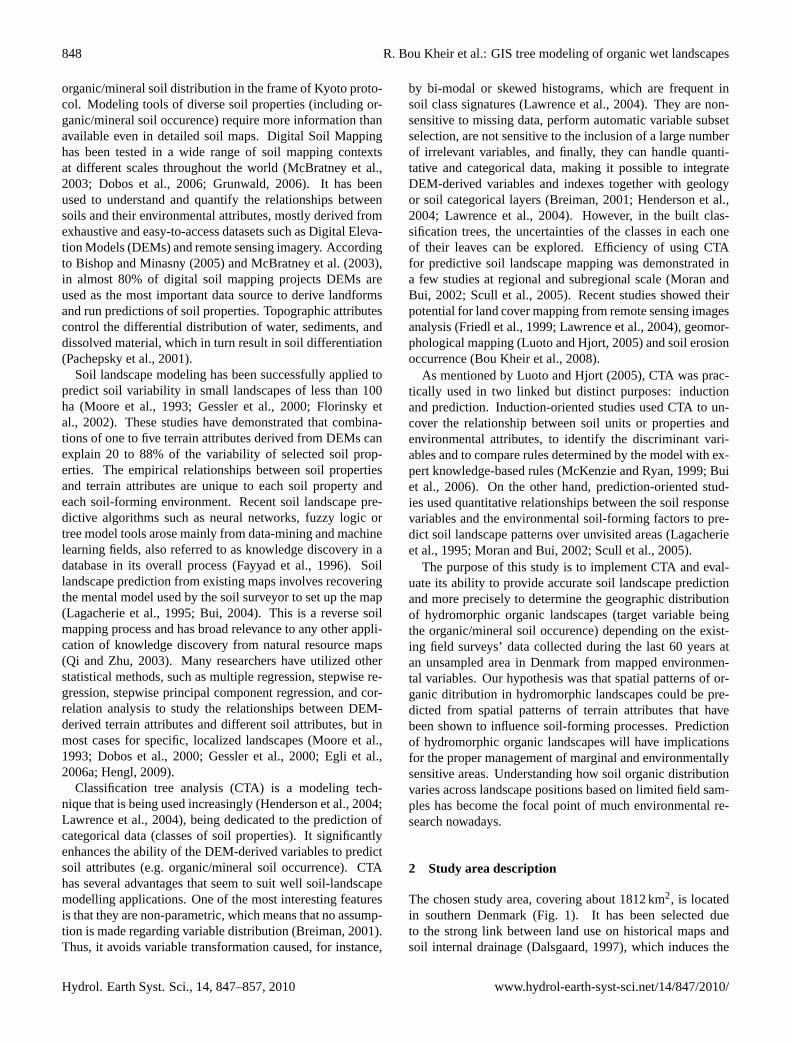
N = Number of field samples used in the modelling process; SOC = Soil Organic Carbon;

OL = Organic Landscapes; ML = Mineral Landscapes; CTI = Compound topographic

index (Steady-state wetness index); (A, B, C, D, E, F, G) = Soil type → A = coarse sandy

soil, B = Fine sandy soil, C = Clayey sand soil, D = Sandy clayey soil, E = Clayey soil, F =

Heavy clayey soil or silt soil, G = organic soil,

Fig. 2. Classification-tree model based on the combination of soil type and steady-state wetness index for predicting the spatial distributionof hydromorphic organic landscapes.

coefficient is used to measure the degree of inequality of avariable in terms of frequency distribution. It ranges be-tween 0 (perfect equality) and 1 (perfect inequality). TheGini mean difference (GMD) is defined as the mean of thedifference between each observation and every other obser-vation (Breiman, 2001) (Eq. 1):

GMD =1

N2

N∑j=1

N∑K=1

{∣∣Xj −XK∣∣} (1)

WhereX is cumulative percentage (or fractions) and theirrespective values (j andk) andN is the number of elements(observations).

Pruning the constructed trees is necessary to prevent themodels from being overfitted to the sample data, and to re-duce tree complexity. Pruning entails combining pairs of ter-minal nodes into singles nodes to determine how the mis-classification error rate changes as a function of tree size. Weused cost-complexity pruning with an independent data set (apruning data set) to produce a plot of training misclassifica-tion error rate versus tree size (Safavian and Norvig, 1991).Besides, relatively important variables can be pointed out by

counting the times the variable was used in nodes (Bui et al.,2006). However, inconsistencies within the training dataset,such as noise or outliers, can greatly affect the classifier’saccuracy (Lagacherie and Holmes, 1997).

3.5 Production of the predictive organic/inorganic land-scapes’ map

Using the preferred classification-tree model (having thehighest predictive power, and the lowest number of termi-nal nodes and predictor parameters), a predictive map of or-ganic/inorganic landscapes was obtained under a GIS envi-ronment through the application of the prediction classifica-tion tree rules (shown in Fig. 2). This map was validatedbased on field surveys.

3.6 Accuracy assessment procedure

The basis of the validation techniques was used to excludea fraction of the sample from the modeling process and tocompare the predicted value of these samples with their ref-erence value. We applied two distinct validation procedures



Table 1. The different terrain parameters (predictors) extracted from DEMs likely to impact on the organic/mineral soil distribution and theircorresponding classes.

Variable Source, description Range

Elevation Lidar Digital elevation models (DEMs) 0 to 85 mSlope From DEMs by first order finite difference 0 to 64.5◦

Aspect The direction of the steepest downslope slope 0 to 360◦

Plan curvature Curvature of contour drawn through the grid point −8.5 to 10Profile curvature Curvature of the surface in the direction of steepest descendent −9.9 to 10Tangent curvature Plan curvature multiplied by sine of slope angle −15 to 15Flow accumulation Upslope number of grid cells 1 to 59 000Flow direction Direction of the steepest drop 1 to 255Specific catchment area Upslope area per unit width of contour 32 to 8 268 160Steady-state wetness index (CTI) Modeled from DEMs; ln(As/tanβ); As is upslope catchment area,β

is slope (Moore et al., 1993)3.05 to 36.39

in order to: (i) assess to what extent the constructed clas-sification tree-models provided accurate prediction of thehydromorphic organic landscapes (internal validation), and(ii) derive the overall accuracy of the produced predictive or-ganic/inorganic landscapes’ map (external validation). Theformer uses training samples (80% of the field data or 1233sites) that were collected within the training area, whereasthe latter uses geographically distinct validation areas (20%of the field data or 308 sites). The internal validation schemeis used to test the efficiency of classification tree analysis(CTA) to predict soil landscape distribution using misclassi-fication errors. The external validation was carried out on thefull produced predictive organic/inorganic landsacpes’ map.The accuracy assessment used in the external validation issummarized in the error matrix. The matrix shows the over-all accuracy rate which is a simple ratio between the correctlyallocated number of field samples (confusion matrix diago-nal) and the overall number of classified samples.

4 Results and discussion

4.1 Derived terrain attribute maps

Ten primary and secondary topographic attribute grid mapswere obtained (Table 1). These maps displayed the surfacemorphology, zones of soil water saturation and areas likelyto have high soil organic carbon content in the study area.The steady-state topographic index (CTI) describes the dis-tribution and extent of zones of soil water saturation. Smallvalues of CTI generally depict upper catenary positions, andlarge values lower catenary positions with an overall rangetypically from around 3 to 36. The largest (i.e. high wet-ness) values are predicted in topographic hollows at higherelevations (i.e. in local areas with convergent flow lines) andimmediately above gently sloping areas near channels (i.e.footslopes) in flatted terrain.

4.2 Tree-model evaluation

Training misclassification error rates for the explanatorytrees that were developed using all variables (Model 1) ata time or the primary morphological/hydrological variablesonly (Model 2) varied from 23% to 26%, with quasi-identicalnumbers of terminal nodes (71 nodes for Model 1 and 69nodes for Model 2). The relative importance of the predictorvariables (Gini splitting method) in building those trees andsplitting the corresponding nodes is shown in Table 2.

Applying cost-complexity pruning indicated that Model 1(based on all variables) would classify correctly 67% of thetested organic/mineral soil occurence selecting just nine ter-rain variables (with their relative importance shown in paren-theses): landscape type (100%), soil type (29%), elevation(22.5%), steady-state wetness index (20%), flow accumula-tion (15%), tangent curvature (14%), aspect (11%), and slope(9%). Model 2 (based on morphological/hydrological vari-ables only) slightly reduced the explained accuracy and clas-sified 64% of the text data accurately using five variables:(1) elevation (100%), (2) slope (36%), (3) aspect (16%),(4) tangent curvature (8%), and (5) profile curvature (5%).The number of the terminal nodes was very similar for bothpruned models.

The models based on pairs of variables explained 50–68%of the variation in organic/mineral soil occurence (Table 3).The model based on soil type and steady-state topographicwetness index (CTI) (Model 3) showed the highest predic-tive power, classifying 68% of the data correctly and prunedto fourteen terminal nodes. The CTI proved to have a signif-icant contribution to the estimation of hydromorphic organiclandscapes since it is a predictor of zones of soil saturation,and organic carbon often accumulates in lowland (concave)soils for two reasons: (1) on steep slopes, dry soil conditionsprevail due to more rapid removal of water causing an impor-tant decrease in soil organic carbon, and (2) concave slopes



Table 2. Relative importance of predictor variables and misclassification error rates in Models 1 (based on all variables) and 2 (based onmorphologic/hydrologic variables only).

Predictor variables Model 1 (explanatory tree) Model 1 (Pruned tree) Model 2 (explanatory tree) Model 2 (Pruned tree)

Elevation 70% 22.5% 100% 100%Aspect 50% 11% 54% 16%Slope 37% 9% 47% 36%Profile curvature 25% 0% 23% 5%Tangent curvature 34% 14% 12% 8%Plan curvature 23% 0% 25% 0%Flow accumulation 30% 15% 4% 0%Flow direction 25% 0% 3% 0%Specific catchment area 0% 0% 0% 0%Steady-state wetness index 37% 20%Geological substrate 31% 0% Not included in building the treeSoil type 39% 29%Landscape type 100% 100%Misclassification error (%) 23% 33% 26% 36%Accuracy (%) 77% 67% 74% 64%Tree size- terminal nodes 71 9 69 10

Table 3. Accuracy explained (%) for pruned classification tree models based on pairs of variables.

Predictor variablesa a b c d e f g h i j k l m

a × 62 64 61 61 61 61 63 61 62 62 63 61b × 58 56 53 56 51 58 50 54 60 60 60c × 57 58 59 60 57 60 59 53 62 62d × 54 53 54 53 54 54 62 60 61e × 55 55 56 55 56 60 60 62f × 56 54 56 58 60 61 60g × 59 51 56 60 60 60h × 59 58 60 61 61i × 60 60 62 60j × 60 68 60k × 62 62l × 62m ×

a a = elevation, b = aspect, c = slope, d = profile curvature, e = tangent curvature, f = plan curvature, g = flow direction, h = flow direction, i= specific catchment area, j = steady-state wetness index, k = geological substrate, l = soil type, m = landscape type

can concentrate more water and sediments indicating the po-tential accumulation of a large quantity of soil organic carbon(SOC).

Without pruning, this model gave similar results to Mod-els 1 and 2 (75% of accuracy explained), but Model 3 is pre-ferred because it is easier to understand and faster to use formaking predictions. In addition, pruning the trees to their op-timal size is a required task because smaller trees may pro-vide greater predictive accuracy for unseen data than largetrees. In both Models 1 and 3, the predictor variable that wasused statistically to generate the split from the parent nodewas the soil type, indicating its potential role in predicting

the geographic location of organic landscapes. The recom-mended model (Model 3) relies on a small number of rulesand just two independent predictor variables, one of whichcan be easily and quickly constructed whenever a DEM isavailable, which is the case in most countries (Fig. 2).

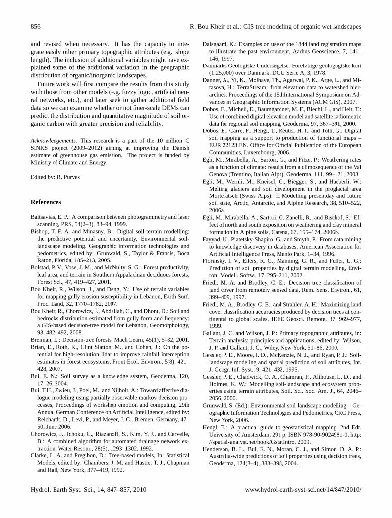
Removal of 13 variables one at a time had some effect ontraining missclassification error rates (decrease or increase)depending on the excluded variable. The three variables that,when excluded from the tree model, caused the greatest in-crease in error rate were steady state topographic wetnessindex, specific catchment area and soil type (Table 4).



27

1

2

3

4

5

Fi 6

7

8

9

10

11

12

13

14

15

16

17

18

19

20

21

22

23

24

25

26

27

28

29

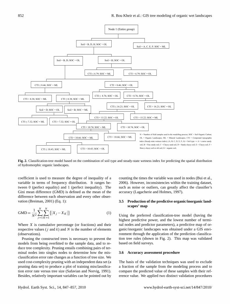
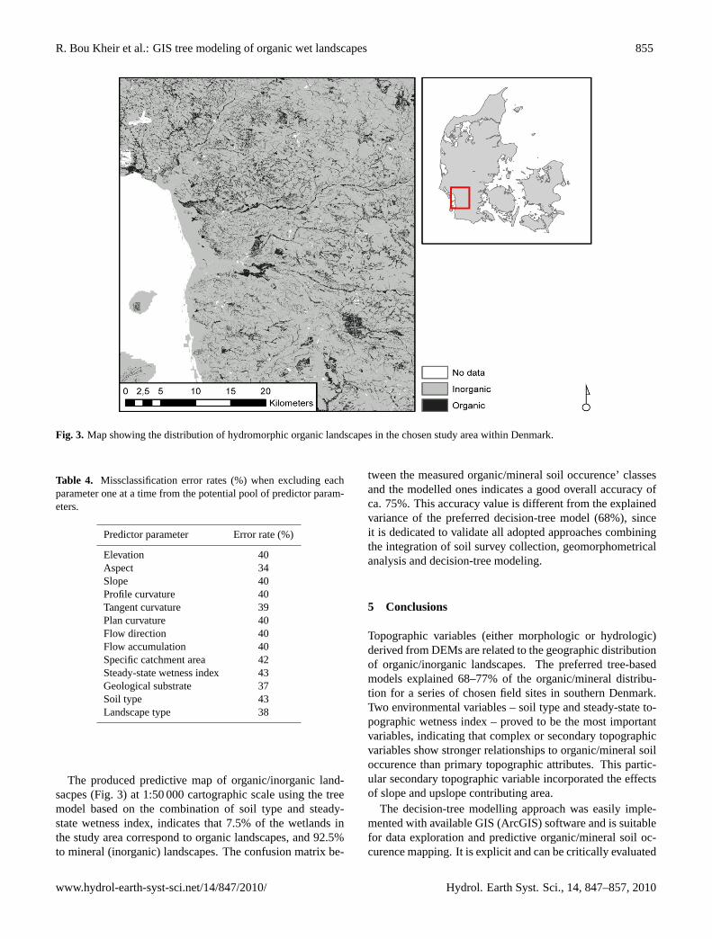
Figure 3. 30 Fig. 3. Map showing the distribution of hydromorphic organic landscapes in the chosen study area within Denmark.

Table 4. Missclassification error rates (%) when excluding eachparameter one at a time from the potential pool of predictor param-eters.

Predictor parameter Error rate (%)

Elevation 40Aspect 34Slope 40Profile curvature 40Tangent curvature 39Plan curvature 40Flow direction 40Flow accumulation 40Specific catchment area 42Steady-state wetness index 43Geological substrate 37Soil type 43Landscape type 38

The produced predictive map of organic/inorganic land-sacpes (Fig. 3) at 1:50 000 cartographic scale using the treemodel based on the combination of soil type and steady-state wetness index, indicates that 7.5% of the wetlands inthe study area correspond to organic landscapes, and 92.5%to mineral (inorganic) landscapes. The confusion matrix be-

tween the measured organic/mineral soil occurence’ classesand the modelled ones indicates a good overall accuracy ofca. 75%. This accuracy value is different from the explainedvariance of the preferred decision-tree model (68%), sinceit is dedicated to validate all adopted approaches combiningthe integration of soil survey collection, geomorphometricalanalysis and decision-tree modeling.

5 Conclusions

Topographic variables (either morphologic or hydrologic)derived from DEMs are related to the geographic distributionof organic/inorganic landscapes. The preferred tree-basedmodels explained 68–77% of the organic/mineral distribu-tion for a series of chosen field sites in southern Denmark.Two environmental variables – soil type and steady-state to-pographic wetness index – proved to be the most importantvariables, indicating that complex or secondary topographicvariables show stronger relationships to organic/mineral soiloccurence than primary topographic attributes. This partic-ular secondary topographic variable incorporated the effectsof slope and upslope contributing area.

The decision-tree modelling approach was easily imple-mented with available GIS (ArcGIS) software and is suitablefor data exploration and predictive organic/mineral soil oc-curence mapping. It is explicit and can be critically evaluated



and revised when necessary. It has the capacity to inte-grate easily other primary topographic attributes (e.g. slopelength). The inclusion of additional variables might have ex-plained some of the additional variation in the geographicdistribution of organic/inorganic landscapes.

Future work will first compare the results from this studywith those from other models (e.g. fuzzy logic, artificial neu-ral networks, etc.), and later seek to gather additional fielddata so we can examine whether or not finer-scale DEMs canpredict the distribution and quantitative magnitude of soil or-ganic carbon with greater precision and reliability.

Acknowledgements.This research is a part of the 10 millionCSINKS project (2009–2012) aiming at improving the Danishestimate of greenhouse gas emission. The project is funded byMinistry of Climate and Energy.

Edited by: R. Purves

References

Baltsavias, E. P.: A comparison between photogrammetry and laserscanning, PRS, 54(2–3), 83–94, 1999.

Bishop, T. F. A. and Minasny, B.: Digital soil-terrain modelling:the predictive potential and uncertainty, Environmental soil-landscape modeling. Geographic information technologies andpedometrics, edited by: Grunwald, S., Taylor & Francis, BocaRaton, Florida, 185–213, 2005.

Bolstad, P. V., Vose, J. M., and McNulty, S. G.: Forest productivity,leaf area, and terrain in Southern Appalachian deciduous forests,Forest Sci., 47, 419–427, 2001.

Bou Kheir, R., Wilson, J., and Deng, Y.: Use of terrain variablesfor mapping gully erosion susceptibility in Lebanon, Earth Surf.Proc. Land, 32, 1770–1782, 2007.

Bou Kheir, R., Chorowicz, J., Abdallah, C., and Dhont, D.: Soil andbedrocks distribution estimated from gully form and frequency:a GIS-based decision-tree model for Lebanon, Geomorphology,93, 482–492, 2008.

Breiman, L.: Decision-tree forests, Mach Learn, 45(1), 5–32, 2001.Brian, E., Roth, K., Clint Slatton, M., and Cohen, J.: On the po-

tential for high-resolution lidar to improve rainfall interceptionestimates in forest ecosystems, Front Ecol. Environ., 5(8), 421–428, 2007.

Bui, E. N.: Soil survey as a knowledge system, Geoderma, 120,17–26, 2004.

Bui, T.H., Zwieu, J., Poel, M., and Nijholt, A.: Toward affective dia-logue modeling using partially observable markov decision pro-cesses, Proceedings of workshop emotion and computing, 29thAnnual German Conference on Artificial Intelligence, edited by:Reichardt, D., Levi, P., and Meyer, J. C., Bremen, Germany, 47–50, June 2006.

Chorowicz, J., Ichoku, C., Riazanoff, S., Kim, Y. J., and Cervelle,B.: A combined algorithm for automated drainage network ex-traction, Water Resour., 28(5), 1293–1302, 1992.

Clarke, L. A. and Pregibon, D.: Tree-based models, In: StatisticalModels, edited by: Chambers, J. M. and Hastie, T. J., Chapmanand Hall, New York, 377–419, 1992.

Dalsgaard, K.: Examples on use of the 1844 land registration mapsto illustrate the past environment, Aarhus Geoscience, 7, 141–146, 1997.

Danmarks Geologiske Undersøgelse: Foreløbige geologogiske kort(1:25,000) over Danmark. DGU Serie A, 3, 1978.

Danner, A., Yi, K., Mølhave, Th., Agarwal, P. K., Arge, L., and Mi-tasova, H.: TerraStream: from elevation data to watershed hier-archies. Proceedings of the 15thInternational Symposium on Ad-vances in Geographic Information Systems (ACM GIS), 2007.

Dobos, E., Micheli, E., Baumgardner, M. F., Biechl, L., and Helt, T.:Use of combined digital elevation model and satellite radiometricdata for regional soil mapping, Geoderma, 97, 367–391, 2000.

Dobos, E., Carre, F., Hengl, T., Reuter, H. I., and Toth, G.: Digitalsoil mapping as a support to production of functional maps –EUR 22123 EN. Office for Official Publication of the EuropeanCommunities, Luxembourg, 2006.

Egli, M., Mirabella, A., Sartori, G., and Fitze, P.: Weathering ratesas a function of climate: results from a climosequence of the ValGenova (Trentino, Italian Alps), Geoderma, 111, 99–121, 2003.

Egli, M., Wernli, M., Kneisel, C., Biegger, S., and Haeberli, W.:Melting glaciers and soil development in the proglacial areaMorteratsch (Swiss Alps): II Modelling presentday and futuresoil state, Arctic, Antarctic, and Alpine Research, 38, 510–522,2006a.

Egli, M., Mirabella, A., Sartori, G. Zanelli, R., and Bischof, S.: Ef-fect of north and south exposition on weathering and clay mineralformation in Alpine soils, Catena, 67, 155–174, 2006b.

Fayyad, U., Piatetsky-Shapiro, G., and Smyth, P.: From data miningto knowledge discovery in databases, American Association forArtificial Intelligence Press, Menlo Park, 1–34, 1996.

Florinsky, I. V., Eilers, R. G., Manning, G. R., and Fuller, L. G.:Prediction of soil properties by digital terrain modelling, Envi-ron. Modell. Softw., 17, 295–311, 2002.

Friedl, M. A. and Brodley, C. E.: Decision tree classification ofland cover from remotely sensed data, Rem. Sens. Environ., 61,399–409, 1997.

Friedl, M. A., Brodley, C. E., and Strahler, A. H.: Maximizing landcover classification accuracies produced by decision trees at con-tinental to global scales, IEEE Geosci. Remote, 37, 969–977,1999.

Gallant, J. C. and Wilson, J. P.: Primary topographic attributes, in:Terrain analysis: principles and applications, edited by: Wilson,J. P. and Gallant, J. C., Wiley, New York, 51–86, 2000.

Gessler, P. E., Moore, I. D., McKenzie, N. J., and Ryan, P. J.: Soil-landscape modeling and spatial prediction of soil attributes, Int.J. Geogr. Inf. Syst., 9, 421–432, 1995.

Gessler, P. E., Chadwick, O. A., Chamran, F., Althouse, L. D., andHolmes, K. W.: Modelling soil-landscape and ecosystem prop-erties using terrain attributes, Soil. Sci. Soc. Am. J., 64, 2046–2056, 2000.

Grunwald, S. (Ed.): Environmental soil-landscape modelling – Ge-ographic Information Technologies and Pedometrics, CRC Press,New York, 2006.

Hengl, T.: A practical guide to geostatistical mapping, 2nd Edt.University of Amsterdam, 291 p, ISBN 978-90-9024981-0,http://spatial-analyst.net/book/GstatIntro, 2009.

Henderson, B. L., Bui, E. N., Moran, C. J., and Simon, D. A. P.:Australia-wide predictions of soil properties using decision trees,Geoderma, 124(3–4), 383–398, 2004.


http://spatial-analyst.net/book/GstatIntro

http://spatial-analyst.net/book/GstatIntro


IPCC: Land-use, land-use change, and forestry, in: Land-use, land-use change, and forestry, edited by: Watson, R. T., Noble, I. R.,Bolin, B., Ravindranath, N. H., Verardo, D. J., and Dokken, D.J., A special report to the Intergovernmental Panel on ClimateChange (IPCC), Cambridge University Press, Cambridge, UK,1–51, 2000.

Lagacherie, P. and Holmes, S.: Addressing geographical data errorsin a classification tree for soil unit prediction, Int. J. Geogr. Inf.Sci., 11, 183–198, 1997.

Lagacherie, P., Legros, J. P., and Burrough, P. A.: A soil survey pro-cedure using the knowledge of soil pattern established on a pre-viously mapped reference area, Geoderma, 65, 283–301, 1995.

Lawrence, R., Bunn, A., Powell, S., and Zambon, M.: Classificationof remotely sensed imagery using stochastic gradient boosting asa refinement of classification tree analysis, Rem. Sens. Environ.,90, 331–336, 2004.

Lees, B. G. and Ritman, K.: Decision-tree and rule-induction ap-proach to integration of remotely sensed and GIS data in map-ping vegetation in distributed hilly environments, J. Environ.Manage., 15, 823–831, 1991.

Loh, W. Y. and Shih, Y. S.: Split selection methods for classificationtrees, Stat Sinica, 7, 815–840, 1997.

Liu, X.: Airborne LiDAR for DEM generation: some critical issues,Progress Prog. Phys. Geog., 32(1), 31–49, 2008.

Luoto, M. and Hjort, J.: Evaluation of current statistical approachesfor predictive geomorphological mapping, Geomorphology, 67,299–315, 2005.

Madsen, H. B., Nørr, A. H., and Holst, K. A.: The Danish SoilClasification. Atlas over Denmark I,3. The Royal Danish Geo-graphical Society, Copenhagen, 1992.

McBratney, A. B., Mendonca, M. L., and Minasny, B.: On digitalsoil mapping, Geoderma, 117, 3–52, 2003.

McKenzie, N. J. and Ryan, P. J.: Spatial prediction of soil propertiesusing environmental correlation, Geoderma, 89, 67–94, 1999.

Moore, I. D., Gessler, P. E., Nielsen, G. A., and Peterson, G. A.: Soilattribute prediction using terrain analysis, Soil Sci. Soc. Am. J.,57, 443–452, 1993.

Moran, C. J. and Bui, E. N.: Spatial data mining for enhanced soilmap modeling, Int. J. Geogr. Inf. Sci., 16, 533–549, 2002.

Pachepsky, Y. A., Timlin, D. J., and Rawls, W. J.: Soil water reten-tion as related to topographic variables, Soil Sci. Soc. Am. J., 65,1787–1795, 2001.

Qi, F. and Zhu, A. X.: Knowledge discovery from soil maps usinginductive learning, Int. J. Geogr. Inf. Syst., 17(8), 771–795, 2003.

Safavian, S. J. and Norvig, P.: A survey of tree classifier methodol-ogy, IEEE T. Syst. Man. Ct. A, 21, 660–674, 1991.

Scull, P., Franklin, J., and Chadwick, O. A.: The application ofclassification tree analysis to soil type prediction in a desert land-scape, Ecol. Model., 181, 1–15, 2005.

Schmitt, N. P., Rehm, W. F., Pistner, T., Zeller, P., Diehl, H., andNave, P.: The AWIATOR airborne LIDAR turbulence sensor,Aerospace Sci. Technol., 11(7–8), 546–552, 2007.

Tarboton, D. G., Bras, R. L., and Rodriguez-Iturbe, I.: On the ex-traction of channel networks from digital elevation data, Hydrol.Processes, 5, 81–100, 1991.

Thompson, J. A. and Kolka, R. K.: Soil carbon storage estimation ina forested watershed using quantitative soil-landscape modelling,Soil Sci. Soc. Am. J., 69, 1086–1093, 2005.

Wilson, J. P. and Gallant, J. C.: Secondary topographic attributes,in: Terrain analysis: principles and applications, edited by: Wil-son, J. P. and Gallant, J. C., Wiley: New York, 87–132, 2000.


Documents

The application of GIS based decision-tree models for ... · R. Bou Kheir et al.: GIS tree modeling of organic wet landscapes 849 25 1 Fig. 1. Soil map of the study area within Denmark